Resource-Aware Query Scheduling in Database Management Systems by Natalie Gruska A thesis submitted to the School of Computing in conformity with the requirements for the degree of Master of Science Queen’s University Kingston, Ontario, Canada June 2011 Copyright c Natalie Gruska, 2011
Database Management Systems (DBMSs) are the primary tools used for storing and
accessing data and they are the backbone of many applications. A single DBMS
can receive many concurrent requests which it must handle. The type of requests a
database receives, also called the workload, can vary. Consider an e-commerce site,
as customers are buying products, updates are made to the inventory data to keep
numbers current. At the same time, business managers want to query inventory data
to determine facts such as which products are best-sellers. These two situations ex-
emplify the two fundamental database workload types: online transaction processing
(OLTP) and online analytical processing (OLAP)—also referred to as Business In-
telligence (BI). An OLTP workload is characterized by many short transactions and
numerous updates. For instance, an update of an inventory number is quick and
needs to only touch a very small amount of data. OLAP workloads on the other
hand, usually consist of longer, more resource intensive queries. They tend to re-
quire reading large amounts of data and more complex processing (sorting, finding
the maximum, calculating totals). Certainly, these workloads are not always distinct
and it is possible to have both OLTP and OLAP type requests acting on a single
database. The number and mix of requests that a DBMS has to handle varies over
1
CHAPTER 1. INTRODUCTION 2
time. There can be regular fluctuations in the workload such as an increase in sales
during lunch time on weekdays, or seasonal changes such as a large increase in sales
before Christmas.
Since a database has limited physical resources such as CPU and memory, there
is a limit to the number of requests it can process concurrently. Too many concur-
rent requests lead to resource contention, which can cause the performance of the
database to drop drastically. The number of requests that a database is able to
handle depends on a variety of factors such as the system hardware, the system con-
figuration and the workload. In addition to system overload, which leads to resource
contention, system underutilization can also be a problem. If the concurrency level of
a database is limited too much, resources are left idle, which causes the database to
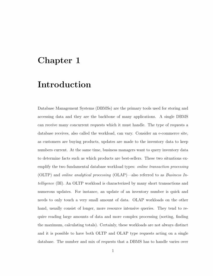
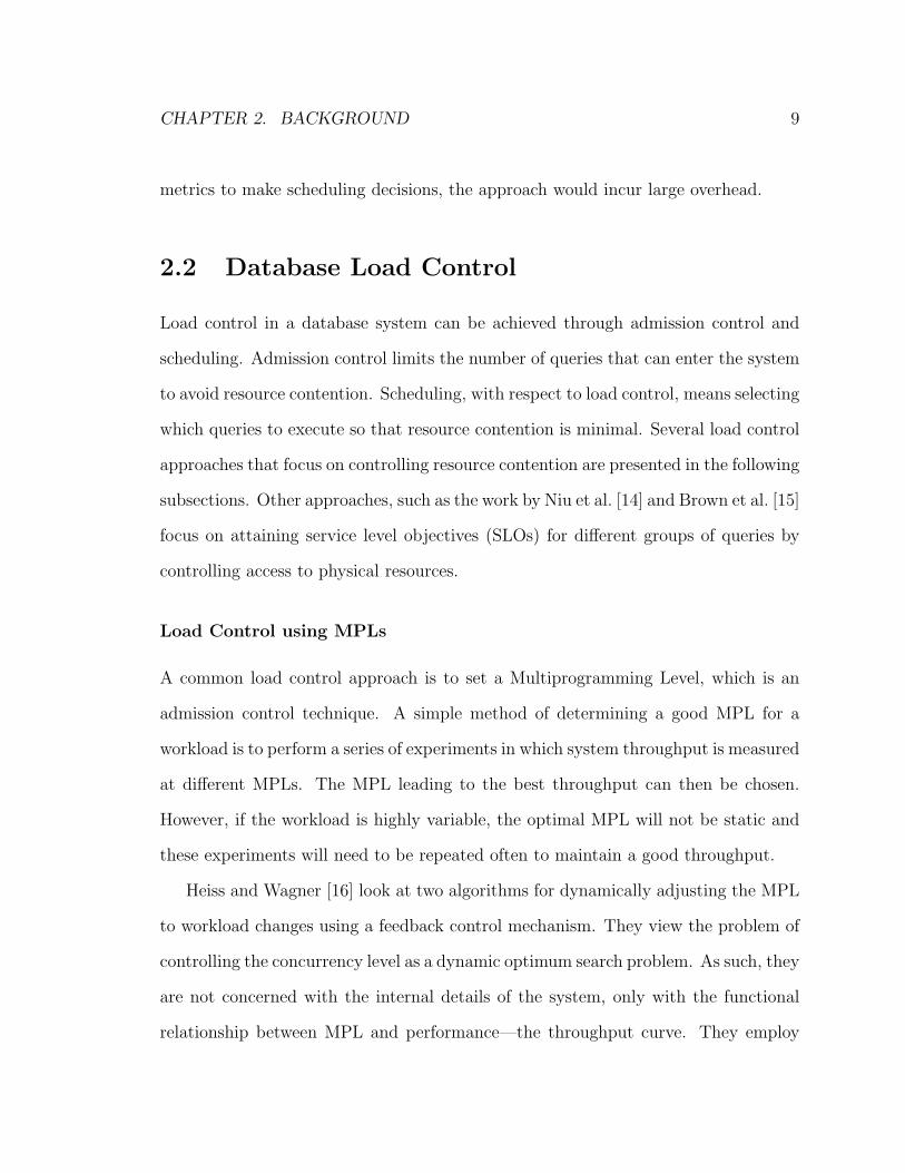
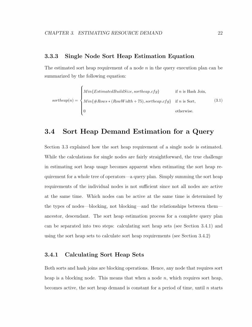
perform below its potential. This relationship can be seen by examining a throughput
curve. A throughput curve shows the relationship between concurrency level and the
database’s throughput under a certain workload, on a specific system. The number
of concurrently running requests in a database is also referred to as the multipro-
gramming level (MPL). Typically a throughput curve has a fairly parabolic shape;
a sample curve is shown in Figure 1.1. Up to a certain threshold, an increase in
MPL causes the throughput to rise (the underloaded phase), then there is an optimal
range in which the curve is relatively flat, but once the MPL increases more than the
optimal range, the system becomes overloaded and throughput drops sharply. The
goal of a load control system should be to maintain throughput in the optimal range.
Controlling load on a DBMS is not an easy task since not all requests are equal
in the amount of resources they require. Setting a static limit for the total number of
requests that are allowed to execute may work well if requests are relatively equal in
CHAPTER 1. INTRODUCTION 3
Figure 1.1: Throughput curves showing the relationship between MPL and throughput fordifferent workload sizes. The throughput curve for the medium workload is divided into threesystem states: underload, optimal, and overload. [1]
their resource requirements, but will lead to suboptimal performance if the requests
are extremely varied, for instance, a mix of OLTP and OLAP queries. Beyond the
amount of resource demand, queries can also differ in the type of resources they re-
quire. For instance, I/O intensive queries primarily read data, CPU intensive queries
require a lot of calculations, memory intensive queries may store many partial re-
sults. If the mix of queries being executed is not balanced, then one resource may be
overloaded while others are idle. A load control system should be able to effectively
handle all of these factors and adapt to current conditions.
Current trends such as server consolidation [2, 3] and an increased reliance on
business analytics [4, 5] are increasing the complexity of the workloads which DBMSs
are required to handle. Server consolidation is an approach to save costs by combining
workloads traditionally run on different servers onto a single server. This means that
analytics workloads are no longer separated from day-to-day operational workloads.
Hence, the mix of requests that a single DBMS is expected to process at any point
in time is highly variable; from long resource-intensive queries to quick updates.
CHAPTER 1. INTRODUCTION 4
Businesses are also increasingly relying on business intelligence to make decisions.
Managers want up-to-date data instantly, and are not willing to wait hours before
being able to run a BI query. Therefore, the DBMS has to be able to manage these
complex queries at any time and be able to perform optimally no matter what type,
or how many queries are presented.
1.1 Research Statement
The objective of our research is to investigate the feasibility of a database load control
system based on regulating individual resource consumption in a predictive manner.
This means treating system resources, such as CPU, memory (bufferpool, sort heap,
etc.), and I/O, separately. The amount of each of these resources that a query re-
quires is predicted when the query is submitted to the DBMS. These predictions are
then used to determine whether the query is a good fit to execute based on current
conditions. If the query requires resources that are available, then it is allowed to run.
However, if the query requires resources which are already at capacity, it may have to
wait for resources to become available before being allowed to execute. To reduce the
complexity of this problem, the scope of this work is limited to one specific resource;
namely, the sort heap. The sort heap is a section of memory that is reserved for
performing specific operations such as sorting data. This resource is primarily used
by queries that require complex data processing; namely, OLAP workloads.
Our work makes two main contributions. Firstly, we present a method of es-
timating the sort heap demand of a query based on the query execution plan. The
second contribution is a prototype load control system based on these estimations. We
compare the effectiveness of three different scheduling methods using the prototype
system.
CHAPTER 1. INTRODUCTION 5
1.2 Thesis Organization
The remainder of this thesis is organized as follows. Chapter 2 covers background
and related work. Chapter 3 presents our method for estimating resource demand
and an evaluation of this method. Chapter 4 describes our prototype load control
system and three proposed query scheduling methods. It also includes an evaluation
of this system. Finally, Chapter 5 contains concluding remarks and describes future
work.
Chapter 2
Background
There are two general areas of research that relate to our work; query metric esti-
mation and load control methods. Work on estimating query metrics is discussed in
Section 2.1. Different load control methods are presented in Section 2.2.
2.1 Query Metric Estimation
Estimating query metrics such as the amount of memory a query will require or
the time it will take to execute is a challenging problem. Much of the work in this
area has focused on estimating query runtime and progress [6, 7, 8, 9]. The body of
work addressing physical resource requirement estimation is rather limited. Database
Query Optimizers use a cost metric to represent the resource requirements of a specific
query plan. Sacco and Schkolnick [10] use an analytical approach to characterize
a query’s buffer pool requirements. Ganapathi et al. [11] use a machine learning
approach to predict a variety of query metrics. These approaches are discussed in
more detail in the following subsections.
6
CHAPTER 2. BACKGROUND 7
Query Optimizers
Query Optimizers calculate the cost of different query plans in order to compare the
plans and choose the most efficient one. The factors considered when calculating this
cost differs among DBMSs. DB2 [12] measures cost in timerons. Timerons represent
an estimate of the CPU cost (number of instructions) and the I/O cost (number of
seeks and page transfers) of a plan. This is a rough estimate of the required resources
and a timeron does not equate to any actual elapsed time. PostgreSQL [13] measures
cost by estimating how long it will take to run a statement in terms of units of disk
page fetches. Query optimizer cost estimations are useful for their purpose; namely,
selecting a good execution plan. However, they are not suitable for scheduling to
control resource consumption since they are usually an aggregate of various resources
and do not necessarily correlate to the actual resources used.
Buffer Requirements
Sacco and Schkolnick [10] characterize the buffer requirements of queries in an analyt-
ical fashion. The number of page faults that occur when processing a query depends
on the size of the buffer pool. They refer to this relationship between buffer size
and page faults as a query’s fault curve. The fault curve consists of a number of
stable intervals (for which the number of page faults is constant), separated by dis-
continuities. The exact shape of a fault curve depends on the page reuse pattern.
The authors present several different patterns: simple reuse, loop reuse, unclustered
reuse, and index reuse. A hot point is defined as the value of the fault function at the
start of a stable interval. A query’s optimal buffer requirement is defined to be the
largest hot point on its fault curve that does not exceed system buffer space. Like
CHAPTER 2. BACKGROUND 8
our approach, Sacco and Schkolnick determine the amount of a physical resource that
a query will require. However, the physical resource addressed in their work differs
from the physical resource addressed in our work. Furthermore, the optimal buffer
requirement of a query needs to be determined analytically while our approach can
automatically calculate required sort heap space using the query execution plan.
Predicting Performance Metrics
Ganapathi et al. [11] present a query metric prediction tool based on machine learning.
The tool is able to estimate a variety of metrics such as the number of records used,
disk I/O, and execution time. Like our estimation approach, Ganapathi et al. extract
information from the query execution plan to make their predictions. Specifically,
they extract feature vectors which contain an instance count and cardinality sum for
each operator in the plan. Kernel canonical correlation analysis (KCCA) is then used
to create predictive models and make predictions. The authors’ experiments showed
that if a large set of training data is available, their prediction method works very
well. However, if only a small set of training data is available, or the training and
test queries are executed against different databases, the accuracy of the predictions
greatly suffers. Although a variety of metrics are estimated, physical memory usage
is not included. The purpose of the metrics predicted by Ganapathi et al. is more
to assist in identifying long-running or abnormal queries, rather than for scheduling
or load control purposes. The authors state that the prediction for a single query
can be done in under a second, making this machine learning approach practical for
queries that take minutes or hours to run, but not for shorter queries. If one were to
calculate predictions for every incoming query, as would be required when using the
CHAPTER 2. BACKGROUND 9
metrics to make scheduling decisions, the approach would incur large overhead.
2.2 Database Load Control
Load control in a database system can be achieved through admission control and
scheduling. Admission control limits the number of queries that can enter the system
to avoid resource contention. Scheduling, with respect to load control, means selecting
which queries to execute so that resource contention is minimal. Several load control
approaches that focus on controlling resource contention are presented in the following
subsections. Other approaches, such as the work by Niu et al. [14] and Brown et al. [15]
focus on attaining service level objectives (SLOs) for different groups of queries by
controlling access to physical resources.
Load Control using MPLs
A common load control approach is to set a Multiprogramming Level, which is an
admission control technique. A simple method of determining a good MPL for a
workload is to perform a series of experiments in which system throughput is measured
at different MPLs. The MPL leading to the best throughput can then be chosen.
However, if the workload is highly variable, the optimal MPL will not be static and
these experiments will need to be repeated often to maintain a good throughput.
Heiss and Wagner [16] look at two algorithms for dynamically adjusting the MPL
to workload changes using a feedback control mechanism. They view the problem of
controlling the concurrency level as a dynamic optimum search problem. As such, they
are not concerned with the internal details of the system, only with the functional
relationship between MPL and performance—the throughput curve. They employ
CHAPTER 2. BACKGROUND 10
two optimum search algorithms to automatically tune the MPL; incremental steps
and parabola approximation. Through the use of a simulation model, Heiss and
Wagner show that both algorithms are efficient at finding the optimal MPL when the
workload is static and are also efficient at adjusting the MPL to gradual workload
changes. Parabola approximation is superior at adjusting the MPL when the workload
changes quickly and drastically since it is able to modify the MPL in larger increments.
In 2010, Abouzour et al. [17] revisited the algorithms presented by Wager and
Heiss with slight optimizations. They also propose a hybrid of the two algorithms; hill
climbing for several intervals and then parabola approximation for one interval. This
combination allows the system to make quick adjustments without large oscillations.
While generally coming to the same conclusions as Heiss and Wagner, Abouzour et al.
also note that this form of automatic MPL tuning is not well suited for all workload
types. For instance, workloads that have a pattern of bursty requests are not handled
well. The approach is best for workloads with a continuous stream of requests.
Schroeder et al. [18] look at the challenge of setting the MPL from a scheduling
angle. Usually when scheduling queries externally, all queries that are not immedi-
ately executed are put into a queue. The larger this queue, the more choice when
selecting the next query to execute and the more likely that a suitable query will be in
the queue. Hence, Schroeder et. al’s work focuses on how low the MPL can be set so
that throughput will not suffer while having a large amount of control over schedul-
ing. Queueing theoretic models and a feedback control loop are used to predict the
relationship between throughput, MPL and response time and to optimize the MPL.
While Schroeder et al. evaluate this approach by examining its effect on workloads
with query priorities in which high priority queries should be chosen to run first, it is
CHAPTER 2. BACKGROUND 11
also relevant in terms of scheduling for resource control. If the queue is larger, then a
query with resource requirements suitable to the currently available resources is more
likely to be found.
Alternative Load Control Approaches
Although the number of concurrently running queries has a major impact on per-
formance, setting an MPL may not always be the correct solution to keep a DBMS
running efficiently. When limiting the number of queries in a database system through
a multiprogramming level, all queries are treated as equal. If the MPL is five, then five
queries are allowed to run concurrently no matter how computationally or I/O expen-
sive they are. If queries in the workload vary greatly in their resource requirements,
then treating them equally can lead to suboptimal system performance. In these
cases, properties of individual queries should be taken into account when considering
how many, and which requests to run concurrently.
Mehta et al. [1] focus on scheduling batch workloads. For batch workloads, the
important measure is overall response time, not the response time of the individual
queries or throughput, since all the queries need to be processed before the work
can be considered completed. The general approach of their workload management
system can be summarized in four steps:
1. Determine a variable whose value is suitable for BI workload management de-
cisions
2. Admit queries based on some value of the manipulated variable
3. Schedule queries so that system behaves optimally
CHAPTER 2. BACKGROUND 12
4. Make system stable over wide range of the manipulated variable (make the
system tolerant to prediction errors)
Traditionally MPL has been used as the manipulated variable, but as mentioned, MPL
is very vulnerable to workload changes. Mehta et al. suggest the use of a different
variable: memory. They note that any resource that causes a bottleneck may be a
good choice as manipulated variable. These four steps are similar to those in our
approach, but instead of general memory being the manipulated variable, we focus
on the sort heap. Mehta et al.’s workload management divides the batch of queries
to be processed into sub-batches, so that the memory requirement of the queries in
each sub-batch adds up to available memory. Our approach is not limited to batch
workloads. Mehta et al. do not discuss how memory requirements of individual
queries or workloads are determined in their approach. They refer to the work by
Sacco and Schkolnick [10], however they do not mention if this is the technique they
implement.
Ahmad et al. [19] propose an interaction-based scheduler. Concurrent queries can
negatively affect each other but they can also positively affect each other, meaning
their concurrent run-time is faster than the time it takes to run both queries individu-
ally. To optimize performance, one needs to consider query mixes. There are numer-
ous possible causes of query interactions including resource-related, data-related and
configuration-related dependencies. Furthermore system settings and hardware have
an effect. Ahmad et al. propose an experiment-driven approach to solve this problem.
Their approach is tailored towards BI workloads with a set number of query types.
The approach involves running a small set of carefully chosen query mixes and also
running each query type in isolation. The results of these experiments are then used
CHAPTER 2. BACKGROUND 13
to calculate how the completion time of a specific query is affected by the mix. This
experiment-driven approach has two main advantages. Firstly, it is independent of
the root cause of the interaction because the interaction is captured in data collected
from the experiments. Secondly, it supports incremental updates as query workloads
evolve or new query types are added. The authors developed a query scheduler called
QShuffler. It is assumed that the system has a static multiprogramming level which
limits the number of queries that are executed concurrently. A linear program is used
to consider different query mixes and find the schedule with the minimum completion
time.
Chapter 3
Estimating Resource Demand
For a load control system based on regulating individual resource usage to be success-
ful, it has to be able to estimate the amount of resources a query requires. There are
many resources such as CPU, buffer pools, sort heap, and disk I/O, which should be
taken into account to achieve a complete picture of a query’s resource requirements.
We focus here on a single resource, sort heap, as a proof-of-concept. The sort heap
is a section of memory that is reserved for specific operations such as sorting and
certain types of joins.
When a query is submitted to a database system, the system creates a query
execution plan which consists of a detailed breakdown of how the query will be pro-
cessed. A query execution plan consists of operators linked together in a tree-like
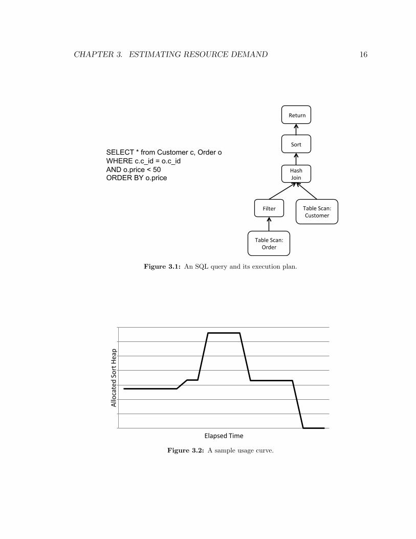
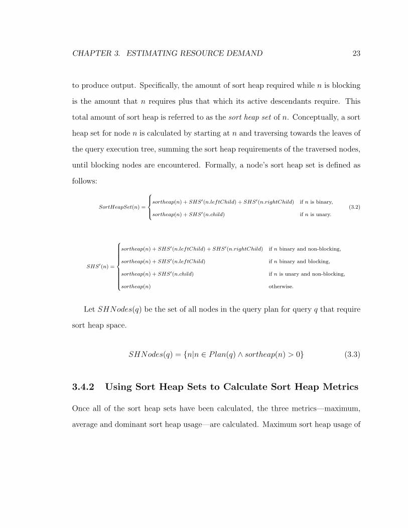
structure. Operators are operations such as joins, sorts, and filters. Figure 3.1 shows
an example of an SQL query and a high-level representation of its execution plan.
The plan outlines the following processing steps: the Order table is filtered to remove
tuples whose price value is greater than 50, the remaining tuples are joined with the
tuples in the Customer table and the result of the join is sorted so that the output
tuples are ordered by price. Some of the operations in this query plan, the sort and
the hash join, require the use of sort heap memory to perform their processing tasks.
14
CHAPTER 3. ESTIMATING RESOURCE DEMAND 15
Appendix A contains further information on DB2 query execution plans.
The sort heap was chosen as the focus resource for several reasons. Firstly, it is
a measurable and accessible quantity; it is possible to measure the current amount
of sort heap being used by the system. Since prediction and scheduling are happen-
ing externally, it is important that the chosen resource is accessible from outside the
database system. Sort heap is a quantifiable resource; available sort heap can be
expressed in terms of free bytes and the sort heap requirement of a query can also
be expressed in bytes. Such a quantifiable amount is comparable and additive. Fur-
thermore, sort heap space is bounded; at any point in time there is a limited amount
of sort heap space available. Choosing a bounded resource simplifies the scheduling
aspect of this workload management approach since it provides a fixed resource limit
when considering which queries to run. Sort heap usage also affects DBMS perfor-
mance. If queries require more sort heap space than is available, this will lead to an
increase in I/O and processing times. The performance aspects of the sort heap are
discussed in more detail in Chapter 4.
Estimating sort heap usage is not without challenges, which are discussed in Sec-
tion 3.1. Section 3.2 outlines the chosen estimation method, and Sections 3.3 and
3.4 present the estimation steps in detail. The effectiveness of the sort heap demand
estimations is shown through an evaluation in Section 3.6.
3.1 Challenges of Estimating Sort Heap Demand
A query execution plan describes the general sequence of steps that are taken to
produce the query result, with each step being an operator. However, more than one
operator can be active at the same time. For instance, consider the plan in Figure
CHAPTER 3. ESTIMATING RESOURCE DEMAND 16
SELECT * from Customer c, Order o WHERE c.c_id = o.c_id AND o.price < 50 ORDER BY o.price
Table Scan: Customer
Table Scan: Order
Sort
Hash Join
Filter
Return
Figure 3.1: An SQL query and its execution plan.
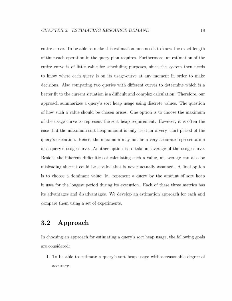
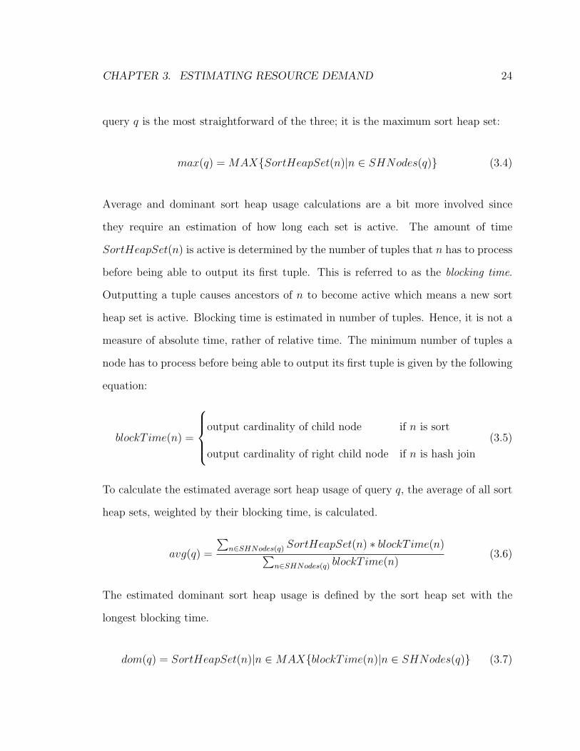
Allocated Sort Heap
Elapsed Time
Figure 3.2: A sample usage curve.
CHAPTER 3. ESTIMATING RESOURCE DEMAND 17
3.1, in which a table scan operator is followed by a filter operator. The DBMS does
not complete the table scan, and then go on to the filter, it performs both operations
at the same time. A tuple that is read from the table goes directly to the filtering
step. This is referred to as pipelining. Pipelining is not always possible due to the
existence of blocking operators. These are operators which need to receive at least
one complete input before being able to produce any output. For instance, a sort
operator is a blocking operator. Since the sort operator outputs its tuples in sorted
order, it has to wait until it has received all its input tuples before it can decide which
one is smallest—or largest. Binary blocking operators, ie. those that take two inputs,
need to receive the complete input from the right child before the they can produce
any output.
Each operation involved in calculating the result of a query (select, project, join,
sort, etc.) varies in the amount of time and sort heap it requires. In addition, a sort
operation on a small table will require less sort heap than a sort operation on a larger
table—assuming a constant tuple size. Because different sets of operators are active
at different times, a query’s sort heap requirement varies throughout its execution.
The relationship between elapsed time and sort heap usage during the execution of a
query will be referred to as the query’s usage curve. Figure 3.2 shows a usage curve
depicting the sort heap usage of the query plan in Figure 3.1. The sort heap usage
is at a constant level while just the hash join operator is active, it then jumps to a
higher level as both the sort and hash join operators become active and then returns
to a lower level when the hash join is finished and just the sort operator is active.
The fluctuations of a query’s usage curve pose a challenge when estimating the
query’s sort heap requirement. It is difficult to accurately estimate the shape of the
CHAPTER 3. ESTIMATING RESOURCE DEMAND 18
entire curve. To be able to make this estimation, one needs to know the exact length
of time each operation in the query plan requires. Furthermore, an estimation of the
entire curve is of little value for scheduling purposes, since the system then needs
to know where each query is on its usage-curve at any moment in order to make
decisions. Also comparing two queries with different curves to determine which is a
better fit to the current situation is a difficult and complex calculation. Therefore, our
approach summarizes a query’s sort heap usage using discrete values. The question
of how such a value should be chosen arises. One option is to choose the maximum
of the usage curve to represent the sort heap requirement. However, it is often the
case that the maximum sort heap amount is only used for a very short period of the
query’s execution. Hence, the maximum may not be a very accurate representation
of a query’s usage curve. Another option is to take an average of the usage curve.
Besides the inherent difficulties of calculating such a value, an average can also be
misleading since it could be a value that is never actually assumed. A final option
is to choose a dominant value; ie., represent a query by the amount of sort heap
it uses for the longest period during its execution. Each of these three metrics has
its advantages and disadvantages. We develop an estimation approach for each and
compare them using a set of experiments.
3.2 Approach
In choosing an approach for estimating a query’s sort heap usage, the following goals
are considered:
1. To be able to estimate a query’s sort heap usage with a reasonable degree of
accuracy.
CHAPTER 3. ESTIMATING RESOURCE DEMAND 19
2. To make estimations without prior knowledge of queries or query types.
3. To make estimations independent of system configuration and hardware.
4. To make estimations in such a way that they could easily be integrated into
existing query optimizers.
An automated analytical approach is able to achieve these goals. Since the rela-
tionship between the query execution plan and sort heap usage is known, it can be
analytically defined. The chosen approach limits itself solely to the information that
is available in the query execution plan and does not require any training. Hence,
no prior knowledge of the queries is required and estimations can be made for never
before encountered queries. Since query optimizers already calculate cost estimates
based on the query execution plan, an additional sort heap cost estimate does not
incur much overhead and can be easily integrated into existing query optimizers.
The chosen approach considers the operators, cardinalities and relationship between
operators in the query execution plan to calculate a query’s sort heap usage.
The estimation approach consists of two steps; estimating the sort heap require-
ment of single operators (see Section 3.3), and then using these estimates to calculate
an estimate for the complete query plan (see Section 3.4).
3.3 Sort Heap Demand Estimation for a Single
Operator
Only two DB2 operators require sort heap space; sort and hash join. The query
execution plan, attained through db2expln (see Appendix A), provides information
CHAPTER 3. ESTIMATING RESOURCE DEMAND 20
on the amount of sort heap space each of these operators requires. The next two
sections detail the available information and how it is used to estimate sort heap
usage for a single operation.
3.3.1 Sort Operator
The following is an excerpt from a query plan, showing the information that is relevant
to sort heap usage for a sort operation:
Sortheap Allocation Parameters:
#Rows = 121929
Row Width = 44
#Rows refers to the number of rows to be sorted and Row Width is the approximate
width of each row in bytes. A rough estimate of the required sort heap space is given
by multiplying these two numbers together. However, an overhead of at least 32 bytes
per row is added to this required space.1 Experimentally, it was determined that 75
bytes per row is a good approximation of the additional overhead. Another factor to
consider when estimating required sort heap space is a configuration parameter called
sortheap cfg (see Section 3.6.1). This parameter limits the maximum amount of sort
heap space that can be assigned to a single sort or hash join. Hence, the final sort
heap estimate for a sort is calculated using the following formula:
Min{#Rows*(Row Width + 75), sortheap cfg}1The exact value of the overhead is not observable from outside the system. The amount of
overhead varies with the specific type of sort that is used and other factors. This information wasacquired through a personal communication with a DB2 developer.
CHAPTER 3. ESTIMATING RESOURCE DEMAND 21
3.3.2 Hash Join Operator
The following is an excerpt from a query plan, showing the information that is relevant
to sort heap usage for a hash join operation:
Hash Join
Estimated Build Size : 24000
Estimated Probe Size : 98500000
Bit Filter Size: 16500
Estimated Build Size refers to the size, in bytes, of the relation that is to be
stored in a hash table and Estimated Probe Size refers to the size, in bytes, of
the relation that is used to probe the hash table. Of these two sizes, only the build
size is relevant to the estimation of sort heap demand since only the hash table is
stored in sort heap memory. Bit Filter Size is only indicated if a bit filter is
going to be used. A bit filter is an array of bits which can be used to improve hash
join performance. It is used to efficiently determine whether a tuple from the probe
relation will match with one from the build relation. The bit filter is also stored in
sort heap memory and hence adds to the required sort heap. As with sorts, hash
joins are restricted by the sortheap cfg parameter. The following formula is used to
calculate the sort heap requirement of a single hash join.
Min{Estimated Build Size + Bit Filter Size, sortheap cfg}
CHAPTER 3. ESTIMATING RESOURCE DEMAND 22
3.3.3 Single Node Sort Heap Estimation Equation
The estimated sort heap requirement of a node n in the query execution plan can be
summarized by the following equation:
sortheap(n) =
Min{EstimatedBuildSize, sortheap cfg} if n is Hash Join,
Min{#Rows ∗ (RowWidth + 75), sortheap cfg} if n is Sort,
0 otherwise.
(3.1)
3.4 Sort Heap Demand Estimation for a Query
Section 3.3 explained how the sort heap requirement of a single node is estimated.
While the calculations for single nodes are fairly straightforward, the true challenge
in estimating sort heap usage becomes apparent when estimating the sort heap re-
quirement for a whole tree of operators—a query plan. Simply summing the sort heap
requirements of the individual nodes is not sufficient since not all nodes are active
at the same time. Which nodes can be active at the same time is determined by
the types of nodes—blocking, not blocking—and the relationships between them—
ancestor, descendant. The sort heap estimation process for a complete query plan
can be separated into two steps: calculating sort heap sets (see Section 3.4.1) and
using the sort heap sets to calculate sort heap requirements (see Section 3.4.2)
3.4.1 Calculating Sort Heap Sets
Both sorts and hash joins are blocking operations. Hence, any node that requires sort
heap is a blocking node. This means that when a node n, which requires sort heap,
becomes active, the sort heap demand is constant for a period of time, until n starts
CHAPTER 3. ESTIMATING RESOURCE DEMAND 23
to produce output. Specifically, the amount of sort heap required while n is blocking
is the amount that n requires plus that which its active descendants require. This
total amount of sort heap is referred to as the sort heap set of n. Conceptually, a sort
heap set for node n is calculated by starting at n and traversing towards the leaves of
the query execution tree, summing the sort heap requirements of the traversed nodes,
until blocking nodes are encountered. Formally, a node’s sort heap set is defined as
follows:
SortHeapSet(n) =
8>><>>:sortheap(n) + SHS′(n.leftChild) + SHS′(n.rightChild) if n is binary,
sortheap(n) + SHS′(n.child) if n is unary.
(3.2)
SHS′(n) =
8>>>>>>>>><>>>>>>>>>:
sortheap(n) + SHS′(n.leftChild) + SHS′(n.rightChild) if n binary and non-blocking,
sortheap(n) + SHS′(n.leftChild) if n binary and blocking,
sortheap(n) + SHS′(n.child) if n is unary and non-blocking,
sortheap(n) otherwise.
Let SHNodes(q) be the set of all nodes in the query plan for query q that require
There are several limitations to the chosen demand estimation method. Consider a
case in which a node in a query execution plan has a left subtree and a right subtree
that each contain sort heap operators with no blocking ancestors. The relationship
between these two sort heap usages remains unknown. They may or may not occur
simultaneously. In our approach, we do not consider the possibility that they occur
simultaneously, which can lead to an underestimation of the query’s real sort heap
usage. Generally, such “bushy” plans are avoided by query optimizers since they
inhibit pipelining and are therefore more costly.
Since the sort heap estimations are based on the query plan and the query plan
is based on statistics, the accuracy of these statistics affects the accuracy of the sort
heap estimation. For instance, the number of tuples that each node has to process
is estimated using heuristics and information about the number of tuples in certain
tables and, in some cases, their distribution. Cardinalities are also very critical in
determining the amount of sort heap a single node requires. The system statistics are
not always up to date, hence inaccurate statistics can cause inaccurate predictions.
However, even when statistics are accurate, the estimation of cardinalities is based
on heuristics which can also be inaccurate.
Finally, the query plan does not contain all the necessary information about sort
heap usage. For instance, the plan does not state what kind of sort will be used and
what kind of overhead this will induce (see Section 3.3.1).
CHAPTER 3. ESTIMATING RESOURCE DEMAND 26
3.6 Validation
To validate the estimation approach, actual sort heap usage was compared to the
estimated sort heap usage. This was done by running a variety of queries, recording
their sort heap usage and comparing this value to the estimated usage. Section 3.6.1
outlines the queries used for the evaluation and the environment in which they were
run. Section 3.6.2 describes how each query was run and how actual sort heap usage
was measured. Section 3.6.3 reports the results of the evaluation.
3.6.1 Experimental Environment
Queries that perform sorts and hash joins were required in order to evaluate the
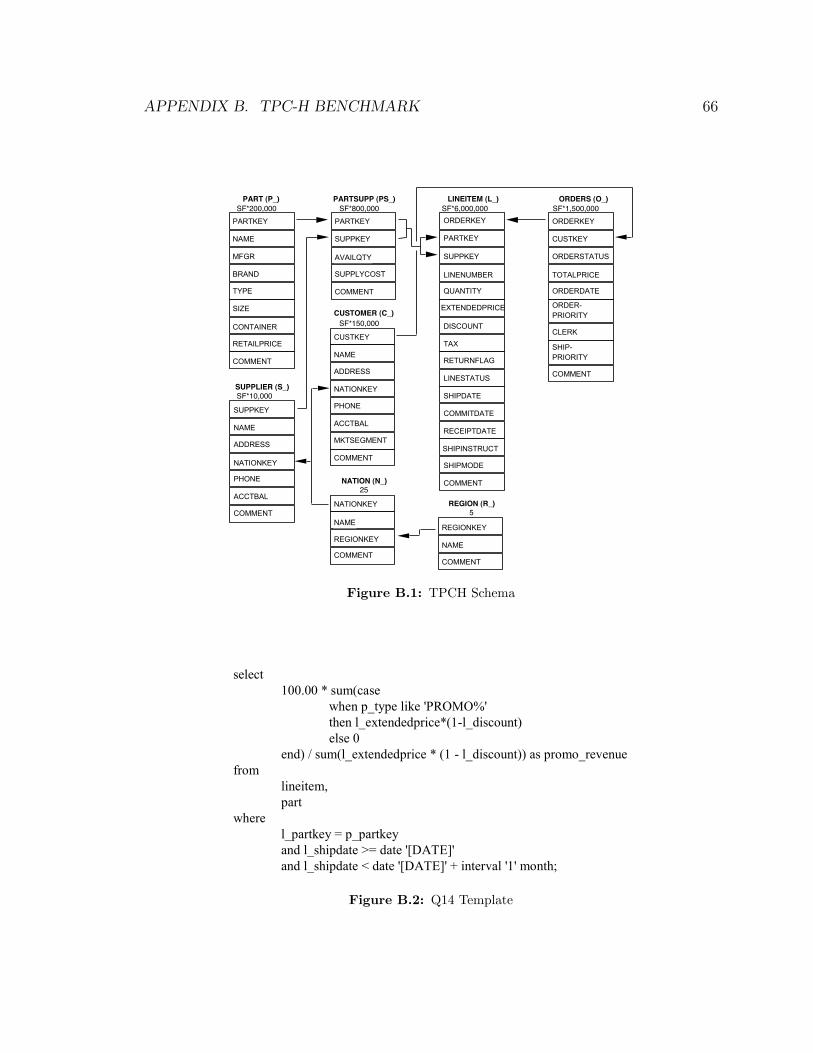
effectiveness of the sort heap usage estimation approach. The TPC-H [20] benchmark
was found to contain suitable queries. TPC-H is a benchmark for OLAP, or business
intelligence, workloads. Queries in this workload perform data analysis tasks resulting
in complex query plans with many operations. TPC-H consists of 22 queries. Of these
22 queries, 18 were chosen as suitable for the evaluation of our estimation approach.2
More information on the TPC-H Benchmark can be found in Appendix B.
The sort heap estimation method was tested against two database sizes to ensure
its flexibility. One database was created with TPC-H scale factor 1—small database,
approx. 1GB—and another database with TPC-H scale factor 3—large database,
approx. 3 GB. Benchmark Factory [21] was used to build these databases. Benchmark
2Queries 9, 15, 17 and 20 were excluded from the evaluations for reasons such as requiring thecreation a view, which our estimation approach does not consider, and extremely long run timewithout any sort heap usage.
CHAPTER 3. ESTIMATING RESOURCE DEMAND 27
Factory for databases is a performance testing tool that helps conduct industry-
standard benchmark testing. However, for our purposes we only borrow the tool’s
database building capabilities. The database system that was used was DB2 V9.7 [12],
installed on Windows Server Professional 2008 on a machine with a quad-core CPU
and 8GB RAM. The data was striped across two disks. The bufferpools of both
databases were configured to be able to hold all the tables in order eliminate I/O
contention in our machine due to the availability of limited disk.
DB2 Sort Heap Parameters
DB2 9.7 has two parameters that affect the available sort heap for a database;
sortheap cfg and sheapthres shr. As mentioned in Section 3.3, sortheap cfg restricts
the amount of sort heap that a single operation can allocate. The other parameter,
shsortheap thres, limits the total amount of sort heap that can be allocated by all
queries running in the database at one time. In recent versions of the DB2 database
system, sortheap cfg and shsortheap thres adjust dynamically, which means their val-
ues change as needed. In order to make external prediction of sort heap usage feasible,
this feature was disabled, and static values were set. However, the same concepts and
conclusions apply to systems with dynamically adjusting values, the current values
of sortheap cfg and shsortheap thres would be used to estimate sort heap usage.
For the evaluation of the estimation approach, three different sort heap configu-
rations were used which are summarized in Table 3.1. Each of these sort heap con-
figurations was used on both the small and large database, for a total of 6 different
configurations.
CHAPTER 3. ESTIMATING RESOURCE DEMAND 28
sortheap cfg sheapthres shr
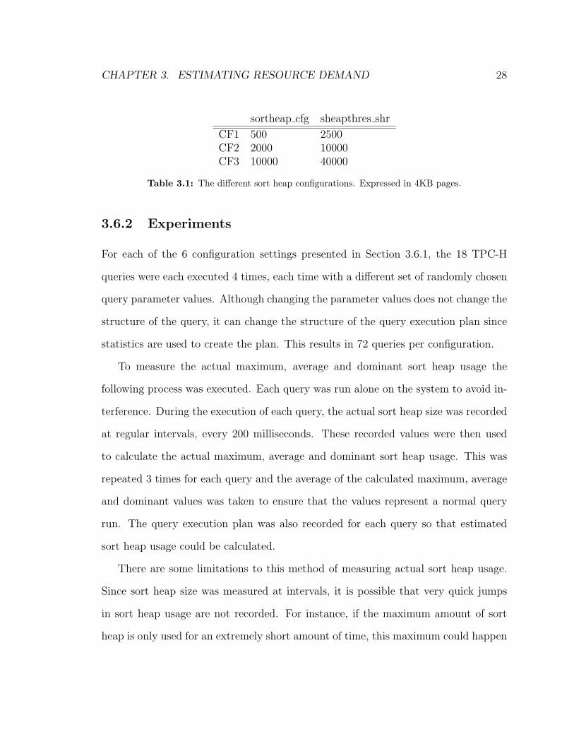
CF1 500 2500CF2 2000 10000CF3 10000 40000
Table 3.1: The different sort heap configurations. Expressed in 4KB pages.
3.6.2 Experiments
For each of the 6 configuration settings presented in Section 3.6.1, the 18 TPC-H
queries were each executed 4 times, each time with a different set of randomly chosen
query parameter values. Although changing the parameter values does not change the
structure of the query, it can change the structure of the query execution plan since
statistics are used to create the plan. This results in 72 queries per configuration.
To measure the actual maximum, average and dominant sort heap usage the
following process was executed. Each query was run alone on the system to avoid in-
terference. During the execution of each query, the actual sort heap size was recorded
at regular intervals, every 200 milliseconds. These recorded values were then used
to calculate the actual maximum, average and dominant sort heap usage. This was
repeated 3 times for each query and the average of the calculated maximum, average
and dominant values was taken to ensure that the values represent a normal query
run. The query execution plan was also recorded for each query so that estimated
sort heap usage could be calculated.
There are some limitations to this method of measuring actual sort heap usage.
Since sort heap size was measured at intervals, it is possible that very quick jumps
in sort heap usage are not recorded. For instance, if the maximum amount of sort
heap is only used for an extremely short amount of time, this maximum could happen
CHAPTER 3. ESTIMATING RESOURCE DEMAND 29
between intervals and not be recorded, resulting in an inaccurate maximum sort heap
usage measurement. However, since the sort heap is being measured several times
a second and sorts and hash joins are operations that typically take longer than
this, it is unlikely that any significant changes in sort heap usage occur between the
measurment intervals.
3.6.3 Results
Once all the queries for all the configurations were run, the results were filtered.
Queries whose execution time was too short (less than 5 data points) to produce
accurate real statistics were eliminated. Furthermore, queries that used no or in-
significant amounts of sort heap (less than 30 4KB pages) were filtered out to avoid
superior results due to trivial cases of predicting that a query requires no sort heap.
After filtering, 301 query runs remained, approximately 50 runs per configuration. To
measure the accuracy of the estimations, percent error was calculated for each metric
(maximum, average and dominant) for each query.
percentError =measuredV alue− estimatedV alue
measuredV alue
The average percent error, standard deviation and median percent error for each
configuration are shown in Table 3.2. The box plots in Figure 3.3 visually display
the distribution of percent error values for all 301 queries. The bold line in each of
the graphs indicates the median percent error, the lower line of the box indicates the
1st quartile, the upper line of the box indicates the 3rd quartile. The surrounding
lines show the lowest value within 1.5 times the inter quartile range (IQR) of the 1st
quartile, and the highest value within 1.5 IQR of the 3rd quartile.
CHAPTER 3. ESTIMATING RESOURCE DEMAND 30
●
●
●●
●
●
●●
020
4060
80
(a) MAX
●●
●
●
●
●
●
●
●
●
●
●
●
●●
●
050
100
150
(b) AVERAGE
●
●
●
●●
●
●
●●
●
●●
●●●
●
●
●
●
●
●●●
●●●●●●
●
●●
●●●●
050
100
150
(c) DOMINANT
Figure 3.3: Box plots showing the distribution of percent error values for the estimation ofthe different sort heap metrics.
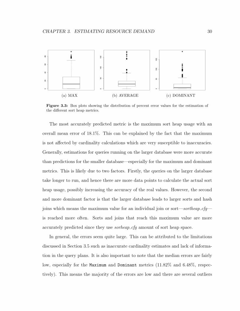
The most accurately predicted metric is the maximum sort heap usage with an
overall mean error of 18.1%. This can be explained by the fact that the maximum
is not affected by cardinality calculations which are very susceptible to inaccuracies.
Generally, estimations for queries running on the larger database were more accurate
than predictions for the smaller database—especially for the maximum and dominant
metrics. This is likely due to two factors. Firstly, the queries on the larger database
take longer to run, and hence there are more data points to calculate the actual sort
heap usage, possibly increasing the accuracy of the real values. However, the second
and more dominant factor is that the larger database leads to larger sorts and hash
joins which means the maximum value for an individual join or sort—sortheap cfg—
is reached more often. Sorts and joins that reach this maximum value are more
accurately predicted since they use sorheap cfg amount of sort heap space.
In general, the errors seem quite large. This can be attributed to the limitations
discussed in Section 3.5 such as inaccurate cardinality estimates and lack of informa-
tion in the query plans. It is also important to note that the median errors are fairly
low, especially for the Maximum and Dominant metrics (11.82% and 6.48%, respec-
tively). This means the majority of the errors are low and there are several outliers
CHAPTER 3. ESTIMATING RESOURCE DEMAND 31
with very high error values. This is also evident in the box plots. Furthermore, since
the estimated values are summaries of a query’s sort heap usage curve, a high degree
of accuracy is not crucial. Because of the nature of a sort heap usage curve, the actual
sort heap usage will vary from any predicted value for much of its execution anyways.
The estimations are required to give a rough idea of how much sort heap the query
requires. This can be achieved even with an error of 20%. Chapter 4 verifies this by
successfully scheduling queries using the proposed sort heap estimation method.
The Blocking Queue Scheduler’s functionality consists solely of gatekeeping. All the
queries that enter the system are put in a queue in the order they arrived. The query
at the front of the queue is only executed if there is enough sort heap space for it. It
follows a first-in-first-out (FIFO) policy. If there is not enough space, the scheduler
waits until enough space is available. The advantages of this scheduler are that it is
very simple to implement, there is very little overhead, and the issue of starvation—
when a query is never executed—is avoided. The main disadvantage is that it is not
flexible in terms of being able to pick which query runs next. There may be a query
CHAPTER 4. LOAD CONTROL SYSTEM 37
in the queue for which there is enough sort heap space available, but it cannot be run
until it is at the front of the queue.
“Smallest” Job First Scheduler (SJFS)
An alternative to the FIFO policy is a shortest-job-first policy. We modify this policy
to a smallest-job-first policy. This means ordering the incoming queries by their sort
heap requirements—from smallest to largest—and then performing gate keeping just
like the Blocking Queue Scheduler. The advantage of this approach is that if a query
fits into the currently available sort heap, it will be allowed to run.1 However, this
type of scheduling induces more overhead than BQS since the waiting queries need
to be sorted. Also, there is the risk of starvation since queries are re-ordered when
new ones arrive.
First Fit Scheduler (FFS)
The First Fit Scheduler keeps a list of all the queries that have been submitted to the
system in the order they were submitted. It traverses through this list until a query
whose sort heap requirement is less than or equal to the currently available sort heap
space is found. Once found, the query is executed and removed from the list. Then,
the search for the next query to execute is repeated from the beginning of the list. A
first-fit approach was chosen rather than a best-fit since the available sort heap space
is constantly changing; by the time the best-fit query is found, it may no longer be
the best fit. Therefore, the extra overhead involved in finding the best fit brings little
1Only the first query is considered for execution, but since this query is the one requiring theleast sort heap, either there will be space for it and it will be allowed to execute or there will notbe enough space for it, which means there is not enough space for any of the other waiting querieseither, since they all require more sort heap.
CHAPTER 4. LOAD CONTROL SYSTEM 38
benefit.
The advantage of this scheduler is that, like SJFS, if there is a query for which
there is enough sort heap space, it will be executed. However, FFS is more likely
to run a balanced mix of queries than SJFS, since queries of all sizes are considered
for execution, not just the one requiring the least sort heap. Nevertheless, of all the
proposed schedulers, FFS is the one that requires the largest overhead since the list
of waiting queries is constantly traversed. This is not a problem as long as long as the
list of waiting queries is small. However, under very heavy loads the waiting query
list could get very long. In these cases, overhead could be reduced by only considering
the first n queries in the list. This way, the overhead of searching for the next query
to execute is constant, no matter how heavy the workload. FFS is also susceptible to
starvation.
4.3 Experimental Environment
In order to assess the effectiveness of each of the proposed scheduling methods, a
prototype external load control system was implemented. An overview of this system
is shown in Figure 4.1. Clients send their requests directly to the load control system
which then retrieves the query execution plan for the request from DBMS. This plan is
then analyzed using the methods described in Chapter 3 to determine the sort heap
requirement of the request. The scheduling system uses this information, the sort
heap model described in Section 4.1 and the chosen scheduling method to determine
when to forward each request to the database system.
Because the load control system is external, it adds overhead to the execution of
the workload. We attempt to minimize the overhead as much as possible, however,
CHAPTER 4. LOAD CONTROL SYSTEM 39
Client
DB2
Query Queue
Sort Heap Req. Estimator
Sort Heap Model
Load Control System
Scheduler
Figure 4.1: Architecture of the Load Control System.
some operations are still very costly. The largest portion of the overhead is incurred
by retrieving the query plans. This involves querying the DBMS to get the plan, which
is written to a file, this file is then parsed by the load control system to extract the
query plan. Furthermore, maintaining the sort heap model also causes overhead since
the database is regularly queried to obtain the current actual size of the sort heap.
Another source of overhead is the query queue, which is implemented by a linked
list. The overhead of this queue varies with the scheduling approach. For instance,
since SJFS requires the queries to be in sorted order, a priority queue is used, where
the priority of a query is defined through its sort heap requirement. However, this
overhead of maintaining the query queue is minimal when compared to the overhead
of retrieving the query plans.
The database system, DB2 V9.5, was on a dedicated database server machine.
This server machine contained 8GB of RAM, a quad core CPU and ran Windows
Server 2008. The clients and load control system were run on a separate machine
CHAPTER 4. LOAD CONTROL SYSTEM 40
running Windows 7, with 2GB RAM and a dual core CPU.
The workload consisted of 12 clients, each running the 18 TPC-H queries intro-
duced in Section 3.6.1. Each client submitted the 18 queries in a different order which
was chosen randomly before the first run and then kept constant throughout all the
workload runs. The database which the queries were run against was the larger of
the two databases introduced in Section 3.6.1. Again, the bufferpool was configured
to be large enough to contain all of the relevant tables. Three different sort heap
configurations were used. These are listed in Table 4.1.
sortheap cfg sheapthres shr
CF1 500 2500CF2 2000 10000CF3 10000 40000
Table 4.1: The different sort heap configurations. Expressed in 4KB pages.
Note that sort heap configurations CF1 and CF2 cap the sort heap that a sin-
gle operation is allowed to use at a relatively low level, 500 and 2000 4KB pages
respectively. This means that many queries will use this maximum, or a multiple of
it, which leads to the variety of sort heap requirements among queries being rather
restricted. CF3 caps the amount of sort heap a single operation is allowed to use
at a higher level, namely 10,000 4KB pages. Few operations in our workload reach
this maximum and thus there is a wider spread of sort heap requirements. In other
words, when considering a set of queries under CF1 or CF2, these queries are likely
to have more homogeneous sort heap requirements than if they were under CF3.
From a scheduling point of view, having a wider spread in sort heap requirements is
favourable since it is more likely that a query whose sort heap requirements matches
the current availability exists.
CHAPTER 4. LOAD CONTROL SYSTEM 41
For each combination of sort heap configuration, scheduling approach and sort
heap model, the workload was run eight times. Before each run, the database system
was restarted to clear all the monitor elements and a sample load was run to fill
the bufferpool with data and bring the database into a steady state. In addition to
the proposed scheduling approaches, the workload was also run with no control, and
with different multiprogramming levels. Running the workload without any control
provides a base from which to compare the scheduling methods. However, it is not
sufficient to compare the proposed scheduling techniques to running the workload
without any control. Without any control, the workload overloads not only the sort
heap but also many other system resources. Since the proposed schedulers limit con-
currency, the load on all resources is reduced. Therefore, comparing the schedulers
to no control does not reflect whether gains in performance are due to being able
to effectively control sort heap usage. Comparing the schedulers to the use of static
MPLs is a much fairer comparison. This comparison determines if strategically se-
lecting when to run which queries is more effective than simply reducing the number
of concurrent queries. It was discovered experimentally that performance, in terms
of total execution time, of the chosen workload peaks around MPL 4. Therefore,
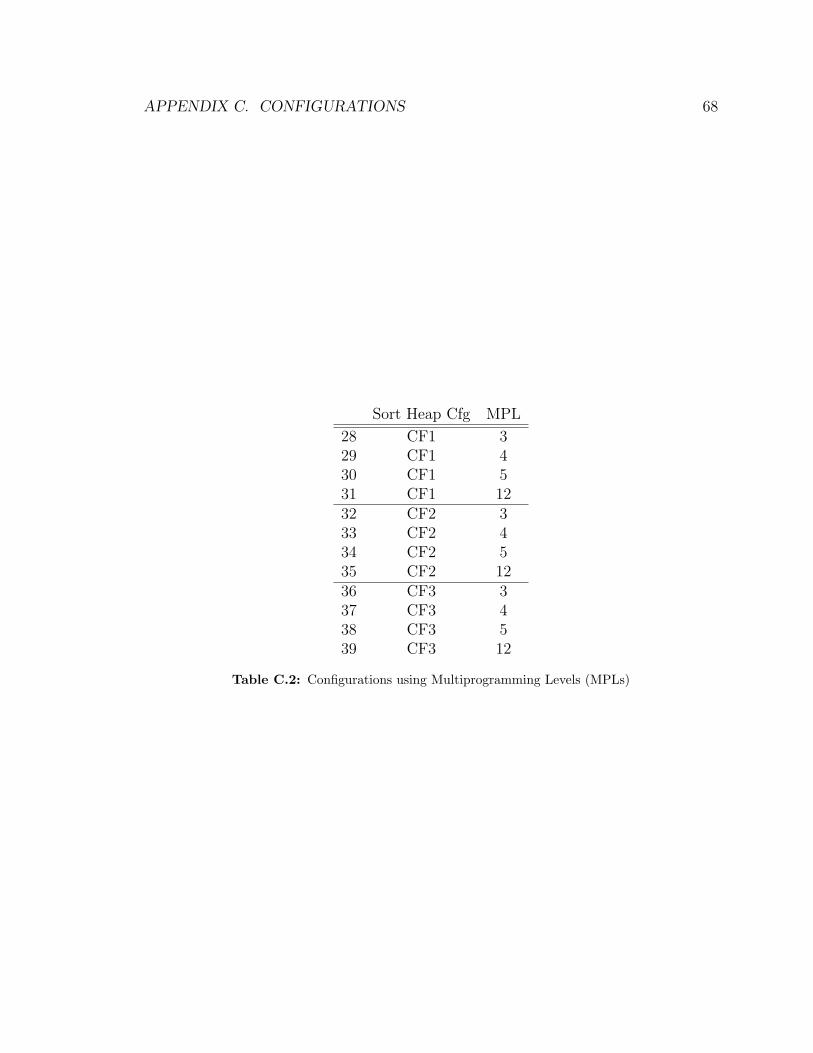
the workload was run with MPLs 3, 4 and 5. Appendix C lists all the different con-
figurations, consisting of a combination of scheduling technique or MPL, sort heap
configuration and sort heap model, for which experiments were performed.
The evaluation of the scheduling methods is presented in two parts. Firstly, the
effectiveness of the scheduling methods is presented in terms of their ability to control
sort heap usage and compared to the use of an MPL (see Section 4.4). Secondly, the
scheduling methods are compared to each other from a user’s point of view (see
CHAPTER 4. LOAD CONTROL SYSTEM 42
Section 4.5).
4.4 Evaluation of Sort Heap Contention Control
4.4.1 Evaluation Metrics
While the goal of our load control system is to control contention on the sort heap, it
is also important to consider the effect this control has on the overall performance of
the system. Overall performance can be measured in terms of total execution time,
which is the elapsed time from when the workload is started to when it completes
(when the last query is finishes). Simply reducing contention on the sort heap is a
trivial task; it can be achieved by reducing the concurrency level. Running one query
at a time will produce the least contention on the sort heap. However, doing this leads
to a longer total execution time. The challenge lies in reducing sort heap contention
while maintaining a level of concurrency necessary to achieve a near optimal total
execution time. Therefore, when comparing scheduling methods to each other and
to the use of static MPLs, we not only consider sort heap contention, but also total
execution time.
We measure sort heap contention by looking at sort heap monitor elements. These
are values which the database tracks and can be accessed externally through database
snapshots. The specific elements are listed in Table 4.2. Post-threshold operations are
an indicator of sort heap contention because they occur when sort heap memory is at
its capacity or close to capacity. Therefore, an increase in post-threshold operations
means that contention on the sort heap has increased. Post-threshold operations
should be avoided since they lead to poor performance. A post-threshold sort or
CHAPTER 4. LOAD CONTROL SYSTEM 43
hash join will take longer to complete than the same sort or hash join without the
post-threshold status because it must complete using a less than optimal amount of
memory, which can result in having to write partial results to disk. Because of this,
total sort time and the number of post-threshold sorts are closely related.
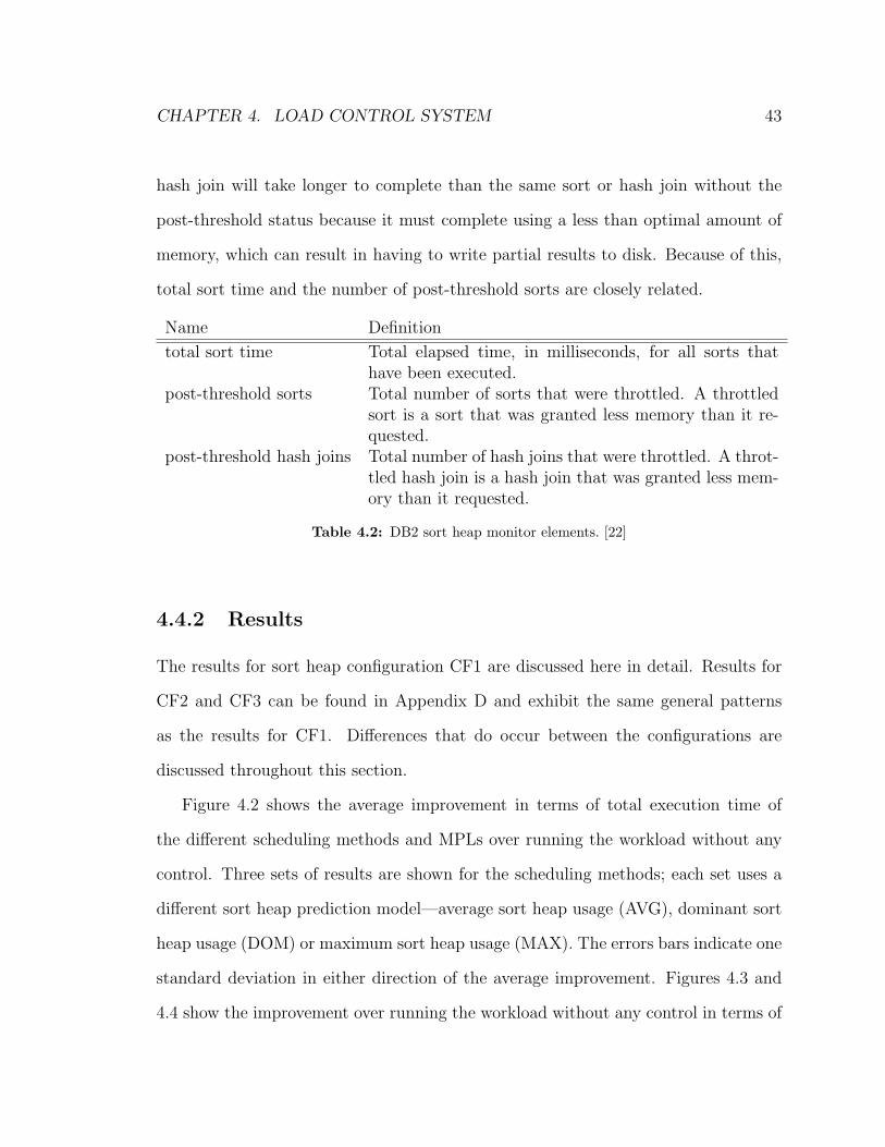
Name Definition
total sort time Total elapsed time, in milliseconds, for all sorts thathave been executed.
post-threshold sorts Total number of sorts that were throttled. A throttledsort is a sort that was granted less memory than it re-quested.
post-threshold hash joins Total number of hash joins that were throttled. A throt-tled hash join is a hash join that was granted less mem-ory than it requested.
Table 4.2: DB2 sort heap monitor elements. [22]
4.4.2 Results
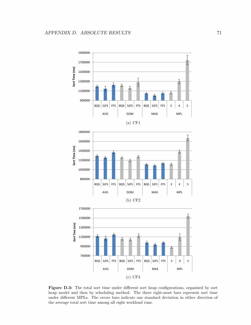
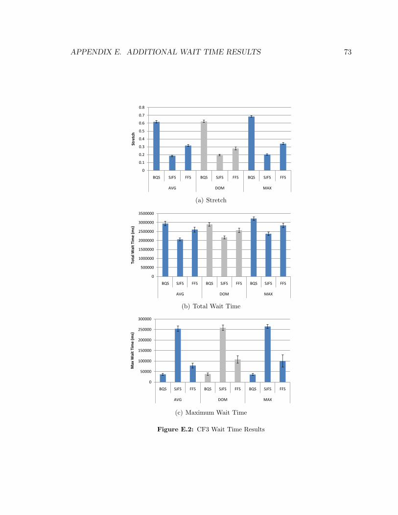
The results for sort heap configuration CF1 are discussed here in detail. Results for
CF2 and CF3 can be found in Appendix D and exhibit the same general patterns
as the results for CF1. Differences that do occur between the configurations are
discussed throughout this section.
Figure 4.2 shows the average improvement in terms of total execution time of
the different scheduling methods and MPLs over running the workload without any
control. Three sets of results are shown for the scheduling methods; each set uses a
heap usage (DOM) or maximum sort heap usage (MAX). The errors bars indicate one
standard deviation in either direction of the average improvement. Figures 4.3 and
4.4 show the improvement over running the workload without any control in terms of
CHAPTER 4. LOAD CONTROL SYSTEM 44
0
10
20
30
40
50
60
BQS SJFS FFS BQS SJFS FFS BQS SJFS FFS 3 4 5
AVG DOM MAX MPL
Total Execution Tim
e
(% Im
provement)
Figure 4.2: Percent improvement in total execution time over running the workload with nocontrol.
50
60
70
80
90
100
110
BQS SJFS FFS BQS SJFS FFS BQS SJFS FFS 3 4 5
AVG DOM MAX MPL
Post-‐thresho
ld Ope
ratio
ns
(% Im
prov
emen
t)
Figure 4.3: Percent improvement in total sort time over running the workload with no control.
50
55
60
65
70
75
80
85
BQS SJFS FFS BQS SJFS FFS BQS SJFS FFS 3 4 5
AVG DOM MAX MPL
Total Sort Tim
e
(% Im
provement)
Figure 4.4: Percent improvement in the number of post-threshold operations over running theworkload with no control.
CHAPTER 4. LOAD CONTROL SYSTEM 45
number of post-threshold operations and total sort time, respectively. The absolute
results can be found in Appendix D.
First, let us compare the sort heap models to each other. Using the AVG or DOM
sort heap model leads to greater improvement in total execution time than using
the MAX model (5.2% to 7.9% greater improvement). This can be explained by the
fact that using the maximum sort heap estimation is a very conservative approach
that may unnecessarily limit the concurrency level. Generally there is little difference
(less than 1.4%) between using the AVG and DOM sort heap models with respect
to improvement in total execution time. However, the MAX sort heap model leads
to greater improvement in both the number of post-threshold operations (2.3% to
5.3%) and total sort time (3.0% to 5.0%). This can again be attributed to the fact
that the MAX model is the most restrictive since the worst case is always assumed;
that a query will always use its maximum amount of sort heap memory. Therefore,
contention on the sort heap is low which means less post-threshold operations.
The difference between using a MAX model over a DOM or AVG model in terms
of total execution time, which is very observable under CF1, becomes less dominant
under CF2 and even more so under CF3. This is likely due to the fact that queries
have more varied sort heap requirements under CF2 and CF3, which means that a
query that fits into the available sort heap can be found more often and more queries
can be executed concurrently. Although the difference in execution time changes with
the sort heap configuration, the MAX model consistently leads to the least number
of post threshold operations and least amount of sort time.
In terms of comparing the different scheduling approaches, BQS and FFS show
greater improvement in terms of total execution time than SJFS (0.8% to 3.0%).
CHAPTER 4. LOAD CONTROL SYSTEM 46
This is likely due to the fact that SJFS overloads the system on resources other than
the sort heap since it does not execute a balanced mix of queries. In fact, SJFS is
the scheduling method which causes the least sort heap contention (SJFS exhibits
the greatest improvement in post-threshold operations and total sort time) which is
evident in Figures 4.3 and 4.4.
The scheduling approaches are not always superior to a well-chosen MPL in terms
of improvement in total execution time. However, the schedulers are generally more
effective in reducing the number of post-threshold operations and sort time while
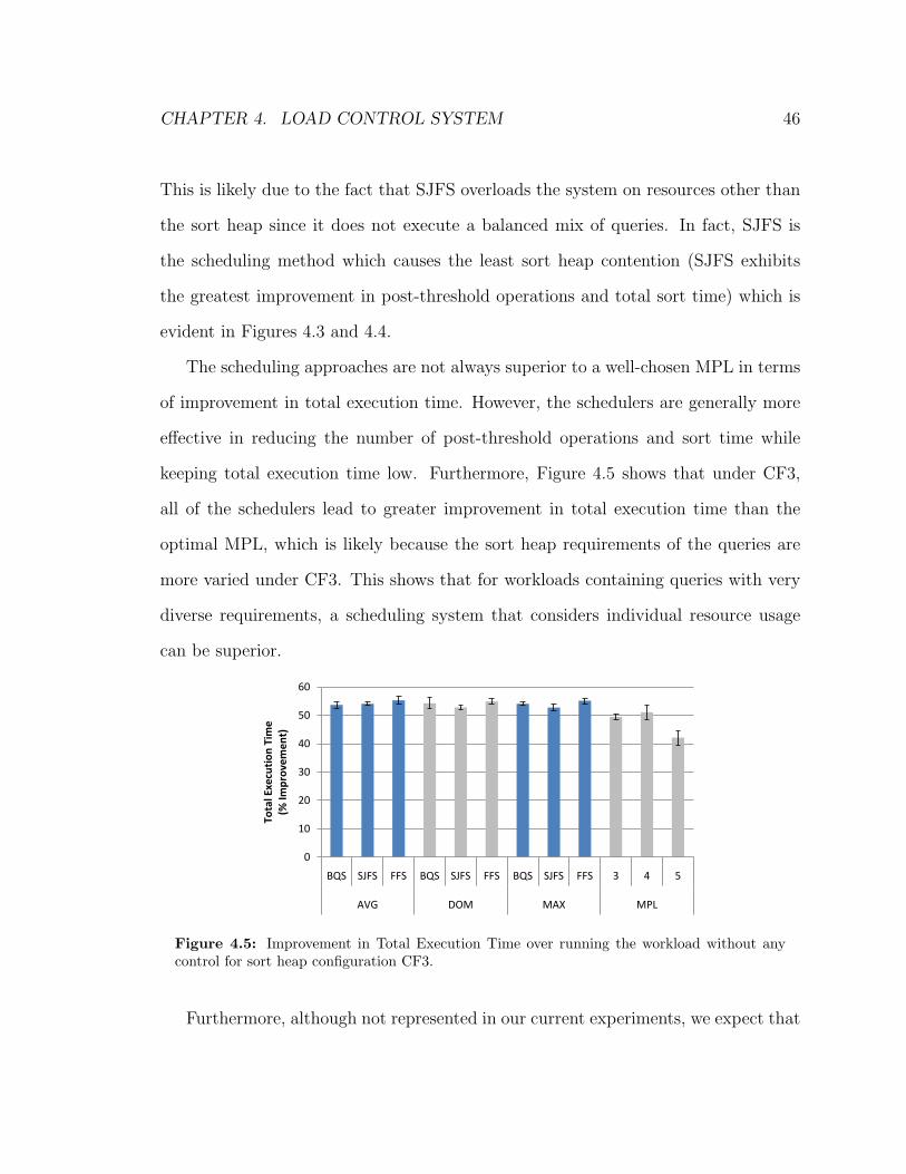
keeping total execution time low. Furthermore, Figure 4.5 shows that under CF3,
all of the schedulers lead to greater improvement in total execution time than the
optimal MPL, which is likely because the sort heap requirements of the queries are
more varied under CF3. This shows that for workloads containing queries with very
diverse requirements, a scheduling system that considers individual resource usage
can be superior.
0
10
20
30
40
50
60
BQS SJFS FFS BQS SJFS FFS BQS SJFS FFS 3 4 5
AVG DOM MAX MPL
Total Execution Tim
e
(% Im
provement)
Figure 4.5: Improvement in Total Execution Time over running the workload without anycontrol for sort heap configuration CF3.
Furthermore, although not represented in our current experiments, we expect that
CHAPTER 4. LOAD CONTROL SYSTEM 47
under a changing workload, our load control system is superior to the use of an MPL.
Since the best MPL is determined experimentally for the given workload, it may not
be the best MPL for a different workload. Under a different workload, the MPL
will either have to be adjusted or the system will perform poorly. However, our load
control system works in a predictive manner, and therefore will be able to adjust
automatically to the changing workload. If the queries arriving in the system require
a different set of resources, then the system will schedule them so that the required
resources still match the available resources. We plan to investigate this in future
experiments (see Section 5.2).
4.5 Evaluation of the Scheduling Techniques
4.5.1 Evaluation Criteria
While the scheduling approaches are all fairly similar in their ability to control sort
heap contention, there is a difference in the way they schedule queries. BQS executes
queries in the order in which they were submitted, while SJFS and FFS change this
order. Changing the order in which queries are submitted can lead to long wait times
for some queries. From a system efficiency point of view, it does not matter which
queries are being executed as long as resources are being used well and throughput
is high. However, the users submitting the queries see this differently. A user who
submits a query to the system expects a response within a reasonable amount of time.
In this Section, we compare the scheduling approaches and sort heap models in terms
of their effect on wait time. Wait time for a query is the elapsed time from when the
query was submitted to when it starts executing. By examining different wait time
CHAPTER 4. LOAD CONTROL SYSTEM 48
metrics, we can compare the different scheduling approaches from a user’s point of
view.
One way to evaluate wait time is to look at the stretch metric [23]. Stretch
expresses the relationship between a query’s wait time and execution time. The main
idea is that a user who submits a long query is willing to wait longer than a user who
submits a very short query. The stretch of a query q is defined as,
stretchq =wq + eq
eq
(4.5)
where wq is the wait time of q and eq is the execution time of q. In addition to stretch
we also use maximum wait time (the maximum amount of time a query had to wait)
and total wait time (the sum of the individual wait times for each query) to compare
the scheduling techniques.
4.5.2 Results
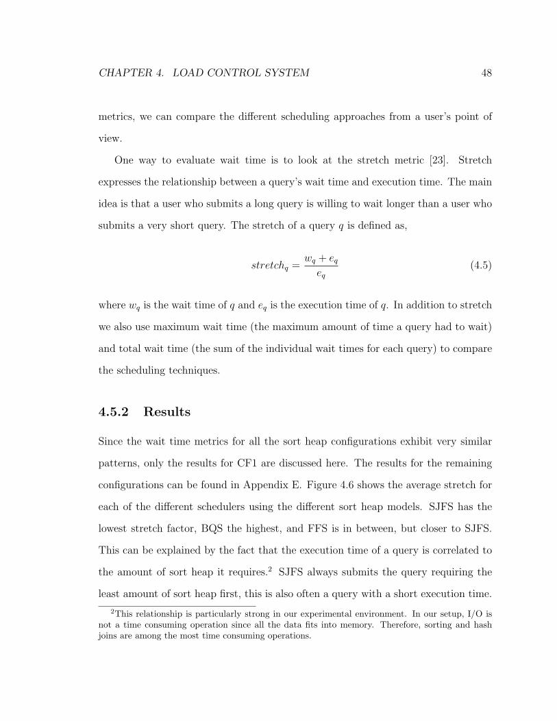
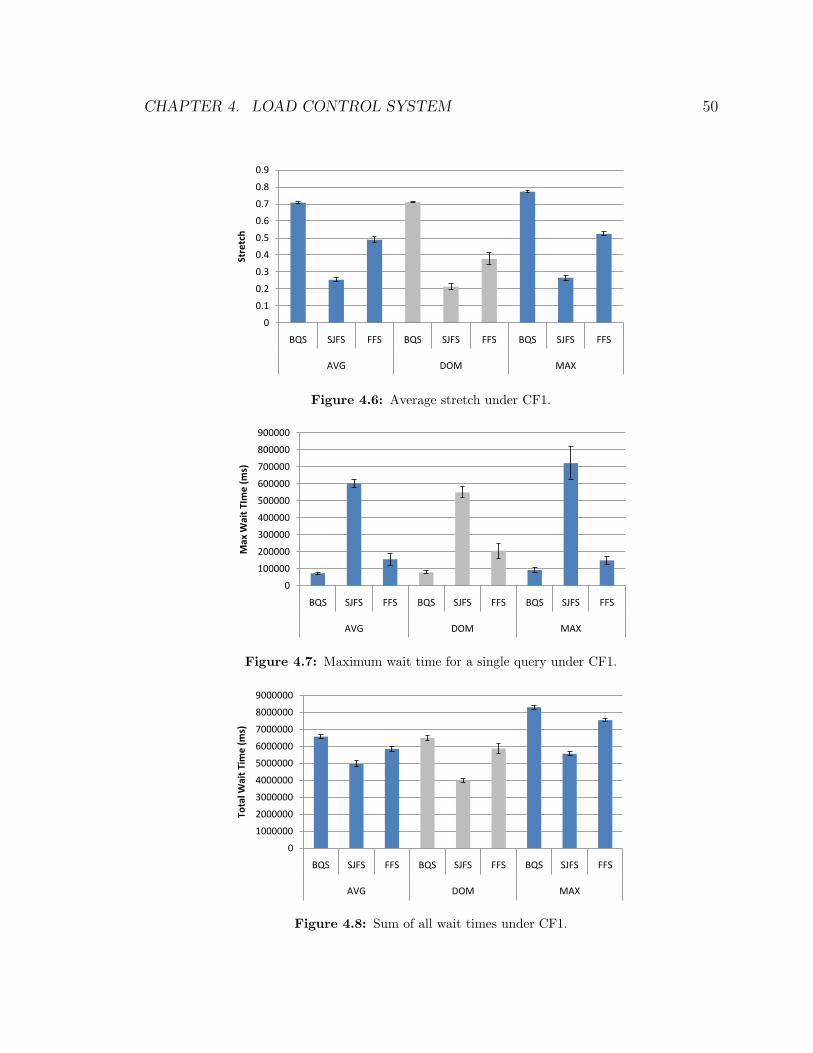
Since the wait time metrics for all the sort heap configurations exhibit very similar
patterns, only the results for CF1 are discussed here. The results for the remaining
configurations can be found in Appendix E. Figure 4.6 shows the average stretch for
each of the different schedulers using the different sort heap models. SJFS has the
lowest stretch factor, BQS the highest, and FFS is in between, but closer to SJFS.
This can be explained by the fact that the execution time of a query is correlated to
the amount of sort heap it requires.2 SJFS always submits the query requiring the
least amount of sort heap first, this is also often a query with a short execution time.
2This relationship is particularly strong in our experimental environment. In our setup, I/O isnot a time consuming operation since all the data fits into memory. Therefore, sorting and hashjoins are among the most time consuming operations.
CHAPTER 4. LOAD CONTROL SYSTEM 49
Hence, the query’s wait time is proportional to its execution time. When SJFS is
used, queries that require a very large amount of sort heap get stuck at the end of
the queue and may have to wait a long time before being executed, however, these
queries also take longer to execute and hence the relationship between wait time and
execution time remains proportional.
Total wait time is shown in Figure 4.8 and maximum wait time for a single query
is shown in Figure 4.7. While SJFS is also superior to the other schedulers in terms
of total wait time, it produces much longer maximum wait times. This is due to the
fact that queries requiring large amounts of sort heap can become ‘stuck’ at the end
of the queue.
The best choice of scheduling method very much depends on the workload. If the
workload is a batch workload (a set of queries to be completed as a whole), then SJFS
is a good choice, since it minimizes total wait time and the fact that some queries
may have to wait a very long time does not matter. However, if the type of workload
is continuous, SJFS should be avoided. If new queries are continually entering the
system, then enough resources for the large queries at the end of the queue may never
become available. In this case BQS may be the best choice, because it cannot lead to
starvation. However, FFS is generally better at balancing sort heap usage and total
execution time. Section 4.6 presents a modified version of FFS which eliminates the
risk of starvation.
4.6 Avoiding Starvation
A significant drawback to re-ordering queries when scheduling is the possibility of
starvation and very long wait times. In order to address this issue, we present an
CHAPTER 4. LOAD CONTROL SYSTEM 50
0
0.1
0.2
0.3
0.4
0.5
0.6
0.7
0.8
0.9
BQS SJFS FFS BQS SJFS FFS BQS SJFS FFS
AVG DOM MAX
Stretch
Figure 4.6: Average stretch under CF1.
0
100000
200000
300000
400000
500000
600000
700000
800000
900000
BQS SJFS FFS BQS SJFS FFS BQS SJFS FFS
AVG DOM MAX
Max W
ait TIme (ms)
Figure 4.7: Maximum wait time for a single query under CF1.
0
1000000
2000000
3000000
4000000
5000000
6000000
7000000
8000000
9000000
BQS SJFS FFS BQS SJFS FFS BQS SJFS FFS
AVG DOM MAX
Total W
ait Time (ms)
Figure 4.8: Sum of all wait times under CF1.
CHAPTER 4. LOAD CONTROL SYSTEM 51
altered version of the First Fit Scheduler. To guarantee that a query will be executed
eventually, that query’s sort heap requirement must eventually fit into the available
sort heap space. To achieve this, the sort heap requirement of a query was redefined
to include a function ScaleFactor(q, t), which scales the sort heap requirement of the
Two possible scale functions were investigated; one which only affects a single
query at a time, and one which affects multiple queries at a time. The first will
be referred to as Single Scale Factor (SFs) and the second as Multiple Scale Factor
(SFm).
ScaleFactor(q, t) =
SFs(q, t)
SFm(q, t)
(4.7)
Both scale factors are dependent on the queries that have been allowed to run up
until time point t. Every time a query q′ that was submitted after q is allowed to
execute, ScaleFactor(q, t) may be affected. Let QRqt be the set of all queries that
have been allowed to run at time point t but which were submitted after query q.
Conceptually, QRqt is the set of all queries that have “jumped” the line in front of
q. Let pq′q be q’s position in the waiting query list at the point in time when query
q′ ∈ QRqt is allowed to run (when pq′q is 0 q is at the front of the list, when pq′
q is 1
q is second in the list, etc.). SFs(q, t), reduces the sort heap requirement of the first
query in the waiting query list by 10%3 every time a query that is not first in line is
3The 10% factor was chosen arbitrarily as a sample value to show the effects of the proposedscaling method. The approach may be optimized by a different choice of scaling factor.
CHAPTER 4. LOAD CONTROL SYSTEM 52
executed.
SFs(q, t) =∏
q′∈QRqt
0.9 if pq′
q is 0
1 otherwise
(4.8)
SFm scales up to the first five queries in the waiting query list in a decreasing
manner, whenever a query is executed.
SFm(q, t) =∏
q′∈QRqt
min{0.9 + pq′
q ∗ 0.02, 1} (4.9)
0
5
10
15
20
25
30
35
40
SFs SFm SFs SFm SFs SFm
CF1 CF2 CF3
Max W
ait Time
(% Im
provement)
Figure 4.9: Reduction in wait time over FFS without scaling.
We chose this method of scaling sort heap requirements instead of a more tradi-
tional time-based aging approach because our goal is to penalize certain scheduling
decisions. We also want to avoid unnecessarily scaling a query’s sort heap require-
ment since this leads to poor performance. Our approach only scales those queries
that have to wait longer than they would have to if queries were not being rearranged.
A time-based approach ages queries independent of scheduling decisions.
The goal of scaling the sort heap requirements of certain queries was to avoid
starvation and extremely long wait times. To see if this was achieved, we examine
CHAPTER 4. LOAD CONTROL SYSTEM 53
the reduction in maximum wait time exhibited by FFS with the two different scaling
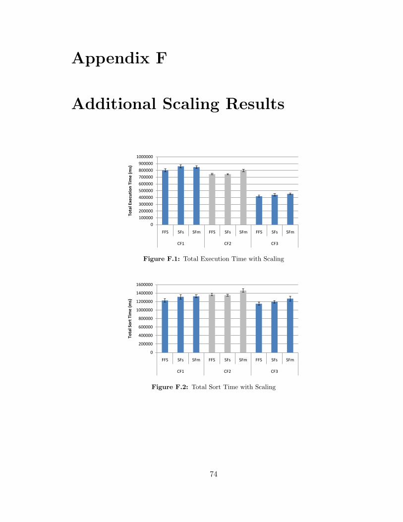
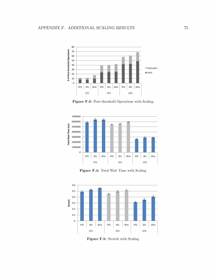
methods over FFS without scaling. Figure 4.9 shows this improvement for each of the
sort heap configurations. The use of SFm leads to greater improvement in maximum
wait times than SFs. However, both gains come at a cost. Essentially all other factors
that were measured, were negatively affected. Scaling the sort heap requirements of
certain queries increases total execution time (up to 8.2%), total sort time (up to
10.5%), the number of post threshold operations (up to 51%), average stretch (up to
28.6%) and total wait time (up to 11.7%). Complete results can be found in Appendix
F. All these metrics were affected less by SFs than by SFm. It is interesting that
scaling, which is done to reduce wait time, negatively affects total wait time. This
is likely because queries that overload the sort heap can be chosen to execute, which
slows down the system and other queries have to wait longer than they would have
to if the system was running efficiently.
Chapter 5
Conclusions and Future Work
As DBMS workloads are becoming more complex, effective load management sys-
tems are needed. Resource-aware load management systems are one way to handle
the varying resource requirements of queries. The objective of this thesis is to inves-
tigate the feasibility of a database load control system based on regulating resource
consumption in a predictive manner. This is accomplished through a proof-of-concept
study focusing on a single resource; namely, the sort heap. Two main contributions
are presented: a method of estimating a query’s sort heap usage and a prototype load
control system implementing three different scheduling methods.
The estimation of a query’s sort heap usage is based on its execution plan. Since
sort heap usage is not constant throughout a query’s execution, it is summarized using
one of three metrics; maximum, average and dominant sort heap usage. It is possible
to calculate these metrics by examining the operators in the query execution plan
and their relationships. First, the amount of sort heap that each operator requires
individually is calculated and then sets of operators that can be active at the same
time are determined.
The prototype load control system consists of three parts: a sort heap model to
track sort heap usage, an estimation module to estimate the sort heap requirements
54
CHAPTER 5. CONCLUSIONS AND FUTURE WORK 55
of incoming queries and a scheduling module to determine when to execute which
queries. The three proposed scheduling methods, in order of increasing overhead, are
as follows: Blocking Queue Scheduler (BQS), Smallest Job First Scheduler (SJFS)
and First Fit Scheduler (FFS). BQS retains the order in which the queries are sub-
mitted and acts solely as a gatekeeping mechanism, only letting the next query run
if there is sufficient sort heap space. SJFS sorts incoming queries by their sort heap
requirements. FFS continually traverses the list of waiting queries and executes those
that fit into the currently available sort heap space. A modified version of FFS which
reduces maximum wait time by scaling sort heap requirements is also presented.
5.1 Conclusions
A comparison of estimated sort heap usage to actual sort heap usage produced the
following mean percent error values: 18.1% for the maximum metric, 30.64% for the
average metric, and 20.77% for the dominant metric. While these mean errors seem
large, many of the individual error values are quite low and several outliers cause the
mean error value to rise. Furthermore, a high degree of accuracy is not crucial since
the numbers are summaries of sort heap usage curves and are only required to give
an approximation of how much sort heap a query will require.
Even though the estimations for the maximum metric are most accurate, experi-
ments using these estimations to schedule queries show that using maximum estima-
tions is a very conservative approach which can excessively limit concurrency. Using
the maximum sort heap model consistently leads to the best improvement in number
of post threshold sorts, up to 5.3% more than the other sort heap models. However,
it also leads to up to 7.9% less improvement in total execution time.
CHAPTER 5. CONCLUSIONS AND FUTURE WORK 56
Our experiments with the prototype load control system show that sort heap
usage can be controlled by any of the three proposed scheduling methods. All of the
scheduling approaches are most effective given a workload with very varied sort heap
requirements. The most promising approach is the First Fit Scheduler; it generally
leads to the best overall execution time. Under a workload with diverse sort heap
requirements, FFS leads to an improvement of up to 55.3% in total execution time
over running the workload with no control, compared to an improvement of 51.1%
using the optimal MPL. While this is not a particularly large difference, it is important
to consider that the optimal MPL was chosen experimentally while FFS adjusts the
concurrency level automatically.
SJFS leads to both the lowest stretch and total wait time values. These are im-
portant from a user’s point of view since a user does not want to wait an unreasonable
amount of time for the result of a particular query. However, SJFS causes dramat-
ically higher maximum wait times than the other scheduling approaches. This is
because queries with large sort heap requirements can get stuck at the end of the
queue. Experiments with a modified version of FFS, which incorporates sort heap
requirement scaling, show that maximum wait time can be reduced at the expense of
total execution time.
Overall, we conclude that predictive resource-aware load control is promising,
especially given a workload with diverse resource requirements. We have shown that
it is possible to predict resource requirements with a level of accuracy suitable for
making scheduling decisions. While the abilities of a load control system based on
a single resource are limited, we believe that once more resources are incorporated,
resource-aware scheduling will be highly effective.
CHAPTER 5. CONCLUSIONS AND FUTURE WORK 57
5.2 Future Work
The results of our proof-of concept study open up many opportunities for future work.
Continuing within the scope of this project we see the following as future work. We
would like to continue our experiments with the proposed scheduling methods under
different workloads and specifically, changing workloads. We believe resource-aware
scheduling can be a powerful tool for adapting to workload changes. Furthermore,
since the estimation of sort heap usage can be very inaccurate for some queries, we
would like to explore the possibility of using historical data to identify query types
whose sort heap prediction has been inaccurate in the past. A confidence in the
estimated sort heap requirement can be reported along with the requirement and the
scheduler can judge how seriously to take the estimation based on its confidence.
On a broader scale, we would like to expand our approach beyond the sort heap.
We would like to be able to estimate other resource requirements such as CPU and
incorporate these resource estimations into our load control system. CPU estimates
could be attained through the query execution plan by identifying CPU intensive
operations and their cardinalities. Another approach is to base CPU estimates on
the number of workers assigned to the processing of a query; the more workers, the
more CPU intensive the query is expected to be.
Finally, we would like to consider factors such as service level objectives (SLOs)
and query priorities and investigate how these can be integrated with resource-aware
scheduling. One possibility is to “age” the resource requirement estimates of high
priority queries to make them more likely to be chosen to execute. Another option
is to have several queues of queries, each with different priority levels, and to give
CHAPTER 5. CONCLUSIONS AND FUTURE WORK 58
preference to the queries in high-priority queues when deciding which query to execute
next.
Bibliography
[1] Abhay Mehta, Chetan Gupta, and Umeshwar Dayal. Bi batch manager: a ys-
tem for managing batch workloads on enterprise data-warehouses. In EDBT
’08: Proceedings of the 11th International Conference on Extending Database
Technology, pages 640–651, New York, NY, USA, 2008.
[2] David Hornby, Bill Walker, and Ken Pepple. Consolidation in the Data Cen-
ter: Simplifying IT Environments to Reduce Total Cost of Ownership. Pearson
Education, 2002.
[3] Moonish Badaloo. An examination of server consolidation: trends that can drive
efficiencies and help businesses gain a competitive edge. IBM White Paper,
August 2008.
[4] IBM Software Group. The New Promise of Business Intelligence. White Paper,
2010.
[5] Ron Kohavi, Neal J. Rothleder, and Evangelos Simoudis. Emerging trends in
business analytics. Communications of the ACM, 45:45–48, August 2002.
[6] Surajit Chaudhuri, Raghav Kaushik, and Ravishankar Ramamurthy. When
can we trust progress estimators for sql queries? In Proceedings of the 2005
ACM SIGMOD International Conference on Management of Data, SIGMOD
’05, pages 575–586, New York, NY, USA, 2005.
[7] Gang Luo, Jeffrey F. Naughton, Curt J. Ellmann, and Michael W. Watzke.
Toward a progress indicator for database queries. In Proceedings of the 2004
59
BIBLIOGRAPHY 60
ACM SIGMOD International Conference on Management of Data, SIGMOD
’04, pages 791–802, New York, NY, USA, 2004.
[8] Surajit Chaudhuri, Vivek Narasayya, and Ravishankar Ramamurthy. Estimating
progress of execution for sql queries. In Proceedings of the 2004 ACM SIGMOD
International Conference on Management of Data, SIGMOD ’04, pages 803–814,
The TPC-H Benchmark [20] is a decision support benchmark, developed by the Trans-
action Processing Performance Council. Its main purpose is to be used to evaluate
the performance of decision support systems by executing queries under controlled
conditions. The benchmark consists a set of 22 business oriented ad-hoc queries. The
TPC-H database contains 8 tables. The table names and schemas are shown in Figure
B.1. The size of each of these tables depends on the scale factor (SF). For instance,
with a SF of 1, the PART table contains 800,000 records, with a SF of 5, it contains
4,000,000 records.
Each of the 22 queries is designed to answer a specific business question. For
instance Query 14 answers the following business question:
The Promotion Effect Query determines what percentage of the revenue
in a given year and month was derived from promotional parts. The
query considers only parts actually shipped in that month and gives the
percentage. Revenue is defined as (l extendedprice ∗ (1− l discount)).
The TPC-H specification provides parameterized query templates for all of the
queries Q1 to Q22. The specification defines the allowed value range for each param-
eter. The arguments must then be chosen randomly within this range. Figure B.2
shows the SQL template for Q14. DATE is a parameter which is restricted to being
the first day of a month, randomly selected from a random year between 1993 and
1997.
65
APPENDIX B. TPC-H BENCHMARK 66
TPC BenchmarkTM H Standard Specification Revision 2.14.0 Page 12
1.2 Database Entities, Relationships, and Characteristics
The components of the TPC-H database are defined to consist of eight separate and individual tables (the Base Tables). The relationships between columns of these tables are illustrated in Figure 2: The TPC-H Schema.
F igure 2: The TPC-H Schema
PARTKEY
NAME
MFGR
BRAND
TYPE
SIZE
CONTAINER
COMMENT
RETAILPRICE
PARTKEY
SUPPKEY
AVAILQTY
SUPPLYCOST
COMMENT
SUPPKEY
NAME
ADDRESS
NATIONKEY
PHONE
ACCTBAL
COMMENT
ORDERKEY
PARTKEY
SUPPKEY
LINENUMBER
RETURNFLAG
LINESTATUS
SHIPDATE
COMMITDATE
RECEIPTDATE
SHIPINSTRUCT
SHIPMODE
COMMENT
CUSTKEY
ORDERSTATUS
TOTALPRICE
ORDERDATE
ORDER-PRIORITY
SHIP-PRIORITY
CLERK
COMMENT
CUSTKEY
NAME
ADDRESS
PHONE
ACCTBAL
MKTSEGMENT
COMMENT
PART (P_)SF*200,000
PARTSUPP (PS_)SF*800,000
LINEITEM (L_)SF*6,000,000
ORDERS (O_)SF*1,500,000
CUSTOMER (C_)SF*150,000
SUPPLIER (S_)SF*10,000
ORDERKEY
NATIONKEY
EXTENDEDPRICE
DISCOUNT
TAX
QUANTITY
NATIONKEY
NAME
REGIONKEY
NATION (N_)25
COMMENT
REGIONKEY
NAME
COMMENT
REGION (R_)5
Legend:
The parentheses following each table name contain the prefix of the column names for that table;
The arrows point in the direction of the one-to-many relationships between tables;
The number/formula below each table name represents the cardinality (number of rows) of the table. Some are factored by SF, the Scale Factor, to obtain the chosen database size. The cardinality for the LINEITEM table is approximate (see Clause 4.2.5).
Figure B.1: TPCH Schema
TPC BenchmarkTM H Standard Specification Revision 2.14.0 Page 51
2.4.14 Promotion E ffect Query (Q14) This query monitors the market response to a promotion such as TV advertisements or a special campaign.
2.4.14.1 Business Question The Promotion Effect Query determines what percentage of the revenue in a given year and month was derived from promotional parts. The query considers only parts actually shipped in that month and gives the percentage. Revenue is defined as (l_extendedprice * (1-l_discount)).
2.4.14.2 Functional Query Definition
select 100.00 * sum(case
when p_type like 'PROMO%' then l_extendedprice*(1-l_discount) else 0
end) / sum(l_extendedprice * (1 - l_discount)) as promo_revenue from
lineitem, part
where l_partkey = p_partkey and l_shipdate >= date '[DATE]' and l_shipdate < date '[DATE]' + interval '1' month;
2.4.14.3 Substitution Parameters Values for the following substitution parameter must be generated and used to build the executable query text:
1. DATE is the first day of a month randomly selected from a random year within [1993 .. 1997].
2.4.14.4 Query Validation For validation against the qualification database the query must be executed using the following values for substitu-tion parameters and must produce the following output data: Values for substitution parameters:
Table C.2: Configurations using Multiprogramming Levels (MPLs)
Appendix D
Absolute Results
700000
750000
800000
850000
900000
950000
1000000
BQS SJFS FFS BQS SJFS FFS BQS SJFS FFS 3 4 5
AVG DOM MAX MPL
Total Execution Tim
e (ms)
(a) CF1
600000
650000
700000
750000
800000
850000
900000
BQS SJFS FFS BQS SJFS FFS BQS SJFS FFS 3 4 5
AVG DOM MAX MPL
Total Execution Tim
e (ms)
(b) CF2
300000
350000
400000
450000
500000
550000
600000
BQS SJFS FFS BQS SJFS FFS BQS SJFS FFS 3 4 5
AVG DOM MAX MPL
Total Execution Tim
e (ms)
(c) CF3
Figure D.1: The total execution time for the workload under different sort heap configurations,sort heap models and scheduling methods.
69
APPENDIX D. ABSOLUTE RESULTS 70
0
10
20
30
40
50
60
70
80
90
BQS SJFS FFS BQS SJFS FFS BQS SJFS FFS 3 4 5
AVG DOM MAX MPL
# of Post-‐threshold Ope
ratio
ns
hash joins
sorts
(a) CF1
0
10
20
30
40
50
60
70
80
90
BQS SJFS FFS BQS SJFS FFS BQS SJFS FFS 3 4 5
AVG DOM MAX MPL
# of Post-‐threshold Ope
ratio
ns
hash joins
sorts
(b) CF2
0
10
20
30
40
50
60
70
80
BQS SJFS FFS BQS SJFS FFS BQS SJFS FFS 3 4 5
AVG DOM MAX MPL
# of Post-‐threshold Ope
ratio
ns
hash joins
sorts
(c) CF3
Figure D.2: The number of post-threshold operations under different sort heap configurations,organized by sort heap model and then by scheduling method. The three right-most bars showthe number of post-threshold operations under different MPLs.
APPENDIX D. ABSOLUTE RESULTS 71
900000
1100000
1300000
1500000
1700000
1900000
BQS SJFS FFS BQS SJFS FFS BQS SJFS FFS 3 4 5
AVG DOM MAX MPL
Sort Tim
e (ms)
(a) CF1
800000
1000000
1200000
1400000
1600000
1800000
BQS SJFS FFS BQS SJFS FFS BQS SJFS FFS 3 4 5
AVG DOM MAX MPL
Sort Tim
e (ms)
(b) CF2
700000
900000
1100000
1300000
1500000
1700000
BQS SJFS FFS BQS SJFS FFS BQS SJFS FFS 3 4 5
AVG DOM MAX MPL
Sort Tme (ms)
(c) CF3
Figure D.3: The total sort time under different sort heap configurations, organized by sortheap model and then by scheduling method. The three right-most bars represent sort timeunder different MPLs. The errors bars indicate one standard deviation in either direction ofthe average total sort time among all eight workload runs.