Resource Factors Affecting Labour Demand forTextile … Resource Factors Affecting Labour Demand...

Resource Factors Affecting Labour Demandfor Textile and Garment Industry in Thailand

K. Leerojanaprapa1,* and K. Bhundarak2

1Department of Statistics, Faculty of Science, King Mongkut’s Instituteof Technology Ladkrabang, Ladkrabang, Bangkok, 10520, Thailand2Thammasat Business School, Thammasat University, Phranakorn,Bangkok, 10200, ThailandE-mail: [email protected]; [email protected]*Corresponding Author

Received 17 August 2017; Accepted 21 October 2017;Publication 25 November 2017

Abstract

This article aims to define the correlation between particular resourcevariables with the labour demand and propose forecasting model for labordemand in textile industry represented by fiber manufacturing companies(ISIC CODE 13111) and in garment industry represented by the manufacturerof work wear (ISIC CODE 14111) in Thailand by multiple regression withand without variable transformation. This research defined eight independentvariables: Land capital (X1), Buildings capital (X2), Machinery capital (X3),Working capital (X4), Factory area (X5), Building area (X6), Horsepower(X7), and Type of manufacturer (X8). Secondary data were acquired fromthe Department of Industrial Works where registered companies submittedtheir essential data and obtained the approval permit in doing business during2015. The result of analysis by multiple linear regression are used to explainhow particular resource factors affect labour demand for textile and garmentindustry in Thailand by comparing between textile and garment industry. Theresults from the study also reveal that transforming labor demand (Y) andHorsepower (X7) with logarithm satisfy all regression assumptions and theforecasting models are also proposed.

Journal of Industrial Engineering and Management Science, Vol. 1, 263–288.doi: 10.13052/jiems2446-1822.2017.013This is an Open Access publication. c© 2017 the Author(s). All rights reserved.

264 K. Leerojanaprapa and K. Bhundarak

Keywords: Multiple regression analysis, workforce, textile and garmentmanufacturers.

1 Introduction

The formal definition of labor that is “The labor force is the number of peopleaged 16 and older who are either working or actively looking for work. It doesnot include active-duty military personnel or institutionalized population, suchas prison inmates” [1]. Generally, labor is the indicator of the economic growthin a particular country and it is one of main decision factors for manufacturerrelocation of a global companies.

In manufacturer’s point of view on production activities, labor is one ofthe three classic economic resources of production including land, labor, andcapital [2]. Apart from those three factors which are called as Primary factors,materials and energy are considered as secondary factors in classical eco-nomics since they become a part of the product or are significantly transformedby the production process. Particular companies or manufacturers need topredict workload and the required staff for production without interruptions.However, levels of labor demands for individual industries vary. Furthermore,labor becomes more crucial especially for labor intensive industries such astextile and garment industry.

Textile and garment industries were established in Thailand for a longtime and they are one of the primary industries in Thailand. The textileand garment industry significantly contributes to Thailand’s economic andsocial development. In 2015 (January–October) total textile export value wasforecasted at $5,359.1 million USD and garment export value of $2,407.92million USD [3]. At present, textile and garment industries in Thailand arechallenged by labor shortages to support the industry. As a result of the‘Nationwide Minimum Wage Policy’ that employers in Thailand must paya minimum wage of 300 Baht (around $10) per day for all provincial areas,workers prefer working in their hometown rather than moving to the big citiesas they can earn the same wage. Furthermore, some workers prefer workingin other industries e.g. electronics or computer industry, automotive industrywhich they may expect a better working environment. Thai textile and garmentmanufacturers should be able to have a good plan to prepare enough workersfor their production by forecasting demanded workers in order to supportproduction in time. The entrepreneurs in textile and garment should be able toprepare the sufficient labors by predicting their labor demand from the capacityand resources of their production to prevent them from labor shortages.

Resource Factors Affecting Labour Demand for Textile and Garment Industry 265

The aim of this study is to model the relationship between labor demand and aset of resource factors (Xj) for textile and garment manufacturing companies.

The structure of this article is as follows: theories and methods for thisresearch are set in the next section. The literature review about perceptionsin labor demand in different industries and method are also identified. Subse-quently, the data and associated variables are defined and shown in conceptualframework. Next results of analysis that serve the objectives of this researchare presented. Conclusion and further studies are drawn in the last section.

2 Theories and Methods

Multiple linear regression model is the main analysis for this research.Relevant theories and methods are explained in this section.

2.1 Multiple Regression Model

Generally, multiple linear regression model defines the relationship betweena dependent variable (Y) and independent variable(s) (Xs). The general formof linear relationship is defined by Equation (1) when εi is an unobservedrandom variable that adds noise to the linear relationship. These n equations(i = 1, 2, 3, . . . , n) are stacked together and written in vector form asEquation (2).

Yi = β0 + β1 X1i + β2 X2i + · · · + βk Xki + εi (1)

Y = Xβ + ε (2)

Since β is the parameter vector and unknown, the Ordinary Least Square (OLS)method minimizes the sum of squared residuals, and leads to a closed-formexpression for the estimated value of the unknown parameter β : β.

β = (XTX)−1XTy (3)

The regression analysis implementing stepwise approach was performedby using Statistical Package for the Social Science (SPSS) for windowsversion 19.0.

2.2 Modeling Approaches

Three main approaches can be used to reduce independent variables for amultiple linear regression. Forward approach can choose each variable in


the equation with the smallest probability of F until as long as the value issmaller than defined probability to enter. On the other hand, backwardapproach can first enter all variables into the equation and then sequentiallyremove them. At each step, the largest probability of F is removed (if the valueis larger than probability to remove. Alternatively, stepwise mixes betweenboth approaches since selected variables are input that increase probability ofF by setting probability to enter (at least 0.05) and exclude them if the increaseprobability of F is less than the setting probability (greater than 0.1). For thisstudy, stepwise is the main selected approach for regression analysis.

2.3 Model Assumptions

2.3.1 Multivariate normalityRegression model is developed under Normality assumption which identifiedthat all variables have Normal distribution. Testing of this assumption can beimplemented by several methods such as visual inspection of data plots or P-Pplots that plot the cumulative probability of a variable against the cumulativeprobability of a particular distribution (e.g. normal distribution). This is theexpected value that the score should have in a normal distribution. The scoresare then converted to z-scores. The actual z-scores are plotted against theexpected z-scores. If the data are normally distributed, the result would be astraight diagonal line.

Generally, data cleaning can also be important since outliers which canbe one of the causes of Non-normally distribution removal of univariate andbivariate outliers can reduce the probability of Type I and Type II errors, andimprove accuracy of estimates [4]. In another way, case transformations (e.g.,square root, log, or inverse) can also improve normality.

Furthermore, outlier is one of the main causes of non-normality, so duringdata preparation, outliers or unusual of all cases can be defined by consideringCook’s distance. A large Cook’s D indicates that excluding a case fromcomputation of the regression statistics can change the coefficients of theregression model.

Di =e2i

s2p

[hi

(1 − hi)2

](4)

When

s2 = (n − p)−1eT e

hi = xTi (XT X)−1xi

p is number of independent variables


2.3.2 Assumption of a linear relationshipThe regular multiple regression model as shown in Equation (1) representslinear relationship between a dependent variable and a set of independentvariables. In order to examine this assumption, residual plots depict the plotsof the standardized residuals as a function of standardized predicted values.The scatter plot of residuals indicates linear relationships when they randomlyspread around 0 without curvilinear pattern.

2.3.3 Assumption of homoscedasticityHomoscedasticity means the variance of errors across all levels of the indepen-dent variables are constant. Accordingly, this assumption can be checked byvisual examination of a residual plot (as defined in the Assumption of a linearrelationship). When residuals are randomly spread around 0 (the horizontalline) with the same variance (same density both above and below the line),homoscedasticity is assumed.

2.3.4 No autocorrelationWhen residuals are not independent from each other, autocorrelation can occur.Autocorrelation can be checked by using scatter plot between residuals andsequence of data. The autocorrelation occurs when the value of y(t+1) isdependent from the value of y(t). Durbin-Watson’s test is employed to showwhether the residuals are linearly auto-correlated or not. The value of 1.5 <Durbin-Watson < 2.5 shows that there is no autocorrelation in the multiplelinear regression data.

Dubin-Watson test statistic is expressed as:

d =

T∑t=2

(et − et−1)2

T∑t=1

e2t

(5)

WhenT is number of observations

2.3.5 MulticollinearityMulticollinearity is defined as the influence of one independent variable on allother independent variables. The relationship among independent variables isnot allowed for multiple regression analysis. If the Tolerance of independent


variable is less than 0.2 or Variance Inflation Factor (VIF) value is greater than10, the model indicates the presence of multicollinearity.

V IFi =1

1 − R2i

(6)

WhenR2

i is a multiple correlation coefficient for predict xi from other indepen-dent variables.

There is no formal VIF value for determining presence of multicollinearity.Values of VIF that exceed 10 are often regarded as indicating multicollinearity,but in weaker models values above 2.5 may be a cause of concern.

2.4 Variable Transformation

Variable transformation can be applied to transform dependent and/or inde-pendent variables to achieve linearity for regression assumption (2.3.2). Somecommon methods are available in literature as shown in Equations (7)–(11).

Exponential model log(yi) = b0 + b1xi (7)

Quadratic model sqrt(yi) = b0 + b1xi (8)

Reciprocal model 1/yi = b0 + b1xi (9)

Logarithmic model yi = b0 + b1 log(xi) (10)

Power model log(yi) = b0 + b1 log(xi) (11)

In practice, these methods need to be tested on the data to which they areapplied to be ensured that they increase rather than decrease the linearity ofthe relationship. Testing the effect of a transformation method investigatesthe residual plots and value of correlation coefficients. When the residualplot from the transformation regression equation is better spread around0 and has higher value of correlation coefficients than the initial linearregression.

The model becomes very complex if multiple independent variables aretransformed with different functions and the action make the transformationequation too complex to understand.As a result, this paper focuses on two waysof transforming. One is to model the relation of the transforming independentvariable with defined multiple dependent variables and another is to modelwith only one transforming independent variable. This article will show theresults of comparison of those transformed model with the initial linearregression.


3 Literature Review

Literature in work assessment of textile and garment industry mainly focuseson two areas: quality (skill needs) and quantity (amount of workers). Thisstudy will focus only on the quantity scope. The manpower projection onthe future of particular countries by age are the conventional information inmacroeconomics level to analyse manpower supply such as report on manpower projection for Hong Kong [5]. In textile and garment, Nadvi et al. [6]studied the employment and showed the output per worker in Vietnam byhistorical data.

In the company level, workforce management is one of the keys to successin business. However, the supply of workers in textile and garment becamelower than demand. High turnover rate becomes a crucial problem for the UKclothing manufacturers and there are differences in particular categories ofclothing product [7]. Forecasting worker demand for individual companiesis a necessity and different methods to support workforce planning. Donget al. [8] developed supporting software called iRDM to minimize the totalcost by considering particular positions. Alternatively, by focusing to estimatedemand of workers in a company from variables related to the business growth,regression method was employed. For instance, Scheffler et al. [9] developedregression model by using World Bank and WHO data from 1980 to 2010for 158 countries and found that there were shortages of physicians for manycountries in the WHO African Region in 2015.

In addition, construction industry also faces with the lack of labor similar totextile and garment industry. Therefore, workforce planning is presented in theliterature. Liu et al. [10] implemented a vector error correction (VEC) modelto show that there proposed model can model the construction workforcedemand and also examine the impact of global economic climate to the labormarket. Their model applied with the time series and showed the applicationin the empirical estimation in Australia’s constructions workforce demand toshow adequately stable, robust and efficient to forecast the short- to medium-term aggregate workforce demand. In addition, Wong, Chan and Chiang [11]also proposed a vector error correction (VEC) model to forecast constructionmanpower demand and compare the model accuracy with the Box-Jenkinsapproach [12] and the multiple regression analysis. They defined the factorscausing manpower demand in the construction industry as construction output,labor productivity, real wage, material price, and interest rate. They showedthe application from survey data of construction employment obtained fromhousehold surveys in Hong Kong.


4 Data and Variables

4.1 Data

Secondary data were acquired from the Department of Industrial Works whereall companies in Thailand registered and obtained their approval permit fordoing business in 2015. The cross-sectional data of the textile industry isrepresented by manufacturers of the preparation of textile fibers (ISIC CODE13111), and data of the garment industry is represented by the manufacturersof work wear (ISIC CODE 14111). The data acquired from these two sectorsare employed for this research.

4.2 Variable in Regression Model

Dependent variable and independent variables are identified as below and theyare shown by conceptual framework for this study as Figure 1.

4.2.1 Dependent variableLabor demand represents the required number of workers including skilledand non-skilled workers, which is identified as dependent variables in thisresearch.

4.2.2 Model and variablesFour dimensions of manufacturing capacity are able to predict the totalnumber of workers: Capital asset which can represent the growth of business(Land capital, Buildings capital, Machinery capital and Working capital),

Figure 1 Conceptual framework.


Size of manufacturers (Factory area and Building area) and Operatingcapacity (Horsepower). Number of workers engaged in manufacturing andprimary horsepower are related [13]. The last factor is determined by givenType of manufacturers. According to the defined category of manufacturingcompanies, two groups of the industry are as defined.

The manufacturer of the preparation of textile fibers (ISIC CODE 13111):

1. Up to 50 horsepower, which no bleaching, dyeing process,2. Greater than 50 hp machines or plants of any size, with bleaching, dyeing

process.

The manufacturer of work wears (ISIC CODE 14111):

1. Up to 50 workers,2. Greater than 50 workers.

The group of manufacturers is identified as a Dummy variable in regressionmodel.

Y = β0 + β1 X1 + β2 X2 + · · · + β8 X8 (12)

Where

Y = Labor demand of a manufacturer (persons)

X1 = Land capital (1,000 Baht)

X2 = Buildings capital (1,000 Baht)

X3 = Machinery capital (1,000 Baht)

X4 = Working capital (1,000 Baht)

X5 = Factory area (m2)

X6 = Building area (m2)X7 = Horsepower (hp)X8 = Type of manufacturer (type 1 = 1, type 2 = 0)

5 Results

The results of regression model explain the relationship between labor demandand other 8 independent variables by industries. A multiple linear regressionfrom raw data is the initial analysis and then all assumptions are investigated.If the model is not satisfied by all assumptions, variable transformationtechniques are employed to determine which models are suitable with the


nature of the original data. The only way to determine which method is bestis to try each and compare the result.

5.1 Textile Manufacturers

The manufacturers of the preparation of textile fibers are the representative ofthe textile industry for this study. There are 736 fiber manufacturing companiesregistered. The average number of workers in a particular manufactureris 97.57 persons. The main asset for this industry is Machinery asset, asthe mean of capital is greatest among the other three capital variables, at37,224,690 Baht. Mean of factory area is 16,588.00 m2 and mean of buildingarea is 4,770.42 m2 (Table 1). Finally, the average operating capacity is1,823.593 hp.

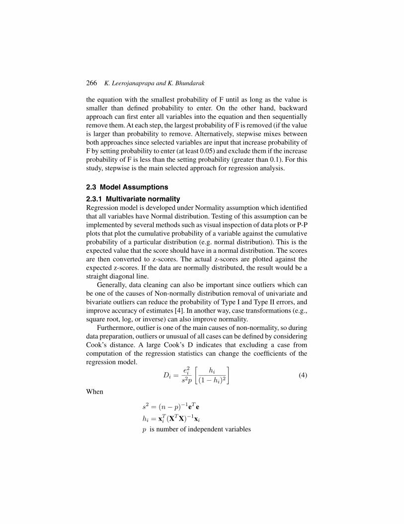
Linear regression is the most basic type of regression and commonly usedpredictive analysis as the linear equation between dependent variable (Y) andone or more independent variables (Xs).According to the record, there are 736registered companies while completed data for all defined variables from 494companies are available for analysis. The initial linear regression for Textileindustries is constructed. Table 2 shows F test inANOVAanalysis and explainsthat at least one of the defined independent variables is linearly related to theresponse variable since p-values is 0.000 which is less than the common alphalevel of 0.01. Therefore, the null hypothesis that all of the model coefficientsare 0 is rejected.

According to the results in Table 3, the result of multiple linear regressionshows influential variables of the labor demand that are Horsepower (X7),Factory area (X5), Building area (X6), Working capital (X4), and Machinery

Table 1 Characteristics of the Textile Manufacturers

Variable Mean SE Min Max

Labor demand (Y) 97.57 7.7515 5 1,422.00

Land capital (X1) 5,863.39 882.61 0 340,000.00

Building capital (X2) 9,712.28 1,476.17 0 343,925.00

Machinery capital (X3) 37,224.69 7,662.75 0 2,660,000.00

Working capital (X4) 15,849.44 5,221.21 0 2,360,000.00

Factory area (X5) 16,588.00 1,959.84 0 595,200.00

Building area (X6) 4,770.42 483.86 0 156,950.00

Horsepower (X7) 1,823.593 221.29 0 45,423.29


Table 2 Anova of the Linear Model (Textile industry)

Source SS df MS F p-value

Reg. 7,243,745.37 5 1,448,749.07 166.82 0.000*

Res. 4,238,088.32 488 8,684.61 – –

Total 11,481,833.69 493 – – –

*Significant at p-value < 0.01 level.

Table 3 Coefficients of the Linear Model (Textile industry)

Variable β SE t p-value Tolerance VIF

(Constant) 28.6246 4.6025 6.219 0.000* – –

Horsepower (X7) 0.0180 0.0013 13.509 0.000* 0.4789 2.0880

Factory area (X5) –0.0004 0.0000 –16.711 0.000* 0.4519 2.2126

Building area (X6) 0.0081 0.0005 15.286 0.000* 0.4058 2.4643

Working capital (X4) 0.0004 0.0001 4.638 0.000* 0.3104 3.2214

Machinery capital (X3) –0.0002 0.0001 –2.795 0.005* 0.2471 4.0461


capital (X3). Since coefficient p-value for all variables < 0.01, regressionequation to predict labor demand for a textile manufacturer is:

Y = 28.6246+0.0180X7 − 0.0004X5 +0.0081X6 +0.0004X4 − 0.0002X3(13)

The assumptions of regression analysis are investigated as follows. Firstly,testing multivariate normality by P-P plot (Figure 4(a)) shows that data scatterout from a straight diagonal line so multivariate normality is not assumed.Secondly, by considering the Figure 5(a); scatter plot of residuals indicateslinear relationships when they randomly spread around 0 without curvilinearpattern but without the same variance (same density both above and belowthe zero line). Therefore, assumption of a linear relationship is assumed buthomoscedasticity is not be assumed. Thirdly, the Durbin-Watson = 1.9654,which is between the two critical values of 1.5 and 2.5. Therefore, weassume that there is no first order linear auto-correlation in the multiple linearregression data. Lastly, multicollinearity is considered in Table 3. There isno VIF for individual variables which is greater than 10 or Tolerance lessthan 0.2 but VIF values of Working capital (X4) and Machinery capital (X3)are greater than 2.5. Therefore, partial correlation between two independentvariables are investigated as shown in Table 4 and found that the coefficientcorrelation of those two variables is –0.742 which is high and can be a cause of


Table 4 Coefficient Correlations of Independent Variable

(X1) (X2) (X3) (X4) (X5) (X6) (X7) (X8)

Land capital (X1) 1.000 –0.248 –0.027 0.077 –0.107 0.080 0.002 0.043

Building capital (X2) –0.248 1.000 –0.157 –0.243 0.153 –0.184 0.037 0.038

Machinery capital (X3) –0.027 –0.157 1.000 –0.742 0.252 –0.219 –0.138 –0.006

Working capital (X4) 0.077 –0.243 –0.742 1.000 –0.100 0.080 0.104 –0.017

Factory area (X5) –0.107 0.153 0.252 –0.100 1.000 –0.834 0.270 –0.063

Building area (X6) 0.080 –0.184 –0.219 0.080 –0.834 1.000 –0.562 0.059

Horsepower (X7) 0.002 0.037 –0.138 0.104 0.270 –0.562 1.000 0.038

Type (X8) 0.043 0.038 –0.006 –0.017 –0.063 0.059 0.038 1.000

multivariate. Not all assumptions are satisfied so the linear regression modelfrom the raw data should be improved by considering the suggestions givenin Sections 2.3–2.4.

Firstly, we check whether the Worker demand (Y) that is marginallynormally distributed. The histogram as show in Figure 2(a) shows that theWorker demand (Y) is non-normal distribution with a right skew. Therefore,Worker demand (Y) is transformed by log-function, log(Y) as can convergeto Normality distribution, Figure 2(b).

Since there are different types of nonlinear regression model, the relationpattern of log(Y) with other independent variables are observed. Next, therelation between log(Y) and other independent variables are shown in thescatter plot as Figure 3. The linear relation for all variables is not observedclearly. Several models either linear or nonlinear regression are explored

Figure 2 Histogram (Textile Industry).


Figure 3 Scatter plot of log (Labor demand) and other dependent variables (Textile Industry).


such as linear relation between log(Y) and independent variables by stepwiseprocedure, and different methods of independent variable transformation areexplored. Particular models are rechecked for all assumptions and then aremodified. The transforming model that satisfies all assumptions with highcorrelation coefficient is proposed as Equation (14).

By transforming Y and X7 with logarithm function, the power model(Equation (11)) is proposed as the transformation model for textile industry.Non-missing data of those two variables are obtained from 582 manufacturersin this model. The F test in the ANOVA (Table 5) shows p-values < 0.01.Furthermore, Table 6 shows the regression coefficient of log(X7) is not equalto 0 so the power model is shown in Equation (14).

log(Y) = 1.466 + 0.391 log(X7) (14)

The power model fulfils the regression assumptions since VIF is 1 (asthere is only one independent variable), testing multivariate normality by P-Pplot (Figure 4(b)) to show the relation in a straight diagonal line. In addition,scatter plot of residuals shows the residuals scatter around 0 randomly withoutpattern.

It is found that the adjusted coefficient determination (adj R2) of the linearmodel for textile manufacturer is 0.6271 with the R2 = 0.6309 which meansthat the linear regression explains 63.09% of the variance in the data. On theother hand, the adjusted R2 of power model for textile manufacturer is 0.4261with the R2 = 0.4271 which means that the power regression model explains42.71% of the variance in the Labour demand in textile industry. Generally,correlation coefficient (R) indicates the strength of the association. R values

Table 5 Anova of the Power Model (Textile Industry)


Reg. 305.633 1 305.633 432.420 0.000*

Res. 409.942 580 0.707 – –

Total 715.574 581 – – –


Table 6 Coefficients of the Power Model (Textile Industry)


(Constant) 1.466 0.111 13.195 0.000* – –

log(Horsepower) (log(X7)) 0.391 0.019 20.795 0.000* 1.000 1.000



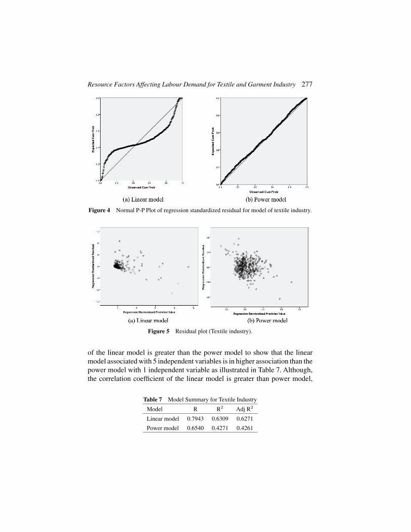
Figure 4 Normal P-P Plot of regression standardized residual for model of textile industry.

Figure 5 Residual plot (Textile industry).

of the linear model is greater than the power model to show that the linearmodel associated with 5 independent variables is in higher association than thepower model with 1 independent variable as illustrated in Table 7. Although,the correlation coefficient of the linear model is greater than power model,

Table 7 Model Summary for Textile Industry

Model R R2 Adj R2

Linear model 0.7943 0.6309 0.6271

Power model 0.6540 0.4271 0.4261


the linear model was developed from data that do not follow the modellingassumptions so those problems results in a change in the signs as well asin the magnitudes of the partial regression coefficients from one sample toanother sample. Consequently, it does not guarantee as a good labor demandforecasting model for textile industry.

5.2 Garment Manufacturers

There are 2,062 registered garment manufacturers and 656 completed datarecorded so they are employed to the analysis. Table 8 shows the mean ofworkers in particular manufacturers is 244.08 persons. The machinery capitaland working capital are as similar at 10,979,880 Baht and 10,385,550 Bahtrespectively. The mean factory area is 8,513.69 m2 and mean of building areais 2,411.27 m2. Finally, the mean operating capacity is 271.40 hp.

The F test in the ANOVA (Table 9) shows that at least one of thedefined independent variables is linearly related to the response variable (p-values < 0.001). According to the results in Table 8, the result of multiplelinear regression shows the variables that influence the labor demand ingarment manufacturer are Building capital (X2), Factory area (X5), Type (X8),

Table 8 Characteristics of the Garment Manufacturers

Variable Mean SE Min Max

Labor demand (Y) 244.08 15.80 2 4,260

Land capital (X1) 4,069.95 840.05 0 515,000

Building capital (X2) 7,958.79 735.58 0 537,000

Machinery capital (X3) 10,979.88 1,341.52 0 500,000

Working capital (X4) 10,385.55 1,343.04 0 537,000

Factory area (X5) 8,513.69 834.80 0 265,008

Building area (X6) 2,411.27 298.74 0 147,200

Horsepower (X7) 271.40 41.72 3 17,356

Table 9 Anova of the Linear Model (Garment industry)


Reg. 25,750,018.49 6 4,291,669.75 117.18 0.000*

Res. 24,245,523.98 662 36,624.66 – –

Total 49,995,542.47 668 – – –



Table 10 Coefficients of the Linear Model (Garment industry)


(Constant) 116.816 11.791 9.907 0.000* – –

Building capital (X2) 0.006 0.001 8.206 0.000* 0.683 1.465

Factory area (X5) 0.004 0.000 7.996 0.000* 0.743 1.345

Type (X8) –109.748 15.448 –7.104 0.000* 0.919 1.088

Building area (X6) 0.008 0.001 6.781 0.000* 0.870 1.149

Horsepower (X7) 0.040 0.013 2.962 0.003* 0.670 1.492

Working capital (X4) 0.001 < 0.000 2.678 0.008* 0.681 1.468


Building area (X6), Horsepower (X7), and Working capital (X4) since p-value< 0.01. As a result, regression equation to predict labor demand for a garmentmanufacturer is:

Y = 116.86 + 0.006X2 + 0.004X5 − 109.748X8 + 0.008X6

+ 0.040X7 + 0.001X4 (15)

Note: Type is dummy variable. Type = 1 if the manufacturer is small size (up to 50workers) and Type = 0 if the manufacturer is large size (greater than 50 workers).

According to the model, the coefficients indicate that every 1,000 Baht ofbuilding capital can increase worker by 0.006 person, 1,000 Baht of workingcapital can increase worker by 0.001 persons. According to the area, eachsquare meter of building area expect 0.008 worker to increase and total size ofthe factory with changes of a square meter would increase an average of 0.004person. Every additional 1 horsepower needs 0.04 workers in production.Since Type is dummy variable, the small garment manufacturer needs 109.748less than the large manufacturer as the base line.

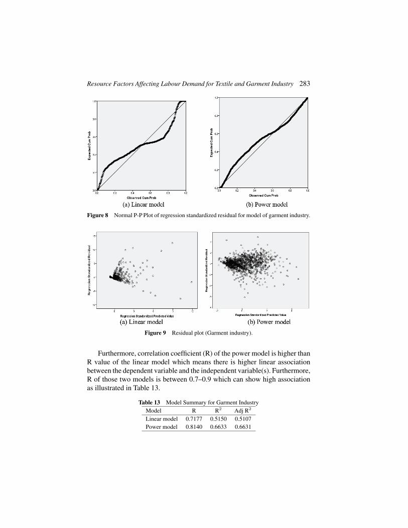
The assumptions of regression analysis are investigated as below. Firstly,testing multivariate normality by P-P plot (Figure 8(a)) shows that data scatterout from a straight diagonal line so multivariate normality is not assumed.Secondly, by considering the Figure 9(a); scatter plot of residuals indicateslinear relationships when they randomly spread around 0 without curvilinearpattern but without the same variance (same density both above and belowthe zero line). Therefore, assumption of a linear relationship is assumed buthomoscedasticity is not assumed. Thirdly, the Durbin-Watson = 1.8193, whichis between the two critical values of 1.5 and 2.5. Therefore, we assume thatthere is no first order linear auto-correlation in the multiple linear regression


data. Lastly, multicollinearity is considered in Table 12 and there is no VIFfor individual variables which are greater than 10 or greater than 2.5 or withTolerance less than 0.2 so that there is no multicollinearity for all definedindependent variables in the defined model. Not all assumptions are passed,so we can improve the model with methods for variable transformation.

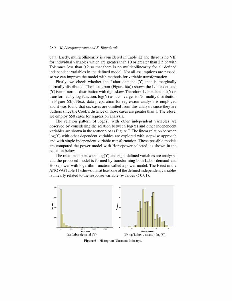
Firstly, we check whether the Labor demand (Y) that is marginallynormally distributed. The histogram (Figure 6(a)) shows the Labor demand(Y) is non-normal distribution with right skew. Therefore, Labor demand (Y) istransformed by log-function, log(Y) as it converges to Normality distributionin Figure 6(b). Next, data preparation for regression analysis is employedand it was found that six cases are omitted from this analysis since they areoutliers since the Cook’s distance of those cases are greater than 1. Therefore,we employ 650 cases for regression analysis.

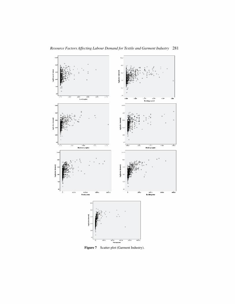
The relation pattern of log(Y) with other independent variables areobserved by considering the relation between log(Y) and other independentvariables are shown in the scatter plot as Figure 7. The linear relation betweenlog(Y) with other dependent variables are explored with stepwise approachand with single independent variable transformation. Those possible modelsare compared the power model with Horsepower selected, as shown in theequation below.

The relationship between log(Y) and eight defined variables are analysedand the proposed model is formed by transforming both Labor demand andHorsepower with logarithm function called a power model. The F test in theANOVA(Table 11) shows that at least one of the defined independent variablesis linearly related to the response variable (p-values < 0.01).

Figure 6 Histogram (Garment Industry).


Figure 7 Scatter plot (Garment Industry).


Table 11 Anova of the Power Model (Garment industry)


Reg. 1202.837 1 1202.837 3196.772 0.000*

Res. 610.680 1623 0.376 – –

Total 1813.517 1624 – – –


Table 12 Coefficients of the Power Model (Garment industry)


(Constant) 1.968 .044 45.016 0.000*

log(Horsepower) (log(X7)) 0.636 .011 56.540 0.000* 1.000 1.000


According to the results in Table 12, the variables that influence the labordemand with logarithm transformation in garment manufacturer are logarithmof horsepower, since p-value < 0.01. The regression equation shows relationequation to predict the labor demand that transform to log(Y) from the onlyone variable for a garment manufacturer in Equation (16).

log(Y) = 1.968 + 0.636 log(X7) (16)

The appropriate of proposed regression model is confirmed by the results ofassumption verification. Firstly, Figure 8(b) shows the distribution of residualof the model is normality as the expected cumulative probability of log(y)distributes along the straight diagonal line so the normality distribution isassumed. Secondly, residual plot in Figure 9(b) indicates linear relationshipswhich assumed as residuals randomly spread around 0 without curvilinearpattern. Thirdly, the density of both above and below the zero line is equivalent.Therefore, assumption of homoscedasticity is assumed. Fourthly, the Durbin-Watson = 1.6649, therefore there is no first order linear auto-correlation in themultiple linear regression data. Lastly, multicollinearity test can be acceptedsince there is only one independent variable in this model.

It is found that the adjusted coefficient determination (adj R2) of the linearmodel for garment manufacturer is 0.5107 with the R2 = 0.5150, which meansthat the linear regression explains 51.50% of the variance in the data. Onthe other hand, adj R2 of the power model is 0.6631 with the R² = 0.6633,which means that the power model explains 66.33% of the labor demandin textile industry. It is also found that adj R2 of the power model withone independent variable is higher than adj R2 of the linear model with sixindependent variables.


Figure 8 Normal P-P Plot of regression standardized residual for model of garment industry.

Figure 9 Residual plot (Garment industry).

Furthermore, correlation coefficient (R) of the power model is higher thanR value of the linear model which means there is higher linear associationbetween the dependent variable and the independent variable(s). Furthermore,R of those two models is between 0.7–0.9 which can show high associationas illustrated in Table 13.

Table 13 Model Summary for Garment IndustryModel R R2 Adj R2

Linear model 0.7177 0.5150 0.5107Power model 0.8140 0.6633 0.6631


6 Conclusion and Further Studies

There are two objectives for this article. The first objective is to define thecorrelation between particular resource variables with the labour demandwhich can be explained by the linear model for both industries. Thesecond objective is to define the suitable forecasting model to predictlabour demands by proposing the model which satisfied all modellingassumptions.

According to the multiple linear models for textile and garment industries(Equation (13) and Equation (15)), it is found that textile and garmentmanufacturers are different in nature although they are in the same supplychain. The textile sector relies on technology and machinery so the textilefiber manufacturers invested a lot of money in machinery (high mean valueof Machinery capital). As a result, the new technologies invested can reducenumber of workers in their process but they may need high skilled workersto be able to implement the technology. On the hand, the garment sectorremains one of the most labor intensive industries and they are different insize of manufacturers. They need a lot of workers in manufacturing processe.g. sawing or cutting so mean of number of workers is higher than textilefiber manufacturer.

However; those linear models could not meet the associated assumptionsby linear relationship and homoscedasticity. This study also improves theliner model by using transformations to achieve all regression assumptionsin order to fulfil the second objectives. The power model constructs therelationship between log(Labour demand) and log(Horsepower) which canreduce the complexity of using multivariate predictors in order to ensure thatthe model can be a suitable forecasting model under the defined modellingassumptions. The power model proposed for garment industry (Equation (14))can show the better forecasting model than the power model for textile industry(Equation (16)) as shown by the higher number of correlation coefficient (R)and a multiple correlation coefficient (R2).

This article proposes the basic forecasting model for cross-sectional dataparticularly textile and garment companies in Thailand which can be used asthe initial guideline for workforce planning. For further improvements, morerelevant variables to the labor demand should be defined since the limitednumbers of variables are available in this record as the secondary data. Inaddition, time series data should be brought to the further studies.


References

[1] Bureau of Labor Statistics. (2015). Projections of the Labor Force, 2014–24.Available at: http://www.bls.gov/careeroutlook/2015/article/projections-laborforce.htm [Accessed: 16-Feb-2016].

[2] Samuelson, P. A. and Nordhaus, W. D. (2005). Macroeco-nomics, 18th Edn. Boston, MA: McGraw-Hill/Irwin. Available at:http://trove.nla.gov.au/version/13058406

[3] The Office of Industrial Economics. (2016). Industrial Economic Con-ditions in 2016 and Outlook for 2017.

[4] Osborne, J. W., Christensen, W. R., and Gunter, J. (2001). EducationalPsychology from a Statistician’s Perspective: A Review of the Power andGoodness of Educational Psychology Research. In National Meeting ofthe American Education Research Association (AERA), Seattle, WA.

[5] Region Government of the Hong Kong Administrative. (2012). Reporton Manpower Projection to 2018.

[6] Nadvi, K., Thoburn, J. T., Thang, B. T., Ha, N. T. T., Hoa, N. T.,Le, D. H., and Armas, E. B. D. (2004). Vietnam in the global garmentand textile value chain: impacts on firms and workers. J. Int. Dev., 16,111–123.

[7] Taplin, Ian M., Jonathan Winterton, and Ruth Winterton. (2003) “Under-standing labour turnover in a labour intensive industry: evidence fromthe British clothing industry.” J. Manage. Stud. 40, 1021–1046.

[8] Dong, J., Ren, C., Ren, S., Shao, B., Wang, Q., Wang, W., and Ding, H.(2008). iRDM: A solution for workforce supply chain management inan outsourcing environment. In Service Operations and Logistics, andInformatics, IEEE/SOLI 2008. IEEE International Conference, Vol. 2,2496–2501.

[9] Scheffler, R. M., Liu, J. X., Kinfu, Y., and Dal Poz, M. R. (2008). Fore-casting the global shortage of physicians: an economic-and needs-basedapproach. Bull. World Health Organ. 86, 516–523.

[10] Liu, J., Love, P. E., Sing, M. C., Carey, B., and Matthews, J. (2015).Modeling Australia’s construction workforce demand: Empirical studywith a global economic perspective. J. Constr. Eng. Manag. 141,p. 5014019.


[11] Wong, J. M., Chan, A. P., and Chiang, Y. H. (2011). Constructionmanpower demand forecasting: A comparative study of univariate timeseries, multiple regression and econometric modelling techniques. Eng.Constr. Archit. Manag. 18, 7–29.

[12] Wong, J. M., Chan, A. P., and Chiang, Y. H. (2005). Time series forecastsof the construction labour market in Hong Kong: the Box-Jenkinsapproach. Constr. Manage. Econ. 23, 979–991.

[13] U. S. B. of L. Statistics. (1929). Handbook of labor statistics, U.S. G.P.O.

Biographies

Kanogkan Leerojanaprapa went to the Thammasat University, where shestudied Applied Statistics and obtained her degree in 1999. She continued tostudy Master degree in Statistics in Chulalongkorn University and obtainedher degree in 2002. She worked for four years for King Mongkut’s Institute ofTechnology Ladkrabang (KMITL). She holds a PhD in Management sciencesince 2014 from University of Strathclyde, UK. After her graduation, shereturned to KMITL where she is now a lecturer in Statistics department. Herresearch focus in the area of risk analysis, Bayesian network, and applicationsof statistical models. She has published articles in various peer reviewedinternational journals and conferences.


Komn Bhundarak obtained a B.BA. in Industrial Management from Facultyof Accountancy and Commerce, Thammasat University, in 1985. He workedfor 3M Thailand more than 10 years while pursuited MBA from ThammasatUniversity in 1989 and Master of Science in Infornation Technology fromKasetsart University in 2001. Then he became a lecturer in 2009 and earnedhis Doctoral in Business with Management since 2014 from University ofPlymouth, UK. After his graduation, he joined Thammasat Business School,Thammasat University, where he is now a Department Head, OperationsManagement Department. His research focus in the area of supply chainmanagement and business analytics.

Date post:	06-Sep-2018
Category:	Documents
Upload:	nguyenthuy
View:	230 times
Download:	0 times

Resource Factors Affecting Labour Demand forTextile … Resource Factors Affecting Labour Demand...

Documents