Resource Investment Optimization System...

NATURAL CAPITAL PROJECT

Resource Investment Optimization System (RIOS)

v1.1.0

Introduction & Theoretical Documentation

Step-by-Step User’s Guide

1 Natural Capital Project, Stanford University

2 The Nature Conservancy

3 Fauna & Flora International

Resource Investment Optimization System

Introduction & Theoretical Documentation

May 2015

Contributing Authors: Adrian Vogl1, Heather Tallis2, James Douglass1, Rich

Sharp1, Stacie Wolny1, Fernando Veiga2, Silvia Benitez2, Jorge León2, Eddie

Game2, Paulo Petry2, João Guimerães3, Juan Sebastián Lozano2

Natural Capital Project, 2Latin America Water Funds Platform, 3TNC Northern

PLEASE NOTE:

05 May 2015

This version of the RIOS User Guide supersedes the previous version, released in January 2015.

Several changes have been made to RIOS since the previous User Guide. These changes

include:

1) The Portfolio Translator module of RIOS has been improved and added back to the RIOS

toolset. This module can be used to turn RIOS activity portfolio outputs into inputs for

InVEST SDR and Water Yield models.

2) It is no longer required to map land use/land cover classes to ‘general’ LULC types in the

LULC Classification Table. Instead, users provide an LULC Biophysical Coefficients

table, which contains much of the same coefficient information as the previous

general_lulc_coefficients.csv (but without the ‘general_lulc’ mapping), and including

fields related to InVEST SDR and Water Yield models. As in previous versions of RIOS,

default values for these coefficients are provided to get users started with average data, in

the table RIOS_default_coefficients.csv. 3) The clumping function for activities has been disabled, due to unexpected behavior near

stream channels that caused activities to be preferentially chosen away from streams.

This function is being further developed and we expect to re-introduce it in a future

release.

Table of Contents

I. Introduction: The RIOS Development Process ......................... 1

II. Overview of RIOS Workflow ...................................................... 2

i. RIOS Investment Portfolio Advisor ................................................................ 3

Objectives

Transitions and Activities

Diagnostic Screening

Additional Portfolio Options

Budget Allocation

Select Activity Portfolio

Interpreting the Portfolio

ii. RIOS Portfolio Translator .............................................................................. 20

iii. Estimating benefits of RIOS portfolios ......................................................... 24

III. Model Descriptions ..................................................................... 27

i. Erosion Control for Drinking Water Quality and Reservoir Maintenance .... 27

ii. Nutrient Retention: Phosphorus ..................................................................... 32

iii. Nutrient Retention: Nitrogen ........................................................................ 36

iv. Flood Mitigation ............................................................................................ 41

v. Groundwater Recharge Enhancement ........................................................... 45

vi. Dry Season Baseflow ..................................................................................... 51

vii. Biodiversity .................................................................................................... 56

viii. Other Objectives ............................................................................................ 56

IV. Data Requirements ..................................................................... 57

i. General Data Requirements ........................................................................... 57

ii. Required Data Pre-Processing ....................................................................... 72

iii. Default LULC Data Provided with RIOS ...................................................... 72

1

I. Introduction

The Resource Investment Optimization System (RIOS) was developed by the Natural

Capital Project (NatCap), in close collaboration with The Nature Conservancy (TNC)

and the Latin America Water Funds Platform (a partnership among The Nature

Conservancy, the Inter-American Development Bank, GEF, and FEMSA). RIOS is a

software tool for prioritizing investments in ecosystem services that can help to answer a

critical question facing decision makers who wish to invest in ecosystem services with

limited resources:

Which set of investments (in which activities, and where) will yield the greatest

returns toward multiple objectives?

RIOS introduces a science-based approach to prioritizing watershed investments by

identifying where protection or restoration activities are likely to yield the greatest

benefits for both people and nature at the lowest cost. RIOS can facilitate the design of

investments for a single management goal or several at once, including erosion control,

water quality improvement (for nitrogen and phosphorus), flood regulation, groundwater

recharge, dry season water supply, and terrestrial and freshwater biodiversity. RIOS can

also incorporate other goals into the portfolio design such as avoiding high opportunity

cost areas such as production agriculture, or directing investments in a way that benefits

poor populations. When RIOS is used in a process of stakeholder engagement,

investment design, and impact modeling, investors can also address other critical

questions such as:

What change in ecosystem services can I expect from these investments?

How do the benefits of these investments compare to what would have been

achieved under an alternate investment strategy (i.e. what is the benefit of

science in guiding my investments)?

RIOS is a practical tool that operates independently of scale or location (within the

constraints of available data), meaning that it can be used to inform a broad selection of

prioritization issues at the continental, country, or county scale. Using widely available

data on land use and management, climate, soils, topography, and service demands, it

will also be able to direct investments and estimate returns in any region at varying

scales.

A tool with this flexibility and generality is the result of extensive development, drawing

input from broad expertise and testing in a diverse set of operational water funds.

2

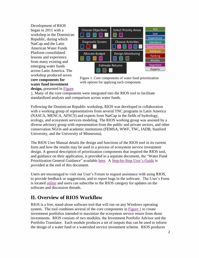
Development of RIOS

began in 2011 with a

workshop in the Dominican

Republic, during which

NatCap and the Latin

American Water Funds

Platform consolidated

lessons and experience

from many existing and

emerging water funds

across Latin America. The

workshop produced seven

core components for

water fund investment

design, presented in Figure

1. Many of the core components were integrated into the RIOS tool to facilitate

standardized analysis and comparison across water funds.

Following the Dominican Republic workshop, RIOS was developed in collaboration

with a working group of representatives from several TNC programs in Latin America

(NASCA, MENCA, AFSCS) and experts from NatCap in the fields of hydrology,

ecology, and ecosystem services modeling. The RIOS working group was assisted by a

diverse advisory group with representation from the public and private sectors, and other

conservation NGOs and academic institutions (FEMSA, WWF, TNC, IADB, Stanford

University, and the University of Minnesota).

The RIOS User Manual details the design and functions of the RIOS tool in its current

form and how the results may be used in a process of ecosystem service investment

design. A general description of prioritization components that inspired the RIOS tool,

and guidance on their application, is provided in a separate document, the “Water Fund

Prioritization General Guidance” available here. A Step-by-Step User’s Guide is

provided at the end of this document.

Users are encouraged to visit our User’s Forum to request assistance with using RIOS,

to provide feedback or suggestions, and to report bugs in the software. The User’s Form

is located online and users can subscribe to the RIOS category for updates on the

software and discussion threads.

II. Overview of RIOS Workflow

RIOS is a free, stand-alone software tool that will run on any Windows operating

system. The tool combines several of the core components in Figure 1 to create

investment portfolios intended to maximize the ecosystem service return from those

investments. RIOS consists of two modules: the Investment Portfolio Advisor and the

Portfolio Translator. Each module produces a set of outputs that can be used to inform

the design of a water fund or a watershed service investment scheme. RIOS produces

Figure 1. Core components of water fund prioritization

with options for applying each component.

http://www.naturalcapitalproject.org/pubs/Water_Fund_Prioritization_Guidance_Document.pdf

http://forum.naturalcapitalproject.org/

3

two major outputs: an investment portfolio (used to guide where, and in what activities,

investments can be made) and a set of land use scenarios that represent the portfolio

implemented on the current landscape (which can then be used to model the change in

services resulting from the portfolio). In addition, RIOS produces several intermediate

output score maps that help users to interpret the results and to understand why some

areas are selected for certain activities over others.

First, the Investment Portfolio Advisor module uses biophysical and social data,

budget information, and implementation costs to produce ‘investment portfolios’ for a

given water fund area. These portfolios integrate the Diagnostic Screening and Select

Priority Areas key components of water fund investment prioritization (Figure 1; see

Water Fund Prioritization General Guidance Document for a description of all key

components). The investment portfolio shows what is likely to be the most efficient and

effective set of investments the fund can make, given a specific budget. The portfolio is

a map of activities (e.g. protection, restoration, reforestation, improved agricultural

practices), indicating where investments in each activity will give the best returns across

all water fund objectives. Most water funds have more than one objective. RIOS is

designed to address multiple ecosystem service objectives (e.g. erosion control, water

quality regulation, seasonal flow & flood regulation), and can also be used to address

biodiversity or other conservation or social objectives (e.g. poverty alleviation,

alternative livelihoods) through user-defined inputs.

Once the investment portfolio is created, the Portfolio Translator module guides the

user through a set of options to generate scenarios that reflect the future condition of the

watershed if the portfolio is implemented. The scenarios generated by the Portfolio

Translator module are designed to be used as inputs to the InVEST suite of tools

(http://naturalcapitalproject.org/InVEST.html) for estimating the ecosystem service

return on investment from each portfolio. RIOS creates all required input files for the

InVEST sediment retention and water yield/water purification models. Users can also

choose to use these scenarios with any ecosystem service model to estimate benefits –

although keep in mind that additional data and pre-processing steps may be required.

With InVEST, users can also compare the improvements in ecosystem services to

returns from RIOS with those achieved from other scenarios of investments, such as an

ad-hoc investment approach (requires additional user input). This gives users a sense of

how much the scientific approach employed in RIOS improves investment returns.

i. RIOS Investment Portfolio Advisor

The RIOS Investment Portfolio Advisor module combines several of the core

components, biophysical data, and information on activities and their associated costs to

develop investment portfolios. We attempted to incorporate as many of the options for

each of the core components as possible to allow maximum flexibility of the tool. RIOS

inputs relate to a series of questions that help users to step through these components, as

presented in Figure 2 and in the text that follows.

http://www.naturalcapitalproject.org/pubs/Water_Fund_Prioritization_Guidance_Document.pdf

http://naturalcapitalproject.org/InVEST.html

4

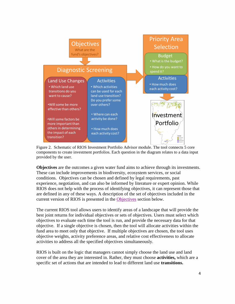
Figure 2. Schematic of RIOS Investment Portfolio Advisor module. The tool connects 5 core

components to create investment portfolios. Each question in the diagram relates to a data input

provided by the user.

Objectives are the outcomes a given water fund aims to achieve through its investments.

These can include improvements in biodiversity, ecosystem services, or social

conditions. Objectives can be chosen and defined by legal requirements, past

experience, negotiation, and can also be informed by literature or expert opinion. While

RIOS does not help with the process of identifying objectives, it can represent those that

are defined in any of these ways. A description of the set of objectives included in the

current version of RIOS is presented in the Objectives section below.

The current RIOS tool allows users to identify areas of a landscape that will provide the

best joint returns for individual objectives or sets of objectives. Users must select which

objectives to evaluate each time the tool is run, and provide the necessary data for that

objective. If a single objective is chosen, then the tool will allocate activities within the

fund area to meet only that objective. If multiple objectives are chosen, the tool uses

objective weights, activity preference areas, and relative cost effectiveness to allocate

activities to address all the specified objectives simultaneously.

RIOS is built on the logic that managers cannot simply choose the land use and land

cover of the area they are interested in. Rather, they must choose activities, which are a

specific set of actions that are intended to lead to different land use transitions.

5

Transitions represent the types of land management changes that managers would

actually like to create on the ground in order to achieve their objectives. For more

information about transitions, see the Transitions and Activities section below.

More specifically, activities are the specific set of actions in which a water fund can

invest, with the goal of achieving the required land management transitions. These can

be chosen through expert consultation, direct experience, or they may be based on the

results of field experiments or pilot studies that inform which activities are likely to be

most effective for a fund. RIOS does not assist in selecting which activities should be

considered by a fund, but once activities are selected and associated with one of the

transition types built into RIOS, it can identify where each activity is likely to give the

greatest returns towards the full set of the water fund’s objectives. For more information

about the relationship between activities and transitions, see the Transitions and

Activities section below.

Budget allocation can be focused on achieving the best return on investment (ROI),

targeting funds based on some attribute of the system (e.g. proportional distribution of

funds based on watershed area or density of beneficiaries), targeting based on previous

experience, or through negotiation. The default budget allocation approach in RIOS is

driven by cost effectiveness, but users can override this to pre-allocate funds among

activities or allocate the budget based on some other attribute. Details of these methods

are given in the Budget Allocation section below.

Diagnostic screening gives a view of where water fund investments are likely to be most

effective across the landscape. Screening can be done using quantitative models, ranking

methods or expert opinion. The potential for using quantitative models with dynamic

landscape optimization is being investigated for future releases of RIOS, but the tool

currently relies on ranking models for diagnostic screening and incrementally chooses

areas with the highest ROI. Some elements of model structure are informed by expert

opinion. This process is described in the Diagnostic Screening section below.

Once activities are chosen, budgets are allocated, and a diagnostic screening has been

performed, RIOS identifies where on the landscape investments are likely to produce the

greatest returns for a given budget (i.e. are most cost effective). In practice, the selection

of priority areas can be done using cost effectiveness or through negotiation among

stakeholders involved in planning the fund. RIOS uses the cost effectiveness approach,

selecting the areas with the highest rank per monetary unit until the defined budget is

spent. Together, these selected areas form the investment portfolio.

Objectives

The following objectives are included in RIOS.

Erosion control for drinking water quality

Investment in watersheds can help prevent excessive soil erosion, improve

downstream water quality and potentially decrease drinking water treatment costs and

6

negative health impacts. This objective relates to regulation of sheetwash, rill and

gully and bank erosion. RIOS cannot suggest or prioritize activities that regulate in-

channel erosion or deposition, as these dynamics are not accounted for in the

underlying models. This objective is identical to “Erosion control for reservoir

maintenance” (below). The distinction is included here because an earlier version of

the InVEST sediment model provided for valuation of sediment retention based on

either drinking water quality or avoided reservoir dredging. The current sediment

model (SDR) does not provide this valuation, but the user may still wish to make this

distinction, providing different inputs for each type of sediment objective.

Erosion control for reservoir maintenance

Erosion control that keeps sediment out of waterways can also prevent its deposition in

reservoirs, where it can reduce the production capacity of hydropower facilities or

damage irrigation reservoirs and infrastructure (turbines, pumps, etc), shorten the

lifetime of the reservoir or increase sediment management costs (such as dredging).

This objective also relates to regulation of sheetwash, rill and gully and bank erosion

control, but cannot suggest or prioritize activities that regulate in-channel erosion or

deposition. This objective is identical to “Erosion control for drinking water quality”

(above). The distinction is included here because an earlier version of the InVEST

sediment model provided for valuation of sediment retention based on either drinking

water quality or avoided reservoir dredging. The current sediment model (SDR) does

not provide this valuation, but the user may still wish to make this distinction,

providing different inputs for each type of sediment objective.

Nutrient retention (Nitrogen)

A watershed’s ability to prevent the export of nitrogen from upstream sources can

improve downstream water quality, and potentially decrease drinking water treatment

costs and nitrogen-related health risks. This objective relates to regulation of any form

of nitrogen, but does not capture regulation of any other pollutant (e.g. phosphorus,

bacteria, pesticides, heavy metals).

Nutrient retention (Phosphorus)

A watershed’s retention of phosphorus from upstream sources can improve

downstream water quality, aquatic habitat and biodiversity, and potentially decrease

drinking water treatment costs and phosphorus-related health risks. This objective

relates to regulation of any form of phosphorus, but does not capture regulation of any

other pollutant (e.g. nitrogen, bacteria, pesticides, heavy metals).

Flood mitigation Investment in watersheds can help to intercept rainfall, slow overland flow of water,

and increase travel time of water to the river, decreasing the peak magnitude of floods.

Reducing the size of peak flood flows can mitigate impact to infrastructure and private

property and reduce the risk to human life. In reality, natural capital investment can

only significantly influence flood peak flows in average to medium-sized storms such

as 10 year return period events or smaller. For very large storms (i.e. 100 year return

7

period events), flood risk is more dependent on geography and characteristics of the

channel network than by water fund investments. This objective represents the role

that natural capital can play in retaining water on the landscape and reducing flood

peaks; however the impact of activities will diminish as the storm size increases.

Groundwater Recharge Enhancement Investment in watersheds can help to intercept rainfall, slow overland flow of water,

and increase the potential for water to percolate past the soil surface and recharge

underlying aquifers. In areas that depend heavily on groundwater for their water

supply, enhancing groundwater recharge can help to maintain water table levels,

enhancing water security and decreasing the costs of extraction. This objective

represents the role that natural capital can play in capturing water and facilitating its

movement into subsurface aquifers. In its current release, RIOS can identify activities

that will promote groundwater recharge enhancement in unconfined aquifers, and is

particularly applicable in areas where major recharge features have been mapped (such

as karst areas).

Dry Season Baseflow

Vegetation can intercept rainfall, slow overland flow of water, and increase temporary

storage of subsurface water in soils, floodplains, and streambanks, which is later

released slowly during the dry season to increase the magnitude and permanence of

low flows. This objective represents the role that natural capital can play in capturing

and storing water and facilitating its slow release into streams.

Biodiversity Biodiversity, the natural variation in life forms, is intimately linked to the production

of environmental services. Patterns in biodiversity are inherently spatial, and can be

estimated by analyzing maps of land use and land cover in conjunction with threats.

RIOS does not model biodiversity directly, but users may apply outputs from other

models or draw from expert local knowledge to specify biodiversity scores as an input

and to choose how areas meeting these objectives will be ranked relative to the rest of

the objectives chosen.

Other

Users may have results from other models or prioritization areas that they wish to

consider when developing investment portfolios. RIOS allows users to enter score

maps for up to three “other” objectives, and to choose how areas meeting these

objectives will be ranked relative to the rest of their objectives. These “other”

objectives work in the same way as the Biodiversity objective, and are included so that

users can incorporate other models or data sources to address additional user-defined

goals.

8

Transitions and Activities

At its core, watershed service investment

aims to change the way watersheds are

managed to ensure that objectives are met

in the future. Managers have a range of

activities they can invest in to realize their

desired changes, such as the

implementation of fencing, silvopastoral

systems, terracing and so on. But these

changes are often not the desired endpoint

of the investment. Water funds may invest

in these activities because they cause a

desirable initial transition in the vegetation

or management practices that will

ultimately impact the fund's future

objectives. Water funds have a diverse set

of activities they can choose from to cause

a relatively finite set of changes on the

landscape (See Figure 3). Each transition

has some potential to affect many of the processes that regulate hydrologic processes

and biodiversity. These include the maintenance of habitat quality and feeding and

breeding resources for species as well as water infiltration rates, soil storage capacity,

vegetation cover and structure, extent of the rooting zone, nutrient uptake rates, overland

flow rates, and rainfall interception.

As suggested in Figure 3, there are several activities that can cause the same kinds of

desirable changes but at different costs and in different parts of the landscape.

Given this variation, RIOS separates transitions and activities and uses information

about each in the diagnostic screening and portfolio selection process. Landscape

changes (Transitions) are fixed within the software, while Activities are defined by the

user in the Land Use Classification input table. The transitions included in the current

RIOS tool are:

o Keep native vegetation (protection)

o Revegetation (unassisted)

o Revegetation (assisted)

o Agricultural vegetation management

o Ditching

o Fertilizer management

o Pasture management

Below we give a brief description of each transition that is used in RIOS, and give some

specific examples of some types of activities that users might use to achieve each of the

transitions. Activities in RIOS are entirely user-defined, so the examples of activities

that might achieve each transition given here are not intended to be inclusive of all

potential activities in which watershed investors might decide to invest.

Figure 3. Relationship between water fund

investments in activities and desired

transitions in targeted watersheds.

9

Keep native vegetation: A transition that focuses on retaining native vegetation

that would likely be lost otherwise (i.e. protecting existing habitat). This is only

possible in parts of the watershed that currently have native vegetation.

Maintenance of existing native vegetation can be achieved by educating local

people about the benefits of conservation and changing their mindset about land

management practices. It can also be achieved by fencing off areas of native

vegetation to reduce the likelihood of livestock entering and disturbing it and to

discourage people from entering and harvesting natural products, hunting, or

converting the area for other uses. If native vegetation exists within a protected area

that is not well enforced, improving protected area management (establishing a new

protected area, improving management of existing protected areas, hiring park

guards, adding fencing, providing education or creating incentives for surrounding

communities to respect boundaries,) can help keep native vegetation in place.

Revegetation (unassisted): This transition refers to the revitalization of vegetation

on degraded or bare lands without active interventions. This can include providing

space for the regrowth of native or non-native species and can apply to any type of

system (e.g. grassland, forest, wetland). Examples of activities that might be

associated with this transition are education, which can inform locals about the

benefits of revegetation and encourage them to promote the process to occur,

fencing, and livestock exclusion, which will help prevent further degradation from

occurring and allow vegetation to recover in protected areas.

Revegetation (assisted): This transition represents revitalization of vegetation on

degraded or bare lands through active interventions. Education can encourage

private landowners to make their own investments in revegetation. Tree planting is

a specific activity that is common in some watershed areas that may relate to native

or non-native tree planting into degraded forest, pastures, or degraded agricultural

lands. Native vegetation planting refers to the planting of any other vegetation

including grasses, herbaceous plants, shrubs, wetland plants, or riparian vegetation

and can include activities to maintain that vegetation such as irrigation, weeding,

thinning, replanting, and invasive species control. Finally, some kinds of

silvopastoral practices can encourage revegetation through improved management

of pastures or rangelands. These can include planting of trees in pastures, fencing or

otherwise keeping cattle out of riparian areas or other natural vegetation.

Agricultural vegetation management: This transition represents increases in crop

structure, coverage and/or diversity. It can be motivated by crop planting practices

that increase or diversify crop cover, such as planting cover crops, changing crop

rotation patterns or practices, increasing crop diversity, or promoting agroforestry

practices. This activity may also include any direct incentives given to landowners

or managers to change their cropping practices. Education can also be employed to

inform farmers of options in vegetation management.

10

Ditching: This transition refers to activities that act to improve infiltration of water

and slow the transport of sediment and nutrients on agricultural or degraded lands.

This transition can be achieved for example by the use of contour ditching, which

acts to stop water from running down agricultural slopes and causing erosion. Water

stays in the ditch and gradually sinks into the soil. More generally, activities like

terracing (with or without associated ditching) can also be associated with this

transition. Education can be useful here as well to introduce land managers to the

ideas and approaches for modifying the landscape and their associated benefits.

Ditching to channel flow to drain excess water more quickly off of agricultural

lands is not included in this transition.

Fertilizer management: This transition is related to any activity that changes the

way fertilizer is applied to crops or pastures. It reflects changes in management

practices that aim to supply crops with adequate nutrients to achieve optimal yields,

while minimizing nonpoint source pollution and contamination of groundwater, and

maintaining and/or improving the condition of soil. Examples of such practices

include altering the rate and method of application to match soil type and crop

needs, and changing irrigation amount and timing to minimize excess nutrient

runoff.

Pasture management: This transition reflects changes in management practices on

pastures or natural rangelands, such as a change from using the entire pasture area

continuously to splitting area into smaller paddocks and intensively grazing each

paddock for a short period of time. Livestock management represents a set of

activities that can include fencing, training, reducing stocking densities, and altering

pasture rotation practices. Some kinds of silvopastoral practices can also be

considered pasture management, those that encourage improved management of

pastures or rangelands such as decreasing stocking densities, or providing direct

incentives to landowners to change their pasture and rangeland management

behavior.

RIOS users provide data on which transitions they would like to achieve, and whether

they expect some transitions to be more effective at providing improvements towards

each objective. Users also provide data on which activities the fund can invest in and

identify which kinds of transitions each can cause (currently, activities are assumed to be

equally effective in bringing about a transition, though it is possible to work around this

assumption, and future versions of RIOS may allow for varying this). In addition, users

provide data on which activities can be implemented on which land use/land cover

types. See Additional Portfolio Options section below for more details on weighting

transitions, and Table IV.3 for information on assigning activities to land use/land cover

types.

11

Diagnostic Screening

The primary function of the RIOS tool is to enable an initial diagnostic assessment of

areas and activities where investments will have the greatest impact on ecosystem

services. The point of a diagnostic screening process is to estimate how the potential for

watershed investment impact varies across the focal region. The screening gives a view

of the whole landscape and allows investors to see the entire picture before focusing in

on priority areas defined by a set budget. There are many approaches that can be used

for diagnostic screening and they vary tremendously in sophistication, data, capacity and

resource requirements and complexity. The RIOS tool strikes a balance between

complexity and practicality with its current approach.

The underlying premise of the RIOS diagnostic screening approach is that a small set of

biophysical and ecological factors determine the effectiveness of each transition in

accomplishing each chosen objective. We define a set of critical factors for each

objective through careful literature review. From a review of experimental studies,

review papers, and hydrologic model documentation, we identified the subset of

landscape factors that were most frequently identified as being important for

determining the magnitude of the source (of sediment, pollutants, or flow that would be

mitigated by activities) and the effectiveness of activities that impact each of the

potential objectives (erosion control, nutrient retention, flood mitigation, etc).

Because budget allocation and fund investments are annual or multi-year processes, the

RIOS tool focuses on impacts of transitions on an annual or longer-term time scales.

Therefore, factors identified from the literature review as influencing impacts on a daily

or seasonal basis are not included in the software’s framework (such as antecedent soil

moisture, daily rainfall intensity). The one exception is the Flood Mitigation Impact

Ranking Model, which measures impact from episodic storm events and therefore

includes factors influencing ecosystem service provision on a daily or seasonal basis

(such as rainfall intensity).

A different set of factors is identified as most critical for influencing impacts on each

separate objective. Much of the impact of transitions will be determined by conditions

on the surrounding landscape. Therefore, RIOS relies on a set of four major components

across its framework that captures the processes influencing these impacts and the

effectiveness of activities (1) upslope source magnitude (2) on-pixel source (3) on-pixel

retention (4) downslope retention. Each of the aforementioned components is

represented by one or more factors within each objective. Details on the factors selected

by objective are described further below in Section III – Model Descriptions.

The diagnostic screening process allows users to survey a region for areas that pose the

highest risk of damaging or improving delivery of ecosystem services. Locations are

ranked based on a set of biophysical factors indicating how effective different kinds of

protective, restorative, or management transitions are likely to be. These factors are

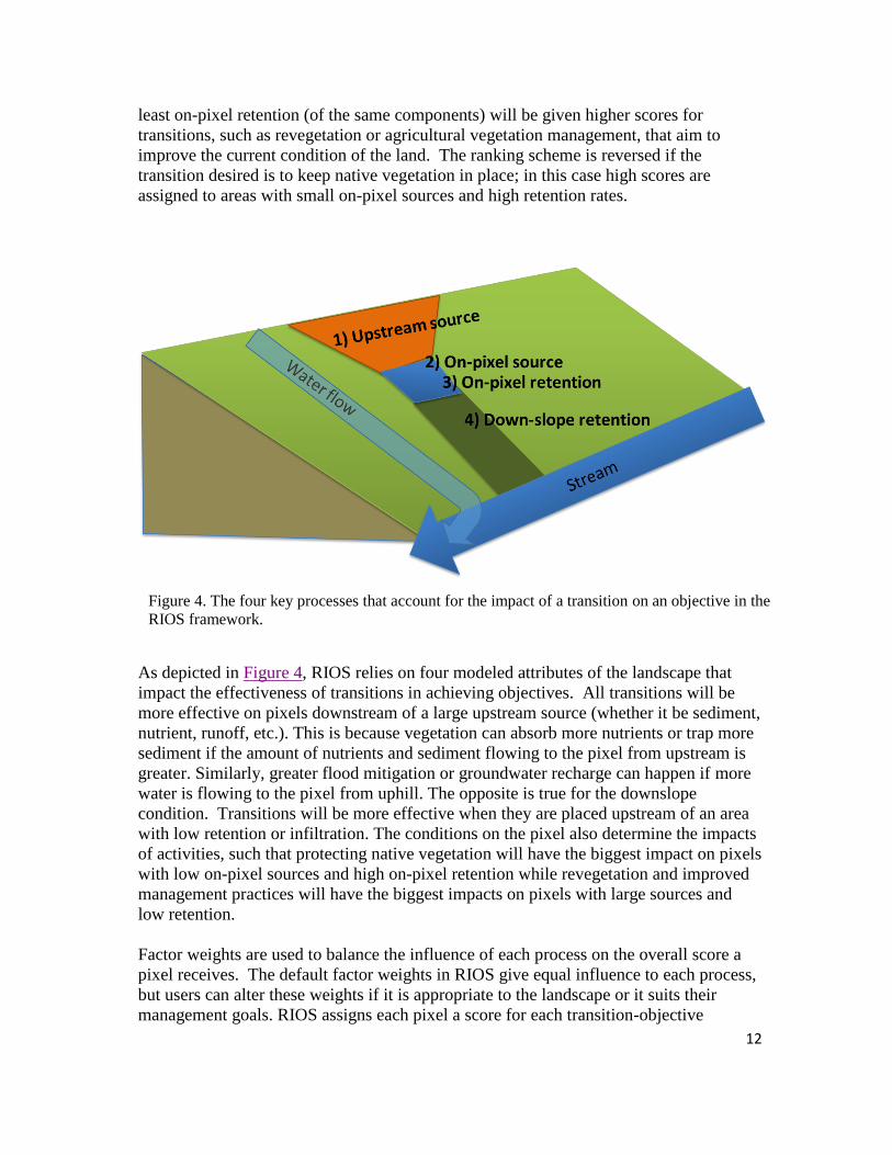
based both on the local conditions and the landscape context, as indicated in Figure 4.

Areas with the largest on-pixel source (of nutrients, sediment, flood waters, etc.) and the

12

least on-pixel retention (of the same components) will be given higher scores for

transitions, such as revegetation or agricultural vegetation management, that aim to

improve the current condition of the land. The ranking scheme is reversed if the

transition desired is to keep native vegetation in place; in this case high scores are

assigned to areas with small on-pixel sources and high retention rates.

As depicted in Figure 4, RIOS relies on four modeled attributes of the landscape that

impact the effectiveness of transitions in achieving objectives. All transitions will be

more effective on pixels downstream of a large upstream source (whether it be sediment,

nutrient, runoff, etc.). This is because vegetation can absorb more nutrients or trap more

sediment if the amount of nutrients and sediment flowing to the pixel from upstream is

greater. Similarly, greater flood mitigation or groundwater recharge can happen if more

water is flowing to the pixel from uphill. The opposite is true for the downslope

condition. Transitions will be more effective when they are placed upstream of an area

with low retention or infiltration. The conditions on the pixel also determine the impacts

of activities, such that protecting native vegetation will have the biggest impact on pixels

with low on-pixel sources and high on-pixel retention while revegetation and improved

management practices will have the biggest impacts on pixels with large sources and

low retention.

Factor weights are used to balance the influence of each process on the overall score a

pixel receives. The default factor weights in RIOS give equal influence to each process,

but users can alter these weights if it is appropriate to the landscape or it suits their

management goals. RIOS assigns each pixel a score for each transition-objective

Figure 4. The four key processes that account for the impact of a transition on an objective in the

RIOS framework.

Figure 4. The four key processes that account for the impact of a transition on an objective in the

RIOS framework.

13

combination, indicating how big an impact each transition is likely to have on each

objective in that pixel.

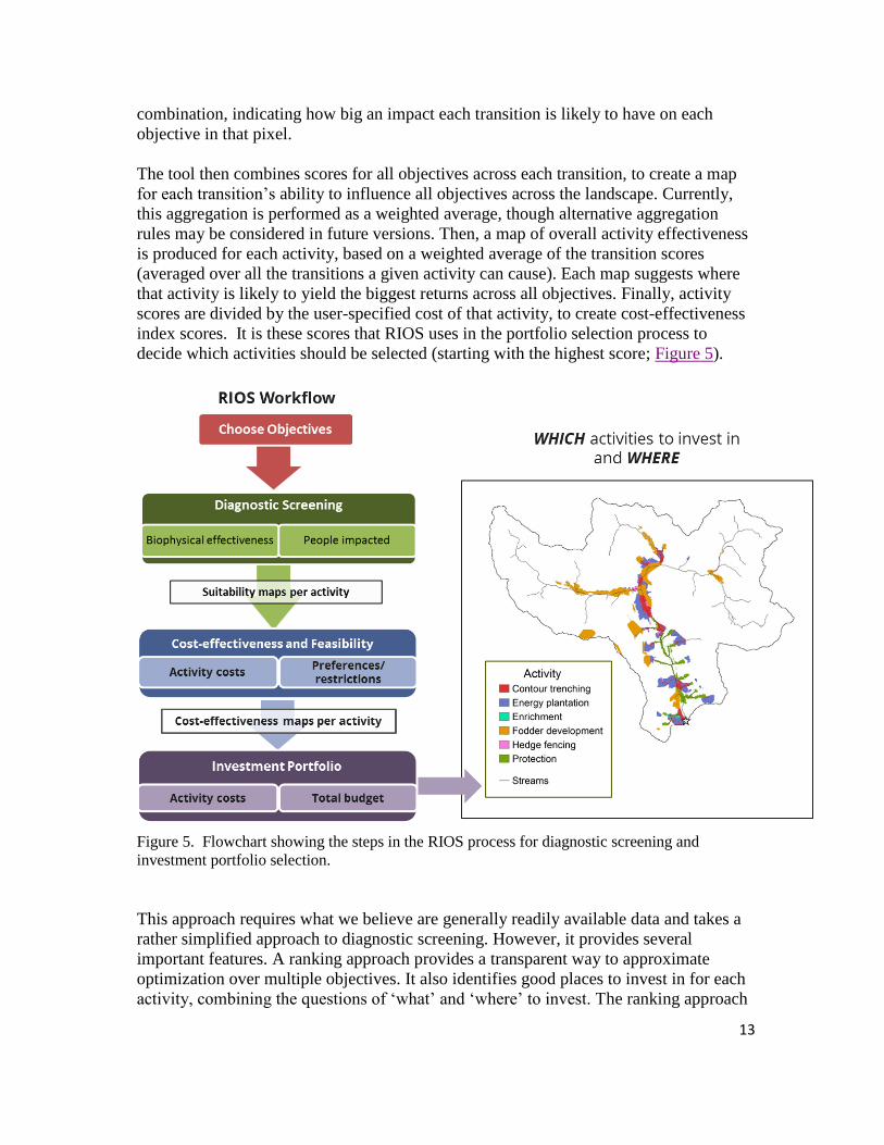
The tool then combines scores for all objectives across each transition, to create a map

for each transition’s ability to influence all objectives across the landscape. Currently,

this aggregation is performed as a weighted average, though alternative aggregation

rules may be considered in future versions. Then, a map of overall activity effectiveness

is produced for each activity, based on a weighted average of the transition scores

(averaged over all the transitions a given activity can cause). Each map suggests where

that activity is likely to yield the biggest returns across all objectives. Finally, activity

scores are divided by the user-specified cost of that activity, to create cost-effectiveness

index scores. It is these scores that RIOS uses in the portfolio selection process to

decide which activities should be selected (starting with the highest score; Figure 5).

Figure 5. Flowchart showing the steps in the RIOS process for diagnostic screening and

investment portfolio selection.

This approach requires what we believe are generally readily available data and takes a

rather simplified approach to diagnostic screening. However, it provides several

important features. A ranking approach provides a transparent way to approximate

optimization over multiple objectives. It also identifies good places to invest in for each

activity, combining the questions of ‘what’ and ‘where’ to invest. The ranking approach

14

also includes factors that represent landscape context, providing a simple method to

include some relatively complex and very important components of hydrological

processes. It also develops ranks based on the change the water fund is trying to make;

not only on the current condition of the watershed. Finally, the diagnostic screening

approach in RIOS, though simple, provides considerably more transparency than using

more sophisticated, quantitative models would.

Additional Portfolio Options

Weighting Objectives and Transitions

In the Objective Weights tab, users have the option to weight objectives and transitions

relative to each other. Default values assume that all objectives are considered equally

in determining the transition score, and that all transitions (land management changes)

contribute equally to fulfilling the objectives. Users may change the relative weights

between objectives, to indicate that some objectives should be considered more strongly

in the final selection of priority areas. Users can also change the relative weights

between transitions, to indicate that some transitions are more effective at achieving an

objective than others. For example, previous research from the study area may indicate

that keeping native vegetation is much more effective than restoration at improving dry

season baseflow and groundwater recharge. The weights are used to create a single

score per transition, by calculating a weighted average across all objectives.

Activity Preference Areas

Users can input spatial areas (GIS polygon shapefiles) where certain activities are either

preferred or should be prevented. If an area is preferred for an activity, RIOS will start

activity selection in that area, choosing the best places to invest in the preferred

activities first, before looking for best locations and activities in other areas. This means

that if an activity is preferred within an area, it may be selected by RIOS even if a

different activity (one that is not preferred) actually has a higher cost-effectiveness score

for the same pixel. If an activity is prevented within a given area, then that activity will

only be chosen for implementation outside of the area indicated.

Saving Parameter Files

Users have the option to save the input files associated with each run, and to load them

later when building a new portfolio. This allows users to quickly change only one or

two inputs, without having to re-enter all the inputs for each new portfolio. The Save

parameters and Load parameters from file options are found under the File menu in the

upper left corner of the RIOS window. Only parameter files saved with the User’s

current version of RIOS should be loaded, meaning that if a user created a portfolio with

version 0.4.5 and saved the parameter file, the parameter file can be loaded again using

v0.4.5, but cannot be loaded and used in later versions such as v1.0.0. Users that wish to

load parameter files from previous versions of RIOS should check all inputs carefully

before proceeding with the model run.

15

Budget Allocation

RIOS aims to help watershed investors spend money wisely to achieve their objectives,

and guides them towards practices and places that will yield the biggest return on

investment. There are often important social or political limitations on how money can

be spent, and that may change investors’ priorities away from economic efficiency as the

sole investment driver.

So RIOS provides two ways to specify how money is spent on activities. The first,

called a floating budget, is based on cost-effectiveness alone. The user provides a lump

sum value that RIOS may allocate among activities as it chooses, taking into account the

diagnostic screening scores and cost of each activity. While this will generate the most

cost-effective solution, it also is likely to heavily choose the least expensive activity,

producing a relatively non-diverse portfolio.

The second method of budget allocation is to specify an amount of money to be spent on

each individual activity. This method will produce a diverse portfolio, causing RIOS to

spend as much of the pre-allocated money as it can on each activity (still taking into

account the diagnostic screening score), in exchange for perhaps less economic

efficiency. Each of these methods (floating budget and per-activity allocation) may be

used alone, or both may be defined at the same time, such that RIOS will first spend pre-

allocated money on specific activities, then it will spend the floating budget in the most

cost-effective way in the area that remains. See the Select Budget section in the Step-by-

Step Guide for details on defining budgets in the tool.

RIOS users input the budget amount available to the fund, as well as the cost of each

activity. While some investors will want to see a single portfolio that indicates where

and in what activities to invest given the total budget amount, others may also want to

see how investments should proceed on an annual basis over the life of the fund. Users

have the option to define a total budget or an annual budget. If a total budget is defined,

one investment portfolio will be produced. If an annual budget is provided, one portfolio

will be produced for each year in succession.

Select Activity Portfolio

While the diagnostic screening process produces a view of the whole watershed

investment area, managers still need to know where to invest first. We refer to these

places as the ‘priority areas.’ The activity portfolio shows all of the priority areas

selected for each of the user-defined activities and objectives.

The number and extent of priority areas is determined by the size of the budget and/or

the targets set by the fund. The RIOS tool uses all previously described data inputs and

calculated outputs to identify where investments should be made first for a given budget

level. These inputs and preferences include:

16

1. Land use / land cover map

2. Table defining activities and indicating on which land cover types the activities

are allowed

3. Landscape factors that influence the effectiveness of transitions to achieve each

objective

4. The location and number of beneficiaries that benefit from activities in different

areas

5. Factor weights that describe the relative importance of each factor (and process)

6. Objective weights that assign a relative weight to objectives when multiple

objectives are considered

7. Activity-Transition table that indicates which user-defined activities cause which

transitions

8. Activity preference areas

9. Floating budget and/or budgets by activity

10. Activity costs

Inputs 1, 3, 4, 5, 6 are used to calculate weighted average scores for each transition.

These scores are used with input 7 to calculate weighted average scores for each activity.

Activity scores are divided by the activity cost (input 10) to produce an ROI raster for

each activity. Once the landscape constraints are met (inputs 2 and 8), selection of

priority areas is entirely driven by return on investment (ROI), where investments are

represented by activity costs and returns are determined by relative rankings. This

process is shown in Figure 6.

Activity costs can be input on either a per unit area or per unit length basis, and can be

as comprehensive as the user allows, (e.g., including opportunity costs of foregone

activities or direct incentives given to land managers to take on a given activity) and

should consider both implementation and maintenance costs. RIOS selects priority areas

by choosing the highest ROI pixels in order, until the defined budget (input 9) is spent.

The output of this step is the investment portfolio. If the user has specified an annual

budget for multiple years, RIOS will produce one portfolio per year. These portfolios

suggest the best places for the fund to invest in activities that have been identified to

achieve investors’ chosen objectives. Figure 7 gives two examples of RIOS investment

portfolios in Kenya and in India, created using different activities, budgets, and

preferences.

17

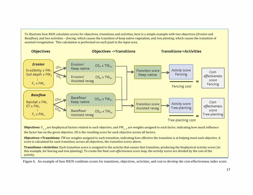
Figure 6. An example of how RIOS combines scores for transitions, objectives, activities, and cost to develop the cost-effectiveness index score.

Objectives: F1…n

are biophysical factors related to each objective, and FW1…n

are weights assigned to each factor, indicating how much influence

the factor has on the given objective. OS is the resulting score for each objective across all factors.

Objectives->Transitions: TW are weights assigned to each transition, indicating how effective the transition is at helping meet each objective. A

score is calculated for each transition, across all objectives, the transition scores above.

Transitions->Activities: Each transition score is assigned to the activity that causes that transition, producing the biophysical activity scores (in this example, for fencing and tree planting). To create the final cost-effectiveness score map, the activity scores are divided by the cost of the activity.

Objectives: F

1…n are biophysical factors related to each objective, and FW

1…n are weights assigned to each factor, indicating how much influence

the factor has on the given objective. OS is the resulting score for each objective across all factors.

Objectives->Transitions: TW are weights assigned to each transition, indicating how effective the transition is at helping meet each objective. A

score is calculated for each transition, across all objectives, the transition scores above.

Transitions->Activities: Each transition score is assigned to the activity that causes that transition, producing the biophysical activity scores for fencing and tree planting. To create the final cost-effectiveness score map, the activity scores are divided by the cost of the activity.

To illustrate how RIOS calculates scores for objectives, transitions and activities, here is a simple example with two objectives (Erosion and

Baseflow), and two activities – fencing, which causes the transition of keep native vegetation, and tree planting, which causes the transition of assisted revegetation. This calculation is performed on each pixel in the input area.

To get an idea of how RIOS calculates scores for objectives, transitions and activities, here is a simple example with two objectives (Erosion and

Baseflow), and two activities – fencing, which causes the transition of keep native vegetation, and tree planting, which causes the transition of

assisted revegetation.

18

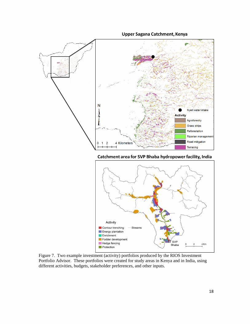
Figure 7. Two example investment (activity) portfolios produced by the RIOS Investment

Portfolio Advisor. These portfolios were created for study areas in Kenya and in India, using

different activities, budgets, stakeholder preferences, and other inputs.

19

Interpreting the Portfolio

Investment portfolios are a starting point for consideration by investors. Some

stakeholders may not agree with the location of priority areas or the budget allocation,

and further negotiation may be needed to reach a set of investments. Many desired

changes to the portfolio may be made by altering the options using the RIOS tool, while

others may not. The portfolios produced are likely to be just one input into the decision

making process.

A limitation of the portfolios currently produced with RIOS is its focus on land

management-based transitions. Many watershed investment funds will have other kinds

of activities they would like to invest in and objectives of importance that are not yet

included in the tool. In these cases, the portfolios RIOS produces can still serve to

represent a subset of interests and options that can help to inform further investment

prioritization discussions.

In general, the development of investment portfolios will likely be an iterative process

(Figure 8). Initial portfolios can be assessed in terms of the ecosystem service

improvements they provide by using the Portfolio Translator module and running

InVEST or other ecosystem services models on the resulting scenarios. If these impacts

are not as big as the fund had hoped, alternative portfolios can be created using larger

budgets, different activities and/or transitions. Much of the data used in RIOS can be

improved by local data gathered through expanding partnerships and a well-designed

monitoring program (Figure 8). As watershed managers gain a better understanding of

how activities actually impact transitions and objectives, any of the inputs to the

portfolio design may be altered to reflect this new knowledge.

20

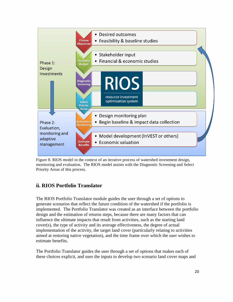
Figure 8. RIOS model in the context of an iterative process of watershed investment design,

monitoring and evaluation. The RIOS model assists with the Diagnostic Screening and Select

Priority Areas of this process.

ii. RIOS Portfolio Translator

The RIOS Portfolio Translator module guides the user through a set of options to

generate scenarios that reflect the future condition of the watershed if the portfolio is

implemented. The Portfolio Translator was created as an interface between the portfolio

design and the estimation of returns steps, because there are many factors that can

influence the ultimate impacts that result from activities, such as the starting land

cover(s), the type of activity and its average effectiveness, the degree of actual

implementation of the activity, the target land cover (particularly relating to activities

aimed at restoring native vegetation), and the time frame over which the user wishes to

estimate benefits.

The Portfolio Translator guides the user through a set of options that makes each of

these choices explicit, and uses the inputs to develop two scenario land cover maps and

21

associated biophysical parameter tables that are required to run the InVEST sediment

and water yield models. The two scenarios generated are:

1) the baseline land cover plus revegetation, agricultural management, and pasture

management activities implemented as new land cover-activity combinations

(called ‘transitioned’ in the output files); and

2) the above scenario plus areas that are “protected” have been transitioned to an

alternative land cover type (‘degraded’) as specified by the user (called

‘unprotected’ in the output files)

In order to create the scenarios and model input tables, the portfolio of activities output

by the Portfolio Advisor is divided into three different categories and each of these

categories is treated differently (Figure 9). The categories are:

a) Protection: Activities that achieve the transition Protect native vegetation

b) Restoration: Activities that achieve the transitions Revegetation – assisted or

Revegetation – unassisted

c) Agriculture: Activities that relate to Ditching, Fertilizer management, and

Pasture management

Figure 9. Schematic showing how the Portfolio Translator treats the three different categories of

transitions. The blue boxes labeled “RIOS” show information that is generated by the tool,

while the orange boxes labeled “User” represent information that the user must provide. RIOS

uses this information to build the biophysical tables for each of the two scenarios generated.

Protection: Protect Native Vegetation

The impacts of activities that protect native vegetation are calculated in reference to an

avoided (or degraded) transition, that is, what would happen in the absence of

protection. Users specify a land cover class that would most likely result in the absence

of protection. Users also specify the degree of transition to that new land cover,

providing a number between 0 and 1 to indicate the proportion that would be

transitioned. The proportional transition parameter allows users to adjust for the

probability that protected areas would be converted to the alternate land use in the

absence of protection, and is applied equally across the protected area – that is, RIOS

does not account for spatial differences in the probability of transition (for example

where some areas are more likely to convert than others). For the Portfolio Translator-

generated scenario 2 (described above), areas where protection activities occur are

assigned a new (degraded) land cover class, indicating the old LULC-activity

22

combination. Parameter values for the new land cover are determined as a percent

difference between the old and the avoided transition land cover’s parameter values, i.e.

𝑋𝑖 = 𝑋𝑜𝑙𝑑 + (𝑋𝑡𝑟𝑎𝑛𝑠 − 𝑋𝑜𝑙𝑑)𝑃

Where

𝑋𝑖 = Value of parameter X for the new (scenario 2) land cover

𝑋𝑜𝑙𝑑 = Value of parameter X for the original (baseline) land cover

𝑋𝑡𝑟𝑎𝑛𝑠 = Value of parameter X for the avoided transition land cover

𝑃 = Proportional transition (user specified)

Note: If you are not assessing a Protection-related activity, these inputs will still need to

be filled in and an ‘unprotected’ scenario map will be generated, but it will be identical

to the “transitioned” scenario and can be ignored.

Restoration: Revegetation – assisted and Revegetation – unassisted

The impacts of activities that restore vegetation are calculated in reference to the original

land cover and what the land is likely to be restored to. Users also specify the degree of

transition to that new land cover, providing a number between 0 and 1 indicating the

effectiveness of the restoration activity, or to what degree the area is transitioned to the

new land cover type within the target time frame. For the Portfolio Translator-generated

scenario 1 (described above), areas that are assigned revegetation-related activities are

assigned a new land cover, indicating the old LULC-transition-activity-new LULC

combination. The new LULC (final land cover type) is determined by the amount and

proximity of native vegetation in the surrounding area, as described below. This

approach assumes that the goal of revegetation is to restore areas to a land cover that is

similar to the closest and most abundant native land cover, and the results will reflect

this. If instead the goal of revegetation is to restore to a land cover that is not nearby, the

user will need to edit the resulting tables to reflect the desired land cover change.

When a pixel at location 𝑖, 𝑗 experiences a revegetation transition, we select the final

land cover type as the one that is most influenced by nearby native land cover types. We

define influence as a decaying exponential function of space as well as the total area of

native land cover type. Native land cover types are indicated in the LULC Biophysical

Coefficients table provided by the user (field name “native_veg”). The final land cover

type at 𝑖, 𝑗 is selected as the type that has the largest sum of exponential influence at

location 𝑖, 𝑗 over all possible native land cover types. Thus, a single neighboring pixel of

grassland may have less influence than the large number of forest pixels nearby. For

example, for a degraded area chosen for revegetation that is located close to a very small

area of grassland and a very large area of forest, the final land cover chosen will be

forest, and the new land cover description specified as “old LULC,

revegetation_assisted, revegetation, forest LULC.”

Formally, we define the native land cover type 𝑇 that has the most influence over pixel (𝑖, 𝑗) as,

23

𝑇(𝑖, 𝑗) = max𝜏 𝜖 all native land cover types ( ∑ 𝑚𝜏

all 𝑥,𝑦

(𝑥, 𝑦) ∙ 𝑒−

(𝑥−𝑖)2+(𝑦−𝑗)2

𝜎𝜏 )

Where

𝑚𝜏(𝑥, 𝑦) = {1, if pixel (𝑥, 𝑦) is land cover type 𝜏

0, otherwise

𝜎𝑖 the standard deviation of the Gaussian curve of influence for land cover type 𝑖

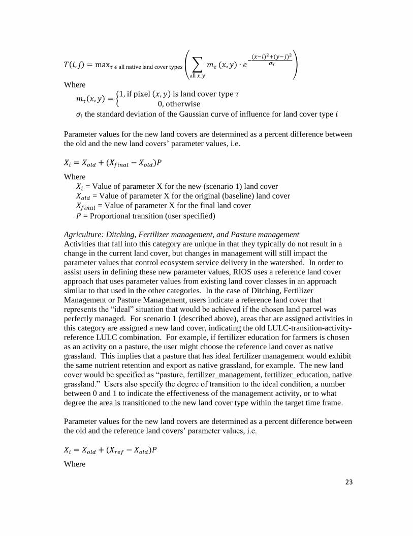
Parameter values for the new land covers are determined as a percent difference between

the old and the new land covers’ parameter values, i.e.

𝑋𝑖 = 𝑋𝑜𝑙𝑑 + (𝑋𝑓𝑖𝑛𝑎𝑙 − 𝑋𝑜𝑙𝑑)𝑃

Where



𝑋𝑓𝑖𝑛𝑎𝑙 = Value of parameter X for the final land cover


Agriculture: Ditching, Fertilizer management, and Pasture management

Activities that fall into this category are unique in that they typically do not result in a

change in the current land cover, but changes in management will still impact the

parameter values that control ecosystem service delivery in the watershed. In order to

assist users in defining these new parameter values, RIOS uses a reference land cover

approach that uses parameter values from existing land cover classes in an approach

similar to that used in the other categories. In the case of Ditching, Fertilizer

Management or Pasture Management, users indicate a reference land cover that

represents the “ideal” situation that would be achieved if the chosen land parcel was

perfectly managed. For scenario 1 (described above), areas that are assigned activities in

this category are assigned a new land cover, indicating the old LULC-transition-activity-

reference LULC combination. For example, if fertilizer education for farmers is chosen

as an activity on a pasture, the user might choose the reference land cover as native

grassland. This implies that a pasture that has ideal fertilizer management would exhibit

the same nutrient retention and export as native grassland, for example. The new land

cover would be specified as “pasture, fertilizer_management, fertilizer_education, native

grassland.” Users also specify the degree of transition to the ideal condition, a number

between 0 and 1 to indicate the effectiveness of the management activity, or to what

degree the area is transitioned to the new land cover type within the target time frame.

Parameter values for the new land covers are determined as a percent difference between

the old and the reference land covers’ parameter values, i.e.

𝑋𝑖 = 𝑋𝑜𝑙𝑑 + (𝑋𝑟𝑒𝑓 − 𝑋𝑜𝑙𝑑)𝑃

Where

24



𝑋𝑟𝑒𝑓 = Value of parameter X for the reference land cover


Number of years for transition

RIOS allows users to consider a specific time frame over which the effectiveness of

portfolio activities is to be assessed (the ‘Number of years for transition.’) For example,

for a given model run of RIOS, a user could run the Portfolio Translator multiple times

using different Proportional Transition (PT) values to indicate the expected level of

effectiveness for activities 5, 10, 20 and 50 years into the future, and run each output as

a model scenario to look at expected changes through time. Note that the ‘Number of

years for transition’ input is for user reference only, and is not used by the Portfolio

Translator in its calculations. Users should be aware of these assumptions and be

consistent in the application of PT values.

Summary

This method is intended to provide a general framework for how the effectiveness of

activities can be reflected in scenario parameter values (for the InVEST models) while

taking into account starting conditions, target conditions, and other assumptions. If

desired, users can include parameters for other InVEST models (such as nutrient

retention) in their biophysical coefficients table by adding these as additional columns.

The Portfolio Translator will interpolate all numerical values in the table using the same

procedures described above. Users are encouraged to review the biophysical

coefficients tables created by the Portfolio Translator, and to make corrections and

adjustments as needed based on local knowledge, conditions and the goals of the

scenario analysis.

iii. Estimating benefits of RIOS portfolios

The scenarios and biophysical tables generated by the RIOS Portfolio Translator module

provide users with data inputs needed to use InVEST models to evaluate changes in

water and sediment yield that result from portfolio implementation. The outputs from

the Portfolio Translator module are two scenarios of future change: one where all of the

activities are implemented on the landscape and any protected areas are actually

protected (so they retain their original land cover type, such as native forest; called

“transitioned” in the output files), and the other where all of the activities are

implemented BUT protected areas are degraded (changed to a degraded land cover type,

such as pasture; called “unprotected” in the output files). This allows users to calculate

not only the benefit of doing restoration, but also the marginal benefit from not allowing

the protected areas to degrade. If you are not assessing a Protection activity, then only

the benefit of doing restoration will be considered.

The differences in ecosystem services supply and value between the starting condition

and these scenarios provides the basis for understanding the impact of your investments

25

at a given level of budget.

The basic steps to perform this analysis are

1) Run the RIOS Investment Portfolio Advisor module to create your portfolios of

cost-effective interventions.

2) Run the RIOS Portfolio Translator module to generate the land cover scenarios

needed to represent changes from your activity portfolio. You will need a

baseline scenario (starting land cover), the transitioned scenario (activities +

protected areas unchanged), and unprotected scenario (activities + protected

areas degraded, if you included a Protection activity). Again, users are

encouraged to review these outputs and tailor them if needed to reflect local

knowledge and conditions.

3) Run the InVEST sediment retention and/or water yield models using as inputs

the land cover scenarios and biophysical tables produced by the Portfolio

Translator. You will run each InVEST model 3 times if including a Protection

activity, 2 times if not – once for each scenario.

4) Calculate the change in the InVEST model output of interest, following the

calculation shown in Figure 10. The calculation may be done at the level of the

entire watershed, or on sub-watershed outputs from InVEST.

Figure 10 gives an example of how benefits from portfolio implementation can be

estimated using RIOS outputs. If a Protection activity is included, and only the

differences in ES provision between the base land cover and the transitioned land cover

(ST) are calculated, it underestimates the true value of any protection activities because

protected areas are unchanged. Therefore, to get a true picture of the benefit you should

also calculate the marginal benefit of protection, by creating a scenario where protected

areas are converted to another (degraded) land cover (SU). The total ES returns from the

portfolio are then calculated as the benefits from restoration plus the marginal benefit

from protection. If a Protection-related activity is not assessed, then the benefit of

implementing the portfolio is the difference between ST and Base only.

26

Figure 10. Example of how benefits from investments could be calculated using outputs from

RIOS. The total ES returns from the portfolio are calculated as the benefits from restoration (ST

– Base) plus the marginal benefit from protection (ST – SU).

27

In ideal cases, water funds will state quantitative objectives, making it possible to define

the budget needed to most efficiently meet objectives, rather than starting with an

arbitrary budget and asking how much change it will achieve. Users can achieve this

with RIOS by setting an initial budget in the Portfolio Advisor, using the Portfolio

Translator to create implementation scenarios, running the relevant InVEST models to

compare the results to targets, and then modifying the budget in RIOS accordingly and

iterating through the process. Following this process through multiple iterations allows

users to zero in on the target budget level that most closely achieves the desired

outcomes in terms of ecosystem service benefit.

III. Model Descriptions

The following sections describe the impact models, input factors, and ranking

algorithms that are used for the diagnostic screening to select investment portfolios in

the RIOS tool.

i. Erosion Control for Drinking Water Quality and Reservoir Maintenance

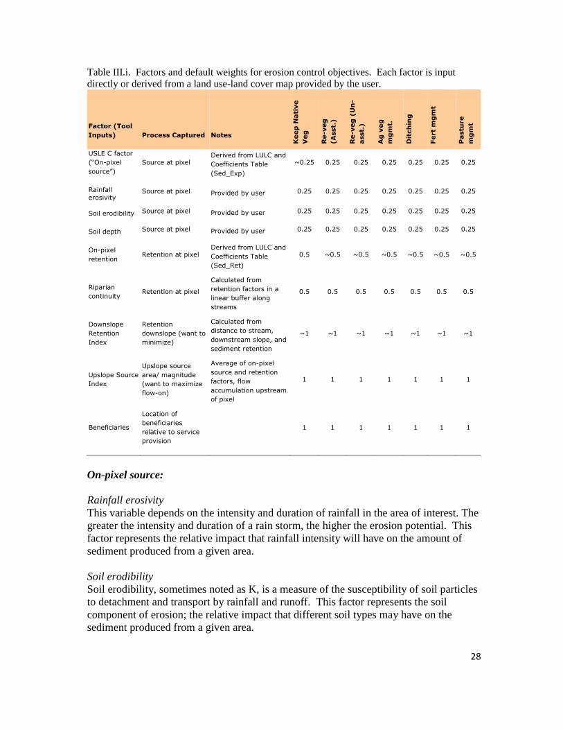
The primary factors derived from the literature review that influence erosion, sediment

export and retention are given in Table III.i and briefly described below. Default

weights are set in RIOS so that each major process (on-pixel source, retention, up- and

down-slope factors, and beneficiaries) is given equal weight when all factors are taken

together. For example, the factors USLE C factor, rainfall erosivity, soil erodibility, and

soil depth together represent the potential for activities to impact the on-pixel source of

sediment. Therefore these four factors are given weights of 0.25, which in sum results

in a weight of 1 for the on-pixel source process.

In the table that follows, values having a tilde (~) indicate that the given transition will

be more effective if activities are done on areas that currently have low values for that

factor. In other words, a higher score will be assigned to areas with low factor values.

Table values without a tilde indicate that the transition will be more effective on areas

with high values for that factor. Here, higher scores will be assigned to areas with high

factor values. For more information about how factors influence activity effectiveness,

see the Diagnostic Screening section.

28

Table III.i. Factors and default weights for erosion control objectives. Each factor is input

directly or derived from a land use-land cover map provided by the user.

Factor (Tool

Inputs) Process Captured Notes

Keep

Nati

ve

Veg

Re-v

eg

(A

sst.

)

Re-v

eg

(U

n-

asst.

)

Ag

veg

mg

mt.

Dit

ch

ing

Fert

mg

mt

Pastu

re

mg

mt

USLE C factor

(“On-pixel

source”)

Source at pixel Derived from LULC and

Coefficients Table

(Sed_Exp)

~0.25 0.25 0.25 0.25 0.25 0.25 0.25

Rainfall

erosivity Source at pixel Provided by user 0.25 0.25 0.25 0.25 0.25 0.25 0.25

Soil erodibility Source at pixel Provided by user 0.25 0.25 0.25 0.25 0.25 0.25 0.25

Soil depth Source at pixel Provided by user 0.25 0.25 0.25 0.25 0.25 0.25 0.25

On-pixel

retention Retention at pixel

Derived from LULC and

Coefficients Table

(Sed_Ret)

0.5 ~0.5 ~0.5 ~0.5 ~0.5 ~0.5 ~0.5

Riparian

continuity Retention at pixel

Calculated from

retention factors in a

linear buffer along

streams

0.5 0.5 0.5 0.5 0.5 0.5 0.5

Downslope

Retention

Index

Retention

downslope (want to

minimize)

Calculated from

distance to stream,

downstream slope, and

sediment retention

~1 ~1 ~1 ~1 ~1 ~1 ~1

Upslope Source

Index

Upslope source

area/ magnitude

(want to maximize

flow-on)

Average of on-pixel

source and retention

factors, flow

accumulation upstream

of pixel

1 1 1 1 1 1 1

Beneficiaries

Location of

beneficiaries

relative to service

provision

1 1 1 1 1 1 1

On-pixel source:

Rainfall erosivity

This variable depends on the intensity and duration of rainfall in the area of interest. The

greater the intensity and duration of a rain storm, the higher the erosion potential. This

factor represents the relative impact that rainfall intensity will have on the amount of

sediment produced from a given area.

Soil erodibility

Soil erodibility, sometimes noted as K, is a measure of the susceptibility of soil particles

to detachment and transport by rainfall and runoff. This factor represents the soil

component of erosion; the relative impact that different soil types may have on the

sediment produced from a given area.

29

Soil depth

The soil depth factor represents the total amount of sediment available for erosion and

transport down-slope. Areas with higher soil depth will have greater potential for soil

loss over time than those areas with shallow soil depth.

USLE C Factor (Average sediment export)

The Universal Soil Loss Equation uses the C factor, or crop factor, to represent the

susceptibility of each LULC type to erosion. An average C factor reported for different

land cover types is used to represent the contribution of land cover to determining the

relative erosion from a given area.

On-pixel retention:

Sediment retention

Sediment retention refers to the ability of a land parcel to hold sediment, thereby

preventing it from being transported and deposited further downstream. Retention

efficiencies vary by land cover class and are impacted by factors such as

geomorphology, climate, vegetative cover and management practices. A review of

literature yielded sediment retention efficiencies that can be used to represent the

contribution of land cover to determining the relative retention for a given area.

Riparian continuity

The effectiveness of restoration or protection activities in riparian areas is highly

correlated with their continuity. While the retention downslope from an area is a key

factor in determining the relative effectiveness of an activity on riparian pixels, the

linear retention along the stream channel is most critical for determining relative

impacts. Continuous riparian buffers are the most effective at maintaining or restoring

sediment and nutrient retention. Therefore, an activity will be most effective at

controlling sediment load to a river if it results in a formerly discontinuous buffer being

made continuous.

Downslope Retention Index

The downslope retention index describes the relative retention ability of the area

downslope of a given pixel. Because activities will have the most impact on areas with

little downslope retention, we want to minimize this factor. The downslope retention

index is calculated as a weighted flow length, using slope and sediment retention factors

as weights.

Upslope Source Index

The upslope source index describes the source area and magnitude of the source

reaching a pixel, a factor that is cited frequently as an indicator of the effectiveness of an

activity for influencing erosion control. Because activities will be most effective if

performed in an area with a large upslope sediment source, we want to maximize this

factor. The upslope source index is calculated as a weighted flow accumulation, using

an average of all the on-pixel source factors, retention factors, and slope.

30

Beneficiaries

Beneficiaries represent the value people receive from an ecosystem service. When

evaluating potential activity locations and returns, it is important to consider the number

of beneficiaries that are gaining from the preservation of natural capital in that area. For

example, beneficiaries of erosion control for drinking water quality could be the number

of people that rely on water produced in that watershed. The beneficiaries of erosion

control for reservoir maintenance could be the number of people that rely on that

reservoir for their water supply, the number of kilowatt-hours of electricity produced, or

a representation of added value in some other metric.

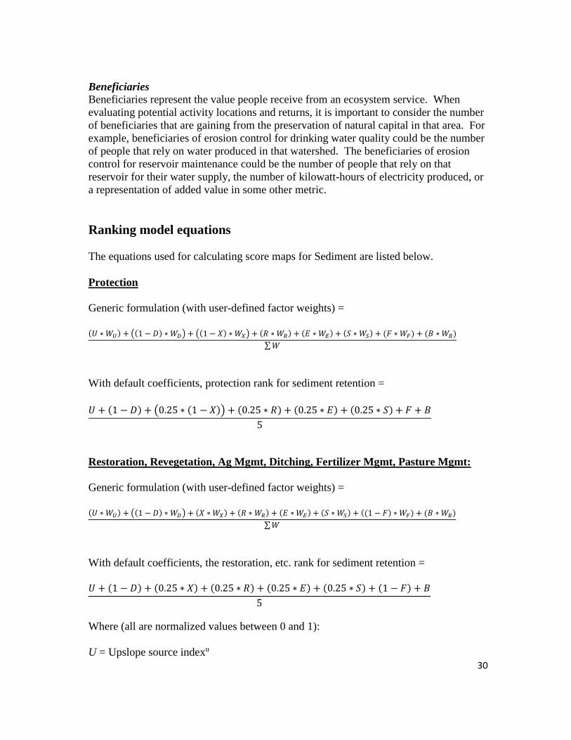
Ranking model equations

The equations used for calculating score maps for Sediment are listed below.

Protection

Generic formulation (with user-defined factor weights) = (𝑈 ∗ 𝑊𝑈) + ((1 − 𝐷) ∗ 𝑊𝐷) + ((1 − 𝑋) ∗ 𝑊𝑋) + (𝑅 ∗ 𝑊𝑅) + (𝐸 ∗ 𝑊𝐸) + (𝑆 ∗ 𝑊𝑆) + (𝐹 ∗ 𝑊𝐹) + (𝐵 ∗ 𝑊𝐵)

∑ 𝑊

With default coefficients, protection rank for sediment retention =

𝑈 + (1 − 𝐷) + (0.25 ∗ (1 − 𝑋)) + (0.25 ∗ 𝑅) + (0.25 ∗ 𝐸) + (0.25 ∗ 𝑆) + 𝐹 + 𝐵

5

Restoration, Revegetation, Ag Mgmt, Ditching, Fertilizer Mgmt, Pasture Mgmt:

Generic formulation (with user-defined factor weights) = (𝑈 ∗ 𝑊𝑈) + ((1 − 𝐷) ∗ 𝑊𝐷) + (𝑋 ∗ 𝑊𝑋) + (𝑅 ∗ 𝑊𝑅) + (𝐸 ∗ 𝑊𝐸) + (𝑆 ∗ 𝑊𝑆) + ((1 − 𝐹) ∗ 𝑊𝐹) + (𝐵 ∗ 𝑊𝐵)

∑ 𝑊

With default coefficients, the restoration, etc. rank for sediment retention = 𝑈 + (1 − 𝐷) + (0.25 ∗ 𝑋) + (0.25 ∗ 𝑅) + (0.25 ∗ 𝐸) + (0.25 ∗ 𝑆) + (1 − 𝐹) + 𝐵

5

Where (all are normalized values between 0 and 1):

U = Upslope source indexu

31

D = Downslope retention indexd

X = Sediment export coefficient

R = Erosivity coefficient

E = Erodibility coefficient

S = Soil depth

F = Final retention index

If pixel is NOT riparian, F = Sediment retention coefficient

Else, F = (Sediment retention + Riparian continuity index)/2

B = Beneficiaries index

WN = Weight assigned to each factor

u Upslope source index is calculated as the accumulated weight (sum) of all cells

flowing into each downslope cell in the output raster. The weight of the xth cell is a

function of the factors controlling export and retention on the cells that flow into the xth

cell.

𝑈𝑥 = 𝑊𝑥 + ∑ 𝑈𝑖

𝑖∈{𝑖𝑛𝑓𝑙𝑜𝑤𝑖𝑛𝑔 𝑛𝑒𝑖𝑔ℎ𝑏𝑜𝑟𝑠 𝑜𝑛 𝑥}

𝑊𝑥 =𝐴𝑥 + 𝑋𝑥 + 𝑅𝑥 + 𝐸𝑥 + 𝑆𝑥 + (1 − 𝐹𝑥)

6

Where

Ux = Upslope source index of cell x

Wx = Weight assigned to cell x

Ax = Slope index (normalized values between 0 and 1)

Xx = Sediment export coefficient (normalized values between 0 and 1)

Rx = Erosivity coefficient (normalized values between 0 and 1)

Ex = Erodibility coefficient (normalized values between 0 and 1)

Sx = Soil depth (normalized values between 0 and 1)

Fx = Final retention index (normalized values between 0 and 1)

If pixel is NOT riparian, F = Sediment retention coefficient

Else, F = (Sediment retention + Riparian continuity index)/2

d Downslope retention index is calculated as the downstream weighted distance along

the flow path for each cell. The stream network is first assigned a null value in the flow

direction raster, so the downstream weighted distance is calculated from each cell to the

nearest stream. The weight of the xth cell is a function of the retention factors of the

cells along the flow path.

𝐷𝑥 = 𝑊𝑥𝐿𝑥 + 𝐷𝑜𝑢𝑡𝑓𝑙𝑜𝑤𝑥

𝑊𝑥 =(1 − 𝐴𝑥) + 𝑅𝑒𝑡𝑥

2

32

Where

Dx = Downslope retention index of cell x


Lx = Length of cell x


Retx = Sediment retention coefficient (normalized values between 0 and 1)

ii. Nutrient Retention: Phosphorus

The primary factors derived from the literature review that influence phosphorus export

and retention are given in Table III.ii and briefly described below. Because sources of

phosphorus that impact drinking water quality are primarily transported with sediments

(as opposed to dissolved in surface or sub-surface runoff), the factors for the Phosphorus

Retention Impact Ranking Model are the same as for Erosion Control. Default weights

are set so that each major process (on-pixel source, retention, up- and down-slope

factors, and beneficiaries) is given equal weight when all factors are taken together. For

example, the factors phosphorus export, rainfall erosivity, soil erodibility, and soil depth

together represent the potential for activities to impact the on-pixel source of

phosphorus. Therefore these four factors are given weights of 0.25, which in sum

results in a weight of 1 for the on-pixel source process.



factor. In other words, higher rank will be assigned to areas with low factor values.


with high values for that factor. Here, higher rank will be assigned to areas with high



Table III.ii. Factors and default weights for phosphorus retention. Each factor is input directly

or derived from a land use-land cover map provided by the user.

Factor (Tool


Keep

Nati

ve

Veg

Re-v

eg

(A

sst.

)

Re-v

eg

(U

n-

asst.

)

Ag

veg

mg

mt.

Dit

ch

ing

Fert

mg

mt

Pastu

re

mg

mt

On-pixel

source Source at pixel


Coefficients Table

(P_Exp)

~0.25 0.25 0.25 0.25 0.25 0.25 0.25

Rainfall

erosivity Source at pixel Provided by user 0.25 0.25 0.25 0.25 0.25 0.25 0.25

Soil erodibility Source at pixel Provided by user 0.25 0.25 0.25 0.25 0.25 0.25 0.25


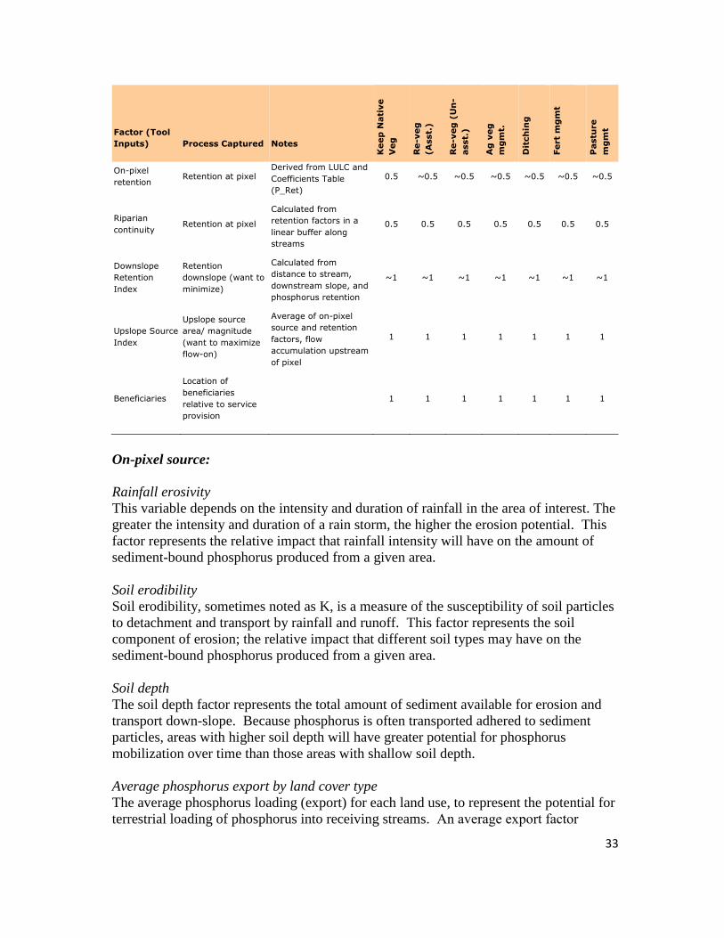
33

Factor (Tool


Keep

Nati

ve

Veg

Re-v

eg

(A

sst.

)

Re-v

eg

(U

n-

asst.

)

Ag

veg

mg

mt.

Dit

ch

ing

Fert

mg

mt

Pastu

re

mg

mt

On-pixel



Coefficients Table

(P_Ret)

0.5 ~0.5 ~0.5 ~0.5 ~0.5 ~0.5 ~0.5

Riparian


Calculated from


linear buffer along

streams

0.5 0.5 0.5 0.5 0.5 0.5 0.5

Downslope

Retention

Index

Retention

downslope (want to

minimize)

Calculated from

distance to stream,


phosphorus retention

~1 ~1 ~1 ~1 ~1 ~1 ~1

Upslope Source

Index

Upslope source

area/ magnitude

(want to maximize

flow-on)

Average of on-pixel


factors, flow


of pixel

1 1 1 1 1 1 1

Beneficiaries

Location of

beneficiaries

relative to service

provision

1 1 1 1 1 1 1

On-pixel source:

Rainfall erosivity

This variable depends on the intensity and duration of rainfall in the area of interest. The

greater the intensity and duration of a rain storm, the higher the erosion potential. This

factor represents the relative impact that rainfall intensity will have on the amount of

sediment-bound phosphorus produced from a given area.

Soil erodibility

Soil erodibility, sometimes noted as K, is a measure of the susceptibility of soil particles

to detachment and transport by rainfall and runoff. This factor represents the soil

component of erosion; the relative impact that different soil types may have on the

sediment-bound phosphorus produced from a given area.

Soil depth

The soil depth factor represents the total amount of sediment available for erosion and

transport down-slope. Because phosphorus is often transported adhered to sediment

particles, areas with higher soil depth will have greater potential for phosphorus

mobilization over time than those areas with shallow soil depth.

Average phosphorus export by land cover type

The average phosphorus loading (export) for each land use, to represent the potential for

terrestrial loading of phosphorus into receiving streams. An average export factor

34

reported for different land cover types is used to represent the contribution of land cover

to determining the source of phosphorus from a given area.

On-pixel retention:

Phosphorus retention

Phosphorus retention efficiencies vary by land cover class. A review of literature

yielded P retention efficiencies that can be used to represent the contribution of land

cover to determining the relative retention for a given area.

Riparian continuity








made continuous.



downslope of a given pixel. Because activities will be most effective if performed in an

area with little downslope retention, we want to minimize this factor. The downslope

retention index is calculated as a weighted flow length, using slope and phosphorus

retention factors as weights.


The upslope source index describes the area and magnitude of the source reaching a

pixel, a factor that is cited frequently as an indicator of the effectiveness of an activity

for influencing nutrient retention. Because activities will be most effective if performed

in an area with a large upslope phosphorus source, we want to maximize this factor. The

upslope source index is calculated as a weighted flow accumulation, using an average of

all the on-pixel source factors, retention factors, and slope.

Beneficiaries

Beneficiaries are an important factor for evaluating the impacts of activities on any

ecosystem service, because they represent the ultimate benefit derived from the service.

When evaluating potential activity locations and returns, it is important to consider the

number of beneficiaries that benefit from the natural capital in that area. When

considering phosphorus retention for drinking water quality, the beneficiaries could be

the number of people that rely on water produced in that watershed.

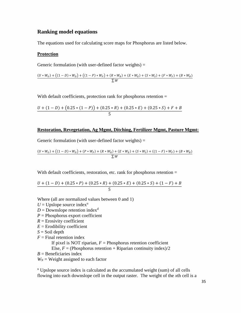
35


The equations used for calculating score maps for Phosphorus are listed below.

Protection

Generic formulation (with user-defined factor weights) =

(𝑈 ∗ 𝑊𝑈) + ((1 − 𝐷) ∗ 𝑊𝐷) + ((1 − 𝑃) ∗ 𝑊𝑃) + (𝑅 ∗ 𝑊𝑅) + (𝐸 ∗ 𝑊𝐸) + (𝑆 ∗ 𝑊𝑆) + (𝐹 ∗ 𝑊𝐹) + (𝐵 ∗ 𝑊𝐵)

∑ 𝑊

With default coefficients, protection rank for phosphorus retention =

𝑈 + (1 − 𝐷) + (0.25 ∗ (1 − 𝑃)) + (0.25 ∗ 𝑅) + (0.25 ∗ 𝐸) + (0.25 ∗ 𝑆) + 𝐹 + 𝐵

5


Generic formulation (with user-defined factor weights) = (𝑈 ∗ 𝑊𝑈) + ((1 − 𝐷) ∗ 𝑊𝐷) + (𝑃 ∗ 𝑊𝑃) + (𝑅 ∗ 𝑊𝑅) + (𝐸 ∗ 𝑊𝐸) + (𝑆 ∗ 𝑊𝑆) + ((1 − 𝐹) ∗ 𝑊𝐹) + (𝐵 ∗ 𝑊𝐵)

∑ 𝑊

With default coefficients, restoration, etc. rank for phosphorus retention = 𝑈 + (1 − 𝐷) + (0.25 ∗ 𝑃) + (0.25 ∗ 𝑅) + (0.25 ∗ 𝐸) + (0.25 ∗ 𝑆) + (1 − 𝐹) + 𝐵

5

Where (all are normalized values between 0 and 1)

U = Upslope source indexu

D = Downslope retention indexd

P = Phosphorus export coefficient

R = Erosivity coefficient

E = Erodibility coefficient

S = Soil depth


If pixel is NOT riparian, F = Phosphorus retention coefficient

Else, F = (Phosphorus retention + Riparian continuity index)/2





36


cell.



𝑊𝑥 =𝐴𝑥 + 𝑋𝑥 + 𝑅𝑥 + 𝐸𝑥 + 𝑆𝑥 + (1 − 𝐹𝑥)

6

Where




Px = Phosphorus export coefficient (normalized values between 0 and 1)

Rx = Erosivity coefficient (normalized values between 0 and 1)

Ex = Erodibility coefficient (normalized values between 0 and 1)



If pixel is NOT riparian, F = Phosphorus retention coefficient

Else, F = (Phosphorus retention + Riparian continuity index)/2








2

Where





Retx = Phosphorus retention coefficient (normalized values between 0 and 1)

iii. Nutrient Retention: Nitrogen

The primary briefly factors derived from the literature review that influence nitrogen

export and retention are given in Table III.iii and described below. Because sources of

nitrogen that impact drinking water quality are often dissolved in surface and sub-

surface flows, the factors for the Nitrogen Retention Impact Ranking Model focus on the

export and retention of nitrogen as measured in experimental and modeling studies that

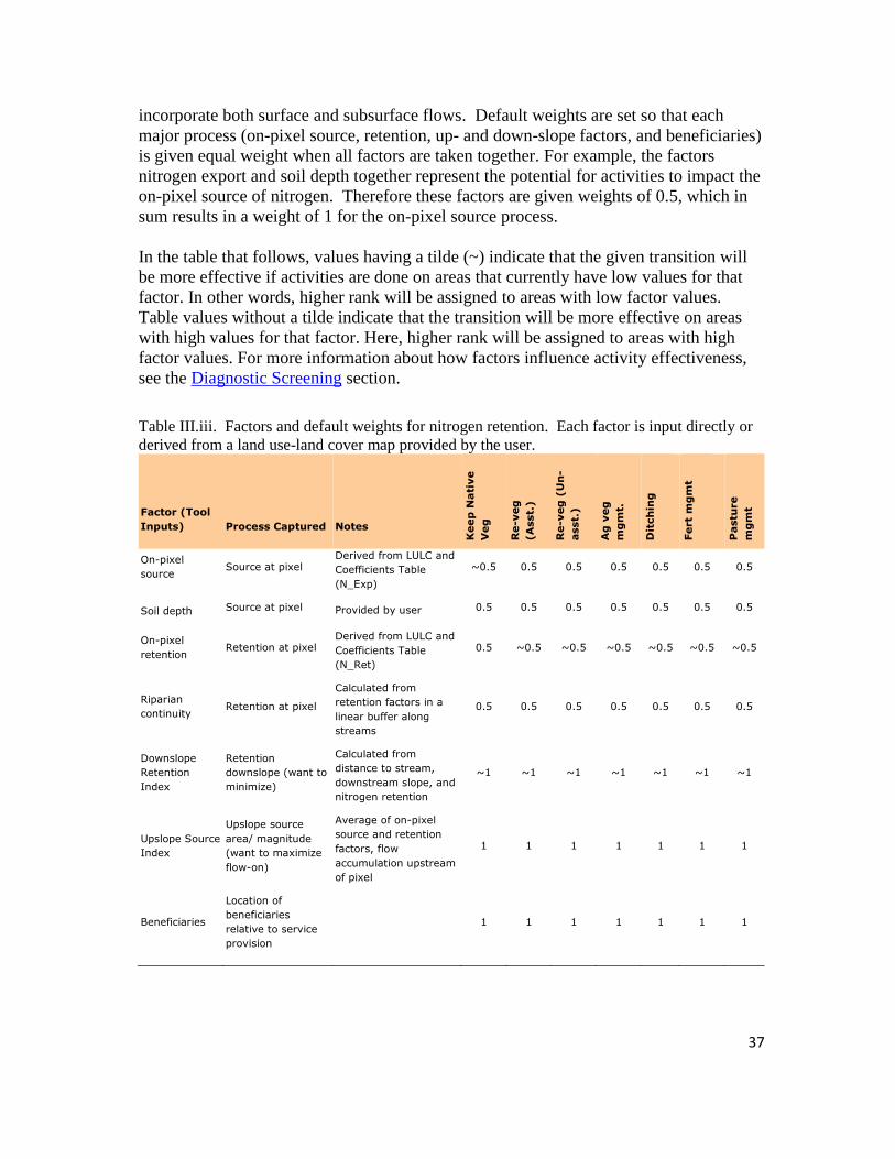
37

incorporate both surface and subsurface flows. Default weights are set so that each

major process (on-pixel source, retention, up- and down-slope factors, and beneficiaries)

is given equal weight when all factors are taken together. For example, the factors

nitrogen export and soil depth together represent the potential for activities to impact the

on-pixel source of nitrogen. Therefore these factors are given weights of 0.5, which in

sum results in a weight of 1 for the on-pixel source process.








Table III.iii. Factors and default weights for nitrogen retention. Each factor is input directly or

derived from a land use-land cover map provided by the user.

Factor (Tool


Keep

Nati

ve

Veg

Re-v

eg

(A

sst.

)

Re-v

eg

(U

n-

asst.

)

Ag

veg

mg

mt.

Dit

ch

ing

Fert

mg

mt

Pastu

re

mg

mt

On-pixel

source Source at pixel


Coefficients Table

(N_Exp)

~0.5 0.5 0.5 0.5 0.5 0.5 0.5


On-pixel



Coefficients Table

(N_Ret)

0.5 ~0.5 ~0.5 ~0.5 ~0.5 ~0.5 ~0.5

Riparian


Calculated from


linear buffer along

streams

0.5 0.5 0.5 0.5 0.5 0.5 0.5

Downslope

Retention

Index

Retention

downslope (want to

minimize)

Calculated from

distance to stream,


nitrogen retention

~1 ~1 ~1 ~1 ~1 ~1 ~1

Upslope Source

Index

Upslope source

area/ magnitude

(want to maximize

flow-on)

Average of on-pixel


factors, flow


of pixel

1 1 1 1 1 1 1

Beneficiaries

Location of

beneficiaries

relative to service

provision

1 1 1 1 1 1 1

38

On-pixel source:

Soil depth

The soil depth factor impacts the total amount of nitrogen available for export from a

pixel. Areas with higher soil depth will have greater potential for nitrogen export over

time than those areas with shallow soil depth.

Average nitrogen export by land cover type

The average nitrogen loading (export) for each land use, to represent the potential for

terrestrial loading of nitrogen into receiving streams. An average export factor reported

for different land cover types is used to represent the contribution of land cover to

determining the source of nitrogen from a given area.

On-pixel retention:

Nitrogen retention

Nitrogen retention efficiencies vary by land cover class. A review of literature yielded

N retention efficiencies that can be used to represent the contribution of land cover to

determining the relative retention for a given area.

Riparian continuity








made continuous.



downslope of a given pixel. Because activities will be most effective if performed in an

area with little downslope retention, we want to minimize this factor. The downslope

retention index is calculated as a weighted flow length, using slope and nitrogen

retention factors as weights.


The upslope source index describes the source area and magnitude of the source

reaching a pixel, a factor that is cited frequently as an indicator of the effectiveness of an

activity for influencing nitrogen retention. Because activities will be most effective if

performed in an area with a large upslope nitrogen source, we want to maximize this

factor. The upslope source index is calculated as a weighted flow accumulation, using

an average of all the on-pixel source factors, retention factors, and slope.

Beneficiaries


39




considering nitrogen retention for drinking water quality, the beneficiaries could be the

number of people that rely on water produced in that watershed.


The equations used for calculating score maps for Nitrogen are listed below.

Protection


(𝑈 ∗ 𝑊𝑈) + ((1 − 𝐷) ∗ 𝑊𝐷) + ((1 − 𝑁) ∗ 𝑊𝑁) + (𝑆 ∗ 𝑊𝑆) + (𝐹 ∗ 𝑊𝐹) + (𝐵 ∗ 𝑊𝐵)

∑ 𝑊

With default coefficients, protection rank for nitrogen retention =

𝑈 + (1 − 𝐷) + (0.5 ∗ (1 − 𝑁)) + (0.5 ∗ 𝑆) + 𝐹 + 𝐵

5



(𝑈 ∗ 𝑊𝑈) + ((1 − 𝐷) ∗ 𝑊𝐷) + (𝑁 ∗ 𝑊𝑁) + (𝑆 ∗ 𝑊𝑆) + ((1 − 𝐹) ∗ 𝑊𝐹) + (𝐵 ∗ 𝑊𝐵)

∑ 𝑊

With default coefficients, restoration, etc. rank for nitrogen retention = 𝑈 + (1 − 𝐷) + (0.5 ∗ 𝑁) + (0.5 ∗ 𝑆) + (1 − 𝐹) + 𝐵

5


U = Upslope source index

D = Downslope retention index

N = Nitrogen export coefficient

S = Soil depth


If pixel is NOT riparian, F = Nitrogen retention coefficient

Else, F = (Nitrogen retention + Riparian continuity index)/2

40






cell.



𝑊𝑥 =𝐴𝑥 + 𝑁𝑥 + 𝑆𝑥 + (1 − 𝐹𝑥)

4

Where




Nx = Nitrogen export coefficient (normalized values between 0 and 1)



If pixel is NOT riparian, F = Nitrogen retention coefficient

Else, F = (Nitrogen retention + Riparian continuity index)/2








2

Where





Retx = Nitrogen retention coefficient (normalized values between 0 and 1)

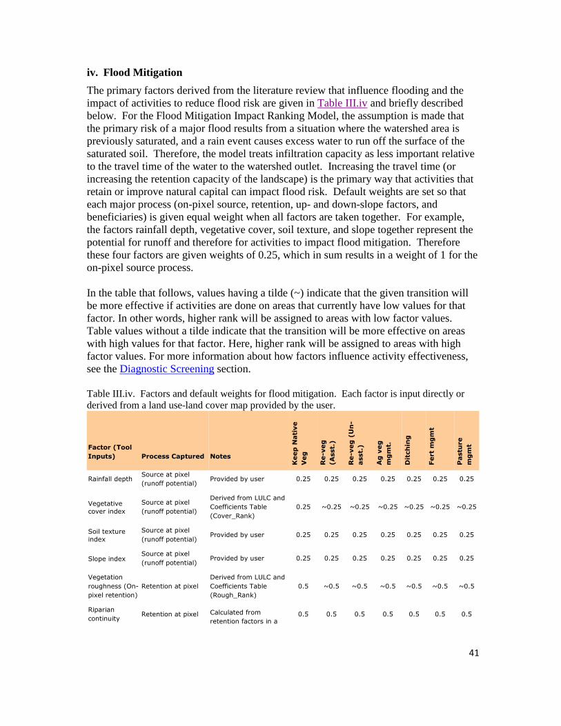
41

iv. Flood Mitigation

The primary factors derived from the literature review that influence flooding and the

impact of activities to reduce flood risk are given in Table III.iv and briefly described

below. For the Flood Mitigation Impact Ranking Model, the assumption is made that

the primary risk of a major flood results from a situation where the watershed area is

previously saturated, and a rain event causes excess water to run off the surface of the

saturated soil. Therefore, the model treats infiltration capacity as less important relative

to the travel time of the water to the watershed outlet. Increasing the travel time (or

increasing the retention capacity of the landscape) is the primary way that activities that

retain or improve natural capital can impact flood risk. Default weights are set so that

each major process (on-pixel source, retention, up- and down-slope factors, and

beneficiaries) is given equal weight when all factors are taken together. For example,

the factors rainfall depth, vegetative cover, soil texture, and slope together represent the

potential for runoff and therefore for activities to impact flood mitigation. Therefore

these four factors are given weights of 0.25, which in sum results in a weight of 1 for the

on-pixel source process.








Table III.iv. Factors and default weights for flood mitigation. Each factor is input directly or

derived from a land use-land cover map provided by the user.

Factor (Tool


Keep

Nati

ve

Veg

Re-v

eg

(A

sst.

)

Re-v

eg

(U

n-

asst.

)

Ag

veg

mg

mt.

Dit

ch

ing

Fert

mg

mt

Pastu

re

mg

mt

Rainfall depth Source at pixel

(runoff potential) Provided by user 0.25 0.25 0.25 0.25 0.25 0.25 0.25

Vegetative

cover index

Source at pixel

(runoff potential)


Coefficients Table

(Cover_Rank)

0.25 ~0.25 ~0.25 ~0.25 ~0.25 ~0.25 ~0.25

Soil texture

index

Source at pixel


Slope index Source at pixel


Vegetation

roughness (On-

pixel retention)

Retention at pixel


Coefficients Table

(Rough_Rank)

0.5 ~0.5 ~0.5 ~0.5 ~0.5 ~0.5 ~0.5

Riparian

continuity Retention at pixel Calculated from

retention factors in a 0.5 0.5 0.5 0.5 0.5 0.5 0.5

42

Factor (Tool


Keep

Nati

ve

Veg

Re-v

eg

(A

sst.

)

Re-v

eg

(U

n-

asst.

)

Ag

veg

mg

mt.

Dit

ch

ing

Fert

mg

mt

Pastu

re

mg

mt

linear buffer along

streams

Downslope

Retention

Index

Retention

downslope (want to

minimize)

Calculated from

distance to stream,


vegetation roughness

~1 ~1 ~1 ~1 ~1 ~1 ~1

Upslope Source

Index

Upslope source

area/ magnitude

(want to maximize

flow-on)

Average of on-pixel


factors, flow


of pixel

1 1 1 1 1 1 1

Beneficiaries

Location of

beneficiaries

relative to service

provision

1 1 1 1 1 1 1

On-pixel source:

The on-pixel source factors for flooding are those that describe runoff magnitude. The

factors used to represent runoff magnitude here are derived from a method developed by

the FAO that relates runoff depth for a given storm to rainfall, soil texture, vegetative

cover, and slope.

Rainfall Depth

Rainfall depth influences the amount of runoff produced from a given pixel. Ideally, the

average rainfall depth of a given return period storm event would be provided by the

user. As a proxy, we recommend using Average Precipitation of Wettest Month, which

is a statistic available globally from the WorldClim database.

Soil Texture

Soil texture is an important factor that impacts how well water infiltrates through the soil

surface. Texture relates to the size of soil particles and the size of pore space through

which water can infiltrate. Soils with very fine texture (i.e. clays) are more likely to

cause runoff than soils with a coarser texture (i.e. sands).

Slope index

Slope is used in this model to represent the potential for rainfall to run over the soil

surface during rainfall events rather than infiltrating. Areas with a higher slope tend to

have greater runoff, and therefore more potential to cause downstream flooding.

Vegetative Cover

The percent soil covered by vegetation is an important factor that impacts the amount of

rainfall interception and potential infiltration during rainfall events. Areas with a greater

percentage of vegetative cover tend to have greater rainfall interception and higher

http://worldclim.org/current

43

potential for infiltration, therefore producing less runoff.

On-pixel retention:

Manning’s n Roughness

Manning’s n coefficient describes the surface roughness related to the type of vegetation

present. The roughness coefficient is related to the resistance that water encounters as it

travels across the surface as overland flow, and so is used in the Flood Mitigation

Ranking Model as a proxy for on-pixel retention.

Riparian continuity





impacts. For flood mitigation, the most effective riparian buffers are those that are

continuous. An activity will be more effective at slowing overland flow towards a river

if the activity results in a formerly discontinuous buffer being made continuous.


The downslope retention index describes the relative ability of the area downslope of a

given pixel to retard flow velocity. Because activities will be most effective if

performed in an area with little downslope retention, we want to minimize this factor.

The downslope retention index is calculated as a weighted flow length, using slope and

the roughness (n) coefficient as weights.


The upslope source index describes the source area and magnitude of the runoff reaching

a pixel. Because activities to mitigate flood risk will be most effective if performed in

an area with a large upslope runoff source, we want to maximize this factor. The

upslope source index is calculated as a weighted flow accumulation, using an average of

all the on-pixel source factors, retention factors, and slope.

Beneficiaries





considering flood mitigation, the beneficiaries could be the number of people that reside

in the floodplain, or the value of property at risk from large flood events that originate in

the watershed.

44


The equations used for calculating score maps for Flood Mitigation are listed below.

Protection


(𝑈 ∗ 𝑊𝑈) + ((1 − 𝐷) ∗ 𝑊𝐷) + (𝑃𝑟 ∗ 𝑊𝑃𝑟) + (𝐶 ∗ 𝑊𝐶) + ((1 − 𝑇) ∗ 𝑊𝑇) + (𝑆𝑙 ∗ 𝑊𝑆𝑙) + (𝐹 ∗ 𝑊𝐹) + (𝐵 ∗ 𝑊𝐵)

∑ 𝑊

With default coefficients, protection rank for flood mitigation =

𝑈 + (1 − 𝐷) + (0.25 ∗ 𝑃𝑟) + (0.25 ∗ 𝐶) + (0.25 ∗ (1 − 𝑇)) + (0.25 ∗ 𝑆𝑙) + 𝐹 + 𝐵

5


Generic formulation (with user-defined factor weights) = (𝑈 ∗ 𝑊𝑈) + ((1 − 𝐷) ∗ 𝑊𝐷) + (𝑃𝑟 ∗ 𝑊𝑃𝑟) + ((1 − 𝐶) ∗ 𝑊𝐶) + (𝑇 ∗ 𝑊𝑇) + (𝑆𝑙 ∗ 𝑊𝑆𝑙) + ((1 − 𝐹) ∗ 𝑊𝐹) + (𝐵 ∗ 𝑊𝐵)

∑ 𝑊

With default coefficients, restoration, etc. rank for flood mitigation = 𝑈 + (1 − 𝐷) + (0.25 ∗ 𝑃𝑟) + (0.25 ∗ (1 − 𝐶)) + (0.25 ∗ 𝑇) + (0.25 ∗ 𝑆𝑙) + (1 − 𝐹) + 𝐵

5




Pr = Precipitation of wettest month

C = Vegetation cover index

T = Soil texture index

Sl = Slope index


If pixel is NOT riparian, F = Vegetation roughness coefficient

Else, F = (Vegetation roughness coefficient + Riparian continuity index)/2





45

function of the factors controlling flow and infiltration on the cells that flow into the xth

cell.



𝑊𝑥 =𝑃𝑟𝑥 +(1 − 𝐶𝑥) + 𝑇𝑥 + 𝑆𝑙𝑥 + (1 − 𝐹𝑥)

5

Where



Prx = Precipitation of wettest month (normalized values between 0 and 1)

Cx = Vegetation cover index (normalized values between 0 and 1)

Tx = Soil texture index (normalized values between 0 and 1)

Slx = Slope index (normalized values between 0 and 1)


If pixel is NOT riparian, F = Vegetation roughness coefficient

Else, F = (Vegetation roughness coefficient + Riparian continuity index)/2




nearest stream. The weight of the xth cell is a function of the flow retention factors of

the cells along the flow path.


𝑊𝑥 =(1 − 𝑆𝑙𝑥) + 𝑅𝑒𝑡𝑥

2

Where





Retx = Vegetation roughness coefficient (normalized values between 0 and 1)

v. Groundwater Recharge Enhancement

The primary factors derived from the literature review that influence groundwater

recharge and the impact of activities to enhance it are given in Table III.v and briefly

described below. The current version of the Groundwater Recharge Impact Ranking

Model is designed to address recharge enhancement in an unconfined, karst aquifer, or

other unconfined aquifer. In confined aquifers, where the recharge area may not be

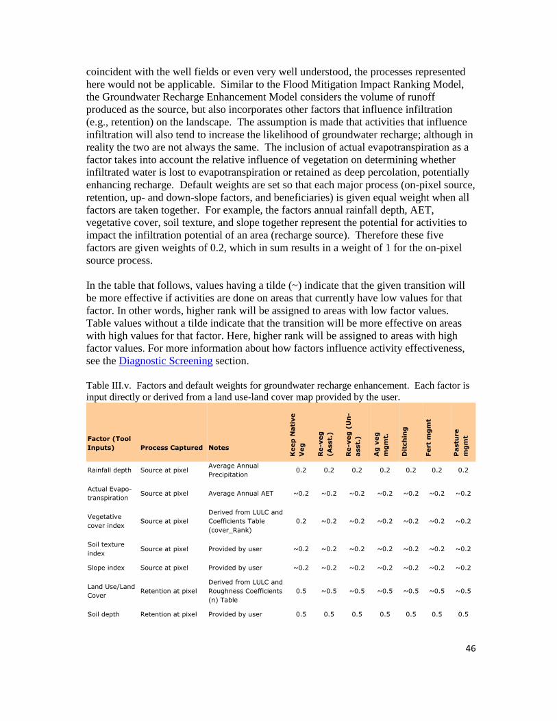
46

coincident with the well fields or even very well understood, the processes represented

here would not be applicable. Similar to the Flood Mitigation Impact Ranking Model,

the Groundwater Recharge Enhancement Model considers the volume of runoff

produced as the source, but also incorporates other factors that influence infiltration

(e.g., retention) on the landscape. The assumption is made that activities that influence

infiltration will also tend to increase the likelihood of groundwater recharge; although in

reality the two are not always the same. The inclusion of actual evapotranspiration as a

factor takes into account the relative influence of vegetation on determining whether

infiltrated water is lost to evapotranspiration or retained as deep percolation, potentially

enhancing recharge. Default weights are set so that each major process (on-pixel source,

retention, up- and down-slope factors, and beneficiaries) is given equal weight when all

factors are taken together. For example, the factors annual rainfall depth, AET,

vegetative cover, soil texture, and slope together represent the potential for activities to

impact the infiltration potential of an area (recharge source). Therefore these five

factors are given weights of 0.2, which in sum results in a weight of 1 for the on-pixel

source process.








Table III.v. Factors and default weights for groundwater recharge enhancement. Each factor is

input directly or derived from a land use-land cover map provided by the user.

Factor (Tool


Keep

Nati

ve

Veg

Re-v

eg

(A

sst.

)

Re-v

eg

(U

n-

asst.

)

Ag

veg

mg

mt.

Dit

ch

ing

Fert

mg

mt

Pastu

re

mg

mt

Rainfall depth Source at pixel Average Annual

Precipitation 0.2 0.2 0.2 0.2 0.2 0.2 0.2

Actual Evapo-

transpiration Source at pixel Average Annual AET ~0.2 ~0.2 ~0.2 ~0.2 ~0.2 ~0.2 ~0.2

Vegetative

cover index Source at pixel


Coefficients Table

(cover_Rank)

0.2 ~0.2 ~0.2 ~0.2 ~0.2 ~0.2 ~0.2

Soil texture

index Source at pixel Provided by user ~0.2 ~0.2 ~0.2 ~0.2 ~0.2 ~0.2 ~0.2

Slope index Source at pixel Provided by user ~0.2 ~0.2 ~0.2 ~0.2 ~0.2 ~0.2 ~0.2

Land Use/Land

Cover Retention at pixel


Roughness Coefficients

(n) Table

0.5 ~0.5 ~0.5 ~0.5 ~0.5 ~0.5 ~0.5

Soil depth Retention at pixel Provided by user 0.5 0.5 0.5 0.5 0.5 0.5 0.5

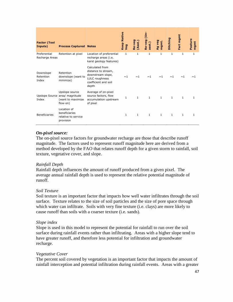
47

Factor (Tool


Keep

Nati

ve

Veg

Re-v

eg

(A

sst.

)

Re-v

eg

(U

n-

asst.

)

Ag

veg

mg

mt.

Dit

ch

ing

Fert

mg

mt

Pastu

re

mg

mt

Preferential

Recharge Areas

Retention at pixel Location of preferential

recharge areas (i.e.

karst geology features)

1 1 1 1 1 1 1

Downslope

Retention

Index

Retention

downslope (want to

minimize)

Calculated from

distance to stream,

downstream slope,

LULC roughness

coefficient and soil

depth

~1 ~1 ~1 ~1 ~1 ~1 ~1

Upslope Source

Index

Upslope source

area/ magnitude

(want to maximize

flow-on)

Average of on-pixel

source factors, flow


of pixel

1 1 1 1 1 1 1

Beneficiaries

Location of

beneficiaries

relative to service

provision

1 1 1 1 1 1 1

On-pixel source:

The on-pixel source factors for groundwater recharge are those that describe runoff

magnitude. The factors used to represent runoff magnitude here are derived from a

method developed by the FAO that relates runoff depth for a given storm to rainfall, soil

texture, vegetative cover, and slope.

Rainfall Depth

Rainfall depth influences the amount of runoff produced from a given pixel. The

average annual rainfall depth is used to represent the relative potential magnitude of

runoff.

Soil Texture





Slope index



have greater runoff, and therefore less potential for infiltration and groundwater

recharge.

Vegetative Cover



48



Mean Annual Actual Evapotranspiration (AET)

Actual evapotranspiration is influenced by vegetation and climate, and represents the

total amount of water lost from a natural system during an average year. Areas with

higher mean AET will have less water available for groundwater recharge or for

baseflow enhancement.

On-pixel retention:




travels across the surface as overland flow, and so is used here as a proxy for on-pixel

retention.

Soil depth

For groundwater recharge enhancement, the primary impact of soil depth is to enhance

potential infiltration and reduce runoff. Areas with higher soil depth tend to retain soil

water for a longer time following rainfall events than shallow soils, allowing more time

for water to percolate deeper and potentially recharge groundwater sources.

Preferential Recharge Areas

A large proportion of groundwater recharge can occur as water is precipitated onto, or

flows over, aquifers with prominent recharge features. This is especially true in areas of

significant karst development. Therefore activities to enhance recharge are most

effective if performed in areas where high potential for recharge exists based on an

assessment of the underlying geology.






the roughness (n) coefficient as weights. However, enhancing infiltration in close

proximity to a stream channel is unlikely to contribute to aquifer levels; rather the flow

will tend to travel quickly through the subsurface and emerge as baseflow to the stream.

A threshold value of 250 meters is used in RIOS, within which distance pixels are not

weighted highly for their influence on groundwater recharge.



a pixel. Because activities to enhance groundwater recharge will be most effective if

performed in an area with a large upslope runoff source (particularly if the receiving

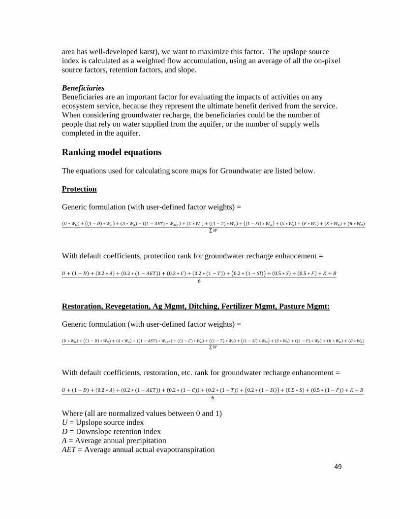
49

area has well-developed karst), we want to maximize this factor. The upslope source

index is calculated as a weighted flow accumulation, using an average of all the on-pixel

source factors, retention factors, and slope.

Beneficiaries



When considering groundwater recharge, the beneficiaries could be the number of

people that rely on water supplied from the aquifer, or the number of supply wells

completed in the aquifer.


The equations used for calculating score maps for Groundwater are listed below.

Protection


(𝑈 ∗ 𝑊𝑈) + ((1 − 𝐷) ∗ 𝑊𝐷) + (𝐴 ∗ 𝑊𝐴) + ((1 − 𝐴𝐸𝑇) ∗ 𝑊𝐴𝐸𝑇) + (𝐶 ∗ 𝑊𝐶) + ((1 − 𝑇) ∗ 𝑊𝑇) + ((1 − 𝑆𝑙) ∗ 𝑊𝑆𝑙) + (𝑆 ∗ 𝑊𝑆) + (𝐹 ∗ 𝑊𝐹) + (𝐾 ∗ 𝑊𝐾) + (𝐵 ∗ 𝑊𝐵)

∑ 𝑊

With default coefficients, protection rank for groundwater recharge enhancement = 𝑈 + (1 − 𝐷) + (0.2 ∗ 𝐴) + (0.2 ∗ (1 − 𝐴𝐸𝑇)) + (0.2 ∗ 𝐶) + (0.2 ∗ (1 − 𝑇)) + (0.2 ∗ (1 − 𝑆𝑙)) + (0.5 ∗ 𝑆) + (0.5 ∗ 𝐹) + 𝐾 + 𝐵

6


Generic formulation (with user-defined factor weights) = (𝑈 ∗ 𝑊𝑈) + ((1 − 𝐷) ∗ 𝑊𝐷) + (𝐴 ∗ 𝑊𝐴) + ((1 − 𝐴𝐸𝑇) ∗ 𝑊𝐴𝐸𝑇) + ((1 − 𝐶) ∗ 𝑊𝐶) + ((1 − 𝑇) ∗ 𝑊𝑇) + ((1 − 𝑆𝑙) ∗ 𝑊𝑆𝑙) + (𝑆 ∗ 𝑊𝑆) + ((1 − 𝐹) ∗ 𝑊𝐹) + (𝐾 ∗ 𝑊𝐾) + (𝐵 ∗ 𝑊𝐵)

∑ 𝑊

With default coefficients, restoration, etc. rank for groundwater recharge enhancement = 𝑈 + (1 − 𝐷) + (0.2 ∗ 𝐴) + (0.2 ∗ (1 − 𝐴𝐸𝑇)) + (0.2 ∗ (1 − 𝐶)) + (0.2 ∗ (1 − 𝑇)) + (0.2 ∗ (1 − 𝑆𝑙)) + (0.5 ∗ 𝑆) + (0.5 ∗ (1 − 𝐹)) + 𝐾 + 𝐵

6




A = Average annual precipitation

AET = Average annual actual evapotranspiration

50



Sl = Slope index

S = Soil depth

K = Preferential recharge index

F = Vegetation roughness coefficient






cell.



𝑊𝑥 =𝐴𝑥 + (1 − 𝐴𝐸𝑇𝑥) + (1 − 𝐶𝑥) + 𝑇𝑥 + 𝑆𝑙𝑥 + 𝑆𝑥 + (1 − 𝑅𝑒𝑡𝑥)

7

Where



Ax = Average annual precipitation (normalized values between 0 and 1)

AETx = Average annual actual evapotranspiration (normalized values between 0 and 1)





Fx = Vegetation roughness coefficient (normalized values between 0 and 1)







𝑊𝑥 =(1 − 𝑆𝑙𝑥) + 𝐹𝑥

2

Where



51




vi. Dry Season Baseflow

Vegetation can intercept rainfall, slow overland flow of water, and increase temporary

storage of subsurface water in soils, floodplains, and streambanks, which is later

released slowly during the dry season to increase the magnitude and permanence of low

flows. The primary factors derived from the literature review that influence seasonal

baseflow and the impact of activities to enhance it are given in Table III.vi and briefly

described below. Similar to the Flood Mitigation Impact and Groundwater Recharge

Enhancement Models, the Dry Season Baseflow Model considers the volume of runoff

produced as the source, but also incorporates other factors that influence infiltration

(e.g., retention) on the landscape. The assumption is made that activities that influence

infiltration will also tend to increase retention of water in the soil profile and facilitate its

slow release into streams. Default weights are set so that each major process (on-pixel

source, retention, up- and down-slope factors, and beneficiaries) is given equal weight

when all factors are taken together. For example, the factors annual rainfall depth, AET,

vegetative cover, soil texture, and slope together represent the potential for activities to

impact the infiltration potential of an area (source of infiltrated waters). Therefore these

five factors are given weights of 0.2, which in sum results in a weight of 1 for the on-

pixel source process.








Table III.vi. Factors and default weights for Dry Season Baseflow. Each factor is input directly

or derived from a land use-land cover map provided by the user.

Factor (Tool

Inputs)

Process

Captured Notes

Keep

Nati

ve V

eg

Re-v

eg

(A

sst.

)

Re-v

eg

(U

n-a

sst.

)

Ag

veg

mg

mt.

Dit

ch

ing

Fert

iliz

er

mg

mt.

Pastu

re

mg

mt.

Rainfall depth Source at

pixel

Average Annual

Precipitation 0.2 0.2 0.2 0.2 0.2 0.2 0.2

Actual Evapo-

transpiration

Source at

pixel Average Annual AET ~0.2 ~0.2 ~0.2 ~0.2 ~0.2 ~0.2 ~0.2

Vegetative cover

index

Source at

pixel

Derived from LULC

and Coefficients

Table (cover_Rank)

0.2 ~0.2 ~0.2 ~0.2 ~0.2 ~0.2 ~0.2

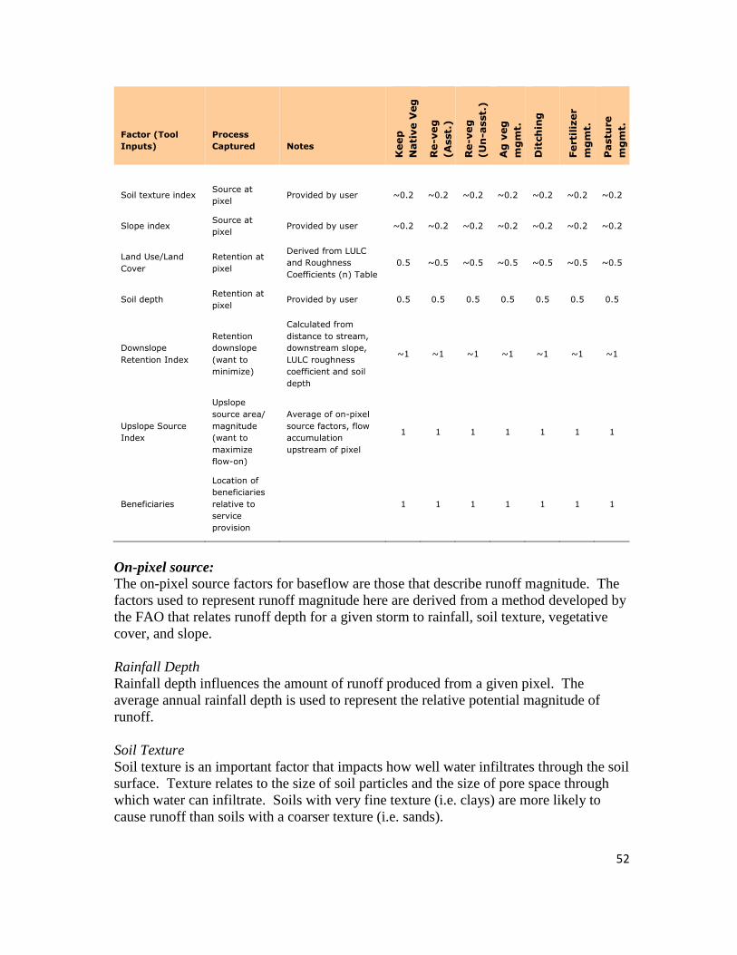
52

Factor (Tool

Inputs)

Process

Captured Notes

Keep

Nati

ve V

eg

Re-v

eg

(A

sst.

)

Re-v

eg

(U

n-a

sst.

)

Ag

veg

mg

mt.

Dit

ch

ing

Fert

iliz

er

mg

mt.

Pastu

re

mg

mt.

Soil texture index

Source at

pixel

Provided by user

~0.2

~0.2

~0.2

~0.2

~0.2

~0.2

~0.2

Slope index Source at

pixel Provided by user ~0.2 ~0.2 ~0.2 ~0.2 ~0.2 ~0.2 ~0.2

Land Use/Land

Cover

Retention at

pixel

Derived from LULC

and Roughness

Coefficients (n) Table

0.5 ~0.5 ~0.5 ~0.5 ~0.5 ~0.5 ~0.5

Soil depth Retention at

pixel Provided by user 0.5 0.5 0.5 0.5 0.5 0.5 0.5

Downslope

Retention Index

Retention

downslope

(want to

minimize)

Calculated from

distance to stream,

downstream slope,

LULC roughness

coefficient and soil

depth

~1 ~1 ~1 ~1 ~1 ~1 ~1

Upslope Source

Index

Upslope

source area/

magnitude

(want to

maximize

flow-on)

Average of on-pixel

source factors, flow

accumulation

upstream of pixel

1 1 1 1 1 1 1

Beneficiaries

Location of

beneficiaries

relative to

service

provision

1 1 1 1 1 1 1

On-pixel source:

The on-pixel source factors for baseflow are those that describe runoff magnitude. The

factors used to represent runoff magnitude here are derived from a method developed by

the FAO that relates runoff depth for a given storm to rainfall, soil texture, vegetative

cover, and slope.

Rainfall Depth

Rainfall depth influences the amount of runoff produced from a given pixel. The

average annual rainfall depth is used to represent the relative potential magnitude of

runoff.

Soil Texture





53

Slope index



have greater runoff, and therefore less potential for infiltration and baseflow regulation.

Vegetative Cover





Mean Annual Actual Evapotranspiration (AET)

Actual evapotranspiration is influenced by vegetation and climate, and represents the

total amount of water lost from a natural system during an average year. Areas with

higher mean AET will have less water available for groundwater recharge or for

baseflow enhancement.

On-pixel retention:




travels across the surface as overland flow, and so is used here as a proxy for on-pixel

retention.

Soil depth

Just as with groundwater recharge enhancement, the primary impact of soil depth in this

model is to enhance potential infiltration and reduce runoff. Areas with higher soil

depth tend to retain soil water for a longer time following rainfall events than shallow

soils, allowing water to be released slowly into receiving streams.






the roughness (n) coefficient as weights.



a pixel. Because activities to enhance baseflow will be most effective if performed in an

area with a large upslope runoff source, we want to maximize this factor. The upslope

source index is calculated as a weighted flow accumulation, using an average of all the

on-pixel source factors, retention factors, and slope.

54

Beneficiaries



When considering baseflow, the beneficiaries could be the number of people that rely on

water for irrigation or domestic supply from streams during the dry season, or an index

of species that rely on environmental flows.


The equations used for calculating score maps for Baseflow are listed below.

Protection


(𝑈 ∗ 𝑊𝑈) + ((1 − 𝐷) ∗ 𝑊𝐷) + (𝐴 ∗ 𝑊𝐴) + ((1 − 𝐴𝐸𝑇) ∗ 𝑊𝐴𝐸𝑇) + (𝐶 ∗ 𝑊𝐶) + ((1 − 𝑇) ∗ 𝑊𝑇) + ((1 − 𝑆𝑙) ∗ 𝑊𝑆𝑙) + (𝑆 ∗ 𝑊𝑆) + (𝐹 ∗ 𝑊𝐹) + (𝐵 ∗ 𝑊𝐵)

∑ 𝑊

With default coefficients, protection rank for base flow enhancement = 𝑈 + (1 − 𝐷) + (0.2 ∗ 𝐴) + (0.2 ∗ (1 − 𝐴𝐸𝑇)) + (0.2 ∗ 𝐶) + (0.2 ∗ (1 − 𝑇)) + (0.2 ∗ (1 − 𝑆𝑙)) + (0.5 ∗ 𝑆) + (0.5 ∗ 𝐹) + 𝐵

5


Generic formulation (with user-defined factor weights) = (𝑈 ∗ 𝑊𝑈) + ((1 − 𝐷) ∗ 𝑊𝐷) + (𝐴 ∗ 𝑊𝐴) + ((1 − 𝐴𝐸𝑇) ∗ 𝑊𝐴𝐸𝑇) + ((1 − 𝐶) ∗ 𝑊𝐶 ) + ((1 − 𝑇) ∗ 𝑊𝑇) + ((1 − 𝑆𝑙) ∗ 𝑊𝑆𝑙) + (𝑆 ∗ 𝑊𝑆) + ((1 − 𝐹) ∗ 𝑊𝐹) + (𝐵 ∗ 𝑊𝐵)

∑ 𝑊

With default coefficients, restoration, etc. rank for base flow enhancement = 𝑈 + (1 − 𝐷) + (0.2 ∗ 𝐴) + (0.2 ∗ (1 − 𝐴𝐸𝑇)) + (0.2 ∗ (1 − 𝐶)) + (0.2 ∗ (1 − 𝑇)) + (0.2 ∗ (1 − 𝑆𝑙)) + (0.5 ∗ 𝑆) + (0.5 ∗ (1 − 𝐹)) + 𝐵

5




A = Average annual precipitation

AET = Average annual actual evapotranspiration



Sl = Slope index

55

S = Soil depth

F = Vegetation roughness coefficient






cell.



𝑊𝑥 =𝐴𝑥 + (1 − 𝐴𝐸𝑇𝑥) + (1 − 𝐶𝑥) + 𝑇𝑥 + 𝑆𝑙𝑥 + 𝑆𝑥 + (1 − 𝑅𝑒𝑡𝑥)

7

Where



Ax = Average annual precipitation (normalized values between 0 and 1)

AETx = Average annual actual evapotranspiration (normalized values between 0 and 1)












𝑊𝑥 =(1 − 𝑆𝑙𝑥) + 𝐹𝑥

2

Where






56

vii. Biodiversity

Biodiversity is included as an option for RIOS users that have data on the biodiversity

value of the study area and wish to include this objective in the portfolio design. RIOS

does not model biodiversity directly, but can use inputs to rank the landscape for

biodiversity value relative to the transitions and other objectives. This objective

includes three optional input factors: protection score, restoration score, and agricultural

management score. These options allow users the flexibility to score the landscape

according to which areas are high priority for biodiversity in their current state

(protection), are high priority for biodiversity restoration, are high priority for

implementing agricultural practices that can increase biodiversity, or all three. The

default weight for each of these factors is set at 1.

viii. Other

RIOS includes three optional “Other” objectives that give users the flexibility to use any

prioritization method that they choose while taking advantage of the multi-objective

optimization and budget allocation tools that RIOS provides. Each “other” objective

includes three optional input factors: protection score, restoration score, and agricultural

management score. This allows users the flexibility to score the landscape relative to

whether the areas are high priority for the other objective in their current state

(protection), are high priority for restoration, are high priority for implementing

agricultural practices to reach the objective, or all three. The default weight for each of

these factors is set at 1.

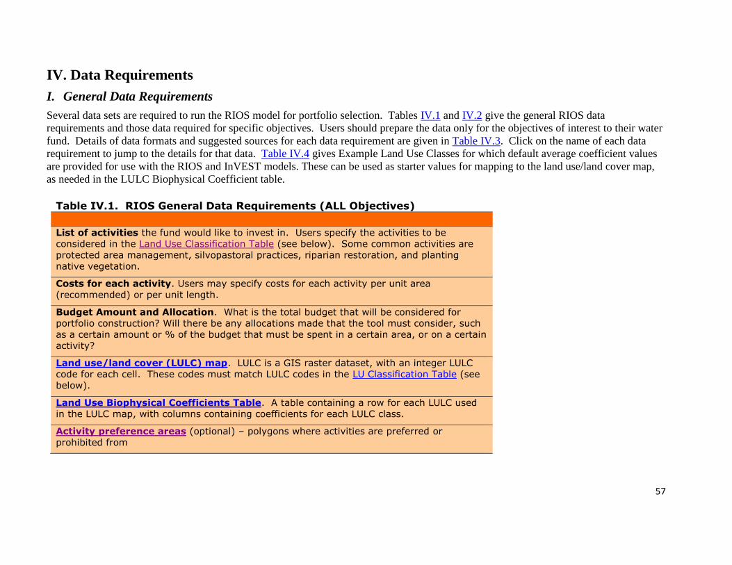
57

IV. Data Requirements

I. General Data Requirements

Several data sets are required to run the RIOS model for portfolio selection. Tables IV.1 and IV.2 give the general RIOS data

requirements and those data required for specific objectives. Users should prepare the data only for the objectives of interest to their water

fund. Details of data formats and suggested sources for each data requirement are given in Table IV.3. Click on the name of each data

requirement to jump to the details for that data. Table IV.4 gives Example Land Use Classes for which default average coefficient values

are provided for use with the RIOS and InVEST models. These can be used as starter values for mapping to the land use/land cover map,

as needed in the LULC Biophysical Coefficient table.

Table IV.1. RIOS General Data Requirements (ALL Objectives)

List of activities the fund would like to invest in. Users specify the activities to be

considered in the Land Use Classification Table (see below). Some common activities are

protected area management, silvopastoral practices, riparian restoration, and planting

native vegetation.

Costs for each activity. Users may specify costs for each activity per unit area

(recommended) or per unit length.

Budget Amount and Allocation. What is the total budget that will be considered for

portfolio construction? Will there be any allocations made that the tool must consider, such

as a certain amount or % of the budget that must be spent in a certain area, or on a certain

activity?

Land use/land cover (LULC) map. LULC is a GIS raster dataset, with an integer LULC

code for each cell. These codes must match LULC codes in the LU Classification Table (see

below).

Land Use Biophysical Coefficients Table. A table containing a row for each LULC used

in the LULC map, with columns containing coefficients for each LULC class.

Activity preference areas (optional) – polygons where activities are preferred or

prohibited from

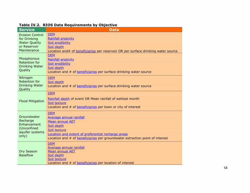
58

Table IV.2. RIOS Data Requirements by Objective

Service Data

Erosion Control

for Drinking

Water Quality

or Reservoir

Maintenance

DEM

Rainfall erosivity

Soil erodibility

Soil depth

Location and# of beneficiaries per reservoir OR per surface drinking water source

Phosphorous

Retention for

Drinking Water

Quality

DEM

Rainfall erosivity

Soil erodibility

Soil depth

Location and # of beneficiaries per surface drinking water source

Nitrogen

Retention for

Drinking Water

Quality

DEM

Soil depth

Location and # of beneficiaries per surface drinking water source

Flood Mitigation

DEM

Rainfall depth of event OR Mean rainfall of wettest month

Soil texture

Location and # of beneficiaries per town or city of interest

Groundwater

Recharge

Enhancement

(Unconfined

aquifer systems

only)

DEM

Average annual rainfall

Mean annual AET

Soil depth

Soil texture

Location and extent of preferential recharge areas

Location and # of beneficiaries per groundwater extraction point of interest

Dry Season

Baseflow

DEM


Mean annual AET

Soil depth

Soil texture

Location and # of beneficiaries per location of interest

59

Table IV.3. Details and Sources for Required Data

Data Description Sources

DEM

A GIS raster dataset with an elevation value for each cell. Use the highest quality, finest resolution DEM that

is appropriate for your application. This will reduce the chances of there being sinks and missing data, and will more accurately represent the terrain’s surface water flow, providing the amount of detail that is required for making informed decisions at your scale of interest.

Make sure the DEM is corrected by filling in sinks, and if necessary 'burning' hydrographic features into the

elevation model (recommended when you see unusual streams.) The same DEM may be used for all RIOS models and the InVEST sediment model.

DEM data is available for any area of the world, although at varying resolutions. Free raw global DEM data is available on the

internet from the USGS and World Wildlife Fund - http://hydrosheds.cr.usgs.gov/index.php. NASA provides free global 30m DEM data at http://asterweb.jpl.nasa.gov/gdem.asp as does the USGS -

http://eros.usgs.gov/#/Find_Data/Products_and_Data_Available/Elevation_Products. Or, it may be purchased relatively

inexpensively at sites such as MapMart.

Rainfall

erosivity

A GIS raster dataset, with an erosivity index value for each cell. This variable depends on the intensity and duration of rainfall in the area of interest. The greater

the intensity and duration of the rain storm, the higher the erosion potential. The same dataset may be used for all the sediment and nutrient models.

The erosivity index is widely used, but in case of its absence, there are methods and equations to help

generate a grid using climatic data. R should be obtained from published values, as calculation is very tedious. For calculation, R equals E (the kinetic energy of rainfall) times I30 (maximum intensity of rain in 30 minutes in cm/hr). Roose (1996) found that for Western Africa R = a * precipitation where a = 0.5 in most cases, 0.6 near the sea, 0.3 to 0.2 in tropical mountain

areas, and 0.1 in Mediterranean mountain areas.

The following equation is widely used to calculate the R index (http://www.fao.org/docrep/t1765e/t1765e0e.htm): R = E * I30 = (210 + 89log10I30)*I30

E: kinetic energy of rainfall expressed in metric MJ *

In the United States, national maps of the erosivity index can be found through the United States Department of Agriculture (USDA) and Environmental Protection Agency (EPA) websites.

The USDA published a loss handbook (http://www.epa.gov/npdes/pubs/ruslech2.pdf) that contains a hard copy map of the erosivity index for each region. Using

these maps requires creating a new line feature class in GIS and converting to raster. Please note that conversion of units is also required (multiply by 17.02).

The EPA has created a digital map that is available at http://www.epa.gov/esd/land-sci/emap_west_browser/pages/wemap_mm_sl_rusle_r_qt.htm. The map is in a shapefile format that needs to be converted to raster, along with an adjustment in units.

http://hydrosheds.cr.usgs.gov/index.php

http://asterweb.jpl.nasa.gov/gdem.asp

http://eros.usgs.gov/#/Find_Data/Products_and_Data_Available/Elevation_Products

http://eros.usgs.gov/#/Find_Data/Products_and_Data_Available/Elevation_Products

http://www.mapmart.com/

http://www.epa.gov/npdes/pubs/ruslech2.pdf

http://www.epa.gov/esd/land-sci/emap_west_browser/pages/wemap_mm_sl_rusle_r_qt.htm

http://www.epa.gov/esd/land-sci/emap_west_browser/pages/wemap_mm_sl_rusle_r_qt.htm

60


Data Description Sources m/ha/cm of rainfall. I30: maximum intensity of rain in 30 minutes expressed

in cm per hour.

61



Soil

erodibility

A GIS raster dataset, with a soil erodibility value for each cell. The same dataset may be used for all the

sediment and nutrient models. Soil erodibility, (sometimes noted as K), is a measure of the susceptibility of soil particles to detachment and transport by rainfall and runoff. Texture is the principal factor affecting K, but soil profile, organic matter and

permeability also contribute. It varies from 70/100 for the most fragile soil and 1/100 for the most stable soil. It is measured on bare reference plots 22.2 m long on 9% slopes, tilled in the direction of the slope and having received no organic matter for three years. Values of 0 – 0.6 are reasonable, while higher values should be given a critical look. K may be found as part of standard

soil data maps.

Coarse, yet free global soil characteristic data is available through NOAA's National Centers for Environmental Information

(NCEI). The FAO also provides global soil data in their Harmonized World Soil Database. In the United States free soil data is available from the U.S. Department of Agriculture’s NRCS in the form of two datasets: SSURGO and STATSGO. Where available, SSURGO data should

be used, as it is much more detailed than STATSGO. Where gaps occur in the SSURGO data, STATSGO can be used to fill in the blanks. The soil erodibility should be calculated as the average of all horizons within a soil class component, and then a weighted average of the components should be estimated. This can be a

tricky GIS analysis: In the US soil categories, each soil property polygon can contain a number of soil type components with unique properties, and each component may have different soil horizon layers, also with unique properties. Processing requires

careful weighting across components and horizons. The NRCS Soil Data Viewer, a free ArcMap extension from the NRCS, does this soil data processing for the user and should be used

whenever possible. The following equation can be used to calculate K (Wischmeier and Smith 1978):

𝐾

= 27.66 ∗ 𝑚1.14 ∗ 10−8 ∗ (12 − 𝑎) + (0.0043 ∗ (𝑏 − 2)) + (0.0033

∗ (𝑐 − 3)) In which K = soil erodibility factor (t ∗ ha/MJ ∗ mm)

m = (silt (%) + very fine sand (%))(100-clay (%)) a = organic matter (%) b = structure code: (1) very structured or particulate, (2) fairly structured, (3) slightly structured and (4) solid c = profile permeability code: (1) rapid, (2) moderate to rapid, (3) moderate, (4) moderate to slow, (5) slow and (6) very slow.

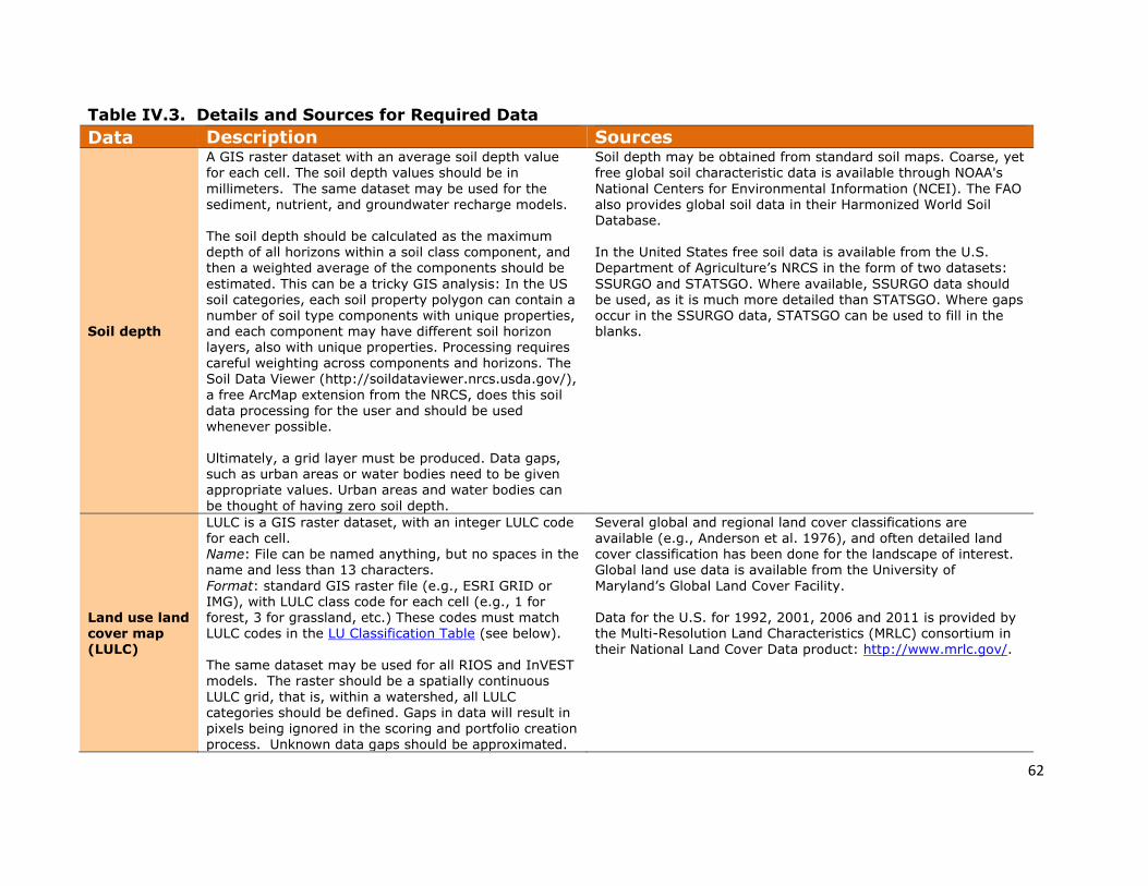
62



Soil depth

A GIS raster dataset with an average soil depth value for each cell. The soil depth values should be in

millimeters. The same dataset may be used for the sediment, nutrient, and groundwater recharge models. The soil depth should be calculated as the maximum depth of all horizons within a soil class component, and then a weighted average of the components should be

estimated. This can be a tricky GIS analysis: In the US soil categories, each soil property polygon can contain a number of soil type components with unique properties, and each component may have different soil horizon layers, also with unique properties. Processing requires careful weighting across components and horizons. The Soil Data Viewer (http://soildataviewer.nrcs.usda.gov/),

a free ArcMap extension from the NRCS, does this soil data processing for the user and should be used whenever possible.

Ultimately, a grid layer must be produced. Data gaps, such as urban areas or water bodies need to be given appropriate values. Urban areas and water bodies can

be thought of having zero soil depth.

Soil depth may be obtained from standard soil maps. Coarse, yet free global soil characteristic data is available through NOAA's

National Centers for Environmental Information (NCEI). The FAO also provides global soil data in their Harmonized World Soil Database. In the United States free soil data is available from the U.S. Department of Agriculture’s NRCS in the form of two datasets:

SSURGO and STATSGO. Where available, SSURGO data should be used, as it is much more detailed than STATSGO. Where gaps occur in the SSURGO data, STATSGO can be used to fill in the blanks.

Land use land cover map

(LULC)

LULC is a GIS raster dataset, with an integer LULC code for each cell. Name: File can be named anything, but no spaces in the name and less than 13 characters.

Format: standard GIS raster file (e.g., ESRI GRID or IMG), with LULC class code for each cell (e.g., 1 for forest, 3 for grassland, etc.) These codes must match LULC codes in the LU Classification Table (see below).

The same dataset may be used for all RIOS and InVEST models. The raster should be a spatially continuous

LULC grid, that is, within a watershed, all LULC categories should be defined. Gaps in data will result in pixels being ignored in the scoring and portfolio creation process. Unknown data gaps should be approximated.

Several global and regional land cover classifications are available (e.g., Anderson et al. 1976), and often detailed land cover classification has been done for the landscape of interest. Global land use data is available from the University of

Maryland’s Global Land Cover Facility. Data for the U.S. for 1992, 2001, 2006 and 2011 is provided by the Multi-Resolution Land Characteristics (MRLC) consortium in

their National Land Cover Data product: http://www.mrlc.gov/.

http://www.mrlc.gov/

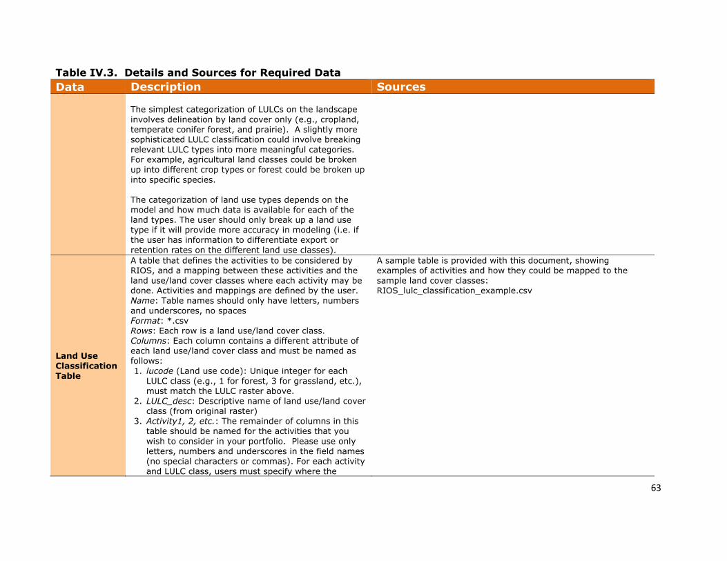
63


Data Description Sources The simplest categorization of LULCs on the landscape

involves delineation by land cover only (e.g., cropland, temperate conifer forest, and prairie). A slightly more sophisticated LULC classification could involve breaking relevant LULC types into more meaningful categories. For example, agricultural land classes could be broken up into different crop types or forest could be broken up

into specific species. The categorization of land use types depends on the model and how much data is available for each of the land types. The user should only break up a land use type if it will provide more accuracy in modeling (i.e. if the user has information to differentiate export or

retention rates on the different land use classes).

Land Use Classification Table

A table that defines the activities to be considered by RIOS, and a mapping between these activities and the land use/land cover classes where each activity may be

done. Activities and mappings are defined by the user. Name: Table names should only have letters, numbers

and underscores, no spaces Format: *.csv Rows: Each row is a land use/land cover class. Columns: Each column contains a different attribute of each land use/land cover class and must be named as follows:

1. lucode (Land use code): Unique integer for each LULC class (e.g., 1 for forest, 3 for grassland, etc.), must match the LULC raster above.

2. LULC_desc: Descriptive name of land use/land cover

class (from original raster) 3. Activity1, 2, etc.: The remainder of columns in this

table should be named for the activities that you

wish to consider in your portfolio. Please use only letters, numbers and underscores in the field names (no special characters or commas). For each activity and LULC class, users must specify where the

A sample table is provided with this document, showing examples of activities and how they could be mapped to the sample land cover classes:

RIOS_lulc_classification_example.csv

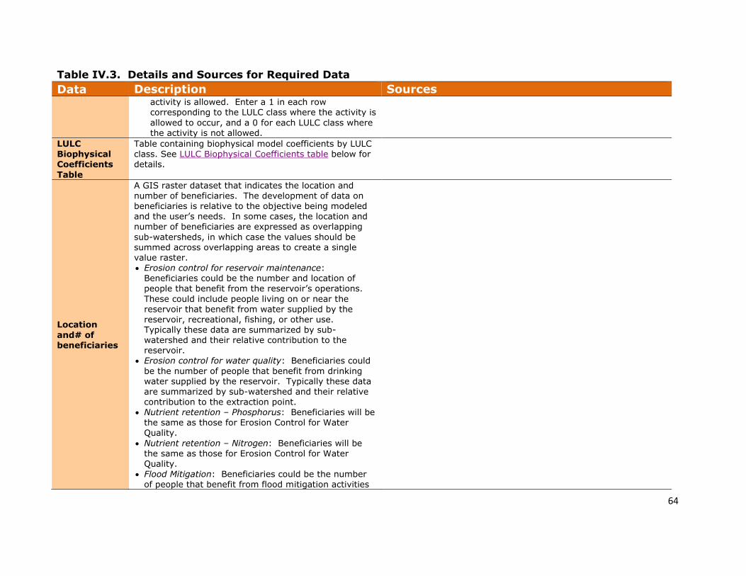
64


Data Description Sources activity is allowed. Enter a 1 in each row corresponding to the LULC class where the activity is

allowed to occur, and a 0 for each LULC class where the activity is not allowed.

LULC Biophysical Coefficients

Table

Table containing biophysical model coefficients by LULC class. See LULC Biophysical Coefficients table below for details.

Location

and# of beneficiaries

A GIS raster dataset that indicates the location and number of beneficiaries. The development of data on beneficiaries is relative to the objective being modeled and the user’s needs. In some cases, the location and number of beneficiaries are expressed as overlapping

sub-watersheds, in which case the values should be summed across overlapping areas to create a single value raster. Erosion control for reservoir maintenance:

Beneficiaries could be the number and location of people that benefit from the reservoir’s operations.

These could include people living on or near the reservoir that benefit from water supplied by the reservoir, recreational, fishing, or other use. Typically these data are summarized by sub-watershed and their relative contribution to the reservoir.

Erosion control for water quality: Beneficiaries could

be the number of people that benefit from drinking water supplied by the reservoir. Typically these data are summarized by sub-watershed and their relative contribution to the extraction point.

Nutrient retention – Phosphorus: Beneficiaries will be

the same as those for Erosion Control for Water Quality.

Nutrient retention – Nitrogen: Beneficiaries will be the same as those for Erosion Control for Water Quality.

Flood Mitigation: Beneficiaries could be the number of people that benefit from flood mitigation activities

65


Data Description Sources in the water fund area. This could be the population of a city that benefits from flood control, the

population of the likely flood-inundated area, or the value of infrastructure in a flood-inundated area. Typically these data would be summarized over the sub-watersheds that contribute flow to the area of interest.

Groundwater Recharge Enhancement: Beneficiaries

could be the number and location of people dependent on water supply from a given extraction point. Typically these data are summarized over the area likely to contribute to groundwater production at the extraction point.

Baseflow: Beneficiaries could be the number and location of people dependent on river flow for

domestic supply or crop irrigation during the dry season.

Rainfall depth

of event OR Mean rainfall of wettest month

This is a GIS raster dataset, with a value for rainfall depth for each cell in mm. Rainfall depth influences the

amount of runoff produced from a given pixel. This factor can be expressed as the average rainfall depth of

a given size storm that is likely to produce flooding (i.e. 10 year return period rainfall in mm). Often, these data are not available, so users can alternatively provide the mean rainfall of the wettest month (mm).

Mean rainfall of the wettest month is available globally at approximately 1 km resolution through the WorldClim Global

Climate Data product: http://worldclim.org/current

The mean rainfall of the wettest month is packaged with the BioClim variables (more information at http://worldclim.org/bioclim)

Soil texture

This is a GIS raster dataset, with an index (rank) value

for each cell that represents the soil texture class. The Soil Texture Index can be derived from a soils data layer, such as the FAO Harmonized World Soil Database. Each soil type must be assigned a rank, based on the texture:

Sandy 0.2 Light 0.4

Medium 0.6 Heavy 0.8 Heavy to Rock 1.0

Coarse, yet free global soil characteristic data is available

through NOAA's National Centers for Environmental Information (NCEI). The FAO also provides global soil data in their Harmonized World Soil Database. In the United States free soil data is available from the U.S.

Department of Agriculture’s NRCS in the form of two datasets: SSURGO and STATSGO. Where available, SSURGO data should

be used, as it is much more detailed than STATSGO. Where gaps occur in the SSURGO data, STATSGO can be used to fill in the blanks.


http://worldclim.org/bioclim

66


Data Description Sources The same dataset may be used for both the flood and groundwater recharge models.

The table below provides guidance for mapping commonly-used soil classes, including % sand-silt-clay to the classes and

coefficients shown at left (click here for a larger version).


This is a GIS raster dataset, with a value for mean annual rainfall depth for each cell in mm. Rainfall depth influences the amount of runoff produced from a given pixel. The average annual rainfall depth is used to represent the relative potential magnitude of runoff.

Mean annual rainfall is available globally at approximately 1 km resolution through the WorldClim Global Climate Data product.

Mean annual

Actual Evapo-transpiration (AET)

This is a GIS raster dataset, with a value for mean annual AET for each cell in mm. Actual evapotranspiration is important for groundwater

recharge, as areas with high AET are less likely to store water as groundwater recharge.

Mean annual AET is available globally at approximately 1 km resolution from CGIAR Consortium for Spatial Information, as part of the Global High-Resolution Soil-Water Balance product.

These data were modeled using the WorldClim and a global aridity and PET database as primary input. The method used to derive these datasets is described in the dataset documentation,

available online from CGIAR-CSI.

Location and extent of preferential recharge areas

A GIS raster dataset that indicates the presence or absence of preferential recharge areas for each pixel in the study area. In karst aquifers, a large proportion of recharge can occur as water is precipitated onto, or

flows over, areas with significant karst development. Therefore activities to enhance recharge are most effective if performed in areas with outcrops of karstic

geologic layers. For other unconfined aquifers, if hydrogeologic studies are available that identify areas of higher recharge, these could be used as inputs.

The location and extent of preferential recharge areas is often highly variable within a given study location. The protection/restoration of areas with a high degree of karst development, or other geologic features conducive to recharge,

can be very influential for determining the benefit of recharge enhancement activities. Because of the heterogeneous nature of karst geology and the importance of karst to groundwater

recharge, it is recommended that users obtain high-quality local data at the best possible resolution.

Watershed

A shapefile of polygons. This is a layer of watersheds such that each watershed contributes to a point of interest where the activity portfolio will be created. This

The watersheds layer should be derived from the same DEM used for modeling, to ensure that there are no inconsistencies between the two.

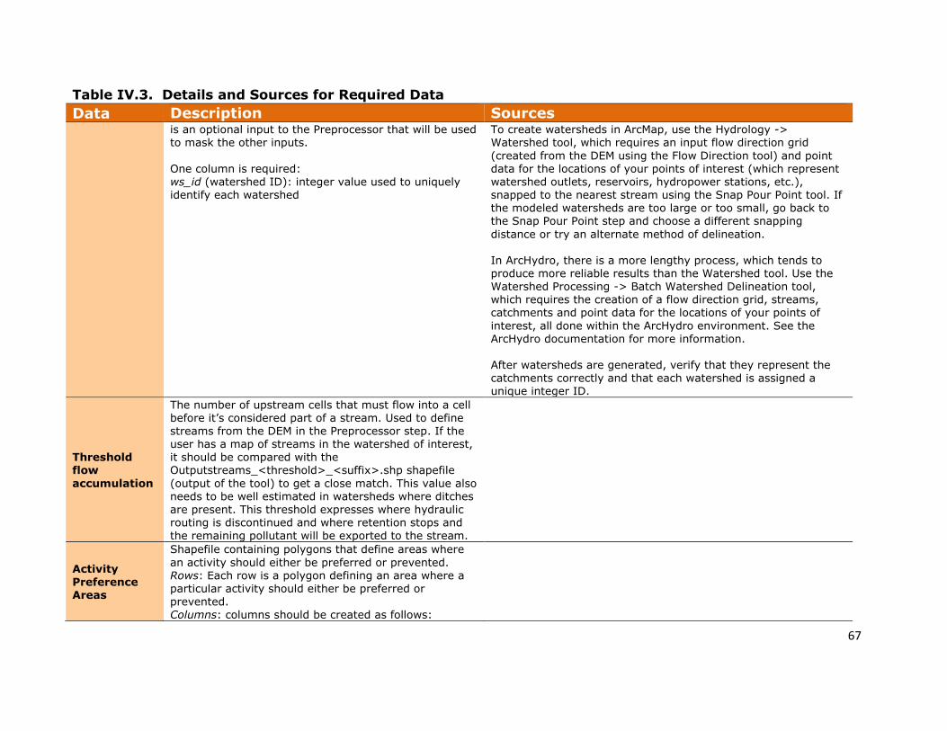
http://forum.naturalcapitalproject.org/uploads/FileUpload/d0/f11b65e36a6e0cce9b20a056f93df4.jpg


http://worldclim.org/

67


Data Description Sources is an optional input to the Preprocessor that will be used to mask the other inputs.

One column is required: ws_id (watershed ID): integer value used to uniquely identify each watershed

To create watersheds in ArcMap, use the Hydrology -> Watershed tool, which requires an input flow direction grid

(created from the DEM using the Flow Direction tool) and point data for the locations of your points of interest (which represent watershed outlets, reservoirs, hydropower stations, etc.), snapped to the nearest stream using the Snap Pour Point tool. If the modeled watersheds are too large or too small, go back to the Snap Pour Point step and choose a different snapping

distance or try an alternate method of delineation. In ArcHydro, there is a more lengthy process, which tends to produce more reliable results than the Watershed tool. Use the Watershed Processing -> Batch Watershed Delineation tool, which requires the creation of a flow direction grid, streams, catchments and point data for the locations of your points of

interest, all done within the ArcHydro environment. See the ArcHydro documentation for more information. After watersheds are generated, verify that they represent the

catchments correctly and that each watershed is assigned a unique integer ID.

Threshold flow

accumulation

The number of upstream cells that must flow into a cell before it’s considered part of a stream. Used to define streams from the DEM in the Preprocessor step. If the user has a map of streams in the watershed of interest, it should be compared with the Outputstreams_<threshold>_<suffix>.shp shapefile

(output of the tool) to get a close match. This value also needs to be well estimated in watersheds where ditches are present. This threshold expresses where hydraulic routing is discontinued and where retention stops and

the remaining pollutant will be exported to the stream.

Activity Preference Areas

Shapefile containing polygons that define areas where

an activity should either be preferred or prevented. Rows: Each row is a polygon defining an area where a particular activity should either be preferred or prevented. Columns: columns should be created as follows:

68


Data Description Sources 1. activity_n (activity name): Text value specifying

which activity is being preferred or prevented in

this polygon. Must match one of the activities defined in the LULC Classification CSV with Activities.

2. action: Text value specifying whether the activity is being preferred or prevented in this polygon. Valid values are ‘prefer’ and ‘prevent’.

The table below gives some example land use classes with RIOS coefficient values mapped to land cover types, as well as other

coefficients used by the SDR and water yield models, which are used by PORTER for generating input tables for InVEST. To use

these values, choose the example LULC class and values that best match your local LULC classification, and use the corresponding

coefficients given in the RIOS_default_LULC_coefficients.csv included with RIOS. Not all example land use classes will be present in

all regions. And please note that the values given in this table are global or regional averages, so they provide a good place to start,

but it is strongly recommended to do a literature search to refine these values for your area of interest. See LULC_Biophysical

Coefficients_table for more details.

Table IV.4. Land Use classes with default coefficients Land Use Class Description bare soil Areas characterized by bare rock, gravel, sand, silt, clay, or other earthen material, with

little or no "green" vegetation present.

open water All areas of open water, generally with less than 25% cover of vegetation or soil.

permanent crops Non-annual crops, i.e. rubber, oil palm, banana

temperate mixed forest Mix of evergreen, deciduous, or unspecified forest types in temperate regions. Neither deciduous nor evergreen species are greater than 75 percent of total tree cover.

tropical/subtropical mixed forest Mix of evergreen, deciduous, or unspecified forest types in tropical regions. Neither deciduous nor evergreen species are greater than 75 percent of total tree cover.

tropical montane/rain forest High elevation rain forest, cloud forest, or similar.

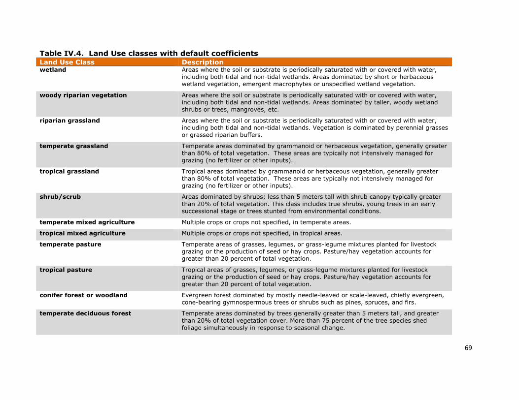
69

Table IV.4. Land Use classes with default coefficients Land Use Class Description wetland Areas where the soil or substrate is periodically saturated with or covered with water,

including both tidal and non-tidal wetlands. Areas dominated by short or herbaceous wetland vegetation, emergent macrophytes or unspecified wetland vegetation.

woody riparian vegetation Areas where the soil or substrate is periodically saturated with or covered with water, including both tidal and non-tidal wetlands. Areas dominated by taller, woody wetland shrubs or trees, mangroves, etc.

riparian grassland Areas where the soil or substrate is periodically saturated with or covered with water,

including both tidal and non-tidal wetlands. Vegetation is dominated by perennial grasses or grassed riparian buffers.

temperate grassland Temperate areas dominated by grammanoid or herbaceous vegetation, generally greater than 80% of total vegetation. These areas are typically not intensively managed for grazing (no fertilizer or other inputs).

tropical grassland Tropical areas dominated by grammanoid or herbaceous vegetation, generally greater than 80% of total vegetation. These areas are typically not intensively managed for grazing (no fertilizer or other inputs).

shrub/scrub Areas dominated by shrubs; less than 5 meters tall with shrub canopy typically greater

than 20% of total vegetation. This class includes true shrubs, young trees in an early

successional stage or trees stunted from environmental conditions.

temperate mixed agriculture Multiple crops or crops not specified, in temperate areas.

tropical mixed agriculture Multiple crops or crops not specified, in tropical areas.

temperate pasture Temperate areas of grasses, legumes, or grass-legume mixtures planted for livestock grazing or the production of seed or hay crops. Pasture/hay vegetation accounts for greater than 20 percent of total vegetation.

tropical pasture Tropical areas of grasses, legumes, or grass-legume mixtures planted for livestock grazing or the production of seed or hay crops. Pasture/hay vegetation accounts for greater than 20 percent of total vegetation.

conifer forest or woodland Evergreen forest dominated by mostly needle-leaved or scale-leaved, chiefly evergreen, cone-bearing gymnospermous trees or shrubs such as pines, spruces, and firs.

temperate deciduous forest Temperate areas dominated by trees generally greater than 5 meters tall, and greater

than 20% of total vegetation cover. More than 75 percent of the tree species shed foliage simultaneously in response to seasonal change.

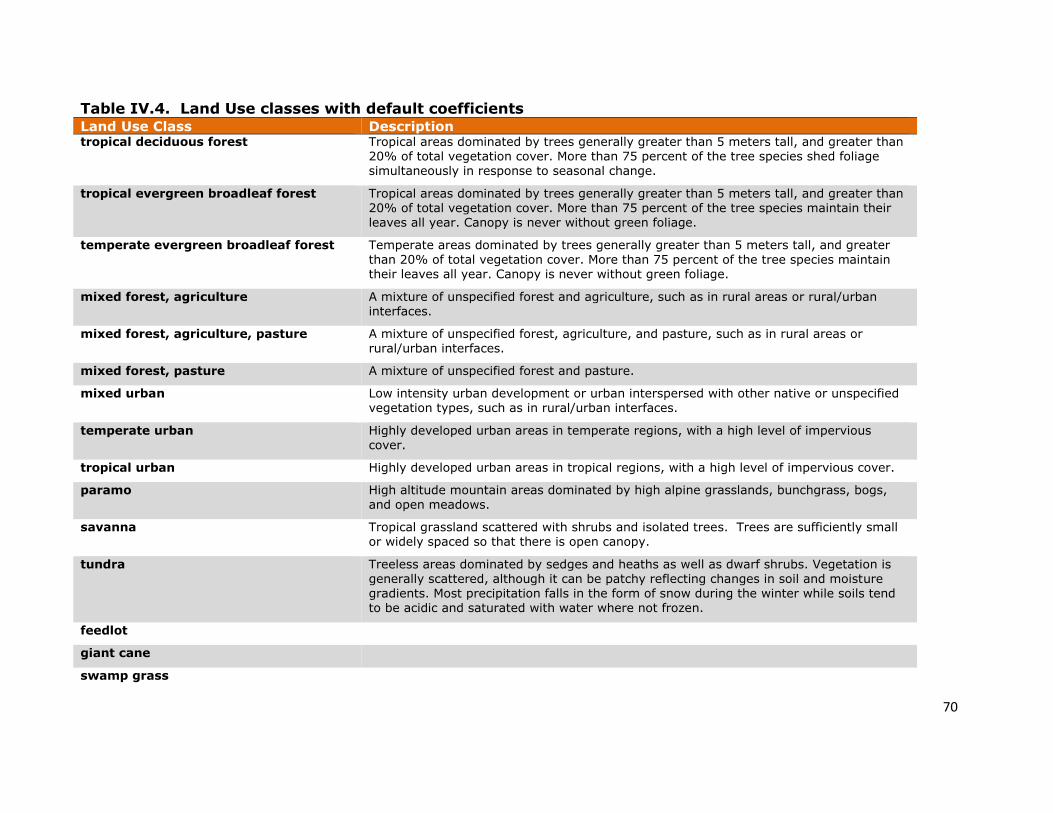
70

Table IV.4. Land Use classes with default coefficients Land Use Class Description tropical deciduous forest Tropical areas dominated by trees generally greater than 5 meters tall, and greater than

20% of total vegetation cover. More than 75 percent of the tree species shed foliage simultaneously in response to seasonal change.

tropical evergreen broadleaf forest Tropical areas dominated by trees generally greater than 5 meters tall, and greater than 20% of total vegetation cover. More than 75 percent of the tree species maintain their leaves all year. Canopy is never without green foliage.

temperate evergreen broadleaf forest Temperate areas dominated by trees generally greater than 5 meters tall, and greater

than 20% of total vegetation cover. More than 75 percent of the tree species maintain their leaves all year. Canopy is never without green foliage.

mixed forest, agriculture A mixture of unspecified forest and agriculture, such as in rural areas or rural/urban interfaces.

mixed forest, agriculture, pasture A mixture of unspecified forest, agriculture, and pasture, such as in rural areas or rural/urban interfaces.

mixed forest, pasture A mixture of unspecified forest and pasture.

mixed urban Low intensity urban development or urban interspersed with other native or unspecified vegetation types, such as in rural/urban interfaces.

temperate urban Highly developed urban areas in temperate regions, with a high level of impervious cover.

tropical urban Highly developed urban areas in tropical regions, with a high level of impervious cover.

paramo High altitude mountain areas dominated by high alpine grasslands, bunchgrass, bogs, and open meadows.

savanna Tropical grassland scattered with shrubs and isolated trees. Trees are sufficiently small or widely spaced so that there is open canopy.

tundra Treeless areas dominated by sedges and heaths as well as dwarf shrubs. Vegetation is generally scattered, although it can be patchy reflecting changes in soil and moisture

gradients. Most precipitation falls in the form of snow during the winter while soils tend to be acidic and saturated with water where not frozen.

feedlot

giant cane

swamp grass

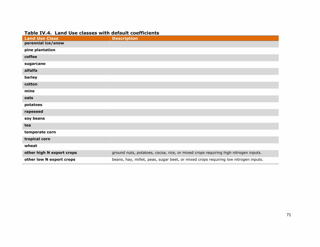
71

Table IV.4. Land Use classes with default coefficients Land Use Class Description perennial ice/snow

pine plantation

coffee

sugarcane

alfalfa

barley

cotton

mine

oats

potatoes

rapeseed

soy beans

tea

temperate corn

tropical corn

wheat

other high N export crops ground nuts, potatoes, cocoa, rice, or mixed crops requiring high nitrogen inputs.

other low N export crops beans, hay, millet, peas, sugar beet, or mixed crops requiring low nitrogen inputs.

72

ii. Required Data Pre-Processing

Several of the input data required by RIOS require some pre-processing from raw data

before they are used in the Investment Portfolio Advisor module. For example, the

upslope source index is calculated as a weighted flow accumulation, taking into account

the export and retention factors from all pixels that contribute to each area. Users may

choose to perform the pre-processing steps in any GIS program of their choice.

Alternatively, the RIOS installation package includes a pre-processing toolbox,

compatible with ArcGIS10.x, that takes raw data and performs the necessary processing

steps to calculate the upslope source, downslope retention, riparian continuity and/or

slope indices required by RIOS.

The ArcGIS pre-processing toolbox can be found in the RIOS install folder. Once the

RIOS program is installed, you can load the toolbox into ArcGIS. To run the pro-

processing tool, open ArcGIS and the ArcToolbox window. In the ArcToolbox window,

right click on ArcToolbox, and choose “Add Toolbox.” Navigate to the RIOS program

directory and locate the pre-processing toolbox. For a Windows machine, this is

typically C:\Program Files\RIOS <version>\RIOS_Pre_Processing.tbx. The toolbox will

be loaded into ArcGIS. Double click on the RIOS Pre-Processing toolbox to launch the

tool. Make sure that the tool Help is shown in the right hand side of the input window (if

it’s not, click the Show Help button at the bottom of the screen.) This contains useful

information about which inputs are required for each selected objective. When the tool is

launched, most of the inputs will be labeled as ‘optional’, even though some of them will

be required, depending on which objectives are selected. Choose the objectives for which

you need to process data, and provide the necessary data inputs. Click OK to run the

program.

When complete, the tool will create a folder within your specified workspace called

“Output.” Within this directory, you will find the upslope source, downslope retention,

riparian continuity and/or slope indices data sets that RIOS requires. Each output is

labeled with the objective name for which it applies and the user-designated suffix, for

example “erosion_downslope_retention_index_1.tif.”

It is not necessary to use the pre-processing tool in ArcGIS to prepare these data layers.

Any GIS program that has similar processing tools may be used instead. Step-by-step

instructions for calculating these inputs outside of ArcGIS are available on request.

Please visit the User Forum to send us a message requesting these instructions.

iii. Default LULC Data Provided with RIOS

LULC Biophysical Coefficients Table

RIOS requires a table of coefficients that represent parameters such as export, retention,

vegetation cover, etc. which map to each land use/land cover class in the LULC raster.

These coefficients are used in the impact ranking models to determine the relative impact

of different transitions on different land cover types. Generally, these coefficients are

http://forum.naturalcapitalproject.org/

73

obtained through a literature search, to find values that best represent the land cover

classes, practices and conditions in your area of interest. Since this can be a lengthy

process, RIOS provides a table of default biophysical coefficient values for a selection of

land cover classes, which may be used as a starting point. The table is called

RIOS_default_lulc_coefficients.csv, and the list of selected LULC classes is listed in

Table IV.4. To use these values, look for the LULC class that most closely corresponds to

each LULC class in your LULC raster, and copy these values into your LULC

Biophysical Coefficients CSV table (format described below).

The default values provided with RIOS were derived from a review of the InVEST

sediment and nutrient model parameters database

(http://naturalcapitalproject.org/database.html) along with other relevant literature. Since

RIOS was originally developed for Latin America, these default values represent

averages for Latin America or, in some cases, global averages. It is strongly

recommended that users do a literature search, talk to local agencies, etc. to modify the

values from this table, in order to get more relevant and location-specific coefficients.

The format of this file should be as follows:

Name: Table names should only have letters, numbers and underscores. No spaces or

special characters.

Format: *.csv (Comma Separated Value table)

Rows: Each row is a land use/land cover class.

Columns: All column headers (with listed field names) must be present in the table. Each

column contains a different attribute of each land use/land cover class and must be named

as follows. Note that RIOS will allow missing (null) values in the table for objectives

that are not selected during the model run. If any values are missing for selected

objectives, users will see an error.

1. description: Text description of the LULC class.

2. lucode: Unique integer value corresponding to the LULC class values in the input

LULC raster.

3. native_veg: This integer field specifies whether the LULC class is a native

(unconverted) vegetation class or not. This field is used to determine the ending

point for restoration or revegetation activities. Since the objective of restoration

is to restore natural or unconverted land types, then only those classes assigned a

“1” in this field will be considered as potential end-points for restoration

activities. Values should be entered as follows:

0 = converted (i.e. pasture, cropland, urban)

1 = unconverted/native (i.e. forest, grassland, wetland)

4. sed_exp: For calculation of the upstream contributing source for each pixel, we

need a simple way to represent the ability of each LULC class to serve as an

erosion source. The Universal Soil Loss Equation uses the C factor, or crop factor,

http://naturalcapitalproject.org/database.html

74

to represent how susceptible each LULC type is to erosion. This is a decimal

value between 0 and 1. The default values were derived from a literature search

on USLE studies, using the mean of C factor values provided.

5. sed_ret: For calculating the ability for the landscape downstream of a pixel to

retain sediment, we need a simple way to reflect each LULC class’s retention

efficiency. The sed_ret coefficient is a decimal value from 0-1 that indicates what

portion of sediment that comes onto a pixel from upstream is retained by that

landcover type. Many studies have experimentally determined retention

efficiencies in buffer strips. Although buffers are not equivalent to continuous

vegetation on the landscape, there are very few studies that observe the latter. We

use observed average percent (in decimal form) retention efficiencies, determined

from a global literature review, to establish the relative ability of each LULC type

to retain sediment.

6. N_exp: For calculating the upstream contributing source for each pixel, we need a

simple way to represent the ability of each LULC class to serve as nitrogen

source. This parameter represents the average nitrogen loading for each land use.

The default values provided with RIOS are based on normalized median values

from our literature search, but users can also enter loading values from literature

with units of g Ha-1 yr-1, and the software will automatically normalize when

calculating the factor scores.

7. N_ret: For calculating the ability for the landscape downstream of a pixel to retain

nitrogen, we need a simple way to reflect each LULC class’s retention efficiency,

expressed as the fraction of nitrogen retained (between 0 and 1). Many studies

have experimentally determined retention efficiencies in buffer strips. Although

buffers are not equivalent to continuous vegetation on the landscape, there are

very few studies that observe the latter.

8. P_exp: For calculation of the upstream contributing source for each pixel, we

need a simple way to represent the ability of each LULC class to serve as a

phosphorus source. This parameter represents the average phosphorus loading for

each land use. The default values provided with RIOS are based on normalized

median values from our literature search, but users can also enter loading values

from literature with units of g Ha-1 yr-1, and the software will automatically

normalize when calculating the factor scores.

9. P_ret: For calculating the ability for the landscape downstream of a pixel to retain

phosphorus, we need a simple way to reflect each LULC class’s retention

efficiency, expressed as the fraction of phosphorus retained (between 0 and 1).

Many studies have experimentally determined retention efficiencies in buffer

strips. Although buffers are not equivalent to continuous vegetation on the

landscape, there are very few studies that observe the latter.

75

10. rough_rank: For calculating the ability for the landscape to retard flow, we need a

simple way to reflect each LULC class’s surface roughness. The default value in

RIOS is the normalized Manning’s n parameter for overland flow, which may be

found in a variety of literature sources.

11. cover_rank: For calculating the likelihood for a given land cover type to produce

runoff, we need a simple way to reflect each LULC class’s vegetative cover. This

parameter is the fraction of surface covered by vegetation, often reported as

percent cover. This is a value between 0 (no cover) and 1 (100% cover). One way

to calculate this (if field studies are not available) is using Leaf Area Index

information (calculated using remote sensing data) and taking an average over

each LULC class.

12. usle_c: This factor is used in the InVEST SDR model, and is the cover and

management factor for the USLE equation. This value is given as a floating point

number that ranges from 0.0 to 1.0. In most cases this will be identical to the

Sed_Exp column values. RIOS uses usle_c in the Portfolio Translator when

preparing inputs for InVEST. See the InVEST User Guide for details. Even if

InVEST will not be run, this column header must still be present.

13. usle_p: This factor is used in the InVEST SDR model, and is the management

practice factor for the USLE equation. This value is given as a floating point

number that ranges from 0.0 to 1.0. RIOS uses usle_p in the Portfolio Translator

when preparing inputs for InVEST. See the InVEST User Guide for details. Even

if InVEST will not be run, this column header must still be present.

14. root_depth: This factor is used in the InVEST Water Yield model, and is the

maximum root depth for vegetated land use classes, given in integer millimeters.

Non-vegetated LULCs should be given a value of 1. RIOS uses root_depth in the

Portfolio Translator when preparing inputs for InVEST. See the InVEST User

Guide for details. Even if InVEST will not be run, this column header must still

be present.

15. Kc: This factor is used in the InVEST Water Yield model, and is the

evapotranspiration coefficient for each LULC class, used to obtain actual

evapotranspiration by using plant energy/transpiration characteristics to modify

the reference evapotranspiration, which is based on alfalfa (or grass). Coefficients

should range between 0.01 and 1.5 (some crops evapotranspire more than alfalfa

in some very wet tropical regions and where water is always available). RIOS

uses Kc in the Portfolio Translator when preparing inputs for InVEST. See the

InVEST User Guide for details. Even if InVEST will not be run, this column

header must still be present.

16. LULC_veg: This factor is used in the InVEST Water Yield model, and is a 0 or 1

value indicating which Actual ET equation to use. Values should be 1 for

http://data.naturalcapitalandresilienceplatform.org/invest-releases/documentation/current_release/sdr.html

http://data.naturalcapitalandresilienceplatform.org/invest-releases/documentation/current_release/sdr.html

http://data.naturalcapitalandresilienceplatform.org/invest-releases/documentation/current_release/reservoirhydropowerproduction.html



76

vegetated land use except wetlands, and 0 for all other land uses, including

wetlands, urban, water bodies, etc. See the InVEST User Guide for details. Even

if InVEST will not be run, this column header must still be present.

Refer to RIOS_default_lulc_coefficients.csv provided with the latest RIOS installation

package for sample land use classes and default values. This file is found in the RIOS

sample data and in the program folder in the following location: C:\Program Files\RIOS

<version>\.


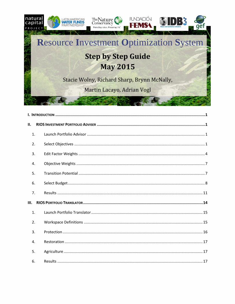
Resource Investment Optimization System

Step by Step Guide

May 2015

Stacie Wolny, Richard Sharp, Brynn McNally,

Martin Lacayo, Adrian Vogl

I. INTRODUCTION ..................................................................................................................................1

II. RIOS INVESTMENT PORTFOLIO ADVISER ..............................................................................................1

1. Launch Portfolio Advisor ............................................................................................................... 1

2. Select Objectives ........................................................................................................................... 1

3. Edit Factor Weights ....................................................................................................................... 4

4. Objective Weights ......................................................................................................................... 7

5. Transition Potential ....................................................................................................................... 7

6. Select Budget ................................................................................................................................. 8

7. Results ......................................................................................................................................... 11

III. RIOS PORTFOLIO TRANSLATOR ........................................................................................................ 14

1. Launch Portfolio Translator ......................................................................................................... 15

2. Workspace Definitions ................................................................................................................ 15

3. Protection .................................................................................................................................... 16

4. Restoration .................................................................................................................................. 17

5. Agriculture ................................................................................................................................... 17

6. Results ......................................................................................................................................... 17

1

I. Introduction This guide provides a basic orientation to RIOS software for first-time users. It provides an example

of a simple RIOS analysis and introduces the three modules that comprise the tool. For detailed

information on the theory of RIOS and support on more advanced analyses, see the full RIOS User’s

Guide.

A full RIOS analysis takes place over two modules:

RIOS Investment Portfolio Adviser

RIOS Portfolio Translator

Outputs from the previous two steps may be used with the InVEST suite of models to estimate

ecosystem services benefits from the portfolio. Users are referred to the InVEST model

documentation for details on how to use those models to simulate changes in ecosystem service

delivery and value.

Below, we provide a step by step example of a basic run of the RIOS tool.

II. RIOS Investment Portfolio Adviser

1. Launch Portfolio Adviser

The Investment Portfolio Adviser module uses biophysical and social data, budget information,

and implementation costs to produce investment portfolios for a given watershed investment

area. Users will input information on the objectives of their investments, the restoration or

protection activities they are considering, the costs of those activities and feasible locations to

undertake them, and the available budget for distributing funds among activities. The

investment portfolio that results provides a map indicating where investments in each activity

will yield the best return in terms of improvements across all ecosystem service objectives

selected. Launch the RIOS Investment Portfolio Adviser from the Windows Start menu. The

application will look similar to the following:

2. Select Objectives

Once launched, the main screen of the RIOS Investment Portfolio Adviser initially looks like this:

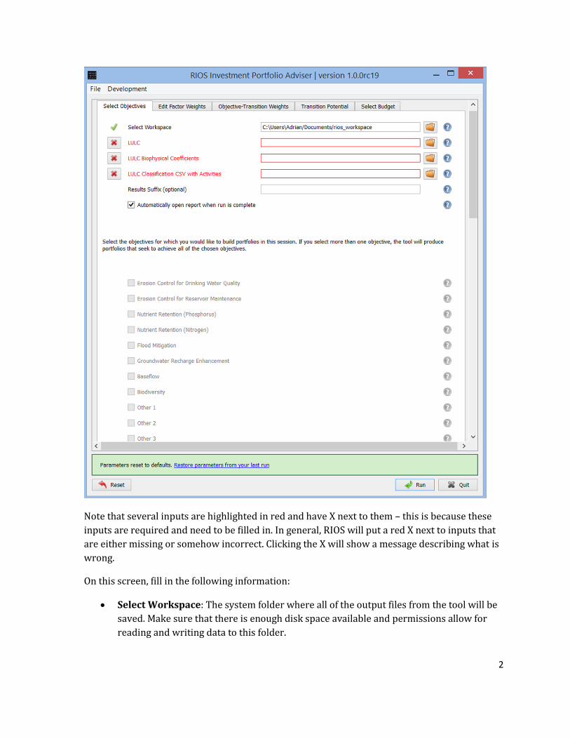
http://ncp-dev.stanford.edu/~dataportal/invest-releases/documentation/current_release/

http://ncp-dev.stanford.edu/~dataportal/invest-releases/documentation/current_release/

2

Note that several inputs are highlighted in red and have X next to them – this is because these

inputs are required and need to be filled in. In general, RIOS will put a red X next to inputs that

are either missing or somehow incorrect. Clicking the X will show a message describing what is

wrong.

On this screen, fill in the following information:

Select Workspace: The system folder where all of the output files from the tool will be

saved. Make sure that there is enough disk space available and permissions allow for

reading and writing data to this folder.

3

LULC: Raster layer containing Land Use/Land Cover data, with a unique integer value

assigned to each LULC class.

LULC Biophysical Coefficients: Table in .csv (Comma Separated Value) format,

containing mappings from each LULC class in the LULC raster to model input

coefficients specific to each Objective. See the LULC Biophysical Coefficients section for

details on required fields and values for creating this table, as well as information on

default values provided with RIOS.

LULC Classification CSV with Activities: Table in .csv (Comma Separated Value)

format, containing mappings from each Land Use/Land Cover class in the LULC raster to

the activities that are allowed to occur on that class. See the Land Use Classification

Table data entry for details on the required fields and values.

Results Suffix: Optional text string that will be appended to the end of output

filenames, in the form of <Filename>_<Suffix>. This can be used to generate unique

output filenames distinguishing multiple scenarios or projects.

Automatically open report when run is complete: RIOS automatically opens an html

report (showing budgets and spending on activities) when processing is complete. By

unchecking the box, users can disable this function. Disabling automatic opening of

reports is recommended when running RIOS many times in batch mode.

Objectives: Put a check next to the ecosystem service objectives that should be evaluated. For more

information on objectives, see the Objectives section. For each objective selected, a set of input data

will be requested by the tool in the next step.

The screenshot below shows these inputs filled in with a non-default Workspace, and both LULC

and LULC Classification CSV with Activities set to data for a case study in the Willamette watershed.

Baseflow and Biodiversity have been selected as Objectives.

4

3. Edit Factor Weights

Next, select the “Edit factor weights” tab. Tabs corresponding to the objectives checked in the

“Select objectives” step will be active, with the rest in gray color. Select each of the active tabs

and fill in the required objective factors. Some of these factors are basic data layers (such as soil

depth and beneficiaries), while others are derivative layers produced by running the RIOS

Preprocessor. (The RIOS Preprocessor is an ArcGIS tool that assists in formatting biophysical

data for RIOS inputs, and is included with the RIOS download. See the Pre-Processing section

for details.)

5

The table at the top of the window defines weights assigned to each factor, based on how

important that factor is in influencing each transition type, relative to the other factors listed.

These values may be adjusted, based on the objective and specific context of a particular

project. For more information on objective factors and weights, see Section III, Description of

Models. For more information on the relationship between activities and transitions, see

Transitions and Activities.

The first example below shows the Baseflow factor tab, with the first two factors (Annual

Average Rainfall and Actual Evapotranspiration) filled in:

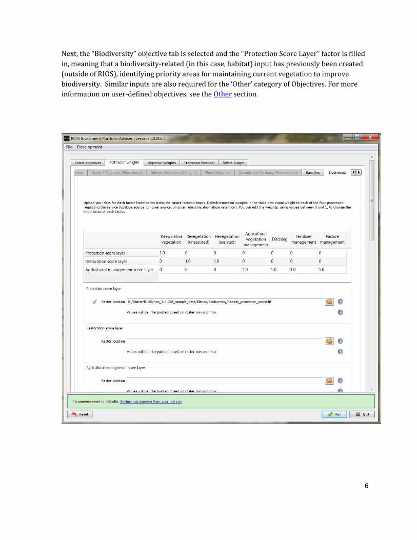
6

Next, the “Biodiversity” objective tab is selected and the “Protection Score Layer” factor is filled

in, meaning that a biodiversity-related (in this case, habitat) input has previously been created

(outside of RIOS), identifying priority areas for maintaining current vegetation to improve

biodiversity. Similar inputs are also required for the ‘Other’ category of Objectives. For more

information on user-defined objectives, see the Other section.

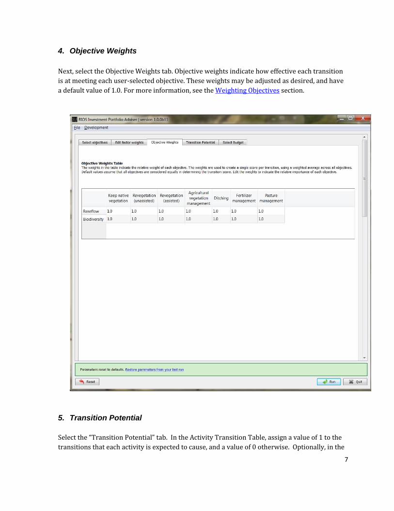
7

4. Objective Weights

Next, select the Objective Weights tab. Objective weights indicate how effective each transition

is at meeting each user-selected objective. These weights may be adjusted as desired, and have

a default value of 1.0. For more information, see the Weighting Objectives section.

5. Transition Potential

Select the “Transition Potential” tab. In the Activity Transition Table, assign a value of 1 to the

transitions that each activity is expected to cause, and a value of 0 otherwise. Optionally, in the

8

Activity Preferences section, click “Add another” to input shapefiles containing polygons that

define areas where an activity should either be preferred or prevented. For additional

information, see Activity Preference Areas for a general description and Table IV.3 for specifics

about the shapefile table format. In the example below the ‘protection’ activity can only cause

the ‘Keep native vegetation’ transition. The user has also added one activity preference

shapefile for the activity of ‘protection’

6. Select Budget

Finally, click on the “Select Budget” tab to fill out budget preferences and activity costs. For

more information, see the Budget Allocation section. Note that the type of currency used here

9

does not matter, as long as it is consistent across all entries of budget and cost. Enter the

following information:

Number of years: Integer value specifying how many years the analysis should be

performed for. If a value of 1 is entered, results will correspond to one year’s worth

of specified budget expenditure. If a value greater than 1 is entered, the specified

budget will be spent each year, and a separate portfolio will be created for each

year, as well as a combined portfolio containing recommended activities covering all

years. Note that investments are still chosen by cost-effectiveness, with the most

cost-effective activities that can be spent with a given year’s budget assigned to that

year. Therefore, applying number of years greater than one is a way to sort the

portfolios into bins of cost-effectiveness score.

If activity money cannot be spent: When using the Yearly Activity Allocation Table,

if more money is budgeted for an activity than can be spent, the surplus amount can

either simply be listed in the final HTML report and not spent (corresponding to

‘Report remainder’) or redistributed among other activities, based on the

proportion of the budget originally allocated to each activity (corresponding to

‘Proportionally reallocate’.)

Yearly floating budget: Floating point value specifying the amount of money that

should be spent on activities, based solely on return on investment. Note that only

allocating a floating budget (without specific amounts given to each activity in the

Yearly Activity Allocation Table) may lead to only the cheapest activities being

selected, thus not all activities may be represented in the final portfolio. Both Yearly

floating budget and Activity Allocation Table may be used at the same time.

Yearly Activity Allocation Table: Floating point values specifying the amount of

money that should be spent exclusively on each activity per year. Both Yearly

floating budget and Activity Allocation Table may be used at the same time.

Activity cost: Floating point values specifying how much each activity costs to

implement. Three pieces of information are required for each activity:

i. Cost per unit: Floating point value for the implementation cost per unit

area.

ii. Measurement unit: If the cost is given per unit of area, select ‘area’, if it is

given per unit of length, select ‘length’. Based on pixel size, RIOS converts

the cost entered above to a per-pixel cost for each activity in order to

calculate cost-effectiveness scores. If ‘length’ is chosen, RIOS uses the pixel

length to convert to per-pixel cost. We strongly recommend that users

choose area-based costs rather than length-based costs, unless the activity is

one that is likely to be implemented along one length of each pixel only.

iii. Length (m) or Area (m^2): Floating point value specifying the size of the

length (in meters) or unit of area (in square meters.)

10

For example, if an activity costs $100/hectare, enter ‘100’ for ‘Cost per unit’, ‘area’

for ‘Measurement unit’ and ’10000’ for ‘Length (m) or Area (m^2)’ (as there are

10000 square meters per hectare.)

In the example below the user has filled in 100,000 as a Floating Budget to spend in a

single year, allocated specific budgets to individual activities, and entered activity costs per

hectare (10000m^2).

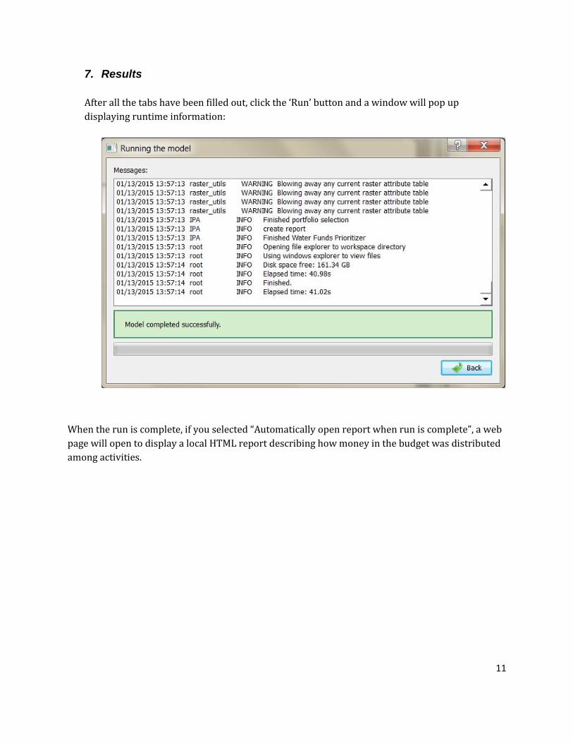
11

7. Results

After all the tabs have been filled out, click the ‘Run’ button and a window will pop up

displaying runtime information:

When the run is complete, if you selected “Automatically open report when run is complete”, a web

page will open to display a local HTML report describing how money in the budget was distributed

among activities.

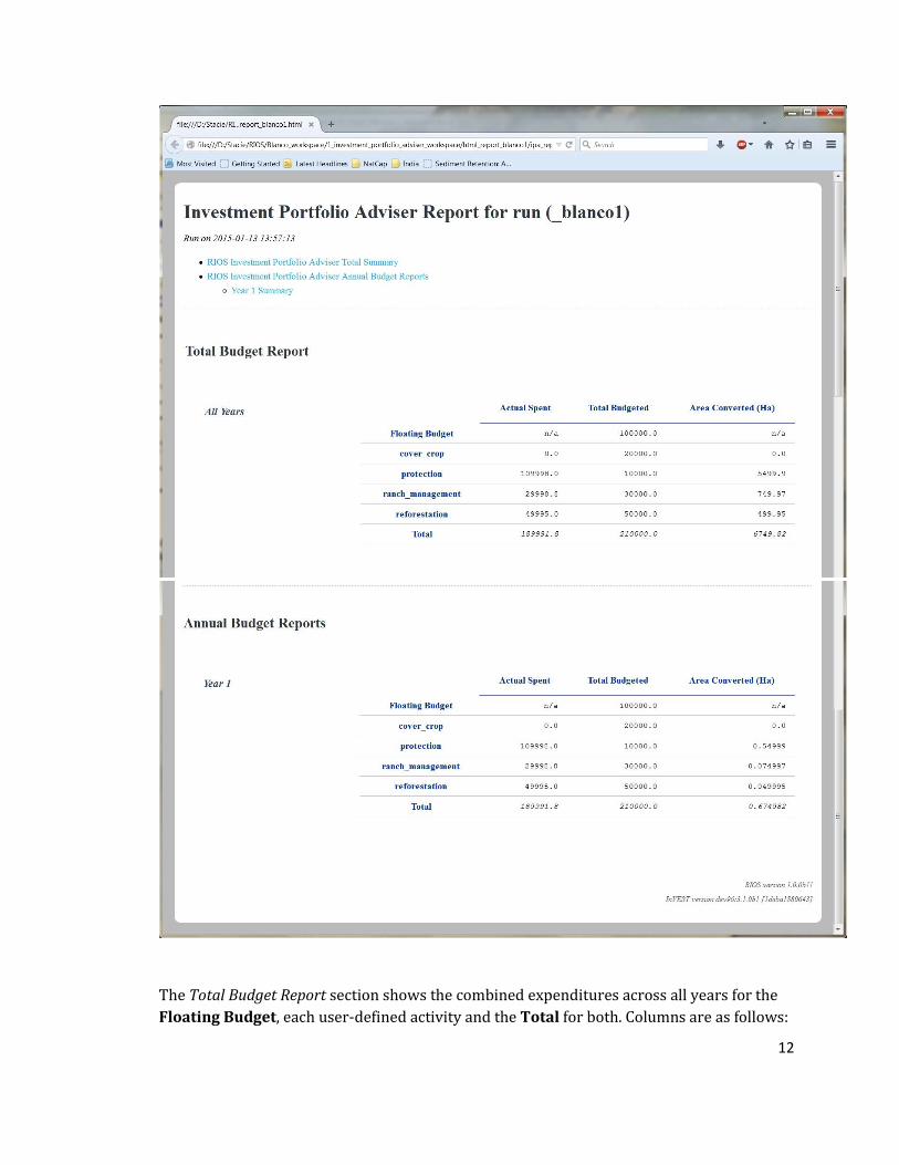
12

The Total Budget Report section shows the combined expenditures across all years for the

Floating Budget, each user-defined activity and the Total for both. Columns are as follows:

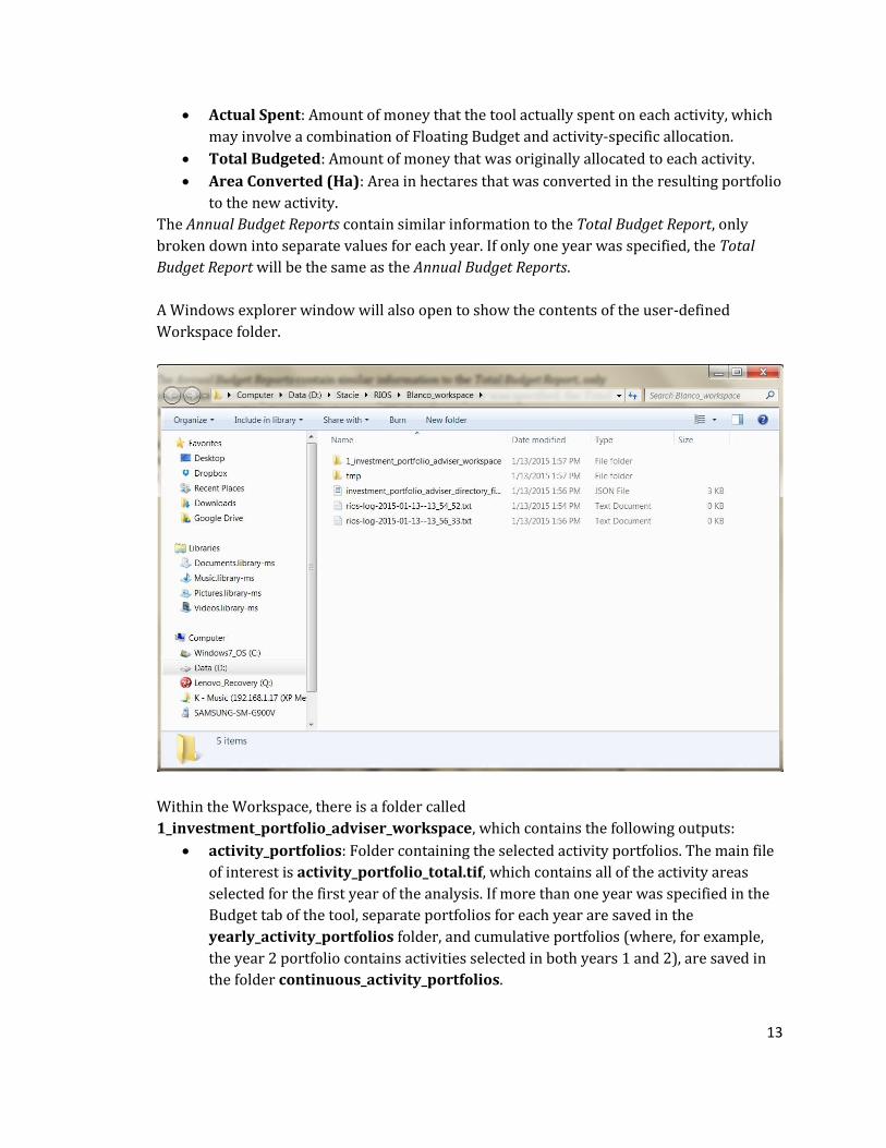
13

Actual Spent: Amount of money that the tool actually spent on each activity, which

may involve a combination of Floating Budget and activity-specific allocation.

Total Budgeted: Amount of money that was originally allocated to each activity.

Area Converted (Ha): Area in hectares that was converted in the resulting portfolio

to the new activity.

The Annual Budget Reports contain similar information to the Total Budget Report, only

broken down into separate values for each year. If only one year was specified, the Total

Budget Report will be the same as the Annual Budget Reports.

A Windows explorer window will also open to show the contents of the user-defined

Workspace folder.

Within the Workspace, there is a folder called

1_investment_portfolio_adviser_workspace, which contains the following outputs:

activity_portfolios: Folder containing the selected activity portfolios. The main file

of interest is activity_portfolio_total.tif, which contains all of the activity areas

selected for the first year of the analysis. If more than one year was specified in the

Budget tab of the tool, separate portfolios for each year are saved in the

yearly_activity_portfolios folder, and cumulative portfolios (where, for example,

the year 2 portfolio contains activities selected in both years 1 and 2), are saved in

the folder continuous_activity_portfolios.

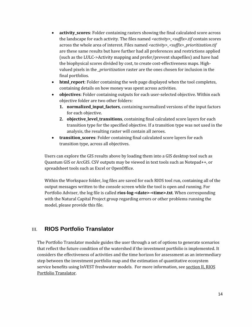
14

activity_scores: Folder containing rasters showing the final calculated score across

the landscape for each activity. The files named <activity>_<suffix>.tif contain scores

across the whole area of interest. Files named <activity>_<suffix>_prioritization.tif

are these same results but have further had all preferences and restrictions applied

(such as the LULC->Activity mapping and prefer/prevent shapefiles) and have had

the biophysical scores divided by cost, to create cost-effectiveness maps. High-

valued pixels in the _prioritization raster are the ones chosen for inclusion in the

final portfolios.

html_report: Folder containing the web page displayed when the tool completes,

containing details on how money was spent across activities.

objectives: Folder containing outputs for each user-selected objective. Within each

objective folder are two other folders:

1. normalized_input_factors, containing normalized versions of the input factors

for each objective.

2. objective_level_transitions, containing final calculated score layers for each

transition type for the specified objective. If a transition type was not used in the

analysis, the resulting raster will contain all zeroes.

transition_scores: Folder containing final calculated score layers for each

transition type, across all objectives.

Users can explore the GIS results above by loading them into a GIS desktop tool such as

Quantum GIS or ArcGIS. CSV outputs may be viewed in text tools such as Notepad++, or

spreadsheet tools such as Excel or OpenOffice.

Within the Workspace folder, log files are saved for each RIOS tool run, containing all of the

output messages written to the console screen while the tool is open and running. For

Portfolio Adviser, the log file is called rios-log-<date>-<time>.txt. When corresponding

with the Natural Capital Project group regarding errors or other problems running the

model, please provide this file.

III. RIOS Portfolio Translator

The Portfolio Translator module guides the user through a set of options to generate scenarios

that reflect the future condition of the watershed if the investment portfolio is implemented. It

considers the effectiveness of activities and the time horizon for assessment as an intermediary

step between the investment portfolio map and the estimation of quantitative ecosystem

service benefits using InVEST freshwater models. For more information, see section II, RIOS

Portfolio Translator.

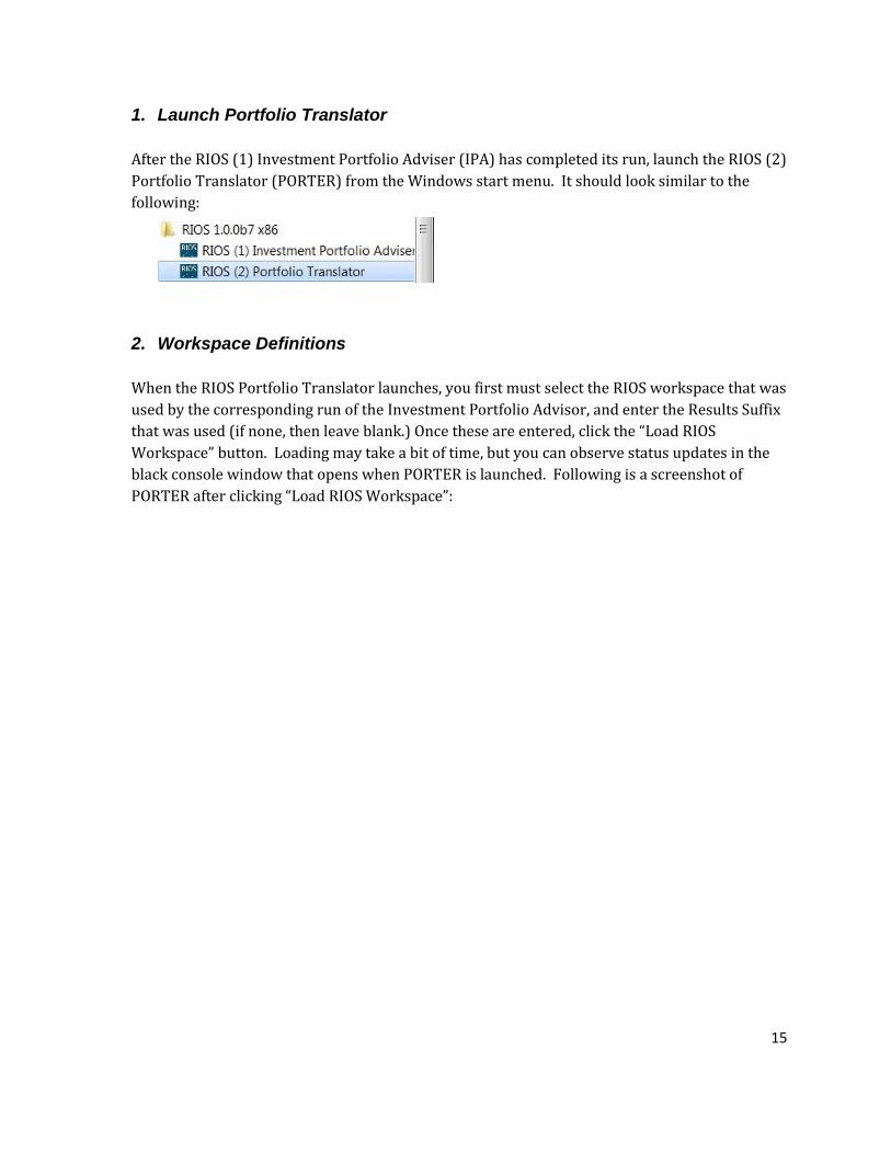
15

1. Launch Portfolio Translator

After the RIOS (1) Investment Portfolio Adviser (IPA) has completed its run, launch the RIOS (2)

Portfolio Translator (PORTER) from the Windows start menu. It should look similar to the

following:

2. Workspace Definitions

When the RIOS Portfolio Translator launches, you first must select the RIOS workspace that was

used by the corresponding run of the Investment Portfolio Advisor, and enter the Results Suffix

that was used (if none, then leave blank.) Once these are entered, click the “Load RIOS

Workspace” button. Loading may take a bit of time, but you can observe status updates in the

black console window that opens when PORTER is launched. Following is a screenshot of

PORTER after clicking “Load RIOS Workspace”:

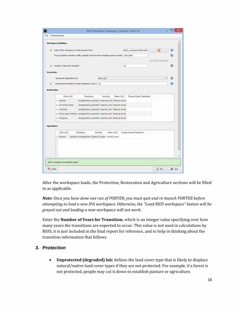
16

After the workspace loads, the Protection, Restoration and Agriculture sections will be filled

in as applicable.

Note: Once you have done one run of PORTER, you must quit and re-launch PORTER before

attempting to load a new IPA workspace. Otherwise, the “Load RIOS workspace” button will be

greyed out and loading a new workspace will not work.

Enter the Number of Years for Transition, which is an integer value specifying over how

many years the transitions are expected to occur. This value is not used in calculations by

RIOS, it is just included in the final report for reference, and to help in thinking about the

transition information that follows.

3. Protection

Unprotected (degraded) lulc defines the land cover type that is likely to displace

natural/native land cover types if they are not protected. For example, if a forest is

not protected, people may cut it down to establish pasture or agriculture.

17

Proportional transition is a value between 0 and 1 that indicates what proportion

of the natural land cover type is expected to transition over the Number of Years for

Transition specified above. For more information, see Protect Native Vegetation in

the RIOS Portfolio Translator section.

Note: Even if your analysis does not include a Protection activity, these values must be

filled in, but they will not affect your results.

4. Restoration

In the Restoration table, all of the Old LULC types in the base land cover map that were

chosen in the portfolio for a restoration Activity are listed, along with their associated

Transition type. The New LULC class that the Old LULC is predicted to transition to as a

result of the restoration is determined by the tool by looking around the Old LULC pixels

and selecting the native landcover type that is dominant nearby.

In the Proportional Transition column, enter a value between 0 and 1 indicating what

proportion of the Old LULC is likely to be transitioned to the New LULC in the Number of

Years specified. For more information, see Revegetation - assisted and Revegetation -

unassisted in the RIOS Portfolio Translator section.

5. Agriculture

The Agriculture table is similar to Restoration, where the Old LULC types in the base land

cover map that were chosen for an Agriculture activity are listed, along with the associated

Transition type. Proportional Transition must be filled in with values from 0 to 1 indicating

the effectiveness of the management activity.

Here, the New LULC column is user-selected to be a reference land cover class (which must

be an existing land cover class in the LULC raster) that represents the ‘ideal’ situation if the

parcel was to be perfectly managed. For more information, see Ditching, Fertilizer

management and Pasture management in the RIOS Portfolio Translator section.

6. Results

Once all entries have been filled in, click the Run button. When the tool is finished running, a

Windows explorer window will open to the Workspace location. Outputs from the Portfolio

Translator are found in the folder 2_portfolio_translator_lulc_scenarios. Inside this folder

are the following output files:

base_lulc.tif: Raster of the base (current) LULC map, which should be the same as

the LULC raster entered as an input into IPA

transitioned_lulc.tif: Raster combining the base LULC map and the areas selected

in the IPA-generated portfolio for restoration and agriculture transitions only. The

18

assumption here is that areas selected for protection are protected, and so retain

their original LULC types. Pixel values correspond to land use codes. See

transitioned_coefficients.csv below for more information on transition land use

codes.

unprotected_lulc.tif: Raster combining the base LULC map and the areas selected

in the IPA-generated portfolio for restoration and agriculture, as well as protection.

Areas that are selected for protection are assigned a new LULC class that indicates

the user-selected Unprotected (degraded) lulc. This result allows for modeling the

marginal benefit of protection, by calculating the change in ecosystem service that is

likely to occur as a result of not protecting these areas. Pixel values correspond to

land use codes. See unprotected_coefficients.csv below for more information on

transition land use codes.

base_coefficients.csv: Table containing biophysical coefficients for all base RIOS

land cover types in the base LULC raster. This corresponds to the LULC Biophysical

Coefficients table provided in the Portfolio Advisor.

transitioned_coefficients.csv: Table containing biophysical model coefficients for

both base and transitioned land cover types for restoration and agricultural

transitions (not protection.) Transitioned land cover types are described in the

LULC_desc field as <Old LULC>,<transition>,<activity>,<New LULC>. And they are

assigned new unique lucodes as <Old lucode><transition code>0<activity

code>0<New lucode>, where the Old and New lucodes are taken from the user-input

LULC raster.

Transition codes are assigned integer values during the IPA model run. Activity

codes correspond to the integer values assigned to activities in the IPA result

activity_portfolio_total.tif, starting with a value of 0.

An example LU_desc might read “bare soil, revegetation_unassisted, fencing,

temperate grassland” with a corresponding lucode of “2603033,” where “2” is the

lucode for “bare soil,” “6” is the transition code for “unassisted revegetation,” “03” is

the activity code for “fencing” and “33” is the lucode for “temperate grassland.”

Details on the calculations of transitioned coefficients are given in section II, RIOS

Portfolio Translator.

unprotected_coefficients.csv: Similar to transitioned_coefficients.csv, but contains

biophysical model coefficients for areas where unprotected native landcover has

transitioned to the user-selected Unprotected (degraded) lulc. Again, the base LULC

types and coefficients are included, as well as new transitioned LULC types and

lucodes. Transitioned land cover types are described in the LULC_desc field as <Old

LULC>,<transition>,<activity>,<New LULC> Landcover types that have the

19

transition of “keep_native_vegetation” are described as <Old

LULC>,<transition>,<New LULC>,”degraded.” An example LULC_desc might be

“temperate grassland, keep_native_vegetation, agriculture, degraded” with a

corresponding lucode of “33003,” where “33” is the lucode for “temperate

grassland” and “03” is the transition code for “keep native vegetation.” The

unprotected lucodes are defined differently than those for transitioned classes.

Within the Workspace folder, log files are saved for each RIOS tool run, containing all of the

output messages written to the console screen while the tool is open and running. For

Portfolio Translator, the log file is called rios_porter-log-<date>-<time>.txt. When

corresponding with the Natural Capital Project group regarding errors or other problems

running the model (e.g. through our User Forum), please provide this log file, as it is very

useful for helping with debugging.

7. Running InVEST

After reviewing the coefficients calculated by PORTER, and adjusting them as needed to reflect conditions in the area of interest, the LULC and table results from PORTER may now be used as inputs to the InVEST SDR and/or Water Yield models. Details on these models and how to run them can be found in the InVEST User Guide. Here is just brief guidance on how to use the PORTER outputs in these models.

As described in Estimating benefits of RIOS portfolios, either two or three runs of InVEST will be needed, depending on whether a protection activity is included in the analysis or not. If there is a protection activity, then three runs will be done, one for the ‘base’ (or current) landscape, one for the ‘transitioned’ scenario (consisting of restoration and agriculture activities only) and one for the ‘unprotected’ scenario (which includes areas selected for protection changed into a degraded land cover type.) If there is not a protection activity, then only the ‘base’ landscape and ‘transitioned’ scenario will be used.

For both the SDR and Water Yield models, the same instructions apply. The rasters output by PORTER called base_lulc.tif, transitioned_lulc.tif and (if a protection activity is included) unprotected_lulc.tif are used as Land Use inputs to these InVEST models. And the tables output by PORTER called base_coefficients.csv, transitioned_coefficients.csv and (optionally) unprotected_coefficients.csv are used as the corresponding Biophysical Table inputs for each of the runs.

Once the InVEST runs have been completed, use the information provided in Estimating benefits of RIOS portfolios to calculate the return on investment predicted by these models. For SDR, the difference in annual sediment export for each watershed or sub-watershed is likely to be of most interest; for water yield, the difference in annual water volume. Remember that unless the models are calibrated for your watershed, the results should be taken as relative changes only, which are useful for understanding the direction and

http://forums.naturalcapitalproject.org/

http://data.naturalcapitalandresilienceplatform.org/invest-releases/documentation/current_release/index.html

20

magnitude of change that activity implementation may have on these hydrologic services on an annual average basis.

Date post:	06-Feb-2018
Category:	Documents
Upload:	hoangmien
View:	223 times
Download:	2 times

Resource Investment Optimization System...

Documents