RESOURCES ALLOCATION IN INDOOR AND UNDERWATER VLC NETWORKS BY KHALED ABDUL-AZIZ AL-UTAIBI A Dissertation Presented to the DEANSHIP OF GRADUATE STUDIES In Partial Fulfillment of the Requirements for the Degree of DOCTOR OF PHILOSOPHY IN COMPUTER SCIENCE ENGINEERING KING FAHD UNIVERSITY OF PETROLEUM & MINERALS Dhahran, Saudi Arabia APRIL, 2019
Transcript
RESOURCES ALLOCATION IN INDOORAND UNDERWATER VLC NETWORKS
BY
KHALED ABDUL-AZIZ AL-UTAIBI
A Dissertation Presented to theDEANSHIP OF GRADUATE STUDIES
In Partial Fulfillment of the Requirementsfor the Degree of
DOCTOR OF PHILOSOPHY
IN
COMPUTER SCIENCE ENGINEERING
KING FAHD UNIVERSITYOF PETROLEUM & MINERALS
Dhahran, Saudi Arabia
APRIL, 2019
KING FAHD UNIVERSITY OF PETROLEUM & MINERALSDHAHRAN 31261, SAUDI ARABIA
DEANSHIP OF GRADUATE STUDIES
This dissertation, written by KHALED ABDUL-AZIZ AL-UTAIBI under thedirection of his dissertation adviser and approved by his dissertation committee, hasbeen presented to and accepted by the Dean of Graduate Studies, in partial fulfill-ment of the requirements for the degree of DOCTOR OF PHILOSOPHY INCOMPUTER SCIENCE ENGINEERING.
Figure 3.4: A solution representation of the assignment in Example 1.
58
3.2.3 Extended Solution Representation
As discussed in section 3.2.2, we have two representations of the RA solution: one
for the direct implementation and one for the Tetris-Game model. In the direct
implementation, there exists a total of N × T slots that can be allocated to M users.
If the slots are equally divided between users, then each user will have (N × T )/M
slots. Since the objective is to maximize the system data rate under the consideration
of partial fairness, some users may be allocated more slots than others as long as the
constraint in equation (2.8) is respected. Therefore, we decided to use K×T time-slots
instead of T time-slots as defined in the original problem, where K is an integer greater
than 1. This allows the initial solution generator to include extra assignments for each
user (K×N×T )/M . Then, it is up to the optimization algorithm to allocate the slots
to maximize the total data rate in the first T time-slots. Note that the assignments in
the remaining (K × T − T ) time-slots are not included in the calculation of the total
data rate, hence, they should be occupied by assignments with the least data rates.
The extended solution representation for direct implementation of the RA problem is
illustrated by an example in Fig. 3.5.
In the Tetris-Game model, the extension of the solution is done in a different
manner. Instead of using extra time-slots, we repeat each generated piece K times,
where K is an integer that can be selected based on experimental results. Then, the
optimization algorithm will try to pack the pieces into T rows of the Tetris board such
that the total data rate is maximized. The remaining pieces placed into rows grater
than T will not participate in the calculation of the total data rate.
59
Figure 3.5: An example of the proposed extended solution representation.
60
3.3 Generating Tetris Pieces
Our experiments show that metaheuristic algorithms converge faster when using the
Tetris model allocation as compared to the individual LED allocation. However,
generating all possible combinations of the pieces is intractable for practical problems.
This makes individual allocation more flexible in exploring the various assignment
combinations. In order to take advantage of both approaches, we use large pieces
with high weights and small pieces (single LED assignments) with low weights. The
large pieces speed up the search process, while small pieces enable the optimization
algorithm to explore more areas by merging individual assignments to form pieces
with new combinations. In Example 1, we can generate the assignment of the 2nd user
in T3 using either a single piece with (1, 1, 0, 0) or using two pieces with (1, 0, 0, 0)
and (0, 1, 0, 0) respectively.
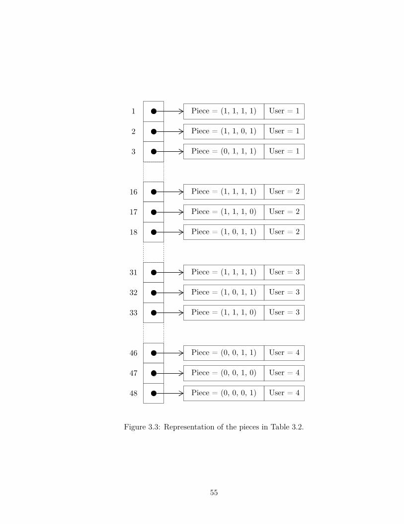
When generating the pieces for each user, we consider only LEDs with nonzero
channel-gain. In our Tetris model, we generate two sets of pieces for each user:
1. Single LED Allocation: consists of all combinations of pieces with a single
LED allocation. In Example 1, the first three users have four possible pieces
{(1, 0, 0, 0), (0, 1, 0, 0), (0, 0, 1, 0), (0, 0, 0, 1)}, while the last user has only two
possible pieces {(0, 0, 1, 0), (0, 0, 0, 1)}.
2. Multiple LEDs Allocation: consists of pieces with group of (2, 3, . . . , N) LEDs
selected based on their channel-gains ordered from highest to lowest. In Example
1, the first user has the following channel-gains (0.0966, 0.2943, 0.0884, 0.2527),
and his set of group allocations is given by {(0, 1, 0, 1), (1, 1, 0, 1), (1, 1, 1, 1)}.
61
Algorithm 1 shows how to generate the two sets of pieces for each user.
3.4 Placement of Pieces
In this section, we will discuss some terminologies for placing a piece in the Tetris
board:
• A piece p is said to be overlapping with an assignment A if there exists p′ ∈ A
such that (a′i = ai = 1) for some i (1 ≤ i ≤ N).
• Testing for the overlapping between a piece p and an assignment A is simply an
AND operation. We say that p overlaps with A if p ∧ A = 0.
• Adding a piece p to an assignment A is simply an OR operation (p ∨ A).
• Removing a piece p from an assignment A is simply an AND operation with the
complement of the piece (¬p ∨ A).
• The value of the piece that can fill the empty slots in an assignment A is given
by ¬A.
62
Algorithm 1: Procedure for generating the Tetris piecesInput : M , N , HOutput: Tetris
1 k ← 12 for i← 1 to M do3 /* Get channel-gains corresponding to the ith user */4 h← {H[i, 1], H[i, 2], . . . , H[i, N ]}5 /* Get the indices of nonzero channel-gains in h */6 hp ← {r|h[r] > 0, for 1 ≤ r ≤ N}7 /* Get the size of hp */8 Np ← |hp|9 /* Sort hp in descending order of the values of h */
10 (indices, values)← Sort(h)11 hp ← indices[1..Np]12 /* Generate single allocation set */13 for j ← 1 to Np do14 d← hp[j]15 Tetris[k].P ieces← (0, 0, . . . , 0)16 Tetris[k].P ieces[d]← 117 Tetris[k].User ← i18 k ← k + 1
19 end20 /* Generate multiple allocations set */21 for j ← 2 to Np do22 Tetris[k].P ieces← (0, 0, . . . , 0)23 Tetris[k].User ← i24 for m← 1 to j do25 d← hp[m]26 Tetris[k].P ieces[d]← 1
27 end28 k ← k + 1
29 end30 end31 return Tetris
63
CHAPTER 4
OPTIMIZATION HEURISTICS
BASED ON TETRIS GAME
MODEL
In order to demonstrate the effectiveness of our resource allocation model, we have
developed two metaheuristics for the indoor resource allocation problem. The first
algorithm is a direct application of the simulated annealing (DASA), and the second
is a Tetris-Game based simulated annealing (TGSA). The implementation details of
these algorithms are discussed in this chapter.
4.1 Initial Solution Generation
The simulated annealing (SA) starts from a random initial solution. In this section,
we discuss the implementation of the procedures that generate the initial solution for
both direct implementation and Tetris-Game model.
64
In the direct implementation of the RA problem, the initial solution is generated
randomly as shown in Algorithm 2. The procedure starts by generating an array A
from the set of elements {1, 2,×M} with each element repeated n times, where n is
the number of slots per user. If (K × N × T ) is not multiple of M , then tabbing is
used to fill the remaining elements of A. Next, the procedure rearranges the elements
of A in random order and assigns them to the slots in the solution Sinit.
Algorithm 2 shows the procedure for generating the initial solution for the Tetris-
Game model. The procedure starts by generating an array A from set of elements
{1, 2,×n} with each element repeated K times, where n is the number of pieces in
the Tetris array. Next, the procedure rearranges the elements of A in random order
and packs them into the Tetris board (i.e., the solution) in a first-fit manner. A piece
can be packed into a row if and only if it does not overlap with pieces already packed
in that row.
4.2 Simulated Annealing
Simulated annealing (SA) is a metaheuristic introduced by Kirpatrick et al. [70] in
1983, and independently by Černy [71] in 1985 to solve optimization problems with
large search spaces. The general structure of the SA and the Metropolis procedure are
shown in Algorithms 4 and 5 respectively [72]. The input to the algorithm consists
of 6 parameters (S0, T0, α, β, M0, MaxTime). The algorithm starts from an initial
solution S0 which can be generated randomly. In the beginning of the procedure, the
temperature is set to an initial value T0, and is decreased gradually using a cooling
65
rate α. The value of α is typically chosen in the range of 0.8 ≤ α ≤ 0.99. The initial
value of the time spent in the annealing process at a certain temperature is given
by the parameter M0. This time is gradually increased as the temperature decreases
using the parameter β. The total time for the annealing process is represented by the
parameter MaxTime.
The Metropolis procedure mimics the annealing operation at a certain temperature
T . This procedures receives 6 inputs which are the current solution and its cost (Scur,
Ccur), the best solution seen so far and its cost (Sbest, Cbest), the current temperature
T , and the parameter M which represents the amount of time need to be spent by the
annealing process at temperature T . The Metropolis procedure uses the procedure
Neighbor to generate a new solution Snew by doing a minor modification to the current
solution Scur. The cost of the new solution is evaluated by the function Cost. If the
cost of the new solution Snew is better than the cost of the current solution Scur, then
the current solution is updated by accepting the new solution. The same statement
applies to the best solution seen so far Sbest. The Metropolis procedure may accept a
solution with a higher cost with a probability p < e−∆C/T where ∆C is the difference
between the costs of the new and current solutions.
4.3 Implementation Details
In this section, we discuss the implementation details of the main functions of the
simulated annealing for both DASA and TGSA.
66
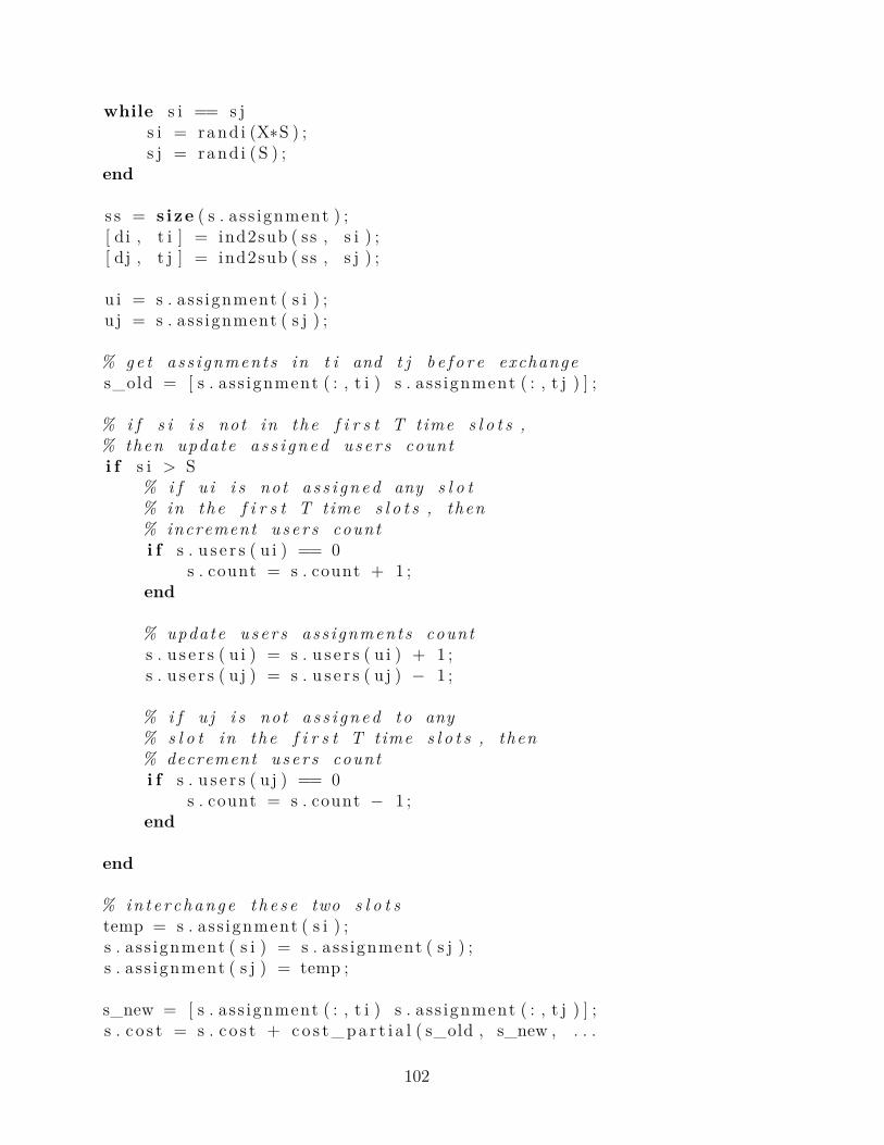
4.3.1 The Neighbor Function
In the SA algorithm, the neighbor function generates a new solution by making a minor
modification to the current solution. In the direct application of the SA algorithm to
the RA problem, we have implemented a simple neighbor function that exchanges the
assignment of two time-slots selected randomly as illustrated in Algorithm 6. Such
approach can not be used in the Tetris model as it may generate invalid solutions due
to overlapping pieces. Thus, before placing a piece p in a row r, the neighbor function
needs to make sure that p does not overlap with any piece already in r.
The neighbor function for the Tetris-Game model is described in Algorithm 7. This
function selects a random piece pout from a random row tout, and places it into another
random row tin. The function checks for overlapping between pout and existing pieces
in tin, and moves those pieces to tout. The function repeats the process of exchanging
overlapping pieces between tout and tin until there are no more overlaps. The row tout
is selected randomly from 1 to T , while tin is selected randomly from 1 to Ts, where
Ts is the total number of rows in the Tetris board (i.e., Tetris solution). In this way,
the TGSA algorithm can pack the pieces into T rows (time-slots) while maximizing
the total data rate.
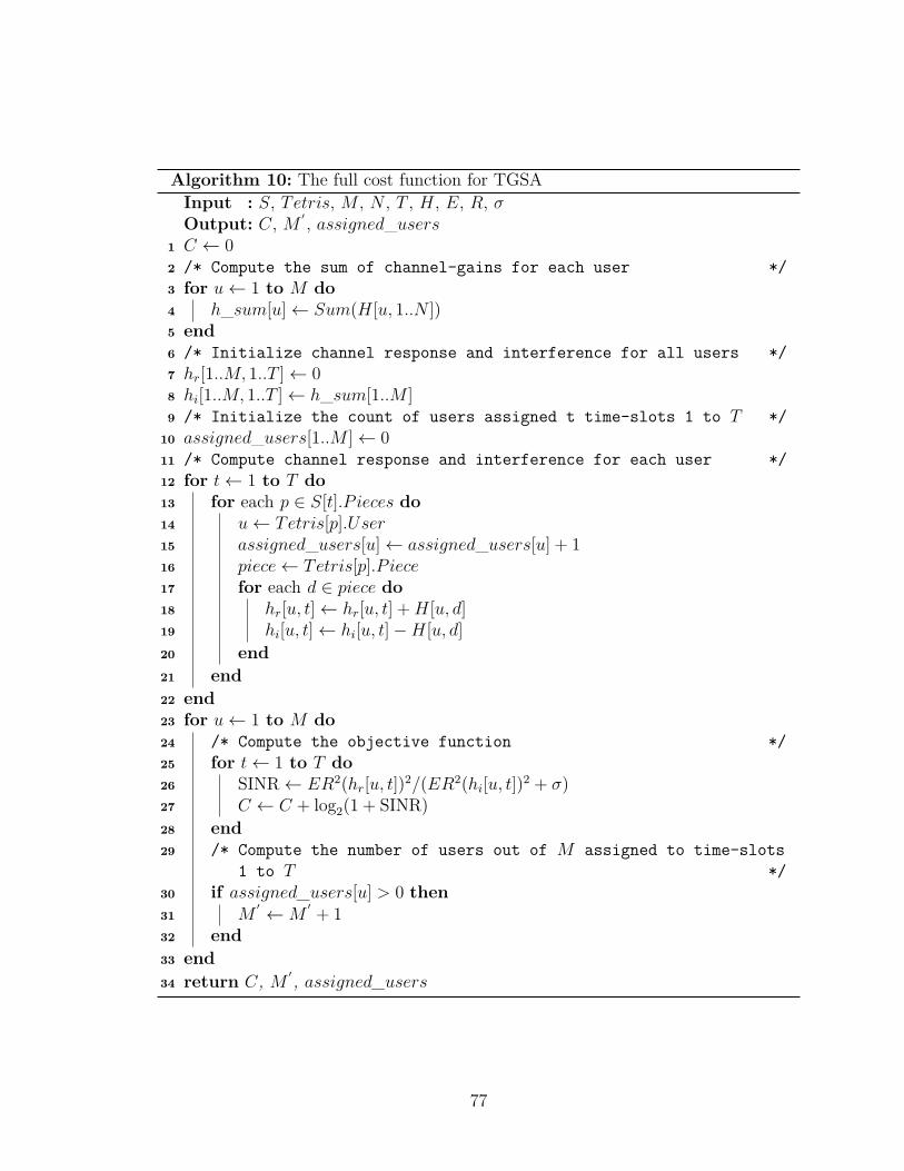
4.3.2 The Cost Function
The cost function in SA computes the objective function to be minimized or maxi-
mized. In the RA problem, our objective is to maximize the total data rate under the
consideration of partial fairness as given in equation (2.9. The objective function can
67
be computed is shown in Algorithm 9. We have implemented two cost functions for
both DASA and TGSA:
1. Full Cost Function: evaluates the objective function for the whole solution based
on equation (2.9) as shown in Algorithms. This function needs to be applied
only once on the initial solution.
2. Partial Cost Function: evaluates the objective function by recomputing the
SINR values for the modified slots of the neighbor solution as shown in Algo-
rithms.
In the DASA, the cost of the new solution (Cnew) is computed based on the on the
cost of the old solution (Cold) using the following formula:
Cnew =
Cold +∑
u∈{ux,uy}t∈{tx,ty}
log2(1 + SINRnew[u, t])
−∑
u∈{ux,uy}t∈{tx,ty}
log2(1 + SINRold[u, t])
tx ≤ T
Cold +∑
u∈{ux,uy}t=ty
log2(1 + SINRnew[u, t])
−∑
u∈{ux,uy}t=ty
log2(1 + SINRold[u, t])
tx > T
(4.1)
where ux and uy are the two exchanged user assignments in time-slots tx and
ty respectively, and SINRnew and SINRold are the SINR values computed based on
the assignments in the new and old solutions respectively. Note that assignments in
time-slots greater than T do not affect the calculation of the cost function.
68
In the TGSA, the cos tis computed using the following formula:
Cnew =
Cold +∑
u∈{uin∪uout}t∈{tin,tout}
log2(1 + SINRnew[u, t])
−∑
u∈{uin∪uout}t∈{tin,tout}
log2(1 + SINRold[u, t])
tout ≤ T
Cold +∑
u∈{uin∪uout}t=tin
log2(1 + SINRnew[u, t])
−∑
u∈{uin∪uout}t=tin
log2(1 + SINRold[u, t])
tout > T
(4.2)
where uin and uout are the set of users assigned to time-slots tin and tout respectively.
69
Algorithm 2: Generates the initial solution in the direct implementationInput : M , N , T , KOutput: Sinit
1 /* Determine the number of slots available for each user */2 n← (K ×N × T )/M3 /* Generate an array from the set of users with each user repeated
n times */4 A← {1, 2, . . . ,M}n5 /* Arrange the elements of A in random order */6 A← RandomPermutation(A)7 /* Assign the elements of A to the slots in the solution */8 k ← 19 for i← 1 to N do
10 for j ← 1 to K × T do11 Sinit[i, j]← A[k]12 k ← k + 1
13 end14 end15 return Sinit
70
Algorithm 3: Generates the initial solution in the Tetris-Game modelInput : M , N , T , K, TetrisOutput: Sinit
1 n← length(Tetris)2 /* Generate an array from the set of piece's indices in Tetris
with each index repeated K times */3 A← {1, 2, . . . , n}K4 /* Arrange the elements of A in random order */5 A← RandomPermutation(A)6 /* Initialize the solution */7 for i← 1 to K × n do8 S[i].Assignment← (0, 0, . . . , 0)9 S[i].P ieces← ϕ
10 end11 /* Pack the pieces idexed by A into the rows of Sinit in a
first-fit manner */12 k ← 113 for i← 1 to K × n do14 index← A[k]15 piece← Tetris[index].P iece16 k ← k + 117 for j ← 1 to K × n do18 /* Check for overlapping between the piece and the
assignment in the jth row */19 overlap← S[j].Assignment ∧ piece20 if ¬overlap then21 /* Merge the piece with the current assignment */22 S[j].Assignment← S[j].Assignment ∨ piece23 /* Add the index of the piece to the list of pieces in
the jth row */24 S[j].P ieces← S[j].P ieces ∪ {index}25 break26 end27 end28 /* Copy none empty rows in S into Sinit */29 k ← 130 for i← 1 to K × n do31 if S[i].Assignment ̸= (0, 0, . . . , 0) then32 Sinit[k] = S[i]33 k ← k + 1
Algorithm 5: The Metropolis procedureInput : Scur, Ccur, Sbest, Cbest, T , MOutput: Scur, Ccur, Sbest, Cbest
1 repeat2 Snew = Neighbor(Scur)3 Cnew = Cost(Ccur
4 ∆C = Cnew − Ccur
5 if ∆C < 0 then6 Scur = Snew
7 if Cnew < Cbest then8 Sbest = Snew
9 end10 else11 if RANDOM < e−∆C/T then12 Scur = Snew
13 end14 end15 M =M − 1
16 until M = 017 return Scur, Ccur, Sbest, Cbest
72
Algorithm 6: The neighbor function for DASA AlgorithmInput : S, N , T , KOutput: S
1 /* Select two different random slots from S */2 repeat3 tx ← RandomInteger(1..K × T )4 ty ← RandomInteger(1..T )5 dx ← RandomInteger(1..N)6 dy ← RandomInteger(1..N)
7 until tx ̸= ty or dx ̸= dy8 /* Exchange the two slots */9 Swap(S[dx, tx], S[dy, ty])
10 return S
73
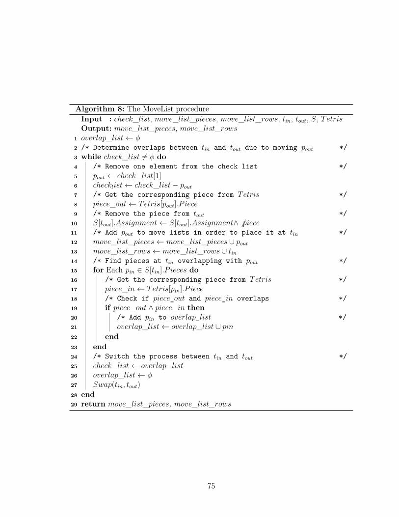
Algorithm 7: The neighbor function for TGSA AlgorithmInput : S, N , T , TetrisOutput: S
1 /* Get the total length of the solution S */2 Ns ← |S|3 /* Select two different random rows from S */4 repeat5 tout ← RandomInteger(1..Ts)6 tin ← RandomInteger(1..T )
7 until tout ̸= tin8 /* Select a random piece from tout */9 pout ← S[tout].P ieces[RandomInteger(1..Ns)]
10 /* Initialize lists */11 check_list← {pout}12 move_list_pieces← ϕ13 move_list_rows← ϕ14 MoveList(check_list,move_list_pieces,move_list_rows, tin, tout, S, Tetris)15 /* Place pieces in move list in their proper rows */16 for each p ∈ move_list_pieces and t ∈ move_list_rows do17 /* Get the piece details from the Tetris */18 piece← Tetris[p].P iece19 /* Place the piece */20 S[t].Assignment = piece ∨ S[t].Assignment21 S[t].P ieces = S[t].P ieces ∪ p22 end23 /* Check if tout row is empty, then delete it */24 if S[tout].P ieces = ϕ then25 Delete(S[tout])26 end27 return S
1 overlap_list← ϕ2 /* Determine overlaps between tin and tout due to moving pout */3 while check_list ̸= ϕ do4 /* Remove one element from the check list */5 pout ← check_list[1]6 checklist← check_list− pout7 /* Get the corresponding piece from Tetris */8 piece_out← Tetris[pout].P iece9 /* Remove the piece from tout */
10 S[tout].Assignment← S[tout].Assignment∧ ̸ piece11 /* Add pout to move lists in order to place it at tin */12 move_list_pieces← move_list_pieces ∪ pout13 move_list_rows← move_list_rows ∪ tin14 /* Find pieces at tin overlapping with pout */15 for Each pin ∈ S[tin].P ieces do16 /* Get the corresponding piece from Tetris */17 piece_in← Tetris[pin].P iece18 /* Check if piece_out and piece_in overlaps */19 if piece_out ∧ piece_in then20 /* Add pin to overlap_list */21 overlap_list← overlap_list ∪ pin22 end23 end24 /* Switch the process between tin and tout */25 check_list← overlap_list26 overlap_list← ϕ27 Swap(tin, tout)
28 end29 return move_list_pieces, move_list_rows
75
Algorithm 9: The full cost function for DASAInput : S, M , N , T , H, E, R, σOutput: C, M ′ , assigned_users
1 C ← 02 /* Compute the sum of channel-gains for each user */3 for u← 1 to M do4 h_sum[u]← Sum(H[u, 1..N ])5 end6 /* Initialize channel response and interference for all users */7 hr[1..M, 1..T ]← 08 hi[1..M, 1..T ]← h_sum[1..M ]9 /* Initialize the count of users assigned t time-slots 1 to T */
10 assigned_users[1..M ]← 011 /* Compute channel response and interference for each user */12 for d← 1 to N do13 for t← 1 to T do14 u← S[d, t]15 hr[u, t]← hr[u, t] +H[u, d]16 hi[u, t]← hi[u, t]−H[u, d]17 assigned_users[u]← assigned_users[u] + 1
18 end19 end20 for u← 1 to M do21 /* Compute the objective function */22 for t← 1 to T do23 SINR← ER2(hr[u, t])
2/(ER2(hi[u, t])2 + σ)
24 C ← C + log2(1 + SINR)
25 end26 /* Compute the number of users out of M assigned to time-slots
1 to T */27 if assigned_users[u] > 0 then28 M
′ ←M′+ 1
29 end30 end31 return C, M ′, assigned_users
76
Algorithm 10: The full cost function for TGSAInput : S, Tetris, M , N , T , H, E, R, σOutput: C, M ′ , assigned_users
1 C ← 02 /* Compute the sum of channel-gains for each user */3 for u← 1 to M do4 h_sum[u]← Sum(H[u, 1..N ])5 end6 /* Initialize channel response and interference for all users */7 hr[1..M, 1..T ]← 08 hi[1..M, 1..T ]← h_sum[1..M ]9 /* Initialize the count of users assigned t time-slots 1 to T */
10 assigned_users[1..M ]← 011 /* Compute channel response and interference for each user */12 for t← 1 to T do13 for each p ∈ S[t].P ieces do14 u← Tetris[p].User15 assigned_users[u]← assigned_users[u] + 116 piece← Tetris[p].P iece17 for each d ∈ piece do18 hr[u, t]← hr[u, t] +H[u, d]19 hi[u, t]← hi[u, t]−H[u, d]
20 end21 end22 end23 for u← 1 to M do24 /* Compute the objective function */25 for t← 1 to T do26 SINR← ER2(hr[u, t])
2/(ER2(hi[u, t])2 + σ)
27 C ← C + log2(1 + SINR)
28 end29 /* Compute the number of users out of M assigned to time-slots
1 to T */30 if assigned_users[u] > 0 then31 M
′ ←M′+ 1
32 end33 end34 return C, M ′, assigned_users
77
Algorithm 11: The partial cost function for DASAInput : Sold, Snew, Cold, M
′
old, assigned_users_old, N , T , tx, ty, ux, uy, H,E, R, σ
Output: Cnew, M ′new, assigned_users_new
1 Cnew ← Cold; M′new ←M
′
old
2 assigned_users_new ← assigned_users_old3 /* If ux and uy are identical, then the cost will be the same */4 if ux = uy then return Cnew, M ′
new, assigned_users_new5 /* Initialization */6 InitPartialCost(N , T , tx, ty, ux, uy, H)7 /* Update users counts */8 if tx > T then9 assigned_users_new[ux]← assigned_users_new[ux] + 1
13 end14 /* Compute channel response and interference for each user */15 for d← 1 to N do16 for j ← 1 to |tc| do17 uold ← Sold[d, tc[j]] ; unew ← Snew[d, tc[j]]18 for i← 1 to |uc| do19 if uold = uc[i] then20 holdr [i, j]← holdr [i, j] +H[i, d]; holdi [i, j]← holdi [i, j]−H[i, d]21 end22 if unew = uc[i] then23 hnewr [i, j]← hnewr [i, j] +H[i, d]; hnewi [i, j]← hnewi [i, j]−H[i, d]24 end25 end26 end27 end28 /* Update the objective function */29 for i← 1 to |uc| do30 for j ← 1 to |tc| do31 SINRold ← ER2(holdr [i, j])2/(ER2(holdi [i, j])2 + σ)32 SINRnew ← ER2(hnewr [i, j])2/(ER2(hnewi [i, j])2 + σ)33 Cnew ← Cnew + log2(1 + SINRnew)− log2(1 + SINRold)
34 end35 end36 return Cnew, M ′
new, assigned_users_new
78
Algorithm 12: The procedure InitPartialCost for DASAInput : N , T , tx, ty, ux, uy, HOutput: tc, uc, holdr , holdi , hnewr , hnewi
1 /* Initialize users lists */2 uc ← {uy, ux}3 /* Initialize time-slots lists */4 if tx ≤ T then5 /* Both slots will affect the cost, but not the user's counts
*/6 tc ← {ty, tx}7 else8 /* Only ty will affect the cost */9 tc ← {ty}
10 end11 /* Compute the sum of channel-gains for the 2 user */12 for i← 1 to 2 do13 h_sum[i]← Sum(H[uc[i], 1..N ])14 end15 /* Initialize channel response and interference for the 2 users */16 holdr [1..2, 1..2]← 017 holdi [1..2, 1..2]← h_sum[1..2]18 hnewr [1..2, 1..2]← 019 hnewi [1..2, 1..2]← h_sum[1..2]20 return tc, uc, holdr , holdi , hnewr , hnewi
79
Algorithm 13: The partial cost function for TGSAInput : Sold, Snew, Cold, Tetris, assigned_users_old, tout, tin, M , N , T , H,
E, R, σOutput: Cnew, M ′
new, assigned_users_new1 Cnew ← Cold ; M
′new ←M
′
old
2 assigned_users_new ← assigned_users_old3 InitPartialCost(M , N , T , tout, tin, H)4 /* Compute channel response and interference for each user */5 for i← 1 to |tc| do6 if tc[i] ≤ T then7 for each p ∈ Sold[tc[i]].P ieces do8 u← Tetris[p].User9 assigned_users[u]← assigned_users[u]− 1
10 if assigned_users[u] = 0 then M′new ←M
′new − 1;
11 piece← Tetris[p].P iece12 for each d ∈ piece do13 holdr [u, i]← holdr [u, i] +H[u, d] ; holdi [u, i]← holdi [u, i]−H[u, d]14 end15 end16 end17 if tc[i] ≤ T then18 for each p ∈ Snew[tc[i]].P ieces do19 u← Tetris[p].User20 assigned_users[u]← assigned_users[u] + 1
21 if assigned_users[u] = 1 then M′new ←M
′new + 1;
22 piece← Tetris[p].P iece23 for each d ∈ piece do24 hnewr [u, i]← hnewr [u, i] +H[u, d] ; hnewi [u, i]← hnewi [u, i]−H[u, d]25 end26 end27 end28 end29 for u← 1 to M do30 /* Update the objective function */31 if tc[i] ≤ T then32 for i← 1 to |tc| do33 SINRold ← ER2(holdr [u, i])2/(ER2(holdi [u, i])2 + σ)34 SINRnew ← ER2(hnewr [u, i])2/(ER2(hnewi [u, i])2 + σ)35 Cnew ← Cnew + log2(1 + SINRnew)− log2(1 + SINRold)
36 end37 end38 end39 return Cnew, M ′
new, assigned_users_new
80
Algorithm 14: The procedure InitPartialCost for TGSAInput : M , N , T , tout, tin, HOutput: tc, holdr , holdi , hnewr , hnewi
1 /* Initialize time-slots lists */2 if tout ≤ T then3 /* Both slots will affect the cost, but not the users counts */4 tc ← {tin, tout}5 else6 /* Only tin will affect the cost */7 tc ← {tin}8 end9 /* Compute the sum of channel-gains for all users */
10 for u← 1 to M do11 h_sum[u]← Sum(H[u, 1..N ])12 end13 /* Initialize channel response and interference for all users */14 holdr [1..M, 1..2]← 015 holdi [1..M, 1..2]← h_sum[1..M ]16 hnewr [1..M, 1..2]← 017 hnewi [1..M, 1..2]← h_sum[1..M ]18 return tc, holdr , holdi , hnewr , hnewi
81
CHAPTER 5
NUMERICAL RESULTS AND
DISCUSSION
As discussed in Chapter 4, we have developed two metaheuristics for the indoor re-
source allocation problem. The first algorithm is a direct application of the simulated
annealing (DASA) and the second is a simulated annealing algorithm based on the
Tetris-Game model (TGSA). In this chapter, we present the experimental results based
on these algorithms.
5.1 Indoor RA Optimization
In our simulation of the proposed model for indoor environment, we have considered
a room of size 12.0m× 12.0m× 3.0m with 16 LEDs on the ceiling spaced by 3.0m in
both directions as illustrated in Fig. 5.1. The number of users is varied from 16 to 64
and are randomly distributed in the room. Table 5.1 shows the system and channel
parameters used in our experiments [67]. The transmission power for each LED (P ) is
82
35 dBm. The optical to electrical conversion coefficient (R) is 0.28 A/W. The system
bandwidth (B) is 20 MHz. The noise density (N0) is 10−22 W/Hz. The detector area
of the receiver (A) and its FOV semiangle (Ψ1/2) are 1cm2 and 60o respectively. The
transmitter semiangle (Φ1/2) is also 60o.
We have implemented the proposed heuristic in MATLAB on 3.1 GHz Intel Core
i7 processor with 16GB RAM. The parameters of the SA algorithm are as follows:
α = 0.99, β = 1, T0 = 1.0, and M0 = 200. Due to the stochastic nature of the SA
algorithm, we did 100 trials on each experiment and average the result.
5.1.1 System Throughput Vs Number of Users
In this experiment, we have compared the system throughput with respect to the
number of users for both the direct application of the SA algorithm (DASA) and the
Tetris-Game model (TGSA). The results are presented in Fig. 5.2 which shows that
TGSA outperforms DASA as the number of users increases. Note that we have fixed
the number of time-slots per frame (T = 12), hence, the system throughput per user
decreases as the number of users increases.
5.1.2 System Throughput Vs Number of Iterations
In this experiment, we have run the DASA and TGSA algorithms for a fixed number
of iterations and compared their system throughput for 16 and 64 users. The best and
current costs of the DASA and TGSA algorithms for 16 users are shown in Fig. 5.3
and 5.4 respectively. Both figures show the expected behavior of a standard simulated
83
0 3 6 9 12
0
3
6
9
12
Figure 5.1: Distribution of LEDs in the room.
84
Table 5.1: System and channel parameters.Parameter Symbol ValueTransmission Power for each LED P 20 dBmO/E Conversion Coefficient R 0.28 A/WSystem Bandwidth B 5 MHzNoise Density N0 10−22 W/HzDetector Area (A) 1cm2
Receiver FOV Semiangle Ψ1/2 60o
Transmitter Semiangle Φ1/2 60o
85
16 24 32 48 64
Number of Users
0
20
40
60
80
100
120
140
160
180
Syst
em D
ata
Rat
e [M
bps]
DASA
TGSA
Figure 5.2: System throughput with respect to the number of users.
86
annealing algorithm with hill-climbing. Fig. 5.5 and 5.6 show comparisons between
the best cost of the TGSA and that of DASA for 16 and 64 users respectively. These
results show that the Tetris-Game model improves both the solution quality and the
convergence rate.
5.2 Underwater RA Optimization
We consider the same setup as for the indoor environment except that users can move
in the vertical direction. Assuming a pure water and LOS, the channel response can
be calculated as given in equation (2.6). Fig. 5.7 shows a comparison between the best
cost of TGSA and DASA for 16 users in underwater environment. The results show
a similar behaviour of both algorithms where TGSA converges faster than DASA.
5.3 Results Discussion and Future Work
Our experiments using standard simulated annealing algorithm show that the final
allocation of LEDs takes a form similar to the arrangement of the Tetris pieces. This
is illustrated in in Table 5.2 for an indoor environment with nine LEDs (N = 9), eight
users (M = 8) and eight time-slots per frame (T = 8). The channel-gains of the users
are shown in Table 5.3. This observation is consistent with the results obtained in
Section 5.1.2 which show clearly that TGSA converges faster than DASA as it operates
on groups of assignments rather than individual ones.
In future work, we are planning to investigate more meta-heuristics and optimize
the proposed algorithms to satisfy the the channel coherence time. In addition to that,
87
0 200 400 600 800 1000 1200 1400
Number of Iterations
50
100
150
200
250
300
350
400
450
500
550
Syst
em D
ata
Rat
es
DASA Current Cost
DASA Best Cost
Figure 5.3: Best and current costs of the DASA for 16 users.
88
0 200 400 600 800 1000 1200 1400
Number of Iterations
380
400
420
440
460
480
500
520
540
560
Syst
em D
ata
Rat
e
TGSA Best Cost
TGSA Current Cost
Figure 5.4: Best and current costs of the TGSA for 16 users.
89
0 200 400 600 800 1000 1200 1400
Number of Iterations
50
100
150
200
250
300
350
400
450
500
550
Syst
em D
ata
Rat
e
DASA Best Cost
TGSA Best Cost
Figure 5.5: Comparison of the best costs of TGSA and DASA for 16 users.
90
0 200 400 600 800 1000 1200 1400
Number of Iterations
0
100
200
300
400
500
Syst
em D
ata
Rat
e
TGSA Best Cost
DASA Best Cost
Figure 5.6: Comparison of the best costs of TGSA and DASA for 64 users.
91
0 200 400 600 800 1000 1200 1400
Number of Iterations
0
100
200
300
400
500
600
Syst
em D
ata
Rat
e
TGSA Best Cost
DASA Best Cost
Figure 5.7: Comparison of the best costs of TGSA and DASA for 16 users in under-water environment.
92
we will develop optimization heuristics for different types of water for the underwater
VLC problem (In our experiments, we considered only pure water types).
93
Table 5.2: Allocation result from a standard simulated annealing implementation for8 users, 9 LEDs and 8 time-slots per frame (M = 8, N = 9, T = 8).
%% Parametersglobal L W H LED PD M N T S A h h_sum E R sigma BW X;
% TDMA parametersM = 8 ; % number o f u s e r sN = 9 ; % number o f LEDsT = 8 ; % number o f time−s l o t sS = N ∗ T; % t o t a l number o f s l o t sA = f loor (S/M) ; % number o f s l o t s per userX = 16 ;L = 9 ; % room l e n g t hW = 9 ; % room widthH = 3 ; % room h e i g h t
E_dBm = 20 ; % symbol energy in dBmE = db2pow (E_dBm−30); % symbol energy in Watt 10 log_10 ( y )R = 0 . 2 8 ; % o p t i c a l to e l e c t r i c a l conver s i on
% c o e f f i c i e n tBW = 5e +6; % system bandwidth in Hz ( per LED)sigma = (1 e−22) ∗ BW; % no i s e power in Watt
95
squa r e s = sqrt (N) ; % number o f s quare s in each% row/column in the room
s t ep = L/ squa r e s ; % s e p a r a t i o n d i s t a n c e between% two LEDs
s t a r t = s t ep /2 ; % s t a r t i n g l o c a t i o n o f t he 1 s t LEDx = s t a r t : s t ep : L ; % x c o o r d i n a t e s o f t he LEDsy = x ; % y c o o r d i n a t e s o f t he LEDs
% compute the x−y−z c o o r i n a t e s o f t he LEDsLED = zeros (N, 3 ) ;LED( : , 3 ) = H;LED( : , 1 : 2 ) = combvec (x , y ) ’ ;
% genera t e x−y−z c o o r d i n a t e s o f t he u s e r s ( photo−d i ode s )PD = [ round ( rand (M, 1 ) ∗ L , 2 ) , . . .
% g e t channe l r e sponse sh = compute_channel_responses ( ) ;
load ( ’ v l c 8 . mat ’ , ’PD ’ , ’ h ’ ) ;
h_sum = sum(h , 2 ) ;
%% Simula ted Anneal ing Funct ions o l u t i o n = generate_random_solut ion ( ) ;% SA ParametersS0 = s o l u t i o n ; % i n i t i a l s o l u t i o nT0 = 1 ; % i n i t i a l t empera tureTf = 1 . 0 e−3; % f i n a l t empera turealpha = 0 . 9 9 5 ; % c o o l i n g r a t ebeta = 1 ; % cons tan tTp = 200 ; % time u n t i l t h e nex t
% parameter% update
Tc = T0 ; % curren t tempera tureCurS = S0 ; % curren t s o l u t i o nBestS = S0 ; % b e s t s o l u t i o n seenCurC = CurS . c o s t ∗ CurS . count / M; % curren t c o s tBestC = CurC ; % b e s t c o s t seenMaxIter = c o u n t _ i t e r a t i o n s (T0 , Tf , a lpha ) ;DASA_CC = zeros ( 1 , MaxIter ) ;DASA_BB = zeros ( 1 , MaxIter ) ;I t e r = 1 ;
96
while Tc > Tfcount = 0 ;while count < Tp
NewS = ne ighbor ( CurS ) ;NewC = NewS . c o s t ∗ NewS . count / M;DeltaC = NewC − CurC ;i f DeltaC > 0
CurS = NewS ;CurC = NewC;i f NewC > BestC
BestS = NewS ;BestC = NewC;
ende l s e i f rand <= exp ( DeltaC/Tc)
CurS = NewS ;CurC = NewC;
endcount = count + 1 ;
endDASA_CC_16( I t e r ) = CurC ;DASA_BB_16( I t e r ) = BestS . c o s t ;I t e r = I t e r + 1 ;
Tc = alpha ∗ Tc ;Tp = beta ∗ Tp ;
endfigure ( 1 ) ;p l o t _ s o l u t i o n ( BestS , 0 . 0 , BestC , 0 . 0 ) ;f igure ( 2 ) ;plot (DASA_CC) ;f igure ( 3 ) ;plot (DASA_BB) ;
%% Count Number o f I t e r a t i o n sfunction n = c o u n t _ i t e r a t i o n s (T0 , Tf , a lpha )n = 0 ;Tc = T0 ;while Tc > Tf
Tc = Tc ∗ alpha ;n = n + 1 ;
endend
%% Compute Cost ( F i t n e s s )
97
function f = c o s t _ p a r t i a l ( s_old , s_new , tx , ty , ux , uy )% computes the c o s t ( f i t n e s s ) o f a g i v en s o l u t i o nglobal N T h h_sum E R sigma ;
% i f the user i s t he same in% both s l o t s , then no change in the c o s ti f ux == uy
f = 0 ;return ;
end
% i n i t i a l i z e t he channe l r e sponse s /% i n t e r f e r e n c e s to be removed from the% o r i g i n a l s o l u t i o nRHSux = zeros ( 2 , 1 ) ;RHIux = [ h_sum( ux ) ; h_sum( ux ) ] ;RHSuy = zeros ( 2 , 1 ) ;RHIuy = [ h_sum( uy ) ; h_sum( uy ) ] ;
% i n i t i a l i z e t he channe l r e sponse s% / i n t e r f e r e n c e s to be added to the% mod i f i ed s o l u t i o nAHSux = zeros ( 2 , 1 ) ;AHIux = [ h_sum( ux ) ; h_sum( ux ) ] ;AHSuy = zeros ( 2 , 1 ) ;AHIuy = [ h_sum( uy ) ; h_sum( uy ) ] ;
% i n i t i a l i z e SINR f o r channe l r e sponse s to% be removed from the o r i g i n a l% s o l u t i o nRSINRux = zeros ( 2 , 1 ) ;RSINRuy = zeros ( 2 , 1 ) ;
% i n i t i a l i z e SINR f o r channe l r e sponse s% to be added to the mod i f i ed% s o l u t i o nASINRux = zeros ( 2 , 1 ) ;ASINRuy = zeros ( 2 , 1 ) ;
for d = 1 :N% g e t u s e r s ass i gnments in% t x and ty f o r the d^ th l e du_old = s_old (d , : ) ;u_new = s_new (d , : ) ;
98
% r e c a l c u l a t i o n f o r t ime s l o t t x w i l l% be done i f and on ly i f t x <= T and t x ~= tyi f tx <= T && tx ~= ty
i f u_old (1 ) == uxRHSux(1 ) = RHSux(1 ) + h( ux , d ) ;RHIux (1 ) = RHIux (1 ) − h( ux , d ) ;
e l s e i f u_old (1 ) == uyRHSuy(1 ) = RHSuy(1 ) + h( uy , d ) ;RHIuy (1 ) = RHIuy (1 ) − h( uy , d ) ;
end
i f u_new (1 ) == uxAHSux(1 ) = AHSux(1 ) + h( ux , d ) ;AHIux (1 ) = AHIux (1 ) − h( ux , d ) ;
e l s e i f u_new (1 ) == uyAHSuy(1 ) = AHSuy(1 ) + h( uy , d ) ;AHIuy (1 ) = AHIuy (1 ) − h( uy , d ) ;
endend
% r e c a l c u l a t i o n f o r t ime s l o t% ty w i l l be done in a l l c a s e si f u_old (2 ) == ux
%% Compute Cost ( F i t n e s s )function f = c o s t _ f u l l ( s o l u t i o n )% computes the c o s t ( f i t n e s s ) o f a g i v en s o l u t i o nglobal M N T h h_sum E R sigma ;
% i n i t i a l i z e SINRSINR = zeros (M,T) ;
ov e r a l l_a s s i gn ed_us e r s = zeros (M, 1 ) ;for t = 1 :T
% i n i t i a l i z e channe l r e sponse s and% i n t e r f e r e n c e in the t ^ th time−s l o ths = zeros (M, 1 ) ;h i = h_sum ;
% i n i t i a l i z e s e t o f a s s i gn ed us e r scur r ent_as s i gned_use r s = f a l s e (M, 1 ) ;
100
for d = 1 :N% g e t user ass ignmentu = s o l u t i o n . ass ignment (d , t ) ;
% s k i p unass i gned s l o t si f u == 0
h i ( : ) = h i ( : ) − h ( : , d ) ;cont inue ;
end
% compute channe l r e sponse s and% i n t e r f e r e n c e f o r the u^ th userhs (u ) = hs (u ) + h(u , d ) ;h i ( u ) = h i (u ) − h(u , d ) ;
% add user to the a s s i gned us e r s s e tcur r ent_as s i gned_use r s (u ) = t rue ;ov e r a l l_a s s i gn ed_us e r s (u ) = 1 ;
end% compute SINR f o r u s e r s a s s i gned% in the t ^ th t ime s l o t sfor u = 1 :M
i f cur r ent_as s i gned_use r s (u )SINR(u , t ) = E ∗ R^2 ∗ hs (u)^2 / . . .(E ∗ R^2 ∗ h i (u)^2 + sigma ) ;
endend
end% compute data r a t e per userDR = sum( log2 (1+SINR ) , 2 ) ;% compute the t o t a l data r a t ef = sum(DR, ’ a l l ’ ) ;end
%% Create Neighborfunction s = ne ighbor ( s o l u t i o n )% c r e a t e s a new s o l u t i o n by exchang ing two ass i gnments s e l e c t e d randomlyglobal S X;s = s o l u t i o n ;
% s e l e c t two d i f f e r e n t s l o t s randomlys i = 0 ;s j = 0 ;
101
while s i == s js i = rand i (X∗S ) ;s j = rand i (S ) ;
end
s s = s ize ( s . ass ignment ) ;[ di , t i ] = ind2sub ( ss , s i ) ;[ dj , t j ] = ind2sub ( ss , s j ) ;
u i = s . ass ignment ( s i ) ;u j = s . ass ignment ( s j ) ;
% g e t ass i gnments in t i and t j b e f o r e exchanges_old = [ s . ass ignment ( : , t i ) s . ass ignment ( : , t j ) ] ;
% i f s i i s not in the f i r s t T time s l o t s ,% then update a s s i gned us e r s counti f s i > S
% i f u i i s not a s s i gn ed any s l o t% in the f i r s t T time s l o t s , then% increment u s e r s counti f s . u s e r s ( u i ) == 0
s . count = s . count + 1 ;end
% update u s e r s ass i gnments counts . u s e r s ( u i ) = s . u s e r s ( u i ) + 1 ;s . u s e r s ( u j ) = s . u s e r s ( u j ) − 1 ;
% i f u j i s not a s s i gn ed to any% s l o t in the f i r s t T time s l o t s , then% decrement u s e r s counti f s . u s e r s ( u j ) == 0
s . count = s . count − 1 ;end
end
% in t e r change t h e s e two s l o t stemp = s . ass ignment ( s i ) ;s . ass ignment ( s i ) = s . ass ignment ( s j ) ;s . ass ignment ( s j ) = temp ;
s_new = [ s . ass ignment ( : , t i ) s . ass ignment ( : , t j ) ] ;s . c o s t = s . c o s t + c o s t _ p a r t i a l ( s_old , s_new , . . .
102
t i , t j , ui , u j ) ;end
%% Generate Random S o l u t i o n% g e n e r a t e s a random s o l u t i o n wi th e qua l t ime s l o t s f o r each userfunction s = generate_random_solut ion ( )global M N T A S X;
% i n t i a l i z e s o l u t i o n s t r u c t u r e% ass ignment : matr ix o f i n t% user ass ignment matr ix (LEDs x Time S l o t s )% c o s t : f l o a t% c o s t o f t he s o l u t i o n% use r s : v e c t o r o f i n t% number o f ass i gnments to each user in the f i r s t T s l o t s% count : i n t% number o f u s e r s out o f M as s i gned to the f i r s t T s l o t ss = s t r u c t ( ’ ass ignment ’ , zeros (N,X∗T) , . . .
’ c o s t ’ , 0 . 0 , . . .’ u s e r s ’ , zeros (M, 1 ) , . . .’ count ’ , 0 ) ;
% genera t e A random samples o f u s e r susers_samples = zeros (X∗A,M) ;for i = 1 :X∗A
users_samples ( i , : ) = randsample (M,M) ’ ;end
% a s s i g n t h e s e random samples to the NxT s l o t sfor i = 1 :X∗S
% g e t a random useruse r = users_samples ( i ) ;
% increment a s s i gned us e r s count in a l l s l o t s <= Ti f i <= S
i f s . u s e r s ( u s e r ) == 0s . count = s . count + 1 ;
ends . u s e r s ( u s e r ) = s . u s e r s ( u s e r ) + 1 ;
end
% a s s i g n users . ass ignment ( i ) = use r ;
103
ends . c o s t = c o s t _ f u l l ( s ) ;end
%% Plo t Room% p l o t t he room wi th LEDs and PDsfunction f = plot_room ( )global M PD LED L W;shgf = 0 ;% p l o t LEDs ’ l o c a t i o n ss c a t t e r (LED( : , 1 ) , LED( : , 2 ) , ’ b ’ ) ;
% p l o t PDs ’ l o c a t i o n shold on ;s c a t t e r (PD( : , 1 ) , PD( : , 2 ) , ’ r ’ ) ;grid minor ;axis ( [ 0 L 0 W] )
% d i s p l y users ’ l a b e l su s e r s = ( 1 :M) ’ ;l a b e l s = num2str ( use r s , ’%d ’ ) ;text (PD( : , 1 ) , PD( : , 2 ) , l a b e l s , . . .’ h o r i z o n t a l ’ , ’ l e f t ’ , ’ v e r t i c a l ’ , ’ bottom ’ ) ;
drawnow ;end
%% Plo t S o l u t i o n% p l o t s o l u t i o n as a heat−mapfunction f = p l o t _ s o l u t i o n ( s o l u t i o n , CurC , BestC , t )global T;shgf = 0 ;heatmap ( s o l u t i o n . ass ignment ( : , 1 :T ) ) ;s t r = sprintf ( ’ Current : ␣%f , ␣ Best : ␣%f , ␣ . . .Temp : ␣%f ’ ,CurC , BestC , t ) ;%t i t l e ( s t r ) ;drawnow ;end
A.2 MATLAB Code: Tetris Game Model Simu-lated Annealing
104
%% Parametersglobal L W H LED PD M N T S A h E R sigma t e t r i s BW h_sum ;
% TDMA parametersM = 16 ; % number o f u s e r sN = 16 ; % number o f LEDsT = 12 ; % number o f time−s l o t sS = N ∗ T; % t o t a l number o f s l o t s%A = f l o o r (S/M) ; % number o f s l o t s per userA = 18 ; % number o f p i e c e s o f each t e t r i s
% combinat ionL = 12 ; % room l e n g t hW = 12 ; % room widthH = 3 ; % room h e i g h tE_dBm = 20 ; % symbol energy in dBmE = db2pow (E_dBm−30); % symbol energy in Watt10log_10 ( y )R = 0 . 2 8 ; % o p t i c a l to e l e c t r i c a l
% conver s i on c o e f f i c i e n tBW = 5e +6; % system bandwidth in Hz ( per LED)sigma = (1 e−22) ∗ BW; % no i s e power in Wattsqua r e s = sqrt (N) ; % number o f s quare s in each
% row/column in the rooms t ep = L/ squa r e s ; % s e p a r a t i o n d i s t a n c e
% between two LEDss t a r t = s t ep /2 ; % s t a r t i n g l o c a t i o n o f t he 1 s t LEDx = s t a r t : s t ep : L ; % x c o o r d i n a t e s o f t he LEDsy = x ; % y c o o r d i n a t e s o f t he LEDs
% compute the x−y−z c o o r i n a t e s o f t he LEDsLED = zeros (N, 3 ) ;LED( : , 3 ) = H;LED( : , 1 : 2 ) = combvec (x , y ) ’ ;
% genera t e x−y−z c o o r d i n a t e s o f t he u s e r s ( photo−d i ode s )PD = [ round ( rand (M, 1 ) ∗ L , 2 ) , . . .
% g e t channe l r e sponse sh = compute_channel_responses ( ) ;
load ( ’ v l c 16 . mat ’ , ’PD ’ , ’ h ’ ) ;
h_sum = sum(h , 2 ) ;
105
% compute t e t r i s p i e c e st e t r i s = compute_tet r i s_p iece s ( ) ;
%% Simula ted Anneal ing% gene ra t e an i n i t a l random s o l u t i o ns o l u t i o n = generate_random_solut ion ( ) ;
% SA ParametersS0 = s o l u t i o n ; % i n i t i a l s o l u t i o nT0 = 1 ; % i n i t i a l t empera tureTf = 1 . 0 e−3; % f i n a l t empera turealpha = 0 . 9 9 5 ; % c o o l i n g r a t ebeta = 1 ; % cons tan tTp = 200 ; % time u n t i l t h e nex t parameter update
Tc = T0 ; % curren t tempera tureCurS = S0 ; % curren t s o l u t i o nBestS = S0 ; % b e s t s o l u t i o n seen so f a rCurC = CurS . c o s t ∗ CurS . users_count / M; % curren t c o s tBestC = CurC ; % b e s t c o s t seen so f a r
MaxIter = c o u n t _ i t e r a t i o n s (T0 , Tf , a lpha ) ;TGSA_CC = zeros ( 1 , MaxIter ) ;TGSA_BB = zeros ( 1 , MaxIter ) ;I t e r = 1 ;
while Tc > Tfcount = 0 ;while count < Tp
NewS = ne ighbor ( CurS ) ;NewC = NewS . c o s t ∗ NewS . users_count / M;DeltaC = (NewC − CurC ) ;i f DeltaC > 0
CurS = NewS ;CurC = NewC;i f NewC > BestC
BestS = NewS ;BestC = NewC;
ende l s e i f rand <= exp ( DeltaC/Tc)
CurS = NewS ;CurC = NewC;
endcount = count + 1 ;
end
106
%p l o t _ s o l u t i o n (CurS , CurS . cos t , BestS . cos t , Tc ) ;
TGSA_CC( I t e r ) = CurC ;TGSA_BB( I t e r ) = BestC ;I t e r = I t e r + 1 ;Tc = alpha ∗ Tc ;Tp = beta ∗ Tp ;
endfigure ( 1 ) ;p l o t _ s o l u t i o n ( BestS , 0 . 0 , BestC , 0 . 0 ) ;f igure ( 2 ) ;plot (TGSA_CC) ;f igure ( 3 ) ;plot (TGSA_BB) ;
%% Count Number o f I t e r a t i o n sfunction n = c o u n t _ i t e r a t i o n s (T0 , Tf , a lpha )n = 0 ;Tc = T0 ;while Tc > Tf
Tc = Tc ∗ alpha ;n = n + 1 ;
endend%% Neighborfunction s = ne ighbor ( s o l u t i o n )% c r e a t e s a new s o l u t i o n by removing% one p i e c e randomly from the g i v en% s o l u t i o n and a s s i g n i n g i t aga in in a random orderglobal t e t r i s N T;s = s o l u t i o n ;n = length ( s . s l o t s ) ;%% s t e p ( 1 ) : s e l e c t two random time% s l o t s t_out and t_in and random p i e c e%% s e l e c t two random time s l o t st_out = 0 ;t_in = 0 ;while t_out == t_in
t_out = rand i (n ) ;t_in = rand i (T) ;
end% s e l e c t random p i e c eindex = rand i ( s . s l o t s ( t_out ) . p i eces_count ) ;
107
% s t o r e o l d s l o t ss_old = [ s . s l o t s ( t_out ) s . s l o t s ( t_in ) ] ;
% s t o r e i n i t i a l t_out and t_in time−s l o tt_out_in i t = t_out ;t_ in_in i t = t_in ;
% i n i t i a l i z e o v e r l a p l i s to v e r l a p _ l i s t = zeros ( 1 ,N) ;
% i n i t i a l i z e check l i s tc h e c k _ l i s t = zeros ( 1 ,N) ;check_cnt = 1 ;c h e c k _ l i s t ( check_cnt ) = index ;
% i n i t i a l i z e move l i s tmove_l i s t_pieces = zeros ( 1 ,N) ;move_l i s t_s lo t s = zeros ( 1 ,N) ;move_cnt = 0 ;
%% s t e p ( 2 ) : move p_out to t_in and move% o v e r l a p p i n g p i e c e s between the s l o t s%while ( check_cnt > 0)
over lap_cnt = 0 ;i n s e r t e d _ o v e r l a p s = f a l s e (1 ,N) ;% f o r each p i e c e in the check l i s t% f i n d o v e r l a p i n g p i e c e sfor i = 1 : check_cnt
index_out = c h e c k _ l i s t ( i ) ;% g e t p i e c e ass ignment va l u ep_out = s . s l o t s ( t_out ) . p i e c e s ( index_out ) ;p iece_out = t e t r i s ( p_out ) . p i e c e ;
% remove the p i e c e from t_out s l o ts . s l o t s ( t_out ) . ass ignment = . . .and ( s . s l o t s ( t_out ) . ass ignment , ~piece_out ) ;s . s l o t s ( t_out ) . p i e c e s ( index_out ) = 0 ;s . s l o t s ( t_out ) . p i eces_count = . . .s . s l o t s ( t_out ) . p i eces_count − 1 ;% add the p i e c e to the move l i s t ,% so i t w i l l be p l a c ed a t t_inmove_cnt = move_cnt + 1 ;
108
move_l i s t_pieces ( move_cnt ) = p_out ;move_l i s t_s lo t s ( move_cnt ) = t_in ;
% check f o r o v e r l a p between p i e c e s% in the check l i s t and t ho s e in% t_infor index_in = 1 : s . s l o t s ( t_in ) . p i eces_count
% g e t p i e c e d e t a l i s
p_in = s . s l o t s ( t_in ) . p i e c e s ( index_in ) ;p i e ce_in = t e t r i s ( p_in ) . p i e c e ;
% e v a l u a t e o v e r l a p p i n g between the two p i e c e sove r l ap = any ( and ( piece_in , p iece_out ) ) ;
% check i f t h e two p i e c e s o v e r l a pi f ( ove r l ap )
% add the index o f o v e r l a p p i n g% p i e c e to o v e r l a p l i s ti f ~ i n s e r t e d _ o v e r l a p s ( index_in )
i n s e r t e d _ o v e r l a p s ( index_in ) = t rue ;over lap_cnt = over lap_cnt + 1 ;o v e r l a p _ l i s t ( over lap_cnt ) = index_in ;
endend
endend% remove p i c e s from t_outr ema in ing_piece s = . . .find ( s . s l o t s ( t_out ) . p i e c e s > 0 ) ;n = s . s l o t s ( t_out ) . p i eces_count ;s . s l o t s ( t_out ) . p i e c e s ( 1 : n ) = . . .s . s l o t s ( t_out ) . p i e c e s ( r ema in ing_piece s ) ;s . s l o t s ( t_out ) . p i e c e s (n+1:end ) = 0 ;% update check l i s tc h e c k _ l i s t = o v e r l a p _ l i s t ;check_cnt = over lap_cnt ;
% swap the two time s l o t st = t_in ;t_in = t_out ;t_out = t ;
end
t_out = t_out_in i t ;
109
t_in = t_in_in i t ;
%% s t e p ( 3 ) : p l a c e p i e c e s in move l i s t% in t h e i r proper t ime s l o t s%% f o r each e lement in the move l i s tfor i = 1 : move_cnt
% g e t e lement d e t a l i sp = move_l i s t_pieces ( i ) ;t = move_l i s t_s lo t s ( i ) ;
% g e t the p i e c e d e t a i l s from the t e t r i s l i s tp i e c e = t e t r i s (p ) . p i e c e ;u = t e t r i s ( p ) . u s e r ;
% update u s e r s count i f t_out > Ti f t_out > T
i f t <= Ti f s . u s e r s (u ) == 0
s . users_count = s . users_count + 1 ;ends . u s e r s (u ) = s . u s e r s (u ) + 1 ;
elses . u s e r s (u ) = s . u s e r s (u ) − 1 ;i f s . u s e r s (u ) == 0
s . users_count = s . users_count − 1 ;end
endend
% p l a c e the p i e c es . s l o t s ( t ) . ass ignment = or ( p i ece , s . s l o t s ( t ) . ass ignment ) ;n = s . s l o t s ( t ) . p i eces_count ;s . s l o t s ( t ) . p i e c e s (n+1) = p ;s . s l o t s ( t ) . p i eces_count = n + 1 ;
end
% s t o r e new s l o t ss_new = [ s . s l o t s ( t_out ) s . s l o t s ( t_in ) ] ;
%% s t e p ( 4 ) : remove i n i t i a l t_out time−s l o t i f i t i s empty%i f s . s l o t s ( t_out ) . p i eces_count == 0
110
% remove empty t ime s l o t ss . s l o t s ( t_out ) = [ ] ;
end
f = c o s t _ p a r t i a l ( s_old , s_new , [ t_out t_in ] ) ;%di s p ( f ) ;%d i s p ( s . c o s t ) ;s . c o s t = s . c o s t + f ;%di s p ( s . c o s t ) ;end
%% Generate Random S o l u t i o nfunction s o l u t i o n = generate_random_solut ion ( )% genera t e a random s o l u t i o nglobal N M T t e t r i s A;
% g e t the t o t a l number o f p i e c e s in the t e t r i sn = length ( t e t r i s ) ;
% s o l u t i o n ( ass ignment ) s t r u c t u r e% ass ignment : l o g i c a l v e c t o r s i z e N% merges a l l p i e c e s i n t o to a time−s l o t% p i e c e s : i n t v e c t o r o f s i z e N% con ta in s the indec e s o f ass ignment p i e c e s% pieces_count : i n t% counts number o f used p i e c e s% use r s : i n t v e c t o r o f s i z e M% number o f ass i gnments to each user in the f i r s t T s l o t s% users_count : i n t% number o f u s e r s out o f M as s i gned to the f i r s t T s l o t s% c o s t : f l o a t% c o s t ( f i t n e s s ) o f t he s o l u t i o n
s o l u t i o n = s t r u c t ( ’ s l o t s ’ , repmat ( s t r u c t ( . . .’ ass ignment ’ , f a l s e ( 1 ,N) , . . .’ p i e c e s ’ , zeros ( 1 ,N) , . . .’ p i eces_count ’ , 0 ) , n∗A, 1 ) , . . .’ u s e r s ’ , zeros ( 1 ,M) , . . .’ users_count ’ , 0 , . . .’ c o s t ’ , 0 . 0 ) ;
% genera t e a random sample from the t e t r i st e t r i s_samp l e = randsample (n∗A, n∗A) ;t e t r i s_samp l e = mod( te t r i s_sample , n ) + 1 ;n = n ∗ A;
111
for i = 1 : length ( t e t r i s_samp l e )% g e t the index o f t he i ^ th sample ( p i e c e )index = te t r i s_samp l e ( i ) ;
% g e t the p i e c e from the t e t r i sp i e c e = t e t r i s ( index ) . p i e c e ;
for t = 1 : n% g e t the ass ignment in the t ^ th% s o l u t i o n ( t ^ th time−s l o t )ass ignment = s o l u t i o n . s l o t s ( t ) . ass ignment ;
% check o v e r l a p p i n g between the i ^ th% p i e c e and t ^ th time−s l o tove r l ap = and ( p i ece , ass ignment ) ;
% i f no over l ap , then do the f o l l o w i n gi f ~ ove r l ap
% merge the p i e c e wi th the% cur r en t ass ignments o l u t i o n . s l o t s ( t ) . ass ignment = . . .or ( p i ece , ass ignment ) ;
% add the index o f t he a s s i gned p i e c em = s o l u t i o n . s l o t s ( t ) . p i eces_count ;s o l u t i o n . s l o t s ( t ) . p i e c e s (m+1) = index ;s o l u t i o n . s l o t s ( t ) . p i eces_count = m + 1 ;break ;
endend
end
empty_slots = zeros (n , 1 ) ;k = 0 ;
for t = 1 : ni f s o l u t i o n . s l o t s ( t ) . p i eces_count == 0
% i f time−s l o t i s empty , then add i t to the empty−s l o t s l i s tk = k + 1 ;empty_slots ( k ) = t ;
endend
% d e l e t e empty time−s l o t s from the s o l u t i o n
112
s o l u t i o n . s l o t s ( empty_slots ( 1 : k ) ) = [ ] ;
for t = 1 :T% update u s e r s count f o r cur r en t time−s l o tfor i = 1 : s o l u t i o n . s l o t s ( t ) . p i eces_count
p = s o l u t i o n . s l o t s ( t ) . p i e c e s ( i ) ;u = t e t r i s ( p ) . u s e r ;i f s o l u t i o n . u s e r s (u ) == 0
s o l u t i o n . users_count = s o l u t i o n . users_count + 1 ;ends o l u t i o n . u s e r s (u ) = s o l u t i o n . u s e r s (u ) + 1 ;
endend
s o l u t i o n . c o s t = c o s t ( s o l u t i o n ) ;end
%% Compute S o l u t i o n Cost ( F i t n e s s )function f = c o s t _ p a r t i a l ( s_old , s_new , t )% computes the c o s t ( f i t n e s s ) o f a g i v en s o l u t i o nglobal t e t r i s M T h E R sigma h_sum ;
% i n i t i a l i z e channe l r e sponse s to be removed from t_out and t_inRHs = zeros (M, 2 ) ;RHi = ones (M, 2 ) . ∗ h_sum ;
% i n i t i a l i z e channe l r e sponse s to be added to t_out and t_inAHs = zeros (M, 2 ) ;AHi = ones (M, 2 ) . ∗ h_sum ;
% i n i t i a l i z e SINR to be removed from t_out and t_inRSINR = zeros (M, 2 ) ;
% i n i t i a l i z e SINR to be added to t_out and t_inASINR = zeros (M, 2 ) ;
% i n i t i a l i z e added /removed us e r susers_removed = f a l s e (M, 2 ) ;users_added = f a l s e (M, 2 ) ;
% compute channe l r e sponse s o f to% be removed and addedfor i = 1 : 2
% compute channe l r e sponse s to be% removed from t_out and t_in
113
for j = 1 : s_old ( i ) . p i eces_count% g e t p i e c e d e t a i l sp = s_old ( i ) . p i e c e s ( j ) ;p i e c e = t e t r i s (p ) . p i e c e ;u = t e t r i s ( p ) . u s e r ;
% update removed us e r susers_removed (u , i ) = t rue ;
% determine a c t i v e−l e d s in the% p i e c e ass ignmenta c t i v e _ l e d s = find ( p i e c e > 0 ) ;
% determine the sum o f channe l% re sponse s o f a c t i v e _ l e d shh = sum(h (u , a c t i v e _ l e d s ) ) ;
% remove channe l r e sponse s i f and on ly i f t <= Ti f t ( i ) <= T
RHs(u , i ) = RHs(u , i ) + hh ;RHi (u , i ) = RHi(u , i ) − hh ;
endend
% compute channe l r e sponse s to% be added to t_out and t_infor j = 1 : s_new ( i ) . p i eces_count
% g e t p i e c e d e t a i l sp = s_new ( i ) . p i e c e s ( j ) ;p i e c e = t e t r i s (p ) . p i e c e ;u = t e t r i s ( p ) . u s e r ;
% update added us e r susers_added (u , i ) = t rue ;
% determine a c t i v e−l e d s in the p i e c e ass ignmenta c t i v e _ l e d s = find ( p i e c e > 0 ) ;
% determine the sum o f channe l% re sponse s o f a c t i v e _ l e d shh = sum(h (u , a c t i v e _ l e d s ) ) ;
% add channe l r e sponse s i f and on ly i f t <= Ti f t ( i ) <= T
AHs(u , i ) = AHs(u , i ) + hh ;
114
AHi(u , i ) = AHi(u , i ) − hh ;end
endend
% compute incrementa l c o s tf = 0 ;for u = 1 :M
for i = 1 : 2% compute SINR to be removedi f users_removed (u , i )
RSINR(u , i ) = E ∗ R^2 ∗ RHs(u , i )^2 / . . .(E ∗ R^2 ∗ RHi(u , i )^2 + sigma ) ;
end% compute SINR to be addedi f users_added (u , i )
ASINR(u , i ) = E ∗ R^2 ∗ AHs(u , i )^2 / . . .(E ∗ R^2 ∗ AHi(u , i )^2 + sigma ) ;
endf = f + log2 (1 + ASINR(u , i ) ) − log2 (1 + RSINR(u , i ) ) ;
endend
%unass igned_users = M − t o t a l_a s s i gned_use r s ;%f = f − f /M ∗ unass igned_users ;
end
%% Compute S o l u t i o n Cost ( F i t n e s s )function f = c o s t _ f u l l ( s o l u t i o n )% computes the c o s t ( f i t n e s s ) o f a g i v en s o l u t i o nglobal t e t r i s M T h E R sigma h_sum ;
% i n i t i a l i z e SINRSINR = zeros (M,T) ;
s = s o l u t i o n ;
% i n i t i a l i z e channe l r e sponse s and% i n t e r f e r e n c e s f o r a l l u s e r shs = zeros (M,T) ;h i = ones (M,T) . ∗ h_sum ;
for t = 1 :T
115
% i n i t i a l i z e a c t i v e u s e r s in cur r en t t ime s l o tac t i v e_us e r s = f a l s e (1 ,M) ;
% compute channe l r e sponse s and i n t e r f e r e n c e% in the t ^ th time−s l o tfor i = 1 : s . s l o t s ( t ) . p i eces_count
% f o r each p i e c e p in the assignment ,% g e t t he user and ass ignment% va l u ep = s . s l o t s ( t ) . p i e c e s ( i ) ;u = t e t r i s ( p ) . u s e r ;p i e c e = t e t r i s (p ) . p i e c e ;
% update a c t i v e u s e r sac t i v e_us e r s (u ) = t rue ;
% determine a c t i v e−l e d s in% the p i e c e ass ignmenta c t i v e _ l e d s = find ( p i e c e > 0 ) ;
% determine the sum o f channe l% re sponse s o f a c t i v e _ l e d shh = sum(h (u , a c t i v e _ l e d s ) ) ;
% update channe l r e sponse s% and i n t e r f e r e n c e v a l u e shs (u , t ) = hs (u , t ) + hh ;h i (u , t ) = h i (u , t ) − hh ;
end
% compute SINR f o r u s e r s a s s i gned% in the t ^ th t ime s l o t sfor u = 1 :M
i f ac t i v e_us e r s (u )SINR(u , t ) = E ∗ R^2 ∗ hs (u , t )^2 / . . .(E ∗ R^2 ∗ h i (u , t )^2 + sigma ) ;
endend
end
% compute data r a t e per userDR = sum( log2 (1+SINR ) , 2 ) ;% compute the t o t a l data r a t ef = sum(DR, ’ a l l ’ ) ;%unass igned_users = M − t o t a l_a s s i gned_use r s ;
116
%f = f − f /M ∗ unass igned_users ;
end
%% Compute S o l u t i o n Cost ( F i t n e s s )function f = c o s t ( s o l u t i o n )% computes the c o s t ( f i t n e s s ) o f a g i v en s o l u t i o nglobal t e t r i s M T h E R sigma ;
% i n i t i a l i z e SINRSINR = zeros (M,T) ;
s = s o l u t i o n ;
a s s i gned_use r s = f a l s e (M, 1 ) ;t o t a l_as s i gned_use r s = 0 ;
for t = 1 :T% i n i t i a l i z e channe l r e sponse s and% i n t e r f e r e n c e in the t ^ th time−s l o ths = zeros (M, 1 ) ;h i = zeros (M, 1 ) ;
% g e t ass ignment in the t ^ th t ime s l o tass ignment = s . s l o t s ( t ) . ass ignment ;n = s . s l o t s ( t ) . p i eces_count ;p i e c e s = s . s l o t s ( t ) . p i e c e s ( 1 : n ) ;
% determine a c t i v e−l e d e s in the ass ignmenta c t i v e _ l e d s = find ( ass ignment > 0 ) ;
% determine us e r s in the ass ignmentu s e r s = f a l s e (1 ,M) ;
% i n i t i a l i z e channe l i n t e r f e r e n c e f o r%the u s e r s a s s i gned to a c t i v e−l e d s%h i ( u s e r s ) = sum( h ( users , a c t i v e _ l e d s ) , 2 ) ;
% compute channe l r e sponse s and%i n t e r f e r e n c e in the t ^ th time−s l o tfor p = p i e c e s
% f o r each p i e c e p in the assignment ,% g e t t he user and ass ignment% va l u e
117
use r = t e t r i s ( p ) . u s e r ;p i e c e = t e t r i s (p ) . p i e c e ;
i f ~ as s i gned_use r s ( u s e r )a s s i gned_use r s ( u s e r ) = t rue ;t o t a l_as s i gned_use r s = to ta l_as s i gned_use r s + 1 ;
end
u s e r s ( u s e r ) = t rue ;
% determine a c t i v e−l e d s in the p i e c e ass ignmentuse r_ac t iv e_ l eds = find ( p i e c e > 0 ) ;
% determine the sum o f channe l r e sponse s o f a c t i v e _ l e d sh_sum = sum(h ( user , u s e r_ac t iv e_ l eds ) ) ;
% update channe l r e sponse s and% i n t e r f e r e n c e v a l u e shs ( u s e r ) = hs ( u s e r ) + h_sum ;h i ( u s e r ) = h i ( u s e r ) − h_sum ;
endac t i v e_us e r s = find ( u s e r s ) ;h i ( a c t i v e_us e r s ) = h i ( a c t i v e_us e r s ) + . . .sum(h ( ac t ive_use r s , a c t i v e _ l e d s ) , 2 ) ;
% compute SINR f o r u s e r s a s s i gned% in the t ^ th t ime s l o t sfor use r = ac t i v e_us e r s
SINR( user , t ) = E ∗ R^2 ∗ hs ( u s e r )^2 / . . .(E ∗ R^2 ∗ h i ( u s e r )^2 + sigma ) ;
endend
% compute data r a t e per userDR = sum( log2 (1+SINR ) , 2 ) ;% compute the t o t a l data r a t ef = sum(DR, ’ a l l ’ ) ;end
%% Plo t Roomfunction f = plot_room ( )% p l o t s LEDs and use r s l o c a t i o n sglobal M PD LED L W;shgf = 0 ;
118
% show LEDs and use r s l o c a t i o n s on a% s c a t t e r p l o ts c a t t e r (LED( : , 1 ) , LED( : , 2 ) ) ;grid minor ;axis ( [ 0 L 0 W] )hold on ;s c a t t e r (PD( : , 1 ) , PD( : , 2 ) ) ;% l a b e l u s e r s on the p l o tu s e r s = ( 1 :M) ’ ;l a b e l s = num2str ( use r s , ’%d ’ ) ;text (PD( : , 1 ) , PD( : , 2 ) , l a b e l s , ’ h o r i z o n t a l ’ , . . .’ l e f t ’ , ’ v e r t i c a l ’ , ’ bottom ’ ) ;drawnow ;end
%% Plo t Assignmentfunction f = p l o t _ s o l u t i o n ( s o l u t i o n , . . .
CurFitness , Bes tF i tne s s , Tc )% show the users ’ ass ignment on heat−map p l o t% map the s o l u t i o n to an NxT matr ixmap = map_solution ( s o l u t i o n ) ;shgf = 0 ;% show the ass ignment on a heat−mapheatmap (map ) ;% d i s p l y t he cur r en t+b e s t f i t n e s s e s% and cur r en t tempera tures = sprintf ( ’ Current : ␣%f , ␣ Best : ␣%f , ␣Temp : ␣ . . .␣␣␣␣%f ’ , CurFitness , Bes tF i tne s s , Tc ) ;t i t l e ( s ) ;drawnow ;end%% Map S o l u t i o nfunction map = map_solution ( s o l u t i o n )% maps a s o l u t i o n o f a s t r i p s−game% problem to an NxT matr ixglobal N t e t r i s T;%T = l e n g t h ( s o l u t i o n ) ;map = zeros (N,T) ;for t = 1 :T
% g e t the number o f p i e c e s in the t ^ th time−s l o t%n = l e n g t h ( s o l u t i o n ( t ) . p i e c e s ) ;n = s o l u t i o n . s l o t s ( t ) . p i eces_count ;
% g e t a l l p i e c e s in the t ^ th time−s l o t
119
p i e c e s = s o l u t i o n . s l o t s ( t ) . p i e c e s ( 1 : n ) ;for k = 1 : n
% g e t index o f t he k^ th p i e c eindex = p i e c e s ( k ) ;% g e t user cor re spond ing to the k^ th p i e c euse r = t e t r i s ( index ) . u s e r ;% g e t the p i e c e va l u ep i e c e = t e t r i s ( index ) . p i e c e ;% g e t LEDs indec e s cor re spond ing to% the ass ignment r e p r e s e n t e d by% the p i e c e%l e d s = f i n d ( p i e c e == 1 ) ;% a s s i g n the LED and time s l o t% to the cur r en t usermap( p i e c e == 1 , t ) = use r ;
endendend
%% Compute T e t r i s P iece sfunction p i e c e s = compute_tet r i s_p iece s ( )% computes the op t ima l t e t r i s p i e c e s% f o r each user based on the number o f% time s l o t s a l l o c a t e d f o r each userglobal h M N A;
% user index : i n t e g e r number 1 . .M% t e t r i s p i e c e : l o g i c a l v e c t o r s i z e N% i n d i c a t e s LEDs are a s s i gned to userp i e c e s = s t r u c t ( ’ u s e r ’ , {} , ’ p i e c e ’ , { } ) ;
m = A;m = 1 ;
% s e t p i e c e s counterp i ece s_cnt = 1 ;for use r = 1 :M
% f i n d a c t i v e LEDs wi th channe l r e sponse s > 0a c t i v e _ l e d s = find (h ( user , : ) > 0 ) ;% f i n d channe l r e sponse s o f LEDs% as s i gned to the cur r en t userhu = h( user , a c t i v e _ l e d s ) ;% s o r t channe l r e sponse s in descend ing order[ ~ , I ] = sort (hu , ’ descend ’ ) ;% s o r t a c t i v e LEDs in descend ing order% o f t h e i r cahnne l r e sponse s
120
a c t i v e _ l e d s = a c t i v e _ l e d s ( I ) ;% f i n d number o f a c t i v e LEDsn = length ( a c t i v e _ l e d s ) ;
% genera t e p i e c e s o f i n d i v i d u a l% l e d s f o r the cur r en t userfor k = 1 : n
% g e t i ndec e s o f t he a c t i v e LEDsl e d = a c t i v e _ l e d s ( k ) ;% compute the p i e c ep i e c e = f a l s e (1 ,N) ;p i e c e ( l ed ) = t rue ;
% s t o r e m c o p i e s o f t he p i e c e in% the t e t r i s p i e c e s matr ixp = s t r u c t ( ’ u s e r ’ , user , ’ p i e c e ’ , p i e c e ) ;s t a r t _ p i e c e = p iece s_cnt ;end_piece = p iece s_cnt + m;p i e c e s ( s t a r t _ p i e c e : end_piece ) = p ;p i e ce s_cnt = piece s_cnt + m;
end
% genera t e p i e c e s wi th 2 or more l e d s% f o r the cur r en t userfor k = 2 : n
% g e t i ndec e s o f t he a c t i v e LEDsl e d s = a c t i v e _ l e d s ( 1 : k ) ;% compute the p i e c ep i e c e = f a l s e (1 ,N) ;p i e c e ( l e d s ) = t rue ;
% s t o r e m c o p i e s o f t he p i e c e in% the t e t r i s p i e c e s matr ixp = s t r u c t ( ’ u s e r ’ , user , ’ p i e c e ’ , p i e c e ) ;s t a r t _ p i e c e = p iece s_cnt ;end_piece = p iece s_cnt + m;p i e c e s ( s t a r t _ p i e c e : end_piece ) = p ;p i e ce s_cnt = piece s_cnt + m;
endendend
121
REFERENCES
[1] L. U. Khan, “Visible light communication: Applications, architecture,standardization and research challenges,” Digital Communications and Networks,vol. 3, no. 2, pp. 78 – 88, 2017. [Online]. Available: http://www.sciencedirect.com/science/article/pii/S2352864816300335
[2] “Cisco visual networking index: Global mobile data traffic forecast update, 2016-2021,” [Online]. Available: http://www.cisco.com/c/en/us/solutions/collateral/service-provider/visual-networking-index-vni/mobile-white-paper-c11-520862.html.
[3] J. G. Andrews, S. Buzzi, W. Choi, S. V. Hanly, A. Lozano, A. C. K. Soong, andJ. C. Zhang, “What will 5g be?” IEEE Journal on Selected Areas in Communi-cations, vol. 32, no. 6, pp. 1065–1082, June 2014.
[4] H. Haas, C. Chen, and D. O’Brien, “A guide to wireless networking by light,”Progress in Quantum Electronics, vol. 55, pp. 88 – 111, 2017. [Online]. Available:http://www.sciencedirect.com/science/article/pii/S0079672717300198
[5] H. H. Dobroslav Tsonev, Stefan Videv, “Light fidelity (li-fi): towards all-opticalnetworking,” in Proc. SPIE, vol. 9007, 2014, pp. 9007 – 9007 – 10.
[6] A. Jovicic, J. Li, and T. Richardson, “Visible light communication: opportunities,challenges and the path to market,” IEEE Communications Magazine, vol. 51,no. 12, pp. 26–32, December 2013.
[7] Z. Wang, Q. Wang, W. Huang, and Z. Xu, Introduction to Visible LightCommunications. IEEE, 2018. [Online]. Available: https://ieeexplore.ieee.org/xpl/articleDetails.jsp?arnumber=8268590
[8] “The ieee 802.15.13 multi-gigabit per second optical wireless communications taskgroup,” [Online]. Available: http://http://www.ieee802.org/15/pub/TG13.html.
[9] C. Medina, M. Zambrano Nuñez, and K. Navarro, “Led based visible light com-munication: Technology, applications and challenges – a survey,” vol. 8, pp.482–495, 09 2015.
[10] J. K. Member, J. M. Kahn, John, and R. Barry, “Wireless infrared communica-tions,” in Proc. Of the IEEE. Kluwer Academic Publishers, 1994, pp. 265–298.
[11] F. R. Gfeller and U. Bapst, “Wireless in-house data communication via diffuseinfrared radiation,” Proceedings of the IEEE, vol. 67, no. 11, pp. 1474–1486, Nov1979.
[12] C. Gussen, P. Diniz, M. Campos, W. Martins, F. Costa, and J. Gois, “A surveyof underwater wireless communication technologies,” Journal of Communicationand Information Systems, vol. 31, no. 1, Oct. 2016.
[13] Z. Zeng, S. Fu, H. Zhang, Y. Dong, and J. Cheng, “A survey of underwater opti-cal wireless communications,” IEEE Communications Surveys Tutorials, vol. 19,no. 1, pp. 204–238, Firstquarter 2017.
[14] E. M. Sozer, M. Stojanovic, and J. G. Proakis, “Underwater acoustic networks,”IEEE Journal of Oceanic Engineering, vol. 25, no. 1, pp. 72–83, Jan 2000.
[15] D. Pompili and I. F. Akyildiz, “Overview of networking protocols for underwaterwireless communications,” IEEE Communications Magazine, vol. 47, no. 1, pp.97–102, January 2009.
[16] J. Partan, J. Kurose, and B. N. Levine, “A survey of practical issues in underwaternetworks,” SIGMOBILE Mob. Comput. Commun. Rev., vol. 11, no. 4, pp. 23–33,oct 2007.
[17] K. Nakamura, I. Mizukoshi, and M. Hanawa, “Optical wireless transmission of405 nm, 1.45 gbit/s optical im/dd-ofdm signals through a 4.8 m underwaterchannel,” Opt. Express, vol. 23, no. 2, pp. 1558–1566, Jan 2015.
[18] C. Shen, Y. Guo, H. M. Oubei, T. K. Ng, G. Liu, K.-H. Park, K.-T. Ho, M.-S.Alouini, and B. S. Ooi, “20-meter underwater wireless optical communication linkwith 1.5 gbps data rate,” Opt. Express, vol. 24, no. 22, pp. 25 502–25 509, Oct2016.
[19] J. Xu, Y. Song, X. Yu, A. Lin, M. Kong, J. Han, and N. Deng, “Underwaterwireless transmission of high-speed qam-ofdm signals using a compact red-lightlaser,” Opt. Express, vol. 24, no. 8, pp. 8097–8109, Apr 2016.
[20] M. Kong, W. Lv, T. Ali, R. Sarwar, C. Yu, Y. Qiu, F. Qu, Z. Xu, J. Han, andJ. Xu, “10-m 9.51-gb/s rgb laser diodes-based wdm underwater wireless opticalcommunication,” Opt. Express, vol. 25, no. 17, pp. 20 829–20 834, Aug 2017.
[21] C. Gabriel, M. Khalighi, S. Bourennane, P. Leon, and V. Rigaud, “Channelmodeling for underwater optical communication,” in 2011 IEEE GLOBECOMWorkshops (GC Wkshps), Dec 2011, pp. 833–837.
[22] ——, “Monte-carlo-based channel characterization for underwater optical com-munication systems,” IEEE/OSA Journal of Optical Communications and Net-working, vol. 5, no. 1, pp. 1–12, Jan 2013.
123
[23] S. Tang, Y. Dong, and X. Zhang, “On path loss of nlos underwater wireless opticalcommunication links,” in 2013 MTS/IEEE OCEANS - Bergen, June 2013, pp.1–3.
[24] V. Guerra, C. Quintana, J. Rufo, J. Rabadan, and R. Perez-Jimenez, “Paralleliza-tion of a monte carlo ray tracing algorithm for channel modelling in underwaterwireless optical communications,” Procedia Technology, vol. 7, pp. 11 – 19, 2013,3rd Iberoamerican Conference on Electronics Engineering and Computer Science,CIIECC 2013.
[25] V. Guerra, O. El-Asmar, C. Suarez-Rodriguez, R. Perez-Jimenez, and J. M. Luna-Rivera, “Statistical study of the channel parameters in underwater wireless opticallinks,” in 3rd IEEE International Work-Conference on Bioinspired Intelligence,July 2014, pp. 124–127.
[26] W. Liu, D. Zou, P. Wang, Z. Xu, and L. Yang, “Wavelength dependent channelcharacterization for underwater optical wireless communications,” in 2014 IEEEInternational Conference on Signal Processing, Communications and Computing(ICSPCC), Aug 2014, pp. 895–899.
[27] Y. Dong, H. Zhang, and X. Zhang, “On impulse response modeling for underwaterwireless optical mimo links,” in 2014 IEEE/CIC International Conference onCommunications in China (ICCC), Oct 2014, pp. 151–155.
[28] F. Miramirkhani and M. Uysal, “Visible light communication channel modelingfor underwater environments with blocking and shadowing,” IEEE Access, vol. 6,pp. 1082–1090, 2018.
[29] A. Mora, D. Ganger, G. Wells, J. Zhang, X. Hu, C. Zhou, A. Richa, and C. Young-bull, “Ad-hoc multi-hop underwater optical network for deep ocean monitoring,”in 2013 OCEANS - San Diego, Sept 2013, pp. 1–5.
[30] F. Akhoundi, J. A. Salehi, and A. Tashakori, “Cellular underwater wireless op-tical cdma network: Performance analysis and implementation concepts,” IEEETransactions on Communications, vol. 63, no. 3, pp. 882–891, March 2015.
[31] M. V. Jamali, F. Akhoundi, and J. A. Salehi, “Performance characterization ofrelay-assisted wireless optical CDMA networks in turbulent underwater channel,”CoRR, vol. abs/1508.04030, 2015.
[32] M. V. Jamali, A. Chizari, and J. A. Salehi, “Performance analysis of multi-hopunderwater wireless optical communication systems,” IEEE Photonics TechnologyLetters, vol. 29, no. 5, pp. 462–465, March 2017.
[33] A. Tabeshnezhad and M. A. Pourmina, “Outage analysis of relay-assisted un-derwater wireless optical communication systems,” Optics Communications, vol.405, pp. 297 – 305, 2017.
124
[34] X. Ma, F. Yang, S. Liu, and J. Song, “Channel estimation for wideband un-derwater visible light communication: a compressive sensing perspective,” Opt.Express, vol. 26, no. 1, pp. 311–321, Jan 2018.
[35] C. D. Mobley, B. Gentili, H. R. Gordon, Z. Jin, G. W. Kattawar, A. Morel,P. Reinersman, K. Stamnes, and R. H. Stavn, “Comparison of numerical modelsfor computing underwater light fields,” Appl. Opt., vol. 32, no. 36, pp. 7484–7504,Dec 1993.
[36] J. Poliak, P. Pezzei, E. Leitgeb, and O. Wilfert, “Link budget for high-speedshort-distance wireless optical link,” in 2012 8th International Symposium onCommunication Systems, Networks Digital Signal Processing (CSNDSP), July2012, pp. 1–6.
[37] F. . U. M. Elamassie, Mohammed Miramirkhani, “Performance characterizationof underwater visible light communication,” IEEE Transactions on Communica-tions., 2018.
[38] M. Khalighi, T. Hamza, S. Bourennane, P. Léon, and J. Opderbecke, “Underwaterwireless optical communications using silicon photo-multipliers,” IEEE PhotonicsJournal, vol. 9, no. 4, pp. 1–10, Aug 2017.
[39] M. Kong, Y. Chen, R. Sarwar, B. Sun, Z. Xu, J. Han, J. Chen, H. Qin, and J. Xu,“Underwater wireless optical communication using an arrayed transmitter/re-ceiver and optical superimposition-based pam-4 signal,” Opt. Express, vol. 26,no. 3, pp. 3087–3097, Feb 2018.
[40] W. Liu, Z. Xu, and L. Yang, “Simo detection schemes for underwater opticalwireless communication under turbulence,” Photon. Res., vol. 3, no. 3, pp. 48–53, Jun 2015.
[41] F. Ahmed, S. Ali, and M. Jawaid, “A review of modulation schemes for visiblelight communication,” vol. 18, pp. 117–125, 02 2018.
[42] Y. Zhang, Z. Zhang, Z. Huang, H. Cai, L. Xia, and J. Zhao, “Apparent brightnessof leds under different dimming methods,” vol. 6841, 01 2008.
[43] S. Rajagopal, R. D. Roberts, and S. Lim, “Ieee 802.15.7 visible light commu-nication: modulation schemes and dimming support,” IEEE CommunicationsMagazine, vol. 50, no. 3, pp. 72–82, March 2012.
[44] H. Elgala, R. Mesleh, and H. Haas, “Indoor optical wireless communication:potential and state-of-the-art,” IEEE Communications Magazine, vol. 49, no. 9,pp. 56–62, September 2011.
[45] G. Miao, J. Zander, K. W. Sung, and S. Ben Slimane, Fundamentals of MobileData Networks. Cambridge University Press, 2016.
125
[46] A. M. Vegni and T. D. C. Little, “Handover in vlc systems with cooperatingmobile devices,” in 2012 International Conference on Computing, Networkingand Communications (ICNC), Jan 2012, pp. 126–130.
[47] T. Nguyen, M. Z. Chowdhury, and Y. M. Jang, “A novel link switching schemeusing pre-scanning and rss prediction in visible light communication networks,”EURASIP Journal on Wireless Communications and Networking, vol. 2013, no. 1,p. 293, Dec 2013.
[48] X. Bao, X. Zhu, T. Song, and Y. Ou, “Protocol design and capacity analysis inhybrid network of visible light communication and ofdma systems,” vol. 63, pp.1770–1778, 05 2014.
[49] E. Dinc, O. Ergul, and O. B. Akan, “Soft handover in ofdma based visible lightcommunication networks,” in 2015 IEEE 82nd Vehicular Technology Conference(VTC2015-Fall), Sept 2015, pp. 1–5.
[50] M. S. Demir, S. M. Sait, and M. Uysal, “Unified resource allocation and mobilitymanagement technique using particle swarm optimization for vlc networks,” IEEEPhotonics Journal, pp. 1–1, 2018.
[51] X. Li, R. Zhang, and L. Hanzo, “Cooperative load balancing in hybrid visiblelight communications and wifi,” IEEE Transactions on Communications, vol. 63,no. 4, pp. 1319–1329, April 2015.
[52] L. Li, Y. Zhang, B. Fan, and H. Tian, “Mobility-aware load balancing schemein hybrid vlc-lte networks,” IEEE Communications Letters, vol. 20, no. 11, pp.2276–2279, Nov 2016.
[53] Y. Wang and H. Haas, “Dynamic load balancing with handover in hybrid li-fi andwi-fi networks,” Journal of Lightwave Technology, vol. 33, no. 22, pp. 4671–4682,Nov 2015.
[54] Y. Wang, X. Wu, and H. Haas, “Load balancing game with shadowing effect forindoor hybrid lifi/rf networks,” IEEE Transactions on Wireless Communications,vol. 16, no. 4, pp. 2366–2378, April 2017.
[55] M. Obeed, A. M. Salhab, S. A. Zummo, and M. Alouini, “Joint optimizationof power allocation and load balancing for hybrid vlc/rf networks,” IEEE/OSAJournal of Optical Communications and Networking, vol. 10, no. 5, pp. 553–562,May 2018.
[56] B. Ghimire and H. Haas, “Resource allocation in optical wireless networks,” in2011 IEEE 22nd International Symposium on Personal, Indoor and Mobile RadioCommunications, Sept 2011, pp. 1061–1065.
[57] R. K. Mondal, M. Z. Chowdhury, N. Saha, and Y. M. Jang, “Interference-awareoptical resource allocation in visible light communication,” in 2012 InternationalConference on ICT Convergence (ICTC), Oct 2012, pp. 155–158.
126
[58] O. Babatundi, L. Qian, and J. Cheng, “Downlink scheduling in visible light com-munications,” in 2014 Sixth International Conference on Wireless Communica-tions and Signal Processing (WCSP), Oct 2014, pp. 1–6.
[59] Y. Tao, X. Liang, J. Wang, and C. Zhao, “Scheduling for indoor visiblelight communication based on graph theory,” Opt. Express, vol. 23, no. 3,pp. 2737–2752, Feb 2015. [Online]. Available: http://www.opticsexpress.org/abstract.cfm?URI=oe-23-3-2737
[60] F. Jin, X. Li, R. Zhang, C. Dong, and L. Hanzo, “Resource allocation under delay-guarantee constraints for visible-light communication,” IEEE Access, vol. 4, pp.7301–7312, 2016.
[61] X. Wu, M. Safari, and H. Haas, “Bidirectional allocation game in visible lightcommunications,” in 2016 IEEE 83rd Vehicular Technology Conference (VTCSpring), May 2016, pp. 1–5.
[62] D. Nguyen, N. Nguyen, N. Nguyen, and K. Spirinmanwat, “Light beam allocationalgorithm for eliminating interference in visible light communications,” in 2016International Conference on Advanced Technologies for Communications (ATC),Oct 2016, pp. 419–424.
[63] W. Wu, F. Zhou, and Q. Yang, “Dynamic network resource optimization in hybridvlc and radio frequency networks,” in 2017 International Conference on SelectedTopics in Mobile and Wireless Networking (MoWNeT), May 2017, pp. 1–7.
[64] F. Yunlong, L. Jianhui, L. Qing, and Z. Xiaoyi, “Downlink channel allocation ofvisible light communication network based on graph coloring and traffic fairness,”Procedia Computer Science, vol. 107, pp. 667 – 673, 2017, advances in Informationand Communication Technology: Proceedings of 7th International Congress ofInformation and Communication Technology (ICICT2017). [Online]. Available:http://www.sciencedirect.com/science/article/pii/S1877050917304210
[65] F. Seguel, A. D. Firoozabadi, P. Adasme, I. Soto, N. Krommenacker, andC. Azurdia-Meza, “A novel strategy for led re-utilization for visible lightcommunications,” Optik, vol. 151, pp. 88 – 97, 2017, optical WirelessCommunication Systems. [Online]. Available: http://www.sciencedirect.com/science/article/pii/S0030402617313347
[66] R. Jiang, Z. Wang, X. Zhu, and Q. Wang, “Interference-free led allocation forvisible light communications with fisheye lens,” Journal of Lightwave Technology,vol. 36, no. 3, pp. 626–636, Feb 2018.
[67] R. C. Kizilirmak, O. Narmanlioglu, and M. Uysal, “Centralized light access net-work (c-lian): A novel paradigm for next generation indoor vlc networks,” IEEEAccess, vol. 5, pp. 19 703–19 710, 2017.
[68] Y. S. Eroğlu, �. Güvenç, A. Şahin, Y. Yapıcı, N. Pala, and M. Yüksel, “Multi-element vlc networks: Led assignment, power control, and optimum combining,”IEEE Journal on Selected Areas in Communications, vol. 36, no. 1, pp. 121–135,Jan 2018.
[69] E. D. Demaine, S. Hohenberger, and D. Liben-Nowell, “Tetris is hard,even to approximate,” CoRR, vol. cs.CC/0210020, 2002. [Online]. Available:http://arxiv.org/abs/cs.CC/0210020
[70] S. Kirkpatrick, C. D. Gelatt, and M. P. Vecchi, “Optimization by simulatedannealing,” Science, vol. 220, no. 4598, pp. 671–680, 1983.
[71] V. Černý, “Thermodynamical approach to the traveling salesman problem: Anefficient simulation algorithm,” Journal of Optimization Theory and Applications,vol. P45, no. 1, pp. 41–51, Jan 1985.
[72] S. M. Sait and H. Youssef, Iterative Computer Algorithms with Applications inEngineering: Solving Combinatorial Optimization Problems, 1st ed. Los Alami-tos, CA, USA: IEEE Computer Society Press, 1999.