RESPONSE OF ELECTRICAL TRANSMISSION LINE CONDUCTORS TO EXTREi^E WIND USING FIELD DATA by RADHAKRISHNA R. KADABA, B.E., M.E. A DISSERTATION IN CIVIL ENGINEERING Submitted to the Graduate Faculty of Texas Tech University in Partial Fulfillment of the Requirements for the Degree of DOCTOR OF PHILOSOPHY Approved May, 1988
Transcript
RESPONSE OF ELECTRICAL TRANSMISSION LINE CONDUCTORS
TO EXTREi^E WIND USING FIELD DATA
by
RADHAKRISHNA R. KADABA, B.E., M.E.
A DISSERTATION
IN
CIVIL ENGINEERING
Submitted to the Graduate Faculty of Texas Tech University in
Partial Fulfillment of the Requirements for
the Degree of
DOCTOR OF PHILOSOPHY
Approved
May, 1988
ACKNOWLEDGEMENTS
I would like to express my special thanks and sincere
gratitude to the chairman of my committee. Dr. Kishor C.
Mehta, for his guidance, everlasting inspiration, constant
encouragement and patience in teaching me throughout my
graduate study program. I am also grateful to Drs. Eric L.
Blair, H. Scott Norville, William Pennington Vann, and Y.C.
Das, the members of my advisory committee, for their helpful
review and constructive criticism of this dissertation.
The research was accomplished under the financial
support of the Bonneville Power Administration (BPA) and the
Institute for Disaster Research (IDR) at Texas Tech
University. Support of these organizations is appreciated.
Special thanks are extended to Mr. Leon Kempner, Jr. for his
assistance in providing the field data details of the BPA
project and encouragement. Also, I would like to express my
deep appreciation to the Chairman of the Civil Engineering
Department, Dr. Ernst W. Kiesling, for his encouragement and
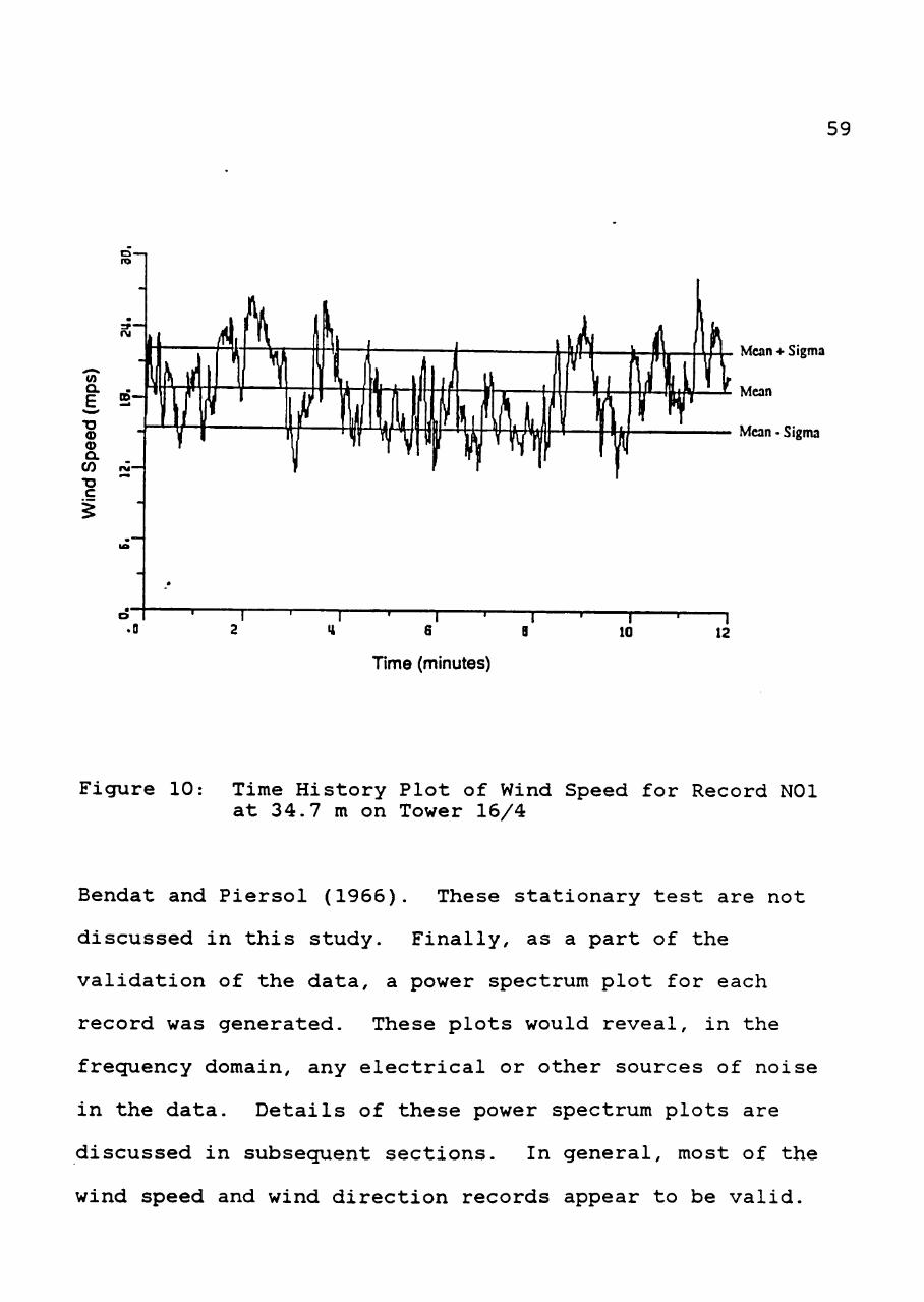
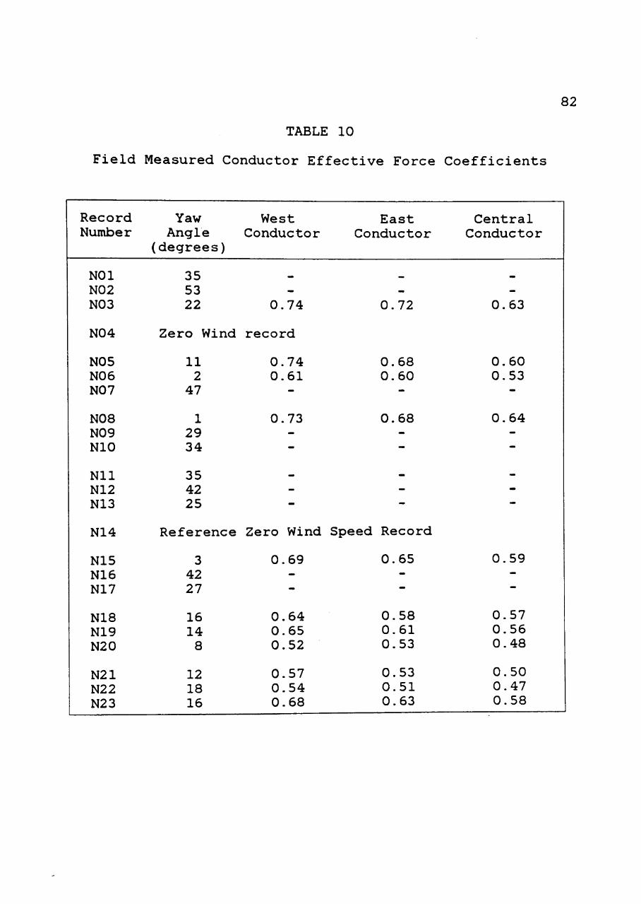
mean response of the west conductor is larger than that for
the east conductor as discussed in the previous section (see
Table 9).
There are three possible reasons for the scatter in the
values of effective force coefficient. The first reason may
be the accuracy with which transverse loads are measured.
Field measured transverse load components could vary by
about 10%, (see the previous section on validity of
conductor response data). The second reason may be the
modification of the wind speed for different heights above
the ground. In calculating the effective height of each
conductor, the conductor shape is assumed to be parabolic
and the site topography is taken into account. More
specifically, each effective height is calculated as the
average of the vertical distances between the ground and the
conductor at all points along the half spans on both sides.
The resulting values are 15.7 m for the east and west
conductors, and 23.8 m for the central conductor. The wind
profile is taken as having the same properties with respect
to the ground no matter how the ground elevation varies.
This raises some uncertainties, especially with regard to
the valley shown between Towers 16/4 and 16/5 in Figure 9.
Wind speeds are modified from the 34.7 m height to the 23.8
m effective height for the central conductor and to 15.7 m
84
effective height for west and east conductors using a wind
profile exponent value of a = 0.14. The modification in
wind speed is smaller for the central conductor than for the
west and east conductors. This could be the reason for the
force coefficients for the central conductor being smaller
than for the west and east conductors (refer to Table 10).
The third reason may be the wind characteristics of
turbulence and fluctuations in wind direction. As shown in
Table 5, many records show RMS of wind direction
fluctuations to be in the neighborhood of ten degrees.
These data in Table 5 suggest that the wind direction may
have fluctuated as much as 40 degrees within a record. In
addition, the turbulence intensity values shown in Table 8
are different between the records. Wind characteristics may
have significant effects on effective force coefficients.
The values of effective force coefficient obtained from
the field data are fairly consistent with the values shown
in Figure 3. The Reynolds Number for the field data is in
4 4 the range of 3x10 to 6x10 . For this range of Reynolds Number, Figure 3 suggest effective force coefficients in the
neighborhood of 0.6.
85
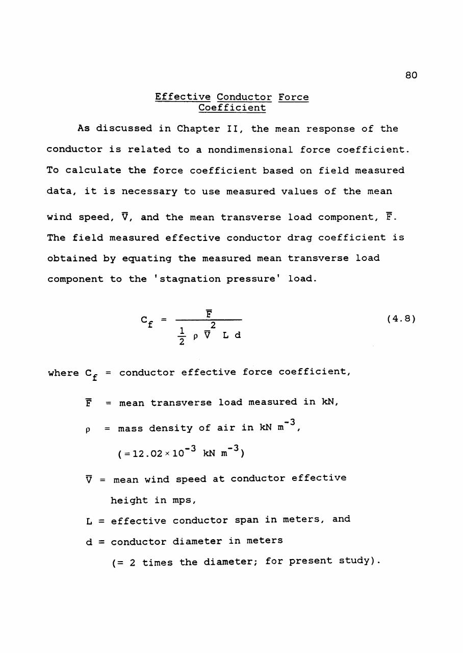
Response Spectrum
The conductor response spectrum represents the
fluctuating response about the mean response in the
frecjuency domain. Response spectra of west, east, and
central conductors for all records were obtained. A typical
response spectrum for the west conductor for record NOl is
shown in Figure 15. The response spectra were obtained
using the same procedure as for the gust spectra discussed
earlier. Similar to the gust spectra, the lower and upper
limits of the frecjuency range in spectral calculation are
0.0025 and 5 Hz, respectively. The response spectrum in
Figure 15 shows fluctuations in frecjuencies below 1 Hz, but
does not show a spike at a specific frecjuency. The range of
frecjuencies of interest for the present study is based on
natural frecjuencies of conductor vibration. The conductor's
natural frecjuencies are in the range of 0.1-0.4 Hz,
depending on its configuration. At frecjuencies between 2
and 4 Hz, the spectrum shows several very high peaks. These
peaks in the figure are somewhat misleading because the
spectral density function in the plot is multiplied by the
frecjuency. Generally, the spectral density function is
multiplied by frecjuency to get enhanced results in the
higher frecjuency ranges.
86
a CO O teiH
CO " » O >»,' CO
« V M
1
O 3 •3 >
1 ii CU
CO
Q 3 *
a
n CD
• a
o CM
• O
o .—1
f
o
a o
G.OOL
f - Frequency (in Hertz) S(f) - Spectral Density at f SIGSQ - Mean Sqaure Value
Zone Zone
^^Vr-n.. O . l
Frequenc:y, f (Hertz)
l . O
Zone III
Figure 15: Response Spectrum Plot for West Conductor Response for Record NOl
As noted in Chapter II, the area under the response
spectrum gives the mean scjuare of response. The response
spectrum is viewed in terms of area representing extent of
response. Peaks in the spectrum represent response at
specific frecjuencies. In order to discuss background and
resonant response, the spectrum is divided into three zones
for determination of relative response: (1) frequencies
87
less than 0.1 Hz, (2) frequencies between 0.1 Hz and 1.0 Hz,
and (3) frequencies greater than 1 Hz. Each zone of the
spectrum is reviewed in light of the conductor response to
wind.
The spectral area in the zone of frecjuencies less than
0.1 Hz is in the neighborhood of 75% for all records. This
response is primarily due to the background turbulence where
wind has significant turbulent energy (see Figure 13). The
peaks in the spectra in this zone do not represent dynamic
amplification of the response.
The spectral area in the zone between frecjuencies of
0.1 and 1.0 Hz is close to 15% for all records. Fundamental
transverse frecjuency of the conductor, f , in Hz for a
parabolic profile can be obtained using ecjuation 2.27. The
conductor sag depends on conductor span, horizontal tension
and temperature. The conductor span on the south side of
the Tower 16/4 is 450 m and toward the north it is 252 m
(see Figure 9). The sags, calculated using conductor
horizontal tension of 45 kN at 60°F, are 6.3 m and 21.0 m
corresponding to the 252 m and 450 m spans, respectively (a
parabolic profile is assumed). Using ecjuation 2.27 with
estimated sags, the calculated natural frecjuencies in the
transverse direction are 0.12 Hz and 0.22 Hz. The spectrum
in Figure 15 shows small but distinguishable peaks in the
88
neighborhood of these frequencies. The two unequal spans
are expected to respond in the transverse direction
independent of each other due to the low stiffness of the
conductor. The two peaks are judged to be due to resonant
response at natural transverse frecjuencies of the conductor.
At frecjuencies close to the conductor natural
frecjuencies the gust spectrum in Figure 13 shows that wind
has a fair amount of energy. Presence of gust energy at
natural frecjuencies of the conductor can cause significant
resonant amplification of the conductor response.
The spectral areas in the zone of frecjuencies greater
than 1 Hz are less than 15% in most of the records. High
spectral peaks (Figure 15) in the 2-4 Hz frecjuency range are
believed to be due to vibration of the tower and the
frecjuency of the swing angle indicators. These frecjuencies
of the tower and instruments enter into the conductor
response records since the conductor is connected to the
tower through load cells and swing angle indicators.
Natural frequencies of Tower 16/4 are determined using
MSC/NASTRAN version 63 software. The tower structure is
modelled as a space frame, without conductors and overhead
ground wires. Natural frecjuencies of the tower are 2.88,
3.01 and 4.92 Hz, corresponding to longitudinal, transverse,
and torsional modes of vibration, respectively. In
89
addition, the frequency of vibration of the swing angle
indicator is 3.2 Hz (Kempner, 1980). These frecjuencies of
the tower and the swing angle indicator are believed to
cause high peaks in the response spectrum in the frecjuency
range of 2 to 4 Hz. Even though spectral peaks are high in
the frecjuency range above 1 Hz, the amount of energy is
relatively low.
Since the amount of gust spectral energy above 1 Hz in
Figure 13 is very small and since peaks in the response
spectra can be justified as above, it is believed that the
response spectral energy in the frecjuency range above 1 Hz
is not due to response of the conductor to wind. This
spectral energy is neglected in further consideration of the
response of the conductors. The background and resonant
responses assessed from the response spectra are compared
with the analytical procedure in the next chapter.
CHAPTER V
COMPARISON AND REFINEMENT OF THE
ANALYTICAL MODEL
The goal of the present study is to compare and to
refine the analytical model using the results of field data.
The analytical model proposed by Davenport (1980) to
determine peak response of transmission line structures was
presented in Chapter II. The key elements in determining
the fluctuating response of conductors in the model are the
background response and the resonant response (see ecjuation
2.23). In addition, the model recjuires establishment a
value for the peak factor to determine peak response (see
ecjuation 2.1).
The field data analysis yields the peak response as
well as the fluctuating response. Background and resonant
responses are determined from response spectra of field data
utilizing the procedure indicated in Chapter IV. Peak
factors are obtained from the field peak responses utilizing
the upcrossing rate procedure.
Background and resonant responses assessed from the
field data are compared with values calculated using the
analytical model. Joint acceptance function coefficients
90
91
are obtained from the field data to refine the background
response of the analytical model. Also, aerodynamic damping
ratios are recovered from the field data to improve the
resonant response of the analytical model. Since the
fluctuating response depends on many parameters, total
fluctuating responses from field data are not compared with
total fluctuating response predicted using the Davenport
model (1980).
Comparison of Analytically Predicted Mean Square Response With Field
Measured Values
One of the two parts of the fluctuating response
component in ecjuation 2.1 is the mean scjuare value. In the
frecjuency domain analysis, the mean scjuare value of response
is computed as the area under the response spectrum. The
mean scjuare value can be considered as a summation of
background response, B , and resonant response, R (ecjuation
2.23). Background response is due to the wind turbulence at
low frecjuencies, and can be considered as quasi-static
response. Resonant response is due to coincidence of
conductor natural frecjuencies with gust frecjuencies. This
resonant response is the area under the response spectrum at
frecjuencies close to conductor natural frecjuencies.
92
Field Measured Mean Scjuare Response
The gust spectrum of Figure 13 shows that the wind
turbulence has energy up to 1 Hz, and energy beyond 1 Hz is
negligible. Conductor natural frecjuencies are in the range
of 0.1 to 0.4 Hz, hence the resonant peaks should dominate
above the background response in this frecjuency range. It
is difficult to separate background and resonant responses
in the field data. In Figure 16, which is the same response
spectrum as Figure 15, there are peaks at the natural
frecjuencies of the conductors: 0.12 and 0.22 Hz. However,
these peaks are diffused. As discussed in Chapter IV, the
spectral areas between the frecjuencies of 0.1 and 1.0 Hz for
most records were less than 15% of the total area under the
response spectrum (total mean scjuare value). At the risk of
being on the high side, the total spectral areas between
frecjuencies of 0.1 and 1.0 Hz are assumed to be resonant
response. The error introduced by this assumption is small
because the response in this frecjuency range is a small
portion of the total fluctuating response. This resonant
response is indicated by R in Figure 16.
It is reasonable to assume that the area under the
response spectrum below 0.1 Hz is the background response.
This area is close to 75% of the total area (total mean
scjuare value) in most of the records as discussed in Chapter
93
a 3* CJ
o en a
CO
O d CO
CO
«M CM
u o a •a > 1 a ° CO o
Q.OOL
f - Frequency (in Hertz) S(f) - Spectral Density at f SIGSQ - Mean Sqaure Value
0.1
Frequency, f (Hertz)
10.0
Figure 16: West Conductor Response Spectrum Plot for Record NOl
IV. The area designating background response is shown as B
in Figure 16.
The area under the response spectrum for frecjuencies
above 1 Hz is not considered to be response due to extreme
wind effects. This was discussed in some detail in Chapter
IV
94
Delineation of background and resonant responses in the
field response spectra permits assessment of responses in
each of the three conductors, west, east, and central
conductors, for all twenty-one field records. Field
measured values for background and resonant responses for
west, east, and central conductors are tabulated in Tables
11 through 13, along with mean scjuare values, for each
conductor. These values are compared with values predicted
by the analytical model as described in the next section.
The mean scjuare values of the three conductors are
fairly consistent, but have scatter for a given record.
This is not surprising, since there was variation (by about
10%) in the mean response of the three conductors (refer to
Table 9). It is reasonable to expect larger variation in
fluctuating response between the conductors. The variation
in the field data suggests that results will have scatter,
and that it is important to use an ensemble of data for
appropriate interpretation of the results.
Analytical Model Predicted Mean Scjuare Value
The analytical model used to predict the background and
resonant response contains a number of wind and conductor
related parameters (see ecjuations 2.24 and 2.25). These
parameters can be separated into fixed and variable
95
TABLE 11
West Conductor Response Spectrum Data Analysis
Record Number
NOl N02 N03
N04
N05 NO 6 N07
2 2
2 M
OO
O
vD
00
Nil N12 N13
N14
N15 N16 N17
N18 N19 N20
2 2
2 to
to
to
CA
) to
M
Mean Scjuare
0.211 0.184 0.043
Background Response
Field Analytical Measured Model*
0.141 0.132 0.028
Zero Wind Record
0.017 0.039 0.790
0.582 0.009 0.270
0.366 0.165 0.441
0.003 0.028 0.609
0.447 0.007 0.199
0.269 0.151 0.300
Reference Zero Wind
0.098 0.013 0.377
0.606 0.273 0.014
0.258 0.361 0.250
0.077 0.011 0.309
0.486 0.236 0.005
0.190 0.243 0.194
0.201 0.038 0.052
0.005 0.043 0.143
0.365 0.014 0.161
0.256 0.033 0.217
Resonant
Field Measured
0.033 0.024 0.009
0.008 0.006 0.087
0.057 0.001 0.037
0.043 0.010 0.077
Speed Record
0.069 0.005 0.152
0.186 0.125 0.002
0.076 0.151 0.177
0.015 0.002 0.041
0.066 0.024 0.002
0.042 0.060 0.036
. Response
Analytical Model*
0.254 0.043 0.056
0.006 0.048 0.203
0.502 0.012 0.200
0.348 0.034 0.288
0.077 0.004 0.192
0.259 0.140 0.003
0.095 0.194 0.194
* Davenport, 1980
96
TABLE 12
East Conductor Response Spectrum Data Analysis
Record Number
rH
CM
C
O
o o
o
2 2 2
N04
N05 NO 6 N07
2 2
2 M
OO
O
vD
00
Nil N12 N13
N14
N15 N16 N17
2 2
2 to
M M
O
VD
00
2 2
2 to
to
to
CA)
to M
Mean Scjuare
0.168 0.162 0.037
Background Response
Field Analytical Measured Model*
0.115 0.128 0.023
Zero Wind Record
0.009 0.033 0.677
0.572 0.013 0.207
0.310 0.165 0.348
0.002 0.021 0.541
0.450 0.009 0.157
0.231 0.153 0.248
Reference Zero Wind
0.078 0.020 0.321
0.512 0.205 0.008
0.193 0.276 0.187
0.059 0.017 0.268
0.420 0.178 0.002
0.147 0.199 0.153
0.181 0.037 0.050
0.004 0.041 0.141
0.322 0.015 0.155
0.245 0.037 0.195
Resonant Response
Field Measured
0.034 0.024 0.011
0.002 0.006 0.080
0.061 0.001 0.034
0.047 0.011 0.062
Speed Record
0.062 0.007 0.133
0.155 0.110 0.002
0.066 0.133 0.150
0.016 0.003 0.041
0.067 0.023 0.002
0.036 0.055 0.027
Analytical Model*
0.229 0.042 0.054
0.005 0.045 0.200
0.443 0.012 0.193
0.333 0.038 0.259
0.069 0.005 0.167
0.216 0.124 0.003
0.082 0.171 0.164
* Davenport, 1980
97
TABLE 13
Central Conductor Response Spectrum Data Analysis
Record Number
NOl N02 N03
NO 4
NO 5 NO 6 N07
NOB NO 9 NIO
Nil N12 N13
N14
N15 N16 N17
N18 N19 N20
N21 N22 N23
Mean Scjuare
0.284 0.183 0.040
Background Response
Field Analytical Measured
0.175 0.119 0.026
Zero Wind Record
0.011 0.047 1.004
0.618 0.020 0.287
0.432 0.148 0.471
0.004 0.036 0.714
0.467 0.009 0.206
0.294 0.136 0.308
Reference Zero Wind
0.117 0.014 0.443
0.638 0.300 0.019
0.320 0.420 0.269
0.094 0.012 0.365
0.524 0.261 0.005
0.236 0.271 0.210
Model*
0.211 0.035 0.053
0.005 0.043 0.147
0.391 0.015 0.163
0.269 0.035 0.222
Resonant
Field Measured
0.038 0.021 0.008
0.005 0.007 0.085
0.046 0.010 0.035
0.038 0.009 0.065
Speed Record
0.069 0.006 0.146
0.197 0.128 0.002
0.078 0.155 0.175
0.016 0.001 0.038
0.054 0.024 0.013
0.049 0.061 0.032
Response
Analytical Model*
0.207 0.031 0.044
0.004 0.037 0.162
0.417 0.009 0.158
0.283 0.028 0.228
0.060 0.004 0.142
0.212 0.111 0.002
0.076 0.155 0.148
* Davenport, 1980
98
parameters. Some of the parameters depend on the geometry
and physical characteristics of the conductors. These
parameters such as conductor sag, diameter of the conductor,
effective height, etc. are fixed parameters. On the other
hand, other parameters such as mean wind speed, turbulence
intensity and aerodynamic damping ratio vary with each wind
record; these parameters are considered as variable
parameters.
The fixed and assumed parameters used in the analytical
model to calculate background and resonant responses are
tabulated in Table 14. Each conductor bundle consists of
two Chukar conductors, hence the effective diameter used in
the model is twice the diameter of the individual conductor.
The mean wind speed at the effective conductor height is
determined using the recorded mean wind speed at 34.7 m and
the power-law exponent, a = 0.14.
Table 15 shows the mean wind speeds calculated for the
west, east, and central conductors at their effective
heights. The exposure factor, E, in ecjuations 2.24 and 2.25
is twice the turbulence intensity. The exposure factor
values in Table 15 are obtained from the turbulence
intensity recorded at 34.7 m on Tower 16/4 (refer to Table
7). The exposure factors used in the model at the effective
heights of the conductors are assumed to be the same as at
99
TABLE 14
Fixed and Assumed Parameters Used in the Analytical Model
Parameters Typical Values Used
0 . 0 8 m
376 m 402 m
15 .7 2 3 . 8
m m
Values based on physical characteristics
(1) Conductor diameter (d)
(2) Effective span (L) east and west conductors central conductor
(3) Effective height (h) east and west conductors central conductor
(4) Conductor fundamental frecjuency (f ) 0.12 Hz
Assumed values*
(5) Conductor force coefficient (C^) 1.0
(6) Coherence exponent (c) 8
(7) Scale of turbulence (L ) 65 m ^ ' s
(8) Kaimal's gust spectrum constant (A) 0.28
(9) Kaimal's gust spectrum constant (n) 0.67
*assumed values are recommended by Davenport (1980)
34.7 m on Tower 16/4. The conductor aerodynamic damping
ratio is calculated using ecjuation 2.26. Since the
aerodynamic damping ratio depends on the mean wind speed, it
is different for each record.
100
TABLE 15
Variable Parameters Used in the Analytical Model
Record Number
NOl N02 N03
N04 Ze
Exposure Factor
0.36 0.34 0.22
ro Wind Rec<
Mean
@ 15.7
16.9 14.7 13.3
ord
Wind
m*
Speed (mps)
@ 23.8 m**
17.9 15.5 14.1
N05 NO 6 NO 7
222
MOO
O v
D 00
Nil N12 N13
N14
N15 N16 N17
2 2 2
to M M
O V
D 00
2 2 2
to to to
CO to M
0.06 0.22 0.32
0.28 0.26 0.34
0.36 0.34 0.30
Reference
0.24 0.24 0.28
0.22 0.34 0.04
0.22 0.30 0.42
14.2 13.9 20.1
19.3 8.6 16.6
18.9 12.6 18.2
Zero Wind Speed Record
14.1 9.0 16.9
19.6 14.2 16.6
16.6 17.3 13.6
15.0 14.7 21.2
20.4 9.1 17.5
19.9 13.2 19.2
14.9 9.5 17.8
20.7 15.0 17.5
17.5 18.3 14.4
* effective height for west and east conductors ** effective height for central conductor
101
Instead of calculating the mean wind pressure, P, and
the influence coefficient, 0 (which translates the pressure
to response), the field measured mean transverse load
components are used for each record (refer to Table 9).
Calculated background and resonant responses using the
analytical model are shown for the three conductors in
Tables 11 through 13. The values are obtained using
ecjuations 2.24 and 2.25. The majority of the records show
that the background response calculated from the analytical
model is smaller than the background response measured in
the field. Field measured values versus analytical model
values of background response of the three conductors are
plotted in Figure 17. The figure shows that the background
response predicted by the model is an underestimation of the
measured value. Since the background response accounts for
75% of the mean scjuare response value, refinement of the
analytical model of this part is desirable.
The analytical model predicts higher resonant responses
than the field measured values (refer to Tables 11 to 13).
Field measured values versus analytical model values of
resonant response of the three conductors are plotted in
Figure 18. The figure clearly shows that the predicted
values are very much higher than the field measured values.
One of the significant variables in the analytical model is
102
0.8
U
s •a >
•a
•a
o West Cond. East Cond. Central Cond
0.6-
0.4-
1 1 * r—
0.4 0.6
Field Measured Values
0.8
Figure 17: Analytical Model Background Response Versus Field Measured Background Response
the aerodynamic damping ratio. If the damping ratio is
higher than predicted by equation 2.26, the calculated
resonant response will be smaller. Field measured data are
used to assess a possible damping ratio for each record.
103
Even though a large scatter in evaluation of the damping
ratio is expected, it can lead to a better prediction of
resonant response.
0.60
(/)
3 •a >
•a o •a c <
0.45-
0.30-
0.15-
0.00
Q
• •
•
B a
• ° y Q n /
a • /
- s°" v y v n / y y^
Q / y y^ a ^9 /yy
\™ 1
" /
1
V
Q
a •
V
West Cond. East Cond. Central Cond.
_ ,
0.00 0.15 0.30 0.45 0.60
Field Measured Values
Figure 18: Analytical Model Resonant Response Versus Field Measured Resonant Response
104
Refinement of the Analytical Model
As noted in previous sections, the analytical model
underestimates the background response and overestimates the
resonant response. Refinement of the analytical background
expression using the field measured data is attempted. The
resonant response prediction is improved by recovering a
damping ratio for the conductor from the field data.
Background Response
The mean scjuare value of fluctuating response can be
calculated as the area under the response spectrum,
al = J Sj (f) df (5.1) 0
2 where a„ = mean scjuare value of response,
So(f) = spectral density value of response, and
f = frecjuency.
Utilizing ecjuations 2.10 and 2.11, equation 5.1 can be
expressed as
_2 2 = iL- J y^^(f) |H(f)|2 S^(f) df (5.2)
- 0 V
where S (f) = gust spectral density,
F = mean transverse force,
V = mean wind speed.
105
2 Z (f) = aerodynamic admittance function, and
2 |H(f)| = mechanical admittance function.
The area under the response spectrum is a summation of
background and resonant responses. Ecjuation 5.2 can be
written in a simple form as:
_2 2 4F R = — T B ^ Aj,| (5.3)
V
where Ag accounts for background response, and A„ accounts
for resonant response. Davenport (1977) developed ecjuations
for Ag and Ap as
Ag = j x^(4r) S (f) ^ (5.4) 0 V
and
f L AR = X^(-^) S (f ) J |H(f)|^ df (5.5)
V 0
where f is the fundamental frecjuency of the structure and
other terms are defined above. The background response due
to wind turbulence can be obtained using ecjuations 5.3 and
5.4, if the gust spectrum is defined by some appropriate
analytical function.
The aerodynamic admittance function is a relationship
between the gust spectral density function and the force
106
spectral density function in the frequency domain. It is a
measure of the effect that the wind turbulence has on the
transverse forces. The shape of the conductor and the sizes
of gusts relative to the size of the conductor influence
this function. A large gust, totally enveloping the
structure, is well correlated, while a small gust, acting on
a portion of the conductor, is uncorrelated.
The aerodynamic admittance function is usually
2 f L expressed in a nondimensional form as x (- - )/ where L is V
the conductor span, and the ratio -F ^ designated as the
scale of turbulence (L ). The aerodynamic admittance
function is termed as a 'joint acceptance function (JAF),'
if it is modified to account for the mode shape. In other
words, the important link between the gust fluctuations,
(described by the gust spectrum) and the modal force
fluctuations is provided by the the JAF. This function
depends on the mode shape and the velocity field, which
varies widely from structure to structure. Davenport (1977)
reduced the JAF to a simple form as below:
|JAF|2 = -^—^ (5.6) ' ' 1 + m (p
where m is a constant to account for the mode shape and
107
<p = cfL/V. The quantities c, f, L, and V represent the
coherence exponent, frequency, conductor span and mean wind
speed, respectively.
The theory described for computing conductor response
in Chapter II is based on the conventional assumption of a
constant force coefficient. For conductors with a
cylindrical shape the force coefficient, C^, depends on the
Reynolds Number (refer to Figure 3). This change in force
coefficient affects the fluctuating component of response.
The analytical model of fluctuating response should account
for changes in the force coefficient at Reynolds Numbers
corresponding to the mean wind speed (Davenport, 1980). To
account for this effect the numerator of ecjuation 5.6 is
replaced with an unknown constant Q. The resluting
ecjuation, which is a product of JAF and Q is simply termed
as JAF in this study, as shown below:
|JAF|2 = 2 _ ^ _ . (5.7) 1 + M(-^)
V
In addition to introduction of coefficient Q in ecjuation
5.7, the coefficient M is used to account for mode shape and
the coherence exponent, c (transverse correlation of
turbulence). The available data are not able to provide
separate coefficients for the mode shape and correlation of
108
turbulence. Equation 5.7 is in the same form as equation
2.24 given in the analytical model developed by Davenport
(1980). In 1:he model, Davenport uses approximate values of
1 and 0.81 for the coefficients Q and M, respectively. Here
the field response data are used to evaluate these two JAF
coefficients.
Determinincr the JAF Coefficients
The frecjuency transfer function (FTF) is a transfer
function between the spectral densities of fluctuating wind
turbulence and conductor response. The FTF can be
considered as the product of the aerodynamic admittance
function and mechanical admittance function. The FTF can be
written as
^SR(f) v^ 2 2 5: 1-^- = 4 |H(f)r IJAFr. (5.8) _ 2 fS (f) I V /I I I V /
F
The FTF can be obtained by plotting the ratios of the
nondimensionalized response spectral values to the
nondimensionalized gust spectral values (refer to equation
5.8). As explained in Chapter IV, the IMSL program FTFREQ
is used to compute the spectral density values of wind
turbulence and conductor response fluctuations. FTF plots
for all 21 records of west, east, and central conductors
109
were obtained. A typical FTF plot for the west conductor
for record NOl is shown in Figure 19. The spectral density
values of wind turbulence above 1 Hz are very small (refer
to Figure 13), and use of very small values in the
denominator of the FTF would be inappropriate. Hence, the
FTF values are plotted up to 1 Hz only. It was noted in
Chapter IV that wind gust and response spectra show cjuite a
bit of fluctuation because of the computational procedures
used in obtaining the spectral densities. The FTF plot in
Figure 19 is obtained from the ratios of two spectra, so
large fluctuations in ordinates are not surprising.
The mechanical admittance function, also known as the
dynamic amplification factor, depends on the structural
dynamic properties such as frecjuencies and damping ratios.
This factor amplifies the response spectrum (resonant
response) at the natural frecjuencies of the conductor. The
JAF related to background response can be obtained by
removing the resonant peaks at the natural frecjuencies of
the conductor from the FTF plot. Equation 5.7 was fitted to
the field measured JAF plot by regression analysis to obtain
values of the coefficients Q and M. Equation 5.7 is a
nonlinear ecjuation, hence nonlinear regression needed to be
applied. The SAS procedure NLIN (SAS, 1982) was used to fit
the nonlinear equation to the computed JAF field response
110
28.0 -,
I I I I 1 1 1 1 '
0.001 10.0
Frequency (Hertz)
Figure 19: Frecjuency Transfer Function of West Conductor Response for Record NOl
data. The procedure NLIN is used to fit ecjuation 5.7 to the
field data of all 21 records of west, east, and central
conductors.
Procedure NLIN implements iterative methods that
attempt to find least squares estimates for the nonlinear
equations. Parameter names and starting values, expressions
for the model, and expressions for derivatives of the model
Ill
with respect to the parameters need to be specified. Based
on expectations, the specified ranges for the coefficients Q
and M were 0.4-1.0 and 0.1-0.4, respectively. The NLIN
procedure first examined the starting value specifications
of the parameters in the specified search grid. The NLIN
procedure then evaluated the residual sum of scjuares at each
combination of values to determine the best values to start
the iterative algorithm. A modified Gauss-Newton iterative
method (SAS, 1982) was used, which involved regressing the
residuals on the partial derivatives of the model with
respect to the parameters until the iterations converged.
Some variation in data was expected, since the data were
measured in the field.
To find the best coefficient values, which in general
satisfied most of the records, a contour of lowest residual
sum of scjuares was plotted in the specified search grid.
Any combination of coefficients Q and M within the lowest
residual sum of squares contour is acceptable. A typical
contour plot for west conductor response for record NOl is
shown in Figure 20. Combining all plots of three conductors
(west, east, and central), there are 63 contour plots of
residual sum of scjuares. The sixty three contour plots show
some degree of dispersion of lowest residual sum of scjuare
contours over the search grid. The contour plots were
112
e (J
i
0.1 0.2 0.3 0.4
Coefficient, M
Figure 20: West Conductor JAF Coefficients Contour Plot for Record N15
113
overlapped to find the best values of the coefficients Q and
M, which were 0.45 and 0.2, respectively. These values are
significantly lower than the values of 1.0 and 0.81 used in
tihe Davenport model (equation 2.24). For better
visualization the JAF with Davenport model values and
refined values are plotted on the same graph as shown in
Figure 21.
The low value of coefficient M obtained from the field
data may be because of a low value of coherence exponent, c,
due to the long span of the conductors. Also, when
-=- >> 1, the joint acceptance function is independent of ^s
the mode shape and is proportional to the ratio of the
correlation length to the conductor span. These comments
are based on the results of wind tunnel experiments
conducted on a rod (Blevins, 1977).
The expression for background response of the
conductor, ecjuation 2.24, with the new coefficients is
— ^ 2 2 B^ = P Ol E^
0.45
1 + 0.2(-^) ^s
(5.9)
The parameters in ecjuation 5.9 are defined below equation
2.24. The background response calculated using the refined
analytical model for all 21 records of west, east, and
central conductors are tabulated in Tables 16 through 18.
o CJ C
£ o c
o CJ
<
c 'o
o CM
O O o
o LT)
o o in
o
o o o -r 1 1 — I — I I M
0.001 0.0 ]
114
1 - Davenport Model 2 - Refined Model
- I 1 — I — r i l l -I 1 1—I—I I I "T 1 1—I—I I I I
0. 1.0 10.c
Reduced Frequency - fLA^
Figure 21: Joint Acceptance Function Plot
These tables also show the ratios of the refined analytical
model values to the field measured values and the ratios of
the analytical model values to the field measured values.
In general, these nondimensional ratios show a comparison
between the analytical model and the field response values.
For better visualization the field measured values versus
115
the refined analytical model values are plotted in Figure
22. The refined analytical model gave slightly better
predicted than the analytical model when Figures 22 and 17
are compared. In Tables 16 through 18, means and
coefficient of variations (COV) of the ensemble of the
ratios are shown. In each table, the mean of the ratio is
closer to 1 for the refined analytical model. However, the
COV for each conductor did not change. This improvement in
mean value of the ensemble and insignificant change in COV
value are due to inherent scatter in the field data.
Resonant Response
As noted earlier the analytical model overestimates the
resonant response. One of the reasons may be the use of low
damping ratio values as determined by ecjuation 2.26. Here
field measured resonant response data are used to estimate
damping ratios for the conductors.
Determining the Aerodynamic Damping
Ratio
As noted in Chapter II, three types of damping are
noted for conductor response, namely, material, structural,
and aerodynamic damping. For conductors aerodynamic damping
is very much higher than material or structural damping.
Therefore, both material and structural dampings are
TABLE 16
Background Response of West Conductor
116
Record Number
rH
CM
CO
O
O
O
22
2
N04
N05 NO 6 NO 7
22
2 M
OO
O
vD
00
Nil N12 N13
N14
N15 N16 N17
22
2 to
M M
O
VD
00
rH
CM
C
O
CM
CM
C
M
2 2 2
Mean Scjuare
0.211 0.184 0.043
Field Measured
0.141 0.132 0.028
Zero Wind Record
0.017 0.039 0.790
0.582 0.009 0.270
0.366 0.165 0.441
0.003 0.028 0.609
0.447 0.007 0.199
0.269 0.151 0.300
Reference Zero Wind
0.098 0.013 0.377
0.606 0.273 0.014
0.258 0.361 0.250
mean value coefficient of
0.077 0.011 0.309
0.486 0.236 0.005
0.190 0.243 0.194
variation
Refined Model
0.239 0.037 0.062
0.006 0.051 0.170
0.432 0.017 0.191
0.304 0.039 ,0.257
Speed Rec
0.082 0.006 0.180
0.220 0.148 0.003
0.090 0.179 0.210
Ratio (1)*
1.695 0.280 2.214
2.000 1.821 0.279
0.966 2.429 0.960
1.130 0.258 0.857
ord
1.065 0.546 0.583
0.453 0.627 0.600
0.474 0.739 1.083
1.003 65.5%
Ratio (2)*
1.426 0.288 1.857
1.667 1.536 0.235
0.817 2.000 0.809
0.952 0.219 0.723
0.896 0.455 0.492
0.383 0.530 0.400
0.400 0.621 0.912
0.839 65.3%
(1)* ratio of refined model value to the measured value (2)* ratio of analytical model value to the measured value
TABLE 17
Background Response of East Conductor
117
Record Number
NOl N02 N03
N04
Mean Scjuare
0.168 0.162 0.037
Field Measured
0.115 0.128 0.023
Zero Wind Record
Refined Model
0.215 0.043 0.060
Ratio (D*
1.870 0.336 2.609
Ratio (2)*
1.574 0.289 2.174
N05 NO 6 NO 7
N08 N09 NIC
Nil N12 N13
0.009 0.033 0.677
0.572 0.013 0.207
0.310 0.165 0.348
0.002 0.021 0.541
0.450 0.009 0.157
0.231 0.153 0.248
0.005 0.022 0.168
0.382 0.018 0.184
0.291 0.043 0.231
2.500 1.048 0.311
0.849 2.000 1.172
1.260 0.281 0.932
2.000 1.952 0.261
0.716 1.667 0.987
1.061 0.242 0.786
N14 Reference Zero Wind Speed Record
N15 N16 N17
N18 N19 N20
N21 N22 N23
mean
0.078 0.020 0.321
0.512 0.205 0.008
0.193 0.276 0.187
value coefficient of
0.059 0.017 0.268
0.420 0.178 0.002
0.147 0.199 0.153
variation
0.073 0.008 0.157
0.184 0.131 0.003
0.079 0.158 0.178
1.237 0.471 0.586
0.438 0.736 1.500
0.537 0.794 1.163
1.078 63.8%
1.051 0.412 0.496
0.369 0.618 1.000
0.449 0.668 0.980
0.940 64.3%
(1)* ratio of refined model value to the measured value (2)* ratio of analytical model value to the measured value
TABLE 18
Background Response of Central Conductor
118
Record Number
Mean Scjuare
Field Measured
Refined Model
Ratio (D*
NOl N02 N03
N04
NO 5 NO 6 NO 7
NOB N09 NIO
Nil N12 N13
N14
N15 N16 N17
N18 N19 N20
N21 N22 N23
0 .284 0 .183 0 .040
0 .175 0.119 0 .026
0 .256 0 .042 0 .064
1.463 0 .356 2 .462
Zero Wind Record
0.011 0.047 1.004
0.618 0.020 0.287
0.432 0.148 0.471
0.004 0.036 0.714
0.467 0.009 0.206
0.294 0.136 0.308
0.006 0.052 0.178
0.472 0.018 0.197
0.325 0.042 0.269
1.500 1.444 0.249
1.011 2.000 0.956
1.105 0.309 0.873
Reference Zero Wind Speed Record
0 .117 0 .014 0 .443
0 .638 0 .300 0 .019
0 .320 0 .420 0 .269
0 .094 0.012 0 .365
0 .524 0 .261 0.005
0 .236 0 .271 0.210
0 .083 0 .008 0 .176
0 .238 0 .155 0 .003
0 .095 0 .188 0 .211
0 .883 0 .667 0 .482
0 .454 0 .594 0 .600
0 .403 0 .694 1.005
mean value coefficient of variation
0.929 62.0%
Ratio (2)*
1.206 0 .294 2 .039
1.250 1.194 0 .206
0 .837 1.667 0 .791
0 .915 0 .257 0 .721
0 . 7 3 4 0 . 5 0 0 0 . 4 0 0
0.376 0 .490 0 .400
0 .331 0 .572 0 .833
0 .763 63.4%
(1)* ratio of refined model value to the measured value (2)* ratio of analytical model value to the measured value
119
0.8
_3
>
•s c
0.6-
0.4-
" West Cond. D East Cond. • Central Cond
0.2-
0.0 0.2 0.4 0.6 0.
Field Measured Values
Figure 22: Refined Model Background Response Versus Field Measured Values
neglected in this study, and the computed total damping is
assumed to be aerodynamic damping.
The response of the conductor at its natural frequency
of vibration is a function of excitation force and damping.
120
The magnification factor method is used here to estimate the
aerodynamic damping ratio. For a single degree of freedom
system subjected to wind turbulence, the resonant peak is
amplified at a fundamental frecjuency of the conductor. The
height of this peak is controlled by the damping for the
conductor.
The frecjuency transfer function (Figure 19) described
in the previous section is used to establish damping. As
noted earlier, the FTF is a combination of aerodynamic
admittance function and the mechanical admittance function.
The mechanical admittance function amplifies the response at
the natural frecjuency of vibration of the conductor. The
expression for the mechanical admittance function is defined
in ecjuation 2.13. At the fundamental frecjuency of the
conductor, the ecjuation for the mechanical admittance
function simplifies as follows:
|H(f^)|^ = - V (-^ 4 C
where C = aerodynamic damping ratio, and
f = fundamental frecjuency of conductor.
The damping ratios of the conductors are determined
using the heights of the resonant peaks in the FTF plots.
As noted in Chapter III, the conductor spans on two sides of
Tower 16/4 are different. The natural frecjuencies of
121
vibration of the conductors are 0.12 Hz and 0.22 Hz,
corresponding to spans of 450 m and 252 m, respectively.
The aerodynamic damping ratios estimated to be related to
these two natural frecjuencies of the west, east, and central
conductors from the FFT are tabulated in Table 19.
Conductor aerodynamic damping ratios for east wind records
(N05, N09 and N20) are not calculated because the peaks in
the FTF plots for these records are highly erratic. The
east wind records give poor results for the FTF because of
low turbulence intensities in tihe records. The estimated
aerodynamic damping ratios in Table 19 vary between 18 and
91%. This large scatter in establishing damping ratios is
expected because computational technicjues used to obtain the
spectra cause large fluctuations in FTF. In addition only
two specific peak values, closest to the frecjuencies of 0.12
and 0.22 Hz, are used in each FTF plot. The peak values in
the FTF plots are not expected to be highly accurate. Most
of the estimated damping values in Table 19 fall between 30%
and 60%.
The aerodynamic damping values predicted by ecjuation
2.26 are between 5% and 11% based on the mean winds recorded
in the field. These values used in the analytical model are
significantly smaller than the ones estimated from the field
data. In recognition of this discrepancy, a conservative
TABLE 19
122
Estimated Aerodynamic Damping Ratios in Percentages
Record Number
NOl N02 N03
N04
N05 NO 6 NO 7
NOB N09 NIO
Nil N12 N13
N14
N15 N16 N17
N18 N19 N20
N21 N22 N23
West Conductor (1)*
45 66 43
Zero Wind
_
50 18
52 -
34
32 50 39
Reference
50 88 47
33 42 -
45 58 58
(2)*
43 66 91
Record
_
30 33
35 -
38
58 52 67
Zero Wind
41 75 69
35 46 -
29 33 29
East Conductor (1)*
43 32 38
^
41 18
50 -
27
32 22 44
Speed
45 29 44
30 45 —
45 60 60
(2)*
41 34 67
^
32 33
35 -
45
58 54 60
Record
40 28 75
41 42 —
29 32 34
Central Conductor (1)*
46 27 62
^
65 47
55 —
30
38 28 47
50 50 54
37 54 —
41 56 67
(2)*
44 34 66
^
37 22
35 —
41
50 50 63
37 50 52
51 42 —
27 33 56
(1)* corresponding to (2)* corresponding to
resonant peak at 0.12 Hz resonant peak at 0.22 Hz
123
ensemble average value of 40% aerodynamic damping ratio is
suggested for conductors. Resonant responses are calculated
with this suggested aerodynamic damping for comparison
purposes.
Resonant Response with Suggested Damping Ratio
Resonant response values for all three (west, east, and
central) conductors are calculated using an aerodynamic
damping ratio of 40% in the analytical model. The values
are tabulated in Tables 20 through 22. The tables also show
the field measured resonant response and the total mean
scjuare value for each record.
In addition, ratios of resonant responses obtained from
the analytical model with 40% damping to field measured
values and from the analytical model with damping from
ecjuation 2.26 to field measured values are shown in the
tables. Use of 40% damping improves the prediction of
resonant response significantly. Mean values of the ratios
for 40% damping are close to unity. The COV of the ratios
in the tables are not effected significantly, though this is
misleading. The mean values of the ratios of responses from
the analytical model with damping from ecjuation 2.26 are a
little more than 4; hence associated COV values of 45%
reflect a large variation.
124
TABLE 20
West Conductor Resonant Response With 40% Damping
Record Number
NOl N02 N03
NO 4
NO 5 N06 NO 7
NOB N09 NIO
Nil N12 N13
N14
N15 N16 N17
N18 N19 N20
N21 N22 N23
Mean Scjuare
0.211 0.184 0.043
Zero Wind
0.017 0.039 0.790
0.582 0.009 0.270
0.366 0.165 0.441
Reference
0.098 0.013 0.377
0.606 0.273 0.014
0.258 0.361 0.250
mean value
Field Measured
0.033 0.024 0.009
Record
0.008 0.006 0.087
0.057 0.001 0.037
0.043 0.010 0.077
Zero Wind
0.015 0.002 0.041
0.066 0.024 0.002
0.042 0.060 0.036
coefficient of variation
Analytical Model
0.053 0.008 0.009
^
0.008 0.051
0.119 —
0.041
0.081 0.006 0.064
Speed Reco
0.014 0.001 0.039
0.062 0.025
-
0.019 0.042 0.033
Ratio (1)*
1.606 0.333 1.000
1.333 0.586
2.088 •
1.108
1.884 0.600 0.831
rd
0.933 0.500 0.950
0.939 1.042
-
0.452 0.700 0.917
0.989 48.5%
Ratio (2)*
7.697 1.792 6.222
8.000 2.333
8.807 .
5.405
8.093 3.400 3.740
5.133 2.000 4.683
3.924 5.833
-
2.262 3.233 5.389
4.886 45.8%
(1)* ratio of analytical model values with 40% damping ratio to the field measured values
(2)* ratio of analytical model values with damping ratio from ecjuation 2.26 to the field measured values
125
TABLE 21
East Conductor Resonant Response With 40% Damping
Record Number
NOl N02 N03
N04
N05 NO 6 N07
NOB N09 NIC
Nil N12 N13
N14
N15 N16 N17
N18 N19 N20
N21 N22 N23
Mean Scjuare
0.168 0.162 0.037
Zero Wind
0.009 0.033 0.677
0.572 0.013 0.207
0.310 0.165 0.348
Reference
0.078 0.020 0.321
0.512 0.205 0.008
0.193 0.276 0.187
mean value
Field Measured
0.034 0.024 0.011
Record
0.002 0.006 0.080
0.061 0.001 0.034
0.047 0.011 0.062
Zero Wind
0.016 0.003 0.041
0.067 0.023 0.002
0.036 0.055 0.027
coefficient of variation
Analytical Model
0.047 0.008 0.009
^
0.008 0.050
0.105 -
0.039
0.078 0.006 0.057
Ratio (1)*
1.382 0.333 0.818
.
1.333 0.625
1.721 •
1.147
1.660 0.550 0.919
Speed Record
0.012 0.001 0.035
0.052 0.022 -
0.017 0.036 0.027
0.750 0.333 0.854
0.776 0.957
-
0.472 0.665 1.000
0.905 45.4%
Ratio (2)*
6.735 1.750 4.909
7.500 2.500
7.262 _
5.676
7.085 3.455 4.177
4.313. 1.667 4.073
3.224 5.391
-
2.278 3.109 6.074
4.510 42.6%
(1)* ratio of analytical model values with 40% damping ratio to the field measured values
(2)* ratio of analytical model values with damping ratio from ecjuation 2.26 to the field measured values
126
TABLE 22
Central Conductor Resonant Response With 40% Damping
Record Number
rH
CM
CO
O
O O
2
2 2
N04
N05 NO 6 NO 7
22
2 M
OO
O
vD
00
Nil N12 N13
N14
N15 N16 N17
2 2
2 to
M M
O
VD
00
rH
CM
CO
CM
C
M
CM
2 2 2
Mean Scjuare
0.284 0.183 0.040
Field Measured
0.038 0.021 0.008
Zero Wind Record
0.011 0.047 1.004
0.618 0.020 0.287
0.432 0.148 0.471
0.005 0.007 0.085
0.046 0.010 0.035
0.038 0,009 0.065
Analytical Model
0.045 0.006 0.008
0.007 0.043
0.105
0.034
0.070 0.005 0.054
Reference Zero Wind Speed Rec
0.117 0.014 0.443
0.638 0.300 0.019
0.320 0.420 0.269
0.016 0.001 0.038
0.054 0.024 0.013
0.049 0.061 0.032
mean value coefficient of variation
0.011 0.001 0.032
0.054 0.020
0.017 0.035 0.026
Ratio (D*
1.184 0.286 1.000
1.000 0.506
2.283
0.971
1.842 0.556 0.831
ord
0.688 1.000 0.842
1.000 0.833
0.347 0.574 0.813
0.920 53.0%
Ratio (2)*
5.447 1.476 5.500
5.286 1.906
9.065
4.514
7.447 3.111 3.508
3.750 4.000 3.737
3.926 4.625
1.551 2.541 4.625
4.223 45.8%
(1)* ratio of analytical model values with 40% damping ratio to the field measured values
(2)* ratio of analytical model values with damping ratio from equation 2.26 to the field measured values
127
For better visualization, a plot of the resonant
response predicted by the analytical model with 40% damping
versus the field measured resonant values is shown in Figure
23. This figure, when compared with Figure 18, shows that
the analytical model predicted better resonant values with
40% aerodynamic damping ratio. Figure 23 also illustrates
the inherent scatter in the field data.
Peak Factors
Another important component of the analytical model for
fluctuating response is the peak factor, g. It is used to
predict the peak response value that can occur in a time
segment. The peak factor is defined as the number of root
mean scjuare values by which the peak value exceeds the mean
value. The peak factor for field measured response data is
calculated using the ecjuation
g = JLJL_R (5.11) ^R
where ft = peak response value,
R = mean response value, and
<Tp = root mean scjuare of response.
The peak factor values vary depending on the averaging
time interval; the smaller the peak averaging time interval
the higher the peak factor value. The peak factors from the
128
0.12
u 3 •a >
"8 :z "a u •c c
<
0.09-
• West Cond. a East Cond. • Central Cond
0.06-
0.03-
0.00 0.00 0.03 0.06 0.09 0.12
Field Measured Values
Figure 23: Analytical Model Resonant Response With 40% Damping Versus Field Measured Values
field data for response of the three conductors (west, east,
and central) are calculated and tabulated in Table 23.
The values computed are based on 0.1 and 1 second time
averaged peak values. As expected, peak factors calculated
129
TABLE 23
Peak Factors for Conductor Response
Record Number
NOl N02 N03
NO 4
West Conductor
5.62* 4.00** 3.97 3.03 4.54 3.94
Zero Wind Record
East Conductor
6.60 4.54 3.99 3.16 5.12 4.32
Central Conductor
6.91 3.26 5.37 2.69 5.53 4.54
N05 NO 6 NO 7
NOB N09 NIC
Nil N12 N13
4.77 4.07 5.14
3.48 3.28 4.29
6.67 3.76 5.45
2.07 3.30 3.20
2.74 2.88 3.34
4.52 3.60 4.20
4.18 4.02 3.74
3.42 3.30 4.33
6.78 3.37 7.09
2.31 3.00 3.12
2.72 2.73 3.38
5.11 3.15 4.69
3.71 4.75 6.40
3.59 3.52 4.32
6.06 3.95 4.45
2.80 4.28 3.04
2.52 3.07 3.43
4.02 3.58 3.36
N14
N15 N16 N17
NIB N19 N20
N21 N22 N23
Reference Zero Wind Speed Record
* based on 0.1 second peak values (instant peaks) ** based on 1 second average peak values
4.15 3.88 5.68
3.89 4.01 3.75
4.02 5.62 3.32
3.75 3.69 4.61
3.18 3.52 2.01
3.29 4.43 2.42
4.65 3.69 5.71
4.19 4.63 4.37
4.83 5.99 3.16
3.85 3.34 4.90
3.05 3.88 2.15
3.85 5.01 2.51
4.76 4.12 4.67
3.94 4.41 4.02
4.01 4.10 4.09
3.81 3.68 3.86
3.13 3.51 3.04
3.27 3.34 2.47
130
for 0.1 second peaks are higher than those calculated for 1
second time average. The peak factors for 0.1 second time
averages range between 3.16 and 6.78, and for 1 second time
averages they range between 2.01 and 5.11. The suggested
range for peak factors in the analytical model is 3.5 to 4.0
(Davenport, 1980). Many records show that the peak factors
measured in the field are higher than 4.0. This is not
surprising in view of the fact that wind speed fluctuations
tend to be Gaussian, while the response fluctuations
associated with flow separation are often highly
intermittent, thus giving rise to large peak factors. The
peak factors vary from record to record and their
distribution functions are recjuired in order to establish
peak values with a specified probability of being exceeded.
Peak factors as function of the probability distribution of
upcrossings, or ecjuivalently, a specified number of
occurrences in a given interval of time, are obtained from
the field data.
Probabilistic Peak Factors from Field Data
For a stationary Gaussian process the cumulative
probability distribution in terms of upcrossings can be
stated as (refer to ecjuation 2.21).
131
2 P(>x) = exp - { - ^ 1 (5.12)
2 G^ X
where P(>x) = probability of upcrossing.
X - threshold level specified (=gCT ), and
CT - root mean scjuare.
The Rayleigh distribution function in ecjuation 5.12 can
be expressed in Weibull distribution form as
k P(>x) = exp -(-2.) (5.13)
where g = X /
and c , k = c o n s t a n t s .
Ecjuation 5 .13 can be expanded as
I n ( - I n P(>x) ) = k l n ( g ) - k l n ( c ) . ( 5 . 1 4 )
A graph of P(>x) versus x on an appropriate log scale
will yield k as the slope of the straight line and c as the
zero intercept.
Upcrossing rates were calculated for different
threshold values (multiples of RMS) of response of all three
conductors for each record. The field data used were the
0.1 second time interval responses. A linear regression
line was fitted for each record to assess trends with
132
respect to wind speed, wind direction, and turbulence
intensity. The conductor response data did not indicate any
specific trend for wind speed, wind direction or turbulence
intensity (terrain roughness). The upcrossing rates for
eighteen west wind records are plotted on the same graph, as
shown in Figure 24. Even though values have scatter, there
is a specific trend. A linear regression line is fitted to
the ensemble of data, as shown in Figure 24. The regression
line has a correlation coefficient of 0.93. This
correlation coefficient lends credence to the use of data as
an ensemble. Values for k and c in ecjuation 5.14 are 0.580
and 0.136, respectively.
For the Rayleigh distribution, values of k and c are 2
and 1.414, respectively. A line representing a Rayleigh
distribution is shown in Figure 24. The regression line
fitted to the field data is quite different from the
Rayleigh distribution line, indicating that the conductor
response data has a non-Gaussian distribution. It is
observed in Figure 24, that a Rayleigh distribution
underestimates upcrossing rate as compared to the field
data. The upcrossing rate plot can be used to determine the
peak factor for a desirable probability of upcrossings. The
peak factors obtained from the plot are based on 0.1 second
peak values.
133
0.000000001 T
0.000005 •
o JO CO CO
9 D "o ! »
(0 n p
0.0006
0.0111 r
0.066"
A
0.2
0.4
1.7 2.7 4.5 7.4
Peak Factor, g
Figure 24: Cumulative P r o b a b i l i t y D i s t r i b u t i o n of Upcross ings for Conductor Response
CHAPTER VI
CONCLUSIONS
The purpose of this study was to compare and refine the
analytical model to predict dynamic responses of electrical
transmission line conductors to extreme winds using field
data. Wind and conductor response field data were obtained
from a full-scale field experiment. The field data were
collected by the Bonneville Power Administration (BPA) from
an instrumented single circuit 500 kV lattice tower on the
John Day-Grizzly line 2, which is located at the Moro site
in northern Oregon. The conductor spans 252 m and 450 m on
two sides of the instrumented tower. A total of
twenty-three twelve-minute duration records were utilized in
thi s study.
Based on the analysis of field data and the refinement
of the analytical model originally developed by Davenport
(1980), the following conclusions are made:
(1) The field measured wind and conductor response data
were found to be valid. The mean -responses of three
conductors were within 10% of each other for all
records. Fluctuating responses of the conductors
showed a significant amount of scatter.
134
135
(2) Winds traversing over the valley showed a wide
variation in profile and turbulence. Winds coming from
similar terrains of valleys and hills have a power-law
exponent range from 0.11 to 0.18 and a turbulence
intensity range from 0.11 to 0.21.
(3) The wind spectra showed 99% of spectral energy in the
frecjuency range below 1 Hz. The amplitude constant A
for Kaimal's gust spectrum was found to be within the
suggested range of 0.15 to 0.60; however, the exponent
constant n from the field data was much higher than the
suggested range of 0.33 to 0.67.
(4) The field measured effective conductor force
coefficient was found to vary between 0.48 and 0.75.
(5) Noticeable resonant peaks occurred in the frecjuency
range from 0.1 to 0.4 Hz. in the conductor response
spectra. Two of these peaks close to 0.12 and 0.22 Hz
were identified as corresponding to natural transverse
frecjuencies of the conductors associated with the two
unecjual spans. The resonant response energy level was
found to be low, less than 15% of the total energy in
most records.
(6) The majority of the records showed that the field
measured background turbulence response of the
conductors accounted for 75% of the fluctuating
response.
136
(7) The analytical model for background response was
refined by determining the joint acceptance function
(JAF) coefficients from the field measured data. The
best values for the coefficients (ecjuation 5.7) are
judged to be Q=0.45 and M=0.20.
(8) Damping of the conductors, found from the field
measured data, was much higher than the theoretical
aerodynamic damping ratio. A damping value of 40% is
suggested for the conductors.
(9) The refinement of JAF coefficients and use of
aerodynamic damping factor of 40% in the analytical
model gave a significant improvement in prediction of
background and resonant responses when results were
compared with the field measured data. However, ratios
of refined analytical model values to field measured
values showed a large scatter.
(10) Many records showed response peak factors (for 0.1
second response) to be higher than the range of 3.5-4.0
suggested in the analytical model. The upcrossing rate
principle was used to determine the peak factors on a
probabilistic basis. The Weibull distribution
satisfactorily describes the probability distribution
of the upcrossings rate.
137
It is recommended that additional field data be
obtained, particularly at reasonably predictable sites, to
further verify and refine the analytical model. The
computational procedures presented here are general and are
applicable to additional field data.
REFERENCES
ANSI, 1982: "Minimum Design Loads for Building and Other Structures, ANSI 58.1-1982," American National Standards Institute, Inc., ANSI, New York, NY.
ASCE, 1984: "Guidelines for Transmission Line Structural Loading," American Society of Civil Engineers, New York, NY.
Bendat, J.S., and Piersol, A.G., 1966: "Measurements and Analysis of Random Data," John Wiley and Sons, Inc., New York, NY.
Bendat, J.S., and Piersol, A.G., 1980: "Engineering Applications of Correlation and Spectral Analysis," John Wiley and Sons, Inc., New York, NY.
Blevins, R.D., 1977: "Flow-Induced Vibration," Von Nostrand Reinhold Company, New York, NY.
Brunt,. S.D., 1952: "Physical and Dynamical Meteorology," Second Edition, Cambridge University Press, England.
Chatfield, C , 1975: "The Analysis of Time Series: Theory and Practice," Chapman and Hall, London.
Criswell, M.E., and Vanderbilt, M.D., 1987: "Reliability-Based Design of Transmission Line Structures: Final Report," EPRI EL-4793, Project 1352-2, Vol. I, EPRI, Palo Alto, California, March.
Davenport, A.G., 1960: "Wind Loads on Structures," Technical paper No. 88 of the Division of Building Research, National Research Council of Canada, March.
Davenport, A.G., 1961: "The Application of Statistical Concepts to the Wind Loading of Structures," Proceedings of Institute of Civil Engineers, Vol. 19, pp. 449-471, August.
Davenport, A.G., 1967: "Gust Loading Factors," Journal of the Structural Division, Vol. 93, ST3, ASCE, New York, NY, pp. 11-34, June.
138
139
Davenport, A.G., 1972: "Approaches to the Design of Tall Buildings Against Wind," Theme Report, Proceedings of the ASCE-IABSE International Conference on Planning and Design of Tall Buildings, Lehigh University, pp. 1-22, August.
Davenport, A.G., 1977: "The Prediction of the Response of Structures to Gusty Wind," Proceedings of International Research Seminar, Safety of Structures Under Dynamic Loading, Vol. I, Norwegian Institute of Technology, Trondheim, Norway, pp. 257-284, June.
Davenport, A.G., 1980: "Gust Response Factors for Transmission Line Loading." Wind Engineering, Proc. of the Fifth International Conference on Wind Engineering, J.E. Cermak, Ed. (Fort Collins, CO; July 1979), Pergamon Press, New York, NY.
Ferraro, V., 1983: "Transverse Response of Transmission Lines to Turbulent Winds." Masters Thesis, The University of Western Ontario, London, Ontario, Canada, July.
GAI Consultants, Inc., 1981: "Transmission Line Wind Loading Research," EPRI Interim Report, RP 1277, EPRI, Palo Alto, California, April.
Ghiocel, D., and Lungu, D., 1975: "Wind Snow and Temperature Effects on Structures based on Probability," Abacus Press, Kent, England.
Gould, P.L., and Abu-Sitta, S.H., 1980: "Dynamic Response of Structures to Wind and Earthcjuake Loading, " John Wiley and Sons, Inc., New York, NY.
IMSL, 1982: International Mathematical and Statistical Libraries, Inc., Vol. 2.
Jan, Con-Lin, 1982: "Analysis of Data for the Response of Full-Scale Transmission Tower Systems Real Winds," Masters thesis, Texas Tech University, Lubbock, Texas, December.
Jenkins, G.M, and Watts, D.G., 1968: "Spectral Analysis and its Applications," Holden-Day, San Fransisco, California.
Kaimal, J.C, 1978: "Horizontal Velocity Spectra in an Unstable Surface Layer," Journal of the Atmospheric Sciences, Vol. 35, pp. 18-24.
140
Kancharla, V.S., 1987: "Analysis of Wind Characteristics from Field Wind Data," Masters thesis, Texas Tech University, Lubbock, Texas, May.
Kempner, L., Jr., 1979: "Wind Loading on a Latticed Transmission Tower," Report No. ETKA-79-1, Bonneville Power Administration, U.S. Dept. of Energy, November.
Kempner, L., Jr., and Laursen, H.I., 1977: "Response of a Latticed Transmission Tower," Report No. ETB-77-1, Bonneville Power Administration, U.S. Dept. of Energy, November.
Kempner, L., Jr., and Laursen, H.I., 1981: "Measured Dynamic Response of a Latticed Transmission Tower and Conductors to Wind Loading," Report No. ME-81-2, Bonneville Power Administration, U.S. Dept. of Energy, July.
Kempner, L., Jr., and Thorkildson, R.M., 1982: "Moro Test Site Wind Parameter Study." Report No. ME-82-3, Bonneville Power Administration, U.S. Dept. of Energy, December.
Kempner, L., Jr., Volpe, H.W., and Thorkildson, R.M., 1985: "Wind Loading Research on Transmission Line," Proceedings of the Fifth International Conference on Wind Engineering, Texas Tech University, Lubbock, Texas, November.
Kim, Soo-Il, 1977: "Wind Loads on Flat Roof Area Through Full-Scale Experiment," Doctoral Dissertation, Texas Tech University, Lubbock, Texas.
Mehta, K.C., Norville, H.S., and Kempner, L., Jr., 1986: "Electric Transmission Structure Response to Wind," Proc. International Symposium on Probabilistic Methods Applied to Electric Power Systems, Samy Krishnasamy, Ed., (Ontario Hydro, Toronto, Canada; July 1986), Pergamon Press, New York, NY.
141
Melbourne, W.H., 1975: "Peak Factors for Structures Oscillating Under Wind Action." Proc, Fourth International Conference on Wind Effects on Buildings and Structures, Cambridge University Press, London, England.
Miller, I., and Freund, J.E., 1977: "Probability and Statistics for Engineers," Second ed., Prentice-Hall, Inc., Englewood Cliffs, New Jersey.
NESC, 1984: "National Electric Safety Code," ANSI C2, Institute of Electrical and Electronics Engineers, Inc., Wiley-Interscience, New York, NY.
Nigam, N.C., 1983: "Introduction to Random Vibrations," The MIT Press, Cambridge, Massachusetts, London, England.
Norville, H. S., K.C. Mehta, andA.F. Farwagi, 1985: "500 kV Transmission Tower/Conductor Wind Response: phase I," Institute for Disaster Research, Texas Tech University, Lubbock, Texas, May.
NRCC, 1980: "National Building Code of Canada," NRCC No. 17724, Associate Committee on the National Building Code, National Research Council of Canada, Ottawa, Canada.
Potter, J.L., and Boylan, D.E. 1981: "Aerodynamic Force Coefficients for the Prediction of Wind Loads on Electrical Transmission Lines," Sverdrup Corporation, Report submitted to EPRI, Palo Alto, California.
Pries, R.A., 1981: "Moro 1200 kV Structural/Mechanical Test Program," Report No. ME-81-1, Bonneville Power Administration, U.S. Dept. of Energy, March.
Racicot, R.L., 1969: "Random Vibration Analysis-Application to Wind Loaded Structures," Report No. 30, School of Engineering, Case Western Reserve University, Cleveland, Ohio, February.
Rice, S.O., 1945: "Mathematical Analysis of Random Noise," Bell System Technical Journal, Vol. 24, pp. 46-156.
Sachs, P., 1978: "Wind Forces in Engineering," Second Edition, Pergamon Press, New York.
Simiu, E., and Scanlan, R.H., 1985: "Wind Effects on Structures: An Introduction to Wind Engineering," John Wiley and Sons, Inc., New York, NY.
142
Statistical Analysis System (SAS), 1985: "SAS User Guide: Statistics," SAS Institute, Inc., Gary, North Carolina.