Response of the bottom boundary layer over a sloping shelf to

variations in alongshore wind

A. Perlin, J. N. Moum, and J. M. Klymak1

College of Oceanic and Atmospheric Sciences, Oregon State University, Corvallis, Oregon, USA

Received 20 May 2004; revised 22 October 2004; accepted 30 December 2004; published 14 September 2005.

[1] Rapidly repeated transects of currents, density, and turbulence through the bottomboundary layer across a relatively uniform stretch of the continental shelf off Oregonreveal the response to a sequence of strong upwelling followed by relaxation and thence aresumption of upwelling. Several definitions of boundary layer thickness are employedto describe the evolution of the bottom boundary layer. Well-mixed and turbulent layerswere typically confined to 10 m from the bottom. However, boundary layer thicknesseswere greatest during relaxation from upwelling (when mixed layer and turbulent layerthicknesses exceeded 20 m), and turbulence in the bottom boundary layer was mostintense at this time. Dense, near-bottom fluid was observed to move upslope withupwelling and back down the slope with relaxation from upwelling. By tracking theintersection of near-bottom isopycnals with the bottom over successive transects, weestimate the cross-shore speed of fluid in the bottom boundary layer. Cross-shore speedagrees well with dynamical estimates of cross-shore velocity in the bottom Ekman layerderived from bottom stress measurements. This leads to a confirmation of the Ekmanbalance of alongshore momentum in the bottom boundary layer across the full width of theshelf. Good correlation exists between alongshore velocity at the top of the bottomboundary layer and cross-shore velocity of dense fluid in the bottom boundary layer.Application of a derived proxy for bottom stress to moored velocity observations indicatesEkman balance of alongshore momentum at a midshelf location (81 m depth) for a 3 monthperiod in spring/summer 2001.

Citation: Perlin, A., J. N. Moum, and J. M. Klymak (2005), Response of the bottom boundary layer over a sloping shelf to variations

in alongshore wind, J. Geophys. Res., 110, C10S09, doi:10.1029/2004JC002500.

1. Introduction

[2] Cross-shelf circulation in coastal upwelling regions isdetermined to a great extent by flows in the surface andbottom boundary layers (BBL). Wind forcing generatescross-shore motion of water in the surface Ekman layer.This, in turn, creates a pressure gradient which drivesalongshore flow beneath the surface layer. A consequenceof this alongshore flow is a near-bottom Ekman transportopposite in direction to that in the surface layer.[3] It has proven to be quite difficult to obtain clear

observations of cross-shore motion in the BBL. Mooredvelocity measurements in the BBL have indicated thecomplexity of the temporal structure of the BBL [Weatherly,1972; Mercado and van Leer, 1976; Kundu, 1976; Dickeyand van Leer, 1984; Saylor and Miller, 1988; Saylor, 1994;Lass and Mohrholz, 2003; Perlin et al., 2005a]. Onlyrecently has there been the combination of measurementsnecessary for a direct observational test of Ekman dynamicsin the BBL [Trowbridge and Lentz, 1998]. From finely

resolved velocity profiles through the BBL and near-bottomturbulence stress measurements of sufficiently long dura-tion that superinertial fluctuations could be filtered out,Trowbridge and Lentz [1998] clearly showed the dominantbalance between Coriolis force and turbulence stress diver-gence in the alongshore momentum equation at a locationon the California coast.[4] The Ekman balance of alongshore momentum in the

BBL can be rephrased to state that the cross-shore fluidtransport within the BBL can be estimated from a localmeasurement of bottom stress. In the case that alongshorevariations of fluid properties in the BBL and vertical mixingare relatively small, the cross-shore transport can be esti-mated by tracking the cross-shore motion of a representativefluid property. This can be compared to local bottom stressmeasurements to test the balance. Such an analysis repre-sents a test of the Ekman balance of alongshore momentumacross the entire width of the shelf. In the spring of 2001,we had the opportunity to rapidly repeat transects across thecontinental shelf over a period of 8 days that included twoupwelling/relaxation cycles. Detailed observations of thedensity structure and turbulence were made to within 2 cmof the bottom. From these observations, a detailed view ofthe vertical and cross-shore structure of the BBL wasobtained. Using the density to track fluid transport in the

JOURNAL OF GEOPHYSICAL RESEARCH, VOL. 110, C10S09, doi:10.1029/2004JC002500, 2005

1Now at Scripps Institution of Oceanography, University of California,San Diego, La Jolla, California, USA.

Copyright 2005 by the American Geophysical Union.0148-0227/05/2004JC002500$09.00

C10S09 1 of 13

BBL and an estimate of bottom stress from our turbulencemeasurements, we test the alongshore momentum balancein the BBL.[5] The observational site and overview of the data are

presented in the next two sections, followed by a descriptionof both the vertical and cross-shelf structure of the BBL. Wethen estimate (both kinematically and dynamically) thecross-shelf motion of near-bottom fluid in the BBL inresponse to variations in alongshore current. This is fol-lowed by an extended test of the Ekman balance in the BBLover a 3 month period using moored observations. Othercontributions to the alongshore momentum are consideredin the discussion.

2. Experimental Details

[6] Our observations were made in late spring 2001 fromthe R/V Thomas G. Thompson as part of a larger fieldexperiment (Coastal Ocean Advances in Shelf Transport(COAST)). During this experiment, twelve detailed trans-ects were repeated over a period of 8 days across a linedirectly offshore (west) from Cascade Head (45�003000). Thetransects extended from the 30 m depth contour to the shelfbreak at about 190 m depth (25 km offshore (Figure 1)).[7] Velocity data were collected using 150 kHz shipboard

acoustic Doppler current profiler (ADCP), sampled at 5 sand 4 m depth bins, and subsequently averaged over 3 min.Good velocity data is in the range from 20 m below thesurface to about 85% of the water depth. Wind data from

shipboard sensors as well as winds from the Stonewall Bankwave buoy (NDBC buoy 46050 (Figure 1)) were used forcomputations of wind stress. The wave buoy data are usedhere to describe the wind history in the days prior to ourarrival at the observation site. Ship winds are used for allother purposes.[8] Vertical profiles were made using our loosely tethered

turbulence profiler, Chameleon. Deployed with a bottomcrasher to prevent probe damage in collisions with thebottom, we routinely profiled Chameleon into the bottom,permitting profiles to within 2 cm of the seabed. Chameleonhas sensors to measure pressure, acceleration, temperature,conductivity, turbidity (880 nm backscatter), and micro-structure shear (using airfoil probes). A detailed descriptionof Chameleon and how the data is processed to estimate theturbulent kinetic energy dissipation rate, e, from velocitymicrostructure shear can be found in the work of Moum etal. [1995].[9] Our typical mode of operation was to cross the shelf

from the inshore side. Because we operated simultaneouslywith a continuously profiling pumped system, the ship wasoriented so as to prevent crossing of the two wires. Thistypically required pointing the ship into the wind or current.With prevailing northerlies and a southward surface current,we crabbed across the shelf, moving west while headingwest of north. Cross-shelf transit speeds were in the range1–1.5 kts. At our mean profiling speed of 1 m s�1, we madeprofiles at less than 2 min intervals inshore (75 m horizontalseparation) and about 6 min intervals offshore (200+ mhorizontal separation). While in situ profiling measurementswere only made while moving offshore, continuous ADCPmeasurements provided snapshots of the velocity field aswe repositioned to our inshore starting point (at 10 kts).

3. Overview

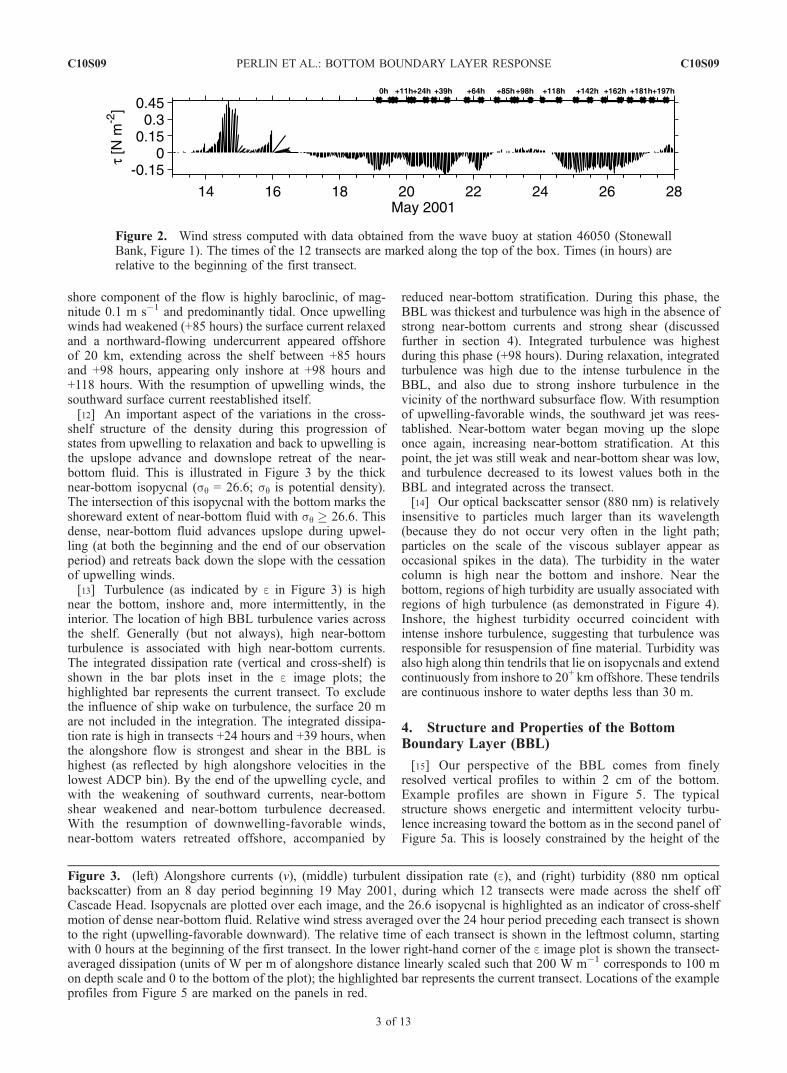
[10] A record of wind stress from the period 6 dayspreceding and during our measurements is shown inFigure 2 (NOAA wave buoy data is used here to showwind stress). Strong, southerly (downwelling-favorable)winds prior to our arrival yielded to northerlies (upwelling-favorable) by the time we began our observations on 19May.Winds remained northerly for 3.5 days, slackening andturning to weak southerly for 2 days before returning againto moderate upwelling-favorable winds for 2.5 days andagain slackening. This timely sequence permitted us theopportunity to obtain detailed observations of the cross-shorestructure of velocity, density, and turbulence through onecomplete and one partial upwelling-relaxation cycle.We haveassigned a time base of hours relative to the beginning of ourobservations to each transect to guide in the description of thetime sequence of events. This is noted at the top of Figure 2.[11] Upwelling-favorable winds had been developing and

building 2 days prior to the beginning of our observations(Figure 2, from the Yaquina Bay wave buoy). By the time ofour first transect (0 hours), a strong southward surfacecurrent extended across the shelf (Figure 3). The surfacecurrent subsequently strengthened and shifted offshore(+24 hours) and back onshore (+64 hours). Superimposedon the wind-driven currents were tidal currents that arespatially and temporally aliased by our sampling scheme.Moored records [Boyd et al., 2002] indicate that the cross-

Figure 1. Bathymetry of the central Oregon coast. Thedark line indicates the location of 12 transects made over theperiod 19–28 May 2001. Locations of the Stonewall Bankwave buoy and mooring are noted.

C10S09 PERLIN ET AL.: BOTTOM BOUNDARY LAYER RESPONSE

2 of 13

C10S09

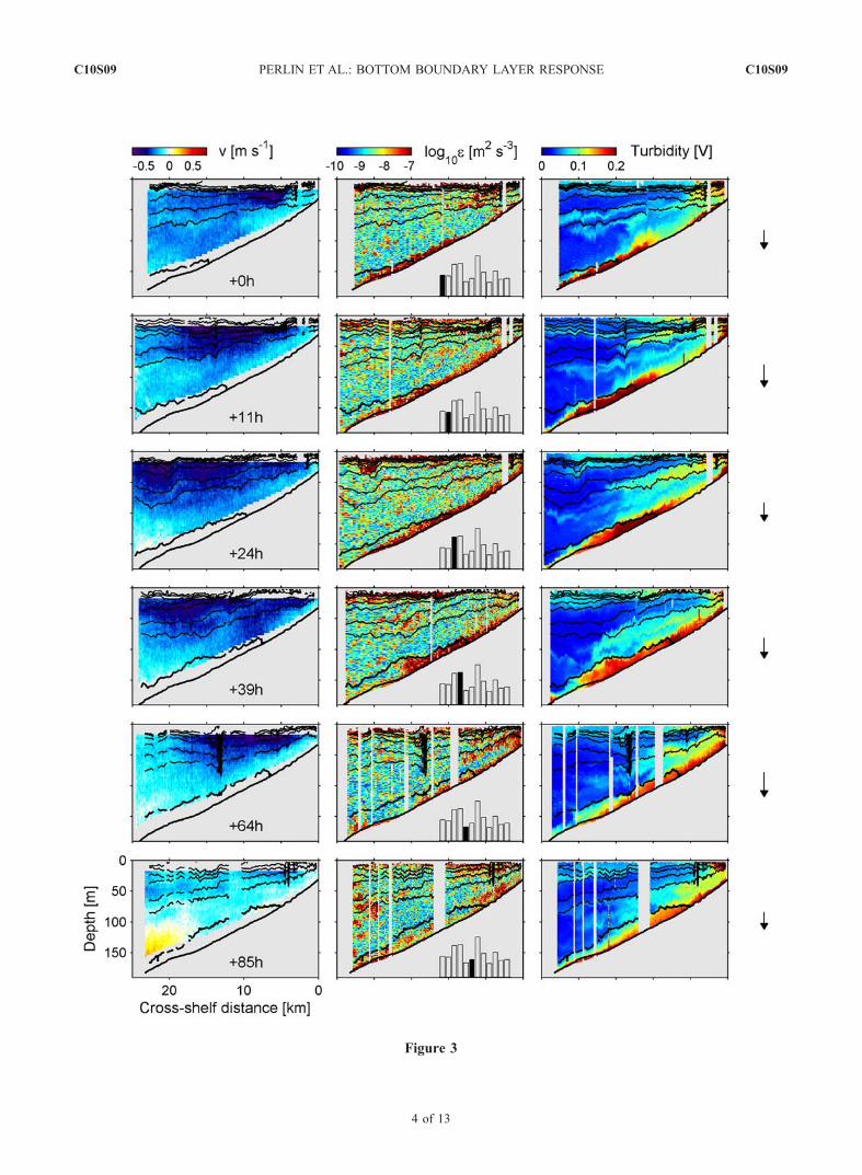
shore component of the flow is highly baroclinic, of mag-nitude 0.1 m s�1 and predominantly tidal. Once upwellingwinds had weakened (+85 hours) the surface current relaxedand a northward-flowing undercurrent appeared offshoreof 20 km, extending across the shelf between +85 hoursand +98 hours, appearing only inshore at +98 hours and+118 hours. With the resumption of upwelling winds, thesouthward surface current reestablished itself.[12] An important aspect of the variations in the cross-

shelf structure of the density during this progression ofstates from upwelling to relaxation and back to upwelling isthe upslope advance and downslope retreat of the near-bottom fluid. This is illustrated in Figure 3 by the thicknear-bottom isopycnal (sq = 26.6; sq is potential density).The intersection of this isopycnal with the bottom marks theshoreward extent of near-bottom fluid with sq � 26.6. Thisdense, near-bottom fluid advances upslope during upwel-ling (at both the beginning and the end of our observationperiod) and retreats back down the slope with the cessationof upwelling winds.[13] Turbulence (as indicated by e in Figure 3) is high

near the bottom, inshore and, more intermittently, in theinterior. The location of high BBL turbulence varies acrossthe shelf. Generally (but not always), high near-bottomturbulence is associated with high near-bottom currents.The integrated dissipation rate (vertical and cross-shelf) isshown in the bar plots inset in the e image plots; thehighlighted bar represents the current transect. To excludethe influence of ship wake on turbulence, the surface 20 mare not included in the integration. The integrated dissipa-tion rate is high in transects +24 hours and +39 hours, whenthe alongshore flow is strongest and shear in the BBL ishighest (as reflected by high alongshore velocities in thelowest ADCP bin). By the end of the upwelling cycle, andwith the weakening of southward currents, near-bottomshear weakened and near-bottom turbulence decreased.With the resumption of downwelling-favorable winds,near-bottom waters retreated offshore, accompanied by

reduced near-bottom stratification. During this phase, theBBL was thickest and turbulence was high in the absence ofstrong near-bottom currents and strong shear (discussedfurther in section 4). Integrated turbulence was highestduring this phase (+98 hours). During relaxation, integratedturbulence was high due to the intense turbulence in theBBL, and also due to strong inshore turbulence in thevicinity of the northward subsurface flow. With resumptionof upwelling-favorable winds, the southward jet was rees-tablished. Near-bottom water began moving up the slopeonce again, increasing near-bottom stratification. At thispoint, the jet was still weak and near-bottom shear was low,and turbulence decreased to its lowest values both in theBBL and integrated across the transect.[14] Our optical backscatter sensor (880 nm) is relatively

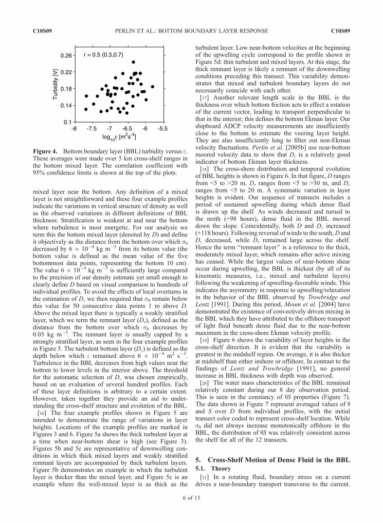
insensitive to particles much larger than its wavelength(because they do not occur very often in the light path;particles on the scale of the viscous sublayer appear asoccasional spikes in the data). The turbidity in the watercolumn is high near the bottom and inshore. Near thebottom, regions of high turbidity are usually associated withregions of high turbulence (as demonstrated in Figure 4).Inshore, the highest turbidity occurred coincident withintense inshore turbulence, suggesting that turbulence wasresponsible for resuspension of fine material. Turbidity wasalso high along thin tendrils that lie on isopycnals and extendcontinuously from inshore to 20+ km offshore. These tendrilsare continuous inshore to water depths less than 30 m.

4. Structure and Properties of the BottomBoundary Layer (BBL)

[15] Our perspective of the BBL comes from finelyresolved vertical profiles to within 2 cm of the bottom.Example profiles are shown in Figure 5. The typicalstructure shows energetic and intermittent velocity turbu-lence increasing toward the bottom as in the second panel ofFigure 5a. This is loosely constrained by the height of the

Figure 2. Wind stress computed with data obtained from the wave buoy at station 46050 (StonewallBank, Figure 1). The times of the 12 transects are marked along the top of the box. Times (in hours) arerelative to the beginning of the first transect.

Figure 3. (left) Alongshore currents (v), (middle) turbulent dissipation rate (e), and (right) turbidity (880 nm opticalbackscatter) from an 8 day period beginning 19 May 2001, during which 12 transects were made across the shelf offCascade Head. Isopycnals are plotted over each image, and the 26.6 isopycnal is highlighted as an indicator of cross-shelfmotion of dense near-bottom fluid. Relative wind stress averaged over the 24 hour period preceding each transect is shownto the right (upwelling-favorable downward). The relative time of each transect is shown in the leftmost column, startingwith 0 hours at the beginning of the first transect. In the lower right-hand corner of the e image plot is shown the transect-averaged dissipation (units of W per m of alongshore distance linearly scaled such that 200 W m�1 corresponds to 100 mon depth scale and 0 to the bottom of the plot); the highlighted bar represents the current transect. Locations of the exampleprofiles from Figure 5 are marked on the panels in red.

C10S09 PERLIN ET AL.: BOTTOM BOUNDARY LAYER RESPONSE

3 of 13

C10S09

Figure 3

C10S09 PERLIN ET AL.: BOTTOM BOUNDARY LAYER RESPONSE

4 of 13

C10S09

Figure 3. (continued)

C10S09 PERLIN ET AL.: BOTTOM BOUNDARY LAYER RESPONSE

5 of 13

C10S09

mixed layer near the bottom. Any definition of a mixedlayer is not straightforward and these four example profilesindicate the variations in vertical structure of density as wellas the observed variations in different definitions of BBLthickness. Stratification is weakest at and near the bottomwhere turbulence is most energetic. For our analysis weterm this the bottom mixed layer (denoted by D) and defineit objectively as the distance from the bottom over which sqdecreased by 6 � 10�4 kg m�3 from its bottom value (thebottom value is defined as the mean value of the fivebottommost data points, representing the bottom 10 cm).The value 6 � 10�4 kg m�3 is sufficiently large comparedto the precision of our density estimate yet small enough toclearly define D based on visual comparison to hundreds ofindividual profiles. To avoid the effects of local overturns inthe estimation of D, we then required that sq remain belowthis value for 50 consecutive data points 1 m above D.Above the mixed layer there is typically a weakly stratifiedlayer, which we term the remnant layer (Dr), defined as thedistance from the bottom over which sq decreases by0.03 kg m�3. The remnant layer is usually capped by astrongly stratified layer, as seen in the four example profilesin Figure 5. The turbulent bottom layer (De) is defined as thedepth below which e remained above 6 � 10�9 m2 s�3.Turbulence in the BBL decreases from high values near thebottom to lower levels in the interior above. The thresholdfor the automatic selection of De was chosen empirically,based on an evaluation of several hundred profiles. Eachof these layer definitions is arbitrary to a certain extent.However, taken together they provide an aid to under-standing the cross-shelf structure and evolution of the BBL.[16] The four example profiles shown in Figure 5 are

intended to demonstrate the range of variations in layerheights. Locations of the example profiles are marked inFigures 3 and 6. Figure 5a shows the thick turbulent layer ata time when near-bottom shear is high (see Figure 3).Figures 5b and 5c are representative of downwelling con-ditions in which thick mixed layers and weakly stratifiedremnant layers are accompanied by thick turbulent layers.Figure 5b demonstrates an example in which the turbulentlayer is thicker than the mixed layer, and Figure 5c is anexample where the well-mixed layer is as thick as the

turbulent layer. Low near-bottom velocities at the beginningof the upwelling cycle correspond to the profile shown inFigure 5d: thin turbulent and mixed layers. At this stage, thethick remnant layer is likely a remnant of the downwellingconditions preceding this transect. This variability demon-strates that mixed and turbulent boundary layers do notnecessarily coincide with each other.[17] Another relevant length scale in the BBL is the

thickness over which bottom friction acts to effect a rotationof the current vector, leading to transport perpendicular tothat in the interior; this defines the bottom Ekman layer. Ourshipboard ADCP velocity measurements are insufficientlyclose to the bottom to estimate the veering layer height.They are also insufficiently long to filter out non-Ekmanvelocity fluctuations. Perlin et al. [2005b] use near-bottommoored velocity data to show that De is a relatively goodindicator of bottom Ekman layer thickness.[18] The cross-shore distribution and temporal evolution

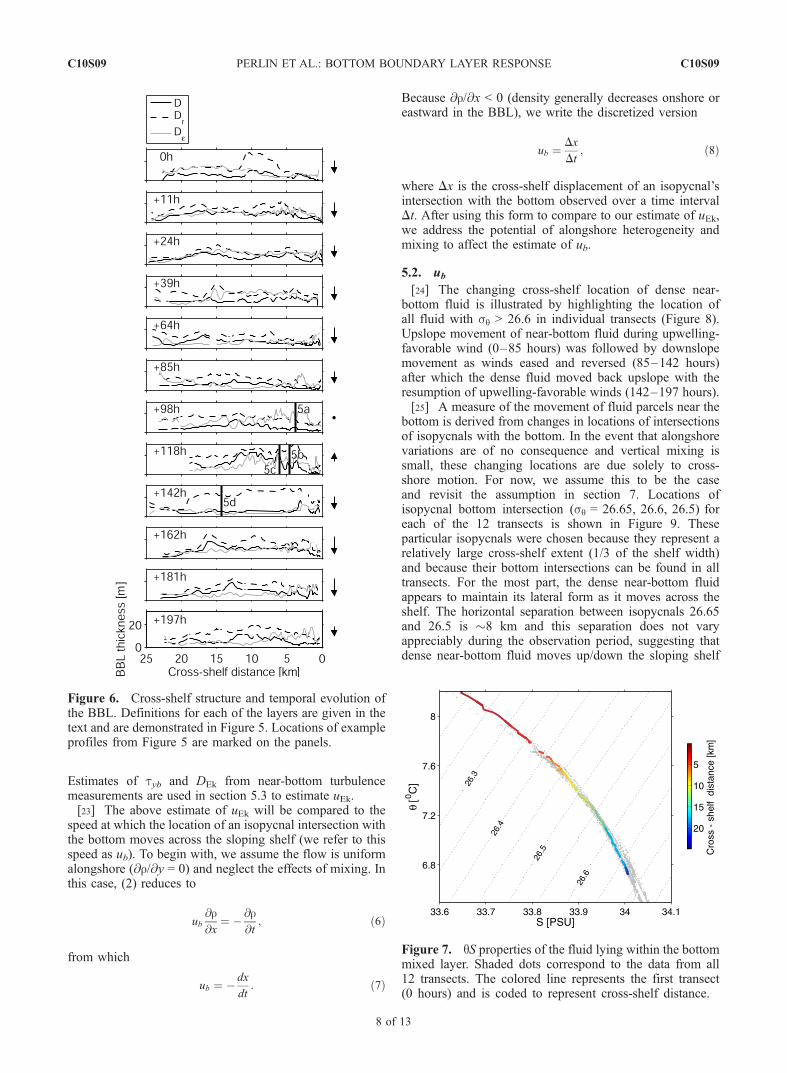
of BBL heights is shown in Figure 6. In that figure, D rangesfrom <5 to >20 m, Dr ranges from <5 to >30 m, and Deranges from <5 to 20 m. A systematic variation in layerheights is evident. Our sequence of transects includes aperiod of sustained upwelling during which dense fluidis drawn up the shelf. As winds decreased and turned tothe north (+98 hours), dense fluid in the BBL moveddown the slope. Coincidentally, both D and De increased(+118 hours). Following reversal of winds to the south,D andDe decreased, while Dr remained large across the shelf.Hence the term ‘‘remnant layer’’ is a reference to the thick,moderately mixed layer, which remains after active mixinghas ceased. While the largest values of near-bottom shearoccur during upwelling, the BBL is thickest (by all of itskinematic measures, i.e., mixed and turbulent layers)following the weakening of upwelling-favorable winds. Thisindicates the asymmetry in response to upwelling/relaxationin the behavior of the BBL observed by Trowbridge andLentz [1991]. During this period, Moum et al. [2004] havedemonstrated the existence of convectively driven mixing inthe BBL which they have attributed to the offshore transportof light fluid beneath dense fluid due to the near-bottommaximum in the cross-shore Ekman velocity profile.[19] Figure 6 shows the variability of layer heights in the

cross-shelf direction. It is evident that the variability isgreatest in the midshelf region. On average, it is also thickerat midshelf than either inshore or offshore. In contrast to thefindings of Lentz and Trowbridge [1991], no generalincrease in BBL thickness with depth was observed.[20] The water mass characteristics of the BBL remained

relatively constant during our 8 day observation period.This is seen in the constancy of qS properties (Figure 7).The data shown in Figure 7 represent averaged values of qand S over D from individual profiles, with the initialtransect color coded to represent cross-shelf location. Whilesq did not always increase monotonically offshore in theBBL, the distribution of qS was relatively consistent acrossthe shelf for all of the 12 transects.

5. Cross-Shelf Motion of Dense Fluid in the BBL

5.1. Theory

[21] In a rotating fluid, boundary stress on a currentdrives a near-boundary transport transverse to the current.

Figure 4. Bottom boundary layer (BBL) turbidity versus e.These averages were made over 5 km cross-shelf ranges inthe bottom mixed layer. The correlation coefficient with95% confidence limits is shown at the top of the plots.

C10S09 PERLIN ET AL.: BOTTOM BOUNDARY LAYER RESPONSE

6 of 13

C10S09

This is the basis of Ekman theory. At an eastern boundary,bottom stress on the southward current formed by thecoastal upwelling circulation drives a bottom Ekman layerup the sloping shelf toward the shore. The dynamics of theboundary layer are described by simplified momentum anddensity equations for a Boussinesq fluid [e.g., Pedlosky,1987]. The alongshore (y coordinate direction) momentumequation reduces to

r0@v

@tþ r0fu ¼ � @p

@yþ @ty

@z: ð1Þ

The density equation reduces to

@r@t

þ u@r@x

þ v@r@y

¼ r0g

@Jb@z

: ð2Þ

Here g is gravitational acceleration; f is the Coriolisparameter; (u, v) is the velocity vector; p is pressure; ty isthe stress component in the y component direction; r isdensity; r0 is background density; and Jb = �(g/r0)r0w0,

which also can be written as Jb = �(g/r0)Kr(@r/@z), wherethe latter represents the definition of the turbulent diffusioncoefficient, Kr, and g is acceleration of gravity.[22] For steady state flow and zero alongshore pressure

gradient, (1) reduces to a classical Ekman balance:

fu ¼ 1

r0

@ty@z

: ð3Þ

Assuming that the shear stress atop the Ekman layer is muchsmaller than the bottom stress, vertical integration of (3) overan Ekman layer of thickness DEk yields the mean cross-shoreEkman transport, JEk, in terms of bottom stress:

JEk ¼tybr0f

: ð4Þ

From this is derived the vertically averaged cross-shoreEkman velocity over DEk:

uEk ¼JEk

DEk

¼ tybr0DEkf

: ð5Þ

Figure 5. Individual Chameleon profiles showing different aspects of the vertical structure of the BBL.Shown here are turbidity sensed by an 880 nm backscatter sensor mounted on Chameleon’s nose,microscale velocity shear, turbulent dissipation rate (e), and sq. The horizontal line in the third panel ofeach plot is an indication of the turbulent boundary layer height (De). In the rightmost column are shownthe heights of mixed layer (D) and remnant layers (Dr) as determined objectively from density profiles. InFigure 5a the turbulent layer is above the remnant layer, in Figure 5b it is in the remnant layer, inFigure 5c it is at the top of the mixed layer (which is approximately collocated with the remnant layer),and in Figure 5d it is contained within a shallow mixed layer.

C10S09 PERLIN ET AL.: BOTTOM BOUNDARY LAYER RESPONSE

7 of 13

C10S09

Estimates of tyb and DEk from near-bottom turbulencemeasurements are used in section 5.3 to estimate uEk.[23] The above estimate of uEk will be compared to the

speed at which the location of an isopycnal intersection withthe bottom moves across the sloping shelf (we refer to thisspeed as ub). To begin with, we assume the flow is uniformalongshore (@r/@y = 0) and neglect the effects of mixing. Inthis case, (2) reduces to

ub@r@x

¼ � @r@t

; ð6Þ

from which

ub ¼ � dx

dt: ð7Þ

Because @r/@x < 0 (density generally decreases onshore oreastward in the BBL), we write the discretized version

ub ¼Dx

Dt; ð8Þ

where Dx is the cross-shelf displacement of an isopycnal’sintersection with the bottom observed over a time intervalDt. After using this form to compare to our estimate of uEk,we address the potential of alongshore heterogeneity andmixing to affect the estimate of ub.

5.2. ub[24] The changing cross-shelf location of dense near-

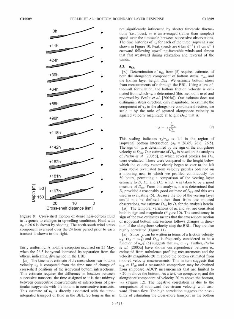
bottom fluid is illustrated by highlighting the location ofall fluid with sq > 26.6 in individual transects (Figure 8).Upslope movement of near-bottom fluid during upwelling-favorable wind (0–85 hours) was followed by downslopemovement as winds eased and reversed (85–142 hours)after which the dense fluid moved back upslope with theresumption of upwelling-favorable winds (142–197 hours).[25] A measure of the movement of fluid parcels near the

bottom is derived from changes in locations of intersectionsof isopycnals with the bottom. In the event that alongshorevariations are of no consequence and vertical mixing issmall, these changing locations are due solely to cross-shore motion. For now, we assume this to be the caseand revisit the assumption in section 7. Locations ofisopycnal bottom intersection (sq = 26.65, 26.6, 26.5) foreach of the 12 transects is shown in Figure 9. Theseparticular isopycnals were chosen because they represent arelatively large cross-shelf extent (1/3 of the shelf width)and because their bottom intersections can be found in alltransects. For the most part, the dense near-bottom fluidappears to maintain its lateral form as it moves across theshelf. The horizontal separation between isopycnals 26.65and 26.5 is 8 km and this separation does not varyappreciably during the observation period, suggesting thatdense near-bottom fluid moves up/down the sloping shelf

Figure 6. Cross-shelf structure and temporal evolution ofthe BBL. Definitions for each of the layers are given in thetext and are demonstrated in Figure 5. Locations of exampleprofiles from Figure 5 are marked on the panels.

Figure 7. qS properties of the fluid lying within the bottommixed layer. Shaded dots correspond to the data from all12 transects. The colored line represents the first transect(0 hours) and is coded to represent cross-shelf distance.

C10S09 PERLIN ET AL.: BOTTOM BOUNDARY LAYER RESPONSE

8 of 13

C10S09

fairly uniformly. A notable exception occurred on 25 May,when the 26.5 isopycnal increased its separation from theothers, indicating divergence in the BBL.[26] The kinematic estimate of the cross-shore near-bottom

velocity ub is computed from the time rate of change ofcross-shelf positions of the isopycnal bottom intersections.This estimate requires the difference in location betweensuccessive transects; the time assigned to it is that midwaybetween consecutive measurements of intersections of par-ticular isopycnals with the bottom in consecutive transects.This estimate of ub is directly associated with the time-integrated transport of fluid in the BBL. So long as this is

not significantly influenced by shorter timescale fluctua-tions (i.e., tides), ub is an averaged (rather than sampled)speed over the timescale between successive observations.The time histories of ub for each of the three isopycnals areshown in Figure 10. Peak speeds are 6 km d�1 (7 cm s�1)eastward following upwelling-favorable winds and almostthat fast westward during relaxation and reversal of thewinds.

5.3. uEk[27] Determination of uEk from (5) requires estimates of

both the alongshore component of bottom stress, tyb, andthe Ekman layer height, DEk. We estimate bottom stressfrom measurements of e through the BBL. Using a law-of-the-wall formulation, the bottom friction velocity is esti-mated from which tb is determined (this method is used andreviewed by Perlin et al. [2005a]). Our estimate does notdistinguish stress direction, only magnitude. To estimate thecomponent of tb in the alongshore coordinate direction, wescale it by the ratio of squared alongshore velocity tosquared velocity magnitude at height DEk; that is,

tyb ¼ tbv2DEk

U 2DEk

: ð9Þ

This scaling indicates tb/tyb 1.1 in the region ofisopycnal bottom intersection (sq = 26.65, 26.6, 26.5).The sign of tyb is determined by the sign of the alongshorevelocity at DEk. Our estimate of DEk is based on the analysisof Perlin et al. [2005b], in which several proxies for DEk

were evaluated. These were compared to the height belowwhich the velocity vector clearly began to veer to the leftfrom above (evaluated from velocity profiles obtained ona mooring near to which we profiled continuously for50 hours, permitting a comparison of the veering layerestimate to D, Dr, and De), which was taken to be a goodmeasure of DEk. From this analysis, it was determined thatDe provided a reasonably good estimate of DEk and this wasused in evaluating (5). Because the top of the veering layercould not be defined other than from the mooredobservations, we estimate DEk by De for the analysis herein.[28] The temporal variations of ub and uEk are consistent

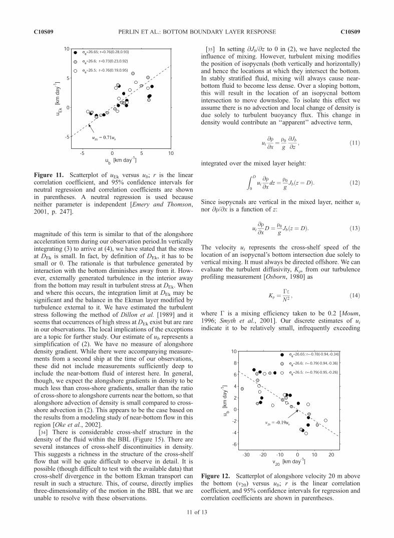
both in sign and magnitude (Figure 10). The consistency insign of the two estimates means that the cross-shore motionof isopycnal bottom intersections follows changes in direc-tion of the alongshore velocity atop the BBL. They are alsohighly correlated (Figure 11).[29] Since tb can be written in terms of a friction velocity

u*, (tb = ru

*2) and DEk is frequently considered to be a

function of u*/f, (5) suggests that uEk / u

*. Further, Perlin

et al. [2005a] have shown correspondence between u*

estimated from turbulence profiling measurements and thevelocity magnitude 20 m above the bottom estimated frommoored velocity measurements. This in turn suggests thatuEk / U20 and a reasonable comparison may be obtainedfrom shipboard ADCP measurements that are limited to20 m above the bottom. As a test, we compare ub and thealongshore component of velocity 20 m above the bottom,v20 (Figure 12). The negative correlation is due to thecomparison of southward free-stream velocity with east-ward Ekman flow. The high correlation suggests the possi-bility of estimating the cross-shore transport in the bottom

Figure 8. Cross-shelf motion of dense near-bottom fluidin response to changes in upwelling conditions. Fluid withsq > 26.6 is shown by shading. The north-south wind stresscomponent averaged over the 24 hour period prior to eachtransect is shown to the right.

C10S09 PERLIN ET AL.: BOTTOM BOUNDARY LAYER RESPONSE

9 of 13

C10S09

Ekman layer from shipboard ADCP measurements ormoored measurements well above the bottom.

6. Bottom Ekman Balance Over a 3 MonthMoored Record

[30] An extended test of the Ekman balance (4) in theBBL using moored data requires an indirect estimate of tb.The result from Perlin et al. [2005a], u*

2 = CD20U20

2 , isexpressed in terms of a drag coefficient evaluated at 20 mheight, CD

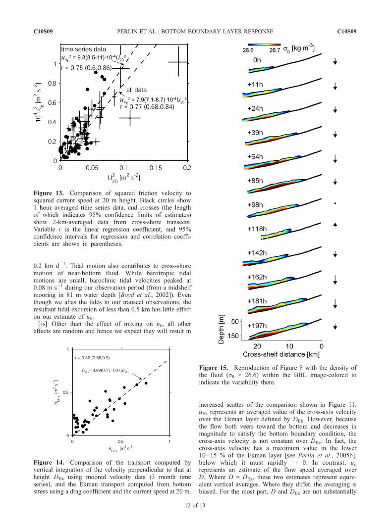
20 = 9.8 � 10�4. For comparison, a similarcorrespondence is evaluated using the observations dis-cussed in this paper. In this case, U20 represents the currentspeed from shipboard ADCP averaged over 2 km as wetransited across the shelf (u

*is averaged similarly from the

turbulence profiles made over the same span of the shelf).The addition of the transect observations to the stationaryobservations results in CD

20 = 7.9 � 10�4 (Figure 13). (Thelarger scatter and smaller value of CD

20 from the transectobservations may be a consequence of spatial variations inthe velocity measured from shipboard ADCP compared toan ADCP measure of velocity at a fixed position.)[31] The moored velocity observations used to define CD

20

by Perlin et al. [2005a] from our 50 hour turbulenceprofiling time series extended for a period of 3 monthsfrom 15 May to 28 August 2001 [Boyd et al., 2002]. UsingCD20, we compute the Ekman transport in the bottom

boundary layer as JEk t = CD20U20

2 /f, where tb has beenreplaced by rCD

20U202 . We compare this to

JEk v ¼ZDv

0

u?dz; ð10Þ

where u?(z) is the observed velocity perpendicular to that atheight Dv, from a daily-averaged velocity profile filtered toremove currents at tidal periods and shorter. Because De isnot available from our moored observations, as it is fromour profiling observations, Dv is used for this particularanalysis. Dv was defined by Perlin et al. [2005b] to be the

height at which the veering of the detided velocity towardthe bottom begins. For the comparison, we have used thevalue of CD

20 = 9.8 � 10�4, determined from coincident andcollocated velocity and turbulence measurements. Theresult (Figure 14) indicates a bottom boundary layer inrelative agreement with an Ekman balance over the 3 monthduration of the mooring deployment. (For this analysis, twocriteria were applied to the daily-averaged velocity profiles:(1) velocity at 8 m height �0.05 m s�1 and (2) direction wasrequired to be steady over 2 consecutive days.)

7. Discussion

[32] Aside from the contributions of uncertainties in ourestimates of tb and DEk to the uncertainty in uEk, there aretwo terms in the alongshore momentum equation defined by(1) that we have neglected, each of which contribute to theuncertainty in our estimate of uEk. First, we have neglectedlocal acceleration of the alongshore flow. This term can beestimated from the rate of change of mean alongshorecurrent between consecutive transects. Our analysis indi-cates that 1/f(dv/dt) is typically 10–30% of the magnitudeof uEk. When added to uEk in comparison to ub, thecorrelation is marginally improved.[33] Secondly, we have no measure of the alongshore

pressure gradient @p/@y. However, results from a regionalmodel described by Kurapov et al. [2005] suggest that the

Figure 9. Cross-shore location of the intersectionwhere three isopycnals interesct the bottom for all of the12 transects. At the top of the plot are wind stress vectors.

Figure 10. Cross-shelf speed of dense near-bottom fluiddetermined from the rate of change of the intersection ofisopycnals corresponding to sq = 26.5, 26.6, and 26.65 withthe bottom (ub) and the mean Ekman velocity estimatedfrom bottom stress (uEk). Speeds are >0 on-shelf.

C10S09 PERLIN ET AL.: BOTTOM BOUNDARY LAYER RESPONSE

10 of 13

C10S09

magnitude of this term is similar to that of the alongshoreacceleration term during our observation period.In verticallyintegrating (3) to arrive at (4), we have stated that the stressat DEk is small. In fact, by definition of DEk, it has to besmall or 0. The rationale is that turbulence generated byinteraction with the bottom diminishes away from it. How-ever, externally generated turbulence in the interior awayfrom the bottom may result in turbulent stress at DEk. Whenand where this occurs, the integration limit at DEk may besignificant and the balance in the Ekman layer modified byturbulence external to it. We have estimated the turbulentstress following the method of Dillon et al. [1989] and itseems that occurrences of high stress at DEk exist but are rarein our observations. The local implications of the exceptionsare a topic for further study. Our estimate of ub represents asimplification of (2). We have no measure of alongshoredensity gradient. While there were accompanying measure-ments from a second ship at the time of our observations,these did not include measurements sufficiently deep toinclude the near-bottom fluid of interest here. In general,though, we expect the alongshore gradients in density to bemuch less than cross-shore gradients, smaller than the ratioof cross-shore to alongshore currents near the bottom, so thatalongshore advection of density is small compared to cross-shore advection in (2). This appears to be the case based onthe results from a modeling study of near-bottom flow in thisregion [Oke et al., 2002].[34] There is considerable cross-shelf structure in the

density of the fluid within the BBL (Figure 15). There areseveral instances of cross-shelf discontinuities in density.This suggests a richness in the structure of the cross-shelfflow that will be quite difficult to observe in detail. It ispossible (though difficult to test with the available data) thatcross-shelf divergence in the bottom Ekman transport canresult in such a structure. This, of course, directly impliesthree-dimensionality of the motion in the BBL that we areunable to resolve with these observations.

[35] In setting @Jb/@z to 0 in (2), we have neglected theinfluence of mixing. However, turbulent mixing modifiesthe position of isopycnals (both vertically and horizontally)and hence the locations at which they intersect the bottom.In stably stratified fluid, mixing will always cause near-bottom fluid to become less dense. Over a sloping bottom,this will result in the location of an isopycnal bottomintersection to move downslope. To isolate this effect weassume there is no advection and local change of density isdue solely to turbulent buoyancy flux. This change indensity would contribute an ‘‘apparent’’ advective term,

ui@r@x

¼ r0g

@Jb@z

; ð11Þ

integrated over the mixed layer height:

Z D

0

ui@r@x

dz ¼ r0gJb z ¼ Dð Þ: ð12Þ

Since isopycnals are vertical in the mixed layer, neither uinor @r/@x is a function of z:

ui@r@x

D ¼ r0gJb z ¼ Dð Þ: ð13Þ

The velocity ui represents the cross-shelf speed of thelocation of an isopycnal’s bottom intersection due solely tovertical mixing. It must always be directed offshore. We canevaluate the turbulent diffusivity, Kr, from our turbulenceprofiling measurement [Osborn, 1980] as

Kr ¼GeN2

; ð14Þ

where G is a mixing efficiency taken to be 0.2 [Moum,1996; Smyth et al., 2001]. Our discrete estimates of uiindicate it to be relatively small, infrequently exceeding

Figure 11. Scatterplot of uEk versus ub; r is the linearcorrelation coefficient, and 95% confidence intervals forneutral regression and correlation coefficients are shownin parentheses. A neutral regression is used becauseneither parameter is independent [Emery and Thomson,2001, p. 247].

Figure 12. Scatterplot of alongshore velocity 20 m abovethe bottom (v20) versus ub; r is the linear correlationcoefficient, and 95% confidence intervals for regression andcorrelation coefficients are shown in parentheses.

C10S09 PERLIN ET AL.: BOTTOM BOUNDARY LAYER RESPONSE

11 of 13

C10S09

0.2 km d�1. Tidal motion also contributes to cross-shoremotion of near-bottom fluid. While barotropic tidalmotions are small, baroclinic tidal velocities peaked at0.08 m s�1 during our observation period (from a midshelfmooring in 81 m water depth [Boyd et al., 2002]). Eventhough we alias the tides in our transect observations, theresultant tidal excursion of less than 0.5 km has little effecton our estimate of ub.[36] Other than the effect of mixing on ub, all other

effects are random and hence we expect they will result in

increased scatter of the comparison shown in Figure 11.uEk represents an averaged value of the cross-axis velocityover the Ekman layer defined by DEk. However, becausethe flow both veers toward the bottom and decreases inmagnitude to satisfy the bottom boundary condition, thecross-axis velocity is not constant over DEk. In fact, thecross-axis velocity has a maximum value in the lower10–15 % of the Ekman layer [see Perlin et al., 2005b],below which it must rapidly ! 0. In contrast, ubrepresents an estimate of the flow speed averaged overD. Where D = DEk, these two estimates represent equiv-alent vertical averages. Where they differ, the averaging isbiased. For the most part, D and DEk are not substantially

Figure 13. Comparison of squared friction velocity tosquared current speed at 20 m height. Black circles show1 hour averaged time series data, and crosses (the lengthof which indicates 95% confidence limits of estimates)show 2-km-averaged data from cross-shore transects.Variable r is the linear regression coefficient, and 95%confidence intervals for regression and correlation coeffi-cients are shown in parentheses.

Figure 14. Comparison of the transport computed byvertical integration of the velocity perpendicular to that atheight DEk using moored velocity data (3 month timeseries), and the Ekman transport computed from bottomstress using a drag coefficient and the current speed at 20 m.

Figure 15. Reproduction of Figure 8 with the density ofthe fluid (sq > 26.6) within the BBL image-colored toindicate the variability there.

C10S09 PERLIN ET AL.: BOTTOM BOUNDARY LAYER RESPONSE

12 of 13

C10S09

different (Figure 6) and this effect is not likely to besignificant.

8. Summary

[37] By repeating transects of currents, density, andturbulence through the BBL across a relatively uniformstretch of the continental shelf off Oregon, we have beenable to observe the response of the BBL to variations inwinds and currents in some detail. We had the good fortuneto make these observations coincident with a sequence ofstrong upwelling-favorable winds followed by relaxationand subsequent resumption of upwelling.[38] By all measures, the thickness of the BBL is greatest

and turbulence there is most intense during the relaxationfrom upwelling. This is consistent with the observations ofTrowbridge and Lentz [1991]. From a subset of the obser-vations described here, Moum et al. [2004] have suggestedhow convectively driven mixing can be responsible forboth the intense mixing and thickened boundary layer aslight near-bottom fluid is drawn beneath denser fluidduring downslope flow. Upon the resumption of upwelling-favorable winds, and when the downslope motion ceases,turbulence dies in the absence of other sources (low currentvelocities in the interior and therefore low levels of shear-generated turbulence near the bottom). The well-mixedbottom layer thins, leaving a thick remnant layer withlow stratification. Advection of dense near-bottom fluidupslope by Ekman transport during upwelling increases thedensity difference between the boundary layer and theinterior, so that vertical transport near the top of the layeris suppressed, and the growth of the BBL is inhibited.[39] By tracking the intersection of near-bottom isopycnals

with the bottom over successive transects, we estimate thecross-shore speed of near-bottom fluid ub. This estimate isbased on the transport of fluid with specific density. Itcorrelates well and is approximately equal to a dynamicestimate of mean Ekman velocity. This test suggests thatthe Ekman balance holds across a significant cross-shoreextent of the continental shelf, not only at a particular location[Trowbridge and Lentz, 1998]. By extending this calcula-tion to a 3 month record of moored velocities, we verifythe Ekman balance in the BBL over the period 15 May to28 August 2001, at a midshelf location on the Oregon coast.

[40] Acknowledgments. This work was funded by the NationalScience Foundation. Mike Neeley-Brown, Ray Kreth, Greig Thompson,and Gunnar Gunderson helped to obtain these data. The moored velocitydata was kindly provided by Tim Boyd, Mike Kosro, and Murray Levine.The captain and crew of the R/V T. G. Thompson were helpful in allregards.

ReferencesBoyd, T., M. D. Levine, P. M. Kosro, S. R. Gard, and W. Waldorf (2002),Observations from moorings on the Oregon continental shelf, May–August 2001, Data Rep. 190 2002-6, Oregon State Univ., Corvallis.

Dickey, T. D., and J. C. van Leer (1984), Observations and simulationsof bottom Ekman layer on a continental shelf, J. Geophys. Res., 89,1983–1988.

Dillon, T. M., J. N. Moum, T. K. Chereskin, and D. R. Caldwell (1989),Zonal momentum balance at the equator, J. Phys. Oceanogr., 19,561–570.

Emery, W. J., and R. E. Thomson (2001), Data Analysis Methods inPhysical Oceanography, 2nd ed., 638 pp., Elsevier, New York.

Kundu, P. K. (1976), Ekman veering observed near the ocean bottom,J. Phys. Oceanogr., 6, 238–242.

Kurapov, A. L., J. S. Allen, G. Egbert, R. Miller, P. M. Kosro, M. D.Levine, T. Boyd, J. A. Barth, and J. N. Moum (2005), Assimilation ofmoored velocity data in a model of coastal wind-driven circulation offOregon: Multivariate capabilities, J. Geophys. Res., doi:10.1029/2004JC002493, in press.

Lass, H. U., and V. Mohrholz (2003), On dynamics and mixing of inflow-ing saltwater in the Arkona Sea, J. Geophys. Res., 108(C2), 3042,doi:10.1029/2002JC001465.

Lentz, S. J., and J. H. Trowbridge (1991), The bottom boundarylayer over the northern California shelf, J. Phys. Oceanogr., 21,1186–1201.

Mercado, A., and J. van Leer (1976), Near bottom velocity and temperatureprofiles observed by cyclosonde, Geophys. Res. Lett., 3, 633–636.

Moum, J. N. (1996), Efficiency of mixing in the main thermocline,J. Geophys. Res., 101, 12,057–12,069.

Moum, J. N., M. C. Gregg, R. C. Lien, and M. E. Carr (1995),Comparison of turbulence kinetic energy dissipation rate estimatesfrom two ocean microstructure profilers, J. Atmos. Oceanic Technol.,12, 346–366.

Moum, J. N., A. Perlin, J. M. Klymak, M. D. Levine, T. Boyd, and P. M.Kosro (2004), Convectively-driven mixing in the bottom boundary layerover the continental shelf during downwelling, J. Phys. Oceanogr., 34,2189–2202.

Oke, P. R., J. S. Allen, R. N. Miller, and G. D. Egbert (2002), Amodeling study of the three-dimensional continental shelf circulationoff Oregon. Part II: Dynamical analysis, J. Phys. Oceanogr., 32,1383–1403.

Osborn, T. R. (1980), Estimates of the local rate of vertical diffusion fromdissipation measurements, J. Phys. Oceanogr., 10, 83–89.

Pedlosky, J. (1987), Geophysical Fluid Dynamics, 2nd ed., 710 pp.,Springer, New York.

Perlin, A., J. N. Moum, J. M. Klymak, M. D. Levine, T. Boyd, and P. M.Kosro (2005a), A modified law-of-the-wall applied to oceanic bottomboundary layers, J. Geophys. Res., doi:10.1029/2004JC002310, inpress.

Perlin, A., J. N. Moum, J. M. Klymak, M. D. Levine, T. Boyd, and P. M.Kosro (2005b), Concentration of Ekman transport in the bottom bound-ary layer by stratification, J. Geophys. Res., doi:10.1029/2004JC002641,in press.

Saylor, J. H. (1994), Studies of bottom Ekman layer processes and mid-lakeupwelling in the Laurentian Great Lakes, Water Pollut. Res. J. Can., 29,233–246.

Saylor, J. H., and G. M. Miller (1988), Observation of Ekman veering at thebottom of Lake Michigan, J. Great Lakes Res., 14, 94–100.

Smyth, W. D., J. N. Moum, and D. R. Caldwell (2001), The efficiency ofmixing in turbulent patches: Inferences from direct simulations andmicrostructure observations, J. Phys. Oceanogr., 31, 1969–1992.

Trowbridge, J. H., and S. J. Lentz (1991), Asymmetric behavior of anoceanic boundary layer above a sloping bottom, J. Phys. Oceanogr.,21, 1171–1185.

Trowbridge, J. H., and S. J. Lentz (1998), Dynamics of the bottomboundary layer on the northern California shelf, J. Phys. Oceanogr.,28, 2075–2093.

Weatherly, G. L. (1972), A study of the bottom boundary layer of theFlorida current, J. Phys. Oceanogr., 2, 54–72.

�����������������������J. M. Klymak, Scripps Institution of Oceanography, University of

California, San Diego, 9500 Gilman Drive, La Jolla, CA 92093-0213, USA.( jklymak@ucsd.edu)J. N. Moum and A. Perlin, College of Oceanic and Atmospheric

Sciences, 104 Ocean Admin Building, Oregon State University, Corvallis,OR 97331-5503, USA. (moum@coas.oregonstate.edu; aperlin@coas.oregonstate.edu)

C10S09 PERLIN ET AL.: BOTTOM BOUNDARY LAYER RESPONSE

13 of 13

C10S09