Response time analysis with offset Master Thesis in Information and Communication Technology NGUYEN HONG VUONG Department of Information & Communication Technology UNIVERSITY OF SCIENCE AND TECHNOLOGY OF HANOI Intake 2011-2013 Supervisor: Professor Frank Singhoff UNIVERSITY OF BREST Tutor: Associated Professor Daniel Chillet UNIVERSITY OF RENNES 1, ENSSAT
Transcript
Response time analysis with offsetMaster Thesis in Information and Communication Technology
NGUYEN HONG VUONG
Department of Information & Communication TechnologyUNIVERSITY OF SCIENCE AND TECHNOLOGY OF HANOI
Intake 2011-2013
Supervisor: Professor Frank SinghoffUNIVERSITY OF BREST
Tutor: Associated Professor Daniel ChilletUNIVERSITY OF RENNES 1, ENSSAT
Contents
1 Introduction 2
2 Related works 32.1 Response time analysis with offset . . . . . . . . . . . . . . . . . . . . . . . . . . . 32.2 Response time analysis for CAN network . . . . . . . . . . . . . . . . . . . . . . . 3
1 A task set that is unschedulable without offset . . . . . . . . . . . . . . . . . . . . . 182 A poorly designed system leads to pessimistic response time . . . . . . . . . . . . 193 Task transformation makes response time of tasks more optimistic . . . . . . . . . 20
ii
Abstract
Cheddar is a toolset based on real-time scheduling and queueing system theory, and is usedto verify timing constraints of real-time systems. Currently the Cheddar team is looking for moredistributed system support implemented into Cheddar.
CAN network has been used in automotive, and at least one generation of car is using offsetfor scheduling. However, no analysis tool was used, thus left the utilization of CAN network ata very low level. Because of that, the Cheddar team also want to implement offset support intoCheddar.
This work involves investigating, evaluating and implementing response time analysis algo-rithms with offset into the Cheddar toolset.
1
1 Introduction
The context of this research is the SMART project, which is a collaborative project between Lab-STICC UBO, Ellidis Technologies and Virtualys. Lab-STICC UBO, in the framework of SMARTproject, is developing the Cheddar toolset.
The Cheddar toolset is based on real-time scheduling and queueing system theory. The Cheddartoolset was developed to provide a tool for verifying timing constraints of real-time systems. Thecurrent implementation of Cheddar has very limited support for distributed system.
At the same time, in the framework of the SMART project, we need to model and verify a real-timesystem based on CAN network. The system is used in an automotive project.
Given the situation, we aim to investigate, evaluate and implement into Cheddar response timeanalysis algorithms that support CAN network in particular and distributed systems in general.The chosen technique is response time analysis (RTA) with offset.
The layout of this report: Section 2 gives background information on this work and works ofother authors that relate to scheduling theory and CAN network. Section 3 shows the reason forchoosing offset for this work. Section 4 gives the analysis on chosen algorithms. Section 5 givesthe methodology for evaluation and the result of implemented algorithms. Finally, Section 6 giveshindsights and possible extensions to this work.
2
2 Related works
This work aim to investigate, evaluate and implement RTA algorithms with offset into Cheddar.This section gives brief view of the research background, many of which can be the target toextend this work.
2.1 Response time analysis with offset
The first foundation for RTA with offset was laid by Audsley et al.: both RM and DM priority assign-ment algorithms are not optimal for system with offset or abitrary deadline. Due to this, Audsleyet al. developed an optimal priority assignment algorithm called ”Bottom up” [2].
Offset assignment is another pre-analysis problem alongside with priority assignment. In systemswhere offset are set by the scheduling algorithm (offset free systems), Grenier et al. developedseveral algorithms to assign offset and priority together - since offset free can make priority as-signment non-optimal: the optimal method, dissimilar method or heuristics method [15].
Analysis algorithms for fixed priority systems with fixed offset were developed by Audsley et al.and Tindell [6] [7]. Later on, Palencia et al. developed a technique that allow dynamic and abitraryoffset on fixed priority systems; after that Palencia et al. extended the technique to also supportdynamic priority systems [9] [11].
Implementation-wise, Maki-Turja et al. developed a technique to optimize the implementation ofTindell [7] and Palencia [9] algorithms for faster computation time. The increasement in perfor-mance was shown in benchmarks [12].
2.2 Response time analysis for CAN network
The foundation was laid by Tindell et al.: they first proposed a method to calculate worst-case re-sponse time of CAN messages by mapping CAN specified concepts and traditional RTA concepts[4]. Later, Dobrin et al. presented a method that transform RTA non-compatible offline scheduledtransmission schemes into RTA compatible sets of messages [13]. Choquet-Geniet et al. on theother hand showed that systems with offset will also produce a cyclic schedule, thus is compatiblewith off-line scheduling [14].
Alongside with traditional priority-based RTA, CAN network nodes can also operate with a FIFOqueue. There have been researches on RTA on CAN network that have some node are priority-based, where others are FIFO queue-based [17].
Very recently, the benefit of using offset to reduce WCRT has been proven using benchmarks byGrenier et al. and Yomsi et al. [16] [18].
3
3 Motivation
In this section, we will provide information on why Offset were chosen as the solution, and whatthe Cheddar team were looking for to implement into Cheddar.
3.1 Timing models
In an system using offset, related tasks are grouped into transactions that can arrive periodicallyor sporadically - thus transactions have an attribute called period, depicted as the minimal timebetween two successive arrival of the transaction.
Offset is defined as the time between the arrival of the transaction and the actual release of thetask [6] [7].
Ai
Oi
T
Bi + J
i + C
i
nth arrivaln+1th arrival
Figure 1: Timing model.
A CAN frame is modelled as a task with the following attributes [3] [18] (Fig. 1):
• Period T: frames are sent by application tasks running in CAN nodes. Thus, frames inheritthe ”period” attribute of such tasks.
• Jitter J: release jitter is another characteristic of application tasks that frames inherit from.
• Capacity C: the time needed to transmit a frame end-to-end. It is deliverable from the sizeof the frames (including CAN-specified additional data) and the network bandwidth.
• Deadline D: a relative deadline for a frame to be transmited.
• Blocking time B.
• Worst-case response time R: the longest time taken to deliver a frame end-to-end.
3.2 Motivation of using offset
The classic response time analysis techinques (RMA, DMA) assume that the tasks are indepen-dent. In fact, the dependencies between tasks can still be expressed via their priorities. Dependson the technique used, the priority of each task can be easily changed by changing the appropri-ate attribute of the task. However, this can greatly affect the design of the system being scheduleditself.
Example 3.2.1:
4
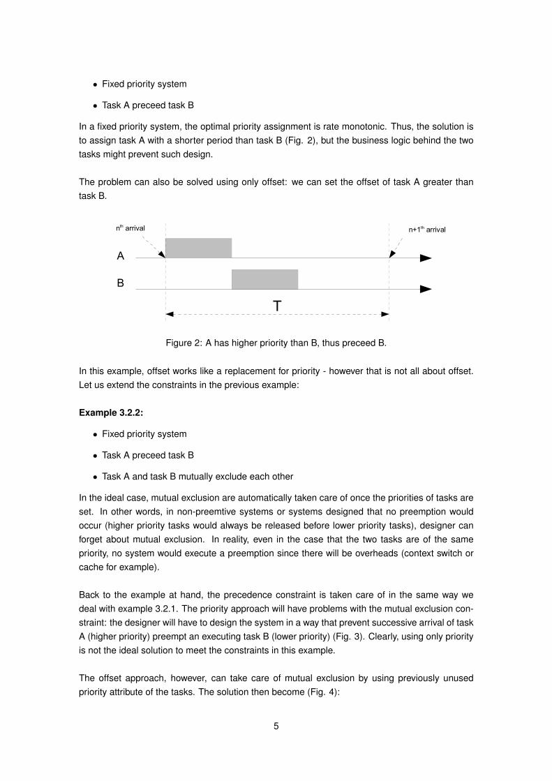
• Fixed priority system
• Task A preceed task B
In a fixed priority system, the optimal priority assignment is rate monotonic. Thus, the solution isto assign task A with a shorter period than task B (Fig. 2), but the business logic behind the twotasks might prevent such design.
The problem can also be solved using only offset: we can set the offset of task A greater thantask B.
T
nth arrival n+1th arrival
A
B
Figure 2: A has higher priority than B, thus preceed B.
In this example, offset works like a replacement for priority - however that is not all about offset.Let us extend the constraints in the previous example:
Example 3.2.2:
• Fixed priority system
• Task A preceed task B
• Task A and task B mutually exclude each other
In the ideal case, mutual exclusion are automatically taken care of once the priorities of tasks areset. In other words, in non-preemtive systems or systems designed that no preemption wouldoccur (higher priority tasks would always be released before lower priority tasks), designer canforget about mutual exclusion. In reality, even in the case that the two tasks are of the samepriority, no system would execute a preemption since there will be overheads (context switch orcache for example).
Back to the example at hand, the precedence constraint is taken care of in the same way wedeal with example 3.2.1. The priority approach will have problems with the mutual exclusion con-straint: the designer will have to design the system in a way that prevent successive arrival of taskA (higher priority) preempt an executing task B (lower priority) (Fig. 3). Clearly, using only priorityis not the ideal solution to meet the constraints in this example.
The offset approach, however, can take care of mutual exclusion by using previously unusedpriority attribute of the tasks. The solution then become (Fig. 4):
5
A1
T
nth arrival n+1th arrival
A
B
A2
preemption
Figure 3: A has higher priority than B, thus preempt B.
• Give A a smaller offset than B so that A preceed B.
• Give B an offset so that even in the case that A experiences WCRT, A still finishs before Bis released. (OB ≥ OA + RA)
• Give B higher priority than A so that A can never preempt B.
A1
T
nth arrival n+1th arrival
A
B
A2
OB
OA1
OA2
Figure 4: A has lower priority than B, thus cannot preempt B.
In reality, there can be a mandatory delay between the finish of task A and the begin of task B.Such delay can be introduced due to various reasons: task A and B might be exchanging mes-sages, and there must be a certain amount of time to deliver the message. Another common usecase is the I/O time: since the task cannot suspend itself, the designer can make a decision ofbreaking the task into two. Often enough the reason is the I/O time, which can be large than theexecution of the task itself. The idea is to release the CPU during I/O, since the CPU will be freeanyway. Thus the example can be extended as follow:
Example 3.2.3
• Fixed priority system
• Task A preceed task B
• Task A and task B mutually exclude each other
• There must be a minimum of ∆ time units after A is finished and before B is released
6
With priority alone, such timing pattern between A and B is unachievable. The offset approach(Fig. 5), however, is sufficient with a minimal change to the solution from example 3.1.2:
OB ≥ OA + RA + ∆AB
T
nth arrival n+1th arrival
A
BO
B
OA
∆AB
Figure 5: Using offset to express mandatory delay between two tasks.
In addition to task dependencies, offset can also be used to support systems with asynchronouscommunication between tasks.
Communication between task on a same system can be achieved using the producer-consumermodel. Such design would require a priority ceiling protocol to control accesses to shared re-source - unless there are no concurent accesses to the shared resource. Such condition caneasily be achieved using offset: let us say that task A and task B access to the same sharedresource. We can assign task B an offset that is greater than the worst case response time oftask A plus task A offset. This way task A and task B will never be executed in parallel, thus theuse of a PCP is not needed. This is actually the same solution as of example 3.2.2 (Fig. 4).
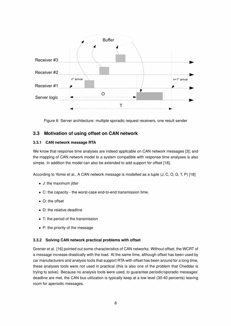
Tindell [8] mentioned an use case for offset in interprocessor communication. The system use aclient-server model: client tasks send messages to a server task, awaiting for the reply. Servertasks wait for a message arrival and activate itself, execute the business logic and return the resultto the client task.
To implement such architecture, a solution is to transform client tasks by breaking each of theminto two child tasks: one that sends, and one that receives. The dependencies between such twotask is exactly the same as in example 3.2.3 (Fig. 5); in other words offset can be used.
The previous design has a flaw however: each server task can only receive one message - inother words, one server task for each message sent. This introduce response time and resourcesoverhead to the system, due to the fact that multiple instances of code are loaded into the RAM,which takes time and trashes resources. The design can be further improved by using the sametechnique on the server tasks: split server tasks into two parts. Part one are tasks which arespawned everytime a message arrive, and it will write the message into a buffer (a shared pro-tected object). The second part is a single task that executes business logic and sends reply. Weset an offset to the second part, during this offset time the buffer is filled with messages to beprocessed (Fig. 6).
7
nth arrival
Receiver #1
Server logicO
Receiver #2
Receiver #3
Buffer
n+1th arrival
T
Figure 6: Server architecture: multiple sporadic request receivers, one result sender
3.3 Motivation of using offset on CAN network
3.3.1 CAN network message RTA
We know that response time analyses are indeed applicable on CAN network messages [3]; andthe mapping of CAN network model to a system compatible with response time analyses is alsosimple. In addition the model can also be extended to add support for offset [18].
According to Yomsi et al., A CAN network message is modelled as a tuple (J, C, O, D, T, P) [18]
• J: the maximum jitter
• C: the capacity - the worst-case end-to-end transmission time.
• O: the offset
• D: the relative deadline
• T: the period of the transmission
• P: the priority of the message
3.3.2 Solving CAN network practical problems with offset
Grenier et al. [16] pointed out some characteristics of CAN networks. Without offset, the WCRT ofa message increase drastically with the load. At the same time, although offset has been used bycar manufacturers and analysis tools that support RTA with offset has been around for a long time,these analyses tools were not used in practical (this is also one of the problem that Cheddar istrying to solve). Because no analysis tools were used, to guarantee periodic/sporadic messages’deadline are met, the CAN bus utilization is typically keep at a low level (30-40 percents) leavingroom for aperiodic messages.
8
In theory, a task will suffer WCRT when it is released simultaneously with all tasks of higher pri-ority than itself. On the other hand, the use of offset can prevent such situation, and therefore, intheory, reducing the WCRT of a task. Consequently, the theoritical maximum bus utilization canbe more optimistic. To prove this theory, Grenier et al. [16] and Yomsi et al. [18] did a number ofbenchmarkings. Their experiments showed the expected theoritical benefit of using offset. Gre-nier et al. concluded based on the experiments that with offset, bus utilization can be raised from30% to 60% without affecting the performance of the CAN network systems. The experimentsof Yomsi et al., on the other hand, showed a reduction in WCRT of tasks after introducing offset.While the higher priority tasks gain less from offset, the lower priority tasks can have a gain of59-65% in WCRT.
3.4 Conclusion
Previous works have shown that response time analysis is possible on CAN network systems,with the mapping fairly simple; at the same time offset, being able to solve practical problems ofCAN network systems, is indeed used for CAN network systems in automotive. However, analysistechnique weren’t used due to the lack of reliable tool (The available option Netcarbench imple-ments undisclosed algorithms).
On the other hand, offset is clearly applicable on distributed system - while we also want to extendCheddar’s currently limited support for RTA on distributed systems.
9
4 Response time analysis with offset
In this section, we explain about the 3 algorithms that were implemented into Cheddar and givesome comparisons. The chosen algorithms were the works of Audsley et al. [6], Tindell [7] andPalencia et al. [9].
4.1 Computational models
The computational models used in the 3 algorithms were quite similar to each other, with onlydifferences in constraints on some attributes.
An additional model was added to Cheddar: transaction, which is a group of tasks. Currently, inCheddar, there are two types of task group; one of them is transaction. Transaction can arriveeither periodically or sporadically, thus is characterized by its ”period” (denoted T which is theminimum time between two successive sporadical arrivals).
4.1.1 Similarities
The 3 algorithms agreed on the transaction model.
The task model, in the 3 algorithms, retains the old attributes from the periodic task model (ca-pacity C, deadline D, blocking time B, release jitter J) except period. The reason is that the periodattribute became redundance after the introduction of the transaction. To support offset, a newattribute ”offset” denoted O is added to the model.
4.1.2 Differences
There are different constraints on the task model, due to the newer algorithms try to generalize theolder one. In Audsley and Tindell algorithms, only the deadline is abitrary. In Palencia algorithmhowever, the task model can have abitrary deadline, jitter and offset. (Abitrary deadline meansthe deadline of a task can be greater that its period. In other words, multiple instances of a taskcan be active in the system at a given time. Palencia called such instances ”jobs”, while the othertwo didn’t mention about them.)
To support task transformation, Tindell task model have an ”every” attribute denoted ”e” with themeaning: the task will arrive (at most) once every ”e” arival of the transaction it belong to.
4.1.3 Grouping tasks into transactions
Task grouping is a pre-analysis problem that system designers have to solve. How tasks aregrouped will affect the result of the analysis; an example is given in section 5 to demonstrate thisaspect.
The principle is that tasks that have relationships with each other are grouped into a transaction.On the other hand, since transactions have ”period”, every tasks that share the same period canbe grouped into a transaction. Additionally, while tasks that have relationship with each other often
10
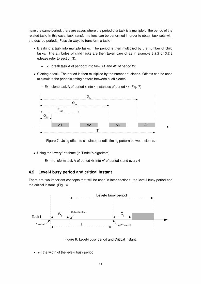
have the same period, there are cases where the period of a task is a multiple of the period of therelated task. In this case, task transformations can be performed in order to obtain task sets withthe desired periods. Possible ways to transform a task:
• Breaking a task into multiple tasks. The period is then multiplied by the number of childtasks. The attributes of child tasks are then taken care of as in example 3.2.2 or 3.2.3(please refer to section 3).
– Ex.: break task A of period x into task A1 and A2 of period 2x
• Cloning a task. The period is then multiplied by the number of clones. Offsets can be usedto simulate the periodic timing pattern between such clones.
– Ex.: clone task A of period x into 4 instances of period 4x (Fig. 7)
A1 A2 A3 A4
OA1
OA2
OA3
OA4
T
Figure 7: Using offset to simulate periodic timing pattern between clones.
• Using the ”every” attribute (in Tindell’s algorithm)
– Ex.: transform task A of period 4x into A’ of period x and every 4
4.2 Level-i busy period and critical instant
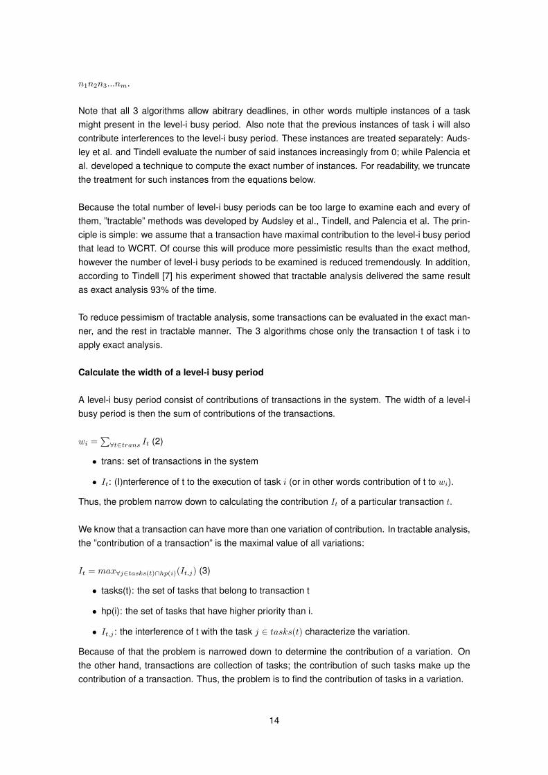
There are two important concepts that will be used in later sections: the level-i busy period andthe critical instant. (Fig. 8)
nth arrival
Task iW
t
n+1th arrivalT
Critical instant
Level-i busy period
Oi
Figure 8: Level-i busy period and Critical instant.
• wi: the width of the level-i busy period
11
• Wt: the phasing between the critical instant and the lastest release of t before the criticalinstant
• t: the transaction task i belong to
• T : the period of t (and task i)
• Oi: the offset of task i
4.2.1 Level-i busy period
Level-i busy period is defined as a continuous time interval [t1, t2) where tasks of lower prioritythan i cannot be activated. In other words, a level-i busy period consist of instances of task i andall the task of higher priority than i. The width of the level-i busy period is an important factor thatwill be used in the algorithm to calculate the corresponding response time of task i.
4.2.2 Critical instant
All response time analysis algorithms start evaluating at the critical instant. A critical instant is thestart of a level-i busy period. Note that the use of offset make it impossible to have a simultaneousrelease of task i and all the higher priority tasks: tasks of the same transaction that have differentoffset may never be released simultaneously. Because of this, a transaction with n different tasksmay have n variations where the release of one of the n task fall into a critical instant (Fig. 9).Thus, multiple critical instants (corresponding to multiple level-i busy periods) exist for a given taski, and response time analysis algorithms for systems with offset begin with finding the right criticalinstant that leads to the worst case response time.
Transaction 1
Critical instant
Level-i busy period
Transaction 2
Transaction 3
Release
End of execution
Figure 9: A critical instant / level-i busy period variation
4.3 Priority assignment
Priority assignment according to rate monotonic or deadline monotonic are found non-optimal forsystems with arbitrary deadline tasks and systems with offset [6]. Audsley derivated an optimal
12
priority assignment algorithm called ”bottom up” [2]; the algorithm is used in all 3 RTA algorithmsmention in section 4.
4.4 The algorithms
The algorithms of Audsley et al. [6], Tindell [7] and Palencia et al. [9] share common pointsin the approach. There are differences in details however, since the algorithms have differentassumptions and constraints. In this section, we will first present the general approach of the 3algorithms. After that, Tindell’s algorithm will be used to demonstrate the approach.
4.4.1 The general approach
Calculate WCRT of a task base on level-i busy periods
The width of the level-i busy period plays an important role in finding the respective task i responsetime. The equation used in the 3 algorithms were something similar to the below:
ri = wi + Wt − aT −Oi (1)
• a: the number of releases of t during the level-i busy period
• ri: the response time of task i
For example, look at Figure 8.
A variation is characterized by a task j which is released at a critical instant. Thus, we can deductthat said task is released right after the phasing Wt (see Figure 8). In other words, Wt = Oj + Jj .
Note that in the case of sporadic transactions, WCRT will only happen when such transactions arereleased at the fastest pace possible (in other words, sporadic transactions are released withoutthe jitters of the events that trigger them) [7].
The worst-case response time Ri is then the maximal value of ri corresponding to the level-i busyperiods. The problem now narrows down to determining which level-i busy periods to examineand how to calculate the width of them.
Which level-i busy periods to evaluate?
We know that in system that make use of offset, multiple critical instants exists. As per the defini-tion, a critical instant is the start of a level-i busy period, so multiple level-i busy periods exists.
Tindell [7] and Palencia et al. [9] proposed ”exact” methods of computing worst-case responsetime. The principle is to examine every possible level-i busy periods - or in other words, to exam-ine every possible combinations of contribution of every transactions. This guarantee to find theexact worst-case response time, but is computational infeasible for non-trivial problems: supposewe have a system with m transactions. Transaction t1 contains n1 tasks, transaction t2 containsn2 tasks and so on. The total number of possible combinations that have to be evaluated is then
13
n1n2n3...nm.
Note that all 3 algorithms allow abitrary deadlines, in other words multiple instances of a taskmight present in the level-i busy period. Also note that the previous instances of task i will alsocontribute interferences to the level-i busy period. These instances are treated separately: Auds-ley et al. and Tindell evaluate the number of said instances increasingly from 0; while Palencia etal. developed a technique to compute the exact number of instances. For readability, we truncatethe treatment for such instances from the equations below.
Because the total number of level-i busy periods can be too large to examine each and every ofthem, ”tractable” methods was developed by Audsley et al., Tindell, and Palencia et al. The prin-ciple is simple: we assume that a transaction have maximal contribution to the level-i busy periodthat lead to WCRT. Of course this will produce more pessimistic results than the exact method,however the number of level-i busy periods to be examined is reduced tremendously. In addition,according to Tindell [7] his experiment showed that tractable analysis delivered the same resultas exact analysis 93% of the time.
To reduce pessimism of tractable analysis, some transactions can be evaluated in the exact man-ner, and the rest in tractable manner. The 3 algorithms chose only the transaction t of task i toapply exact analysis.
Calculate the width of a level-i busy period
A level-i busy period consist of contributions of transactions in the system. The width of a level-ibusy period is then the sum of contributions of the transactions.
wi =∑∀t∈trans It (2)
• trans: set of transactions in the system
• It: (I)nterference of t to the execution of task i (or in other words contribution of t to wi).
Thus, the problem narrow down to calculating the contribution It of a particular transaction t.
We know that a transaction can have more than one variation of contribution. In tractable analysis,the ”contribution of a transaction” is the maximal value of all variations:
It = max∀j∈tasks(t)∩hp(i)(It,j) (3)
• tasks(t): the set of tasks that belong to transaction t
• hp(i): the set of tasks that have higher priority than i.
• It,j : the interference of t with the task j ∈ tasks(t) characterize the variation.
Because of that the problem is narrowed down to determine the contribution of a variation. Onthe other hand, transactions are collection of tasks; the contribution of such tasks make up thecontribution of a transaction. Thus, the problem is to find the contribution of tasks in a variation.
14
The contribution of a task j can be calculated simply by multiplying the capacity of said task Cj
and its number of releases kj during the level-i busy period: kjCj . The number of time a task isreleased during level-i busy period will be the highest when it is first released at the critical instant,in other word:
kmax =⌈W+wi−Oj
T
⌉(4)
when Oj + Jj = Wt = Oi + Ji.
Wt will be used in a ”normalize” function to calculate k from kmax otherwise.
Now we have the equation to calculate the contribution of a transaction:
It =∑∀j∈tasks(t)∩hp(i) kjCj (5)
Note that wi is a function of It (equation 2) and It is also a function of wi (equation 3, 4, 5). We usethe iterative method to calculate the approximation of wi until we have two identical successivevalues, or until we find that the tasks are unschedulable.
4.4.2 Tindell’s algorithm
This section demonstrate the approach of Tindell.
• wi,q: the width of the level-i busy period with q extra instances of task i
• ti: the transaction that task i belong to
• ei: the attribute ”every” of task i
• Ii,t: the total contribution of transaction t to wi,q
• Kj,t: the number of instances of task j of transaction t during wi,q
• vj ; vi,ti: the ”normalize” function to calculate Kj,t from kmax
Tindell’s algorithm to calculate ri starts by selecting the number of extra instances of task i andthe task j (to calculate exact analysis on transaction t):
(6)
Notice that qei +vi,ti is the equivalent of a from equation (1); and Oj +Jj = Wt. To solve equation(6), we need to find wi,q:
(7)
15
Equation (7) is Tindell algorithm’s equivalent of equation (2), with the additional treatment for in-stances of task i. The next problem is to calculate Ii,t:
(8)
(9)
Equation (8) and (9) is Tindell algorithm’s equivalent of equation (4) and (5) respectively. wi,q thuscan be obtained by calculating a series of approximation, until there are two identical successivevalues, or until we find that the tasks are unschedulable.
4.5 Conclusion
In this section we have seen the general approach to RTA with offset of Audsley et al., Tindell andPalencia et al. Due to this, we can predict that the performance of the 3 algorithms would be quitesimilar to each other - the differences would be from how they handle small details, since theyhave different set constraints.
16
5 Implementation and evaluation
In this section, we explain the model design to support the implemenation of the algorithms men-tioned in section 4. We then give the evaluation strategy and the result of evaluating said algo-rithms and implementations.
5.1 The design of Cheddar toolset
The architecture of Cheddar framework consist of two layers: the low-level layer which is ded-icated to data management, and the high-level layer which is Cheddar domain specific. In thesection below, the design decision will have to be implemented in the high-level layer [1].
Cheddar is implemented in a model-driven manner: significant parts of the components in high-level layer are generated from the Cheddar internal models called EXPRESS models. The modelsare written in EXPRESS language.
5.2 Design
To support response time analysis with offset, the EXPRESS models had to be changed:
• Task model: add an offset table and an ”every” attribute. Offset table must be used insteadof a single value to support dynamic offset which can vary in a range.
• Transaction model: a type of Task Group along side with Multiframe (which is outside of thescope of this work).
Figure 10 shows the new EXPRESS models. Offset tables and ”every” were added to existingmodels, while two new models were added: Generic Task Group and Transaction Task Group.
The implementation of the 3 response time analysis algorithms is available in a single Ada pack-age: Feasibility Test.Worst Case Response Time. At the time of writing, only Audsley andTindell algorithms are working correctly. Palencia algorithm still requires further work to make itruns and also support for dynamic offsets are not completed.
5.4 Evaluation
5.4.1 Evaluation strategy
Because the implementation of Palencia’s algorithm isn’t completed, we will only evaluate Audsleyand Tindell’s ones. There are two main criterias to evaluate the algorithms and the implementa-tions: the precision and the performance.
The precision of the algorithms and the implementations are evaluated using the example tasksets that are taken from published papers. Although it would be best to evaluate them with a realusecase of CAN network, we couldn’t get it done within the time limit.
The performance of the implementations are evaluated by benchmarking against large task setsof increasing size.
5.4.2 Evaluating the precision
Example task set #1: Xu and Parnas’
This task set is presented by Xu and Parnas and is claimed that it is unschedulable using eitherfixed or dynamic priority assignment [5].
Table 1: A task set that is unschedulable without offset
The system consists of 5 tasks and 1 transaction. The detail of the tasks are given in the table 1above. The transaction has a period of 161 units of time.
• C: capacity
• D: relative deadline. Bold means the deadline is missed
• O: offset
• Pri: priority (1 is highest)
• r: worst-case response time
18
• rold: response time without the use of offset using fixed priority
This example demonstrates the benefit of using offset: without offset, most of the tasks wouldmiss their deadline - while with offset, all of them didn’t. Task E has its response time reducedby more than half and fits nicely in its deadline. Notice how lower priority tasks benefit more fromoffset than higher priority task.
In this example, both Audsley and Tindell algorithms delivered the same results as in the sourcepaper.
Example task set #2: Audsley’s without task transformation
Table 2: A poorly designed system leads to pessimistic response time
This example is taken from Audsley’s paper about optimal priority assignment [2]. The systemconsists of 6 tasks, belonging to 3 different transactions. Task A and B belong to a transactionwith T = 10; task C belongs to a transaction with T = 20; the rest belong to a transaction with T =40.
This example demonstrates how pessimistic the analysis result can be for a poorly designed sys-tem. Audsley’s algorithm delivered a more pessimistic result than Tindell’s one in this example:with 4 tasks missed their deadlines - comparing to 3 tasks of Tindell.
Example task set #3: Audsley’s with task transformation
Now consider a system that is designed with task transformation. All the task now are groupedinto 1 single transaction with T = 40. The method of task transformation is to clone tasks and givethem the right offsets to simulate their periodic behaviour.
19
Task O D r
A
4 1 114 1 124 1 134 1 1
B
5 2 215 2 225 2 235 2 1
C0 6 6
20 6 6D 7 9 9E 27 14 13F 0 30 30
Table 3: Task transformation makes response time of tasks more optimistic
In this example, both Audsley and Tindell’s algorithms delivered the same results, matching thehand-calculated result in Tindell’s paper [7]. This time all the tasks met their deadlines respec-tively. Notice the huge gain in response time of task E, from 40 reduced to 13 units of time.
5.4.3 Evaluating the performance
51 56 61 66 71 76 81 86 91 96 1010
0.1
0.2
0.3
0.4
0.5
0.6
0.7
Tindell's algorithm
Audsley's algorithm
Number of tasks
Tim
e (
sec)
Figure 11: A performance benchmark using randomized task sets of increasing size
The evaluation process was as below:
1. Generate a random task set of desired size
2. Process the task set 10 times with each algorithm’s implementation
• Measure the time taken each time
• Take the average time
3. Increase the size of the task set and go back to 1.
20
To avoid benchmarking pitfalls, multiple measures were used: A sample task set is evaluatedmultiple of times to eliminate the presence of any external influences. Also the evaluation was notdone with the Cheddar simulation tool but with a simple unit test that make use of the Cheddarcore framework. The reason for doing so is to reduce overhead as much as possible: only theexecution time of the Ada procedure that implement the algorithms are measured.
Because the algorithms were following a general approach to the problem, the curves were of thesame shape (increasing exponentially). Audsley’s algorithm however showed that it is faster thanTindell’s one most of the time, while can be more pessimistic (refer to section 5.2.2).
5.5 Conclusion
There are two things that make a good software: its design and its implementation. In this sec-tion we have seen that Audsley and Tindell algorithms are, by giving the same result as in theiralgorithm’s respective publications, working as expected. Audsley algorithm is known to producea more pessimistic result than Tindell algorithm in some cases, however it is not clear if that is theexpected result. The benchmark however, showed that Audsley algorithm is always faster thanTindell algorithm.
Further investigation might be required, as well as an evaluation against a real usecase of CANnetwork.
21
6 Conclusion and future work
We have implemented response time analyis algorithms with offset into Cheddar, and have ver-ified their precision and performance. In hindsight, in this work we didn’t really tackle distributedsystem nor CAN network - we have implemented algorithms that are compatible with them in-stead: tasks having offset relationship with each other might of course be distributed on differentprocessors; scheduling with offset is indeed tranformable into offline scheduling that stay in CANnetwork nodes. This work has laid the foundation for future works in Cheddar.
We have seen that offset can be used to increase schedulability, by negating the traditional criticalinstant. We also have seen what can be done with offset to model differents real-life constraints insection 3. The application of offset is vast; offset support in Cheddar allow users to model morecomplex real-life systems.
As mentioned in section 2, there can be many possible future works for this research. Firstand foremost however, is to complete Palencia algorithm and add support for dynamic offset.After that, we will address pre-analysis system design problems such as providing tools to assistdesigner in assigning offsets and priorities - as this would be in demand. Last but not least, wewould like to seriously tackle the problems of CAN network schedulability analysis.
22
References
[1] F. Singhoff, A. Plantec, P. Dissaux, J. Legrand, Investigating the usability of real-time schedul-ing theory with the Cheddar project, Journal of Real Time Systems, volume 43, number 3,pages 259-295. November 2009. Springer Verlag. ISSN:0922-6443.
[2] N. C. Audsley, Optimal Priority Assignment and Feasibility of Static Priority Tasks With Arbi-trary Start Times, YCS 164, Dept. Computer Science, University of York, 1991.
[3] K. Tindell, H. Hansson, and A. Wellings, Analyzing Real-Time Communications: ControllerArea Network (CAN), Real-Time Systems Symposium, 1994., Proceedings.. IEEE, 1994.
[4] K. Tindell, A. Burns, Guaranteeing message latencies on Control Area Network (CAN), Pro-ceedings of the 1st International CAN Conference. 1994.
[5] J. Xu, D. L. Parnas, On Satisfying Timing Constraints in Hard Real-Time Systems, SoftwareEngineering, IEEE Transactions on 19.1 (1993): pages 70-84.
[6] N. Audsley, K. Tindell, A. Burns, The end of the line for static cyclic scheduling?, Proceedingsof the 5th Euromicro Workshop on Real-time Systems. 1993.
[7] K. Tindell, Adding Time-Offset to Schedulability Analysis Real-Time Systems ResearchGroup, Department of Computer Science University of York, England, 1994.
[8] K. Tindell, J.Clark, Holistic schedulability analysis for distributed hard real-time system, Mi-croprocessing and microprogramming 40.2 (1994): pages 117-134.
[9] J.C. Palencia, M. Gonzalez Harbour, Schedulability Analysis for Tasks with Static and Dy-namic Offsets, Real-Time Systems Symposium, 1998. Proceedings., The 19th IEEE. IEEE,1998.
[10] J. Goossens, Scheduling of Hard Real-Time Periodic Systems with Various Kinds of Deadlineand Offset Constraints, Diss. PhD thesis, Universite Libre de Bruxelles, 1999.
[11] J.C. Palencia, M. Gonzalez Harbour, Offset-Based Response Time Analysis of DistributedSystems Scheduled under EDF, Real-Time Systems, 2003. Proceedings. 15th EuromicroConference on. IEEE, 2003.
[12] J. Maki-Turja, M. Nolin, Faster Response Time Analysis of Tasks With Offsets, Proc. 10thIEEE Real-Time Technology and Applications Symposium (RTAS). 2004.
[13] R. Dobrin, G. Fohler, Implementing Off-line Message Scheduling on Controller Area Network(CAN), Emerging Technologies and Factory Automation, 2001. Proceedings. 2001 8th IEEEInternational Conference on. IEEE, 2001.
[14] A. Choquet-Geniet, E. Grolleau Minimal schedulability interval for real-time systems of peri-odic tasks with offsets, Theoretical computer science 310.1 (2004): pages 117-134.
[15] M. Grenier, J. Goossens , N. Navet, Near-Optimal Fixed Priority Preemptive Scheduling ofOffset Free Systems, 14th International Conference on Real-Time and Networks Systems(RTNS’06). 2006.
23
[16] M. Grenier, L. Havet, N. Navet, Pushing the limits of CAN - scheduling frames with offsetsprovides a major performance boost, 4th European Congress on Embedded Real Time Soft-ware (ERTS 2008). 2008.
[17] R. I. Davis, S. Kollmann, V. Pollex, F. Slomka, Controller Area Network (CAN) SchedulabilityAnalysis with FIFO queues, Real-Time Systems (ECRTS), 2011 23rd Euromicro Conferenceon. IEEE, 2011.
[18] P. M. Yomsi, N. Navet, R. I. Davis, Controller Area Network (CAN): Response Time Anal-ysis with Offsets, Factory Communication Systems (WFCS), 2012 9th IEEE InternationalWorkshop on. IEEE, 2012.