Ressort: An Auto-Tuning Framework for Parallel Shuffle Kernelskrste/papers/EECS-2015-246.pdf ·...

Ressort: An Auto-Tuning Framework for Parallel

Shuffle Kernels

Eric Love

Electrical Engineering and Computer SciencesUniversity of California at Berkeley

Technical Report No. UCB/EECS-2015-246

http://www.eecs.berkeley.edu/Pubs/TechRpts/2015/EECS-2015-246.html

December 17, 2015

Copyright © 2015, by the author(s).All rights reserved.

Permission to make digital or hard copies of all or part of this work forpersonal or classroom use is granted without fee provided that copies arenot made or distributed for profit or commercial advantage and that copiesbear this notice and the full citation on the first page. To copy otherwise, torepublish, to post on servers or to redistribute to lists, requires prior specificpermission.

Acknowledgement

This research is partially funded by DARPA Award Number HR0011-12-2-0016, theCenter for Future Architecture Research, a member of STARnet, aSemiconductorResearch Corporation program sponsored by MARCO and DARPA, andASPIRE Labindustrial sponsors and affiliates Intel, Google, Huawei, Nokia, NVIDIA,Oracle, and Samsung. Any opinions, findings, conclusions, orrecommendations inthis paper are solely those of the authors and do not necessarily reflect theposition or the policy of the sponsors.

Ressort: An Auto-Tuning Framework for Parallel Shu✏e Kernels

Copyright 2015by

Eric Love

1

Abstract

Ressort: An Auto-Tuning Framework for Parallel Shu✏e Kernels

by

Eric Love

Master of Science in Computer Science

University of California, Berkeley

Krste Asanovic, Chair

This thesis presents Ressort, an auto-tuning framework for computational patterns thatperform any kind of data-dependent data reordering or transformation. These programs,which we call shu✏e kernels, account for large fractions of the runtime of database work-loads and other applications. Hardware-conscious optimizations of shu✏e kernels are allalike in that they generally consist of choosing one of many possible ways to decomposea particular kernel into a pipeline of more primitive operations: a sort might consist of ahash-based partitioning followed by an in-cache quicksort, or a join might entail sorting andthen merging, for example. Ressort presents a domain-specific language (DSL) that enablesthe succinct expression of these compositions while also exposing the nested array-style par-allelism that they imply, and supplies a compiler to exploit it. It also includes a parallelC-like intermediate representation that assists in the generation of performant shu✏e kernelimplementations. We present the design and implementation of these two language layers,and evaluate the performance of their output on a variety of hardware targets under di↵erentalgorithmic requirements.

i

Contents

Contents i

1 Introduction 11.1 Algorithmic Design Space of Shu✏e Kernels . . . . . . . . . . . . . . . . . . 21.2 Auto-Tuning: High- and Low-level Tuning Spaces . . . . . . . . . . . . . . . 31.3 A Scala-based Framework for Shu✏e Kernel Code Synthesis . . . . . . . . . 4

2 Background 62.1 Fundamental Shu✏e Kernels . . . . . . . . . . . . . . . . . . . . . . . . . . . 62.2 Related Work . . . . . . . . . . . . . . . . . . . . . . . . . . . . . . . . . . . 142.3 Summary . . . . . . . . . . . . . . . . . . . . . . . . . . . . . . . . . . . . . 18

3 The Ressort Operator Functional Language (ROFL) 193.1 A Simple ROFL Program . . . . . . . . . . . . . . . . . . . . . . . . . . . . 193.2 Kinds of ROFL Operators . . . . . . . . . . . . . . . . . . . . . . . . . . . . 203.3 Composing Shu✏e Kernels in ROFL . . . . . . . . . . . . . . . . . . . . . . 233.4 Summary of ROFL Operators . . . . . . . . . . . . . . . . . . . . . . . . . . 26

4 ROFL Compiler Front-End 294.1 Overview . . . . . . . . . . . . . . . . . . . . . . . . . . . . . . . . . . . . . . 294.2 Operator DAGs and Common Subexpression Elimination . . . . . . . . . . . 304.3 Operator Fusion: Exploiting Temporal Locality . . . . . . . . . . . . . . . . 31

5 IRep: A Flexible, C-Like Parallel IR 345.1 Motivation . . . . . . . . . . . . . . . . . . . . . . . . . . . . . . . . . . . . . 345.2 Overview of the IRep Language . . . . . . . . . . . . . . . . . . . . . . . . . 355.3 Language Syntax . . . . . . . . . . . . . . . . . . . . . . . . . . . . . . . . . 365.4 Type System . . . . . . . . . . . . . . . . . . . . . . . . . . . . . . . . . . . 37

6 Experimental Methodology 406.1 Problem Setting and Experimental Parameters . . . . . . . . . . . . . . . . . 406.2 Experimental Setup . . . . . . . . . . . . . . . . . . . . . . . . . . . . . . . . 426.3 Test and Verification . . . . . . . . . . . . . . . . . . . . . . . . . . . . . . . 44

ii

6.4 Measurement . . . . . . . . . . . . . . . . . . . . . . . . . . . . . . . . . . . 46

7 Evaluation: Tuning Results 507.1 Partitioning . . . . . . . . . . . . . . . . . . . . . . . . . . . . . . . . . . . . 507.2 Sorting . . . . . . . . . . . . . . . . . . . . . . . . . . . . . . . . . . . . . . . 547.3 Conclusion and Limitations . . . . . . . . . . . . . . . . . . . . . . . . . . . 567.4 Reflections and Future Directions . . . . . . . . . . . . . . . . . . . . . . . . 57

A ROFL Compiler Front-End: Implementation Details 58A.1 Internal Nested-Array Representations . . . . . . . . . . . . . . . . . . . . . 58A.2 RoflArray Bu↵er Allocation . . . . . . . . . . . . . . . . . . . . . . . . . . . 60A.3 Operator Fusion: Exploiting Temporal Locality . . . . . . . . . . . . . . . . 64

B IRep: Code Transformations and C++ Generation 67

C Code Generation for Shu✏e Kernel Primitives 72C.1 Overview . . . . . . . . . . . . . . . . . . . . . . . . . . . . . . . . . . . . . . 72C.2 Record Streams . . . . . . . . . . . . . . . . . . . . . . . . . . . . . . . . . . 73C.3 Partitioning Primitives . . . . . . . . . . . . . . . . . . . . . . . . . . . . . . 74C.4 Sorting Primitives . . . . . . . . . . . . . . . . . . . . . . . . . . . . . . . . . 75

D Supplementary Performance Data 78D.1 Partitioning Results . . . . . . . . . . . . . . . . . . . . . . . . . . . . . . . . 78D.2 Sorting Results . . . . . . . . . . . . . . . . . . . . . . . . . . . . . . . . . . 83

Bibliography 87

iii

Acknowledgments

I would like first and foremost to thank my advisor, Krste Asanovic, for supporting thisproject consistently from the beginning. More recently, Lisa Wu has contributed countlesshours of advice, assistance, and guidance for which I am very grateful. Many thanks aredue to Scott Beamer, whose tutelage in performance counter interpretation and OpenMPsubtleties was invaluable. Finally, I would like to thank Dave Patterson for very generouslyreviewing this thesis.

This research is partially funded by DARPA Award Number HR0011-12-2-0016, the Cen-ter for Future Architecture Research, a member of STARnet, a Semiconductor Research Cor-poration program sponsored by MARCO and DARPA, and ASPIRE Lab industrial sponsorsand a�liates Intel, Google, Huawei, Nokia, NVIDIA, Oracle, and Samsung. Any opinions,findings, conclusions, or recommendations in this paper are solely those of the authors anddo not necessarily reflect the position or the policy of the sponsors.

1

Chapter 1

Introduction

Software spends a lot of time moving data from one place to another. Operating systemsburn CPU cycles running memcpy() and memset(), while device drivers DMA swathes ofbytes to and fro. Even though optimal implementations of memcpy() are tricky to code,due to the cumbersome quirks of packed SIMD instructions and subtleties of memory accessalignment, the right thing to do for a given machine is generally surmisable.

Databases, more interestingly, spend their time moving records around in ways thatdepend on the contents of the records themselves: they sort them, partition them, buildhash tables, perform joins, apply filters, and perform all manner of other transformations.Many non-database workloads make use of these algorithms too, so their e�ciency is broadlyimportant. However, they are very ine�cient when implemented naıvely, and it is often farfrom obvious what sort of sophistication is needed, or even what the best kind of algorithmis.

Worse yet, all kinds of algorithms for these problems are tricky to optimize because theircommunication patterns cannot be pre-determined. Sorting an array might require movingthe first element to the end, or leaving it in place. This pattern is quite di↵erent frommathematical kernels like matrix multiplication, where the programmer can reason aboutwhich elements combine with which other elements, and can statically order arithmeticoperations so as to maximize the amount of inter-element communication that happensthrough the highest levels of the memory hierarchy.

This type of communication and movement distinguishes shu✏e kernels from other com-putational patterns. We introduce and employ the term shu✏e kernel to designate any kindof data-dependent data reordering, which is the focus of this study. Moreover, we attemptto enumerate the ways in which random interactions between shu✏e kernels’ inputs can beconstrained and managed to achieve high performance on diverse hardware platforms.

This thesis describes specific shu✏e patterns, algorithms, and their design spaces, andproposes a software framework to help programmers uncover the best strategies for any par-ticular circumstance. This framework consists of a compiler for a domain-specific language(DSL) that describes shu✏e patterns as compositions of the algorithmic building blockswe’ve examined.

CHAPTER 1. INTRODUCTION 2

1.1 Algorithmic Design Space of Shu✏e Kernels

Many optimized algorithms have been proposed for each shu✏e pattern in order to overcomethe mismatch between these patterns’ data-dependent data movement and hardware’s abilityto give peak performance only where there is locality and predictability. Decades ago, thismeant minimizing the number of random disk I/Os needed to process a query; now, itmeans avoiding DRAM tra�c, exploiting prefetchers, keeping hardware threads busy, andmaximizing instruction- and data-level parallelism within a core.

Both then and now, a few common themes pervade the space of strategies for mappingshu✏e kernels e�ciently onto the physical reality of hardware:

1. If an algorithm requires too many random accesses to an array, partition that arrayinto sets of related values. For example: hash joins send probes all over a large table,resulting in cache misses or random disk accesses, so instead divide up the inputs basedon high-order bits of their keys and build separate, smaller hash tables for each bin [31,38].

2. When multiple processors are available, divide up inputs among them either by:

a) partitioning the input, as above, and processing partitions independently, (calledpartition-then-split) or

b) by simply dividing up or splitting the original, unordered inputs at will, processingthem separately at each node, and then merging the results at the end to restoreorder (split-then-merge)

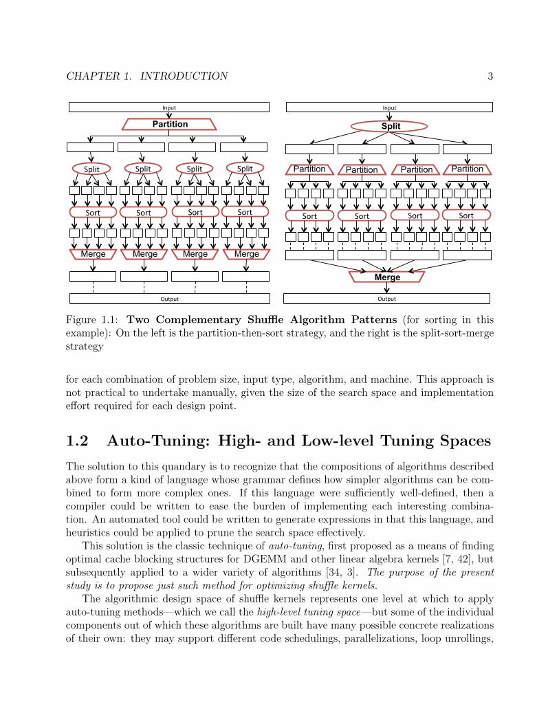
Figure 1.1 illustrates the two structures of (2) as applied to a sorting algorithm. Each halfof the figure actually depicts a combination of the parition-then-split and split-then-mergemethods, applied in a di↵erent order in each case. Both expose parallelism at two levels,and both could themselves be component parts of a still larger operation.

Which strategy is better depends on many aspects of both the target hardware platformand the input data itself. If the data’s keys are not uniformly distributed, partitioning won’tresult in even load balance across processors or cache blocks, but if they are, a large mergemight be slow by comparison. If the target machine has more or fewer levels of parallelism(multiple sockets, cores, SIMD ways, etc.), more or fewer levels of parallelism should beexposed. If the memory system of the machine in question has high write bandwidth orcan better tolerate random accesses than another, then the e�ciency of a higher-fanoutpartitioning might change the tradeo↵ too.

One generalization holds across all these cases: the most e�cient implementation ofany shu✏e pattern on a particular platform will be a recursive composition of partitions,merges, and smaller instances of the target pattern. However, given the large number offactors on which the optimum choice depends, it is di�cult to predict which combinationof strategies is optimal. Ideally, then, we would like to find the best algorithm empirically,but that would require codes with quite di↵erent structures and expressions of parallelism


Split Split Split Split

Sort Sort Sort Sort

Output

Input

Sort Sort Sort Sort

Output

Input

Partition Split

Merge Merge Merge Merge

Merge

Partition Partition Partition Partition

Figure 1.1: Two Complementary Shu✏e Algorithm Patterns (for sorting in thisexample): On the left is the partition-then-sort strategy, and the right is the split-sort-mergestrategy

for each combination of problem size, input type, algorithm, and machine. This approach isnot practical to undertake manually, given the size of the search space and implementatione↵ort required for each design point.

1.2 Auto-Tuning: High- and Low-level Tuning Spaces

The solution to this quandary is to recognize that the compositions of algorithms describedabove form a kind of language whose grammar defines how simpler algorithms can be com-bined to form more complex ones. If this language were su�ciently well-defined, then acompiler could be written to ease the burden of implementing each interesting combina-tion. An automated tool could be written to generate expressions in that this language, andheuristics could be applied to prune the search space e↵ectively.

This solution is the classic technique of auto-tuning, first proposed as a means of findingoptimal cache blocking structures for DGEMM and other linear algebra kernels [7, 42], butsubsequently applied to a wider variety of algorithms [34, 3]. The purpose of the presentstudy is to propose just such method for optimizing shu✏e kernels.

The algorithmic design space of shu✏e kernels represents one level at which to applyauto-tuning methods—which we call the high-level tuning space—but some of the individualcomponents out of which these algorithms are built have many possible concrete realizationsof their own: they may support di↵erent code schedulings, parallelizations, loop unrollings,


OperatorExpression

Front-EndCompiler

IR

IRTranslator

BackendCompiler

C++/asm/LLVMIR

op.o

ProblemSpec

Tuner

TestInputs(RelaBons)

RunBmeLibraries

TestHarness

Performance&DataResults

Compiler Plane Tuner Plane

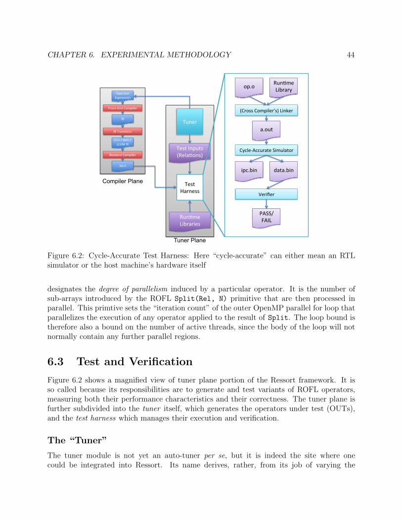
Figure 1.2: Ressort Compilation and Testing Loop

and so on. We call these parameters the low-level tuning space. To obtain real e�ciency,tuning must be applied at both levels.

1.3 A Scala-based Framework for Shu✏e Kernel CodeSynthesis

This thesis presents Ressort1, an auto-tuning framework for shu✏e algorithms that spansboth the high- and low-level design spaces. Figure 1.2 shows its organization. It comprisesboth a compiler plane, which generates code for di↵erent structural decompositions of shuf-fle algorithms, and a tuner plane, which generates these decompositions, and measures theperformance of the compiler’s output. Within the compiler plane, two domain-specific lan-guages support tuning across both levels of design space. The Ressort Operator FunctionalLanguage (ROFL) expresses the algorithmic design space of Section 1.1, while the Ressortintermediate representation IRep supports parameterized code generation for each primitivealgorithm implemented by ROFL.

1 The name Ressort is intended to be read either in English as /ô@soôt/ or in French as /K@sOK/ (“spring,resilience”)


Ressort’s goal is to enable rapid evaluation of many di↵erent structural variants of shuf-fle algorithm implementations. While it does not yet interface with any external machinelearning-based optimization or search tool, it does grant the programmer a means of quicklyand concisely expressing any desired kernel decomposition, and of generating fast parallelcode to implement that decomposition. The contributions of this paper are therefore:

• ROFL: a new DSL for describing shu✏e patterns in a way that exposes their inherentparallelism

• A compiler for the ROFL language that emits parallel OpenMP/C++ code

• IRep, a C-like intermediate language that facilitates low-level tuning and code trans-formations inside the ROFL compiler

• An architectural study that characterizes the performance tradeo↵s of ROFL primitiveoperations, and more complex algorithms built from them, on several diverse hardwareplatforms

The rest of this thesis is structured as follows: Chapter 2 reviews the fundamental algo-rithms out of which shu✏e kernels are assembled, introduces a taxonomy of algorithms builton top of them, and discusses prior work on optimizing them. Chapter 3 presents the ROFLlanguage as a Scala-embedded DSL, and shows how it can be used to construct performantshu✏e algorithms for a variety of purposes. Chapter 4 examines the compiler we have builtfor the ROFL language, while Appendix C describes how it implements each primitive algo-rithm individually. Chapter 5 presents the IRep intermediate language, explaining its designdecisions and its translation to C++. Finally, Chapters 6 and 7 analyze the performance ofthe ROFL compiler’s output for sorting and partitioning on several di↵erent platforms.

6

Chapter 2

Background

This chapter surveys the space of shu✏e kernels, reviews the various algorithms proposed fortheir implementation, and discusses previous work on optimizing their performance throughhardware and software means.

2.1 Fundamental Shu✏e Kernels

In this section we review the most fundamental building blocks of shu✏e kernels, and discusstheir implementation, parallelization, qualitative performance characteristics, and memoryoverheads. Our discussion follows the taxonomy of algorithmic primitives given in Figure 2.1.It is these units which Chapter 3 explicitly composes to form complex, performant operators,but we simply note that any of the partitioning algorithms (green) can serve as inputs to asort algorithm (red), and both of those may appear in a complex join (purple).

Notation

The descriptions of shu✏e kernels throughout the rest of this section all assume a relationconsisting of an array of records is to be reordered or manipulated in some way. Here the termrecord refers to some bytes of data in an arbitrary format of which some bits are designatedas the key. Most shu✏e kernels concern only the key bits of each record, which determinewhere that record is to be relocated to or how it generally is to be treated. Within a givenrelation, all records are assumed to have the same data type, and have the same subset ofbits used as the key.

The following variables and abbreviations are assumed throughout the rest of this dis-cussion:

• R, R1

, R2

, etc. represent relations used as input to some shu✏e algorithm

• |R| is the number of records contained in relation R

• R[n] is the nth record of relation R

CHAPTER 2. BACKGROUND 7

Shuffle Algorithms

Partition

Radix Range

Histogram

Write-Buffered Direct

Chained

In-place Out-of-place

Join

Compound Hash Table Nested Loops

Sort-Merge Partition-Hash

Sort

Primitive Compound

Insert/Select/etc.

SIMD Bitonic

Merge/Quick Radix

MSB-Directed

LSB-Directed

Figure 2.1: A Taxonomy of Shu✏e Algorithms: Partitioning (green), sorting (red), andjoins (purple) form the three main categories of shu✏e algorithms. The leaf nodes of thepartitioning branch can be fed into some members of the sort branch, and building blocksfrom both of these categories can be used to perform a join.

• K(R[n]) is the key of record R[n]

• b is a number of radix bits used in a radix sort or partition

• T is the number of threads used in a parallel algorithm

Partitioning

Partitioning is arguably the most important shu✏e kernel. It divides input records intoseparate buckets or partitions based on the value of some bits of their keys. This kernel is apreliminary step in some possible implementations of all shu✏e patterns, including sorting,joins, hash table building, and many others.

Types of Partitioning

Radix- vs. Range-Based Partitioning can be either range-based or radix-based. Range-based partitioning uses a sorted array of splitter values or delimiters, and assigns records tobuckets defined by the range of keys between any two consecutive splitter values. Radix-based partitioning simply examines a fixed subset of each key’s bits to assign its bucket. Thenumber of bits examined is called the radix.

Histograms vs. Chaining In both radix- and range-based partitioning it is necessary todetermine how much memory is reserved for each output partition. This reservation cannot


be known a priori, so either (1.) partitions must be allowed to expand dynamically by addingnew blocks of records to a linked list or other expandable data structure, or (2.) the inputrelation must be read twice: once to determine the sizes of each partition, and once more toactually move the records. The former is called chaining because it chains together blocksof records for each partition, while the latter is called histogram-based because it constructsa histogram that counts partitions’ sizes.

We presently consider only histogram-based radix partitioning. Although range-based par-titioning is an important component of many algorithms, we defer its investigation to futurework. We also postpone consideration of chaining because it complicates code generation.

Parallelization

Partitioning is inherently parallelizable. Since no inter-record comparisons are needed, allinputs are read and examined independently from each other. Synchronization is only neededto ensure threads output records to disjoint regions of each bucket. In a histogram-basedmethod, this can be done two ways: the shared histogram approach requires an e�cientatomic increment so that threads can update histogram counters safely and independently,while a shared nothing approach creates a separate histogram for each thread, and determinesper-thread partition sizes during the initial counting phase. Shared histograms do not scalewell, and few hardware platforms support suitably e�cient atomics, so we consider onlyshared-nothing algorithms.

Algorithm 1 on the next page gives a complete definition of the shared-nothing parallelhistogram-based radix partition algorithm employed all throughout this study. It consists offour main steps:

1. Histogram counting (lines 2 to 10): Build a histogram array for radix r of size 2r⇥Tand count the number of records in each partition for each thread

2. Prefix sum reduction (lines 11 to 18): Do a prefix sum operation to transform theper-partition counts into o↵sets at which each of the per-thread partitions start

3. Record Movement (lines 19 to 28): Read through all the input records a second timeand write them to their corresponding partitions at the o↵sets given by the histogram

4. Histogram Merger (lines 29 to 33): Merge together the per-thread histograms intoone unified view to return

Computational Characteristics of Partitioning

Partitioning is a computationally inexpensive kernel. It requires only a few tens of instruc-tions per record on most architectures, and has completely regular control flow. Its perfor-mance is constrained mainly by memory bandwidth and, at high radices, scattered writes


Algorithm 1 Parallel Radix Partitioning

1: procedure RadixPart(R, msb, lsb, T )2: r msb� lsb3: Hist[0..T ][0..2r] 04: for t < T do . Build a Histogram5: for i < |R|/T do6: rec R[i+ t|R|/T ]7: part K(rec)[msb : lsb]8: Hist[t][part] Hist[t][part] + 19: end for10: end for11: a

1

, a2

0 . Perform a prefix sum reduction across all threads’ private histograms12: for p < 2r do13: for t < T do14: a

1

Hist[t][p]15: Hist[t][p] a

2

16: a2

a1

17: end for18: end for19: Output[0..|R|] ; . Distribute records to their corresponding partitions20: for t < T do21: for i < |R|/T do22: rec R[i+ t|R|/T ]23: part K(rec)[msb : lsb]24: o↵set Hist[t][part]25: Output[o↵set] rec26: Hist[t][part] o↵set + 127: end for28: end for29: Hist0[0..2r] 0 . Merge together per-thread histograms30: for 1 < i < 2r do31: Hist0[i] Hist[i� 1]32: end for33: Hist0[i] 0 return (Output, Hist’)34: end procedure


distributed randomly across a possibly very large output bu↵er. Section D.1 describes thisaccess pattern in more detail, and presents a simple analytic model for the amount of DRAMtra�c generated by partitioning.

The write pattern exhibited by the record distribution stage of the partitioning algorithmcan be thought to consist of 2rT independent streams : within each thread’s share of eachpartition, the next record is always written to the next sequential address, but these streamsadvance independently of each other, and the next stream to be used is determined randomlyby the key of each input record.

Since for large relations these streams will be distributed evenly across a large virtualaddress space, the TLB working set size will exceed the hardware’s capacity and TLB misseswill impact performance unless large pages are employed. High-radix partitioning’s randomwrite pattern also increases last-level cache (LLC) misses by lowering the likelihood thata given cache line in the output bu↵er, when read in from DRAM on a write miss, willbe written to again before it is conflict-evicted by another stream that maps to the sameset. For this reason, it is sometimes optimal to allocate an output bu↵er that contains onecache line worth of records for each stream in a contiguous array [24]. Only when a linein this bu↵er is completely filled will it then be written to the main output. Another wayto mitigate the impact of high-fanout is to perform partitioning in multiple passes, whereeach pass uses a radix that is a fraction of the final desired one. This compromise requiresscanning the input relations multiple times, but avoids to problems of high fanout.

Sorting

That sorting is fundamental not just within shu✏e kernels but among all algorithms isattested to by the long list of methods commonly taught to undergraduates: quicksort,merge sort, heap sort, insertion sort, radix sort, and so on [14]. In the space of shu✏ealgorithms, sorting’s importance is even greater, since it is a building block of many otheroperations one might wish to implement. It is the first step of a sort-merge join, a componentof set intersection, and in the case of recursive algorithms, one sort’s output is an input toanother.

The space of all possible sorting algorithms is much too vast to review here; instead, wemerely make note of those most relevant to Ressort’s currently supported library of shu✏ekernel primitives, and those it is likely to support soon.

Two Kinds of Sorts

Sort algorithms are traditionally categorized as either comparison-based or not: insertionsort and merge sort compare pairs of values and reorder them accordingly, whereas radixsort never explicitly compares anything with anything else.

In the context of Ressort, we consider two other broad classes of sorting algorithms:(1.) leaf-node sorts, or primitive sorts, and (2.) composite sorting algorithms. The formerclass includes those algorithms which most e�ciently process small (order ten or so) input


elements, and so might serve as building blocks to algorithms in the latter category, whichemploy some strategy to break up their inputs into smaller chunks, and then eventuallyinvoke a primitive algorithm when these chunks are su�ciently small. Thus, we would saythat the primitive algorithms reside at the “leaf nodes” of those composite algorithms’ callgraphs.

Leaf-node Sorts

Among the more primitive kinds of sorts are insertion sort, which has asymptotically quadraticruntime but requires fewer operations at small problem sizes than do more complex meth-ods. We include it as a candidate primitive algorithm in our study for just this reason, anddiscuss its computational properties elsewhere (Section C.4 and D.2). It is often used at thelower levels of recursive algorithms like merge sort, and the size at which to switch over toinsertion sort is a tuning parameter of such algorithms.

Sort networks, such as bitonic or Batcher sort [6], o↵er an alternative strategy for smallinput sizes. These exploit the fact that some algorithms such as merge sort can be madeto have a fixed set of comparisons that does not depend on the values of the input data,and so all these comparisons can be spelled out in advance of execution, either as explicitlyparallel hardware, or as static software instructions. Though they require more total workthan other algorithms, they are valuable for their parallelizability. Recent work has shownsuch algorithms to be amenable to implementation with SIMD instructions [24, 36].

Composite Sorts

Composite sorting algorithms are those that chain two or more primitive algorithms to-gether. We further divide composite sorts into two categories: split-merge and partition-sortalgorithms.

Split-merge sorts are those that first break up their inputs in a data-independent manner,sort all segments independently, and then merge them together somehow. Classical mergesort is in this category: implementations might sort chunks of ten records with insertion sort,and then merge them together. Another example would be cache-blocked radix sort, whereininputs are first evenly divided into cache-sized blocks, each of which is then sorted withradix sort independently before being merged with the other sorted blocks. Partition-sortalgorithms, on the other hand, apply a data-dependent partitioning operation (Section 2.1)to their inputs, and then sort the resulting partitions without the need for a final mergestep. Quicksort is a partition-sort, because it first range-partitions its input by comparingall keys to a splitter value, and then independently sorts the resulting sets.

A special case of partition-sort algorithms is radix sort, which radix-partitions its inputrepeatedly until all bits of the input keys have been used. Radix sort (described moreformally by the program listing in 3.4) has itself two variants. In LSB sort, records arepartitioned first using the least significant bits and then re-partitioned using successivelymore higher-order bits. The partitioning must be stable in this case, meaning that records


sent to the same partition appear in the same order with respect to each other in the outputas they did in the input. By contrast, MSB sort begins partitioning at the most significantbits, and subsequently sorts each resulting partition in parallel. The partitioning operatorneed not be stable.

One additional—and orthogonal—dimension along which composite algorithms may becategorized is whether they are dynamically-structured or statically-structured. Dynamicallystructured algorithms follow a divide-and-conquer strategy and recursively assemble sortedsub-problems until the entirety of the input has been processed. They can react to situationswhere one sub-problem is too large (resulting in load imbalance) by dynamically recursingonce more to split it it up. Statically-structured algorithms determine the number and orderof processing of sub-problems in advance.

Merge sort is always implemented as a dynamically-structured algorithm, but doesn’thave to be: insertion sort-sized sub-arrays could all be sorted at once, and then a fixed-depth merge tree could be imposed on top of them. Radix sort is statically-structured bydefinition, but radix-partitioned radix sort could be implemented dynamically to continuepartitioning some buckets that, due to key skew, are too large to fit in the intended level ofcache. Quicksort is a dynamically-structured partition-sort algorithm, and cannot be madestatic, since the recursive call tree’s structure is data-dependent, unlike merge sort’s, whichdepends only on the size of the input. Sort networks are always statically-structured andcannot be made dynamic.

Computational Characteristics of Sort Algorithms

In general, split-merge algorithms di↵er from partition-sort algorithms in that they tradeo↵ increased computational intensity for better memory hierarchy interaction. Partition-sort algorithms usually incur the wasted memory bandwidth of random accesses when theinputs are large and the radix is high, but execute few dynamic instructions per record andprovide ample parallelism. Split-merge algorithms start o↵ naturally cache-blocked, and onlyever need to make sequential memory accesses, but they require asymptotically more work(O(n log n) vs. O(n)) and have less parallelism in the final merge stages.

Dynamically-structured algorithms like merge sort can be naturally cache-oblivious [18],as they maintain cache-sized working sets without needing any explicit blocking. They areless sensitive to input skew and achieve better load balance, but not all desirable algorithmscan be dynamically structured.

For small input sizes, which can be processed entirely in cache, comparison sorts stresscore microarchitecture with data-dependent branches and stores to the same address withdi↵erent data on the taken and not-taken branch paths. Non-comparison sorts do not havethis problem. Some comparison sorts can be implemented with predicated or conditionalmove instructions to avoid incurring load-store ordering misspeculations.


Joins

Though we do not investigate them in the present study, joins are some of the most commonoperations in analytic database systems, and account for more than half of all execution timein many queries [19]. They are almost always implemented with composite algorithms of thekind described above, so we review their design space here briefly. Formally, a join specifiesthe computation implied in Definition 1:

Definition 1 A join R ./ S of an outer relation R onto an inner relation S is the set of allpairs of records (ri, sj) 2 R ⇥ S such that ri and sj have keys that match. If the conditionfor a match is that the keys are equal, it is called an equijoin.

The simplest way to find all pairs of tuples that meet Definition 1 would be to compareeach record in the outer relation to each record of the inner relation and output those pairswhose keys match. This method is known as nested loops join (NLJ) and requires O(N2)comparisons for two relations of approximately equal length N , so di↵erent methods arerequired for all but the very smallest relations.

The most common form of join for larger input sizes is the hash join, which is so calledbecause it entails building a hash table of the inner relation, and then probing it with recordsfrom the outer relation. The hash join reduces the asymptotic complexity toO(N), but is stillsub-optimal on real hardware. In fact, it shares many of the same bottlenecks as partitioning:if the number of entries in the hash table is too high, then random probes to a large hashtable will frequently miss in cache [38]; if it is too small, then a large constant will be hiddenin the asymptotic bound because collisions will result in more comparisons on every probe.

As a result, two main categories of improved join algorithms have emerged: partitionedhash joins and sort-merge joins. In the case of the former, both input relations are first radix-or range-partitioned with the same partitioning function, and then much smaller hash tablesare built from the partitions of the inner relation, each one of which is probed only withrecords from its corresponding partition in the outer relation. In the case of a sort-mergejoin, both relations are first sorted, and then scanned sequentially in tandem. Whenever thekey of a record in the inner relation is found to be greater than that of the currently-examinedrecord in the outer, the scan pointer in the outer is advanced by one. By maintaining theinvariant that records examined in the inner relation always have keys less than or equalto the scan pointer in the outer relation, it is guaranteed that all possible matches will befound.

The ensemble of techniques proposed in these last two methods shows the relevance ofour compositional approach to the problem of joins. A partitioned hash join composes apartition operator with a hash table build and a probe (really nested loops join), the lattertwo stages of which may proceed in parallel for each of the initial partitions. In a sort-merge join, any of the compound sort techniques presented above—including those whichthemselves utilize partitioning—may serve as the input to the join.


2.2 Related Work

We briefly review some of the literature associated with the main areas of work related toRessort: in-memory databases, shu✏e algorithm optimization and hardware acceleration,software auto-tuning, and parallel programming language systems.

Parallel, In-Memory Database Systems and Query Compilation

Ressort’s very existence is predicated on the emergence of memory-resident, data analytics-oriented column store database systems. Since nearly a decade ago, researchers have focusedtheir attention on the technical challenges that have resulted from the desire to run databasesentirely out of main memory, which fundamentally altered the nature of performance bottle-necks. Instead of minimizing the number and frequency of disk I/Os, engineers now neededto make more e�cient use of CPU and cache hierarchy resources. Additionally, the compute-intensive and mainly read-only queries typical of this new era motivated a shift away fromoptimizing transaction throughput and towards accelerating large aggregation operations onvast tracts of data.

C-Store [40, 26] was one of the pioneering database architectures developed in responseto these trends. It proposed organizing relations in columns rather than rows. This layoutarranges each table as several separate arrays in memory, each one of which contains a singleattribute for all records. This facilitated the parallelization of databases across clusters ofnodes, allowing a single node to contain all entries of a particular column and, potentially,to examine them all at once without intervening communication. Other modern column-stores, such as MonetDB [12, 47, 48], have exploited the columnar organization to findintra-node parallelism. Whereas traditional query execution engines relied on a “tuple-at-a-time” approach that interprets entire queries for a single record before processing another,columnar storage enabled vectorized1processing, or the evaluation of a single operator acrossa block of records at a time. This eliminated interpretive overheads and exposed instruction-level parallelism (ILP) to the compiler and to superscalar architectures.

Other researchers have also sought to improve ILP and general computational e�ciencyin analytic workloads. Some did so by compiling queries to native machine code insteadof interpreting them dynamically [39, 32]. Meanwhile, Shatdal et al. [38] worried alreadyin 1994 about how best to utilize on-chip caches during query execution. The concernsthey raised reverberate throughout all the algorithmic optimizations described below andthroughout the rest of this thesis.

1This should not be confused with vectorization in the vector architecture sense, which is its own areaof investigation [22].


Shu✏e Algorithms for Modern Architectures

Joins

Many modern shu✏e kernel optimizations build upon early join work from database systemsin the 1980s. Several papers from that decade described how partitioning could be used toreduce disk seeks in hash joins [16, 25], as well as to parallelize them.

Subsequent research has re-evaluated these strategies in the context of modern in-memorydatabases. In 2009, Kim et al. [24] revisited the question of whether hash joins or sort-mergejoins were faster on current hardware. They ultimately concluded that hash joins (based onthe shared-nothing parallel partition method of Algorithm 1) would yield better performancefor the time being, but would fall behind as the compute capacity of CPUs with wide SIMDincreased faster than memory bandwidth. Albutiu et al. [1] also proposed a merge sort-basedjoin algorithm, Massively-Parallel Sort-Merge (MPSM), that specifically targeted NUMAmachines. It works by assigning each socket to sort its local NUMA segment of both inputrelations independently, and then performing a massive merge-join in which each processoraccesses all other sockets’ NUMA domains, but does so sequentially in order to benefit fromprefetching.

Blanas, Li, and Patel then argued [8] that, actually, an even simpler partition algorithmbased on atomic updates to a shared histogram table was more e�cient. Later work byBalkesen et al. [3, 4] contradicted the claims made by both Kim and Blanas: first, they arguedthat sort-merge would only outperform radix-hash if relations were very, very large, andsecond, they determined that the purported performance advantage of the shared histogramapproach arose from the use of pre-sorted data in the inner relation, which eliminated accesscontention [5].

Joins do have inherent data parallelism, and Rich Martin’s 1996 technical report [29]showed how to vectorize them for Cray-style architectures. His algorithm derives from Zaghaand Blelloch’s vectorized radix sort [45]. The latter work proposed a vectorized partitioningtechnique (loop raking) that is stable, meaning that records assigned to the same partitionappear in the same order as they did in the original input relation. LSB radix sort requiresthis property for correctness.

Partitioning

More recent work by Polychroniou and Ross [33] thoroughly examined a wide variety ofradix- and range-partitioning algorithms, contributing to and enumerating an already vasttaxonomy of techniques. In particular, they supply in-place and out-of-place variants ofboth Algorithm 1 and the shared histogram approach presented in [9]. They also explainedhow to exploit SIMD instructions to improve range partitioning performance for small andlarge numbers of delimiter keys. They demonstrated and explained the advantage of rangepartitioning over a radix-based approach when used as an input to subsequent steps of ashu✏e kernel, which is that skewed key distributions are less problematic, and that a carefulchoice of delimiters can ensure consistently cache-sized partitions at the output.


Sorting

Satish et al. made the same argument in [37] and [28] as in their previous join paper [24]that radix sort currently outperforms merge sort, but that the balance will tilt in favor of“bandwidth-oblivious” merge sort as SIMD widths become wider and key sizes increase toaccommodate ever larger in-memory relations. They implemented the then fastest radixsort using an output bu↵er-based (Section 2.1) partition operation, and measured a sortingthroughput of 250M keys/second on a 4-core, 3.2GHz Intel Core i7 machine using 32 bitkeys. They claimed that because radix sort is memory bandwidth-bound, its performancewill not improve on future hardware.

Therefore, they also implemented a merge sort algorithm using a SIMD sorting networkthat achieves roughly comparable throughput to radix sort. Because this method is currentlycompute-bound, and because its bandwidth requirements are much lower than those of radixsort, its performance will dominate on platforms with greater per-core compute resources.Their parallel merge sort implementation builds on a previous algorithm for GPUs [36], andparallelizes the merger of large lists by finding splitter values, as did [17].

In the same paper as their partition study, Polychroniou and Ross also examined how tobuild faster radix and merge sort implementations on top of their new partitioning primitives.They use range partitioning to divide keys evenly across NUMA domains, and then applyMSB-, LSB-, and comparison-based sorts within NUMA partitions. They found that thebest algorithmic decomposition depended on relation size, key size, and skew, even whilethe hardware platform remained constant. We feel this dependency, combined with theirexpansion of an already large taxonomy of operators, motivates the design of Ressort. Asdi↵erent systems o↵er di↵erent balances of compute to memory bandwidth, cache hierarchydesigns, and degrees of data parallelism, the choice of optimal algorithm becomes even lessintuitive. An e�cient means of generating parallel code for many distinct design points willultimately provide the best means of realizing optimal performance on new platforms.

Hardware Support

Other researchers have sought to improve shu✏e kernel performance with the support ofspecialized hardware ranging from general-purpose data parallel processors to fixed-functionaccelerators. Kaldewey et al. presented e�cient hash join algorithms for GPUs [23]. JiongHe, Shuhao Zhang, and others explored the mapping of database systems onto CPU/GPUhybrid platforms [21, 46]. Meanwhile, Timothy Hayes et al. proposed a vector architecturespecifically targeted at improving hash join and sort performance [19]. They also presenteda new vector sort algorithm and supporting instruction set additions designed to avoidduplicating histograms once per vector element during partitioning [20].

Other researchers have proposed fixed-function accelerators for particular shu✏e kernels.Lisa Wu et al. designed the HARP [43] accelerator to speed up range partitioning, andthen integrated it into their Q100 query processing architecture [44]. The latter’s pipelineso↵ered an assortment of dedicated units for di↵erent shu✏e kernel primitives such as filtering,


partitioning, joining, and aggregation, and provided a dataflow programming model forscheduling query execution on top of them.

Auto-Tuning

Origins: Linear Algebra

The idea of using an automated script to empirically choose an algorithm’s optimal imple-mentation on a particular platform arose in the scientific computing community. “Portable,Hi-Performance ANSI C” (PHiPAC) by Bilmes et al. [7] applied this method to matrix mul-tiplication and other numerical kernels in the mid-1990’s. Their software searched the spaceof possible cache-blockings and register panelings for DGEMM, outputting highly stylizedC code for which even the least reliable of compilers could generate performant assembly.Nearly two decades later, improvements in alias analysis have rendered many of these defen-sive coding strategies irrelevant, but the need to automate the search for the best of manystructural code variants remains strong. Subsequent work by Whaley and Dongarra, “Auto-matically Tuned Linear Algebra Software” (ATLAS) was used by several numerics libraries.More recently, the OSKI [41] extended this approach to sparse matrices, and has been widelydeployed.

Auto-Tuning in Other Domains

The auto-tuning methodology has also been leveraged in several domains outside of linear al-gebra. The Halide [35] project defined a DSL for describing stencil operations on neighboringpixels in graphics kernels, and supplied a compiler to produce and evaluate the performanceof di↵erent operator pipeline schedules. Meanwhile, the SPIRAL project’s [34] approach tooptimizing FFTs inspired Ressort’s treatment of shu✏e algorithms. It exploits the fact thatthere are many possible mathematical decompositions of the FFT kernel, and introducesan algebra to express di↵erent points in this space. Part of their auto-tuning process in-volves sampling various such formulae. Ressort’s ROFL language is thus akin to their SignalProcessing Language (SPL).

Parallel Programming Languages and DSLs

Ressort’s ROFL programming language is also very much indebted to NESL [11]. The latterwork presented in the early 1990’s a language for expressing portable parallel algorithms asparallel operations on nested arrays. This facilitated compilation of NESL code to exploithardware ranging from SIMD units accessed with vector instructions up to cluster machinesprogrammed via MPI. The shu✏e patterns targeted by Ressort map very naturally onto thisparadigm, and we hope eventually to cover a similar breadth of scales.

The Ressort compiler’s C++ backend leverages the parallel OpenMP [15] extensions for Cand their accompanying language runtime. The OpenMP framework permits the expressionof thread- and data-level parallelism by parallel regions. When a C++ code block is tagged


with OpenMP’s omp parallel pragma, all threads spawned by the runtime will executethe block concurrently. More importantly, a parallel pragma applied to a for loop indicatesthat there are no dependencies between successive loop iterations, and causes the runtimeto divide the iterations among threads.

2.3 Summary

The three main flavors of shu✏e kernels—partitions, sorts, and joins—have each been thesubject of virgorous investigation, and the simpler implementations of each have been de-ployed in more complex versions of the others. At the same time, architectural and microar-chitectural di↵erences between platorms, as well as di↵erences in the representation, size,and key distribution of relations, can all change the tradeo↵s that make one strategy moreviable than another. We consider these two facts as motivation for the design of a singleprogramming language that compactly expresses shu✏e algorithms and enables algorithmicdesign space exploration on current and future architectures.

19

Chapter 3

The Ressort Operator FunctionalLanguage (ROFL)

As Chapter 1 argues, the most performant implementations of shu✏e algorithms are usuallyrecursive compositions of more fundamental shu✏e operations. Since the best strategy tochoose at each level of composition is non-obvious, as are the optimal number of levels andthe parameters to each level itself, the only way to achieve peak performance on any systemis to experimentally evaluate many di↵erent points in this space. It is the goal of this projectto enable just such a design space exploration. We present the Ressort Operator FunctionalLanguage (ROFL), which allows the compact expression of shu✏e algorithms. It exposesthe nested-array type of parallelism induced by partitioning or slicing arrays of records, butmoves the burden of exploiting it from the programmer to the compiler. By representingshu✏e kernel compositions at a higher level than fully spelled-out C++ code, it allows thecompiler to transform, reorder, parallelize, and fuse together these operations in ways thatwould not otherwise be possible.

This chapter describes the ROFL language in more detail. We implement ROFL as adomain-specific language (DSL) embedded in Scala. Scala’s rich syntax supports adding lay-ers of syntactic sugar to construct ROFL abstract syntax trees (ASTs) directly and withoutthe need for a ROFL-specific parser. Moreover, by hosting it in the same language as itscompiler, we allow for the expression of ROFL program generators that look themselves likeROFL primitive operations but in fact assemble and return more sophisticated compositionsthereof. Instances of this are shown later in the chapter. For now, we introduce the ROFLlanguage with some simple examples.

3.1 A Simple ROFL Program

ROFL allows a programmer or auto-tuner (hereafter the user) to compose operators, whichtransform arrays of records into reordered, and reorganized arrays of the same or otherrecords. Operators are really functions, in the mathematical or functional programming

CHAPTER 3. THE RESSORT OPERATOR FUNCTIONAL LANGUAGE (ROFL) 20

sense, but we use the term operator to avoid confusion with Scala or C++ functions. Theoutput of the Ressort compiler is a C++ function that implements the semantics of itsoriginal ROFL operator on any input arrays passed to it.

The following is the ‘Hello World’ of ROFL codes:

1 val A: Operator = OuterRel // Defined by ROFL to represent an input array

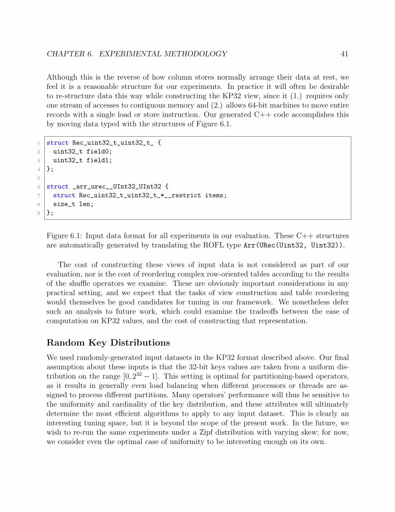
2 val myOp: Operator = Flatten(InsertionSort(Split(A, Length(A)/Const(10))))

These two lines of Scala declare a ROFL operator, myOp:

• Line (1) defines the A symbol to reference a ROFL language primitive OuterRel, whichis itself defined to be the first input array passed as an argument to the C++ functionthat results from compiling this program.

• Line (2) actually specifies an operator to be compiled. Though it may look like a nestedfunction call, it is in fact a declaration of a ROFL AST that Ressort will process later.

Compiling this two-line ROFL program results in the OpenMP-based parallel C++ codeshown in Figure 3.1. More specifically, it generates the InsSrt SplitPar Rel() function,which implements the insertion sort operation in parallel across the Length(OuterRel)/10segments of an input array of records, OuterRel. The auto-generated code is unsurprisinglyobtuse, but its structure is still straightforward:

• Lines (3-7): Allocate a new output bu↵er

• Lines (10-15): Invoke threads to handle segments in parallel

• Lines (33-50): Implement insertion sort with two nested loops

3.2 Kinds of ROFL Operators

A ROFL operator is a combination of one or more ROFL primitives, or operations for whichthe compiler knows how to generate code directly. A simple example is InsertionSort(),which denotes the result of applying the insertion sort algorithm to all the records in itsinput array.

Most ROFL primitives expect as input a flat array of records. Such operators are calledcanonical operators. Whenever a canonical operator receives a nested array as input, animplicit map() operation occurs, and the operator is applied to all sub-arrays independently.By design, these semantics resemble those of map() in functional programming languages,which applies a supplied function to each element of an array independently.

The example in Figure 3.1 describes a computation, or modification of an input array;other primitives imply no computation, but instead specify a change in the structure of their


1 struct _arr_urec__UInt32_UInt32* InsSrt_SplitPar_Rel(struct _arr_urec__UInt32_UInt32* OuterRel)

2 {

3 struct _arr_urec__UInt32_UInt32* r_OuterRel_ref_copy_ptr_0;

4 r_OuterRel_ref_copy_ptr_0 = new struct _arr_urec__UInt32_UInt32;

5 r_OuterRel_ref_copy_ptr_0->len = (OuterRel->len)+((0)*((OuterRel->len)/(10)));

6 r_OuterRel_ref_copy_ptr_0->items =

7 new struct Rec_uint32_t_uint32_t_[r_OuterRel_ref_copy_ptr_0->len];

8 const size_t r_nslice_9 = (OuterRel->len)/(10);

9 const size_t _CTMP1_r_OuterRel_offset_5_max = r_nslice_9;

10 #pragma omp parallel

11 {

12 #pragma omp for

13 for( size_t r_OuterRel_offset_5 = 0;

14 r_OuterRel_offset_5 < _CTMP1_r_OuterRel_offset_5_max;

15 r_OuterRel_offset_5 = r_OuterRel_offset_5+(1))

16 {


18 size_t r_slen_6, r_winsz_7, r_boff_8;


20 size_t r_slen_10, r_boff_12;

21 r_slen_6 = ((OuterRel->len)<r_nslice_9) ?

22 (((OuterRel->len)>(0)) ? (1) : (0)) :

23 (((OuterRel->len)+(r_nslice_9-(1)))/r_nslice_9);

24 r_boff_8 = r_OuterRel_offset_5*r_slen_6;

25 r_winsz_7 = ((r_boff_8+r_slen_6)<(OuterRel->len)) ?

26 r_slen_6 : ((OuterRel->len)-r_boff_8);

27 r_slen_10 = (((OuterRel->len)+((0)*((OuterRel->len)/(10))))<r_nslice_13) ?

28 ((((OuterRel->len)+((0)*((OuterRel->len)/(10))))>(0)) ? (1) : (0)) :

29 ((((OuterRel->len)+((0)*((OuterRel->len)/(10))))+(r_nslice_13-(1)))/r_nslice_13);

30 r_boff_12 = r_OuterRel_offset_5*r_slen_10;

31 const size_t r_isort_numEntries_20 = r_winsz_7;

32 if(r_isort_numEntries_20>(0)) {

33 const size_t _CTMP2_r_isort_i_14_max = r_winsz_7;

34 for( size_t r_isort_i_14 = 0;

35 r_isort_i_14<_CTMP2_r_isort_i_14_max;

36 r_isort_i_14 = r_isort_i_14+(1))

37 {

38 struct Rec_uint32_t_uint32_t_ r_isort_tmp_17 =

39 (OuterRel->items)[r_boff_8+r_isort_i_14];

40 size_t r_isort_j_15 = r_isort_i_14;

41 while( (r_isort_j_15>(0)) &&

42 (((r_OuterRel_ref_copy_ptr_0->items)[r_boff_12+(r_isort_j_15-(1))]).field0 >

43 r_isort_tmp_17.field0))

44 {

45 (r_OuterRel_ref_copy_ptr_0->items)[r_boff_12+r_isort_j_15] =

46 (r_OuterRel_ref_copy_ptr_0->items)[r_boff_12+(r_isort_j_15-(1))];

47 r_isort_j_15 = r_isort_j_15-(1);

48 }

49 (r_OuterRel_ref_copy_ptr_0->items)[r_boff_12+r_isort_j_15] = r_isort_tmp_17;

50 }

51 } else {

52 if(r_isort_numEntries_20>(0)) {

53 (r_OuterRel_ref_copy_ptr_0->items)[r_boff_12] = (OuterRel->items)[r_boff_8];

54 }

55 }

56 }

57 }

58 return r_OuterRel_ref_copy_ptr_0;

59 }

Figure 3.1: Parallel C++ Code generated for ROFL Program in Section 3.1 (withsome manual linebreaks and reformatting to fit this page).


HistRadixPart()

HistRadixPart()

Flatten()

Flatten()

New Buffer New Buffer Same Buffers Input Array

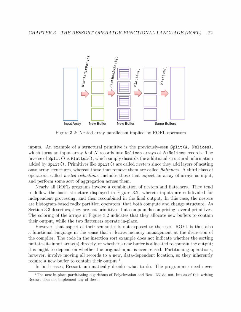
Figure 3.2: Nested array parallelism implied by ROFL operators

inputs. An example of a structural primitive is the previously-seen Split(A, Nslices),which turns an input array A of N records into Nslices arrays of N/Nslices records. Theinverse of Split() is Flatten(), which simply discards the additional structural informationadded by Split(). Primitives like Split() are called nesters since they add layers of nestingonto array structures, whereas those that remove them are called flatteners. A third class ofoperators, called nested reductions, includes those that expect an array of arrays as input,and perform some sort of aggregation across them.

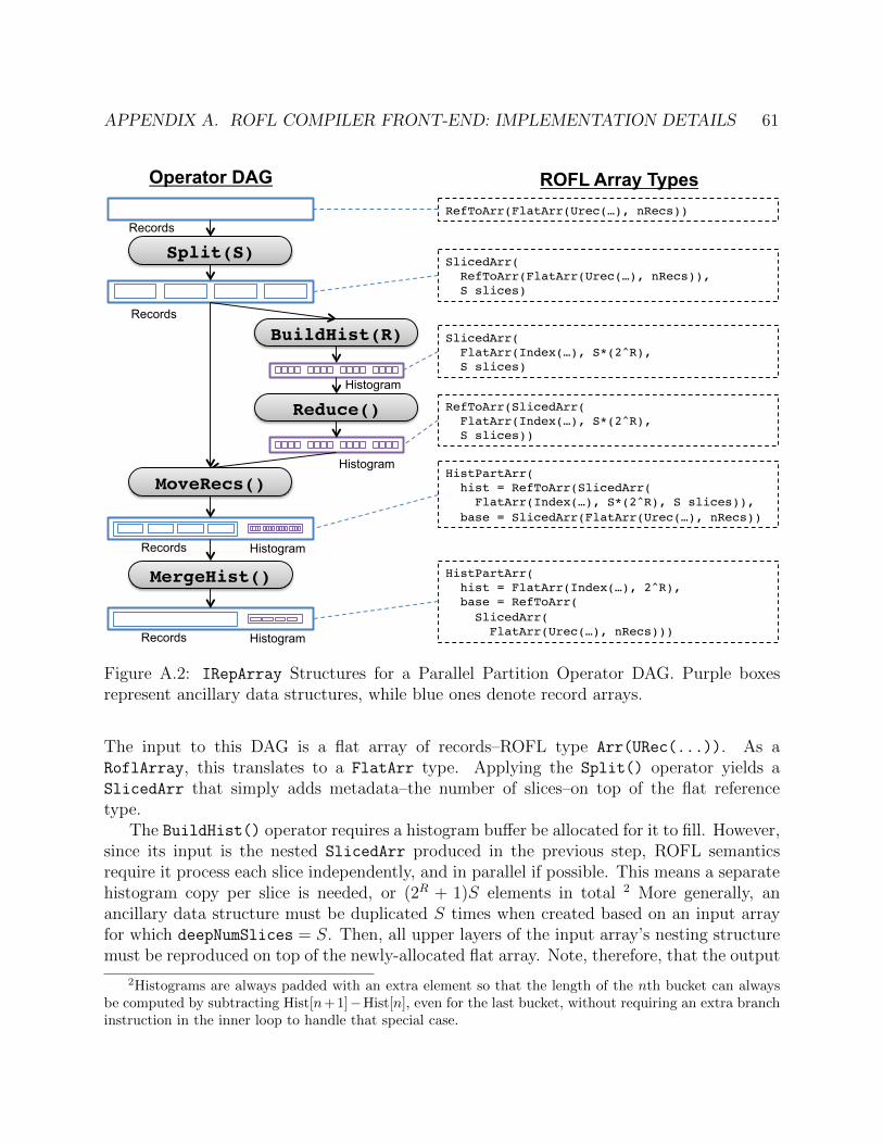
Nearly all ROFL programs involve a combination of nesters and flatteners. They tendto follow the basic structure displayed in Figure 3.2, wherein inputs are subdivided forindependent processing, and then recombined in the final output. In this case, the nestersare histogram-based radix partition operators, that both compute and change structure. AsSection 3.3 describes, they are not primitives, but compounds comprising several primitives.The coloring of the arrays in Figure 3.2 indicates that they allocate new bu↵ers to containtheir output, while the two flatteners operate in-place.

However, that aspect of their semantics is not exposed to the user. ROFL is thus alsoa functional language in the sense that it leaves memory management at the discretion ofthe compiler. The code in the insertion sort example does not indicate whether the sortingmutates its input array(s) directly, or whether a new bu↵er is allocated to contain the output;this ought to depend on whether the original input is ever reused. Partitioning operations,however, involve moving all records to a new, data-dependent location, so they inherentlyrequire a new bu↵er to contain their output 1.

In both cases, Ressort automatically decides what to do. The programmer need never

1The new in-place partitioning algorithms of Polychroniou and Ross [33] do not, but as of this writingRessort does not implement any of these


worry about allocating and freeing bu↵ers, or how many of which type are needed. Evenfor complex operators, the compiler can statically determine most data structure sizes as afunction of the operator’s input size, and consolidate all malloc()s inside a preamble to themain record-processing loops. While it is true that the di↵erent memory overheads imposedby di↵erent algorithms can impact overall performance substantially (especially in systemsthat process multiple queries simultaneously [10]), ROFL still does not directly reveal mem-ory management details because this can simply be “tuned over” as part of the overallperformance, and should a particular design point’s memory overhead limit its through-put, then it will of course be rejected in favor another. In the case of multi-programmeddatabases, Ressort can supply a static estimate of a ROFL operator’s memory footprint tothe query optimizer, which may have more knowledge about the memory and cache footprintsof concurrently-scheduled operations.

Lastly, Ressort leaves unspecified the relative order of execution of di↵erent parts of acompound operator with respect to each other, and so it is also the compiler’s job to schedulecomputation e�ciently when it linearizes the operator DAG (Chapter 4).

3.3 Composing Shu✏e Kernels in ROFL

The real purpose of ROFL is to support the expression of more interesting kernels as com-positions of primitives. These, in turn, can serve as building blocks for larger operators still,and can even be made themselves to resemble primitives by way of syntactic sugar. This sec-tion describes the standard library of ROFL operators, LibRofl. It supplies parameterizedoperator generators for a variety of common tasks, including parallelized radix partitioning,and several types of sorting.

Radix Partitioning

Partitioning is a fundamental step in many shu✏e kernels, and ROFL supplies a suite ofprimitives to support it. It is not itself a primitive because, as Algorithm 1 shows, it com-prises three separate phases and two loops over the input array. Dividing them lets thecompiler schedule them independently2, but this underlying machinery can e↵ectively behidden behind syntactic sugar, as shown in the HistRadixPart() operator of Figure 3.3.

This operator generator will produce di↵erent code depending on the particular choiceof radix bits and specified degree of parallelism. Because many algorithms are built on topof it, Section 7.1 evaluates its performance in isolation, and examines the impact of codegeneration parameters for each of the ROFL primitives that compose it (Section C.2). Later,we show how a simple Scala program can build a radix sort operator out of it.

2There is a serial dependency between them, but the compiler can schedule them relative to otheroperators, that is. A more important reason for the split is actually that they require di↵erent kinds ofbu↵er structures to be allocated for them


1 // Assembles a ROFL radix partition operator on the chosen

2 // bit field of the input keys with the indicated degree of parallelism.

3 def HistRadixPart(base: Operator, lsb: Int, msb: Int, threads: Int): Operator = {

4 // Split the input into ‘threads‘ parallel segments

5 val splitPar = SplitPar(base, Const(threads))

6 MergeHistograms( // Condense per-thread histograms into one

7 MoveRecordsHist( // Distribute records to their partitions

8 splitPar,

9 ReduceHistograms( // Do prefix sum operation

10 BuildHistogram( // Build per-thread histograms in parallel

11 splitPar, // ... parallelism implied by array type!

12 msb, lsb),

13 multi = true), // Indicates parallelized partitioning

14 multi = true)) // (same as above)

15 }

Figure 3.3: Scala/ROFL Code for Parallel Radix Partitioning

Multi-pass partitioning, which can alleviate the performance degradation of high-fanouton some platforms, can be specified in ROFL simply by applying our HistRadixPart()operator to its own output. The only complication is that this results in a nested histogramstructure: if the totally resulting radix of a two-pass partitioning is R = R

1

+ R2

, then therth partition is accessed via a doubly-indirect lookup first of the R

1

MSBs of r and then thesubsequent R

2

bits.3

Sorting

ROFL supplies only a few sorting algorithms as primitives; most actual sort operators areassembled as compositions of sort, split, partition, and merge primitives by Scala-basedoperator generators similar to the one in Figure 3.3. In fact, the only sorting primitivecurrently implemented in the Ressort compiler is InsertionSort, though we imagine addinga SIMD-ized BitonicSort() sort network generator in the future, along with support foran opaque SmallSort() primitive that maps directly to a hardware sort accelerator onplatforms that support it. 4 In this section, however, we examine how to build serial andparallel sort operators out of other ROFL primitives.

3A future version of ROFL should include a “merge histograms upward” operator to eliminate thesuperfluous indirection.

4These could conceivably be calls into vendor-supplied libraries in the case of hardware accelerators, ora Ressort-supplied code generator, in the case of bitonic sort, that resembles those described in Appendix C.


1 // Makes a ROFL operator to perform LSB radix sort on 32-bit keys

2 // by recursively applying partition and flatten operators.

3 def LsbRadixSort(base: Operator, threads: Int, radix: Int): Operator = {

4 // First, handle enough LSBs to make the remaining # of bits

5 // a clean multiple of the radix

6 val rem = 32 % radix

7 val first = if (rem != 0) {

8 HistRadixPart(base, lsb = 0, msb = rem, threads = config.threads)

9 } else {

10 base

11 }

12 // Recursively apply the radix partition operator and flatten

13 def part(base: Operator, lsb: Int): Operator = {

14 if (lsb < 32)

15 part(radixPartOp(base, lsb, lsb+radix-1, threads), lsb+radix)

16 else

17 base

18 }

19 part(first, rem)

20 }

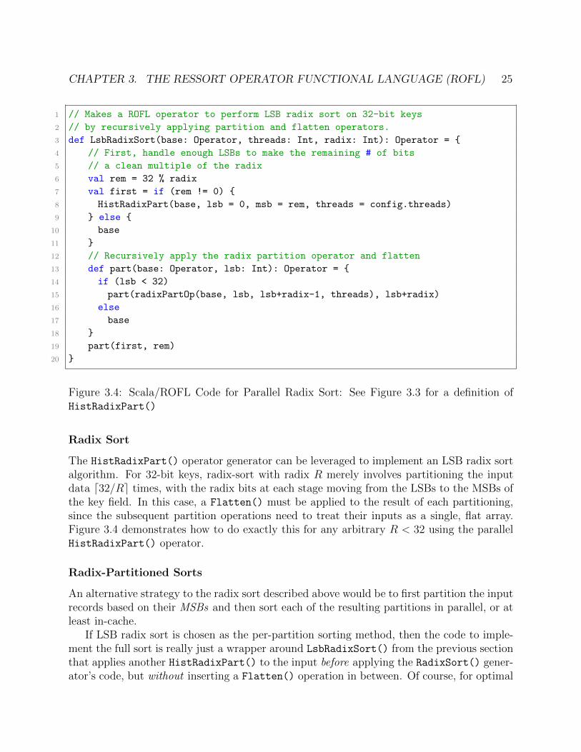
Figure 3.4: Scala/ROFL Code for Parallel Radix Sort: See Figure 3.3 for a definition ofHistRadixPart()

Radix Sort

The HistRadixPart() operator generator can be leveraged to implement an LSB radix sortalgorithm. For 32-bit keys, radix-sort with radix R merely involves partitioning the inputdata d32/Re times, with the radix bits at each stage moving from the LSBs to the MSBs ofthe key field. In this case, a Flatten() must be applied to the result of each partitioning,since the subsequent partition operations need to treat their inputs as a single, flat array.Figure 3.4 demonstrates how to do exactly this for any arbitrary R < 32 using the parallelHistRadixPart() operator.

Radix-Partitioned Sorts

An alternative strategy to the radix sort described above would be to first partition the inputrecords based on their MSBs and then sort each of the resulting partitions in parallel, or atleast in-cache.

If LSB radix sort is chosen as the per-partition sorting method, then the code to imple-ment the full sort is really just a wrapper around LsbRadixSort() from the previous sectionthat applies another HistRadixPart() to the input before applying the RadixSort() gener-ator’s code, but without inserting a Flatten() operation in between. Of course, for optimal


1 def RadixPartInsertionSort(

2 input: Operator, bits: Int, threads: Int): Operator = {

3 Flatten(

4 InsertionSort(

5 HistRadixPart(input, msb=31, lsb=31-bits+1, threads)))

6 }

Figure 3.5: Radix-Partitioned Insertion Sort: Radix partitioning allows insertion sort to beapplied in parallel across partitions.

e�ciency, the LsbRadixSort() code must be modified to avoid redundant partitioning basedon the MSBs, which will be the same for all records within a given partition. ‘LibRofl‘’sactual implementation of these operators does so, and can handle keys with an arbitrarynumber of bits.

The user may also want to set the number of threads requested by LsbRadixSort() toone, thereby letting the number of partitions determine the degree of available parallelism,and giving control over load balancing to the OpenMP runtime. Or the user may exploitthe initial partitioning to obtain LLC-sized partitions, and then sort one partition at a time,but in parallel out of the shared cache. Exploring this design space requires changing just afew lines of Scala/ROFL.

Future Work: Cache-Blocked Split-Merge Sorts

The structural converse of partitioned sorts is the split-merge sort, of which the familiarmerge sort is one example. The algorithms in this family start by dividing their inputs(e.g. with the Split() primitive) into per-thread or per-cache block sub-arrays, sorting thesub-arrays, and then merging those with a merge operator.

Figure 3.6 gives an example from this class of sort algorithms: the cache-blocked radix-merge sort. The CacheBlockedRadixSort() function returns a ROFL operator that dividesits input into cache-size blocks, applies a parallel radix sort to each LLC-sized cache blockin sequence, and then invokes a merge network primitive. We do not evaluate this particularoperator in Chapter 7, however, as the current version of Ressort does not yet include amerge operator.

3.4 Summary of ROFL Operators

Table 3.1 presents a more detailed overview of the various operators that exist in ROFL, aswell as some that are not yet implemented by the compiler but are nonetheless importantparts of the overall algorithmic space targeted by ROFL. In the table, each operator is namedalong with the number and types of its arguments and the type of its output. Types arespecified using a shorthand notation where Arr[T ] designates an array of elements of type


1 def CacheBlockedRadixSort(

2 input: Operator,

3 blockSize: Int,

4 radix: Int,

5 threads: Int): Operator = {

6 MergeSlices( // Builds a merge tree on top of the sub-arrays

7 RadixSort( // Could easily replace with another low-level primitive

8 SplitSeq( // Don’t allow parallel sub-arrays

9 OuterRel,

10 slices = Length(input) / Const(blockSize)),

11 radix,

12 threads))

13 }

Figure 3.6: Cached Blocked Partition and Merge Sort

T , or an array of arrays of type T , up to an arbitrary degree of nesting. As a base type,T simply refers to any kind of record, unless otherwise specified (see Arr[Index] in some ofthe histogram operators, for example). All operator types are specified as functions, since aROFL program is actually a specification of how an input array should be transformed intoan output.

Table 3.1: Summary of ROFL Operators and their Types

Primitive : Type

Description Status

OuterRel : Arr[T ]! Arr[T ]Refers to the first argument (record array) passed to the compiled function Implemented

SplitPar(o, N, [padding]) : Arr[T ]! Arr[Arr[T ]]SplitSeq(o, N, [padding]) : Arr[T ]! Arr[Arr[T ]]

Divides the input array into N arrays of |o|/N elements. If padding is specified, thenas many elements of padding are added between each pair of slices. SplitPar allowsparallel processing of sub-arrays, while SplitSeq does not.

Implemented

Chunk(o, N, [padding]) : Arr[T ]! Arr[Arr[T ]]Divides the input into |o|/N arrays of length N. If padding is specified, then as manyelements of padding are added between each pair of slices.

NOT implemented

InitHistogram(o, msb, lsb, [partitionPadding]) : Arr[T ]! Arr[Index]Initializes a radix r = (msb � lsb + 1) histogram with 2r entries. If padding isspecified, this will produce as many elements of padding between partitions in theresulting bu↵er once records have been moved.

All butpartitionPadding

BuildHistogram(o, hist) : Arr[T ]⇥Arr[Index]! Arr[Index]Reads records in o and increments counters in hist accordingly. Implemented

ReduceHistograms(hist, [multi]) : Arr[Index]! Arr[Index]


Performs a prefix sum reduction on the counters of hist. If multi is set, thenthe histogram is interpreted as a multi-threaded histogram of type Arr[Arr[T ]], andinterpreted appropriately (see Algorithm 1).

Implemented

MoveRecordsHist(o, hist, [padding]) : Arr[T ]⇥Arr[Index]! Arr[T ]⇥Arr[Index]Moves records of the input relation into their assigned partitions according to the o↵-sets contained in the prefix-summed histogram. If padding was set in InitHistogram,then it must be set to the same value here.

Implemented

RestoreHistograms(o, [multi]) : Arr[T ]⇥Arr[Index]! Arr[T ]⇥Arr[Index]Restores all counters in hist to their state before the application ofMoveRecordsHist, which will have incremented each partition’s counter by the num-ber of records it contains. If multi is set, then the multi-threaded histogram case ishandled correctly. Note that o should be an operator containing MoveRecsHist, andits type should be a combination of histogram and bu↵er.

Implemented

Compact(o) : Arr[Arr[T ]]! Arr[Arr[T ]]Produces a new output array where padding in the topmost layer of o has beenremoved.

Implemented

Flatten(o) : Arr[Arr[T ]]! Arr[T ]Removes the outermost layer of array nesting from o. Implemented

MergeSlices(o, [radix=2]) : Arr[Arr[T ]]! Arr[T ]Merges all the (sorted) sub-arrays of o together into one sorted array. We plan togenerate merge trees of arbitrary radix when we implement this operator, meaningthat if o has M sub-arrays, then a tree of depth logM/ log radix will be emitted.

NOT implemented.

Merge(o1, o2) : Arr[T ]⇥Arr[T ]! Arr[T ]Merges the sorted array of o1 with that of o2. NOT implemented.

InsertionSort(o) : Arr[T ]! Arr[T ]Returns the result of sorting o’s array(s) by insertion sort. Implemented

29

Chapter 4

ROFL Compiler Front-End

The front-end is the layer of Ressort responsible for turning a type-checked ROFL operatorinto intermediate IRep code that can then be translated to C++ code. Those latter stagesthat convert IRep to C++ and then compile it are, conversely, called the back-end. Thefrontend’s myriad duties include:

• Turning ROFL operator expressions into operator DAGs

• Annotating DAG nodes with constraints on their scheduling, code generation, andbu↵er allocation

• Allocating and deallocating bu↵er structures for each node

• Finding opportunities to fuse together operators that process the same sub-array struc-tures

• Determining the order in which to execute sub-DAGs relative to each other

• Emitting parallel for loop structures to process sub-arrays independently

• Invoking the appropriate code generator for the ROFL primitive specified at each node

This chapter briefly surveys these phases of compilation, while Appendices A and C describetheir implementation in detail.

4.1 Overview

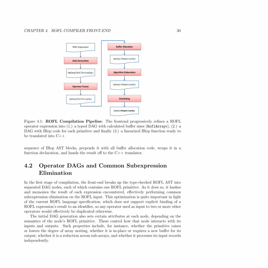
Figure 4.1 shows the front-end pipeline, and the kinds of DAG nodes produced at eachstage. Di↵erent array data types are produced in successive stages as operator primitivesare refined from ROFL into IRep (Section A.1). The ultimate result of this refinement is aDAG containing complete IRep code for each node, along with code to allocate each node’sbu↵ers and metadata. The final stage of the frontend flattens the refined DAG into a linear

CHAPTER 4. ROFL COMPILER FRONT-END 30

ROFL%Expression%

DAG$Genera)on$

OpDag[RoflArrayOp]

Operator$Fusion$

OpDag[RoflArrayOp]

Buffer$Alloca)on$

OpDag[IRepArrayOp]

Algorithm$Elabora)on$

OpDag[IRepArrayOp]

Scheduling$

List[IRepArrayOp]

Figure 4.1: ROFL Compilation Pipeline: The frontend progressively refines a ROFLoperator expression into (1.) a typed DAG with calculated bu↵er sizes (RoflArrays), (2.) aDAG with IRep code for each primitive and finally (3.) a linearized IRep function ready tobe translated into C++

sequence of IRep AST blocks, prepends it with all bu↵er allocation code, wraps it in afunction declaration, and hands the result o↵ to the C++ translator.

4.2 Operator DAGs and Common SubexpressionElimination

In the first stage of compilation, the front-end breaks up the type-checked ROFL AST intoseparated DAG nodes, each of which contains one ROFL primitive. As it does so, it hashesand memoizes the result of each expression encountered, e↵ectively performing commonsubexpression elimination on the ROFL input. This optimization is quite important in lightof the current ROFL language specification, which does not support explicit binding of aROFL expression’s result to an identifier, so any operator used as input to two or more otheroperators would e↵ectively be duplicated otherwise.

The initial DAG generation also sets certain attributes at each node, depending on thesemantics of the node’s ROFL primitive. These control how that node interacts with itsinputs and outputs. Such properties include, for instance, whether the primitive raisesor lowers the degree of array nesting, whether it is in-place or requires a new bu↵er for itsoutput, whether it is a reduction across sub-arrays, and whether it processes its input recordsindependently.


Split(S)

BuildHist(R)

Reduce()

MoveRecs()

MergeHist()Records Histogram

Records Histogram

Histogram

Histogram

Records

Records RefToArr(FlatArr(Urec(…), nRecs))

SlicedArr( RefToArr(FlatArr(Urec(…), nRecs)), S slices)

SlicedArr( FlatArr(Index(…), S*(2^R), S slices)

HistPartArr( hist = RefToArr(SlicedArr( FlatArr(Index(…), S*(2^R), S slices)), base = SlicedArr(FlatArr(Urec(…), nRecs))

HistPartArr( hist = FlatArr(Index(…), 2^R), base = RefToArr( SlicedArr( FlatArr(Urec(…), nRecs)))

RefToArr(SlicedArr( FlatArr(Index(…), S*(2^R), S slices))

Operator DAG ROFL Array Types

Figure 4.2: IRepArray Structures for a Parallel Partition Operator DAG. Purpleboxes represent ancillary data structures, while blue ones denote record arrays.

Figure 4.2 shows the form of this DAG for a parallel partition operator, and indicateswhat kind of array structure is produced by each node. It is during this DAG generationphase that the compiler determines the sizes of all data structures. For example, it infersthat S copies of the histogram are needed as the histogram building operator is applied inparallel to S sub-arrays. It also decides that the output of that node should allocate a newarray for the histogram, while the Reduce() node should re-use its input, as indicated withan explicit reference type. Section A.1 in Appendix A describes these types in more detailand explains how they govern loop generation during algorithm elaboration.

4.3 Operator Fusion: Exploiting Temporal Locality

Ressort exploits nested array parallelism at each DAG node by scheduling that node’s com-putation across each sub-array independently using nested parallel for loops in the IR. A


barrier is thus implied between a node and all nodes from which it receives its inputs (itsparents). This has two important consequences.

First, a child node’s computation cannot be applied to a sub-array immediately when itis produced by a parent, but must wait until all other sub-arrays in the parent have beenprocessed. A single sub-array produced in the parent will likely have been evicted from cacheby the time a child is able to visit it, and no temporal reuse will be exploited.

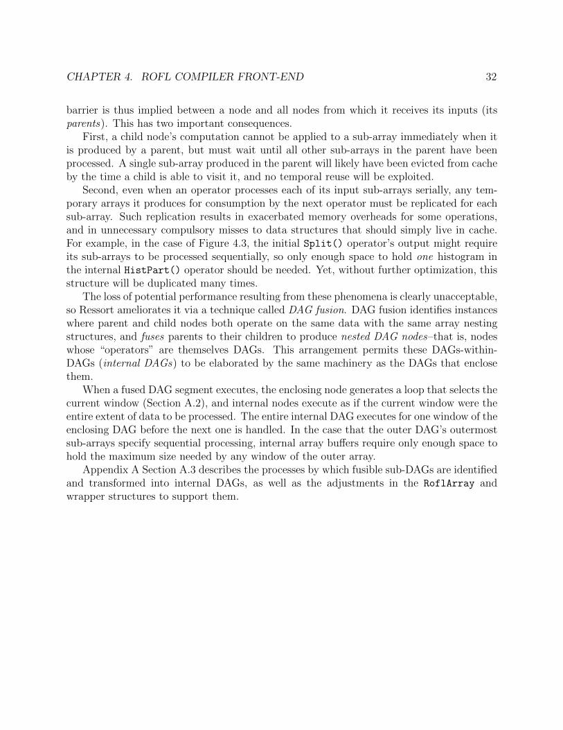
Second, even when an operator processes each of its input sub-arrays serially, any tem-porary arrays it produces for consumption by the next operator must be replicated for eachsub-array. Such replication results in exacerbated memory overheads for some operations,and in unnecessary compulsory misses to data structures that should simply live in cache.For example, in the case of Figure 4.3, the initial Split() operator’s output might requireits sub-arrays to be processed sequentially, so only enough space to hold one histogram inthe internal HistPart() operator should be needed. Yet, without further optimization, thisstructure will be duplicated many times.

The loss of potential performance resulting from these phenomena is clearly unacceptable,so Ressort ameliorates it via a technique called DAG fusion. DAG fusion identifies instanceswhere parent and child nodes both operate on the same data with the same array nestingstructures, and fuses parents to their children to produce nested DAG nodes–that is, nodeswhose “operators” are themselves DAGs. This arrangement permits these DAGs-within-DAGs (internal DAGs) to be elaborated by the same machinery as the DAGs that enclosethem.

When a fused DAG segment executes, the enclosing node generates a loop that selects thecurrent window (Section A.2), and internal nodes execute as if the current window were theentire extent of data to be processed. The entire internal DAG executes for one window of theenclosing DAG before the next one is handled. In the case that the outer DAG’s outermostsub-arrays specify sequential processing, internal array bu↵ers require only enough space tohold the maximum size needed by any window of the outer array.

Appendix A Section A.3 describes the processes by which fusible sub-DAGs are identifiedand transformed into internal DAGs, as well as the adjustments in the RoflArray andwrapper structures to support them.


Split()

Sort()

Flatten()

Flatten()

HistPart()

Sort()

Flatten()

HistPart()

Split()

Flatten()

Figure 4.3: Operator DAG Fusion Example

34

Chapter 5

IRep: A Flexible, C-Like Parallel IR

The output of the frontend compiler is a program that implements the semantics of the orig-inal ROFL expression’s composition of operators. This output is neither machine languagecode nor C++ code. Instead, it is an intermediate representation that is merely very close toC++ code, but which maintains some higher-level semantics and, more importantly, existsas a type-checked AST inside Ressort that can be manipulated and transformed in variousways. The present chapter presents this language, called simply IRep, describing its syn-tax, type system, parallel constructs, and its translation to parallel C++ with OpenMP. Italso discusses a Scala-based interpreter for IRep, which has assisted in debugging the ROFLcompiler and various transformation passes.

5.1 Motivation

Modern compiler backends have at their disposal an arsenal of sophisticated code genera-tion techniques, and make highly performant choices during register allocation, instructionselection, and code scheduling. Ressort leverages this existing work by emitting C++ codeas its final internal level of representation of shu✏e operators, thereby entrusting these verylow-level choices to the complex machinery of GCC and LLVM. However, auto-tuning stilldoes entail forcing the compiler to explore di↵erent points in this space by feeding it withslightly di↵erent input codes. It is therefore desirable to have within Ressort a means ofautomatically transforming C-like code generated by operator elaboration.

This need is common to all auto-tuning systems, which have at some level a C-likeprogram representation that can be programmatically varied. Often this has taken the formof messy string manipulation routines that simply concatenate predefined blocks concreteC code according to some parameter setting. Such systems are brittle, not easily extended,and cannot support code transformations that are independent of the semantics of eachparticular kernel being tuned. They also cannot support operations on code that depend onthe types of variables and expressions.

We have attempted to remedy this state of a↵airs in Ressort by adding a new intermediate

CHAPTER 5. IREP: A FLEXIBLE, C-LIKE PARALLEL IR 35

language, IRep, which is a Scala-embedded DSL for describing C-like programs withoutdirectly spelling out concrete strings of C code. Hosting it in Scala alongside the rest ofRessort allows for the construction of code generators, of which several examples are givenin Appendix C. In this regard it is similar to and inspired by Chisel [2], a DSL developed atBerkeley for writing parameterizable hardware generators in Scala.

Ressort implements IRep by representing and constructing its ASTs directly in Scalaas case classes (pattern matchable recursive data structures), and supplying some syntacticsugar to facilitate the embedding of IRep programs into Scala code. It also supplies a com-plete type-checker for IRep code, and a suite of routines that make it easy to write programtransformations that operate on type-checked ASTs (two are described in Section ??).

A translation layer converts type-checked ASTs into C++ code appropriate for di↵erentcompilation targets and runtimes. Finally, it includes an interpreter that executes IRepprograms directly in Scala.

5.2 Overview of the IRep Language

IRep was designed intentionally to resemble C, into which it is directly translated. It thereforeincludes most of that language’s control flow constructs and data types, including functions,pointers, and structs. Some of these constructs di↵er slightly from their C counterparts in or-der to facilitate the construction of IRep code generators, to prevent unintended emission ofsub-optimal C code, or to maintain higher-level semantics than could otherwise be expressed.The latter category includes parallel for loops, which map directly onto OpenMP equiva-lents. Explicit array operations, such as scans (prefix sum), both simplify ROFL-to-IRepcompilation and enable translators for specific targets, such as GPUs or vector machines,to express those constructs in ways that are most e�cient for those platforms. The rest ofthis section highlights these di↵erences between C’s structures and their IRep homologues,which can be summarized as:

• Expressions do not have side-e↵ects; there is no i++

• Function calls are statements, not expressions; a special assignment statement capturestheir return values

• Loops are always given as a min, max, and stride tuple

• Arrays track their lengths, and always have restrict semantics

• Functions can be nested, but only globals and the formal parameters of the innermostenclosing function are in scope


5.3 Language Syntax

A simple example, culled from the interpreter test suite, serves to introduce the most basiclanguage constructs:

1 val code: IrAst = { // Binds ‘code‘ to the IRep AST at the bottom

2 val f = Id("f") // *Scala* declaration of IRep symbols

3 val x = Id("x")

4 val y = Id("y")

5 // Now IRep code to use them:

6 FuncDec(f, Map(x -> IRInt(), y -> Ptr(IRInt())), {

7 Deref(y) := x * x

8 } ) +

9 DecAssign(y, IRInt(), 0) +

10 App(f, Map( x-> 10, y -> Ref(y)))

11 }

These lines declare a Scala constant code containing an IRep AST that defines a functionf and applies it to a an automatic variable y through a pointer dereference. The firstthree lines inside the AST construction block declare Scala identifiers that stand in for IRepASTs, in this case the minimal expression AST consisting merely of a symbol name (Id()).The function declaration uses a Scala Map[Id, IRType] (mapping from IRep identifiersto IRep types) data structure to describe the types of formal parameters. The () afterprimitive type names declares them as mutable; a trailing (const=true) would do theopposite. Evaluating this code in the interpreter yields a memory state where y is assignedan integer value of 100.

Plenty of syntactic sugar is at play in this example. The assignment in Line (7) exhibitsthree instances: x stands in for Id("x"), x * x is really a Scala call to the overloaded *operator that returns an expression AST, Mul(Id("x"), Id("x)), and an overloaded :=yields an Assign(Deref(Id("y")), Mul(Id("x"), Id("x"))).

All IRep language constructs are introduced in this section with this Scala shorthandnotation, but the above code is indeed the underlying representation. It is also possibleto obtain from the IRep AST implementation a “pretty-printed” form of this code, whichcannot currently be written and parsed directly, but is useful when examining the output ofIRep code generators:

Func f(x: IRInt,y: ptr_IRInt) : {

Deref(y) <--- x*x}var y: IRInt <--- 0f(x=10, y=Ref(y))


Parallel and Sequential For Loops

IRep o↵ers both normal and parallel for loops, and both are more constrained than in C.All for loops must be specified with an explicit induction variable and expressions for aminimum, maximum and stride value. Thus, the upper bound expression will be evaluatedexactly once:

1 val stridedFor = {

2 val sum = Id("sum")

3 val i = Id("i")

4 DecAssign(sum, IRInt(), 0) +

5 ForSeq(i, min=0, max=20, stride=4,

6 (sum := sum + 1))

7 }

Thus, the above code sets sum to five. Constraining for loops in this fashion ensures thatno complex termination predicates will mistakenly emerge increase per-iteration instructioncounts. It also makes it easier to do certain kinds of transformations when the inductionvariable is explicit.

ForSeq specifies an ordinary sequential for loop; ForPar indicates that all loop iterationsare independent and may be executed in parallel.

Functions

IRep also supports functions as a means for operator code generators to encapsulate chunksof reusable logic (the insertion sort “unroller” in Section C.4 is one example). The C++compiler should ultimately inline most of these, assuming -O3 is set, and avoid function calloverhead.

A few features di↵erentiate IRep functions from C++ functions. First, only primitivesmay be passed as arguments—structures are not allowed. Second, because expressions cannothave side e↵ects, return values can only be captured through a special assignment statement,AssignReturn().

Finally, functions are allowed to be nested, which makes them easier to use inside operatorcode generators, as those do not know the surrounding context into which they emit IRepcode. However, as a compromise to simplify C++ code generation, the scope of a function’sbody includes only its formal parameters and global variables; the automatic variables andarguments of any enclosing functions are not visible.

5.4 Type System

In lieu of a formal enumeration of IRep’s type system and typing rules, we simply note wherethese di↵er interestingly from those of C.


Fixed-Width and Machine-Dependent Integer Types

The IRep type system closely mirrors that of the C language. Our intent was to facilitatecompilation into that language and to ensure portability across platforms in terms of bothcorrectness and performance. To that end, IRep supports fixed-width signed and unsignedinteger types at the 8-, 16-, 32-, and 64-bit granularities for storage of record fields requiringa precise width, and architecture-dependent integer types that match the target machine’snative register widths.

Of these, the most important is Index(). It denotes the amount of storage required tohold an index or o↵set into any memory-resident, addressable bu↵er. The Index() type quitenaturally maps onto the C language’s size t data type, and the current compiler alwaysuses it as the type for loop induction variables in array processing loops, for histogramcounter entries, and for all other kinds of array indexing operations.

There is certainly a chance that this conservative representation will waste space if usedto store o↵sets into smaller bu↵ers whose sizes are known statically. Indeed, the impact couldbe particularly acute for frequently-accessed structures (like histograms) that ought to residein the higher levels of the memory hierarchy, and switching to a more compact data typecould improve cachability in such cases. The benefit of marking variables with the Index()type is that it makes them obvious targets for a future compiler analysis pass that woulddown-size whichever indices it can prove are over-provisioned. It is not yet obvious whetheror not it makes sense to generate di↵erent code variants to be chosen among dynamicallyonce the actual sizes of bu↵ers are known. This too is an object of future study.

Arrays

As the purpose of IRep is to represent implementations of array-processing operators, it wasdesigned to make array-handling as straightforward and natural as possible. We do not think,for instance, that it is sensible to make IRep programmers manually maintain variables thattrack the lengths of arrays, as C does, and so IRep arrays do this automatically. Moreover,some common array operations, such as initialization (memset), prefix sum, reversal, and shiftare exposed as explicit language constructs in order to hide target-specific optimizations inthese routines from code generators. It should be the job of the C++ IRep translators todecide whether a given platform is best targeted by parallelization or utilization of dedicatedinstructions.

IRep does not support multidimensional arrays in the same way that C does. Ratherthan standardizing row- or column-major ordering, the language assumes that it is thefrontend compiler’s responsibility to manage data layout in flat bu↵ers. However, it doessupport nested arrays, where all dimensions but the highest consist of arrays of pointers tothe subsequent level’s arrays.


Reference Types

In order to support function calls and structs, IRep includes an explicit Ptr() data type.This is something in between a C-style pointer and a C++ reference, as Ptr-typed variablescan be declared uninitialized, but cannot be cast to an integer, and pointer arithmetic is notsupported. A reference can be acquired to any valid lvalue via the Ref() operator. By fiat,no two references to arrays may alias each other, and the result of doing so is undefined.This restriction allows all arrays to be compiled to C++ arrays with restrict semantics,which enables some compiler operations not otherwise possible under a more conservativeanalysis.

40

Chapter 6

Experimental Methodology

In order to demonstrate the functionality of Ressort, we evaluated the performance of a va-riety of operator compositions across several platforms (Chapter 7). Before presenting thoseresults, we first describe in this chapter the experimental setup used to obtain them, includ-ing the hardware platforms studied, our data-gathering and correctness-checking methods,and our assumptions about the underlying format of input data to all ROFL operators.

6.1 Problem Setting and Experimental Parameters

Data Formats and Memory Layout

KP32: 32-bit Key-Payload Relations

For the purposes of this investigation, we consider only input relations whose records containa 32-bit key and a 32-bit payload, which we refer to as KP32 relations. Although the intendeduse-cases for Ressort—namely, in DBMS query execution engines—will require processingrelations of all shapes and sizes, we restricted the scope of our inquiry to the KP32 classas this represents a useful general-purpose data format that occurs quite frequently in themiddle stages of query processing pipelines, even where the ultimate input or output formatis more complex.

Indeed, a first step in the implementation of many complex queries will likely be toconstruct a view of the input tables that replaces each row of one or more columns by a hashof their contents, and a pointer to their original location. This view facilitates partitioning,sorting, and joining by drastically reducing the amount of data that must be moved aroundat each step.

Non-columnar Memory Layout

We further assume that all input records are stored in a non-columnar organization. Eachrecord is stored as a key-payload tuple, and relations are really arrays of record structs.

CHAPTER 6. EXPERIMENTAL METHODOLOGY 41

Although this is the reverse of how column stores normally arrange their data at rest, wefeel it is a reasonable structure for our experiments. In practice it will often be desirableto re-structure data this way while constructing the KP32 view, since it (1.) requires onlyone stream of accesses to contiguous memory and (2.) allows 64-bit machines to move entirerecords with a single load or store instruction. Our generated C++ code accomplishes thisby moving data typed with the structures of Figure 6.1.

1 struct Rec_uint32_t_uint32_t_ {

2 uint32_t field0;

3 uint32_t field1;

4 };

5

6 struct _arr_urec__UInt32_UInt32 {

7 struct Rec_uint32_t_uint32_t_*__restrict items;

8 size_t len;

9 };

Figure 6.1: Input data format for all experiments in our evaluation. These C++ structuresare automatically generated by translating the ROFL type Arr(URec(Uint32, Uint32)).

The cost of constructing these views of input data is not considered as part of ourevaluation, nor is the cost of reordering complex row-oriented tables according to the resultsof the shu✏e operators we examine. These are obviously important considerations in anypractical setting, and we expect that the tasks of view construction and table reorderingwould themselves be good candidates for tuning in our framework. We nonetheless defersuch an analysis to future work, which could examine the tradeo↵s between the ease ofcomputation on KP32 values, and the cost of constructing that representation.

Random Key Distributions

We used randomly-generated input datasets in the KP32 format described above. Our finalassumption about these inputs is that the 32-bit keys values are taken from a uniform dis-tribution on the range [0, 232 � 1]. This setting is optimal for partitioning-based operators,as it results in generally even load balancing when di↵erent processors or threads are as-signed to process di↵erent partitions. Many operators’ performance will thus be sensitive tothe uniformity and cardinality of the key distribution, and these attributes will ultimatelydetermine the most e�cient algorithms to apply to any input dataset. This is clearly aninteresting tuning space, but it is beyond the scope of the present work. In the future, wewish to re-run the same experiments under a Zipf distribution with varying skew; for now,we consider even the optimal case of uniformity to be interesting enough on its own.


Problem Sizes

We consider three di↵erent sizes of input relations in order to illustrate the performancelimitations imposed by di↵erent levels of the memory hierarchy. These categories are:

• Small: a handful [O(10)] of records, repeated many times over

• In-Cache: small enough [O(10K � 100K)] records to fit in the outermost two levelsof the on-chip cache hierarchy

• In-Memory: relations large enough[O(1G)] that they do not fit in any level of cache,and involve significant DRAM tra�c

6.2 Experimental Setup

We characterized the performance of di↵erent ROFL operators compiled by Ressort in Chap-ter 7 on di↵erent systems, ranging in size from a mobile processor to a 40-core server platform.This section describes both this set of platforms and our measurement methodology.

Platforms

Platform C/T Freq. L1 L2 L3 Linux

NVIDIA Tegra 3 4 1.6GHz 32KB I/D 1MB N/A 3.1.0(Cortex A9)

Core i7-4765T 4/8 2.00GHz 32KB I/D 256KB 8MB 3.13.0(Haswell) 8-way 8-way 16-way

Xeon E5-2667 2⇥ 8/16 3.3GHz 32KB I/D 256KB 25MB 3.16.7(Ivy Bridge)

Xeon E7-4860 2⇥ 10/20 2.27GHz 256KB 24MB 3.13.0(Boxboro/Nehalem)

Table 6.1: List of Platforms Used in the EvaluationThe “C/T” column reports the number of cores and threads for platforms with simultaneousmultithreading (SMT) or Hyperthreads. Multi-socket machines are reported as N ⇥ C/T ,where N is the number of sockets.


Platform Advertised MeasuredSingle Thread Max. Threads

Cortex A9 6.0 0.83 1.5Haswell 25 6.8 17

Ivy Bridge 60 6.7 60Boxboro 4.8 92

Table 6.2: Theoretical vs. Measured Memory Bandwidths (GB/s)

Table 6.1 contains the microarchitectural parameters of the three platforms we used in thisstudy. We selected the above machines because they provide a reasonable diversity of CPU-and system-level characteristics, such as cache sizes, core counts, memory bandwidth, fre-quency, and pipeline resources.

The least powerful of these machines is an ARM Cortex A9 that was included as partof an NVIDIA Tegra3 development board, and is included to illustrate the challenges ofmapping shu✏e algorithms e�ciently to smaller cores. The second is a desktop-class IntelCore i7 with the Haswell microarchitecture—the latest available at the time of this writing.The third, Boxboro, has the much older Nehalem microarchitecture, but many hardwarethreads, and a very large LLC and high bandwidth memory system. Finally, the Ivy Bridgemachine is included as a server-grade, high-bandwidth reference point with a reasonablyrecent microarchitecture.

Machine Memory Bandwidths

We calibrate our results in Chapter 7 against both the theoretical (advertised) maximummemory bandwidth of all reference platforms, and the actual throughput we could measureon each machine. Table 6.2 reports these numbers. Measured throughputs were obtainedusing a tool by Scott Beamer that performs a pointer chase through a 1GB-sized array ofpointers that either (1.) point to an element at a constant stride o↵set (with a default ofone cache line) in the array, or (2.) point to a random location in the array. Additionally,it measures n-degree memory-level parallelism (MLP) by performing n independent chasesin the innermost loop, and can be configured either to have all threads perform this task, ormerely a single one. Randomization is sometimes needed to achieve maximum bandwidthby distributing loads across multiple DRAM banks, while the MLP setting determines thenumber of independent requests that can be in flight at any time.

Cores, Threads, and Scaling Experiments It is important to distinguish between thenumber of cores or hyperthreads indicated in Table 6.1, the number of threads instantiatedby the OpenMP runtime, and the meaning of the “threads” parameter reported across manyexperiments in the next chapter. For each of our experiments, we allowed the OpenMPruntime to determine the number of pthreads to use in each parallel region, and did notcall omp set num threads(). Instead, wherever a number of threads is reported, this


Operator(Expression(

Front/End(Compiler(

IR(

IR(Translator(

Backend(Compiler(

C++(/(asm(/(LLVM(IR(

op.o(

Tuner(

Test(Inputs((RelaBons)(

RunBme(Libraries(

Test(Harness(

Compiler Plane

Tuner Plane

(Cross(Compiler’s)(Linker(

RunBme(Library(op.o(

a.out(

Cycle/Accurate(Simulator(

ipc.bin( data.bin(

Verifier(

PASS/FAIL(

Figure 6.2: Cycle-Accurate Test Harness: Here “cycle-accurate” can either mean an RTLsimulator or the host machine’s hardware itself

designates the degree of parallelism induced by a particular operator. It is the number ofsub-arrays introduced by the ROFL Split(Rel, N) primitive that are then processed inparallel. This primtive sets the “iteration count” of the outer OpenMP parallel for loop thatparallelizes the execution of any operator applied to the result of Split. The loop bound istherefore also a bound on the number of active threads, since the body of the loop will notnormally contain any further parallel regions.

6.3 Test and Verification

Figure 6.2 shows a magnified view of tuner plane portion of the Ressort framework. It isso called because its responsibilities are to generate and test variants of ROFL operators,measuring both their performance characteristics and their correctness. The tuner plane isfurther subdivided into the tuner itself, which generates the operators under test (OUTs),and the test harness which manages their execution and verification.

The “Tuner”

The tuner module is not yet an auto-tuner per se, but it is indeed the site where onecould be integrated into Ressort. Its name derives, rather, from its job of varying the


parameters to a ROFL operator generator, and invoking the compiler on these resultingvariants to produce an object file that the test harness can execute. A parameterized operatoris called a benchmark, which accepts a configuration set by the tuner. The latter also sets aconfiguration for the compiler to control the elaboration parameters described in Appendix C.

Finally, the tuner selects a problem size, and runs a relation generator to produce arandomly-generated array of input records. The only relation generators currently suppliedwith Ressort emit arrays of KP32 records with uniformly distributed keys (though the max-imum range from which to draw these keys can be limited). Two such generators exist: oneis simply a wrapper around an externally-hosted C++ program that writes a binary relationfile out to disk, and the other is written in Scala to be run inside the JVM alongside theIRep interpreter-based test harness.

The Test Harness

The test harness is an abstraction for the various bits of machinery needed to (1.) linka compiled operator together with library code for relation I/O and performance countermeasurement (2.) run the resulting executable natively or in an architectural simulator(3.) return the performance counter measurements to the Scala-based tuner plane and (4.)pass the OUT’s output through an appropriate verifier to ensure that auto-generated codeproduced the correct results.

The Execution Environment

The middle box of the tuner plane diagram in Figure 6.2 represents the actual executionplatform on which the OUT’s performance is measured. All the results presented in Chapter 7were obtained via direct execution on the host machine (the one that runs the JVM hostingRessort’s compiler and tuner planes) using PAPI [30] to extract native CPU performancecounter values, as described further in Section 6.4.

However, the test harness infrastructure currently supplied by Ressort also supports oper-ator execution on cycle-accurate architectural simulators and models. In particular, we haveused it previously to measure performance on simulators for the research microarchitecturesdeveloped at Berkeley.

Two other kinds of execution environments do not report any performance measurements.One is the IRep interpreter, which is useful for debugging the Ressort compiler itself, andthe other is an interface to gdb for debugging C++ and OpenMP translation.

The Runtime Harness

In all cases but that of the interpreter environment, the OUT object file is linked into abinary called the runtime harness that knows how to read in the input relations from disk,and call the OUT’s main function with a pointer to the input relation bu↵ers. When Ressortgenerates C++ code, it also emits a header file that indicates to the runtime harness which


function to call, and what the types of the input and output relations are so that it can fillappropriately sized bu↵ers.

The runtime harness is also responsible for making performance measurements duringthe course of operator execution and reporting the results back into the Scala-based testharness by writing them out to a file designated for this purpose.

Verifiers

Checking correctness is obviously important wherever algorithmically diverse implementa-tions of a given kernel are benchmarked, and Ressort’s test harness module includes correct-ness checkers for sort and partition operators on KP32 relations.

ProblemSpecs

When the tuner runs a benchmark, it generates a problem specification (ProblemSpec) toindicate (1.) which category of operator (sort, partition, join, etc.) is supposed to be imple-mented, (2.) what its input relations are, and (3.) any operator-specific parameters, suchas the bits of the key to be used for partitioning. This specification succinctly enumeratesall details required to determine whether or not a given output conforms to the semantics ofthe desired operator type.

In-Memory vs. On-Disk Verifiers

Input and output relations are passed in ProblemSpecs either as pointers to binary files ondisk, or as Scala arrays of actual records, depending on the kind of verifier invoked. Anin-memory verifier accepts the latter kind of data, and is intended to work with the IRepinterpreter execution environment. More often, the harness uses an on-disk verifier, which isitself a wrapper around a C++ implementation of the most naıve version of an operator typethat can compute the result of large problem sizes many times faster than its (unoptimized)Scala counterpart. Even so, we expect, and observe, that the majority of our experimentruntime was spent inside the various verifiers, as they are single-threaded, untuned, and,in the case of sort, call a standard library function that su↵ers a function call overheadon every comparison. The test harness therefore supports caching these results whenevermultiple experiments are run with the same problem specification but di↵erent ROFL codesor compiler configurations.

6.4 Measurement

The test harness uses PAPI, the Performance Application Programming Interface [30], foraccessing hardware performance counters to characterize operator e�ciency as accurately aspossible, and makes several e↵orts to eliminate or at least quantify measurement error andnoise.


Performance Counters and PAPI

Per-platform Counter Availability

Not all of our experimental platforms support all kinds of counters we wished to monitor,so we used maximal subsets of these where possible and sometimes had to choose countersubsets on a per-experiment basis. All platforms studied support runtime measurement atthe microsecond granularity, while also providing counts of retired instructions, data TLBmisses, and L1 data cache misses. We were unable to obtain L2 cache miss statistics fromthe Tegra3 platform. Our x86-based machines supplied L2 cache event information, but wedid not obtain LLC miss counts from them either.

PAPI and OpenMP

Since all relevant performance statistics aside from pure running time are derived from per-core or per-hyperthread event counts, they need to be aggregated across all hardware threadswhenever they are collected. OpenMP hides the thread abstraction behind the parallel forloop interface so, the test harness wraps its calls to the PAPI library routines in an OpenMPparallel region that reads counters into thread-local arrays. A subsequent OpenMP criticalsection aggregates the per-thread counts into a global array. Thus, the harness will reportstatistics from all threads by allowing the OpenMP runtime to schedule the counter code onall threads.

Trials and Variance Estimation

All experiments were conducted on real hardware running Linux, and running the JVM-based Ressort framework along-side the OUT, so some amount of measurement error isunavoidable. Two methods are employed to mitigate its impact: repetition through multipletrials inside an operator using di↵erent datasets and repeated invocation by the test harnessof the OUT on the same input data. Each has di↵erent consequences.

Error Bars Throughout all the figures in Chapter 7, error bars represent one standarddeviation around each depicted data point, which itself is the average over all outer trialsfor a particular experiment.

Inner Trials

The obvious way to reduce measurement variability is to test each OUT many times acrossmany input datasets. Because our input datasets are generated prior to launching theruntime harness, data for all trials must be created at once, and the runtime harness mustbe told how many trials’ worth of data an input relation comprises.

To that end, each ProblemSpec specifies a number of inner trials into which to divide itsinput relations. If the number of inner trials is N , the verifier treats the inputs and outputs


as the results of N independent experiments, checking the correctness of each one’s outputseparately. At the same time, the benchmark must wrap its inputs in ROFL SplitSeq(...,N) operators whose semantics stipulate that each of the N sub-arrays must be processedindependently but in series with each other, rather than in parallel.

When the runtime harness calls into the OUT’s main function, it passes a pointer to thebu↵er containing input records for all inner trials, and it wraps either side of this call with asingle start and stop of the PAPI performance counter monitoring facility. Thus, exactly oneset of performance statistics is generated regardless of the number of inner trials specified,so per-record statistics represent averages across all trials.

This method has the obvious disadvantage that it is impossible to measure variance, butis nevertheless e↵ective at mitigating the influence of noisy runtime conditions. We remedythe lack of variance measurement by adding an additional layer of repetition, as describedbelow.

Outer Trials

To further reduce and quantify measurement error without injecting instrumentation codeinside of black-box OUTs, and without requiring memory-resident bu↵ers for further trials’worth of input data, the runtime harness’ call into the OUT is wrapped an outer loop thatrepeats the same experiment multiple times using the same set of input data for all innertrials. Moreover, each iteration of this loop makes and saves a separate performance countermeasurement, over which the runtime harness then calculates the mean and variance toreport back to the Scala-based test harness.

This process could potentially generate misleading results in the case of small problemsizes, as it may unfairly warm up layers of the cache hierarchy, or train branch predictor statethat should realistically be initially empty. However, we can control for all these side-e↵ectsby increasing the number of inner trials to be just large enough that the impact of thesephenomena is negligible.

Variance with Inner and Outer Trials

Most of the performance statistics reported in Chapter 7 are stated as event counts perrecord. Since we only directly measure variance over each outer trial loop, we report themean and variance of per-record statistics as derived values. For event count E:

TotalRecs = NumTrialsinner

⇥ (Recs/Trialsinner

)

µ(E/rec) =µ(E

outer

)

TotalRecs

�(E/rec) =

r�2(E

outer

)

TotalRecs


One metric that is not derivable in this way is throughput, which involves the reciprocal ofruntime whose variance therefore cannot be computed directly from the variance of runtime.We therefore measure that statistic directly in the runtime harness itself, and report itsper-outer trial variance back to the Scala-based test harness.

50

Chapter 7

Evaluation: Tuning Results

We benchmarked the performance of operators generated by Ressort on our reference ar-chitectures in order to determine (1.) whether the primitives themselves were reasonablye�cient and (2.) which composite algorithms were best for partitioning and sorting. Asidefrom the performance considerations themselves, it is worth noting that about thirty lines ofScala-embedded ROFL generate all the operators evaluated below. In the case of MSB-LSBsort, whose compiled output encompasses approximately four hundred lines of C++, thisrepresents a 10x savings in code and e↵ort compared to a manual implementation.

7.1 Partitioning

Since partitioning underlies our sorting algorithms, we examine it first. Depending on theparticular use case, it may be desirable to partition a relation into an arbitrary number offragments. We examine radices ranging from b = 1 to b = 30, and attempt to determine theoptimal algorithm for each radix. The parameterized partition operator generators presentedin Section 3.3 give rise to a design space that we explore empirically, and which is itself thebasis of an even larger design space for sorting algorithms. For partitioning alone, though,the only currently controllable parameters are the radix itself, and the decision to use amulti-pass algorithm.

In-Cache Partitioning

For problems small enough to fit in the L2 or L3 cache, we measure the partitioning abilityof a single thread alone. On x86-based platforms, the number of instructions per recordrequired to execute this kernel is consistently about 23 when compiled with the -O3 flag.

Figure 7.1 shows that a single thread operating out of cache on an Ivy Bridge machine canachieve a throughput of 250M records/second using Ressort’s auto-generated partition code.At 2.5 IPC, and without any significant cache misses, this is our peak per-core e�ciencyfor partitioning. Since each phase of this kernel is a loop with about ten serially dependent

CHAPTER 7. EVALUATION: TUNING RESULTS 51

(a) Throughput (b) Log2(L2 Misses / Record)

Figure 7.1: In-Cache Single-thread Radix Partitioning on an Ivy Bridge (50 outer trials).

instructions, this corresponds to the regime in which two independent loop iterations fill theissue window. Vectorizing 1 the inner, per-thread partition loop could break this dependencyand potentially increase IPC, but this is the best performance we can expect without doingso. The Nehalem (Boxboro) platform exhibits roughly the same performance trajectory,with lower peak IPC owing to its less sophisticated microarchitecture. Its throughput (notshown) is 120M records/second at its peak. Appendix 7.1b contains analogous performanceplots for that platform.

In both cases, the relation with 10M records (80MB in size) does not fit in any layer ofcache, though prefetching maintains roughly the same level of partitioning performance (thenumber of cache misses per record is only slightly higher than it is for the smaller problems)until the radix exceeds b = 5. There the TLB miss rate (shown in the Appendix D) spikesto one per four or five records, significantly limiting throughput2. That spike occurs onlyfor the 10MB dataset on the Nehalem and Ivy Bridge microarchitectures, and is not seenon Haswell (Figure D.3), where there are no TLB misses and where throughput remainscomparatively high. Conflict misses common to all problem sizes also begin to graduallyimpede performance beyond this point (Figure 7.1b), as the input, output, and histogramall compete for ways of the L1 and L2.

One way to alleviate this cache and TLB pressure is to split the partitioning into multiplepasses, as described in Section 2.1. In this case, since the relations fit in cache, scanningthem multiple times will not increase DRAM bandwidth requirements, so we would expectit to be particularly fruitful. Figure 7.2 shows that the reduction in L2 cache misses from 2-and 3-way partitioning can indeed improve throughput at high radices, though a single passis more optimal at lower radices because of its lower dynamic instruction count.

1By “vectorizing” we mean actually changing the structure of the partition algorithm by introducing an-other ROFL SplitPar(M) operator on top of the one used to divide inputs between threads. This additionalM -way split would result in T ⇥M copies of the histogram for T threads. Thus, just as using T independenthistograms creates thread-level parallelism, this further subdivision would create ILP. We don’t yet evaluatethis design point because the prefix sum operator does not currently support three-level histograms.

2It is not clear why transparent superpage promotion did not take place here, but we defer investigationof that e↵ect to future work.


(a) Throughput (b) Log2(L2 Misses / Record)

Figure 7.2: Multi-pass in-cache partitioning of 10M records on an Ivy Bridge: Atradices higher than b = 12, splitting the partitioning into two or three passes at half or athird the degree can eliminate TLB and cache pressure. Figure 7.2b shows that multiplepasses keep the number of L2 misses low.

Platform % Peak BandwidthAll Threads Single Thread

Theoretical Measured Measured

Haswell 48% 70% 70%Nehalem 20% 50%

Ivy Bridge 55% 55% 71%Tegra 3 2% 16%

Table 7.1: Estimated % of Measured & Theoretical Peak BW for Partitioning:Each column shows the partition bandwidth estimated by Section D.1 as a fraction of eitherthe measured (with Scott Beamer’s tool–Section 6.2) or of the peak bandwidth advertisedby the machine’s manufacturer.

Parallel Partitioning and Scaling

In theory, out-of-cache partitioning should run at the same rate as in-cache partitioning, atleast for low radices. The streaming access pattern of each phase of the algorithm shouldtrigger automatic prefetching, and the kernel should execute at the same throughput per coreas its in-cache sibling after an initial startup latency. However, we observe that this doesnot occur. Instead, Figure 7.3 shows that even at small radices, partitioning throughput isonly about five times greater than that of a single thread operating within cache, whereasit ought to be 16x higher on a machine with sixteen cores. Indeed, the IPC for out-of-cachepartitioning is consistently lower than that of in-cache, often by a factor of five or more, andas Table 7.1 shows, available memory bandwidth is massively underutilized.

This behavior seems to result from an increase in LLC misses, though it is not obviouswhy that should be. In the single-threaded, radix b = 2 case, the working set is never largerthan six cache lines, one of which is the current line in the input stream and four of which are


Figure 7.3: Out-of-Cache Radix Partitioning on an Ivy Bridge (50 outer trials, 16threads): Peak throughput can only be realized for the ideal case of R 2 {21, 22}. Eventhen, IPC is still less than 1.0, and declines precipitously at b = 5, at which point the TLBmiss rate rises to one per five records.

(a) Throughput (b) Instructions / Cycle

Figure 7.4: Scaling Radix Out-of-Cache Radix Partitioning on Ivy Bridge: 109

Records. Note that the T = 25 datapoint corresponds to SMT operation on this machine.

the heads of their respective output streams. All of these accesses are entirely prefetchable,so it is surprising that L3 misses still occur on Ivy Bridge and Haswell. It may well be thecase that the naıve histogram-building and record-moving loops cannot generate memoryrequests at a su�cient rate to keep these streams active. The vectorization experimentproposed in Section 7.1 might indicate whether this is so.

Figure 7.4 shows that the IPC of a radix b = 2 partition on a 16-core, 32-thread IvyBridge does decrease by a factor of four as the number of threads is scaled. Although thisdegradation in per-core throughput is more than made up for by a 32-fold increase in threads,it does account for the sublinear scaling. It corresponds to 1.5x increase in L3 cache missesover the same period (see Figure D.5c in the appendix). More cores mean more competitionfor prefetching resources, which raises the miss rate in spite of the small working set size.


(a) Partitioning Throughput for Di↵erent Rela-tion Sizes

(b) Throughput with and without SW PrefetchInsertion, radix 1

Figure 7.5: Radix Partitioning on a Cortex A9:

Partitioning performance for the less powerful Tegra 3 (Cortex A9) depends on a verydi↵erent set of microarchitectural parameters. When the relation fits in the 1MB L2 cache,throughput can be as high as 20M records/second, but it degrades more than seven-fold bythe time the relation is 32MB in size (Figure 7.5a). Since hardware data prefetching clearlydid not succeed in hiding memory latency in this configuration, we configured the ROFLcompiler to automatically unroll the histogram-building and record-moving loops and insertsoftware prefetch hints (Appendix C Section C.2 describes this code generation parameter).Figure 7.5b shows that this did indeed restore throughput by as much as 2x, but the fact thatthis entails utilizing only 16% of the measured single-thread memory bandwidth (Figure 7.1)indicates there is still much performance left to be extracted.

7.2 Sorting

The space of possible sorting implementations is much too vast to examine exhaustively.Even narrowing the scope of our investigation to include only those built out of partitioningand insertion sort still leaves many variables unconstrained:

• LSB radix sort vs. MSB radix sort vs. MSB-LSB

• Which radices to use at each level

• Whether to use e.g. insertion sort at the lowest level

For both in-cache and out-of-cache sort, we compare pure LSB sort to MSB-LSB sort.In both cases, we prune the search space to include only radices between b = 7 and b = 12.Given the partitioning performance in Section 7.1, it is natural to make this restriction, asthe IPC improvements at radices less than b = 7 are too small to justify additional passesover the input, while the very low IPC at R > 212 will prevent any speedup from reducingthe number of relation scans.


Figure 7.6: Single-Threaded In-Cache LSB Sort on Ivy Bridge: Radix b = 8 isthe optimal in-L2 partitioning algorithm because it fits the histogram in L1, while b = 11narrowly surpasses it once the relation outgrows the L2.

In-Cache Sort

When sorting in cache with one thread, LSB sort and MSB-LSB sort should perform simi-larly; MSB-LSB’s possible cache-blocking and parallelization advantages should not be rel-evant. LSB sort’s performance is easier to analyze, since it has three clear inflection pointsin the radix parameter: one at b = 8, where the number of passes required to complete thepartition decreases from five to four, followed by two more at b = 11 and b = 16. Radices inbetween these values will be sub-optimal, since they execute the same number of instructionsper record while exacerbating the microarchitectural bottlenecks of higher-radix partitioning.

We discuss only these work-optimal configurations3. On our Intel server-grade platforms,radix b = 8 turns out to be optimal, because b = 11 requires a histogram of size 211(8) =80KB, which does not fit into 32KB the L1 data cache, and so has nearly twice the L1 missrate. As Figure 7.6 shows, though, it becomes optimal in spite of this once the relation nolonger fits into the L2 (|R |= 219 or 4MB).

In-Memory Sort

When relations do not fit in cache, LSB sort and MSB-LSB sort have di↵erent theoreticalperformance characteristics: LSB sort’s throughput depends exclusively on out-of-cache par-titioning, while MSB-LSB reduces the size of the output partitions during the LSB phase tothe size of the output of MSB partitioning. On Ivy Bridge, we found that MSB-LSB sortperformed 15-30% faster (for 500M and 1B records, respectively) than pure LSB sort, and

3Appendix D validates this claim with a few extra data points


Figure 7.7: Out-of-cache MSB-LSB Sort on Ivy Bridge: We only show the performancecurve corresponding to an initial 12-bit MSB partition, as this is always optimal. For relationssmaller than 109 records, b = 10 is optimal, but b = 11 is marginally more e�cient for largerones.

that it was optimal to begin with twelve bits of MSB partitioning. The choice of LSB radixdepends on the relation size, as Figure 7.7 shows.

7.3 Conclusion and Limitations

The base set of partition and sort operator generators included in LibRofl does indeed giverise to a design space from which the best algorithms can be found by a semi-automatedempirical search. However, it must be noted that a few key optimizations are missing fromthis study, and adding these could change the tradeo↵s presented above. Ressort does notpresently implement the partition output bu↵er (Section 2.1) approach to minimize TLB andcache contention at higher radices, nor does it support any in-place variants of partitioning,or any vectorized algorithms. For these and other reasons, the throughput of Ressort’sgenerated partition operator code is only about 75% of what [33] reported for a similaralgorithm at radix b = 10 and only a quarter of what they measured for lower radices ona platform similar to our Ivy Bridge machine (albeit one with twice the number of socketsand memory bandwidth). Finally, we did not present any results from merge-based sortalgorithms, and we have not evaluated any operators with relations of larger key widths,skewed distributions, or separate key and value columns. Nevertheless, Ressort did auto-generate C++ code for scalable partition and sort algorithm implementations.


7.4 Reflections and Future Directions

The provisional evaluation presented in this chapter represents an intermediate milestonein the development of Ressort. Aside from the performance limits imposed by the missingoptimizations alluded to above, it is more generally clear that we have not succeeded indemonstrating the need outlined in Chapter 1 for structurally di↵erent decompositions ofshu✏e kernels on di↵erent platforms. This reflects to a great degree the incompleteness ofRessort’s primitive operator catalogue (Table 3.1), which has inhibited a more exhaustiveinvestigation of algorithmic variants.

This state of a↵airs raises the question of where time was spent in the course of thisproject, and whether that choice was a sensible one. It is true that building the infrastructureto support two DSLs, and to manage the execution and measurement of experiments, tooke↵ort that could conceivably have been better spent on the tuning and refinement of operatorperformance. We did try to leverage existing tools where possible, as in the case of GCC asthe mechanism for machine code generation, but all stages of the front-end and all the codeto represent, generate, transform, and translate IRep were written from scratch.

It is likely that much of this work could have been done more e�ciently within thecontext of an existing framework for DSL design and code generation. The LLVM [27] andSEJITS [13] projects are obvious candidates for exploitation, but it is di�cult to assess howwell they could have accomodated ROFL and how much time their use might have saved.We did not build on top of SEJITS initially because that project did not support Scala.LLVM IR is a lower-level code representation than C, and would thus seem to be a strictlymore laborious target, but it may become desirable to access this lower-level structure if itwould provide a greater degree of control over the kinds of transformations contained withinthe low-level operator tuning space (Appendix C). Indeed, the compiler flow depicted inFigure 1.2 invites this possibility.

Despite their limited scope, the results in this chapter do nonetheless indicate that thecore components of Ressort are in place, and it is our intent to continue building on top ofthem. In addition to implementing the missing primitives and investigating other algorithmssuch as joins, we would like to extend the compiler to support vector and SIMD architecturesas well. Nearly all the algorithms discussed in this thesis have an inherent degree of dataparallelism and could benefit from vectorization. Exploiting this property is even necessaryto compete with previous hand-tuned algorithms presented in the literature. At a higherlevel, we would like to make Ressort’s evaluation more realistic by integrating its auto-generated operators into an actual column store database. This would provide a bettermeasure of how useful Ressort’s optimizations ultimately can be, and would also providemotivation for extending its coverage beyond the sort/partition/join class of algorithmsexamined here. We hope Ressort can serve as a tool for compiling and parallelizing largefractions of whole queries, which will entail supporting operators such as projections andaggregations too. Query compilation will be the ultimate validation of ROFL’s viability asa parallel programming language.

58

Appendix A

ROFL Compiler Front-End:Implementation Details

A.1 Internal Nested-Array Representations

Although the ROFL type system only di↵erentiates arrays based on their degree of nest-ing and the type of records they contain, the front-end internally requires di↵erent arraytypes for the result of di↵erent operations. Thus, while a Split() operator might yield asimple 2D array, a partition operator will produce a similarly nested array that also has anaccompanying histogram data structure.

Inside the front-end, there are three levels of array representation that track these prop-erties: ROFL arrays, IRep arrays, and IRep array wrappers. Each adds more detail: thefirst is purely structure, the second adds IRep symbol names and bu↵er allocation code,and the third encapsulates information related to loop induction variable o↵sets for use byoperator code generators. The rest of this section describes these levels of representation inmore detail.

ROFL Arrays

In the first stage of compilation, each DAG node’s output is assigned a RoflArray, whichserves two purposes: (1.) it specifies the sizes and structures of all output data arrays of thatnode and (2.) serves as a unique identifier of that node’s output wherever it recurs insidethe structure of some other node’s output (for example, two nodes’ outputs might share thesame histogram array, but contain two di↵erent record bu↵ers). While the DAG’s edges trackimmediate producer-consumer relationships between nodes, RoflArrays explicitly mark allinstances of bu↵er re-use within and between nodes.

APPENDIX A. ROFL COMPILER FRONT-END: IMPLEMENTATION DETAILS 59

Base%Array%

windowSize = NnumEntries = 1deepNumEntries = N

Current%Win.%windowSize = N/4numEntries = 4deepNumEntries = N

windowSize = N/8numEntries = 2deepNumEntries = N

Split(A, 4)

Split(Split(A, 4), 2)

base

base

Figure A.1: Array Windows: All RoflArray types sub-divide a base array into windows

RoflArray Structure

All RoflArray types are either flat arrays, or flat arrays that have been sub-divided by layer-ing additional structure on top. Figure A.1 illustrates this principle for a double applicationof Split(). The ultimate result as an array with three levels: a flat array of records at thebase, one layer of sub-division on top, and finally, a second layer of sub-division upon that.A nested RoflArray data type contains a base pointer to the original array it sub-divides,and metadata that describes that nature of that division. The deep base is the final flat arrayat the bottom of any nested structure. Some structures may also include ancillary struc-tures to determine precisely how their base arrays are sub-divided, and these are themselvesRoflArrays with structures of their own.

Several terms are used throughout the rest of this section to describe the way in whichRoflArrays slice up their bases. First, each sub-division results in smaller and smallerwindows. A window is a contiguous 1 segment of the flat base array that will ultimatelybe processed by a canonical operator (Section C.1). A Split(N) operator thus reduces thewindow size as shown in Figure A.1 by its integer degree N.

Each layer of a nested RoflArray structure describes its view of the underlying recordarray through four parameters:

1. deepNumEntries is the number of records in the the flat base array at the deepest levelof structure. This is the same for all layers in a RoflArray

2. numElements is the number of sub-arrays induced by a given level of array structure.

3. windowSize is the smallest extent of the deep base array

4. deepNumSlices is the total number of windows into which the deep base array isdivided by all layers of nesting

1Contiguity is really an abstraction – a future Rake() operator, for example, might provide the illusionof contiguity over elements taken at some stride apart in the flat base array


These collectively supply all information needed to allocate bu↵ers for one node based onthe structure of its RoflArray inputs, as demonstrated in the example in Figure A.2.

Types of RoflArrays

RoflArrays are categorized hierarchically, and each type is considered to be flat, nested, ora “wrapper”:

• Flat arrays don’t contain any nesting, and just identify a bu↵er of records

• Nested arrays add a layer of structure on top of a any kind of array, and indicatehow its elements should be accessed

– Sliced arrays are the result of applying a Split() operator, and are simply viewsof their base arrays divided into N equally-sized segments

– Histogram-partitioned arrays divide their base arrays with a histogram structure,which they contain as an ancillary RoflArray. Their sub-arrays are accessed viaan index into the histogram to find the proper o↵set in the base.

• Wrapper arrays don’t actually add structure, but add metadata to a flat or nestedarray:

– Histogram arrays add the MSB and LSB used in the radix partitioning of whichthey are the result

– Reference arrays are pointers to RoflArrays produced elsewhere, an so shouldnot be allocated where they appear

A.2 RoflArray Bu↵er Allocation

RoflArray Structure Generation

As the initial operator DAG is created, a RoflArray is built for the output of each nodeaccording to the semantics of its ROFL primitive and based on the RoflArray structures ofits inputs. To illustrate this procedure, we examine the case of a radix partition operator,shown in Figure A.2, which applies the following ROFL program to its input array R inparallel with up to S threads:

1 val op = {

2 val splitInput = Split(R, S)

3 MergeHist(

4 MoveRecs(

5 array = splitInput,

6 hist = BuildHist(splitInput, radix = R)))

7 }


Split(S)

BuildHist(R)

Reduce()

MoveRecs()

MergeHist()Records Histogram

Records Histogram

Histogram

Histogram

Records

Records RefToArr(FlatArr(Urec(…), nRecs))

SlicedArr( RefToArr(FlatArr(Urec(…), nRecs)), S slices)

SlicedArr( FlatArr(Index(…), S*(2^R), S slices)

HistPartArr( hist = RefToArr(SlicedArr( FlatArr(Index(…), S*(2^R), S slices)), base = SlicedArr(FlatArr(Urec(…), nRecs))

HistPartArr( hist = FlatArr(Index(…), 2^R), base = RefToArr( SlicedArr( FlatArr(Urec(…), nRecs)))

RefToArr(SlicedArr( FlatArr(Index(…), S*(2^R), S slices))

Operator DAG ROFL Array Types

Figure A.2: IRepArray Structures for a Parallel Partition Operator DAG. Purple boxesrepresent ancillary data structures, while blue ones denote record arrays.

The input to this DAG is a flat array of records–ROFL type Arr(URec(...)). As aRoflArray, this translates to a FlatArr type. Applying the Split() operator yields aSlicedArr that simply adds metadata–the number of slices–on top of the flat referencetype.

The BuildHist() operator requires a histogram bu↵er be allocated for it to fill. However,since its input is the nested SlicedArr produced in the previous step, ROFL semanticsrequire it process each slice independently, and in parallel if possible. This means a separatehistogram copy per slice is needed, or (2R + 1)S elements in total 2 More generally, anancillary data structure must be duplicated S times when created based on an input arrayfor which deepNumSlices = S. Then, all upper layers of the input array’s nesting structuremust be reproduced on top of the newly-allocated flat array. Note, therefore, that the output

2Histograms are always padded with an extra element so that the length of the nth bucket can alwaysbe computed by subtracting Hist[n+1]�Hist[n], even for the last bucket, without requiring an extra branchinstruction in the inner loop to handle that special case.


of BuildHist() is also a SlicedArr, but its base is a bare FlatArr rather than a referenceto one. This causes it to be allocated as a new bu↵er.

The prefix sum operation implied by Reduce() operates in-place, and thus returns areference to the sliced array originally produced by BuildHist().

Next, MoveRecs() allocates a new bu↵er at its output to contain records for each par-tition, for each thread, and reuses the same histogram array as produced by BuildHist().The result is a compound array structure, HistPartArr, that contains a reference to anexisting histogram, and a new SlicedArr whose base is a flat array equal in size to the orig-inal input relation. Note that this is now a doubly-nested array, since one index determineswhich partition to examine, and another which per-thread slice.

The reverse is true for the output of MergeHist(). This merges per-thread histogramdata into a single unified view by discarding all but the highest-numbered thread’s o↵set foreach partition, leaving only the o↵sets of the partitions themselves. Thus, a new histogrambu↵er is allocated, while the record bu↵er is a reference to the one already allocated byMoveRecs().

Conversion to IRepArrays and Allocation

Once a DAG has been constructed and RoflArrays assigned, the next compilation stageassigns an IRep identifier to each allocatable RoflArray, declares constants for metadatasuch as radix bits and slice lengths, and generates code to heap-allocate each base bu↵erarray. The resulting array representations are called IRepArrays because they now associateeach node’s inputs and outputs with actual IRep code.

Deallocation code is also generated at this point. Although it would be possible in futureversions of the compiler to walk the allocated DAG and, based on simple liveness analysis,deallocate each bu↵er at the last node that sees it, or even reuse it without calling the allo-cator again, the current version of the front-end is much simpler. It merely appends a deal-location statement for each bu↵er to the end of the code generated for the final output nodeof the DAG. To avoid deallocating the output bu↵ers themselves, it walks the IRepArraystructure of the output and marks all arrays visible at the output as non-deallocatable.

Array Wrappers and Code Generation

The final level of detail imposed on array structures prior to algorithm elaboration is theIRepArrayWrapper. Code generators for primitive operators use these wrappers as opaquehandles via which to access an array’s elements without needing to understand the details ofits structure. Most code generators simply expect to process each record of a window, andmerely need a means of accessing the nth element, along with the window length. Wrappersencapsulate this information, and control the generation of parallel for loops to process allsub-arrays of a node’s input, ensuring that operator code generators need only generate theinnermost record processing loop.


Windows and O↵sets

Wrappers encapsulate the indices and o↵sets used as induction variables in nested arrayprocessing loops. At any point in time, the innermost such loop of an operator’s implemen-tation3 will access a contiguous extent of records starting at some o↵set in the flat array atthe base of the whole wrapper structure (the deep base). This extent is called the currentwindow. Wrappers export as part of their API a means of obtaining a valid IRep expressionthat denotes the size of this window. They also generate code to access the nth element ofthat window.

Accessor State Mementos

The most natural way to element access expressions for complex array structures would be tosubstitute each base array’s access expression into the next layer above it, gradually buildingup an lvalue AST. However, this naıve approach quickly produces an exponential explosionin accessor expression size4. The compiler solves this problem by declaring variables thattrack the o↵set of each wrapper layer’s current window in its base array, and thus e↵ectivelymemoize common subexpressions that would otherwise be replicated throughout a complexaccessor expression. As the compiler generates each nested loop layer for a DAG node, itmust also insert the accessor state memento update code for the corresponding layer of eachinput and output wrapper.

Leader and Follower Wrappers

Wrapper creation and nested loop generation are tightly coupled. For each DAG node, onearray structure is elected as the leader, and an array wrapper is generated for it. Its o↵setsand indices will be set by the nested for loops emitted to implement the operator, and allother arrays accessed by that operator are treated as followers : their array wrappers willcopy all the induction and o↵set variables used at each level of the leader. Usually the outputwrapper of the first input to a DAG node is chosen as the leader.

Included in the wrapper API is a set of routines to generate follower wrappers from agiven leader wrapper for any suitable IRepArray. Suitability will in many cases simply bedefined as having the same degree of nesting, but operators that change the nesting levelwill have input and output arrays with di↵erent degrees. In the case of flattener nodes, theoutput arrays’ wrappers are generated from the leader wrapper’s base array (i.e. the arrayone level inside the outermost layer). For nester nodes, the leader wrapper is padded withan empty shell wrapper, and the output wrapper is generated as a follower of the paddedinput.

3unless it is a nested reduction4In one experiment, a triply-partitioned array generated a C++ array subscript containing more than

2MB of code!


Split()

View() View()

Split()

Join()

Flatten()Flatten()

...

Figure A.3: A Non-fusible Operator DAG: The output of the left View() node is seen by anode outside of the candidate fusion segment, so it cannot be fused.

A.3 Operator Fusion: Exploiting Temporal Locality

Identifying Fusion Candidates

Candidates for fusion consist of all nodes between a set of nesters, which raise the degree ofnesting, and a single flattener, which lowers it. The first step of the fusion transformationis to identify all such candidates (called segments) as ({nesters}, flattener) tuples, choosingonly those that further satisfy the following constraints:

1. No internal node between the nesters and flattener may have an output that is seenby any node outside the fusion segment

2. No node inside the fusion segment may be a reduction

Constraint (1) is necessary because the output of an intermediate node may no longer bevisible after the merged DAG has executed. Otherwise, reuse of internal bu↵ers would notbe possible. Figure A.3 illustrates a case where fusion cannot be applied without violatingthis constraint.

The second constraint results from the fact that reduction operations, by definition,require access to all sub-arrays of a nested array, and so cannot be forced to examine theseone-at-a-time. This constraint is enforced by treating each reduction node as both a nesterand a flattener. In the fusion segment identification algorithm described below, this resultsin segments being split along reduction nodes. Algorithm 2 identifies candidate segments forDAG fusion. Segments are found by examining all flattener nodes, and traversing backwardsfrom each one towards the nester that produced the level of nesting that it removes. Allnesters and flatteners encountered along the way decrease and increase the level value,respectively, until it is zero, in which case the desired nester has been found.


Algorithm 2 Fusion Segment Identification

1: function FindNesters(node, level)2: P parents(node)3: if lowersLevel(node) and not isReduction(node) then4: return [{p2P}FindNesters(p, level + 1)5: else if level = 1 and raisesLevel(node) or isReduction(node) then6: return {node}7: else if raisesLevel(node) and not isReduction(node) then8: return [{p2P}FindNesters(p, level � 1)9: else10: return [{p2P}FindNesters(p, level)11: end if12: end function13:

14: Segments []15: for node n in a depth-first pre-order traversal of the DAG do16: N FindNesters(n, 1)17: if lowersLevel(n) or isReduction(n) then18: if Segment s = (n,N) does not violate Constraint (1) then19: Segments Segments+ [s]20: end if21: end if22: end for

Virtual Input and Output Nodes and Arrays

After packaging a fused segment into the body of its enclosing outer node, it is necessary todisconnect the inner DAG’s uppermost (i.e. leaf) nodes from their inputs, as the elaborationprocedure would otherwise traverse the inner DAG all the way up to the leaf nodes of theouter DAG. To e↵ect this severance, we replace the inner DAG leaf nodes’ inputs withvirtual nodes. These are special “fake” operators with no implied computation, but withvirtual output arrays of the appropriate type, and metadata linking them to the real outputarrays of the enclosing node’s inputs.

In the standard case where an input node’s output array type supports parallel sub-arrays, the corresponding virtual array type is just a reference to the actual input array.However, when parallel sub-arrays are not allowed, a special virtual array is created whoselength is equal to the maximum window size of the input array to which it is linked. Thisfacilitates the space-saving optimization described above, wherein only enough bu↵er spacefor one window’s worth of records is used at internal DAG operators. Once virtual inputnodes of appropriate type have been selected, the output array types for all nodes in theinner DAG are regenerated. This ensures that any new input array shapes will be reflected


all throughout the inside DAG. It also ensures that the layer of array structure produced bythe nesters will not result in for loop generation for any internal nodes’ wrappers, and thatthese will be marked as “controlled” by the loop generated for the outer node.

Virtualizing Output Arrays

Special care must be taken with the output array of the internal DAG for two reasons.First, it is the point of linkage between the internal DAG’s possibly flattened array view andthe real array that the enclosing node presents to the outside world. Second, any bu↵ersallocated by the internal DAG that remain visible at the output node must be allocated asoutputs of the enclosing node in order to ensure their liveness across the boundary.

Output virtualization therefore consists of these steps:

1. Traverse the entire internal DAG and identify a set A of all arrays allocated inside it

2. Examine the complete structure of the output array of the output node, and identifyall references to arrays in A

3. Generate a copy of the output where all references to arrays in A have been replacedby the arrays themselves

4. Traverse the internal DAG again and replace all array allocations with references tothe arrays allocated by the output

67

Appendix B

IRep: Code Transformations andC++ Generation

Most IRep constructs map straightforwardly onto C++ equivalents, but some require spe-cial treatment. Length-tracking arrays are converted to struct types, array operations areconverted to for loops, and loop bound expressions are extracted into constant declarations.These needs motivate the inclusion of a general mechanism for writing transformations ontype-checked IRep ASTs, of which this section describes several instances.

Common Transformations

Some transformations supplied by the IRep language layer are useful to all possible tar-gets. Many of these considerably improve the legibility of auto-generated IRep programsby removing extraneous cruft. In all cases, transformations operate on type-checked ASTswhere all local symbol names have been assigned globally unique identifiers consisting oftheir original identifier and a pointer to the scope (symbol table, or inside the compiler, aTypeEnvironment) in which they were declared.

AST Dataflow Analysis

Ressort supplies a very simple analysis pass to build a graph of dataflow between the scopedsymbols of a type-checked AST. It constructs a table representing the immediate seen-by relation between scoped symbols by walking the AST and updating symbols’ entriesaccording to the set of rules in Definition 2.

Definition 2 A symbol S is considered to be seen by a root symbol T i↵ S appears insideany expression in:

1. an assignment to T

2. the condition clause of an if-else statement that may modify T

APPENDIX B. IREP: CODE TRANSFORMATIONS AND C++ GENERATION 68

3. the bounds or stride of a loop whose body may modify T

4. a function call where any actual parameter is an expression containing T

5. any argument to an array operation (see Section 5.4) on T

By root symbol we mean that T is the base of an lvalue expression AST.

This notion of a root symbol in Definition 2 means, for example, in the case of an arraysubscript lvalue, that T appears as the name of the array, rather than in the subscript. Notethat S will still be seen by T in the case of:

T[1+S] <-- 7;

because it appears inside an expression in an assignment to T .Note also that this analysis is conservative, since S will be seen by T if T is assigned

a reference to S anywhere in the program. It is also the case that conditional assignmentof S to T adds S to T ’s seen-by table entry permanently regardless of whether or not thecondition expression would or could ever be satisfied. Rule 4 arises from the fact that nointer-procedural analysis is performed, so it is simply assumed that all root symbols T in afunction call see all expressions S appearing in any argument. The seen-by relation shouldthus be viewed as an upper bound on possible dataflow.

Dead Code Elimination

The main purpose of the dataflow analysis pass described above is to build a primitive deadcode elimination (DCE) tool. Ressort’s DCE works by iteratively computing the transitiveclosure of the seen-by relation for those symbols whose immediate seen-by sets are empty.This continues until no new symbols are found to be seen only by no others or only by othersalready in the set of dead symbols. Then, all declarations of dead symbols are removed fromthe AST during a depth-first traversal, during which time any blocks, loops, or if statementsare removed whose bodies are empty or contain only Nops.

A base case is necessary to ensure the entire AST is not pruned away. We define a notionof being seen by the output keep the output array of a compiled operator o↵ the dead symbolset. Thus, the seen-by rules in Definition 2 are amended as follows:

• Any symbol inside a Return() statement is seen by the output

• Any symbol inside a Printf() is also seen by the output

Any symbol seen by the output will never have an empty seen-by set.It should be noted that this DCE pass is not a very powerful one, owing the conservative

dataflow analysis used as its input. It could be improved significantly if a static single as-signment (SSA) transformation were applied prior to dataflow analysis, as this would pruneall updates to variables after their actual output-visible values are captured. However, we


deemed this e↵ort unnecessary for the main use case of Ressort’s DCE, which was sim-ply to eliminate vast swathes of superfluous accessor state memento (Section A.2) updatesgenerated by the frontend compiler.1

Translation to C++

Array and Record Structs

Since IRep arrays have an implicitly stored length, translation to C++ involves storingthat length explicitly. Ressort handles this by generating a distinct C++ structure typefor every type T used inside an IRep IRArray(T) type in a compiled operator’s AST, andthen replacing all references to lvalues with that type to structure-indirect lvalues. If theoriginal value was an automatic variable, it a HeapAlloc() is also emitted at the modifieddeclaration site. This is somewhat complicated in the case of nested arrays, where a loop isrequired to produce the intended allocation:

var a: arr_arr_IRInt[10][20]

The above pretty-printed IRep array declaration translates into:

Typedef _arr_IRInt {items: arrptr_IRIntlen: Index

}

Typedef _arr_struct__arr_IRInt {items: arrptr__arr_IRIntlen: Index

}

var a: _arr_struct__arr_IRInta.len <-- 20a.items <-- HeapAlloc[ ArrExpr(struct _arr_IRInt,a.len) ]ForPar(_arr_i_0 = 0...20 by 1) {

Deref(a.items)[_arr_i_0].len <-- 10Deref(a.items)[_arr_i_0].items <--

HeapAlloc[ArrExpr(BaseExpr(IRInt(false)),Deref(a.items)[_arr_i_0].len) ]

}

1This is not merely for aesthetic reasons or to assist in the debugging of compiled operators. Thereare various architectural reasons why some of these state declarations were duplicated, and though thosedeclarations are theoretically idempotent, the C compiler targets did not support this usage.


Despite the e↵orts to avoid malloc (HeapAlloc) calls inside operators’ record processingloops, this structure is unlikely to impact performance in practice, since nested arrays willrarely be used as automatic variables emitted by operator code generators (Appendix C).

We note also that the type names in this output is mangled: arrptr arr IRInt isreally Ptr(Arr( arr IRInt)), a pointer to an array of arr IRInt structures. Since thename of a array struct type corresponds to the type of the array, it must be mangled into apermissible C++ identifier.

Function Linearization

In order to emit C++ code, the IRep translator must un-nest all nested function declarations.This is assisted by the constrained scope available to function bodies, which means thatfunction declaration statements may simple by extracted and prepended before the originalouter function declaration. Extracted functions are also renamed if another function of thesame name would appear in the same global scope. For example:

Func f1(x: UInt,y: ptr_UInt) : {

Func f1(x: UInt,y: ptr_UInt) : {

Deref(y) <-- x*x}f1(x=x, y=y)f1(x=Deref(y), y=y)

}

Translates into

Func __LIN__f1_1(x: UInt,y: ptr_UInt) : {

Deref(y) <-- x*x}Func f1(

x: UInt,y: ptr_UInt) : {

__LIN__f1_1(x=x, y=y)__LIN__f1_1(x=Deref(y), y=y)

}


Parallelization with OpenMP

The design of ROFL deliberately exposes as much parallelism as possible through IRep par-allel for loops. The more independent sub-structures are described by a ROFL array’s type,the more layers of nested parallel looping will be generated. This sounds like a strict benefitfor e�ciency; each parallel construct will induce a corresponding OpenMP loop in the C++translation, and will supply the latter’s compiler and runtime with more parallelism to ex-ploit. However, it is not necessarily clear that so large a concession of control is optimal. Asan alternative, Ressort supports a mode of operation in which OpenMP parallel for loopsare generated only the outermost parallel IRep loops. We anticipate that future versions ofthe compiler will exploit parallel inner loops for vectorization, depending on the complexityof control flow inside.

72

Appendix C

Code Generation for Shu✏e KernelPrimitives

The final stage of the frontend compiler described in Chapter 4 is algorithm elaboration. Thisentails the generation of IRep code (i.e. construction of an AST) that actually implementsthe primitive operators supplied by ROFL. In this chapter, we examine (1.) the commoninfrastructure and interfaces provided by the frontend compiler to code generators for eachprimitive, (2.) the space of low-level tuning choices that code generators must make, and (3.)details of individual operators’ implementations. Chapter 7 will later present the impact ofthese parameters in our experiments.

C.1 Overview

Harnessing Scala to Build Parameterized Code Generators

For almost every ROFL primitive, there exists a corresponding code generator whose job itis to spell out in the intermediate language the actual algorithm implied by the semantics ofthat primitive in ROFL. A code generator resembles a ROFL operator generator of the sortdescribed in Chapter 3 in that it is also a Scala program whose output is itself a programin the IRep DSL generated according to an algorithm-specific configuration like that shownin Figure C.1. We refer to this space of di↵erent output programs generated by di↵erentconfiguration parameters as the low-level tuning space, and discuss that space here for a fewalgorithms in particular.

Hiding Details of Relation Structure

Code generators mostly expect to transform one input array of records into another, andare not concerned with the details of how those records are organized into nested arraystructures. The frontend compiler therefore presents to code generators an interface thathides many of these details behind an IRepArrayWrapper data type. (Section A.1).

APPENDIX C. CODE GENERATION FOR SHUFFLE KERNEL PRIMITIVES 73

1 case class RecStreamConfig(

2 unroll: Int = 8, // Number of times to unroll the stream loop

3 prefetch: Int = 1, // number of SW prefetch instructions to emit

4 prefetchStride: Int = 8, // stride of successive prefetch instructions

5 prefetchOffset: Int = 8) // dist. from end of regular loads to start prefetch

Figure C.1: Record Stream Configuration: all code generators that process their inputrecords in a sequential stream can ask the Ressort framework to unroll their main loop andprefetch future inputs wherever hardware prefetchers fail to.

Only a few kinds of operators break this abstraction by imposing constraints on thetypes of their input wrappers. For example, nested array reductions require a nested arraywrapper. Such exceptions are marked in the first step of DAG generation at any noderequiring special treatment. We distinguish canonical operators from these special ones, anduse the former term to denote those that expect flat arrays of records as input and produceone as output. Code generators for canonical operators rely on the IRepArrayWrapperabstraction to indicate how many records to process (via the windowSize field), and whatlvalue refers to the nth record in the input and output arrays.

Where nested array parallelism exists in a given operator composition, it is the job of thefrontend compiler to emit the nested parallel for loops that exploit it; the code generator isresponsible merely for innermost loop that processes records directly. Code generators needto produce this loop themselves because they might not examine each input record onlyonce, and might access indices out of order.

C.2 Record Streams

Many code generators process their input relations sequentially in a streaming access pattern.By abstracting the loop generation logic for this pattern into a library, Ressort allows allstreaming operators to benefit from shared transformation passes without any additionalwork on the part of the generator author. In particular, each such operator accepts astreaming configuration (Figure C.1) that specifies whether the library should unroll therecord processing loop and insert software prefetch instructions. The streaming libraryautomatically performs this transformation and inserts any necessary fix-up code to handlethe case where the input size is not a multiple of the unrolling factor. The prefetch isexpressed as an IRep Prefetch() statement, which in the GCC-based C++ backends resultsin a builtin prefetch() directive. We examine the impact of this parameter on apartitioning operator for the ARM Cortex A9 platform in Section 7.1.

Although this example is of limited general-purpose applicability due to the prevalence ofhighly-accurate hardware prefetching support in modern microarchitectures, it demonstratesthe flexibility of Ressort’s embedded DSL approach to code generation. It is useful for


operators that do very little computation on their input records and are thus dominated byloop bookkeeping. Moreover, we intend in the future to add analogous support for moreinteresting access patterns such as hash table probes.

C.3 Partitioning Primitives

Much of the code generation currently implemented by Ressort pertains to histogram-basedpartitioning. We examine some of these primitives in more detail in this section, but notethat they share a few common features.

Wrappers for Histogram-based Arrays

Firstly, they do break somewhat the abstraction of flat record arrays that other code gen-erators rely on, as they require a specific kind of ancillary data structure, the histogram,which they manipulate in various ways. At the time of this writing, the requirement of ahistogram-based input for some operators is still not reflected in the ROFL type system andtype checker, so violations of that requirement manifest instead during the later elaborationphase of compilation in the frontend.

Some of these primitives also break the abstraction by requiring a nested array as input.The MergeHistograms() operator is one prominent example, since its job is to consoli-date per-thread histograms into a single, master histogram. In this case, as in others, werely on the isInternalReduction flag, which gets set for any MergeHistograms() DAGnode to indicate that it removes one layer of nesting from one of its own internal datastructures. This causes an appropriately-modified output wrapper to be generated for theMergeHistograms() code generator.

Histogram-Specific Array Operations

Histogram-based algorithms also require certain more specialized array operations: prefixsums and array rotations. Ressort supports these through dedicated constructs in the IReplanguage (Section 5.4) accessed through methods supplied by IRepArrayWrapper objects.

Histogram Prefix Sums

For example, the ROFL ReduceHistograms() primitive must be applied to the output ahistogram building operator in order to produce one whose entries indicate the o↵sets ofeach partition’s beginning in the output bu↵er, as opposed to a mere count of the number ofrecords in each partition. This is naturally accomplished as a prefix sum, whose domain ofoperation is the entire extent of the histogram wrapper’s current window (Section A.1). Thus,the code generator for ReduceHistograms() simply returns the result of the wrapper’s built-in prefixSum() method, which imposes the o↵sets and indirections specified by all layers of


the histogram’s wrapper type in order to finally produce an IRep PrefixSum() statementover a suitably translated range.

However, ReduceHistograms() also supports a flag to indicate whether the histogram isdivided among multiple threads (i.e. it is itself a nested array), in which case this reductionmust (1.) check that the input array is nested and (2.) use a slightly di↵erent algorithm totake account of the per-thread semantics. One concern that might arise in this context is theserialization bottleneck imposed by a large prefix sum reduction in the case of a high-radixoperator and large number of threads. The obvious solution to this di�culty is to introduce aparallelized prefix sum tree code generator. The architecture of Ressort’s compiler makes thisa rather trivial substitution of one module for another, but as we have not yet seen histogramreduction as a bottleneck in any experiments thus far, we have neglected to implement thisfeature.

Post-Move Histogram Restoration

Aside from the prefix-sum and histogram merge operations mentioned above, these partition-ing methods require one additional array operation: after the evaluation of MoveRecordsHist(),which distributes records to their designated partitions, the histogram’s contents will cor-respond to the locations of the ends of each partition in the output bu↵er, rather thantheir beginnings. Because it is the o↵set of the beginning that is needed during subsequentoperations, the histogram must be restored to the post-ReduceHistograms() state.

The RestoreHistogram() primitive accomplishes this task by generating an array rota-tion operation, which, like prefix sums, is another IRep language construct provided by thewrapper API. It simply shifts all elements in a histogram array over by one, wrapping the(in this case) the rightmost element around to the zeroth position. Although this issue couldhave been addressed in other ways, we think supporting the left- and right-rotate operationsas native language constructs will allow for more natural expression of similar tasks in thefuture.

C.4 Sorting Primitives

As Section 3.3 explains, the ROFL language includes few sorting algorithms as primitives,as most e�cient sorting methods derive from compositions of other, non-sorting operators.Currently only insertion sort is supplied directly, though a future version may provide, forinstance, a bitonic sort network generator. Insertion sort itself is nevertheless a useful illus-tration of how low-level tuning in code generators works.

Insertion Sort

A straightforward insertion sort code generator’s main body is concise enough to fit entirelyin the few lines of Figure C.2:


1 // Default, untuned case: just emit two nested loops

2 def genInsertionSort(

3 input: IRepArrayWrapper,

4 output: IRepArrayWrapper): IrAst = {

5 ForBlock(i, input.windowSize, {

6 DecAssign(tmp, recType, input.access(i)) +

7 DecAssign(j, Index(), i) +

8 While((j > 0) && (Key(output.access(j-1)) > Key(tmp)), {

9 Assign(output.access(j), output.access(j-1)) +

10 Assign(j, j-1)

11 }) +

12 Assign(output.access(j), tmp)

13 })

14 }

Figure C.2: Default code generator for the InsertionSort() ROFL primitive: bu↵er layoutis hidden by wrapper types, only two nested loops are returned as an IRep AST

This excerpt demonstrates two important features: first, that a modicum of syntacticsugar permits the expression of IRep programs almost natively alongside their supportingScala sca↵olds, and second, that even simple programs are e↵ectively templates, or recipes forapplying a primitive operator over any input and output bu↵er structure containing recordsof any type. Key() expressions constrain comparison to only those bytes of a record thatmatter for sorting, which may otherwise be arbitrarily typed. The only fixed type is Index,which denotes an o↵set into a bu↵er and normally translates to C++ size t.

A more interesting variant of this simple recipe is one that attempts to perform insertionsort entirely in registers. The C++ translation of any IRep output from the above generatorwill necessarily compile into a loop of O(N2) dynamic loads and stores, since every insertionrequires accessing array elements with the loop induction variables as indices. It is possible,however, to “unroll” this loop completely, and generate a di↵erent instruction sequence foran insertion at each possible index in a small, fixed-size array. By eliminating all but theinitial loads into the bu↵er and stores back out to memory, the number of dynamic memoryreferences decreases to O(N).

Figure C.3 depicts a simple recursive Scala function that generates IRep code to insertthe nth element into a register-allocated bu↵er. Assuming some other code is generatedto declare these registers–really just automatic variables entrusted to the C++ compiler’sjudgment–the insertNth code is passed a function buf() that tells the name (lvalue AST)of the nth of these. Recursive Scala function calls elaborate a large IRep AST.

This will of course result in redundant code sequences when done for all n < N , as each nduplicates the work of all m < n. Somewhat surprisingly, GCC with the -O3 option managesto coalesce all redundant such code sequences into one compact block, at least on certain


1 def insertNth(n: Integer)

2 (implicit elem: LValue, buf: Int => LValue): IrAst = {

3 if(n > 0) { // Scala ‘if‘ controls codegen

4 IfElse(Key(buf(n-1)) > Key(elem), { // IRep ‘If‘ to be emitted

5 (buf(n) := buf(n-1)) +

6 insertNth(n-1) // Recursive Scala call results

7 }, // in complex AST structure

8 (buf(n) := elem)) // ‘buf‘ function tells how

9 } else { // to access nth array elem,

10 (buf(n) := elem) // in reg-alloc’d buffer

11 }

12 }

Figure C.3: Scala code for an “unrolled insertion sort” IRep code generator: Returns anAST implementing the insertion of the nth element into an insertion-sorted output array.

architectures. Section D.2 reports the results of this method from a few of them. Althoughthere is an obvious increase in static code size, the cost of a few compulsory instructioncache misses can be recuperated in reduced dynamic instruction count if the number ofsub-problems is su�ciently large.

78

Appendix D

Supplementary Performance Data

This appendix contains supplementary performance data from the evaluation in Chapter 7.For the most part, we tried to present results from only one platform there if all othersfollowed similar curves, deferring those instead to this appendix.

D.1 Partitioning Results

Analysis of Memory Bandwidth Usage

To calibrate our radix partitioning results against the memory bandwidth measurements inTable 6.2, we propose a simple analytic model of memory tra�c for the partitioning operator.For a KP32 relation R of N records, the following memory references are generated for eachrecord:

1. Build Histogram:

a) Read 8 bytes from each R[n] – sequential

b) Read 4 bytes from Hist[(part)] – in cache

c) Write 4 bytes to Hist[(part)] – in cache

2. Move Records:

a) Read 8 bytes from each R[n] – sequential

b) Read 4 bytes from Hist[(part)] – in cache

c) Write 4 bytes to Hist[(part)] – in cache

d) Write 8 bytes to Output[(o↵set)] – random

In this model, we assume the lines marked “in cache” really do correspond to cache hits,that lines marked “sequential” read the indicated number of bytes from DRAM, and thatthe one marked “random” generates:

APPENDIX D. SUPPLEMENTARY PERFORMANCE DATA 79

(a) Throughput (b) L2 Misses / Record

(c) Instructions per Cycle (d) DTLB Misses / Record

Figure D.1: Single-thread Radix Partitioning on an Ivy Bridge (50 outer trials):There is a moderate upswing in IPC as the radix surpasses R = 214 (in the case of thesmallest relations), but this is due to an increased instruction count from histogram prefixsum phase, which contributes at least 16K > 0.01M operations to the overall runtime andis quite visible when the relation size is small.

• For low radices (r < 8): one 8B read and one 8B write = 16B

• For high radices: one 64B read and one 64B write (two cache lines) = 128B

However, since peak throughput can only be realized in the low-radix regime, we assume atransfer of 16 bytes for the output step, giving a total transfer of 24 bytes per record. Thus,

BWDRAMi(N) = 24

bytes

recN (D.1)

We use this model to compute the estimated fraction of theoretical and measured peakbandwidth achieved by our radix partition operator on each machine. We report numbersonly for the radix that gives each platform’s highest throughput at the maximum number ofthreads. Table 7.1 contains these estimates.

Ivy Bridge

Partitioning on the Cortex A9 (NVIDIA Tegra3) The contrast between the perfor-mance profiles for 16M- and 128K-record relations cleanly reveals the di↵erence in throughput




Figure D.2: Single-thread Radix Partitioning on Boxboro (50 outer trials).



Figure D.3: Single-thread Radix Partitioning on Haswell (50 outer trials).




Figure D.4: 40-thread Radix Partitioning on Boxboro (50 outer trials).

(a) Throughput (b) Instructions / Cycle

(c) L3 Misses / Record (d) L2 Misses / Record

Figure D.5: Scaling Radix Out-of-Cache Radix Partitioning on Ivy Bridge: 109

Records


(a) Throughput (b) L1 Misses per Record

Figure D.6: Software Prefetch-Assisted Partitioning on an NVIDIA Tegra3: Resultsobtained from a record stream configuration (Section C.2) with 4 degrees of unrolling, 8record stride and o↵set.

for problems that fit in the L2 cache versus those that do not (recall from Table 6.1 that theTegra3 has a 1MB L2, which is just enough to contain 128K*8B=1MB records).

It is striking that throughput is so bad for large relation sizes even at low radices, whichshould make essentially streaming accesses to the outer levels of the memory hierarchy. Itis regrettable that we do not have access to L2 miss statistics from the Tegra3 board, whichwould indicate whether or not this is the case. Since the L1 miss, DTLB miss, and instructioncounts per records are all the same in the low radix regime, and since the L1 miss rate isroughly one per record, it seems likely that these L1 misses are also compulsory L2 missesfor the larger relations.

A simple change to the ROFL compiler configuration (Section C.2) tests this hypothesisby generating partition code with software prefetch instructions automatically inserted intoan unrolled record processing loop. Figure D.6 shows the resulting throughputs obtained for16M records with di↵erent numbers of prefetch instructions in a loop unrolled four times.Each prefetch is taken starting at an o↵set of eight records (one cache line) with a strideof one cache line. Throughput improved by approximately 25%. While this is far from theorder of magnitude gap between large and small sizes, it does suggest that with additionaltuning, this gap could be closed.

On the Tegra 3, it is worthwhile to use multiple passes even at r = 15, and even moreprofitable at r = 20. Figure D.7 omits the r = 12 curve in order to highlight the impact ofsoftware prefetch: in the case of r = 15, multi-pass is only worthwhile when prefetch is used;without it, the di↵erence is negligible.


(a) Throughput (b) L1 Misses per Record

Figure D.7: Multi-pass Partitioning on Tegra 3: 16M records

D.2 Sorting Results

Insertion Sort

Insertion sort is the only sorting primitive currently supplied by ROFL. Its quadratic runtimemakes it suitable only for the Small Sort problem size. As such, it is really a benchmarkof core microarchitecture, rather than memory hierarchy or interconnect performance, so wereport only results for a single thread.

Results from the Intel platforms Figure D.8 shows sorting for the two Intel plat-forms. The newer Haswell core consistently outperforms the older Nehalem. One obviousmicroarchitectural di↵erence is a stronger branch predictor in Haswell, which reduces themisprediction rate by a third in the steady state. The mispredict rate in either case levelso↵ at one per record because insertion sort has one highly predictable for loop back branch,and an inner, data-dependent while loop branch that’s taken n times for the nth elementin the worst case. In the steady state, this inner branch will always be predicted taken andthen mispredicted when a record exits the insertion loop. The higher misprediction rate onthe Nehalem must result from failure to reach the predict-always-taken state for that innerbranch.

Impact of “Unrolling” The unrolled insertion sort code generator (Figure C.2 in Sec-tion C.4), which produces fully in-register insertion sort code, did improve throughput some-what. The improvement is more pronounced on Nehalem than on Haswell, and seems due


(a) Throughput (b) Branch Mispredictions

Figure D.8: Small Sort: Insertion Sort on the two Intel platforms. Zero unroll indicatesnormal insertion sort was used, while 20 unroll means insertion functions for up to 20 elementswere generated (Figure C.2).

(a) Throughput (b) Branch Mispredictions

Figure D.9: Small Sort: Insertion sort on the Tegra 3


(a) Throughput (b) Instructions per Record

(c) L1 Misses / Record (d) L2 Misses / Record

Figure D.10: Single-Threaded In-Cache LSB Sort on Ivy Bridge

mostly to higher branch prediction accuracy. In fact, the e�ciency di↵erence on Nehalem isroughly the equal to the di↵erence between the unrolled code’s performance across the twomachines.

Results from the Tegra 3 It is unsurprising that the throughput curve of the Tegra 3’sCortex A9 core lies entirely below the minimum throughput of both Intel platforms. 1 Thelower clock rate, simpler pipeline, and higher non-CISC instruction count all contribute tothis e↵ect. Unrolling actually degrades throughput, since the compiler was unable to performthe same code scheduling as it did in the x86 case, and so the dynamic instruction count ishigher on ARM rather than lower.

LSB and LSB-MSB Sort Results

1However, it has an odd profile: whereas both Intel machines’ throughput curves exactly track theexpected O(N/N2) = O(1/N) pattern, the Tegra 3’s throughput degrades linearly.


(a) Throughput (b) Instructions per Record

(c) L2 Misses / Record

Figure D.11: Single-Threaded In-Cache MSB-LSB Sort on Ivy Bridge with 12-bit MSBPartition

87

Bibliography

[1] Martina-Cezara Albutiu, Alfons Kemper, and Thomas Neumann. “Massively parallelsort-merge joins in main memory multi-core database systems”. In: Proceedings of theVLDB Endowment 5.10 (2012), pp. 1064–1075.

[2] Jonathan Bachrach, Huy Vo, Brian Richards, Yunsup Lee, Andrew Waterman, RimasAvizienis, John Wawrzynek, and Krste Asanovic. “Chisel: constructing hardware ina Scala embedded language”. In: Proceedings of the 49th Annual Design AutomationConference. ACM. 2012, pp. 1216–1225.

[3] C. Balkesen, J. Teubner, G. Alonso, and M.T. Ozsu. “Main-memory hash joins onmulti-core CPUs: Tuning to the underlying hardware”. In: Data Engineering (ICDE),2013 IEEE 29th International Conference on. 2013, pp. 362–373. doi: 10.1109/ICDE.2013.6544839.

[4] Cagri Balkesen, Gustavo Alonso, Jens Teubner, and M. Tamer Ozsu. “Multi-core,Main-memory Joins: Sort vs. Hash Revisited”. In: Proc. VLDB Endow. 7.1 (Sept.2013), pp. 85–96. issn: 2150-8097. doi: 10.14778/2732219.2732227. url: http://dx.doi.org/10.14778/2732219.2732227.

[5] Cagri Balkesen, Jens Teubner, Gustavo Alonso, and M. Tamer Ozsu. E�cient Main-Memory Hash Joins on Multi-Core CPUs: Does Hardware Still Matter? Tech. rep.ETH Zurich. url: http://citeseerx.ist.psu.edu/viewdoc/download?doi=10.1.1.362.4020&rep=rep1&type=pdf.

[6] Kenneth E Batcher. “Sorting networks and their applications”. In: Proceedings of theApril 30–May 2, 1968, spring joint computer conference. ACM. 1968, pp. 307–314.

[7] Je↵ Bilmes, Krste Asanovic, Chee-Whye Chin, and Jim Demmel. “Optimizing matrixmultiply using PHiPAC: a portable, high-performance, ANSI C coding methodology”.In: 25th Anniversary International Conference on Supercomputing Anniversary Vol-ume. ACM. 2014, pp. 253–260.

[8] Spyros Blanas, Yinan Li, and Jignesh M Patel. “Design and evaluation of main memoryhash join algorithms for multi-core CPUs”. In: SIGMOD Conference. 2011, pp. 37–48.

http://dx.doi.org/10.1109/ICDE.2013.6544839

http://dx.doi.org/10.1109/ICDE.2013.6544839

http://dx.doi.org/10.14778/2732219.2732227

http://dx.doi.org/10.14778/2732219.2732227

http://dx.doi.org/10.14778/2732219.2732227

http://citeseerx.ist.psu.edu/viewdoc/download?doi=10.1.1.362.4020&rep=rep1&type=pdf

http://citeseerx.ist.psu.edu/viewdoc/download?doi=10.1.1.362.4020&rep=rep1&type=pdf

BIBLIOGRAPHY 88

[9] Spyros Blanas, Yinan Li, and Jignesh M. Patel. “Design and Evaluation of Main Mem-ory Hash Join Algorithms for Multi-core CPUs”. In: Proceedings of the 2011 ACMSIGMOD International Conference on Management of Data. SIGMOD ’11. Athens,Greece: ACM, 2011, pp. 37–48. isbn: 978-1-4503-0661-4. doi: 10.1145/1989323.1989328. url: http://doi.acm.org/10.1145/1989323.1989328.

[10] Spyros Blanas and Jignesh M Patel. “Memory footprint matters: e�cient equi-joinalgorithms for main memory data processing”. In: Proceedings of the 4th annual Sym-posium on Cloud Computing. ACM. 2013, p. 19.

[11] Guy E Blelloch, Jonathan C Hardwick, Jay Sipelstein, Marco Zagha, and SiddharthaChatterjee. “Implementation of a portable nested data-parallel language”. In: Journalof parallel and distributed computing 21.1 (1994), pp. 4–14.

[12] Peter A Boncz, Marcin Zukowski, and Niels Nes. “MonetDB/X100: Hyper-PipeliningQuery Execution.” In: CIDR. Vol. 5. 2005, pp. 225–237.

[13] Bryan Catanzaro, Shoaib Kamil, Yunsup Lee, James Demmel, Kurt Keutzer, JohnShalf, Kathy Yelick, and Armando Fox. “SEJITS: Getting productivity and perfor-mance with selective embedded JIT specialization”. In: ().

[14] Thomas H Cormen, Charles E Leiserson, Ronald L Rivest, and Cli↵ord Stein. “In-troduction to algorithms second edition”. In: The Knuth-Morris-Pratt Algorithm, year(2001).

[15] Leonardo Dagum and Ramesh Menon. “OpenMP: an industry standard API for shared-memory programming”. In: Computational Science & Engineering, IEEE 5.1 (1998),pp. 46–55.

[16] David J DeWitt and Robert Gerber. Multiprocessor hash-based join algorithms. Uni-versity of Wisconsin-Madison, Computer Sciences Department, 1985.

[17] Rhys Francis, Ian Mathieson, and Linda Pannan. “A fast, simple algorithm to balance aparallel multiway merge”. In: PARLE’93 Parallel Architectures and Languages Europe.Springer. 1993, pp. 570–581.

[18] Matteo Frigo, Charles E Leiserson, Harald Prokop, and Sridhar Ramachandran. “Cache-oblivious algorithms”. In: Foundations of Computer Science, 1999. 40th Annual Sym-posium on. IEEE. 1999, pp. 285–297.

[19] Timothy Hayes, Oscar Palomar, Osman Unsal, Adrian Cristal, and Mateo Valero. “Vec-tor extensions for decision support dbms acceleration”. In:Microarchitecture (MICRO),2012 45th Annual IEEE/ACM International Symposium on. IEEE. 2012, pp. 166–176.

[20] Timothy Hayes, Oscar Palomar, Osman Unsal, Adrian Cristal, and Mateo Valero.“VSR sort: A novel vectorised sorting algorithm & architecture extensions for futuremicroprocessors”. In: High Performance Computer Architecture (HPCA), 2015 IEEE21st International Symposium on. IEEE. 2015, pp. 26–38.

http://dx.doi.org/10.1145/1989323.1989328

http://dx.doi.org/10.1145/1989323.1989328

http://doi.acm.org/10.1145/1989323.1989328

BIBLIOGRAPHY 89

[21] Jiong He, Mian Lu, and Bingsheng He. “Revisiting co-processing for hash joins on thecoupled cpu-gpu architecture”. In: Proceedings of the VLDB Endowment 6.10 (2013),pp. 889–900.

[22] Sandor Heman, Niels Nes, Marcin Zukowski, and Peter Boncz. “Vectorized data pro-cessing on the cell broadband engine”. In: Proceedings of the 3rd international workshopon Data management on new hardware. ACM. 2007, p. 4.

[23] Tim Kaldewey, Guy Lohman, Rene Mueller, and Peter Volk. “GPU join processingrevisited”. In: Proceedings of the Eighth International Workshop on Data Managementon New Hardware. ACM. 2012, pp. 55–62.

[24] Changkyu Kim, Tim Kaldewey, Victor W Lee, Eric Sedlar, Anthony D Nguyen, Na-dathur Satish, Jatin Chhugani, Andrea Di Blas, and Pradeep Dubey. “Sort vs. Hashrevisited: fast join implementation on modern multi-core CPUs”. In: Proceedings of theVLDB Endowment 2.2 (2009), pp. 1378–1389.

[25] Masaru Kitsuregawa, Hidehiko Tanaka, and Tohru Moto-Oka. “Application of hash todata base machine and its architecture”. In: New Generation Computing 1.1 (1983),pp. 63–74.

[26] Andrew Lamb, Matt Fuller, Ramakrishna Varadarajan, Nga Tran, Ben Vandiver, LyricDoshi, and Chuck Bear. “The vertica analytic database: C-store 7 years later”. In:Proceedings of the VLDB Endowment 5.12 (2012), pp. 1790–1801.

[27] Chris Lattner and Vikram Adve. “LLVM: A compilation framework for lifelong pro-gram analysis & transformation”. In: Code Generation and Optimization, 2004. CGO2004. International Symposium on. IEEE. 2004, pp. 75–86.

[28] Victor W Lee, Changkyu Kim, Jatin Chhugani, Michael Deisher, Daehyun Kim, An-thony D Nguyen, Nadathur Satish, Mikhail Smelyanskiy, Srinivas Chennupaty, PerHammarlund, et al. “Debunking the 100X GPU vs. CPU myth: an evaluation ofthroughput computing on CPU and GPU”. In: ACM SIGARCH Computer Archi-tecture News. Vol. 38. 3. ACM. 2010, pp. 451–460.

[29] Rich Martin. “A Vectorized Hash Join”. In: unpublished course report, University ofCalifornia at Berkeley (1996).

[30] Philip J. Mucci, Shirley Browne, Christine Deane, and George Ho. “PAPI: A PortableInterface to Hardware Performance Counters”. In: In Proceedings of the Departmentof Defense HPCMP Users Group Conference. 1999, pp. 7–10.

[31] Masaya Nakayama, Masaru Kitsuregawa, and Mikio Takagi. “Hash-Partitioned JoinMethod Using Dynamic Destaging Strategy”. In: Proceedings of the 14th InternationalConference on Very Large Data Bases. VLDB ’88. San Francisco, CA, USA: MorganKaufmann Publishers Inc., 1988, pp. 468–478. isbn: 0-934613-75-3. url: http://dl.acm.org/citation.cfm?id=645915.671817.

[32] Thomas Neumann. “E�ciently Compiling E�cient Query Plans for Modern Hard-ware”. In: Proceedings of the VLDB Endowment 4.9 (2011).

http://dl.acm.org/citation.cfm?id=645915.671817

http://dl.acm.org/citation.cfm?id=645915.671817

BIBLIOGRAPHY 90

[33] Orestis Polychroniou and Kenneth A Ross. “A comprehensive study of main-memorypartitioning and its application to large-scale comparison-and radix-sort”. In: Proceed-ings of the 2014 ACM SIGMOD international conference on Management of data.ACM. 2014, pp. 755–766.

[34] Markus Puschel, Jose M. F. Moura, Jeremy Johnson, David Padua, Manuela Veloso,Bryan Singer, Jianxin Xiong, Franz Franchetti, Aca Gacic, Yevgen Voronenko, KangChen, Robert W. Johnson, and Nicholas Rizzolo. “SPIRAL: Code Generation for DSPTransforms”. In: Proceedings of the IEEE, special issue on “Program Generation, Op-timization, and Adaptation” 93.2 (2005), pp. 232–275.

[35] Jonathan Ragan-Kelley, Connelly Barnes, Andrew Adams, Sylvain Paris, Fredo Du-rand, and Saman Amarasinghe. “Halide: a language and compiler for optimizing paral-lelism, locality, and recomputation in image processing pipelines”. In: ACM SIGPLANNotices 48.6 (2013), pp. 519–530.

[36] Nadathur Satish, Mark Harris, and Michael Garland. “Designing e�cient sorting algo-rithms for manycore GPUs”. In: Parallel & Distributed Processing, 2009. IPDPS 2009.IEEE International Symposium on. IEEE. 2009, pp. 1–10.

[37] Nadathur Satish, Changkyu Kim, Jatin Chhugani, Anthony D. Nguyen, Victor W. Lee,Daehyun Kim, and Pradeep Dubey. “Fast Sort on CPUs and GPUs: A Case for Band-width Oblivious SIMD Sort”. In: Proceedings of the 2010 ACM SIGMOD InternationalConference on Management of Data. SIGMOD ’10. Indianapolis, Indiana, USA: ACM,2010, pp. 351–362. isbn: 978-1-4503-0032-2. doi: 10.1145/1807167.1807207. url:http://doi.acm.org/10.1145/1807167.1807207.

[38] Ambuj Shatdal, Chander Kant, and Je↵rey F Naughton. “Cache Conscious Algorithmsfor Relational Query Processing”. In: Proceedings of the 20th International Conferenceon Very Large Data Bases. Morgan Kaufmann Publishers Inc. 1994, pp. 510–521.

[39] Juliusz Sompolski, Marcin Zukowski, and Peter Boncz. “Vectorization vs. compilationin query execution”. In: Proceedings of the Seventh International Workshop on DataManagement on New Hardware. ACM. 2011, pp. 33–40.

[40] Mike Stonebraker, Daniel J Abadi, Adam Batkin, Xuedong Chen, Mitch Cherniack,Miguel Ferreira, Edmond Lau, Amerson Lin, Sam Madden, Elizabeth O’Neil, et al. “C-store: a column-oriented DBMS”. In: Proceedings of the 31st international conferenceon Very large data bases. VLDB Endowment. 2005, pp. 553–564.

[41] Richard Vuduc, James W Demmel, and Katherine A Yelick. “OSKI: A library of au-tomatically tuned sparse matrix kernels”. In: Journal of Physics: Conference Series.Vol. 16. 1. IOP Publishing. 2005, p. 521.

[42] R Clint Whaley and Jack J Dongarra. “Automatically tuned linear algebra software”.In: Proceedings of the 1998 ACM/IEEE conference on Supercomputing. IEEE Com-puter Society. 1998, pp. 1–27.

http://dx.doi.org/10.1145/1807167.1807207

http://doi.acm.org/10.1145/1807167.1807207

BIBLIOGRAPHY 91

[43] Lisa Wu, Raymond J Barker, Martha A Kim, and Kenneth A Ross. “Navigating bigdata with high-throughput, energy-e�cient data partitioning”. In: ACM SIGARCHComputer Architecture News 41.3 (2013), pp. 249–260.

[44] Lisa Wu, Andrea Lottarini, Timothy K Paine, Martha A Kim, and Kenneth A Ross.“Q100: the architecture and design of a database processing unit”. In: Proceedings ofthe 19th international conference on Architectural support for programming languagesand operating systems. ACM. 2014, pp. 255–268.

[45] Marco Zagha and Guy E. Blelloch. “Radix Sort for Vector Multiprocessors”. In: Pro-ceedings of the 1991 ACM/IEEE Conference on Supercomputing. Supercomputing ’91.Albuquerque, New Mexico, USA: ACM, 1991, pp. 712–721. isbn: 0-89791-459-7. doi:10.1145/125826.126164. url: http://doi.acm.org/10.1145/125826.126164.

[46] Shuhao Zhang, Jiong He, Bingsheng He, and Mian Lu. “Omnidb: Towards portableand e�cient query processing on parallel cpu/gpu architectures”. In: Proceedings ofthe VLDB Endowment 6.12 (2013), pp. 1374–1377.

[47] Marcin Zukowski, Peter A Boncz, Niels Nes, and Sandor Heman. “MonetDB/X100-ADBMS In The CPU Cache.” In: IEEE Data Eng. Bull. 28.2 (2005), pp. 17–22.

[48] Marcin Zukowski, Niels Nes, and Peter Boncz. “DSM vs. NSM: CPU performancetradeo↵s in block-oriented query processing”. In: Proceedings of the 4th internationalworkshop on Data management on new hardware. ACM. 2008, pp. 47–54.

http://dx.doi.org/10.1145/125826.126164

http://doi.acm.org/10.1145/125826.126164

Date post:	26-Jul-2018
Category:	Documents
Upload:	lykhanh
View:	217 times
Download:	0 times

Ressort: An Auto-Tuning Framework for Parallel Shuffle Kernelskrste/papers/EECS-2015-246.pdf ·...

Documents