Restoration Prioritization Toolset: Documentation … Restoration Prioritization Toolset:...

PNNL-17054

Restoration Prioritization Toolset: Documentation and User’s Guides 2007 C Judd MG Anderson DL Woodruff AB Borde RM Thom October 2007 Prepared for the U.S. Department of Energy under Contract DE-AC06-76RL01830

DISCLAIMER This report was prepared as an account of work sponsored by an agency of the United States Government. Neither the United States Government nor any agency thereof, nor Battelle Memorial Institute, nor any of their employees, makes any warranty, express or implied, or assumes any legal liability or responsibility for the accuracy, completeness, or usefulness of any information, apparatus, product, or process disclosed, or represents that its use would not infringe privately owned rights. Referen ce herein to any specific commercial product, process, or service by trade name, trademark, manufacturer, or otherwise does not necessarily constitute or imply its endorsement, recommendation, or favoring by the United States Government or any agency there of, or Battelle Memorial Institute. The views and opinions of authors expressed herein do not necessarily state or reflect those of the United States Government or any agency thereof. PACIFIC NORTHWEST NATIONAL LABORATORY operated by BATTELLE for the UNITED STATES DEPARTMENT OF ENERGY under Contract DE-AC05-76RL01830 Printed in the United States of America Available to DOE and DOE contractors from the Office of Scientific and Technical Information,

P.O. Box 62, Oak Ridge, TN 37831-0062; ph: (865) 576-8401 fax: (865) 576-5728

email: [email protected] Available to the public from the National Technical Information Service, U.S. Department of Commerce, 5285 Port Royal Rd., Springfield, VA 22161

ph: (800) 553-6847 fax: (703) 605-6900

email: [email protected] online ordering: http://www.ntis.gov/ordering.htm

This document was printed on recycled paper. (9/2003)

1

R E S T O R AT I O N P R I O R I T I Z AT I O N T O O L B O X

Documenta t ion and User ’s Guides 2007

Gulf of Mexico Regional Collaborative (GoMRC)

Chaeli Judd Dana Woodruff Ron Thom Michael Anderson Amy Borde Pacific Northwest National Laboratory - Marine Science Operations

Sequim, WA

October 2007

Battelle, Pacific Northwest Division

of Battelle Memorial Institute

PNNL-17054

2

LEGAL NOTICE This report was prepared as an account of work sponsored by an agency of the United States Government. Neither Battelle Memorial Institute nor the United States Government nor the United States Department of Energy, nor any of their employees, makes any warranty, express or implied, or assumes any legal liability or responsibility for the accuracy, completeness, or usefulness or any information, apparatus, product, or process disclosed, or represents that its use would not infringe privately owned rights.

3

R E S T O R A T I O N P R I O R I T I Z A T I O N T O O L B O X

D o c u m e n t a t i o n a n d U s e r ’ s G u i d e s 2 0 0 7

TABLE OF CONTENTS

1. Overview 1.1 Background………………………………………………………..….. 3 1.2 Development of Conceptual Model……………………………….…...3 1.3 Integration into GIS Models………………………………………..….4 1.4 Restoration Toolbox Elements………………………………………….5

2. Controlling Factors Model

2.1 Background & Tool Overview…………………………………....….6 2.2 Scientific Basis for Scoring……………………………………….….6 2.3 Scoring…………………………………………………………..……8 2.4 Technical Requirements.......................................................................9

3. Benthic Change Model

3.1 Background & Tool Overview……………………………………...10 3.2 Technical Requirements.....................................................................11

4. Prioritization Toolset 4.1 Background & Tool Overview…………………………………........12 4.2 Interpreting Results…………………………………………………..15 4.3 Technical Requirements………………………………………….….16 5. Case Study: Application in Mobile Bay…………………………...…..17

6. References……………………………………………………………….20

Appendix A Overview of User’s Tools & Guides ……….….….…..…..21

Appendix B CME—Restoration Prioritization Toolbox………….........22

Appendix C Technical Documentation…………………………..……...23

4

1. Overview 1.1 Background

With the growing population and pressure to develop coastal areas as well as coastal watersheds,

conservation and restoration of coastal ecosystems is a high priority for the nation. Managers must

make decisions on complex problems every day, and having a credible scientific basis for these

decisions is critical. In addition, they need to plan and implement restoration in cost effective ways

in order to maximize results for the money spent.

Among the most often sought after tool by managers is one that prioritizes restoration projects. A

prioritization decision tool provides one of the bases for making investments in restoration projects.

Ideally the tool contains the relevant scientific underpinnings, and facilitates the decision making

process by providing an effective interactive mechanism.

The Restoration Prioritization Toolbox forms part of an integrated system within the Gulf of

Mexico Regional Collaborative (GoMRC) framework to facilitate decisions related coastal

ecosystem restoration, specifically the management of submerged aquatic vegetation. As a tool for

on-the-ground natural resource managers, the factors which it examines will be purely

environmental ones, making recommendations based on potential restoration success.

1.2 Development of a conceptual model

Conceptual models are one increasingly popular method that resource managers use to document

their understanding of system dynamics, and can be used as a basis for ecosystem restoration. In

this application, we created a conceptual model for seagrasses/SAV (http://www.gomrc.org/

conceptual_model.html). The fundamental concept is that there are certain environmental

parameters (Controlling Factors) such as sufficient light, correct temperature, correct substrate for

growth, etc… that a species needs to flourish. Areas with these characteristics at least have the

basic requirements for restoration of the species of interest. However, stressors (such as increased

Restoration Prioritization Toolbox – Decision Support

5

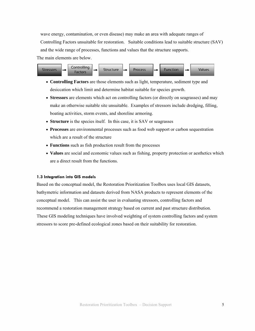
wave energy, contamination, or even disease) may make an area with adequate ranges of

Controlling Factors unsuitable for restoration. Suitable conditions lead to suitable structure (SAV)

and the wide range of processes, functions and values that the structure supports.

The main elements are below.

• Controlling Factors are those elements such as light, temperature, sediment type and

desiccation which limit and determine habitat suitable for species growth.

• Stressors are elements which act on controlling factors (or directly on seagrasses) and may

make an otherwise suitable site unsuitable. Examples of stressors include dredging, filling,

boating activities, storm events, and shoreline armoring.

• Structure is the species itself. In this case, it is SAV or seagrasses

• Processes are environmental processes such as food web support or carbon sequestration

which are a result of the structure

• Functions such as fish production result from the processes

• Values are social and economic values such as fishing, property protection or aesthetics which

are a direct result from the functions.

1.3 Integration into GIS models

Based on the conceptual model, the Restoration Prioritization Toolbox uses local GIS datasets,

bathymetric information and datasets derived from NASA products to represent elements of the

conceptual model. This can assist the user in evaluating stressors, controlling factors and

recommend a restoration management strategy based on current and past structure distribution.

These GIS modeling techniques have involved weighting of system controlling factors and system

stressors to score pre-defined ecological zones based on their suitability for restoration.


6

1.4 Restoration Toolbox Elements

The Restoration Toolbox is comprised of three fundamental elements (Figure 1-1):

(1) Model for Controlling Factors which uses NASA derived datasets with local datasets to

predict areas which are suitable for a species growth.

(2) Benthic Change Tool examines species structure and distribution

(3) Prioritization are scripts which summarize and weight stress and produce final

recommended management actions.

While each can be executed by itself, together they can be used for prioritization of restoration

activities.


Figure 1-1. Restoration Toolbox Elements. Restoration Toolbox Models can be executed by themselves or sequentially for site prioritization and management. Each element analyzes one of the components of the conceptual model and provides feedback to the user based on that component. Finally, salinity for each site is examined to recommend a species appropriate for the site.

7

Controlling Factor Model –Decision Support

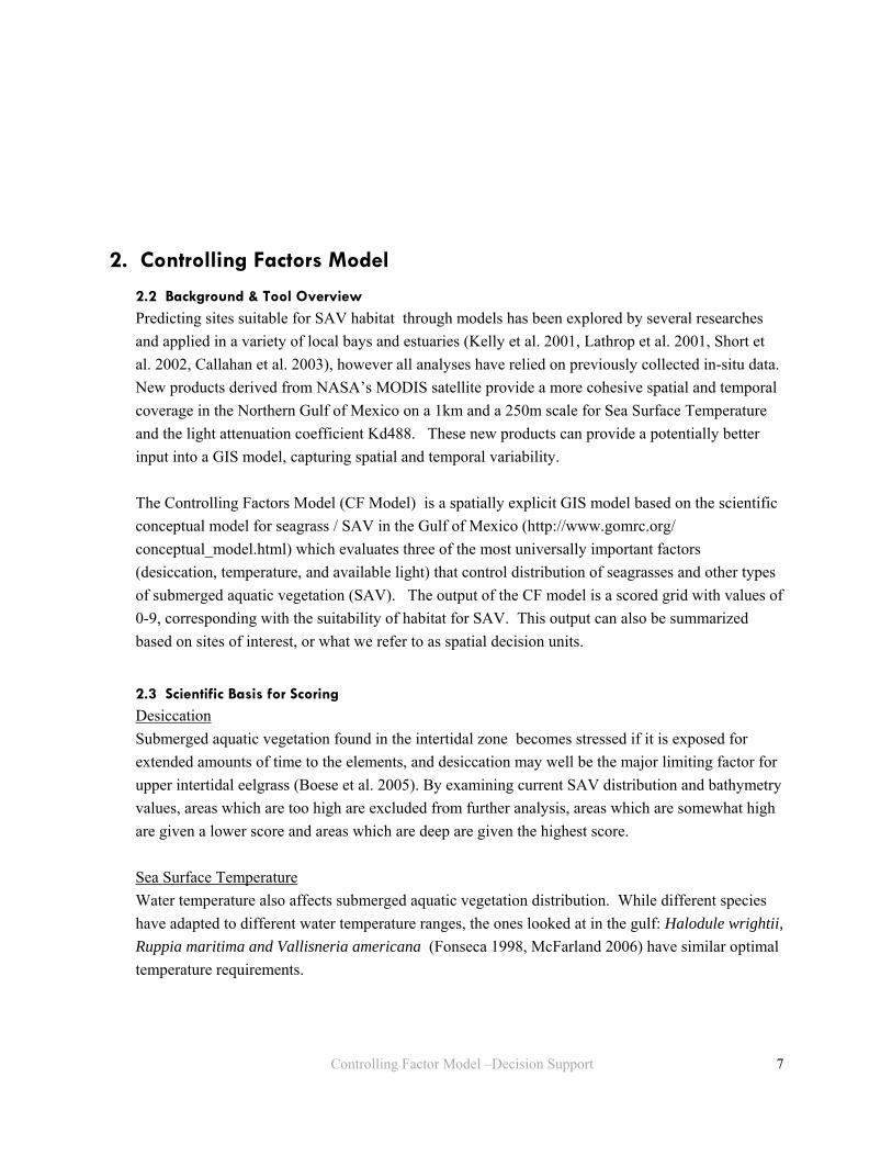
2.2 Background & Tool Overview Predicting sites suitable for SAV habitat through models has been explored by several researches and applied in a variety of local bays and estuaries (Kelly et al. 2001, Lathrop et al. 2001, Short et al. 2002, Callahan et al. 2003), however all analyses have relied on previously collected in-situ data. New products derived from NASA’s MODIS satellite provide a more cohesive spatial and temporal coverage in the Northern Gulf of Mexico on a 1km and a 250m scale for Sea Surface Temperature and the light attenuation coefficient Kd488. These new products can provide a potentially better input into a GIS model, capturing spatial and temporal variability. The Controlling Factors Model (CF Model) is a spatially explicit GIS model based on the scientific conceptual model for seagrass / SAV in the Gulf of Mexico (http://www.gomrc.org/conceptual_model.html) which evaluates three of the most universally important factors (desiccation, temperature, and available light) that control distribution of seagrasses and other types of submerged aquatic vegetation (SAV). The output of the CF model is a scored grid with values of 0-9, corresponding with the suitability of habitat for SAV. This output can also be summarized based on sites of interest, or what we refer to as spatial decision units.

2.3 Scientific Basis for Scoring Desiccation Submerged aquatic vegetation found in the intertidal zone becomes stressed if it is exposed for extended amounts of time to the elements, and desiccation may well be the major limiting factor for upper intertidal eelgrass (Boese et al. 2005). By examining current SAV distribution and bathymetry values, areas which are too high are excluded from further analysis, areas which are somewhat high are given a lower score and areas which are deep are given the highest score. Sea Surface Temperature Water temperature also affects submerged aquatic vegetation distribution. While different species have adapted to different water temperature ranges, the ones looked at in the gulf: Halodule wrightii, Ruppia maritima and Vallisneria americana (Fonseca 1998, McFarland 2006) have similar optimal temperature requirements.

2. Controlling Factors Model

8


Available Light Submerged aquatic vegetation must have sufficient light to carry out photosynthesis. The deeper the plant is, the less light is available, and in fact, the lower edge of vertical distribution is often determined by the amount of light available to plants. This can be described by the following adaptation of Lambert –Beer’s Law where, for any given wavelength: Iλ,z = Iλ ,0 e (-kz) (1)

z is depth Io is irradiance for the wavelength λ at depth 0. K is an attenuation coefficient Iz is irradiance at depth z for wavelength λ.

Using the Kd488 (or the attenuation coefficient at 488nm) product and a separate bathymetry dataset, we can calculate the percent of light at the surface which exists at depth (z). The raster model then extracts values for % surface irradiance (SI) for areas where SAV is currently present and scores areas with suitable light more than those without. Assumptions: This light product assumes that the incoming radiance at the surface of the water is the same throughout the study area. The amount of light present at the water’s surface varies day to day and hour to hour. Weather, time of day, season of year, and solar flares are among the variables that alter the amount of radiance hitting the water’s surface. We assume that the variance of these factors over any particular bay/estuary is negligible for the purposes of this analysis.

9

2.4 Scoring Description of the scoring can be found in Table 2-1. Figure 2-1 provides an illustration of how scores are obtained from distribution characteristics for desiccation and light attenuation. Table 2-1. Scoring regime for Controlling Factors Model. Results for each element are added together, for potential scores ranging from 0-9 for each pixel. Scores 0-6 should be interpreted as unacceptable, 7 marginal, 8 & 9 acceptable for SAV growth.

Controlling Factor Score Score Range

Desiccation 2

1

Excluded

Lowest elevation in bay to + 1σ for distribution + 1σ to maximum elevation for distribution of SAV Areas above maximum elevation for SAV

Sea Surface Temperature 0

1

2

Below 20°C; Above 37°C

20-28°C; 32-37°C

28-32°C

Light attenuation 0

1

2

4

5

Lowest (Iz/Io) in bay to min (Iz/Io) for distribution Minimum (Iz/Io) for distribution to - 1σ for distribution - 1σ for distribution to –1/2 σ for distribution –1/2 σ for distribution to +1/2 σ for distribution +1/2 σ for distribution to Mean Sea Level

Figure 2-1. Scoring for desiccation. Based on cur-rent SAV distribution and bathymetry, we can derive the upper growth limit for SAV. We can then apply that limit to score the entire study area to score areas that are more like the cur-rent habitat higher than those that are not.


10

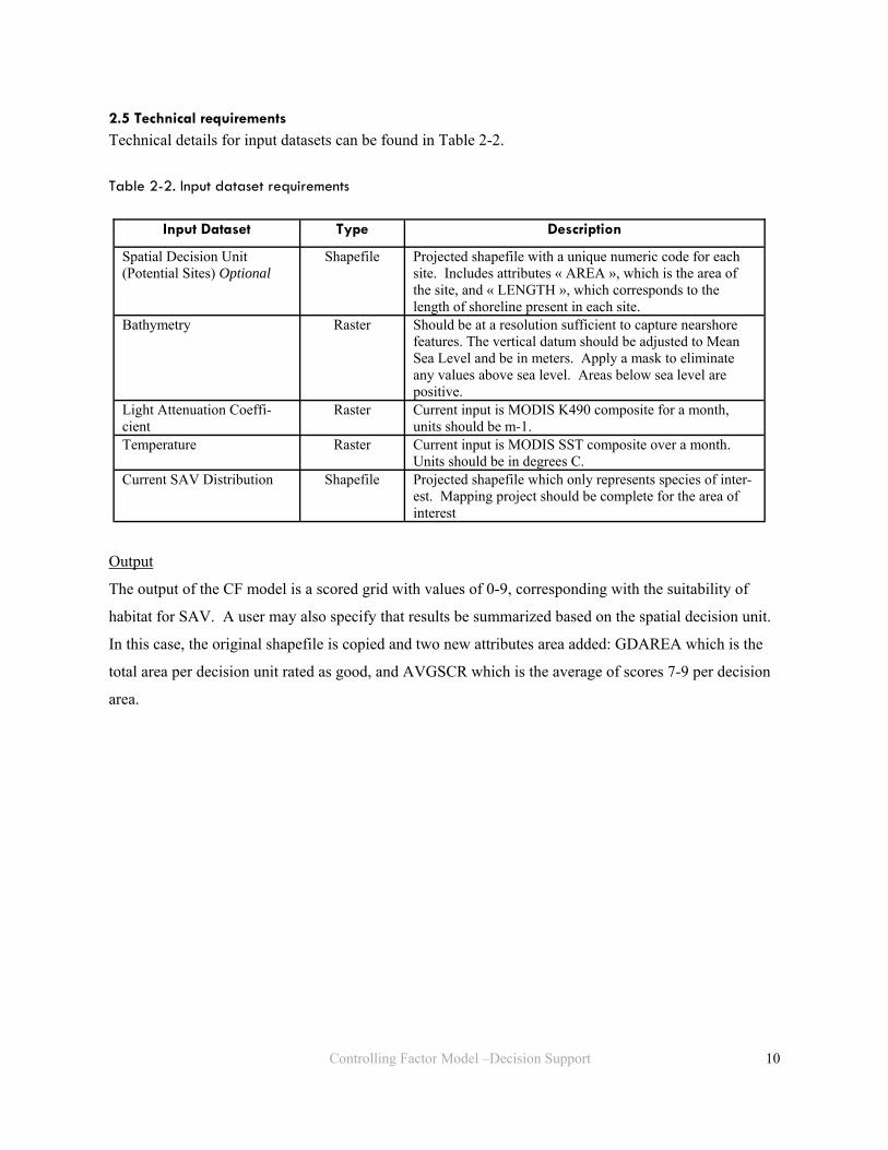
2.5 Technical requirements Technical details for input datasets can be found in Table 2-2. Table 2-2. Input dataset requirements

Output

The output of the CF model is a scored grid with values of 0-9, corresponding with the suitability of

habitat for SAV. A user may also specify that results be summarized based on the spatial decision unit.

In this case, the original shapefile is copied and two new attributes area added: GDAREA which is the

total area per decision unit rated as good, and AVGSCR which is the average of scores 7-9 per decision

area.

Input Dataset Type Description

Spatial Decision Unit (Potential Sites) Optional

Shapefile Projected shapefile with a unique numeric code for each site. Includes attributes « AREA », which is the area of the site, and « LENGTH », which corresponds to the length of shoreline present in each site.

Bathymetry Raster Should be at a resolution sufficient to capture nearshore features. The vertical datum should be adjusted to Mean Sea Level and be in meters. Apply a mask to eliminate any values above sea level. Areas below sea level are positive.

Light Attenuation Coeffi-cient

Raster Current input is MODIS K490 composite for a month, units should be m-1.

Temperature Raster Current input is MODIS SST composite over a month. Units should be in degrees C.

Current SAV Distribution Shapefile Projected shapefile which only represents species of inter-est. Mapping project should be complete for the area of interest


11

Benthic Change Analysis –Decision Support

3. Benthic Change Analysis Tool 3.1 Background & Tool Overview

Over the last century, seagrasses have undergone a dramatic decrease in extent throughout

the Gulf of Mexico (Handley et al. 2006). Though in recent years, the rate of decline has de-

creased and even reversed at some sites, monitoring how and where the extent of SAV changes in

important for resource managers.

The Benthic Change Analysis Tool enables a user to quickly spatially evaluate presence/

absence change for SAV and seagrasses between two time steps. The output of the Benthic

Change Tool is a coded grid with four values.

If the evaluation is carried out as part of the Restoration prioritization assessment the user

also has the option to summarize output raster based on an input shapefile, where each record is

considered a separate ‘Site’ or spatial decision unit. Through this option, three new attributes are

added to the input shapefile: RESTORE, ENHANCE, PRESERVE. The area in each site coded

for each potential management strategy is recorded (see Table 3-1). At this point, these are just

potential management strategies, to be evaluated with other factors.

Table 3-1. Codes for Benthic Change Analysis. Analysis helps select management strategy appro-

priate to site.

3.2 Technical Requirements

Required inputs are summarized in Table 3-2. Both SAV datasets should be projected in

the same coordinate system and in a vector format and representative of only features which are

submerged aquatic vegetation. This analysis only examines change in presence, not changes in

Code Meaning

0 Currently present, historically absent

2 Currently absent, historically absent

4 Currently present, historically present

6 Currently absent, historically present

Potential Management Strategy

Preserve / Conserve

Creation / Enhancement

Preserve / Conserve

Restore

12

density or biomass. Because this tool evaluates change in a raster format, some error will be introduced

in translating vector features to raster features. A cell size should be selected which will capture the vec-

tor data nuances, this is particularly important to ensure that linear fringy SAV is captured. Though this

tool was developed for SAV change analysis, it can be used to evaluate change with any feature be-

tween two time steps.

Table 3-2. Input datasets for Benthic Change Tool. A user may choose to summarize data based on a

spatial decision unit, or may choose just to view the coded raster output.

Input Dataset Type Description Spatial Decision Unit (Potential Sites) Optional



Historical SAV Distribution Shapefile Projected shapefile which only depicts species of interest.

Benthic Change Analysis –Decision Support

13

Stressor Scoring –Decision Support

4. Prioritization Tool 4.1 Background & Tool Overview

The prioritization tool is comprised of 2 scripts which (1) Summarize and standardize stressor

datasets, and (2) Weight and score these datasets and summarizes outputs from prior steps.

The decision unit shapefile is copied and new attributes are added. Final attributes of interest are:

« Salinity », « R_PRIORITY », and « R_ACTION ».

• R_Action lists a potential management strategy per site: Restoration, Conservation,

Enhancement or a combination of the above.

• R_Priority, lists the amount of stress and site suitability.

• Salinity suggests the types of species which would be more suited for the site based on

the salinity level.

What is a spatial decision unit? A spatial decision unit is the minimum unit at which a decision is made. It is at this level that the data is evaluated and summarized for the user. In this case, a spatial decision unit represents a potential res-toration site (see figure to right), and is represented as polygons within a shapefile. Each unit has a unique code, and represents an area with contiguous benthic habitat and geomorphology. The goal is to define units so that a restoration action in the site will affect the function of the entire site.

14

(1) Summarize and standardize stressor datasets

Through the process of summarizing stressor datasets, a user can identify any shapefile which can be

considered stressful to SAV. These stressors are standardized based on the length and area of the site

and recorded in new fields in a Site polygon dataset (Table 4 -1). A summary will also be logged for the

user’s records.

Table 4-1. Summarizing stressor datasets per spatial decision unit. Datasets must have line, point, or

polygon geometries to be used.

(2) Weight and score datasets

At this stage, the user selects identifies a relative weighting for each stressor.

First, each factor is scored between 1-5 based on the severity of the standardized stressor in the polygon.

Scoring is by quintile and relative to other scores in the area. Decision units with no stressor present

receive a score of zero. This relative ranking is then multiplied by the user defined weight. After

calculating the relative stress, the stressor scores are totaled for each spatial decision unit.

Finally, each site with some type of stress is ranked 1-3 based on the amount of relative stress

based on their scores. 1 - Low, 2 - Medium, and 3 - High.

Salinity

High and low seasonal averages for salinity are extracted for each site and compared against the

salinity ranges for each species. The species which is most adequate for the site is recorded as in Table

4-2.

Input Stressor Dataset Type

Function Output Example of stressor

Line For each decision unit polygon, % total shoreline covered by linear feature will be recorded

Shoreline armoring

Point For each decision unit polygon, tool will record: • Number of data points present • Standardized to number of points per

1000 ft / m

Boat launches Piers

Marinas Outfalls

Polygon • For each decision unit polygon, % of total area in unit covered by new poly-gon feature is recorded

Invasive species Landslides

New attribute in deci-sion unit shapefile with calculations. Attribute name will be the first seven characters of the file name with an exten-sion of sd for a point dataset, and pc for a line or polygon data-set.


15

Salinity Category High value (psu) Low value (psu)

Seagrass >24 >14

Freshwater SAV < 6 —

Oligohaline Ruppia 6-15 —

Ruppia & Halodule possible, outside optimal range

16-24

< 14

Table 4-2. SAV species category by salinity. Salinity category is recorded under new attribute

“Salinity” for each potential site within decision unit shapefile.

Restoration Management Strategy

The restoration management strategy uses results from the benthic change tool to evaluate what structure

is present now and how it has changed over time to recommend a potential management strategy, under

the new attribute R_Action. In addition, the tool evaluates the total area per site with suitable habitat to

discern whether the conditions are adequate for restoration. Table 4-3 provides a summary.

Table 4-3. Potential Management Action. Management actions are based on the results of prior analysis and the attributes that they recorded in the decision unit file. RESTORE is the total area per site where SAV was present historically, but absent present day. PROTECT is the total area per site where SAV is currently present. GD_AREA is the total area per site with adequate controlling factors.

Attributes within decision unit shapefile RESTORE PROTECT GD_AREA

Restore > 5 ha <1 ha > 5ha

Protect & Restore > 5ha >1ha > 5ha

Protect <5 ha >1ha > 1ha

Enhance <5ha <1ha —

Potential Restoration Action


16

Restoration Category At this stage, the controlling factor scores are also ranked 1,2, or 3 depending on the average of accept-

able scores (7-9) per site. Equal numbers of sites are placed in each group. Sites with no acceptable

scores are ranked 0. These rankings are combined with the stressor score, for the final restoration cate-

gory R_Priority. Table 4-4 summarizes how categories are defined.

Table 4-4. Restoration Priority Definitions. Restoration priorities summarizes the scores from the Control-

ling Factors and Stressors Analysis.

4.2 Interpreting Results The three attributes: Salinity, R_Priority, and R_Action must be viewed together to evaluate potential

management actions. A site with low controlling factors, for example, probably would not make a good

site for restoration of SAV. Managers might be interested in changing the controlling factors, and in

many cases this would be related to characteristics of the watershed. On the other hand, a site with High

Controlling Factors and Low or Medium Stress with a restoration action of RESTORE, might be an

ideal site to replant SAV. In a site with High Stress, High CF and a Protect action, managers may want

to try to reduce stress to protect the current SAV population.

It is also important to keep in mind that the quality of results depend on the integrity and quality of the

input datasets. If there are errors in the input datasets, there will be errors in the results as well.

This analysis should be viewed as a preliminary step in selecting a restoration management action ap-

propriate for an area. It is equally important to visit the site in person for a better understanding of the

ecological characteristics.

R_Priority Category Controlling Factor Score

Stressor Score

Low Controlling Factors (CF) 0—1 Any

High Stress, Medium CF 2 3

Med Stress, Medium CF 2 2 Low Stress, Medium CF 2 1

High Stress, High CF 3 3

Med Stress, High CF 3 2 Low Stress, High CF 3 1


17

4.3 Technical Requirements

Spatial decision unit dataset:

• Unique ID The site dataset must be made up of polygons, with everything that is considered

a site having a unique ID to identify it.

• LENGTH The site dataset must have an attribute LENGTH which represents the length of

shoreline present

• AREA The site dataset must also have an attribute AREA which represents the total area of

each site

• Projection—The dataset should be projected with a linear unit of meters. The projection

should be the same for all input stressor datasets

Stressor datasets

• Only feature of interest should exit in dataset

• Dataset should be projected in the same projection as the site dataset

• Datasets should be shapefiles with only points, lines or polygons represented


18

5. Case Study - Mobile Bay, AL 5.1 Background on Mobile Bay

Mobile Bay is one of the many estuaries and bays located within

the Gulf of Mexico, and it has a very dynamic system (Figure 5 –

1). On the north end of the bay, freshwater influx is high, and in

the south, high salinity from the ocean dominates. The metro-

politan area of Mobile, AL is located on the northwest edge, and

smaller towns and community dot the shoreline.

Conversion of forest to farmland and development of rural and

coastal areas are common development activities. Within the bay

itself, dredging, vessel activity, shoreline armoring and shoreline

structures put additional stress on the nearshore habitat. Hurri-

canes and tropical storms add stress as well. Recently, invasive

aquatic vegetation has been found in Mobile Bay.

Case Study –Decision Support

Where have all the seagrasses gone? Interpretation of early aerial photos from 1940-1966 allowed for SAV to be mapped in portions of Mobile Bay. Recent aerial photos show a diminished distribution of SAV. The figure to the right shows where the most re-cent mapping effort identified SAV compared with map-ping from historical photos. There are many suggested theories why this loss is seen. Some scientists point to altered salinity regimes within the bay, others to development and nearshore stresses, and others still to increased turbidity. For further details about this study, please see: Vittor & Associates. 2005. Historical SAV Distribution in the Mobile Bay National Estuary Program Area and Ranking Analy-sis of Potential SAV Restoration Sites. Prepared for Mobile Bay National Estuary Program, Mobile, AL. p 17.

Figure 5-1. Mobile Bay, AL.

19

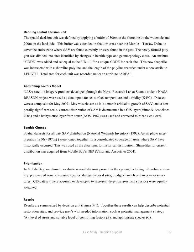
Defining spatial decision unit

The spatial decision unit was defined by applying a buffer of 500m to the shoreline on the waterside and

200m on the land side. This buffer was extended in shallow areas near the Mobile—Tensaw Delta, to

cover the entire zone where SAV are found currently or were found in the past. The newly formed poly-

gon was divided into sites identified by changes in benthic type and geomorphology class. An attribute

“CODE” was added and set equal to the FID +1, for a unique CODE for each site. This new shapefile

was intersected with a shoreline polyline, and the length of the polyline recorded under a new attribute

LENGTH. Total area for each unit was recorded under an attribute “AREA”.

Controlling Factors Model

NASA satellite imagery products developed through the Naval Research Lab at Stennis under a NASA

REASON project were used as data inputs for sea surface temperature and turbidity (K490). Datasets

were a composite for May 2007. May was chosen as it is a month critical to growth of SAV, and a tem-

porally significant scale. Current distribution of SAV is documented in a GIS layer (Vittor & Associates

2004) and a bathymetric layer from sonar (NOS, 1962) was used and corrected to Mean Sea Level.

Benthic Change

Spatial datasets for all past SAV distribution (National Wetlands Inventory (1992), Aerial photo inter-

pretation 1950s -1970s) ) were joined together for a consolidated coverage of areas where SAV have

historically occurred. This was used as the data input for historical distribution. Shapefiles for current

distribution was acquired from Mobile Bay’s NEP (Vittor and Associates 2004).

Prioritization

In Mobile Bay, we chose to evaluate several stressors present in the system, including: shoreline armor-

ing, presence of aquatic invasive species, dredge disposal sites, dredge channels and overwater struc-

tures. GIS datasets were acquired or developed to represent these stressors, and stressors were equally

weighted.

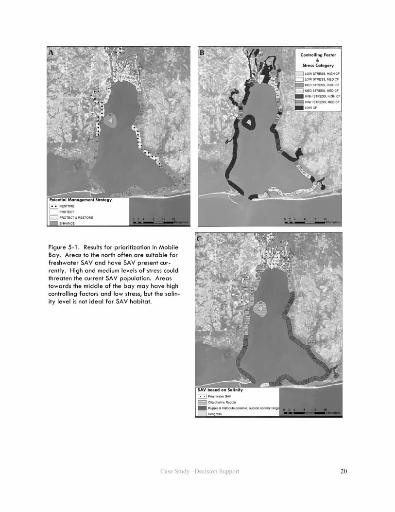
Results

Results are summarized by decision unit (Figure 5-1). Together these results can help describe potential

restoration sites, and provide user’s with needed information, such as potential management strategy

(A), level of stress and suitable level of controlling factors (B), and appropriate species (C).


20


Figure 5-1. Results for prioritization in Mobile Bay. Areas to the north often are suitable for freshwater SAV and have SAV present cur-rently. High and medium levels of stress could threaten the current SAV population. Areas towards the middle of the bay may have high controlling factors and low stress, but the salin-ity level is not ideal for SAV habitat.

A B

C

21

6. References Boese, B. L. B. D. Robbins and G. Thursby. 2005. Desiccation is a limiting factor for eelgrass

(Zostera marina L.) distribution in the intertidal zone of a northeastern Pacific (USA) estu-ary. Botanica Marina 48: 274-83.

Callahan, A., R. McGuinn, and J. Marshall. Lake St. Clair Integrated Coastal Management (ICM) Tool: Draft Software Development Plan, Perot Systems, 2003.

Fonseca, M. S. Kenworthy W. J. Thayer G. T. Guidelines for Conservation and Resotration of Sea-grasses in the Unites States and Adjacent Waters, NOAA Coastal Occean Decision Analysis Series, No. 12. NOAA Coastal Ocean Office, Silver Springs, MD, 1998.

Handley, L., Altsman, D., and DeMay, R., eds., 2007, Seagrass Status and Trends in the Northern Gulf of Mexico: 1940-2002: U.S. Geological Survey Scientific Investigations Report 2006-5287 and U.S. Environmental Protection Agency 855-R-04-003, p267.

Kelly, N., M. Fonseca, and P. Whitfield. "Predictive Mapping for Management and Conservation of

Seagrass Beds in North Carolina." Aquatic Conservation: Marine and Freshwater Ecosys-tems 11: 437-51.

Lathrop, R., R. Styles, S. Seitzinger, and J. Bognar. "Use of GIS Mapping and Modeling Approaches to Examine the Spatial Distribution of Seagrasses in Barnegat Bay, New Jersey." Estuaries 24, no. 6A (2001): 904-16.

McFarland, D. G. Reproductive Ecology of Vallisneria Americana Michaux, ERDC/TN SAV-06-4. US Army Corps of Engineers, Engineer Research and Development Center, 2006.

Short, F., B. Davis, C. Kopp, C. Short, and D. Burdick. 2002. "Site-Selection Model for Optimal Transplantation of Eelgrass Zostera Marina in the Northeaster US." Marine Ecology Pro-gress Series 227: 253-67.

Vittor and Associates. 2004. Mapping of Submerged Aquatic Vegetation in Mobile Bay and Adjacent Waters of Coastal Alabama in 2002. Prepared for Mobile Bay National Estuary Program. Mobile Bay, AL. p 63.

Vittor & Associates. 2005. Historical SAV Distribution in the Mobile Bay National Estuary Program Area and Ranking Analysis of Potential SAV Restoration Sites. Prepared for Mobile Bay National Estuary Program, Mobile. AL. p 17.

22

Appendix A– Overview of User’s Tools and Guide Which version of the tools should I use? The restoration toolsets are available in two forms:

• Conceptual Model Explorer (CME) on the web • ArcGIS Toolboxes (Controlling Factors and Benthic Change only)

Conceptual Model Explorer The tool within the CME has more parameters hardwired than the ArcGIS toolbox but allows com-plete execution of the Restoration Toolbox elements. This may be ideal for users with limited ex-perience with GIS, or no access to ArcGIS, or those interested specifically in Mobile Bay. ArcGIS Toolbox The Restoration Toolbox should be used for those with access to ArcGIS 9.2, with Spatial Analyst. The toolbox does not contain the prioritization tool, but does allows users to examine habitat suit-ability for SAV (Controlling Factors) and to evaluate change per polygon between two timesteps (Benthic Change). Complete instructions are housed within the tool itself.

How do I access and install these different versions? Conceptual Model Explorer

This web based tool provides a simple user interface and requires no downloading of tools or data. However, at present time, it is configured for execution only for Mobile Bay, AL with limited sub-stitution capability. To access the tool, go to (http://persephone.bioe.orst.edu/cme/) and follow user’s guide.

Instructions for installation of Restoration Toolbox

Requirements: Toolboxes are formatted to be executed in ArcInfo 9.2 with a current Spatial Analyst extension. Instructions:

1) Download zipped toolbox folder to your computer and extract contents to a folder 2) Open ArcMap 3) Right click on the top level “ArcToolbox” within your ArcToolbox window, and select

“Add Toolbox” 4) Navigate to the place on your computer where you saved the folder and select the toolbox. 5) The toolbox should now appear within the ArcToolbox window.

To execute, simply follow directions within tool.

23

Appendix B: User’s Guide: Restoration Toolbox within the Conceptual Model Explorer Background The Restoration Prioritization Toolbox forms part of an integrated system within the Gulf of Mexico Regional Collaborative’s (GOMRC) framework to help decision makers from a variety of agencies in their environmental restoration planning process, focusing in this case on submerged aquatic vegetation. GOMRC’s approach to prioritizing sites for restoration is based on a science- based representation of how the system functions, known as an ecological conceptual model. A conceptual model was developed for SAV habitat to help users understand how ecosystem stressors and certain coastal habitat conditions, referred to as controlling factors, can influence SAV distribution and abundance. Geospatial data can provide insights on various elements of the conceptual model for SAV habitat. Analysis of this data enables use to predict where:

1) Controlling factor ranges are suitable for maintaining healthy SAV 2) SAV distribution has changed over time, and 3) Local stressors are influencing SAV habitat

GoMRC’s Restoration Toolbox provides a means of collectively evaluating controlling factors, SAV distribution and local stresses, and recommending sites for SAV restoration in Mobile Bay. Conceptual Model Explorer (CME) provides a simple user interface to execute complex spatial analyses and provide results. For those familiar with ArcGIS products, the restoration toolbox runs analyses on ESRI’s ArcServer through the CME, and a user can execute with default datasets, provide new datasets, change weighting and choose to view or download results. Restoration Toolbox Elements The Restoration toolset contains three fundamental models that will run sequentially:

(1) Model for Controlling Factors which uses NASA derived datasets with local datasets to predict areas which are suitable for a species growth.

(2) Benthic Change Tool examines species structure and distribution (3) Prioritization are scripts which summarize and weight stress and produce final

recommended management actions. Further details about each of these models is available on-line at www.gomrc.org.

24

Restoration Toolbox Execution - Four steps The restoration framework can be executed by following four simple steps:

1. Log on to the conceptual model explorer

2. Select “Execute Workspace”

3. Configure set-up if desired

4. Download or map results

1. Log on to the conceptual model explorer (http://persephone.bioe.orst.edu/cme/)

While a casual user may view conceptual models and tools without logging on, a log in is

required to execute or change tools. Users can easily sign up for a free user account, by selecting

Create New User from log in screen.

After logging on, the user will have a choice of different tools and models to view, edit or

execute within the CME. In this case, we will select the link “SAV Restoration Prioritization

Tool”. The toolbox workspace (as shown below) will appear. This is a visual representation of

analysis elements. The toolbox is comprised of three separate models that will run sequentially.

Input datasets are grouped by the category of the scientific conceptual model they represent:

Controlling Factors, Stressors or Structure.

25

Models are visually represented by orange diamonds, and in this case are referred to as “Adapters”.

Input datasets are shown in blue, and outputs in yellow. In this case the shapefile for restoration sites is shown in green. After execution, newly derived datasets may either be visualized in our interactive map, or downloaded. Relationships are represented by blue arrows. They can represent inputs to a model and outputs from a model. Further details on these components and the CME itself are available through the CME help

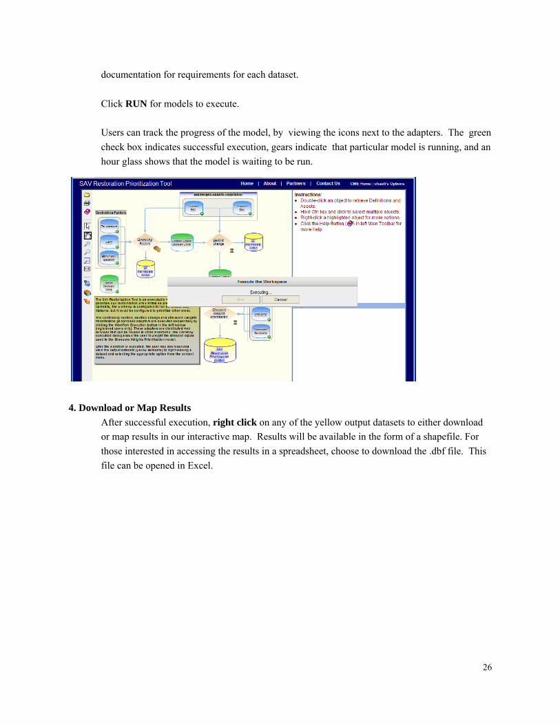
2. Select “Execute the Workspace”

To execute the spatial analysis, users should click on the “Execute Workspace” button on the left side toolbar. This will launch a user interface to change input datasets or weights. The window below will pop up.

3. Configure set-up if desired The window allows access to change default inputs for (a) Scoring of stressors or (b) Input datasets (Experimental).

(a) Scoring of Stressors Click on the pencil. The “Edit Parameter” dialog box will appear. Users can change the relative importance of each unique stressor by entering a new number (integers ) in the Weight box. After changes, user should select “Save”. (b) Input datasets (Experimental) Input datasets can also be changed by clicking on the pencil. If access to the entire dataset is available online, the user can enter the URL. If the user has the dataset locally on their computer, they can upload the file (as long as it is under 10MB). Please see entire

26

documentation for requirements for each dataset. Click RUN for models to execute. Users can track the progress of the model, by viewing the icons next to the adapters. The green check box indicates successful execution, gears indicate that particular model is running, and an hour glass shows that the model is waiting to be run.

4. Download or Map Results

After successful execution, right click on any of the yellow output datasets to either download or map results in our interactive map. Results will be available in the form of a shapefile. For those interested in accessing the results in a spreadsheet, choose to download the .dbf file. This file can be opened in Excel.

27

Appendix C. Technical documentation of Restoration Prioritization Toolbox Background

With the growing population and pressure to develop coastal areas as well as coastal watersheds, conserva-

tion and restoration of coastal ecosystems is a high priority for the nation. Managers must make decisions on com-

plex problems every day, and having a credible scientific basis for these decisions is critical. In addition, they need

to plan and implement restoration in cost effective ways in order to maximize results for the money spent.

Among the most often sought after tool by managers is one that prioritizes restoration projects. A prioritiza-

tion decision tool provides one of the bases for making investments in restoration projects. Ideally the tool con-

tains the relevant scientific underpinnings, and facilitates the decision making process by providing an effective

interactive mechanism.

The Restoration Prioritization Toolbox forms part of an integrated system within the Gulf of Mexico Re-

gional Collaborative (GoMRC) framework to facilitate decisions related coastal ecosystem restoration, specifically

the management of submerged aquatic vegetation. Based on the conceptual model, the Restoration Prioritization

Toolbox uses local GIS datasets, bathymetric information and datasets derived from NASA products to represent

elements of the conceptual model. This can assist the user in evaluating stressors, controlling factors and recom-

mend a restoration management strategy based on current and past structure distribution. These GIS modeling

techniques have involved weighting of system controlling factors and system stressors to score pre-defined eco-

logical zones based on their suitability for restoration.

Application Description

The toolbox is comprised of three elements:

1. Model for Controlling Factors which uses NASA derived datasets with local datasets to

predict areas which are suitable for a species growth.

2. Benthic Change Tool examines species structure and distribution

3. Prioritization are scripts which summarize and weight stress and produce final recom-

mended management actions.

The Controlling Factors and Benthic Change tools are available both within the Conceptual Model Ex-

plorer (CME) and as stand alone ArcGIS toolboxes. The prioritization scripts are only executable

through the CME.

Each tool was originally written in Python for execution in ArcInfo 9.2 with Spatial Analyst license and

accessed by an ArcGIS toolbox. Scripts were recoded for execution within ArcServer.

28

Expected inputs for each model and outputs can be summarized in the tables below.

Input Dataset Type Description

Spatial Decision Unit (Potential Sites)


Bathymetry Raster Should be at a resolution sufficient to capture nearshore (30m pixels). The vertical datum should be adjusted to Mean Sea Level and be in meters. Apply a mask to elimi-nate any values above sea level. Areas below sea level are positive.

Light Attenuation Coeffi-cient

Raster Current input is MODIS K490 composite for a month, units should be m-1.

Temperature Raster Current input is MODIS SST composite over a month. Units should be in C


Historical SAV Distribution Shapefile Projected shapefile which only depicts species of interest.

Salinity Shapefile Projected shapefile with High and Low salinity values recorded.

Stressor Datasets Shapefiles Projected shapefiles which represent environmental stress-ors of interest which occur within the spatial decision unit.

29

Processing Detailed information on data processing and scoring is available Restoration Prioritization Toolbox : Documenta-tion and User’s Guides 2007 QA, Validation and Testing The desktop toolbox went through a functional QA process as well as a critical scientific peer review of modeling and prioritization methods.

Relationship to other GoMRC Tools

The prioritization scheme is based on the Scientific Conceptual Model for SAV Restoration: http://www.gomrc.org/conceptual_model.html The models are currently embedded in the Conceptual Model Explorer:

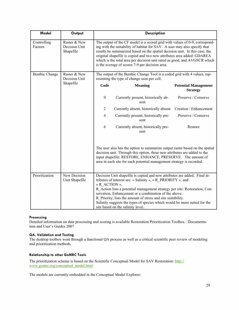
Model Output Description

Controlling Factors

Raster & New Decision Unit Shapefile

The output of the CF model is a scored grid with values of 0-9, correspond-ing with the suitability of habitat for SAV. A user may also specify that results be summarized based on the spatial decision unit. In this case, the original shapefile is copied and two new attributes area added: GDAREA which is the total area per decision unit rated as good, and AVGSCR which is the average of scores 7-9 per decision area.

Benthic Change Raster & New Decision Unit Shapefile

The output of the Benthic Change Tool is a coded grid with 4 values, rep-resenting the type of change seen per cell.

The user also has the option to summarize output raster based on the spatial decision unit. Through this option, three new attributes are added to the input shapefile: RESTORE, ENHANCE, PRESERVE. The amount of area in each site for each potential management strategy is recorded.

Code Meaning Potential Management Strategy

0 Currently present, historically ab-sent

Preserve / Conserve

2 Currently absent, historically absent Creation / Enhancement

4 Currently present, historically pre-sent

Preserve / Conserve

6 Currently absent, historically pre-sent

Restore

Prioritization New Decision Unit Shapefile

Decision Unit shapefile is copied and new attributes are added. Final at-tributes of interest are: « Salinity », « R_PRIORITY », and « R_ACTION ». R_Action lists a potential management strategy per site: Restoration, Con-servation, Enhancement or a combination of the above. R_Priority, lists the amount of stress and site suitability. Salinity suggests the types of species which would be more suited for the site based on the salinity level.

Date post:	14-May-2018
Category:	Documents
Upload:	lytuong
View:	237 times
Download:	0 times

Restoration Prioritization Toolset: Documentation … Restoration Prioritization Toolset:...

Documents