23 11 Article 13.1.3 Journal of Integer Sequences, Vol. 16 (2013), 2 3 6 1 47 Restricted Weighted Integer Compositions and Extended Binomial Coefficients Steffen Eger School of Computer Science Carnegie Mellon University Pittsburgh, PA 15213 USA [email protected]Abstract We prove a simple relationship between extended binomial coefficients — natural extensions of the well-known binomial coefficients — and weighted restricted integer compositions. Moreover, we give a very useful interpretation of extended binomial coef- ficients as representing distributions of sums of independent discrete random variables. We apply our results, e.g., to determine the distribution of the sum of k logarithmi- cally distributed random variables, and to determining the distribution, specifying all moments, of the random variable whose values are part-products of random restricted integer compositions. Based on our findings and using the central limit theorem, we also give generalized Stirling formulae for central extended binomial coefficients. We enlarge the list of known properties of extended binomial coefficients. 1 Introduction An integer composition of a nonnegative integer n with k summands, or parts, is a way of writing n as a sum of k nonnegative integers, where the order of parts is significant. We call the integer composition S -restricted if all parts lie within a subset S of the nonnegative integers. Compositions with (various types of) restrictions on part sizes have recently been studied in, e.g., [11, 12, 24, 25, 32] and for probabilistic results on such compositions see [4, 6, 7, 8, 27, 33, 35]. A classical result in combinatorics is then that the number of S - restricted integer compositions of n with k parts is given by the coefficient of x n of the polynomial or power series (see, e.g., [24]) ( s∈S x s ) k . 1
Transcript
23 11
Article 13.1.3Journal of Integer Sequences, Vol. 16 (2013),2
3
6
1
47
Restricted Weighted Integer Compositions
and Extended Binomial Coefficients
Steffen EgerSchool of Computer ScienceCarnegie Mellon University
We prove a simple relationship between extended binomial coefficients — naturalextensions of the well-known binomial coefficients — and weighted restricted integercompositions. Moreover, we give a very useful interpretation of extended binomial coef-ficients as representing distributions of sums of independent discrete random variables.We apply our results, e.g., to determine the distribution of the sum of k logarithmi-cally distributed random variables, and to determining the distribution, specifying allmoments, of the random variable whose values are part-products of random restrictedinteger compositions. Based on our findings and using the central limit theorem, wealso give generalized Stirling formulae for central extended binomial coefficients. Weenlarge the list of known properties of extended binomial coefficients.
1 Introduction
An integer composition of a nonnegative integer n with k summands, or parts, is a way ofwriting n as a sum of k nonnegative integers, where the order of parts is significant. Wecall the integer composition S-restricted if all parts lie within a subset S of the nonnegativeintegers. Compositions with (various types of) restrictions on part sizes have recently beenstudied in, e.g., [11, 12, 24, 25, 32] and for probabilistic results on such compositions see[4, 6, 7, 8, 27, 33, 35]. A classical result in combinatorics is then that the number of S-restricted integer compositions of n with k parts is given by the coefficient of xn of thepolynomial or power series (see, e.g., [24])
These coefficients, in turn, which generalize the ordinary binomial coefficients, and areusually called polynomial coefficients or extended binomial coefficients, exhibit fascinatingmathematical properties, closely resembling those of binomial coefficients. Although theyappeared explicitly as far back as De Moivre’s The Doctrine of Chances [14] in 1756, theirsystematic study has apparently only recently been investigated (cf. [17]). In the present pa-per, we give a complete characterization of extended binomial coefficients, over commutativerings R, in terms of sums, over restricted integer compositions, of part-products of integercompositions, where each part is mapped, via a function f , to a value in the ring (Theorem1). It is a straightforward exercise to show that these sums, when f is integer-valued, countcolored monotone lattice paths or, simply, colored integer compositions (third proof of The-orem 1 and Remark 4). Colored integer compositions, in turn, have recently been studied(cf. [1, 23, 28, 29]), for example, in the situation when part s ∈ S comes in s different colors(‘n-colored compositions ’) and, simultaneously with, but independently of the present paper,when part s ∈ S may take on cs ∈ C different colors [34] (‘C-colored compositions ’), wherecs is a nonnegative integer. We term the generalization of these two concepts considered inthe present work analogously f -weighted compositions, and, under restrictions on part sizes,S-restricted f -weighted compositions.
We give three proofs of the named simple result, Theorem 1, each shedding new light onthe problem. Our first proof is a direct rewriting of extended binomial coefficients in termsof integer partitions, using commutativity of R and the multinomial theorem. Our secondproof, which yields a very useful characterization of extended binomial coefficients as givingthe distribution of the sum of k independent multinomials, generalizes De Moivre’s originalobservation that extended binomial coefficients arise as the distribution of the sum of kindependent random variables, distributed uniformly on the set {0, 1, . . . , l} for some l > 0;our proof is inspired, too, by [3] and [9], who discuss related settings. Our third proof may beconsidered a direct application of our second proof due to the well-known characterizationof sums of independent discrete random variables, i.e., random walks, as directed latticepaths, but we give an independent proof that uses the Vandermonde property (Lemma 2) ofextended binomial coefficients.
After having proven our main theorem, we specify, in Section 6, a variety of applications ofour main result, which indicate the generality of our approach. We structure our applicationsin three parts:
• Firstly, we discuss S-restricted f -weighted integer compositions for particular choicesof S and f , as have been considered in the literature. For example, we consider thecase where S is the finite set {0, 1, . . . , l}; where S = N\{s0} [12], the nonnegativeintegers without a particular element s0; the cases when f(s) = s, which yields, asmentioned, n-colored compositions; when f(s) = sr, which allows the derivation ofmoments of random integer compositions [33, 35]; and a few other cases, such as whenf is complex-valued or takes values in the power set of a set S. In all these situations,our main theorem allows us to effortlessly derive a closed-form solution (and associatedidentities and properties) for the combinatorial object we consider, the total weight ofall S-restricted integer compositions of n with k parts under the weighting function f ,in terms of extended binomial coefficients.
2
• Secondly, we present the most important application of our main result, as we feel,namely, the situation when f is a discrete probability measure. In this case, ourmain theorem allows us to derive a closed-form formula for the distribution of thesum of k independent random variables, which we use, e.g., to specify a novel closed-form formula for the sum of k logarithmically distributed random variables. In thesame context, we are able to derive generalized Stirling formulae for central extendedbinomial coefficients, by equating the exact closed-form solution with the asymptoticdistribution, as implied by the central limit theorem. We also show, and make use ofthe fact, that extended binomial coefficient identities admit intriguing and convenientprobabilistic proofs.
• Finally, we derive a few combinatorial proofs of extended binomial coefficient identities,based on their interpretation as representing (the total weight of all) S-restricted f -weighted integer compositions.
2 Notation and preliminaries
By Z we denote the set of integers, by N we denote the set of nonnegative integers and by P
we denote the set of positive integers. Then, an integer composition of a nonnegative integern ∈ N is a tuple π = (π1, . . . , πk) ∈ N
k, k ∈ N, of nonnegative integers such that
n = π1 + · · ·+ πk,
where the πi are called parts. We call an integer composition of n S-restricted (cf. [27]) fora finite subset S of N if all parts satisfy πi ∈ S. We denote the set of S-restricted integercompositions by CS(n, k) and by cS(n, k) we denote its size, cS(n, k) =
∣
∣CS(n, k)∣
∣.Furthermore, we call a tuple of nonnegative integers (λ1, . . . , λk) ∈ N
k where λ1 ≥ λ2 ≥· · · ≥ λk an integer partition of n (‘unordered composition’) and analogously denote byPS(n, k) the set of S-restricted integer partitions and by pS(n, k) its size. Obviously, each S-restricted integer partition λ = (λ1, . . . , λk) may be uniquely represented by a tuple (αs)s∈S— αs, αs ∈ N, denoting the multiplicity of s ∈ S in λ — where
∑
s∈S αs = k and∑
s∈S sαs =n. We silently identify the two representations.
Next, let R = (R,+, ·,0,1) be a commutative ring with addition +, multiplication · andadditive and multiplicative identities 0 and 1, respectively. Let f be a function f : S → R.In the current work, our interest lies, in particular, in the quantity
dS,f (n, k) =∑
π=(π1,...,πk)∈CS(n,k)f(π1) · · · f(πk), (1)
where, obviously, the summation symbol refers to the addition operation + inR, and likewisefor multiplication ·.
We also remind the reader of the multinomial theorem. For m ∈ N, x1, . . . , xm ∈ R, andk ∈ N as above,
(x1 + · · ·+ xm)k =
∑
α1≥0,...,αm≥0
α1+···+αm=k
(
k
α1, . . . , αm
)
xα11 · · · xαm
m , (2)
3
where(
kα1,...,αm
)
are the respective multinomial coefficients [3], which, for αs ∈ N, s ∈ S, and
k =∑
s∈S αs, denote the number of arrangements of k objects of∣
∣S∣
∣ different types — αs oftype s for s ∈ S — in a sequence of length k.
Finally, for S, k, and n as above, we denote the coefficient, called polynomial coefficientor extended binomial coefficient in the literature (cf. [3, 9, 13, 17]), of xn in the expansion ofthe univariate polynomial (
∑
s∈S f(s)xs)k ∈ R[x] as
(
kn
)
(f(s))s∈S. More precisely, we let
(
k
n
)
(f(s))s∈S
= [xn](∑
s∈Sf(s)xs)k (3)
where we use the standard notation [xn]h(x) to denote the coefficient of xn of the polynomialh(x) =
∑
i aixi, i.e., [xn]h(x) = an.
3 Main theorem
Theorem 1. With notation as in Section 2,
dS,f (n, k) =
(
k
n
)
(f(s))s∈S
.
4 Proofs of the main theorem
Proof of Theorem 1, 1. Rewriting (1) in terms of partitions, we find that dS,f allows thefollowing representation, because of commutativity of multiplication in R and the combina-torial interpretation of multinomial coefficients as above,
dS,f (n, k) =∑
(αs)s∈S∈PS(n,k)
(
k
(αs)s∈S
)
∏
s∈Sf(s)αs =
∑
αs≥0∑
s αs=k∑s sαs=n
(
k
(αs)s∈S
)
∏
s∈Sf(s)αs . (4)
On the other hand, substituting xs = f(s)xs, s ∈ S, in the multinomial theorem (2), we findthat
(
∑
s∈Sf(s)xs
)k
=∑
αs≥0∑s αs=k
(
k
(αs)s∈S
)
(
∏
s∈Sf(s)αs
)
x∑
s sαs . (5)
Thus,
(
k
n
)
(f(s))s∈S
= [xn](
∑
s∈Sf(s)xs
)k
= dS,f (n, k)
as required.
4
For our next proof, we assume that R is the field of real numbers, that f(s) ≥ 0 for alls ∈ S and that
∑
s∈S f(s) 6= 0. We also make use of the following observation. If
X1 + · · ·+Xk = n,
where X1, . . . , Xk are S-valued random variables, then the Xj variables form an S-restrictedinteger composition of the integer n with k parts. Thus, by mutual disjointness of any twodistinct ‘composition events’ and additivity of probability measures,
Proof of Theorem 1, 2. Let Xi, i = 1, . . . , k, be identically and independently distributedrandom variables, where each Xi is multinomially distributed on the set S, where the prob-ability that Xi takes on the value s ∈ S is p(s) = f(s)∑
s′∈S f(s′). We derive the distribution of
the sum X1 + · · · +Xk in two ways, first by considering its probability generating function(pgf) and then by a combinatorial argument using (6).
Consider the pgf GXi(x) =
∑∞n=0 p(n)x
n of Xi. Because X1, . . . , Xk are independent, wehave by elementary facts about pgf’s that
GX1+···+Xk(x) = GX1(x) · · ·GXk
(x) =(
∑
s∈Sp(s)xs
)k
=∑
n≥0
(
k
n
)
(p(s))s∈S
xn.
Therefore,
P [X1 + · · ·+Xk = n] =G
(n)X1+···+Xk
(0)
n!=
n!
n!
(
k
n
)
(p(s))s∈S
=
(
k
n
)
(p(s))s∈S
, (7)
where by G(n)X (0) we denote the n-th derivative of GX , evaluated at zero.
On the other hand, by (6) and using independence of X1, . . . , Xk, P [X1 + · · ·+Xk = n]is given by,
P [X1 + · · ·+Xk = n] =∑
π=(π1,...,πk)∈CS(n,k)P [X1 = π1] · · ·P [Xk = πk]
=∑
π∈CS(n,k)p(π1) · · · p(πk) = dS,p(n, k).
(8)
Thus, equating (7) and (8) yields dS,p(n, k) =(
kn
)
(p(s))s∈S, but this suffices, since, as can easily
be verified by factoring out the normalizer c =∑
s′∈S f(s′),
dS,f (n, k) = ckdS,p(n, k) = ck(
k
n
)
(p(s))s∈S
=
(
k
n
)
(f(s))s∈S
.
5
For our final proof, we use the following inductive characterizations of extended binomialcoefficients, which generalize the corresponding properties of ordinary binomial coefficients.
Lemma 2. With notation as in Section 2,
(i)
(
k
n
)
(f(s))s∈S
=∑
µ+ν=n
(
j
µ
)
(f(s))s∈S
(
k − j
ν
)
(f(s))s∈S
,
(ii)
(
k
n
)
(f(s))s∈S
=∑
s∈Sf(s)
(
k − 1
n− s
)
(f(s))s∈S
,
where 0 ≤ j ≤ k. For (ii), we have the ‘initial condition’(
00
)
(f(s))s∈S= 1.
Figure 1: The eight colored paths from (0, 0) to (3, 2) with steps in{(0, 1), (1, 1), (2, 1), (3, 1)}, where (0, 1) and (2, 1) come in two different colors andthe remaining steps in one.
Proof. As in the ordinary binomial case, the Vandermonde convolution (i) follows from
equating coefficients on both sides of(∑
s∈S f(s)xs)k
=(∑
s∈S f(s)xs)j(∑
s∈S f(s)xs)k−j
.The addition/induction property (ii) is a special case of (i) with j = 1. See also [17].
For our final proof of Theorem 1, let R be the ring of integers and f(s) ∈ N, in which caseFahssi [17] refers to the array of extended binomial coefficients as arithmetical polynomialtriangle.
Proof of Theorem 1, 3. Consider two-dimensional monotone colored lattice paths from (0, 0)to (n, k) as illustrated in Figure 1, i.e., paths in the lattice Z
2 from (0, 0) to (n, k) in whichonly steps (a, b) for a ≥ 0, b ≥ 0, are allowed and each step r = (a, b) comes in g(r),g(r) ∈ N, different colors. If R ⊆ N
2\{(0, 0)} specifies the allowed steps, the numberTR,g(i, j) of monotone colored lattice paths from (0, 0) to (i, j) with steps in R satisfies therecurrence,
TR,g(i, j) =∑
r=(a,b)∈Rg(r)TR,g(i− a, j − b), (9)
6
with TR,g(0, 0) = 1 and TR,g(i, j) = 0 for i < 0 or j < 0. Now consider R = {(s, 1) | s ∈ S}(‘simple steps’) and g((s, 1)) = f(s). Then TR,g(n, k) satisfies, thus,
TR,g(n, k) =∑
s∈Sf(s)TR,g(n− s, k − 1),
with TR,g(0, 0) = 1 and is hence, considering Lemma 2, precisely the number(
kn
)
(f(s))s∈S.
On the other hand, the number TR,g(n, k) of monotone colored lattice paths with stepsin R = {(s, 1) | s ∈ S} and g((s, 1)) = 1 is obviously the number cS(n, k) since
(π1, . . . , πk) 7→(
(π1, 1), . . . , (πk, 1))
with π1, . . . , πk ∈ S represents an obvious bijection between CS(n, k) and the set of monotonepaths from (0, 0) to (n, k) with steps in R. For general g((s, 1)) = f(s) ∈ N, TR,g(n, k)analogously retrieves general dS,f (n, k).
5 Discussion
Remark 3. We first note that the assumption of finiteness of S, which we have made through-out, is not a restriction of generality, since, e.g., CS(n, k) = CS∩{0,1,...,n}(n, k) so that our main
result also holds for infinite S, when we, e.g., define(
kn
)
(f(s))s∈Sby
(
kn
)
(f(s))s∈S∩{0,1,...,n}in this
case. Also note that, e.g., (6) holds whether or not S is finite.
Remark 4. Next, we remark that by the third proof of Theorem 1, the quantities dS,f (n, k),with f(s) ∈ N for all s ∈ S, have the interpretation of counting colored monotone latticepaths with steps in R = {(s, 1) | s ∈ S}. Thus, by the trivial correspondence of such pathsand restricted integer compositions, dS,f (n, k) counts the number of S-restricted C-colorcompositions [34], where C = (f(s))s∈S, in this case, which generalize n-color compositions,for which f(s) = s, i.e., part s comes in s different colors. Analogously, as indicated inSection 1, we call compositions with arbitrary f , S-restricted f -weighted compositions andnote that dS,f (n, k) represents their ‘quantification’ — a value in a commutative ring thatmay be considered the ‘total weight’ of all S-restricted integer compositions of n with k partsunder the weighting function f — for fixed n and fixed number k of parts.
We also note the following immediate consequences of Theorem 1, the first two of whichare shown in [34].
Corollary 5. (a) The quantity dS,f (n) =∑
k≥0 dS,f (n, k) is given by
[xn]1
1−∑
s∈S f(s)xs.
For N-valued f , dS,f (n) counts the total number of S-restricted f -weighted compositionsof n.
7
(b) The quantity∑
k≥0 kdS,f (n, k) is given by
[xn]
∑
s∈S f(s)xs
(
1−∑
s∈S f(s)xs)2 .
For N-valued f ,∑
k≥0 kdS,f (n, k) counts the total number of parts over all S-restrictedf -weighted compositions.
(c) The quantity∑
n≥0 ndS,f (n, k) is given by
k(
∑
s∈Sf(s)
)k−1 ·(
∑
s∈Ssf(s)
)
.
If f is a probability distribution,∑
n≥0 ndS,f (n, k) is the expected value of the sum ofthe underlying random variables.1
(d) The quantity∑
n≥0 n2dS,f (n, k) is given by
k(
∑
s∈Sf(s)
)k−2(
∑
s∈Sf(s)
∑
s∈Ss2f(s) + (k − 1)
(
∑
s∈Ssf(s)
)2)
.
If f is a probability distribution,∑
n≥0 n2dS,f (n, k) is the second moment of the sum of
the underlying random variables.
Proof. Properties (a) and (b) immediately follow from the characterization of dS,f (n, k) givenin Theorem 1 and well-known explicit formulae for geometric series. Property (c) followsfrom differentiating (
∑
s∈S f(s)xs)k =
∑
n≥0
(
kn
)
(f(s))s∈Sxn with respect to x and evaluating
at x = 1. A simpler proof of (c) for nonnegative f is obtained by noting that, with notationas in the second proof of Theorem 1,∑
n≥0
ndS,f (n, k) =∑
n≥0
nckdS,p(n, k) = (∑
s∈Sf(s))k
∑
n≥0
ndS,p(n, k) = (∑
s∈Sf(s))k E[X1 + · · ·+Xk]
= (∑
s∈Sf(s))kk(
∑
s∈Ssp(s)) = (
∑
s∈Sf(s))k−1k(
∑
s∈Ssf(s)).
Property (d) follows from differentiating (∑
s∈S f(s)xs)k =
∑
n
(
kn
)
(f(s))s∈Sxn twice with re-
spect to x and evaluating at x = 1, or, for nonnegative f , by referring to the second momentof X1 + · · ·+Xk analogous as for (c).
Remark 6. Properties (c) and (d) in the above corollary read as
k∑
n=0
n
(
k
n
)
= k2k−1,
k∑
n=0
n2
(
k
n
)
= (k + k2)2k−2,
respectively, for ordinary binomial coefficients.
1Which, of course, due to linearity of the expectation operator and identical distribution of X1, . . . , Xk,must equal kE[X1], as verified by formula (c).
8
6 Applications
In this section, we discuss a variety of applications of Theorem 1 and its proofs. We therebyomit the choice of the ring R when it is clear from the context. We split our applicationsin three parts: Applications based on selected S and f (Section 6.1), applications based onselected S and where f is a probability measure (Section 6.2), which apparently yields themost interesting results, and applications for proving identities of the coefficients
(
kn
)
(f(s))s∈S
based on their combinatorial interpretation as representing restricted colored monotone lat-tice paths and restricted colored integer compositions (Section 6.3).
6.1 S-restricted f-weighted compositions for particular S and f
To start, we discuss quantities dS,f (n, k) for selected S and f , thereby showing how Theorem1 can be applied to easily tackle problems discussed in the literature. We also present afew problems that, to our knowledge, have not been previously considered, because theliterature so far has focussed on problems where f is an indicator function or, at best, wheref is arithmetical.
We first note that problems where f is an indicator function, i.e., f(s) = 1 for s ∈ Band f(s) = 0 for s ∈ S\B, are not particularly interesting because dS,f (n, k) = cB(n, k) inthis case. Still, we begin with this situation because it introduces the important class ofcoefficients
(
kn
)
l+1.
Example 7 (Compositions with no occurrence of s0). Chinn and Heubach [12] discusscompositions of n with no occurrence of a particular integer s0. We obtain this case bysetting f(s) = 0 for s = s0 and f(s) = 1 otherwise. We find, for example, for S = P ands0 = 1,
(
dS,f (n, k))
n=
(
(
k
n
)
(0,1,1,1,...)
)
n= (1, 3, 6, 10, 15, 21, 28, . . .)
for k = 3 and n = 6, 7, 8, 9, 10, 11, 12, 13, . . .. We note that the recursion which Chinn andHeubach [12, Theorem 5, p. 44] give for the number of compositions of n with k parts with-out s0 is nothing but the addition/induction property, Lemma 2 (ii), of extended binomialcoefficients for their particular setting.
Example 8 (Compositions with parts in {0, 1, . . . , l}). Let S = {0, 1, . . . , l} for some l ≥ 0,and f(s) = 1 for all s ∈ S, R = (Z,+, ·, 0, 1). Then dS,f (n, k) = cS(n, k) =
(
kn
)
(1,1,...,1). This
coefficient is ordinarily denoted by(
kn
)
l+1(cf. [2, 9, 17]). The upper bound l = 1 yields the
ordinary binomial coefficients.
Example 9 (Sum of part-products). Let f(s) = s for all s ∈ S, R = (Z,+, ·, 0, 1). Then,
dS,f (n, k) =∑
π∈CS(n,k)π1 · · · πk
is the sum of the S-restricted part-products of integer compositions of n with k parts. ForS = {1, 2, . . . , l}, dS,f (n, k) is hence
(
kn
)
(1,2,...,l).
9
Example 10 (n-color compositions). As mentioned, the case when f(s) = s also counts then-color compositions. Agarwal [1] discusses generating functions for the number of n-colorcompositions of n with k parts and Guo [23] studies generating functions for the number ofn-color odd compositions of n with k parts (i.e., all parts are odd). Then, (a) S-restrictedn-color compositions of n with k parts resp. (b) S-restricted n-color odd compositions of nwith k parts are obtained within our framework as the numbers dS,f (n, k) with (a) f(s) = sfor all s ∈ S and (b) f(s) = s for all odd s ∈ S and f(s) = 0 otherwise. By Theorem 1, thegenerating functions for (a) and (b) are hence,
(
∑
s∈Ssxs
)k
, and(
∑
s∈Ss odd
sxs)k
.
If we let S = P, the set of positive integers, then the closed-form solutions ([1, Theorem 1,p. 1423] and [23, Theorem 4, p. 3], respectively)
xk
(1− x)2k, and
xk(1 + x2)k
(1− x2)2k
for (a) and (b) are readily obtained.In this context, the closed-form solution
(
n+k−12k−1
)
for the number of n-color compositionsof n with k parts in S = P [1, Theorem 1, p. 1423], can be shown inductively, using theaddition/induction property of extended binomial coefficients,
(
k
n
)
(f(s))s∈S
=n−1∑
s=1
s
(
k − 1
n− s
)
(f(s))s∈S
=
(
k
n− 1
)
(f(s))s∈S
+n−1∑
s=1
(
k − 1
n− s
)
(f(s))s∈S
,
where f(s) = s for s ∈ P. By the induction hypothesis
n−1∑
s=1
(
k − 1
n− s
)
(f(s))s∈S
=n−1∑
s=1
(
n− s+ k − 2
2k − 3
)
=
(
n− 2 + k
2k − 2
)
and(
kn−1
)
(f(s))s∈S=
(
n−2+k2k−1
)
, so that the formula is verified.
Example 11 (Part-products of uniform random compositions). Still in a similar context,let XS,k,n be the random variable that, for a random (uniformly chosen) S-restricted integercomposition π = (π1, . . . , πk) of n with k parts, takes on the part-product π1 · · · πk. Then,XS,k,n takes on pS(n, k) different values, where pS(n, k) = |PS(n, k)|, and the probability
that it takes on value∏
s∈S sαs for (αs)s∈S ∈ PS(n, k) is
( k(αs)s∈S
)cS(n,k)
. Hence, the expected valueof XS,k,n is
E[XS,k,n] =∑
(αs)s∈S∈PS(n,k)
(
k(αs)s∈S
)
cS(n, k)
∏
s∈Ssαs =
dS,f (n, k)
cS(n, k),
10
where f is the identity map. More generally, the r-th moment, r ∈ N, of XS,k,n is given as
E[XrS,k,n] =
dS,f (n, k)
cS(n, k)=
(
k
n
)
(g(s))s∈S
,
where f(s) = sr for s ∈ S and where g(s) = sr
cS(n,k)1/k. The variables XS,k,n, together with
asymptotics of related variables, are discussed in [33] and [35]. But note that, in fact, it alsoholds that
E[f(XS,k,n)] =dS,f (n, k)
cS(n, k)=
(
k
n
)
(g(s))s∈S
, g(s) =f(s)
cS(n, k)1/k,
whenever f is multiplicatively linear, i.e., when f(ab) = f(a)f(b), which includes all pow-ers f(s) = sβ, with β ∈ R, where R denotes the set of real numbers, since in this casef(∏
s∈S sαs) =
∏
s∈S f(s)αs . We finally remark that since E[f(XS,k,n)] can be expressed as
an extended binomial coefficient, this expected value allows a representation as a convolutionof expected values, e.g., via the Vandermonde property in Lemma 2,
E[f(XS,k,n)] =n
∑
µ=0
E[f(XS,j,µ)] E[f(XS,k−j,n−µ)]
for all 0 ≤ j ≤ k.
Example 12. We can of course also, e.g., define YS,k,n as the variable whose values arelog
(
π1 · · · πk
)
for random uniform S-restricted integer compositions, so that its momentgenerating function turns out to be
M(t) = exp(tYS,k,n) =
(
k
n
)
(g(s))s∈S
,
with g(s) = st
cS(n,k)1/k.
Example 13 (Odd number of compositions with odd parts). Let f(s) = 1 if s ∈ S is oddand zero otherwise. Then
(
kn
)
(0,1,0,1,0,1,...)is the number of S-restricted integer compositions
with no even parts. For example,(
24
)
(0,1,0,1,0,1,...)= 2 since 4 = 1 + 3 = 3 + 1. To make the
example more interesting, let f : S → T with T = Z/(2Z) with s 7→ [s], where [s] is thecongruence class of the integer s in the Boolean ring Z/(2Z). Then
(
kn
)
([0],[1],[0],[1],[0],[1],...)is
[1] if n has an odd number of compositions with all parts odd (k parts fixed).
Example 14 (Parity of extended binomial coefficients). Relatedly,(
kn
)
(f(s))s∈Swith f(s) =
[1] for all s ∈ S (with notation as in Example 13) is [1] if and only if there are an oddnumber of S-restricted integer compositions of n with k parts. In other words, [
(
kn
)
(1,1,...)] =
(
kn
)
([1],[1],...), where [x] denotes the parity of x ∈ N, as above. We find the following charac-
terization for S = {0, 1, . . . , l},
(
k
n
)
([1],[1],...,[1])
=
[0], if k even and n odd;(
k/2n/2
)
([1],[1],...,[1]), if k even and n even;
∑⌊ l−r(n)2
⌋i=0
( ⌊k/2⌋⌊n/2⌋−i
)
([1],[1],...,[1]), otherwise,
(10)
11
where we let r(n) = 1 if n is odd and r(n) = 0 otherwise. To prove (10), note that for k evenand n odd,
(
kn
)
l+1must be even by the absorption/extraction property of extended binomial
coefficients, Example 26 below (bringing n to the left-hand side in the example). Moreover,if k and n are even, then by the Vandermonde property, Lemma 2, of extended binomialcoefficients with j = k/2,
(
k
n
)
([1],[1],...,[1])
=n
∑
x=0
(
k/2
x
)
([1],[1],...,[1])
(
k/2
n− x
)
([1],[1],...,[1])
.
All summands on the right-hand side, except for(
k/2n/2
)2
([1],[1],...,[1])=
(
k/2n/2
)
([1],[1],...,[1]), appear
exactly twice; hence, since [0]+[0] = [1]+[1] = [0], their contribution is [0]. Finally, to provethe above relation for odd k, one can use the addition/induction property (Vandermondeproperty for j = 1); since k − 1 is even when k is odd, the two cases when k is even may beapplied. Note how (10) generalizes the well-known ‘parity relationship’ for ordinary binomialcoefficients (see Table 1).
Example 15 (Minimal parts). Let f : S → 2S with s 7→ {0, 1, . . . , s} and let R =(2S,∆,∩, ∅, S), where 2S is the power set of S, and ∆ denotes the symmetric differenceon sets. Then, if x ∈ S is the maximal element of dS,f (n, k), the part x is the minimalpart of an S-restricted integer composition of n with k parts an odd number of times. Forexample, for S = {0, 1, 2, 3},
(
38
)
({0},{0,1},{0,1,2},{0,1,2,3}) = {0, 1, 2} and 2 is the minimal part
Example 16 (‘Alternating trinomial coefficients’). Let S = A ∪ B where A and B aredisjoint. Let f(s) = 1 if s ∈ A and f(s) = −1 if s ∈ B. Then dS,f (n, k) denotes the differencebetween the number of compositions of n with k parts that have an even number of parts in Band those that have an odd number of parts inB. For example, for S = {0, 1, 2} andB = {1},we have
i.e., all compositions have an odd number of 1. In general here,(
kn
)
(1,−1,1)= (−1)n
(
kn
)
(1,1,1)
(‘alternating trinomial coefficients’), since if and only if n is odd, an odd number of 1 isrequired to form a composition of n.
Example 17 (‘Complex alternating quadrinomial coefficients’). Let f(s) = eπ2i·s, where i is
the imaginary unit. For S = {0, 1, 2, 3}, we have, e.g.,
(
(
k
n
)
(1,i,−1,−i)
)
n= (1, 3i,−6, 10i, 12, 12i,−10,−6i, 3, i),
for n = 0, 1, . . . , 9 and k = 3, which, in general, yields the ‘complex alternating quadrinomialcoefficients’.
Example 18 (Individual fi’s). Note also the following generalization of the quantitiesdS,f (n, k). Instead of using the same f for each part, we may consider different fi’s fordifferent parts πi. For example, we might consider the ring element
dS,f1,...,fj ,f (n, k) =∑
π
f1(π1) · · · fj(πj) · f(πj+1) · · · f(πk),
12
i.e., where the first j ≤ k parts are individually mapped to ring elements while the remaining(k − j) parts have homogeneous f . Probabilistically, this corresponds to the distribution ofthe sum of k independent but not identically distributed random variables. We find by simplerewriting using Theorem 1 that
dS,f1,...,fj ,f (n, k) =∑
x1+···+xj+y=n
f1(x1) · · · fj(xj) ·(
k − j
y
)
(f(s))s∈S
.
Using f1 = · · · = fj = g, we find
dS,f1,...,fj ,f (n, k) =∑
x+y=n
(
j
x
)
(g(s))s∈S
(
k − j
y
)
(f(s))s∈S
,
which can be considered a generalized Vandermonde relationship.In this context, Heubach and Mansour [24] consider the number of S-restricted composi-
tions of n (with k parts) with exactly m parts in a set B ⊆ S. Using the above, where g andf are the indicator functions of the sets B and S\B, respectively, we find the closed-formsolution for this quantity,
(
k
m
) n∑
x=0
(
m
x
)
(1)s∈B
(
k −m
n− x
)
(1)s∈S\B
.
For B = {s0} with s0 ∈ S, this yields the number of S-restricted compositions of n with kparts with exactly m occurrences of s0. Then, assuming ms0 ≤ n,
∑
m≥0
m
(
k
m
)(
k −m
n−ms0
)
(1)s∈S\B
counts the number of times part s0 occurs in all S-restricted compositions of n with k parts(cf. [24, Example 2.11, p. 131] and [12]).
Similarly, for, e.g., S = {1, 2, s0} and B = {s0} [24, Example 2.14, p. 132], we find forthe number NS,{s0}(n,m) of S-restricted compositions of n (with arbitrary number of parts)and exactly m occurrences of s0 the closed-form formula
The combinatorial interpretation thereof is clear: By adding 1, 2, and s0 at the end of{1, 2, s0}-restricted compositions of n − 1, n − 2, and n − s0 with exactly m, m, and m −
13
1 occurrences of s0, we obtain the {1, 2, s0}-restricted compositions of n with exactly moccurrences of s0. This formula obviously generalizes:
NS,B(n,m) =∑
s∈S\BNS,B(n− s,m) +
∑
s0∈BNS,B(n− s0,m− 1),
where NS,B(n,m) denotes the S-restricted compositions of n (with arbitrarily many parts)with exactly m parts in B (denoted CS
B(n,m) in [24]). Using this recursion gives anotherconvenient way of deriving the generating function for NS,B(n,m) [24, Corollary 2.12, p. 131]as
(∑
s0∈B xs0)m(
1−∑
s∈S\B xs)m+1 .
Example 19. Of course, the last example can be arbitrarily extended. For example, thenumber of S-restricted compositions of n with k parts with exactly m0 parts in B0 ⊆ S andm1 parts in B1 ⊆ S, B0 ∩ B1 = ∅, is given by
(
k
m0,m1, k −m0 −m1
)
∑
z+y+x=n
(
m0
z
)
(1)s∈B0
(
m1
y
)
(1)s∈B1
(
k −m0 −m1
x
)
(1)s∈S\(B0∪B1)
.
Example 20 (Palindromic compositions). Palindromic compositions, also called self-inversecompositions [28], are compositions where πi = πk+1−i for all i = 1, . . . , k. Heubachand Mansour [24] provide generating functions for the number of S-restricted palindromiccompositions of n with k parts. We can easily give closed-forms solutions for our gen-eralized setting of S-restricted f -weighted palindromic compositions. Define dS,f (n, k) =∑
π∈CS(n,k)πi=πk+1−i
f(π1) · · · f(π⌈k/2⌉) and note that, when f is N-valued, dS,f (n, k) counts the num-
ber of colored palindromic compositions where parts πi and πk+1−i have the same color.Then, it obviously holds that,
dS,f (n, k) =
(
k/2n/2
)
(f(s))s∈S
, if k is even;∑
s∈S f(s)( k−1
2n−s2
)
(f(s))s∈S
, otherwise,
where we let(
kn
)
(f(s))s∈S= 0 if n or k are not integral.
6.2 Sums of independent random variables
Now, we consider situations where the weighting function f is a discrete probability mea-sure. In this context, we first note that relationship (6) often reduces proofs about sumsof independent variables to one-liners when known results about integer compositions aretaken into consideration.
Example 21 (Sum of geometrically distributed RVs). For example, if Xj ∼ Geometric(p),j = 1, . . . , k, i.e., each Xj has probability distribution function (pdf) g(y) = (1 − p)yp, fory ∈ N, then, denoting by Sk the sum X1 + · · ·+Xk,
which is the negative binomial distribution with parameters (1 − p) and k, and where wehave used the well-known fact that the number of N-restricted integer compositions of aninteger n with k parts is the number
(
n+k−1k−1
)
.
Another interesting case arises for the sum of logarithmically distributed random vari-ables, for which, to our knowledge, no closed-form solution has been brought forward hith-erto.
Example 22 (Sum of logarithmically distributed RVs). If all Xj , j = 1, . . . , k, have loga-rithmic distribution with parameter p, i.e., g(y) = −1
log (1−p)py
y, for y ∈ P, then
P [Sk = n] =∑
π∈CP(n,k)
k∏
i=1
−1
log(1− p)
pπi
πi
=( −1
log(1− p)
)k
pn∑
π∈CP(n,k)
1
π1 · · · πk
.
Note that the quantity∑
π∈CP(n,k)1
π1···πkis precisely dP,f (n, k) with f(s) = 1
sfor s ∈ P. Thus,
P [Sk = n] =( −1
log(1− p)
)k
pn(
k
n
)
(1, 12, 13,..., 1
n)
.
Example 23 (Sum of multinomially distributed RVs). If all Xj , j = 1, . . . , k, have multino-mial distribution on the set S with parameters ps for s ∈ S, i.e., the number s ∈ S is takenon with probability ps, then
P [Sk = n] =∑
π∈CS(n,k)pπ1 · · · pπk
.
Intriguingly, P [Sk = n] is thus precisely dS,f (n, k) with f(s) = ps. Of course, this is theresult derived in the second proof of Theorem 1 already. It allows another interpretation ofthe quantity
(
kn
)
(as)s∈S. For nonnegative real numbers (as)s∈S with
∑
s∈S as 6= 0, the number1c
(
kn
)
(as)s∈S, where c =
∑
j
(
kj
)
(as)s∈S
, is the probability of obtaining the integer n when k
numbers are drawn (with replacement) from the set S, where the probability to draw s ∈ Sis as∑
s′∈S as′= as
c1/k.
For S = {1, . . . ,m + 1} and ps =1
m+1, we obtain De Moivre’s original problem setting,
and for S = {0, . . . ,m − 1} and ps = psqm−s−1 (for appropriate p and q), we obtain thedistribution discussed in [3].
Continuing with this example, we find that, by the central limit theorem, the ‘proba-bilities’ 1
c
(
kn
)
(as)s∈Sare asymptotically normal; in other words, the random variable Sk that
is the sum of k independent multinomials on the set S with parameters ps = as∑s′∈S as′
and
whose exact distribution is P [Sk = n] = 1c
(
kn
)
(as)s∈S, is, for large k, approximately normally
distributed with mean value µ = k∑
s∈S sps and variance σ2 = k(∑
s∈S s2ps − (
∑
s∈S sps)2).
Example 24 (Stirling’s approximation to central extended binomial coefficients). Thus,by equating the exact distribution with the approximate (and asymptotic) distribution
15
1√2πσ2
e−12
(
n−µ2σ
)2
at their mean value, this entails, for example, for S = {0, 1, . . . , l}, (as)s∈S =
(1, 1, . . . , 1), and ps =1
l+1(uniform distribution),
(
k
n
)
l+1
∼ (l + 1)k√
2πk (l+1)2−112
(11)
for n = ⌊kl2⌋, and where we write ak ∼ bk as short-hand for limk→∞
akbk
= 1. For l = 1, wehave Stirling’s approximation for central binomial coefficients; the asymptotics of the centraltrinomial coefficient also seems to be known (cf. A002426 in Sloane [36]). To explicitly listasymptotics, we, e.g., have
(
kk2
)
∼ 2k+1
√2πk
,
(
k
k
)
3
∼ 3k√
43πk
,
(
k32k
)
4
∼ 4k√
52πk
,
(
k
2k
)
5
∼ 5k
2√πk
,
for l = 1, 2, 3, 4. Apparently, Walsh [37] has been the first to derive Stirling’s formula (forfactorials) via the central limit theorem, by equating Poisson and normal density functions,while we equate here the distribution of a sum of independent multinomials with the normaldensity function; to the best of our knowledge, the general Formula (11) for central extendedbinomial coefficients is novel.2
Example 25. Analogously, for(
kn
)
(0,1,0,1,0,1,...), Example 13, we find for S = {0, 1, 2, . . . , 2m}
for some m ∈ N, ps =1m
for s ∈ S, s odd, and ps = 0 otherwise,
(
k
n
)
(0,1,0,1,0,1,...)
∼ 2 · mk
√
2πkm2−13
,
for n = km if k is even or m is odd and n = km ± 1 otherwise.3 For example, for k = 10,m = 2 and n = 20, we have
(
kn
)
(0,1,0,1,0)= 252 and the approximation formula yields 258.37...
Next, in the context of distributions of sums of (discrete) random variables, (efficient)recursive evaluations of the distributions P [Sk = n], in the absence of closed-form solutions,are of great interest to practitioners. Since, as shown, distributions of sums of independentS-valued variables are just (the total weight of) S-restricted weighted integer compositions,which in turn yield the extended binomial coefficients, these recursions have direct correspon-dences with analogous properties of extended binomial coefficients. Often, these propertieshave intriguing probabilistic proofs.
2However, Fahssi [17] indicates a very general formula, based on the Daniels-Good theorem, for theasymptotic of [xn](h(x))k, where h(x) is a polynomial or power series, in the case when n = O(k), which isused to derive the asymptotic of the central trinomial coefficient.
3The factor 2 in the formula is a correction because the exact distribution takes on strictly positive valuesonly for odd respectively even numbers.
Example 26 (Absorption/extraction property). The following recursive evaluation of thedistribution of the sum Sk = X1 + · · ·+Xk goes back to Buhlmann and Gerber’s discussionof Panjer [30] and Panjer [31].
P [Sk = n] =k
n
∑
s∈Ssg(s)P [Sk−1 = n− s], (12)
where g(y) is the pdf of the Xi’s. This recursion corresponds to the ‘absorption/extraction’property of extended binomial coefficients [17],
(
k
n
)
(f(s))s∈S
=k
n
∑
s∈Ssf(s)
(
k − 1
n− s
)
(f(s))s∈S
.
For ordinary binomial coefficients, this is just the property(
k
n
)
=k
n
(
k − 1
n− 1
)
.
Fahssi [17] proves the absorption/extraction property by taking the derivative of both sidesof (
∑
s∈S f(s)xs)k =
∑
n≥0
(
kn
)
(f(s))s∈Sxn with respect x and equating coefficients of xn. The
probabilistic proof given in Panjer [30] and Panjer [31] is slightly more intriguing. We havefor the conditional expectation of Xk given Sk,
E[Xk |Sk = n] =n
k,
by independence and identical distribution of the variables X1, . . . , Xk. By the definition ofconditional expectation, this immediately implies (12).
Example 27. Analogously, we find the following recursion, which goes back to De Pril [15].Let 0 ∈ S. Then,
P [Sk = n] =1
g(0)
∑
s∈S\{0}
(k + 1
ns− 1
)
g(s)P [Sk = n− s], (13)
which translates into the corresponding property of extended binomial coefficients,(
k
n
)
(f(s))s∈S
=1
f(0)
∑
s∈S\{0}
(k + 1
ns− 1
)
f(s)
(
k
n− s
)
(f(s))s∈S
,
which is proven in [26]. For S = {0, 1} and f(s) = 1 for s ∈ S, this reads as the followingproperty of ordinary binomial coefficients,
(
k
n
)
=k + 1− n
n
(
k
n− 1
)
.
A very similar proof of (13) in terms of conditional expectation as in Example 26 is easilyderivable [15].
17
Finally, Sagan [32] considers integer compositions ‘inside a rectangle’, i.e., those whichhave two-dimensional restrictions, one on their part sizes and one on the number of parts.He then shows that the sequence
(
hl,m(n))
nis unimodal, that is, there exists an index i such
that hl,m(0) ≤ · · · ≤ hl,m(i) ≥ hl,m(i + 1) ≥ · · · ≥ hl,m(lm), where hl,m(n) is the numberof integer compositions of n with at most m parts, each of which has size at most l. Inthe light of the previous discussions, this result is very intuitive, at least ‘asymptotically’.Namely, if we interpret hl,m(n) probabilistically, it is (proportional to) the probability thata randomly chosen integer composition inside the rectangle (l,m) represents the integer n.Note that there are (l + 1)m ≈ lm integer compositions with m parts and upper bound l,
and∑m−1
k=0 (l+ 1)k = (l+1)m−1l
≈ lm−1 integer compositions with fewer than m parts, so that,for large l and m, we will most likely ‘hit’ a composition with m parts. Then, the numbers((
mn
)
l+1
)
nare ‘Gaussian’ in nature, representing sums of independent multinomials; see also
our discussion in [16].
6.3 Lattice paths & combinatorial proofs of extended binomial
coefficient identities
Here, we present two combinatorial proofs relating to objects involving lattice paths. Ourproofs are an application of the third proof of Theorem 1. We also give four combinatorialproofs of identities of extended binomial coefficients which are based on their interpretationgiven in Theorem 1 as representing S-restricted f -weighted integer compositions.
Example 28 (Counting lattice paths). Consider monotone lattice paths from (0, 0) to (n, k)with steps in {(0, 1), (1, 0)}. Of course, there are exactly
(
n+kn
)
such paths — we take (n+k)steps in total and may choose the n (1, 0) steps. We can derive this alternatively by notingthat we may replace each (1, 0) step by a (1, 1) step; thus, we arrive at lattice point (n, n+k)using steps in {(0, 1), (1, 1)}, and by the interpretation of such paths given in the namedproof, their number is exactly
(
n+kn
)
l+1, for l = 1.
Example 29 (Combinatorial proofs of Fibonacci identities). Relatedly (but a bit morechallenging), consider monotone paths from (0, 0) to (0, n) with steps in {(0, 1), (0, 2)}. Ofcourse, by Equation (9) or simple reflection, there are Fn+1 such paths where Fn denotesthe n-th Fibonacci number. Now, replace each of s, where 0 ≤ s ≤ ⌊n
2⌋, (0, 2) steps by
a (1, 1) step, leaving the (n − 2s) (0, 1) steps unchanged. Then we arrive at lattice point(s, n− 2s+ s) = (s, n− s) with steps in {(0, 1), (1, 1)} and by the third proof of Theorem 1,there are
(
n−ss
)
2such paths. Hence,
⌊n2⌋
∑
s=0
(
n− s
s
)
2
= Fn+1,
i.e., the sum of diagonal binomial coefficients yields a Fibonacci number. To continue onthis, note that
⌊n2⌋
∑
s=0
(
n− s
s
)
=n
∑
s=⌈n2⌉
(
s
n− s
)
,
18
which can be shown, combinatorically, by summing over the number of steps used. Weillustrate in the more general case of monotone paths from (0, 0) to (0, n) with steps in{(0, 1), (0, 2), . . . , (0, l)} for l ≥ 1. As above, there are Fn+1,l such paths, where Fn,l denotesthe the n-th l-generalized Fibonacci number [20], i.e., Fn,l = Fn−1,l + · · · + Fn−l,l. Replaceall si (0, i) steps, i = 2, . . . , l, by a step (i − 1, 1), leaving the s1 (0, 1) steps unchanged.This yields a path from (0, 0) to (α, β) =
(
(2 − 1)s2 + · · · + (l − 1)sl, s1 + · · · + sl)
withsteps in {(0, 1), (1, 1), . . . , (l − 1, 1)}. Now, note that s1 + 2s2 + · · ·+ lsl = n and denote byk := s1+· · ·+sl the total number of steps. Then (α, β) = (n−s1−(s2+· · ·+sl), k) = (n−k, k).Surely, there can be at most n steps and there must be at least ⌈n
l⌋ steps; thus,
n∑
k=⌈nl⌉
(
k
n− k
)
l
= Fn+1,l.
Of course, this identity can more easily be seen by noting that(
kn−k
)
l= c{1,...,l}(n, k) and,
certainly, paths from (0, 0) to (0, n) with steps in {(0, 1), . . . , (0, l)} are equivalent to com-positions of n with an arbitrary number of parts in {1, . . . , l}.4
Finally, we mention that many interesting properties of extended binomial coefficientscan very elegantly be proven by referring to our established combinatorial interpretation ofthem (Theorem 1). We exemplify with the Vandermonde convolution (Example 30), Fielderand Alford’s recursion (Example 31), and two further results (Examples 32 and 33). Weassume that f(s) ∈ N for all s ∈ S.
Example 30 (Combinatorial proof of Vandermonde identity). Let j ∈ N, 0 ≤ j ≤ k, befixed. Consider the set
D :=n⋃
m=0
DS,f (m, j)×DS,f (n−m, k − j), (14)
where we denote by DS,f (n, k) the set of all S-restricted f -weighted integer compositions ofn with k parts and where we identify the pair
Obviously, the union in (14) is over pairwise disjoint sets. Moreover, each π ∈ Dis an f -weighted integer composition of n with k parts p ∈ S. Conversely, let π =(π1, . . . , πj , πj+1, . . . , πk) ∈ DS,f (n, k). Then (π1, . . . , πj) ∈ DS,f (m, j) for some m between 0and n and (πj+1, . . . , πk) ∈ DS,f (n−m, k − j). Hence, π ∈ D. Therefore
dS,f (n, k) =∣
∣DS,f (n, k)∣
∣ =∣
∣D∣
∣ =n
∑
m=0
dS,f (m, j) · dS,f (n−m, k − j).
Example 31 (Combinatorial proof of Fielder and Alford’s result). Note that in writingn = π1+ · · ·+πk with πi ∈ S, we can use integer l ∈ S among the πi’s either 0 times, 1 time,
4The identity(
kn−k
)
l= c{1,...,l}(n, k) is seen as follows. By Example 8, c{0,...,l}(n, k) =
(
kn
)
l+1. Subtracting
1 from each part in a composition π ∈ C{1,...,l}(n, k) yields a composition of n−k with k parts, each between0 and l − 1.
19
. . ., ⌊nl⌋ times (and at most k times; e.g., for l = 0). If we use l i times we are left with the
problem of solving n− li = q1 + · · · + qk−i with q1, . . . , qk−i ∈ S\{l}. Hence, accounting forall orders of the i parts among k and for all possible colorings,
dS,f (n, k) =
min{k,⌊nl⌋}
∑
i=0
f(l)i(
k
i
)
dS\{l},f (n− li, k − i).
Using S = {0, 1, . . . , l} and f(s) = 1 for all s ∈ S, we obtain Fielder and Alford’s [18]result about the outstanding position of the binomial triangle among the class of multino-mial triangles (i.e., the following recursion may be used iteratively, so that
(
kn
)
l+1has the
representation as a convolution of binomial coefficients),
(
k
n
)
l+1
=
min{k,⌊nl⌋}
∑
i=0
(
k
i
)(
k − i
n− il
)
l
.
Example 32. For S = {0, 1, . . . , l} and f(s) = 1 for all s ∈ S, we also find the followingnoteworthy representation of
(
kn
)
l+1by applying the inclusion/exclusion formula to the sets
Ai = “set of all {0, 1, . . . , l}-restricted integer compositions of n with k parts that havea positive part πi”. Obviously, if n > 0, C{0,1,...,l}(n, k) = A1 ∪ · · · ∪ Ak, so that, by theinclusion/exclusion formula
c{0,1,...,l}(n, k) =∣
∣A1 ∪ · · · ∪ Ak
∣
∣ =∑
B⊆[k]
B 6=∅
(−1)|B|−1∣
∣
⋂
j∈BAj
∣
∣.
We find
∣
∣
⋂
j∈BAj
∣
∣ =n
∑
i=0
c{1,...,l}(i,∣
∣B∣
∣) · c{0,...,l}(n− i, k −∣
∣B∣
∣)
=n
∑
i=0
c{0,...,l−1}(i−∣
∣B∣
∣,∣
∣B∣
∣) · c{0,...,l}(n− i, k −∣
∣B∣
∣),
so that by applying Examples 31 and 30, we finally arrive at(
k
n
)
l+1
=∑
j∈[k],ν∈[0,k](−1)j−1
(
k
j
)(
k − j
ν
)(
k − ν
n− j − νl
)
l
,
where we use the notation [k] = {1, . . . , k} and [0, k] = {0, 1, . . . , k}.Example 33. Relatedly, consider the formula for the number cS(n) of compositions of nwith arbitrarily many parts, each in the set S = {1, . . . , l}, given in [19], p. 43, derived fromthe generating function for cS(n), cS(x) =
11−∑
s∈S xs (cf. Corollary 5),
cS(n) =∑
k≥0,j≥0
(−1)j(
k
j
)(
n− lj − 1
k − 1
)
,
20
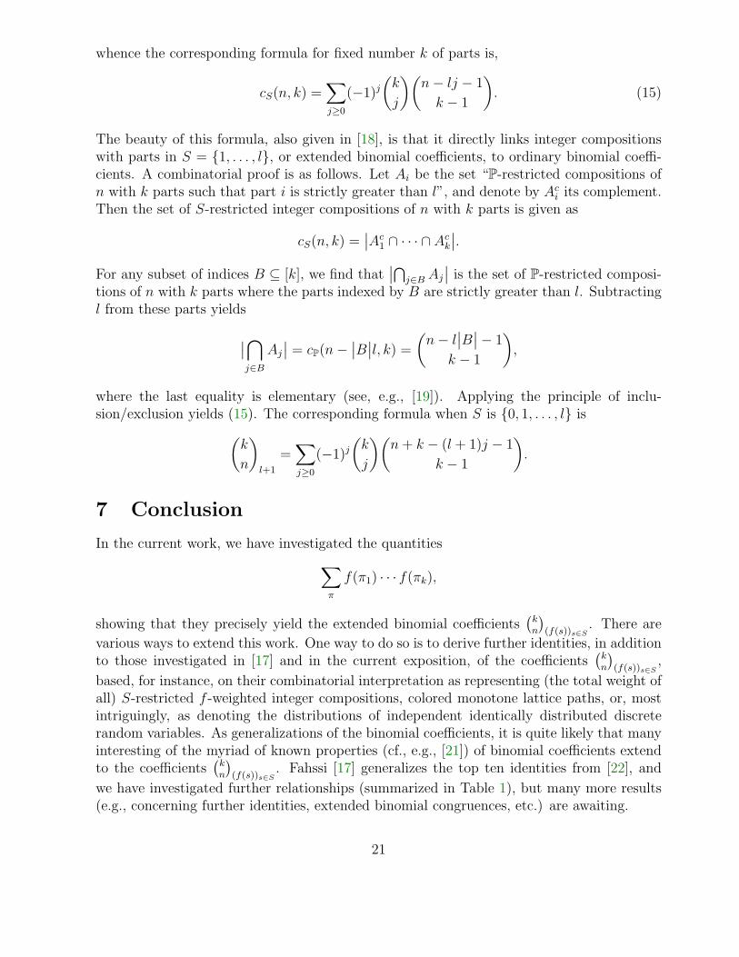
whence the corresponding formula for fixed number k of parts is,
cS(n, k) =∑
j≥0
(−1)j(
k
j
)(
n− lj − 1
k − 1
)
. (15)
The beauty of this formula, also given in [18], is that it directly links integer compositionswith parts in S = {1, . . . , l}, or extended binomial coefficients, to ordinary binomial coeffi-cients. A combinatorial proof is as follows. Let Ai be the set “P-restricted compositions ofn with k parts such that part i is strictly greater than l”, and denote by Ac
i its complement.Then the set of S-restricted integer compositions of n with k parts is given as
cS(n, k) =∣
∣Ac1 ∩ · · · ∩ Ac
k
∣
∣.
For any subset of indices B ⊆ [k], we find that∣
∣
⋂
j∈B Aj
∣
∣ is the set of P-restricted composi-tions of n with k parts where the parts indexed by B are strictly greater than l. Subtractingl from these parts yields
∣
∣
⋂
j∈BAj
∣
∣ = cP(n−∣
∣B∣
∣l, k) =
(
n− l∣
∣B∣
∣− 1
k − 1
)
,
where the last equality is elementary (see, e.g., [19]). Applying the principle of inclu-sion/exclusion yields (15). The corresponding formula when S is {0, 1, . . . , l} is
(
k
n
)
l+1
=∑
j≥0
(−1)j(
k
j
)(
n+ k − (l + 1)j − 1
k − 1
)
.
7 Conclusion
In the current work, we have investigated the quantities
∑
π
f(π1) · · · f(πk),
showing that they precisely yield the extended binomial coefficients(
kn
)
(f(s))s∈S. There are
various ways to extend this work. One way to do so is to derive further identities, in additionto those investigated in [17] and in the current exposition, of the coefficients
(
kn
)
(f(s))s∈S,
based, for instance, on their combinatorial interpretation as representing (the total weight ofall) S-restricted f -weighted integer compositions, colored monotone lattice paths, or, mostintriguingly, as denoting the distributions of independent identically distributed discreterandom variables. As generalizations of the binomial coefficients, it is quite likely that manyinteresting of the myriad of known properties (cf., e.g., [21]) of binomial coefficients extendto the coefficients
(
kn
)
(f(s))s∈S. Fahssi [17] generalizes the top ten identities from [22], and
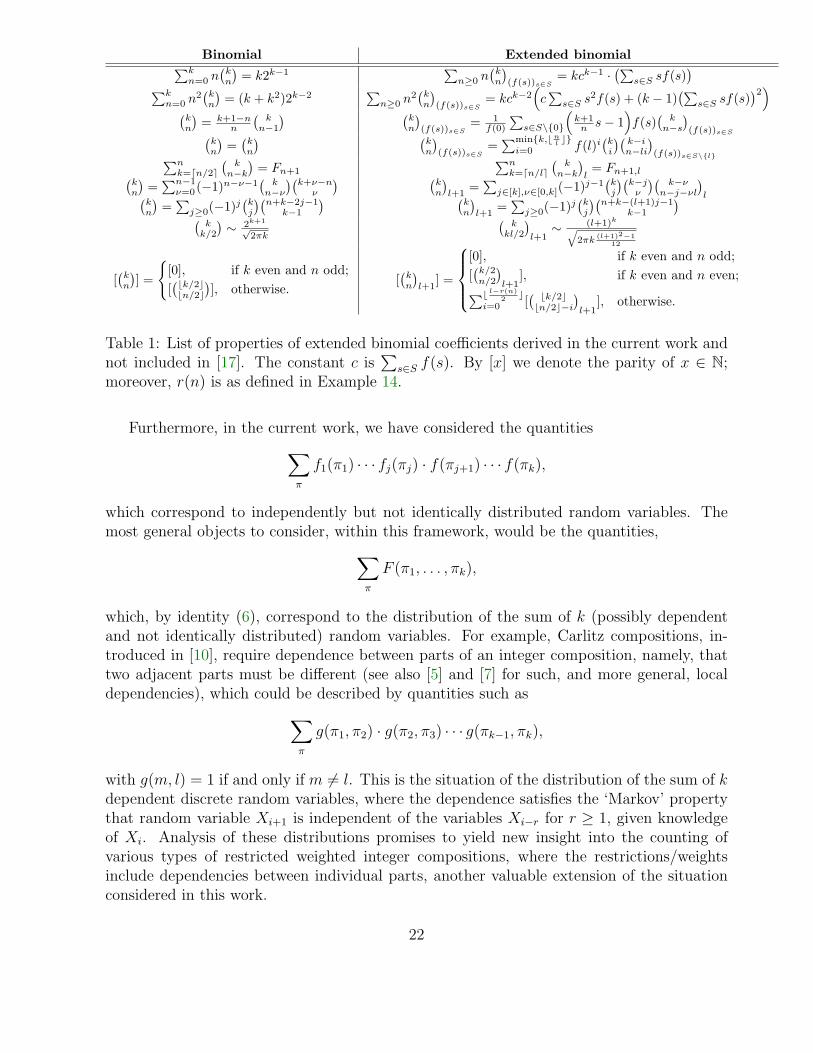
we have investigated further relationships (summarized in Table 1), but many more results(e.g., concerning further identities, extended binomial congruences, etc.) are awaiting.
21
Binomial Extended binomial∑k
n=0 n(
kn
)
= k2k−1∑
n≥0 n(
kn
)
(f(s))s∈S
= kck−1 ·(∑
s∈S sf(s))
∑kn=0 n
2(
kn
)
= (k + k2)2k−2∑
n≥0 n2(
kn
)
(f(s))s∈S
= kck−2(
c∑
s∈S s2f(s) + (k − 1)(∑
s∈S sf(s))2)
(
kn
)
= k+1−nn
(
kn−1
) (
kn
)
(f(s))s∈S
= 1f(0)
∑
s∈S\{0}
(
k+1n s− 1
)
f(s)(
kn−s
)
(f(s))s∈S(
kn
)
=(
kn
) (
kn
)
(f(s))s∈S
=∑min{k,⌊n
l⌋}
i=0 f(l)i(
ki
)(
k−in−li
)
(f(s))s∈S\{l}∑n
k=⌈n/2⌉(
kn−k
)
= Fn+1
∑nk=⌈n/l⌉
(
kn−k
)
l= Fn+1,l
(
kn
)
=∑n−1
ν=0(−1)n−ν−1(
kn−ν
)(
k+ν−nν
) (
kn
)
l+1=
∑
j∈[k],ν∈[0,k](−1)j−1(
kj
)(
k−jν
)(
k−νn−j−νl
)
l(
kn
)
=∑
j≥0(−1)j(
kj
)(
n+k−2j−1k−1
) (
kn
)
l+1=
∑
j≥0(−1)j(
kj
)(
n+k−(l+1)j−1k−1
)
(
kk/2
)
∼ 2k+1√2πk
(
kkl/2
)
l+1∼ (l+1)k
√
2πk(l+1)2−1
12
[(
kn
)
] =
{
[0], if k even and n odd;
[(⌊k/2⌋⌊n/2⌋
)
], otherwise.[(
kn
)
l+1] =
[0], if k even and n odd;
[(
k/2n/2
)
l+1], if k even and n even;
∑⌊ l−r(n)2 ⌋
i=0 [( ⌊k/2⌋⌊n/2⌋−i
)
l+1], otherwise.
Table 1: List of properties of extended binomial coefficients derived in the current work andnot included in [17]. The constant c is
∑
s∈S f(s). By [x] we denote the parity of x ∈ N;moreover, r(n) is as defined in Example 14.
Furthermore, in the current work, we have considered the quantities
∑
π
f1(π1) · · · fj(πj) · f(πj+1) · · · f(πk),
which correspond to independently but not identically distributed random variables. Themost general objects to consider, within this framework, would be the quantities,
∑
π
F (π1, . . . , πk),
which, by identity (6), correspond to the distribution of the sum of k (possibly dependentand not identically distributed) random variables. For example, Carlitz compositions, in-troduced in [10], require dependence between parts of an integer composition, namely, thattwo adjacent parts must be different (see also [5] and [7] for such, and more general, localdependencies), which could be described by quantities such as
∑
π
g(π1, π2) · g(π2, π3) · · · g(πk−1, πk),
with g(m, l) = 1 if and only if m 6= l. This is the situation of the distribution of the sum of kdependent discrete random variables, where the dependence satisfies the ‘Markov’ propertythat random variable Xi+1 is independent of the variables Xi−r for r ≥ 1, given knowledgeof Xi. Analysis of these distributions promises to yield new insight into the counting ofvarious types of restricted weighted integer compositions, where the restrictions/weightsinclude dependencies between individual parts, another valuable extension of the situationconsidered in this work.
22
8 Acknowledgements
The author would like to thank the anonymous referee for many helpful comments.
References
[1] A. K. Agarwal, n-color compositions, Indian J. Pure Appl. Math. 31 (2000), 1421–1427.
[2] G. E. Andrews, Euler’s ‘exemplum memorabile inductionis fallacis’ and q-trinomial co-efficients, J. Amer. Math. Soc. 3 (1990), 653-669.
[3] K. Balasubramanian, R. Viperos, and N. Balakrishnan, Some discrete distributions re-lated to extended Pascal triangles, Fibonacci Quart. 33 (1995), 415–425.
[4] C. Banderier and P. Hitczenko, Enumeration and asymptotics of restricted compositionshaving the same number of parts, Discrete Appl. Math. 160 (2012), 2542–2554.
[5] E. A. Bender and E. R. Canfield, Locally restricted compositions I. Restrictedadjacent differences, Electron. J. Combin. 12 (2005), Paper R57. Available athttp://www.combinatorics.org/Volume_12/Abstracts/v12i1r57.html.
[6] E. A. Bender and E. R. Canfield, Locally restricted compositions II. General restric-tions and infinite matrices, Electron. J. Combin. 16 (2009), Paper R108. Available athttp://www.combinatorics.org/Volume_16/Abstracts/v16i1r108.html.
[7] E. A. Bender and E. R. Canfield, Locally restricted compositions III. Adjacent-part periodic inequalities. Electron. J. Combin., 17 (2010), Paper R145. Available athttp://www.combinatorics.org/Volume_17/Abstracts/v17i1r145.html.
[8] E. A. Bender, E. R. Canfield, and Z. Gao, Locally restricted compositions IV. Nearlyfree large parts and gap-freeness. Electron. J. Combin., 19 (2012), Paper P14. Availableat http://www.combinatorics.org/Volume_19/Abstracts/v19i4p14.html.
[9] C. C. S. Caiado and P. N. Rathie, Polynomial coefficients and distribution of the sumof discrete uniform variables, in A. M. Mathai, M. A. Pathan, K. K. Jose, and J. Jacob,eds., Eighth Annual Conference of the Society of Special Functions and their Applications,Pala, India, Society for Special Functions and their Applications, 2007.
[10] L. Carlitz, Restricted compositions, Fibonacci Quart. 14 (1976), 254–264.
[11] P. Chinn and S. Heubach, (1, k)-compositions, Congr. Numer. 164 (2003), 183–194.
[12] P. Chinn and S. Heubach, Compositions of n with no occurrence of k, in Proceedings ofthe Thirty-Fourth Southeastern International Conference on Combinatorics, Graph Theoryand Computing, vol. 164, 2003, pp. 33–51.
[13] L. Comtet, Advanced Combinatorics, D. Reidel Publishing Company, 1974.
[14] A. De Moivre, The Doctrine of Chances: or, A Method of Calculating the Probabilitiesof Events in Play, 3rd ed., Millar, 1756, reprint, Chelsea, 1967.
[15] N. De Pril, Recursions for convolutions of arithmetic distributions, Astin Bull. 15
(1985), 135–139.
[16] S. Eger, Asymptotic normality of integer compositions inside a rectangle, preprint,http://arxiv.org/abs/1203.0690.
[17] N.-E. Fahssi, The polynomial triangles revisited, preprint,http://arxiv.org/abs/1202.0228.
[18] D. C. Fielder and C. O. Alford, Pascal’s triangle: top gun or just one of the gang?,in G. E. Bergum, A. N. Philippou, and A. F. Horadam, eds., Applications of FibonacciNumbers, Kluwer, 1991, pp. 77–90.
[19] P. Flajolet and R. Sedgewick, Analytic Combinatorics, Cambridge University Press,2009.
[21] H. W. Gould, Combinatorial Identities: A Standardized Set of Tables Listing 500 Bino-mial Coefficient Summations, West Virginia University Press, 1972.
[22] R. L. Graham, D. E. Knuth, and O. Patashnik, Concrete Mathematics, Addison-Wesley,1994.
[23] Y.-H. Guo, Some n-color compositions, J. Integer Seq. 15 (2012).
[24] S. Heubach and T. Mansour, Compositions of n with parts in a set, Congr. Numer. 164(2004), 127–143.
[25] G. Jaklic, V. Vitrih, and E. Zagar, Closed form formula for the number of restrictedcompositions, Bull. Aust. Math. Soc. 81 (2010), 289–297.
[26] D. E. Knuth, The Art of Computer Programming, Vol 2, Seminumerical Algorithms,Addison-Wesley, 1969.
[27] M. E. Malandro, Asymptotics for restricted integer compositions, preprint,http://arxiv.org/pdf/1108.0337v1.
[28] G. Narang and A. K. Agarwal, n-color self-inverse compositions, Proc. Indian Acad.Sci. Math. Sci. 116 (2006), 257–266.
[29] G. Narang and A. K. Agarwal, Lattice paths and n-colour compositions, Discrete Math.308 (2008), 1732–1740.
[30] H. H. Panjer, The aggregate claims distribution and stop-loss reinsurance, Transactionsof the Society of Actuaries 32 (1980), 537–538.
[31] H. H. Panjer, Recursive evaluation of a family of compound distributions, Astin Bull.12 (1981), 22–26.
[32] B. E. Sagan, Compositions inside a rectangle and unimodality, J. Algebraic Combin. 29(2009), 405–411.
[33] E. Schmutz and C. Shapcott, Part-products of S-restricted inte-ger compositions, Appl. Anal. Discrete Math., to appear. Available athttp://pefmath.etf.rs/accepted/rad1442.pdf.
[34] C. Shapcott, C-color compositions and palindromes, Fibonacci Quart. 50 (2012), 297–303.
[35] C. Shapcott, Part-products of 1-free integer compositions, Electron. J. Combin. 18
(2011), #P235.
[36] N. J. A. Sloane, ed., The On-Line Encyclopedia of Integer Sequences, http://oeis.org.
[37] D. P. Walsh, Equating Poisson and normal probability functions to derive Stirling’sformula, Amer. Statist. 49 (1995), 270–271.
Received April 16 2012; revised versions received April 23 2012; September 7 2012; October13 2012; January 3 2013. Published in Journal of Integer Sequences, January 4 2013.