Results Processing in MATLAB for Photonics...

0

Results Processing in MATLABfor Photonics Applications

I.V. Guryev, I.A. Sukhoivanov, N.S. Gurieva, J.A. Andrade Lucioand O. Ibarra-Manzano

University of Guanajuato, Campus Irapuato-Salamanca, Division of EngineeringMexico

1. Introduction

The chapter is intended to provide the reader with powerful and flexible tools based onMATLAB and its open-source analogs for the processing and analyzing the results obtainedby means of highly specialized software.Particularly, in the chapter we give a brief overview of free and open-source as well asshareware software for computation of the photonic crystals characteristics. We concentrateattention mostly to their advantages and drawbacks and give short description of the datafiles they give results in.The next parts of the chapter are dedicated to processing of the results obtained within thespecific software.Firstly, we consider the most basic case of plane results represented by a functionaldependences. In this part, we are talking about the plane data interpolation, approximationand representation.Data interpolation may be used as a tool intended to avoid high resolution computation (whenscanning, say, through the wavelength or frequency) and, therefore, to reduce computationtime which may achieve weeks in the modern numerical problems.Data approximation allows highly efficient data analysis by means of finding the parametersof the target function. For this reason, the numerically obtained data is approximated (withinthe certain accuracy) by the analytical functions including variable coefficients which areusually posses physical meaning. As a result of the approximation, the unknown coefficientsare found.Correct and obvious data representation is very important when writing the scientific paper.Therefore, in the end of current part we give an idea of figure formatting.The next part of the chapter shows reader how to process and represent three-dimensionaland multi-dimensional data. Basically, the operations described for plane data is extrapolatedto multidimensional data arrays.In many cases, the results of the complex numerical research is represented in the form ofmultiple files with similar format. In the next part of the chapter we show how to useMATLAB for merging the data into a single multidimensional array and for representing itin convenient form.

6

www.intechopen.com

2 MATLAB/Book4

The last part of the chapter is dedicated to the animations creation out of multiple instantdata shots. Such form of the data representation is useful when representing time-dependentresults as well as multidimensional data arrays.During all the chapter, we provide reader with working MATLAB codes as well as figuresillustrating the programs results. We believe this information together with learning ofMATLAB fundamentals MATLAB manual (2011) will help young scientists, master and PhDstudents especially in the area of opto-electronics and photonics to analyze and represent theircomputation results in the most effective way.

2. Brief review of the Photonic crystals modeling software

Photonic crystals are optical media possessing the periodic modulation of the refractive index.Due to this, the light behavior inside such structures is similar to the one of the electrons inthe atomic structures (this gives them the name “Photonic crystals”). Main property the PhCspossesses is the photonic band gap (PBG) which is an optical analog of the electronic bandgap in semiconductor materials.Depending on the geometrical peculiarities, the PhCs are subdivided to several categories.Particularly, there are wide classes of 1D, 2D and 3D PhCs classified by number of dimensionswhere the variations of the refractive index appear. These classes, in turn, are dividedaccording to the lattice type, existence or absence of the PBG, etc.The physical principles of the PhCs are well-known and are considered in numerous articlesand books Joannopoulos et al. (1995), Lourtioz et al. (2005), Sakoda (2001). There existnumerous methods for modeling the PhC characteristics, which are well described Sakoda(2001), Taflove & Hagness (2005) and are implemented in a numerous software products. Thischapter is considered by us as a natural addition to the book Sukhoivanov & Guryev (2009)which describes computation methods of the PhCs characteristics. It is intended to extendand improve the efficiency of the results representation.Particularly, this section is dedicated to brief introduction into freeware and sharewaresoftware for PhC and PhC-based devices basic modeling.Since the PhC-based devices are investigated intensively today, the crucial moment is the rightchoice of the computational methods which are implemented in a number of software.Particularly, the development of the PhC devices require detailed analysis of the PhCeigenstates (or resonant frequencies) as a dependence of the direction of the light propagation.This kind of tasks may be done by means of different methods like analytical one (however, for1D PhC only), finite differences time domain (FDTD) method, finite elements method (FEM),plane wave expansion method (PWE). Each method has its advantages and drawbacks, theyall require different computation time and accuracy and are implemented in a different kindsof software.The other important problem for PhC investigation is the computation of the field distributioninside the defined structure. Again, in the simplest cases (particularly, in case of 1D PhC withpassive optical materials) the field distribution can be found analytically. However, in themost cases the numerical methods are required such as FDTD, FEM, PWE, etc.Most of the software (especially, free ones) are intended to implement all the aspects of asingle methods. However, professional shareware soft implements several different methodsallowing the user to investigate the device from different points of view.

120 MATLAB for Engineers – Applications in Control, Electrical Engineering, IT and Robotics

www.intechopen.com

Results Processing in MATLAB

for Photonics Applications 3

2.1 Free and open-source software

Within all the variety of the scientific software available, the developers are allowed to choosebetween low price and friendly interface. The friendly interface provides the user with a lotof default settings and saves a lot of time which may be spent to the research problems. Onthe other hand, being more complicated for user, free software requires deep knowledge ofphysical and mathematical aspects of the investigated area (which is considered by authorsas an advantage of free software). Particularly, the scientist intended to investigate the opticalproperties of the periodic structures has to be well-educated in the fields of solid-state physics,electromagnetism, numerical methods, etc. Having these knowledge, the user may define theproblem more precisely and carry out the research at higher level with deeper understandingof the matter of the problem.Therefore, this part of our review is dedicated to the software which is available online andmay be easily tested and learned by reader.

2.1.1 MPB

The MIT Photonic Bands (MPB) MPB (2011) software is one of the most powerful toolsavailable freeware which is intended to compute the eigenstates of the photonic crystal ofdifferent configurations by means of PWE method. It is written by developers of the PhCtheory whose investment into the physics of PhC devices was critical. Therefore, the MPBsolves the problems in a most suitable way for the scientists.However, since MBP runs script files with detailed description of the structure andcomputation conditions, using of the MBP requires from user high skills, particularly,in solid-state physics and turns computation of even the simplest case into a seriousprogramming task. Several examples provided with the installation help to understand theprinciples of the structure setup and they may be used as a default structures which is easy tomodify and use for other structures.The program outputs results into console which allows to read them but not analyze.Therefore, file output should be used. Particularly, the field distribution is being outputinto HDF5 format which is supported by visualization tools like h5utils. However, even forsimple analysis, approximation and decoration the user has to use additional software suchas MATLAB.

2.1.2 MEEP

Meep (or MEEP) MEEP (2011) is a free finite-difference time-domain (FDTD) simulationsoftware package developed at MIT to model electromagnetic systems.It can be used to successfully compute electromagnetic field distribution inside thePhC-devices made either of linear or nonlinear materials (possessing Kerr of Pockelsnonlinearities).

2.2 Shareware software

In contrast to free software, the shareware ones have, in most cases, highly advanced userinterface which helps novice to study the new soft and, on the other hand, saves professionals’time keeping them from the necessity of learning side skills such as programming.As for the PhC modeling, the most advanced computation tools available on the markets areRSoft (namely, BandSolve and FullWave) and Comsol Multiphysics (namely, RF module).

121Results Processing in MATLAB for Photonics Applications

www.intechopen.com

4 MATLAB/Book4

2.2.1 RSoft

RSoft RSoft (2011) being developed by the RSoft-group for many years and it have come along way since its earlier versions to its modern view.Though its interface has been changed from version to version, it uses the same methods forcomputation of the PhC characteristics. Namely, BanSolve module allows one to compute theband structures of the PhC as well as its modes’ field distribution by means of PWE methodwhile FullWave implements FDTD method applying it to the field distribution computationinside the arbitrary structures and, in special case, the band structure.The RSoft interface provides user with many useful models generated with defaultparameters. Moreover, wise linking to the variables allows flexible modifications of thedefault structures. This allows you to create the simple structure in a several mouse clicks andmore advanced structures in several minutes. Among the drawbacks of the interface it shouldbe mentioned too simple 3D structure definition which does not allow visual representationof the structure. To do this, additional software such as MayaVi should be used.Except the possibility of modifying the structure with variables, RSoft’s dialog boxes providedozens of visual controls allowing definition of an arbitrary structure, computation conditionsand the output information.It should also be mentioned the graphic output of the RSoft. Although it allows analyze thecomputation results, their quality is unsatisfactory and one have to use additional software tomake results representation suitable for publications. Moreover, in case of FullWave module,continuous graphic output essentially slows down the computation process.In general, the RSoft is a powerful PhC modeling tool which allows solution of wide rangeof problems. However, results output is performed into the data files only and requiresadditional postprocessing, particularly, with Matlab.

2.2.2 Comsol Multiphysics

The Comsol Multiphysics COMSOL (2011) (previously known as Femlab) allows solvingwide variety of problems defined by the partial differential equations in a number of fieldsof Physics by means of FEM. Particularly, in the area of PhC devices it allows to solve theHelmholtz equation with certain kinds of boundary conditions, thus, giving as a result theelectromagnetic field distribution inside the device.The structure definition as well as setting the properties of the structure, boundary conditionsand node conditions are highly visualized and it makes no difficulties in creating computationmodel.As for results representation, Comsol Multiphysics provides a lot of different visualizationmodes in form of 2D, 3D, contour, etc., thus, making for user unnecessary to deal withvisualization of quite complicated data structures.However, field distribution and basic data analysis is not always enough for serious scientificresearch. In case the PhC device has complex structure and requires detailed analysis of thefield distribution (like confinement factor of the waveguide), the output files data should beinvestigated separately.Therefore, independent on the convenience of the software itself, the problem of the outputdata processing is always arising and the best way to carry this out is by means of MATLAB.


www.intechopen.com



3. Data files formats

As a result of computation of any PhC characteristic such as band structure, field distribution,temporal response, etc., the data is alway represented in some special format which can beread and processed with MATLAB.With simulation software you may obtain several different kinds of data files, namely, theplane data (two-coordinate dependence), 3D data (tree-coordinate dependence), random data(where data points are linked to the mesh nodes), structured data (the data is represented inthe form of known structures), multiple files data (usually, the parametric data where each filecorresponds to the solution with a single value of the parameter).

3.1 Reading plane data

The data represented in a plane form usually represents the tabulated function of one variableand is really the simplest data format. In many cases, the computational programs output thedata in a form of two rows as presented in figure 1

Fig. 1. The example of the plane data file

In the one wants to plot or process this kind of data, then it can be easily read by MATLABscript using a single command:

varName=load(fileName, ’ ASCII’ )

After this, the variable varName contains an array Nx2.However, in some cases, the plane data file has the text header before the data itself (see figure2 which demonstrates the data where the first line is a text header). This causes the problemsince the data cannot be read with load command from the MATLAB. One of the solution is touse the Import Data dialog (Menu File/Import Data. . . ) which performs smart data analysisand separates the numerical data from the text one.On the other hand, it is more suitable to integrate the data import procedure into the scriptin order to avoid manual operations and, to be able to perform multiple import operationswhen processing multiple data files. For this reason, we have to use standard data readingoperations to analyze file. The drawback of this method is necessity to know exactly the filestructure, namely, how many strings takes the text header. Here is the simple example ofopening the file generated by RSoft and having the text header.


www.intechopen.com

6 MATLAB/Book4

Fig. 2. The example of the data file containing text header

%Code for reading the data file containing text header

%opening the filefile=fopen(’scan_gaps_TE.scn’ );

%skipping the file header (this part should be modified according%to the specific file format)fscanf(file,’%s’ ,9);

%Reading the first line of the data.%variable ’read’ contains the data from the read string,%variable ’num’ contains the number of variables actually read.%the length of the array to read to should be selected according%to the dimensions of the data in the file[read, num]=fscanf(file,’%f’ ,[1,8]);

%Resetting the counter to write into the data arraycounter=1;

%main reading cycle. Executes while the data read from the file%contains actual data (num>0)while(num)

%copying the data from temporary variable into the data%variabledata(counter,:)=read;

%increasing the counter valuecounter=counter+1;

%reading the next line from the file[read, num]=fscanf(file,’%f’ ,[1,8]);


www.intechopen.com



end

%closing the data filefclose(file);

This code opens the data file as a regular file and then uses the function scanf() to read thedata of the certain format. Particularly, for the file presented in the figure 2 it first reads 9strings separated by the whitespaces and then reads each line containing 8 numbers into anarray 1x8. Then in the cycle it copies each row into the resulting 2D array.In case of plane data, each column has its meaning and have to be treated by the programaccordingly. For instance, in case of the RSoft file generated by the scanning the full photonicband gaps (PBG) over some parameter, the first row indicates the value of the parameter, thesecond one is for the number of the PBG starting from the one with the lowest frequency, thethird is for the central frequency of the PBG and so on. Detailed information on the specificfiles formats is usually contained in the manual for the specific software.

3.2 Reading 3D data

3D data is represented in the file in form of 2D array. In this case, each dimension of the arraycorresponds to the space dimension and, therefore, each number placed in the position (X,Y)in the file is treated as an altitude of the point with coordinates (X*scale,Y*scale). The value ofthe variable ’scale’ depends on the physical dimensions of the structure.Usually, reading of the 3D data does not differ from reading the plane data. In case of fileswithout headers, the data is read by a simple load() function of the MATLAB. The scale ofthe structure should be known in this case to be able to assign physical coordinates to thepositions in the array.However, in case of the header presence, we have to use the method described in thesubsection 3.1 for plane data. In this case the header may contain useful information suchas linking to the physical dimensions, position of the structure, etc (see figure 3).

Fig. 3. The 3D data file with header


www.intechopen.com

8 MATLAB/Book4

In this case, instead of just skipping the header block, we can extract useful information fromit. The following code demonstrates how to read and analyze the header info when drawingthe field distribution computed by RSoft:

%Opening the data filefff=fopen(’field.fld’ );

%Skipping two lines containing picture formatting info%(namely, two strings separated by the <CR>)fscanf(fff,’%s’ ,2);

%Reading contents of the numerical part of the header into%variable ’field_info’field_info=fscanf(fff,’%i %f %f %f OUTPUT_REAL_3D\n %i %f %f \n’ ,7);

%using the variable ’field_info’ to read properly formatted%data on the field distributionfield=fscanf(fff, ’%f’ , [field_info(5), field_info(1)]);

Here, after opening the file, we are skipping two strings which mean nothing for us. Thenwe read all the numerical values into the array and can use this variable to determine thedimension of the array, the physical size of the computation region, etc.

3.3 Reading the random data

Using the header to define the parameters of the figure is not always enough. Particularly, itworks for the uniformly distributed data points such as in FDTD method. However, if you useFEM, for example, Comsol Multiphysics, you will deal with non-uniform triangular mesh. Inthis case, the data is organized into structured. Each unit contains X and Y coordinate (in caseof 2D model) or X, Y and Z coordinate (in case of 3D physical model) and the value of the fieldintensity corresponding to this point (see figure 4).

Fig. 4. The file containing random data linked to the specific points of the mesh

Reading of the date in this case is performed just as in case of the plane data, however, onehave to fill two or three coordinate arrays X, Y and possibly Z, and the array of correspondingvalues of the field intensity.It is also possible to convert this data into a regular mesh data which will be described infollowing section.

3.4 Reading structured data

In case of MPB and MEEP software, the field distribution is being output in so-called HDF5format which is supported by many visualization tools as well as programming languages.


www.intechopen.com



Particularly, in MATLAB there is a set of functions providing correct work with the HDF5. TheMATLAB command HDF5Read(...) reads the contents of the file into the structure from whereit can be easily extracted by standard structure addressing command (in case of MATLAB it isthe dot operator). Here is simple MATLAB program which reads results computed by MEEPfrom HDF5 file and analyzes parameters of the results.

%Program allows reading from the the .h5 file containing the results of the%field distribution computed with MEEP

clear all

%The function hdf5info allows obtatining the information from the .h5 file%required to read the actual datahinfo=hdf5info(’/home/igor/temp/wg_bend ez.h5’ );

%Then we are reading the information using the query string from the hinfo%structureres=hdf5read(hinfo.GroupHierarchy.Datasets(1));

%In this particular case, the computation results contain several frames%with field distribution at different moments of time. The cycle reads them%from the data structure and then draws.for i=1:(size(res))(1)

%Copying the frame into a separate 2D arraydrawres(:,:)=res(i,:,:);

%Drawing the frameimage(drawres∗1000);colormap(’gray’ );

%Drawing immediatelydrawnow;

end

However, as it have been described in the previous section, the data in the files may berepresented in the forms of an arbitrary structures which requires a lot of work to dig in andto write corresponding unique decoders.

3.5 Reading multiple files data

In many cases, when you perform the parametric computations, the results have form ofmultiple files. Each file corresponds to a single value of the parameter and may have oneof the formats described earlier.The main problem in this case is to gather the data from all the files into a single data structure.This problem will be discussed in the following section. Here we will focus on how to openmultiple files. The following piece of code shows how to open the files which have similarnames with a counter attached to them:


www.intechopen.com

10 MATLAB/Book4

%Scanning over all the numbers of the filesfor num=0:90

name=strcat(path,’metadata’ ,num2str(num,’%02i’ ),’.dat’ )

clear temporal_response;temporal_response=load(name, ’ ASCII’ );

%Here performing all the operations we need... ...

end

We presume to have file names in the following form: “metadata00.dat”, “metadata01.dat”,“metadata02.dat”,. . . ,“metadata90.dat”. In this code, the outer loop scans over all thenumbers from 0 to 90. The function strcat() allows concatenating several strings into oneand generate the name. Using the function num2str() we convert the numerical type into astring.The problem, may appear with the filenames since for the numbers lower than 10 we havezero-filler in the name. We can fix the problem in two different ways. The first one is justto compare the variable ’num’ with 10 and if it’s lower than 10, just to add ’0’ to the stringmanually. However, this is a solution only in particular cases. Suppose, you have numbersfrom 0 to 100000. In this case, you will have to make 5 different comparisons each for one digit(num < 10, num < 100, num < 1000, num < 10000, num < 100000). This is already a sort ofannoying and far from elegance.The second possible solution is to use formatted conversion of the number. In this case wejust have to use format string “%02i” to fill the spaces before the number with zeros. Herethe symbol of “%” tells MATLAB about the beginning of the format string, following “0”makes MATLAB to fill the spaces with zeros, “2” tells exactly how many digits it is supposeto be in the number and “i” indicates integer data type. Detailed information about the stringformatting can be found in the MATLAB documentation in the section of the function fprintf().

4. Processing plane data

The plane numerical data is represented by two arrays, one of which contains values alongone coordinate axis while another one corresponds to another axis. This simplest form of thedata representation is actually the most clear and understandable when you want to presentyour results.However, in some cases direct plotting of the data is not really representable. Particularly,when you make an expensive experimental research like temporal response measurement ofthe nonlinear PhC using ultra-short pulses, or when you perform the computation which is sotime- and resource-consuming that you are unable to obtain sufficient number of data pointslike, for instance, computation of the photonic band gap maps. In these cases, before to createthe data output, you have to convert it, improve it or make some other handling. This sectionis dedicated to the manipulations on the data which allow to improve its representation.


www.intechopen.com



4.1 Data interpolation

The interpolation is the most useful operation on the data obtained during the experimentalresearch on numerical computation. In the mathematical subfield of numerical analysis,interpolation is a method of constructing new data points within the range of a discreteset of known data points. There are a lot of different ways to interpolate the data likelinear interpolation, polynomial interpolation, spline interpolation, etc. We will not considermathematical side of the interpolation process concentrating on the implementation of thisoperation in MATLAB.For the interpolation of the plane data, MATLAB uses the function interp1(). As an inputarguments, the function has initial X and Y values of the data as well as new values of X atwhich you want to obtain the new values. It is also possible to select the interpolation method.As an output, this function returns the new values of Y found by interpolation process.Here is the simple example of the data interpolation. In this example, we have the dependenceof the photonic band gap width of the 1D PhC on the layer width. The data points arecalculated for the limited number of values of the witdh. However, due to interpolation,we have smooth curve which looks much nicer.

%The program demonstrates different interpolation techniques%performed by MATLAB. The interpolation is applied%to the dependence of the photonic band gap width of 1D PhC on the%layers witdh

%Loading the information on the PBG width from the filedata=load(’pbg_width.dat’ ,’ ASCII’ );

%Getting the values of X from the data arrayx=data(:,1)’;

%Getting the values of Y for the second band (third column)%in the datafiley=data(:,5)’;

%Creating the mesh 10 times more dense which is required%for interpolationx1=interp1(1:length(x),x,1:0.1:length(x));

%Creating new figurefigure;%Drawing at the same figurehold on;%Using the function interp1, interpolating the data with nearest valuesy1=interp1(x,y,x1,’nearest’ );%Plotting the initial data with blue round markersplot(x,y, ’bo’ , ’LineWidth’ ,2);%Plotting the interpolated data with grin solid lineplot(x1,y1, ’g’ , ’LineWidth’ ,2);

%Doing the same with linear interpolation


www.intechopen.com

12 MATLAB/Book4

figure;hold ony1=interp1(x,y,x1,’linear’ );plot(x,y, ’bo’ , ’LineWidth’ ,2);plot(x1,y1, ’g’ , ’LineWidth’ ,2);

%Doing the same with spline interpolationfigure;hold on;y1=interp1(x,y,x1,’spline’ );plot(x,y, ’bo’ , ’LineWidth’ ,2);plot(x1,y1, ’g’ , ’LineWidth’ ,2);

%Doing the same with cubic interpolationfigure;hold on;y1=interp1(x,y,x1,’cubic’ );plot(x,y, ’bo’ , ’LineWidth’ ,2);plot(x1,y1, ’g’ , ’LineWidth’ ,2);

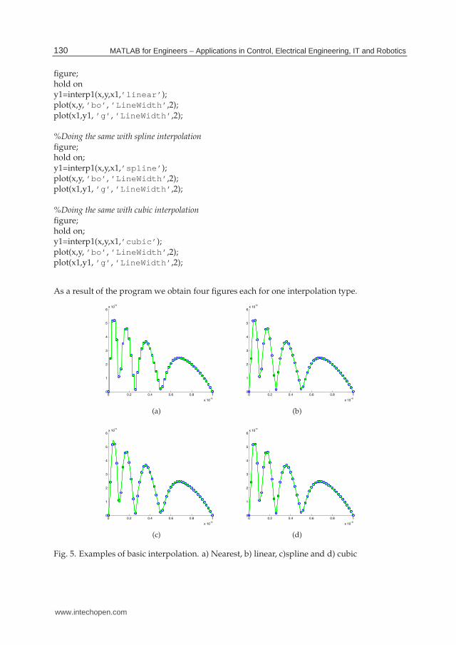
As a result of the program we obtain four figures each for one interpolation type.

0 0.2 0.4 0.6 0.8 1

x 10−6

0

1

2

3

4

5

6x 10

14

(a)

0 0.2 0.4 0.6 0.8 1

x 10−6

0

1

2

3

4

5

6x 10

14

(b)

0 0.2 0.4 0.6 0.8 1

x 10−6

0

1

2

3

4

5

6x 10

14

(c)

0 0.2 0.4 0.6 0.8 1

x 10−6

0

1

2

3

4

5

6x 10

14

(d)

Fig. 5. Examples of basic interpolation. a) Nearest, b) linear, c)spline and d) cubic


www.intechopen.com



In the program, the interpolation is performed in four different ways provided by MATLAB(actually, there are also “pchip” and “v5cubic” types. However, pchip is similar to cubic andv5cubic is just an old version of cubic). From the results, it is seen that for the selected curvethe best interpolation technique is a spline interpolation.

4.2 Data approximation

Data approximation is an operation which allows to describe (approximate) the tabulated databy an analytical function.The approximation is always used when the general view of the analytical dependencecan be predicted, however, the coefficients still remain unknown. This is usually happensin the experimental researches when it is necessary to determine the parameters of theanalytical dependence. Particularly, when the experiment is intent to determine the effectiverefractive index of the PhC by measuring the radiation deviation at different wavelength.After the experiment, the data is approximated by parametric analytical function where theparameter is the effective refractive index. The best approximation result gives the value ofthe mentioned parameter.In MATLAB there is a separate toolbox providing the approximation of the tabulated data,namely, the Curve Fitting Toolbox. And again, using of the toolbox is possible in a singlecase only. However, using the toolbox requires definite time and when you need to performmultiple operations, this turns into a mess.In this section we describe how to approximate the data in MATLAB without using thetoolbox. The following program generates randomly five points and then approximates themwith polynomial function of the fourth order.

%This function approximates five random points with 4 th order%polynomial function. Since 4 th order polynom allows exact approximation,%the error should be absent.

function approximation_plane%Creating five X valuesx=1:5;

%Randomly generating 5 Y valuesy=rand(1,5)∗10;

%Creating the initial values for approximation processstart=[1 1 1 1 1];

%Starting five minimization interationsfor i=1:5

%Using the function fminsearch() to optimize the ’coefs’ a the selected%points (X, Y)estimated_coefs = (fminsearch(@(coefs)fitfun(coefs,x,y),start));

%changing the starting values to the optimized ones and then starting%overstart=estimated_coefs;


www.intechopen.com

14 MATLAB/Book4

end

%Building the smooth analytical function with coefficients obtained during%optimization processx1=0:0.1:6;y1=analyt_fn(estimated_coefs,x1);

%Creating the figurefigure;hold on;%Plotting the initial pointsplot(x,y,’bo’ ,’LineWidth’ ,2);%and the smooth analytical functionplot(x1,y1,’g’ ,’LineWidth’ ,2);

%In the title writing the final polynomtitle(strcat(’y=’ ,num2str(estimated_coefs(1)),’ \cdotxˆ4+(’ ,...

num2str(estimated_coefs(2)),’) \cdotxˆ3+(’ ,...num2str(estimated_coefs(3)),’) \cdotxˆ2+(’ ,...num2str(estimated_coefs(4)),’) \cdotx+(’ ,...num2str(estimated_coefs(1)),’)’ ),’FontSize’ ,16);

%Function for optimizationfunction err=fitfun(coefs,x,y)

%The function returns the difference between the analytical function%with coefficients ’coefs’ at points X and the actual values of Yerr=norm(analyt_fn(coefs,x) y);

end

%Analytical parametric function to be optimizedfunction analyt_fn=analyt_fn(coefs,x)

analyt_fn=coefs(1)∗x.ˆ4+coefs(2)∗x.ˆ3+coefs(3)∗x.ˆ2+coefs(4)∗x+coefs(5);end

end

The result of the function work is presented in figure 6. It can bee seen that approximation isquite accurate.For the optimization procedure, MATLAB uses simplex search method which is implementedin the form of function fminsearch(). As an input parameters it has a pointer to a function tobe minimized and the initial values of the parameter. In our case, the function to minimizereturns the difference between actual points and the analytical function which, in turn, isdefined in the function analyt_fn().It should be paid attention to the fact that in current example the polynomial function of thefourth power approximates five data points. In this case, there is only one strict solution.However, in most cases, the approximation is made with certain accuracy which should beproperly estimated. The best way to estimate the accuracy is to measure minimum, maximumand avarage deviation.


www.intechopen.com



0 1 2 3 4 5 6−10

0

10

20

30

40

50

60

70

80

y=1.3917⋅x4+(−17.599)⋅x

3+(76.4662)⋅x

2+(−130.3002)⋅x+(1.3917

Fig. 6. Result of approximation of the data by the polynomial function

As an example, we give the code which approximates the dependence of central frequencyof the photonic band gap of 1D PhC on the layer width, with hyperbolic function andestimates the approximation error. The data is obtained by means of plane wave expansionmethod Sukhoivanov & Guryev (2009) with low accuracy. With approximation it is possibleto determine the analytic function describing such a dependence.Consider the following code:

%This function approximates the dependence of the central%wavelength of the photonic band gap of 1D PhC on the layer%width with hyperbolic function.%It also performs the error estimation.

function approximation_plane_err_estimation%Loading information about the central frequency of the%bandgap of 1D PhC from the filedata=load(’pbg_center.dat’ ,’ ASCII’ );

%Getting the values of X from the data arrayx=data(:,1)’;

%Getting the values of Y for the second band (third column)%in the datafiley=data(:,3)’;

%Creating the initial values for approximation process%Now there’s only four values since we use 3 rd order polynomstart=[1e14 0];

%Using the function fminsearch() to optimize the ’coefs’ a the selected%points (X, Y)estimated_coefs = (fminsearch(@(coefs)fitfun(coefs,x,y),start));


www.intechopen.com

16 MATLAB/Book4

%Building the smooth analytical function with coefficients obtained during%optimization processx1=interp1(1:length(data(:,1)),data(:,1),1:0.1:length(data(:,1)));y1=analyt_fn(estimated_coefs,x1);

%using the function ’find’ searching for indices of the refined X values%which are equal to the initial ones[row est_ind]=find(meshgrid(x1,x) meshgrid(x,x1)’ == 0);

%Searching for minimum deviation of the analytical function from the initial%data (using est_index to compare corresponding points)minerr=min(abs(y1(est_ind) y));

%In the same manner, searching for maximum deviationmaxerr=max(abs(y1(est_ind) y));

%Calculating avarage erroravgerr=sum(abs(y1(est_ind) y))/length(y)

%Creating the figurefigure;hold on;

%plotting the solutionplot(x,y,’bo’ ,’LineWidth’ ,2);%and the smooth analytical functionplot(x1,y1,’g’ ,’LineWidth’ ,2);

%Writing the error values at the figuretext(min(x1),min(y1)+(max(y1) min(y1))/10,...

strcat(’Minimum error = ’ , num2str(minerr,’%.2e’ )),’FontSize’ , 14);text(min(x1),min(y1)+(max(y1) min(y1))/10∗2,...

strcat(’Maximum error = ’ , num2str(maxerr,’%.2e’ )),’FontSize’ , 14);text(min(x1),min(y1)+(max(y1) min(y1))/10∗3,...

strcat(’Avarage error = ’ , num2str(avgerr,’%.2e’ )),’FontSize’ , 14);

%Creating the title to the figuretitle(strcat(’y=’ ,num2str(estimated_coefs(1),’%.2e’ ),’/(x+’ ,...

num2str(estimated_coefs(2),’%.2e’ ),’)’ ),’FontSize’ ,16);

%Function for optimizationfunction err=fitfun(coefs,x,y)


www.intechopen.com



%The function returns the difference between the analytical function%with coefficients ’coefs’ at points X and the actual values of Yerr=norm(analyt_fn(coefs,x) y);

end

%Analytical parametric function to be optimizedfunction analyt_fn=analyt_fn(coefs,x)

analyt_fn=coefs(1)./(x+coefs(2));end

end

0 0.2 0.4 0.6 0.8 1

x 10−6

0.6

0.8

1

1.2

1.4

1.6

1.8

2x 10

15

Minimum error =6.10e+10

Maximum error =4.70e+13

Avarage error =1.45e+13

y=9.36e+08/(x+4.93e−07)

Fig. 7. Displaying the approximation accuracy information

Now the result is represented in the form shown in the figure 7. We currently used thehyperbolic function which gave good agreement with numerical results. In this case, not allthe points (in general case, neither of them) are fall at the analytical curve. Thus, estimatingthe error, we are able to confirm the validity of the approximation. In case of large error value,the function is unable to approximate the data at any conditions. This may happen when youhave selected wrong kind of approximating function or, in case of too complex function, haveselected wrong values of the initial parameters.

4.3 Data representation

In the scientific publication the data representation plays main role when it comes to correctunderstanding of the computation or experimental results. In two previous subsections wehave described the way for data interpolation and approximation which helps to performthe data analysis as well as smooth the data. However, the data presentation is alsoimportant. Some basic techniques have already been used earlier without explanation such asmanipulation of the figure’s and plot’s parameters. In this subsection we will try to describeand explain the most useful of them.First thing which should be known about MATLAB, it is the object-oriented environment.This means that after creating some object such as plot, text, line, etc., they can be modifiedand their properties can be easily changed.As always, the most simple way to manipulate the objects parameters is to use visualenvironment provided by MATLAB. For this reason, it is enough just to double-click at someobject while editing mode is active (for this, you have to press the mouse pointer icon at the


www.intechopen.com

18 MATLAB/Book4

(a) (b)

Fig. 8. Visual editing of the object’s properties

tool panel). After this, you will see the editing panel which allows editing some parametersof the selected object (see figure 8(a)).Deeper understanding of the parameters of the objects can be achieved when openingadditional parameters panel or properties inspector (see figure 8(b)). Here you can see andedit all the parameters available for the object.However, editing parameters inside your script is the most fast and productive way to changethe figure appearance (imagine that you have to redraw the figure over and over and modifydozens of parameters manually).There are two ways to set up the parameters of the objects. The first one is to set them onthe stage of their creation. And the second one is modify them after the object is created withdefault properties.In the first method, the parameters are transfered as arguments to the function which createsan objects like in following code:

%Approximation process.........


www.intechopen.com



%Plotting the initial dataplot(x,y, ’LineWidth’ , 2, ’LineStyle’ , ’none’ , ’Marker’ , ’o’ , ’Color’ , ’k’ );%Plotting the approximated dataplot(x1,y1,’LineWidth’ ,2, ’LineStyle’ , ’ ’ , ’Color’ , [0 0.3 1]);

%Adding the text markstext(min(x1)+0.1,min(y1)+(max(y1) min(y1))/10,...

strcat(’Minimum error = ’ , num2str(minerr)),’FontSize’ , 14);text(min(x1)+0.1,min(y1)+(max(y1) min(y1))/10∗2,...

strcat(’Maximum error = ’ , num2str(maxerr)),’FontSize’ , 14);text(min(x1)+0.1,min(y1)+(max(y1) min(y1))/10∗3,...

strcat(’Avarage error = ’ , num2str(avgerr)),’FontSize’ , 14);

Here we show more advanced plotting from the approximation example. Pay attentionthat after plotting the data (X-values and Y-values), we place a lot of textual and numericalparameters. Parameters are usually defined by a pair name-value. The value can be a string,a number or an array depending on the parameter’s requirements.Particularly, the first plot function will draw the data with the LineWidth=2 (initially its 0.5),without the lines connecting the data points (LineStyle=none), but with circular markers(Marker=o) drawn with black color (Color=k).The second plot draws the approximated data with LineWidth=2, with dashed line(LineStyle=’–’) and with color defined by three RGB values (each value varies from 0 to 1).The text marks have only the parameters Fontsize=14.As we have mentioned previously, there is another way to change the parameters of the objectsusing the object identifier. Note that each function which creates an objects, also returns anobject identifier which can be stored into a variable and used lately to manipulate the object.Particularly, the properties of the object can be easily changed using the function set() whichhas as a parameters the object identifier and the set of object’s properties. Consider this simpleexample which makes the same as previous one but modifying the properties after the objectis created:

%Approximation process.........

%Plotting the initial datap1=plot(x,y);set(p1, ’LineWidth’ , 2, ’LineStyle’ , ’none’ , ’Marker’ , ’o’ , ’Color’ , ’k’ );

%Plotting the approximated datap2=plot(x1,y1);set(p2,’LineWidth’ ,2, ’LineStyle’ , ’ ’ , ’Color’ , [0 0.3 1]);

%Adding the text markst1=text();set(t1, ’Position’ ,[min(x1)+0.1,min(y1)+(max(y1) min(y1))/10,0],...


www.intechopen.com

20 MATLAB/Book4

’String’ ,strcat(’Minimum error = ’ , num2str(minerr)),...’FontSize’ , 14);

t2=text();set(t2, ’Position’ , [min(x1)+0.1,min(y1)+(max(y1) min(y1))/10∗2,0],...

’String’ ,strcat(’Maximum error = ’ , num2str(maxerr)),...’FontSize’ , 14);

t3=text();set(t3, ’Position’ , [min(x1)+0.1,min(y1)+(max(y1) min(y1))/10∗3,0],...

’String’ ,strcat(’Maximum error = ’ , num2str(avgerr)),...’FontSize’ , 14);

This code does exactly the same as previous one, however with significant difference. Whenthe function creating the object is called, the object identifier is stored into a correspondingvariable. After this, the function set() is called to modify the objects properties. Pay attention,in case of text labels, the object is created with default properties. All the properties includingthe text strings are set later using the identifiers.This code seems to be unnecessarily more awkward then the previous one but actually, ithas one great advantage. After you stored the variable identifier, you are able to manipulatethe object in any way you want. Particularly, you can easily create an animation by varyingthe parameters of the object (such as camera view) in a loop and saving each frame (forinformation about animations see the last section).

5. Simple 3D data processing

Operating with 3D data is more complicated than with plane one. Particularly, the mostsimple data to be work with is data organized into a regular 2D mesh such as results of FDTDcomputation. However, in some cases it is important to perform the data interpolation.

5.1 Data on rectangular mesh

The most frequently, the data organized into a rectangular mesh may be found in the fielddistribution output of the software implementing the FDTD method. However, each of theprograms creates its own data format and, therefore, should be treated individually. Here asan example, we will give the programs reading the data from RSoft and MEEP.

5.1.1 Processing the data from RSoft

When the RSoft outputs the field distribution, it usually created two different files. The firstone contains the field distribution and the second one contains the information about thestructure boundaries. Therefore, it is necessary to read both files for correct representation thecomputed data.Consider the following code for reading the RSoft field output:

%The program draws the field distribution computed by RSoft%Over the field distribution it draws the structure which is%read from the file generated by RSoft

clear all


www.intechopen.com



%The variable ’name’ contains filename without the extensionname=’field_high_state’

%Opening the file containing the field infofff=fopen(strcat(name,’.fld’ ));

%Skipping the inforation about the plotting%which is unuseful for usfscanf(fff,’%s’ ,2);

%Into the variable ’field_info’ reading useful informationfield_info=fscanf(fff,’%i %f %f %f OUTPUT_REAL_3D\n %i %f %f \n’ ,7);

%Reading the data points into 2D array. The dimensions of the%array are taken from the variable ’field_info’field=fscanf(fff, ’%f’ , [field_info(5), field_info(1)]);

%Plotting the field with filled contour plotfigure;

%Again, the information about absolute coordinates is taken from the%variable ’field_info’contourf(field_info(2)∗1e 6:... %from minimum X

%with the step computed from the number of points over X((field_info(3)∗1e 6) field_info(2)∗1e 6)/(field_info(1) 1):

field_info(3)∗1e 6,... %to maximum X

field_info(6)∗1e 6:... %from minimum Y

%with the step computed from the number of points over Y((field_info(7)∗1e 6) field_info(6)∗1e 6)/(field_info(5) 1):...

field_info(7)∗1e 6,... %to maximum Y

%plotting the field data points without contour linesfield, ’LineStyle’ , ’none’ );

%Setting the color mapcolormap(’copper’ );

%Making MATLAB to draw at the same plothold on;

%Opening the file with the structure boundariesfff=fopen(strcat(name,’.pdo’ ));


www.intechopen.com

22 MATLAB/Book4

%Reading header with useful information about filling[isfill count]=fscanf(fff,’fill %i \n’ );[color count] =fscanf(fff,’color %i \n’ );num_points=fscanf(fff,’polygon %i \n’ ,1);while(num_points)

str=(fscanf(fff,’%f ’ ,[2 num_points]))’∗1e 6;fscanf(fff, ’end polygon \n’ ,1);patch(str(:,1),str(:,2),zeros(num_points,1),’FaceColor’ ,[1 1 1],...

’EdgeColor’ ,[1 1 1],’LineWidth’ ,2);num_points=fscanf(fff,’polygon %i \n’ ,1)

end

fclose(fff);

In this case, the first file “field_high_state.fld” is a simple 3D data with header containinginformation linking to the field distribution to real coordinate system, some auxiliaryinformation about the number of data points, etc. Before writing the program reading anddisplaying such kind of data, it is useful to consult with the software manual and, whichis very important, to open the file with text editor and check the header and data formatsmanually.The second file “field_high_state.pdo” which contains information about the optical structure,contains structured data and should be read accordingly. Namely, each of the boundaries ofthe structure is stored in the form of polygon. The information about the polygon size iscontained in the polygon’s header. Before working with this file, it is also useful to take a lookwith a simple text editor.

5.2 3D data visualization

Unlike 2D data containing only two independent coordinates, the 3D data may be visualizedin a variety of different ways. Depending on convenience, the following visualizing functionsare most frequently used:

• surf()

• mesh()

• contour()

• contourf()

• image()

All the function actually take the same parameters, namely, X, Y arrays containing coordinatesand Z 2D-array containing actual data.Such kinds of visualization possess different functionality and speed which condition theirusage. Particularly, if you need to express the intensity levels, the “contour()” function is theright choice. However, this function is too slow and trying to make animation with it requiresa lot of time. The best choice for the animation is the function “image()”.


www.intechopen.com



6. Random data processing

In several cases, such as computation of the electromagnetic field distribution inside the PhCby means of FEM, the results appear within the nodes of irregular mesh. In this case it isimpossible to perform the interpolation or other regular operation by means of standardMATLAB functions. In a professional software such as Comsol Multiphysics, this problemis overcome and now it is possible to export the results linked to a regular or user-definedmesh.However, for example, in case of PDE Toolbox available in MATLAB, the results are exportedin a form of random data where the specific value correspond to a node of triangular mesh.Dealing with this kind of data becomes a total mess.

6.1 Processing data on triangular mesh

In many cases, it is not necessary to output the data but we need to obtain someinformation from it. For instance, when one investigates the transmission characteristics ofthe microstructure, it is necessary to analyze the field distribution before the structure andafter the structure. Namely, one knows exactly the regions of space where the field intensityshould be found. In case of triangular mesh, the simplest way to do this is to find all the pointswithin each region, the intensity in each point and then divide it by the number of points inthe region. Consider the following code which finds average intensity within the region inspace using the results exported from Comsol Multiphysics:

%Function for computation of the transmittance of the nonlinear%photonic crystal from the field distribution computed in Comsol

clear all

%Loading the file with random data containing the field distribution%inside the investigated structurefield=load(’results_tri_mesh.txt’ ,’ASCII’ );

%Determining maximum and minimum values of coordinates%Considering y coordinate only since we are interested in%the whole width of the structureymax=max(field(:,2));ymin=min(field(:,2));

%Defining the limits for optical intensity calculation. Namely,%from the bottomy00=ymin;%to bottom+3 micronsy01=ymin+3;%from the top 3 micronsy10=ymax 3;%to the topy11=ymax;

%Counter of nodes in the bottom region (corresponding to reflection)


www.intechopen.com

24 MATLAB/Book4

count_reflect=1;

%Counter of nodes in the top region (corresponding to transmission)count_transmit=1;

%Determinig the length of the field structurelen=length(field);

%Counter for different intensity valuescount_intensity=1;

%The cycle for the intensityfor intensity=0:0.01:0.5

%The variable to sum the field intensity in all the points of%the bottom regionreflect_total=0;

%The variable to sum the field intensity in all the points of%the top regiontransmit_total=0;

%The cycle for all the points in the meshfor iii=1:len

%If the point is inside the bottom region,if (field(iii,2)>y00)&&(field(iii,2)<y01)

%and if it is not NaN valueif(abs(field(iii,3))>=0)

%Adding its absolute value to the total reflected fieldreflect_total=reflect_total+(abs(field(iii,2+count_intensity)));count_reflect=count_reflect+1;

end

end

%If the point is inside the bottom region,if (field(iii,2)>y10)&&(field(iii,2)<y11)

%and if it is not NaN valueif(abs(field(iii,3))>=0)

%Adding its absolute value to the total transmitted fieldtransmit_total=transmit_total+(abs(field(iii,2+count_intensity)));count_transmit=count_transmit+1;

end

end

end

%Normalizing the field intensities by the number of


www.intechopen.com



%pointsreflect=reflect_total/count_reflect;transmit=transmit_total/count_transmit;

%Assuming the total field intensity as a sum of reflectance%and transmittance, calculating the reflectance of the structurereflectance(count_intensity)=reflect/(reflect+transmit);intensities(count_intensity)=intensity;count_intensity=count_intensity+1;

end

%Plotting the result and formatting the plotfigure;plot(intensities,reflectance, ’LineWidth’ , 2);xlabel(’Radiation intensity’ , ’FontSize’ , 14, ’FontWeight’ , ’bold’ );ylabel(’Transmittance’ , ’FontSize’ , 14, ’FontWeight’ , ’bold’ );set(gca, ’FontSize’ , 12)grid on;

The program, in general, is quite simple. The triangular mesh is written into a file as a numberof point coordinates with corresponding field intensity. It is just necessary to find all the pointsfalling at the region required and sum all the intensities within the region.

6.2 Converting into a regular mesh

To improve the data quality and perform regional analysis of the field distribution, it is moreconvenient to use the regular data array instead of random data. Therefore, in this section, weprovide reader with useful program able to convert the triangular mesh into a regular meshby performing simple linear 3D interpolation.In PDE Toolbox, the data is always exported as one-dimensional or two-dimensional array(depending on the specific task). In case of two-dimensional array, each column correspondsto a single solution. It is also can be exported the mesh information. Particularly, we areinterested in nodes coordinates and also particular interest represents the information aboutnodes which form the triangles. By default, this information is contained in the variablesnamed “u” (the solution), “p” (coordinates of the nodes) and “t” (information about trianglesformation) respectively. The information about the triangles is contained in the array “t” in aform of indices of the coordinate points stored in the array “p”.After exporting this information, we can now start converting the mesh using the followingcode:

%The program converts the data on triangular mesh%obtained in PDE Tool of the MATLAB into a data on square mesh%The data from PDE Tool, namely, array of data points ’u’,%Data of the triangles of the mesh ’t’ and the array of%coordinates ’p’ should be previously exported to MATLAB workspace

clear data


www.intechopen.com

26 MATLAB/Book4

clear datanew

%For convenience, we will use the 2D array to store the coordinates%and corresponding data values%First writing the coordinates of the pointsdata=p’;

%and then, the values computed by PDE Toolbox in these pointsdata(:,3)=u(:,3)’;

%Finding minimum and maximum values of the coorditatesxmin=min(data(:,1));xmax=max(data(:,1));

ymin=min(data(:,2));ymax=max(data(:,2));

%Defining the number of square mesh nodes in both dimensions%Pay attention that the best way is to sellect the number of%points in correspondence with the size on the structure in%each dimensionxnpoints=50;ynpoints=50;

%Generating coordinated of the rectangular meshxnew=xmin:(xmax xmin)/xnpoints:xmax;ynew=ymin:(ymax ymin)/ynpoints:ymax;

%Now we have to find the data value in each of the points of the meshfor xc=1:length(xnew)

for yc=1:length(ynew)

%To determine the point of the triangular mesh which is the closest%one to the current point of rectangular mesh, we compute the%Cartesian distances between them.

len=(sqrt((data(:,1) xnew(xc)).ˆ2+(data(:,2) ynew(yc)).ˆ2));

%Using the fucntion find(), we are searching for the minimum distance.i1=find(len==min(len), 1, ’first’ );if(len(i1)==0)

datanew(yc,xc)=data(i1,3);continue;

end

%Now we are searching for all the triangles containing the point found

[row, triangles]=find(t==i1);


www.intechopen.com



num_t= 1;

%Then checking if any of the triangles contains the point of the%rectangular mesh

for tc=1:length(triangles)%For this reason, calculating the area of the trianglearea_mesh=abs(tri_area([p(1,t(1,triangles(tc)))...

p(2,t(1,triangles(tc)))], ...[p(1,t(2,triangles(tc)))...p(2,t(2,triangles(tc)))],...

[p(1,t(3,triangles(tc)))...p(2,t(3,triangles(tc)))]));

%and the sum of areas of three triangles formed by the%point of the square mesh and each two points of the%triangular mesh elementarea_sum=abs(tri_area([xnew(xc) ynew(yc)],...

[p(1,t(2,triangles(tc)))...p(2,t(2,triangles(tc)))],...

[p(1,t(3,triangles(tc)))...p(2,t(3,triangles(tc)))]))+...

abs(tri_area([p(1,t(1,triangles(tc)))...p(2,t(1,triangles(tc)))],...

[xnew(xc) ynew(yc)],...[p(1,t(3,triangles(tc)))...p(2,t(3,triangles(tc)))]))+...

abs(tri_area([p(1,t(1,triangles(tc)))...p(2,t(1,triangles(tc)))],...[p(1,t(2,triangles(tc)))...p(2,t(2,triangles(tc)))],...[xnew(xc) ynew(yc)]));

%The points is inside the triangular element if the sum of%the areas of three triangles is less or equivalent to the%one of the triangluar element

if(abs(area_mesh area_sum)<=0)%writing the number of the trianglenum_t=triangles(tc);%and finising the cyclebreak;

end

end

%if the trianle not found then the requested point is outside%the compoutation areaif(num_t== 1)

datanew(yc,xc)=NaN;continue;


www.intechopen.com

28 MATLAB/Book4

end

%otherwise, reading the coordinate points and%the field values within these pointsx1=data(t(1, num_t),1);y1=data(t(1, num_t),2);z1=data(t(1, num_t),3);

x2=data(t(2, num_t),1);y2=data(t(2, num_t),2);z2=data(t(2, num_t),3);

x3=data(t(3, num_t),1);y3=data(t(3, num_t),2);z3=data(t(3, num_t),3);

%Building the equation of the plane using vector%cross productn=cross([x1 x2 y1 y2 z1 z2], [x3 x2 y3 y2 z3 z2]);A=n(1);B=n(2);C=n(3);D= n(1)∗x1 n(2)∗y1 n(3)∗z1;%and from the plane equation finding new value of the%field intensity within the point of square meshdatanew(yc,xc)=( D A∗xnew(xc) B∗ynew(yc))/C;

end

end

%Refining the mesh using the interp2() function[xrefined yrefined]=meshgrid(xmin:(xmax xmin)/ynpoints/10:xmax,...

ymin:(ymax ymin)/ynpoints/10:ymax);datanew_interp=interp2(xnew, ynew, datanew, xrefined, yrefined);

%And plotting the resulting field distributionsurfc(datanew_interp,’LineStyle’ , ’none’ );figure(gcf)

function tri_area=tri_area(p1,p2,p3)tri_area=0.5∗(p1(1)∗p2(2) + p1(2)∗p3(1) + p3(2)∗p2(1) p3(1)∗p2(2) ...

p3(2)∗p1(1) p2(1)∗p1(2));end

Here in this program we are using the PDE Toolbox data structures to demonstrate the meshconversion technique. In case of using other computation software, the results output maydiffer from the one shown here.In this case, the program generates the regular square mesh. Then it scans over all the pointsin the mesh and for each point searches the closest one of the initial triangular mesh. After


www.intechopen.com



(a)

(b)

Fig. 9. Field distribution of the leaky mode of the PhC fiber containing the defect oftriangular to rectangular mesh conversion

it finds the closest point, it uses the array “t” to find all the triangles containing this point.Then it checks which triangle contains current point of the rectangular mesh. For this reasonit uses the method of the areas summation. If the one is not found, the point is outside thecomputation area and NaN is written into a resulting array. Otherwise, it builds the equationof the plane using the normal vector and one point. Then, using this equation, it calculates thevalue of the data at the required point.The conversion of from the triangular mesh into a rectangular one has one serious drawback.Since, triangular mesh may be highly non-uniform, it is possible to lost some pointsindependently on the meshes resolution. Consider situation presented in figure 9(a)Here, two points mark the node of the rectangular mesh and the closest point of the triangularmesh. The grayed triangles are the ones containing the closest point. Pay attention thatthe node of the rectangular mesh does not belong to any of the triangles. In this case, theprogram puts NaN into this node, thus creating the hole in the resulting field distribution (seefigure 9(b)).


www.intechopen.com

30 MATLAB/Book4

This drawback, while being almost unessential for analysis, makes the method useless fordata representation. In this case, the bes solution is to use something like neural networksinterpolation which are presented in the following section.

7. Multiple files data processing

In most cases, you have the results in a form of a multiple files. For instance, whenyou computing the characteristics for the structure which parameters are varied during thecomputation process. In this case, each file corresponds to the specific value of the parameter.

7.1 Gathering the multiple files with MATLAB

The main problem in this case is to gather the files in a single data structure. This particulartask depends on the kind of data. For example, in case of plane data you may want to plotthe surface. However, when each file contains 3D data, the only possibility to visualize it isto make slices or animate the data. Particularly, when time-dependent field distribution iscomputed, it is wise to animate the results for better presentation.In the first section we have considered how to open several files in a row. Here is the MATLABprogram which gathers the data of the PhC band structures computed by RSoft into a single3D array and plots the surfaces each one of which corresponds to a single PhC band. At this,the band structures of the PhC having different elements radius are suppose to be saved is aseparate files with names like “bs_separate00_eigs_TE.dat”.

%The program opens the files with the results of the band structure%computation as a function of the refractive index%obtained by RSoft and merges them into a single data structure.%Then each band is displayed as a single surface

clear all;

%Parts of the filenamename=’bs_single’ ;name_fin=’_eigs_TE.dat’ ;

%Cycle for the numbers of filesfor nc=0:50

%Forming the namefull_name=strcat(name, num2str(nc,’%02i’ ), name_fin);

%Opening the filef=fopen(full_name,’r’ );

%Skipping the headerskip=fscanf(f,’%s \n’ ,5);

%Reading the data from file into a 2D arraydata=fscanf(f,’%f ’ ,[9 16]);


www.intechopen.com



%Closing the filefclose(f);

%The first raw of the data corresponds to the X values and is copied%Into array data_xdata_x(1,:)=data(1,:);

%the array data_y is formed automatically from number of filedata_y(nc+1)=nc∗0.01;

%The actual 3D data is contained within the raws from 2 to 9 and%is being copied into corresponding 3D arraydata_z(nc+1,:,:)=data(2:9,:);

end

%Creating the figurefigure;

%Making MATLAB to add new plot to the existing figurehold on;

%The cycle for the number of levels now nl scans over another dimension%of the array (namely, to a band number).for nl=1:8

%Copying the data for a single band into a temporal 2D arraydraw_data(:,:)=data_z(:,nl,:);

%Plotting the surfacesurf(data_x, data_y, draw_data,’MeshStyle’ ,’row’ );

end

%Creating the labels and decorating the plotxlabel(’Wave vector’ , ’FontSize’ , 14, ’FontWeight’ , ’bold’ );ylabel(’Radius r/a’ , ’FontSize’ , 14, ’FontWeight’ , ’bold’ );zlabel(’Frequency, \omegaa/2 \pic’ , ’FontSize’ , 14, ’FontWeight’ , ’bold’ );set(gca,’XGrid’ , ’on’ ,’YGrid’ , ’on’ ,’ZGrid’ , ’on’ , ...

’CameraPosition’ , [7.9 2.89 4.6]);ylim([0 0.5]);colormap(’gray’ );

The function simply merges the multiple files into a single data structure and then plotsseparately each surface corresponding to each PhC band.

8. Building animations

Animations may become important when you are creating the presentation. In this case,dynamic representation of the results gives listener deep understanding of the problem.


www.intechopen.com

32 MATLAB/Book4

0

0.5

1 0 0.1 0.2 0.3 0.4 0.5

0

0.5

1

1.5

2

Radius r/aWave vector

Fre

qu

en

cy

, ωa

/2πc

Fig. 10. The result of merging the data from multiple files

MATLAB provides users with methods for creating basic animations capturing frame byframe from a graph area. To record an animation, you first have to perform the graphic outputof the results. To output the data in the real time, the function “drawnow” is required. Then,using the function “getframe” each frame is saved into an array which then can be animatedin MATLAB or stored into a file to insert into the presentation.As an example, we will consider previous case with the band structure computation and willanimate the band structure in time instead of representing it in a form of surfaces. Considerthe following program:

%The program reads the series of files from the specific location%and builds the animation which is then written into a file

%Clearing the workspaceclear all;

%The first and the last constant parts of the namename=’bs_single’ ;name_fin=’_eigs_TE.dat’ ;figure;

%The cycle through all the file numbersfor nc=0:50

%Forming the filenamefull_name=strcat(name, num2str(nc,’%02i’ ), name_fin);%Reading the current file dataf=fopen(full_name,’r’ );skip=fscanf(f,’%s \n’ ,5);data=fscanf(f,’%f ’ ,[9 16]);fclose(f);

%Extracting the X datadata_x(1,:)=data(1,:);

%Extracting the Y datafor 8 bands


www.intechopen.com



data_y=data(2:9,:);

%Drawing the bandsfor nl=1:8

plot(data_x, data_y(nl,:),’k’ ,’LineWidth’ ,2);hold on;

end

%Setting up the parameters of the plotylim([0 1.5]);xlabel(’Wave vector’ , ’FontSize’ , 14, ’FontWeight’ , ’bold’ );ylabel(’Frequency, \omegaa/2 \pic’ , ’FontSize’ , 14, ’FontWeight’ , ’bold’ );set(gca, ’XGrid’ , ’on’ ,’YGrid’ , ’on’ );

%Making MATLAB to display the plot immidiatelydrawnow;

%Saving current figure as a frameani(nc+1)=getframe(gcf);hold off;

end

%Playing back all the array of framesmovie(ani);

%Saving the animation into a video filemovie2avi(ani,’bs_on_radius’ );

Here in this program, three different kinds of animations in MATLAB are represented.Namely, using the command “drawnow”, the animation is performed in the first time. Then,after it have been stored into an array “ani”, the animation is played by the command “movie”which makes nothing more but displaying frame by frame the array. After this, the animationis stored into a “.avi” file which can be played separately in a video player or can be insertedinto a presentation.

9. Conclusion

In this chapter, we have shared the experience of using the MATLAB for the photoniccrystals modeling. Computation techniques considered in this chapter represent the examplesaplicable to different fields of physics and electronics. The codes demonstrating the PhCcomputations, have been selected by authors following their experience and representparticular problems being solved during their investigation in the PhC field.Particularly, there have been given the brief review of several well-knows software projectsfor PhC devices investigation, presented the techniques for working with different usefuldata formats for different kinds of the data representation; presented several working codesfor reading and analyzing the data from RSoft, COMSOL multiphysics, MPB and MEEP;


www.intechopen.com

34 MATLAB/Book4

processing data represented in different forms such as plane data, 3D (rectangular andtriangular mesh) data, the data represented by several files.The examples of working codes given in the chapter allow wide range of investigators and,in the first place, PhD and master students, to start quickly the solution of their own originalproblems.

10. References

COMSOL (2011).URL: http://www.comsol.com

Joannopoulos, J., Meade, R. & Winn, J. (1995). Photonic Crystals: Molding the Flow of Light,Princeton University Press, Princeton.

Lourtioz, J.-M., Benisty, H. & Berger, V. (2005). Photonic Crystals, Towards Nanoscale PhotonicDevices, Springer-Verlag.

MATLAB manual (2011).URL: http://www.mathworks.com/help/techdoc/

MEEP (2011).URL: http://ab-initio.mit.edu/wiki/index.php/Meep_manual

MPB (2011).URL: http://ab-initio.mit.edu/wiki/index.php/MPB_manual

RSoft (2011).URL: http://www.rsoftdesign.com/

Sakoda, K. (2001). Optical Properties of Photonic Crystals, Springer-Verlag.Sukhoivanov, I. & Guryev, I. (2009). Photonic crystals – physics and practical modeling, Optical

sciences, 1 edn, Springer, Berlin.Taflove, A. & Hagness, S. (2005). Computational Electrodynamics: The Finite-Difference

Time-Domain Method, 3 edn, Artech House, Norwood, MA.


www.intechopen.com

MATLAB for Engineers - Applications in Control, ElectricalEngineering, IT and RoboticsEdited by Dr. Karel Perutka

ISBN 978-953-307-914-1Hard cover, 512 pagesPublisher InTechPublished online 13, October, 2011Published in print edition October, 2011

InTech EuropeUniversity Campus STeP Ri Slavka Krautzeka 83/A 51000 Rijeka, Croatia Phone: +385 (51) 770 447 Fax: +385 (51) 686 166www.intechopen.com

InTech ChinaUnit 405, Office Block, Hotel Equatorial Shanghai No.65, Yan An Road (West), Shanghai, 200040, China

Phone: +86-21-62489820 Fax: +86-21-62489821

The book presents several approaches in the key areas of practice for which the MATLAB software packagewas used. Topics covered include applications for: -Motors -Power systems -Robots -Vehicles The rapiddevelopment of technology impacts all areas. Authors of the book chapters, who are experts in their field,present interesting solutions of their work. The book will familiarize the readers with the solutions and enablethe readers to enlarge them by their own research. It will be of great interest to control and electrical engineersand students in the fields of research the book covers.

How to referenceIn order to correctly reference this scholarly work, feel free to copy and paste the following:

I.V. Guryev, I.A. Sukhoivanov, N.S. Gurieva, J.A. Andrade Lucio and O. Ibarra-Manzano (2011). ResultsProcessing in MATLAB for Photonics Applications, MATLAB for Engineers - Applications in Control, ElectricalEngineering, IT and Robotics, Dr. Karel Perutka (Ed.), ISBN: 978-953-307-914-1, InTech, Available from:http://www.intechopen.com/books/matlab-for-engineers-applications-in-control-electrical-engineering-it-and-robotics/results-processing-in-matlab-for-photonics-applications

Date post:	02-May-2018
Category:	Documents
Upload:	lenga
View:	242 times
Download:	1 times

Results Processing in MATLAB for Photonics...

Documents