RETRIAL NETWORKS WITH FINITE BUFFERS
AND THEIR APPLICATION TO INTERNET DATA TRAFFIC
Kostia Avrachenkov∗ Uri Yechiali†
Abstract
Data on the Internet is sent by packets that go through a network of routers. A router
drops packets either when its buffer is full or when it uses the Active Queue Management. Up
to the present, majority of the Internet routers use a simple DropTail strategy. The rate at
which a user injects the data into the network is determined by Transmission Control Protocol
(TCP). However, most connections in the Internet consist only of few packets, and TCP does
not really have an opportunity to adjust the sending rate. Thus, the data flow generated by
short TCP connections appears to be some uncontrolled stochastic process. In the present
work we try to describe the interaction of the data flow generated by short TCP connections
with a network of finite buffers. The framework of retrial queues and networks seems to be an
adequate approach for this problem. The effect of packet retransmission becomes essential when
the network congestion level is high. We consider several benchmark retrial network models.
In some particular cases explicit analytic solution is possible. If the analytic solution is not
available or too entangled, we suggest to use a fixed point approximation scheme. In particular,
we consider a network of one or two tandem M/M/1/K queues with blocking and M/M/1/∞retrial (orbit) queue. We explicitly solve the models with K = 1, derive stability conditions,
and present several graphs based on numerical results.
∗INRIA Sophia Antipolis, France, e-mail: [email protected]†Tel Aviv University, Israel, e-mail: [email protected]
1
1 Introduction
Data on the Internet is sent by packets that go through a network of routers. A router drops
packets either when its buffer is full or when the router uses the Active Queue Management (AQM)
[7]. When the AQM is used, an incoming packet is dropped by the router with probability which
is a function of the average queue size. The dropped packets are then retransmitted by the sender.
The rate at which a user injects the data into the network is determined by Transmission Control
Protocol (TCP) [1, 8]. However, most connections in the Internet consist only of few packets, and
TCP does not get an opportunity to adjust the sending rate. Thus, the data flow generated by
short TCP connections appears to be a stochastic noise that cannot be correctly represented by the
utility function optimization approach [9, 11, 12]. In the present work we try to describe the data
flow generated by short TCP connections with the help of retrial networks. We note that up to the
present most of the work on retrial models has been done on a single retrial queue [2, 3, 5, 6].
Let us model the data network as a set of links L. Let I be a set of major data flows that traverse
the network. These major flows can be interpreted for instance as the aggregation of flows that go
from some Internet Service Provider (ISP) to some major Web site or portal. We assume that each
data flow i ∈ I follows a fixed path πi = {li1, ..., lin(i)}. We also define πi(u) = {vi1, ..., u}, that is,
πi(u) corresponds to the part of the path πi from the source link vi1 up to link u. There is a buffer
of size Kl associated with each link l ∈ L, where, if needed, the packets wait for transmission. We
denote the transmission capacity of link l by µl. We assume that the packet transmission time is
exponentially distributed. Of course, we are aware of the fact that the routing in the Internet is
dynamic and that packets from the same TCP connection may follow different routes if some links
in the network go down. We suppose that these deficiencies are not frequent and that the routing
tables in the Internet routers do not change during long periods of time so that our assumptions
can hold. This has been shown to be the case in the Internet [14] where more than 2/3 of the
routes persist for days or even weeks. If a packet from flow i is lost in some router either because
of the buffer overflow or because of the preventive drop by AQM, it is retransmited by the source
after some random time. This random time can be modelled either by M/M/1/∞ or by M/M/∞queue with retransmission rate µ0i. We denote the nominal aggregated sending rate of flow i ∈ I by
λi. By the nominal aggregated sending rate we mean the rate of flow i not counting retransmited
packets. Of course, the actual sending rate including the rate of retransmited packets is higher
2
than the nominal rate.
The exact analysis of the above network model does not seem to be feasible for the general case.
Therefore, we propose and study particular cases and approximation schemes. For instance, we
can assume that packets are lost in buffers with some fixed probabilities. These probabilities can in
particular be functions of the buffer length, the average load or the average queue length as is the
case in the AQM routers. We call this approach a fixed point approximation. In the present work
we consider the following two particular cases: (i) a single M/M/1/K retrial queue with M/M/1/∞orbit queue, and (ii) two tandem M/M/1/1 queues with M/M/1/∞ orbit queue. Even for these
two basic network examples the exact calculations of system characteristics are involved. Having
in hand the exact solutions for the basic network schemes helps us to determine the cases when the
fixed point approximation works well.
In section 2 we study the case with a single M/M/1/K primary queue and a M/M/1/∞ orbit
queue. We derive explicit expressions for various key probabilities in the cases where K=1 and K=2,
and derive the stability condition for an arbitrary value of K. We further consider a fixed point
approximation scheme where we assume that the drop probabilities are fixed (yet, depending on
system parameters). We exhibit various graphs showing the regions where the approximation works
well. In section 3 we consider a network with two M/M/1/1 queues in tandem and a M/M/1/∞orbit queue. We obtain explicit solutions for certain probabilities, and derive the (involved) stability
condition. We then analyze our fixed point approximation (which coincides with the exact solution
for the single node case with K=1). Finally, we calculate mean queue sizes and present graphs
depicting the dependence of those sizes on system parameters.
2 M/M/1/K primary queue with M/M/1/∞ ordit queue
Let us consider a basic single node example of retrial networks. Namely, we consider the case of one
M/M/1/K primary queue with M/M/1/∞ ordit queue. Customerss arriving to a full buffer in the
primary queue are blocked and go to the orbit queue. Each orbit customer first waits in the ordit
queue and then retries to enter the primary queue after exponentially distributed time. This models
the process of packet retransmissions by the source after they are lost in the Internet routers. The
transition rate diagram of the associated Markov chain is depicted in Figure 1, where the horizontal
3
axis depicts the primary queue occupancy and the vertical axis depicts the number of jobs in orbit.
The present model is a particular case of the more general retrial queue BMAP/PH/N/N + R
analysed in [10]. The authors of [10] use the matrix analytic technique [13]. In order to obtain
explicit analytical results we have decided to perform a more detail analysis of the simpler model.
0
1
2
0 1 K−1 K
λλ λ λ
λλλλ
λ λ λ λ
µ
µ
µ µ
µ
µ
µ
µ
µ
µ
µ µ
µ µ
µ0
0
0
0
0
0
Figure 1: Transition rate diagram
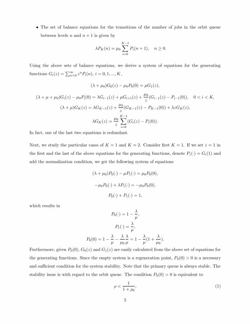
We denote the steady state probabilities for this system by Pi(n), i = 0, 1, ...,K, n = 0, 1, ..., where
the index i corresponds to the number of jobs in the primary queue and the index n corresponds
to the number of jobs in the orbit queue. Also, we denote the input rate to the system by λ, the
service rate of the primary queue by µ and the service rate of the orbit queue by µ0. We can write
the following sets of balance equations.
• For i = 0:
λP0(0) = µP1(0),
(λ + µ0)P0(n) = µP1(n), n ≥ 1,
• For 0 < i < K:
(λ + µ)Pi(0) = λPi−1(0) + µPi+1(0) + µ0Pi−1(1),
(λ + µ + µ0)Pi(n) = λPi−1(n) + µPi+1(n) + µ0Pi−1(n + 1), n ≥ 1,
• For i = K:
(λ + µ)PK(0) = λPK−1(0) + µ0PK−1(1),
(λ + µ)PK(n) = λPK−1(n) + µ0PK−1(n + 1) + λPK(n − 1), n ≥ 1,
4
• The set of balance equations for the transitions of the number of jobs in the orbit queue
between levels n and n + 1 is given by
λPK(n) = µ0
K−1∑
i=0
Pi(n + 1), n ≥ 0.
Using the above sets of balance equations, we derive a system of equations for the generating
functions Gi(z) =∑∞
n=0 znPi(n), i = 0, 1, ...,K,
(λ + µ0)G0(z) − µ0P0(0) = µG1(z),
(λ + µ + µ0)Gi(z) − µ0Pi(0) = λGi−1(z) + µGi+1(z) +µ0
z(Gi−1(z) − Pi−1(0)), 0 < i < K,
(λ + µ)GK(z) = λGK−1(z) +µ0
z(GK−1(z) − PK−1(0)) + λzGK(z),
λGK(z) =µ0
z
K−1∑
i=0
(Gi(z) − Pi(0)).
In fact, one of the last two equations is redundant.
Next, we study the particular cases of K = 1 and K = 2. Consider first K = 1. If we set z = 1 in
the first and the last of the above equations for the generating functions, denote Pi(·) = Gi(1) and
add the normalization condition, we get the following system of equations
(λ + µ0)P0(·) − µP1(·) = µ0P0(0),
−µ0P0(·) + λP1(·) = −µ0P0(0),
P0(·) + P1(·) = 1,
which results in
P0(·) = 1 − λ
µ,
P1(·) =λ
µ,
P0(0) = 1 − λ
µ− λ
µ0
λ
µ= 1 − λ
µ(1 +
λ
µ0).
Furthermore, given P0(0), G0(z) and G1(z) are easily calculated from the above set of equations for
the generating functions. Since the empty system is a regeneration point, P0(0) > 0 is a necessary
and sufficient condition for the system stability. Note that the primary queue is always stable. The
stability issue is with regard to the orbit queue. The condition P0(0) > 0 is equivalent to
ρ <1
1 + ρ0, (1)
5
with ρ = λ/µ and ρ0 = λ/µ0. That is, λ < (√
µ0(µ0 + 4µ) − µ0)/2. One can see that the stability
condition for the system composed of M/M/1/1 retrial queue and M/M/1/∞ orbit queue is more
restrictive than the stability condition for the classical queue with infinite buffer. We also note that
as µ0 → ∞, ρ0 → 0, and the above stability condition becomes the standard condition ρ < 1.
Next, let us analyze the case K = 2. Using again the equations for the generating functions and
setting z = 1, we obtain the following system of linear equations for P0(·), P1(·), P2(·), P0(0) and
P1(0)
(λ + µ0)P0(·) − µ0P0(0) = µP1(·),
(λ + µ + µ0)P1(·) − µ0P1(0) = λP0(·) + µP2(·) + µ0(P0(·) − P0(0)),
λP2(·) = µ0(P0(·) − P0(0)) + µ0(P1(·) − P1(0)),
λP0(0) = µP1(0),
P0(·) + P1(·) + P2(·) = 1.
The solution of the above system is given by
P0(·) = 1 − λ
µ,
P1(·) =λµ(µ + µ0) − λ2(µ0 − µ) − λ3
µ2(2λ + µ + µ0),
P2(·) =λ2(λ + µ + µ0)
µ2(2λ + µ + µ0),
P0(0) =µµ0(µ + µ0) − λµ0(µ0 − µ) − 2λ2µ0 − λ3
µµ0(2λ + µ + µ0),
P1(0) =λµµ0(µ + µ0) − λ2µ0(µ0 − µ) − 2λ3µ0 − λ4
µ2µ0(2λ + µ + µ0).
As in the case K = 1, the stability condition is given by
P0(0) > 0,
which is equivalent to
µµ0(µ + µ0) − λµ0(µ0 − µ) − 2λ2µ0 − λ3 > 0.
Sunstituting into the above inequality µ = λ/ρ and µ0 = λ/ρ0, we obtain the stability condition in
terms of ρ and ρ0 as follows:
−(1 + ρ0)2ρ2 + (1 + ρ0)ρ + ρ0 > 0. (2)
6
Solving the above quadratic inequality, we get
ρ <1 +
√1 + 4ρ0
2(1 + ρ0). (3)
Since 1 +√
1 + 4ρ0 > 2, the above condition (3) gives a larger region of stability than the one in
condition (1). As one could expect, the increase of the buffer space in the primary queue improves
the stability of the system. In the case of fast retransmissions (ρ0 → 0), condition (1) can be
approximated as
ρ < 1 − ρ0 + o(ρ0),
and condition (3) can be approximated as
ρ < 1 − ρ20 + o(ρ2
0).
In Figure 2 we plot the values of the right hand sides of conditions (1) and (3) for small and medium
values of ρ0. Clearly, the stability region increases significantly when moving from K = 1 to K = 2.
0 1 2 3 4 5 6 7 8 9 100
0.1
0.2
0.3
0.4
0.5
0.6
0.7
0.8
0.9
1
ρ0
K=1K=2
Figure 2: Comparison of stability conditions for K = 1 and K = 2 (right hand sides of inequalities
(1) and (3)).
Next, let us derive the stability condition for arbitrary K. Let us enumerate the system states (n, i)
in lexicographic order. Then, the Markov chain generator for the system has the block structure
7
Q = {Qij}i,j≥0 where
Qi,i−1 =
0 µ0 0 · · · 0 0
0 0 µ0 · · · 0 0
0 0 0 · · · 0 0...
......
. . ....
...
0 0 0 · · · 0 µ0
0 0 0 · · · 0 0
, i ≥ 1,
Qi,i =
−λ − (1 − δi,0)µ0 λ 0 · · · 0 0
µ −λ − µ − (1 − δi,0)µ0 λ · · · 0 0
0 µ −λ − µ − (1 − δi,0)µ0 · · · 0 0...
......
. . ....
...
0 0 0 · · · −λ − µ − (1 − δi,0)µ0 λ
0 0 0 · · · µ −µ
,
i ≥ 0,
Qi,i+1 =
0 0 0 · · · 0 0
0 0 0 · · · 0 0
0 0 0 · · · 0 0...
......
. . ....
...
0 0 0 · · · 0 0
0 0 0 · · · 0 λ
, i ≥ 0,
and the other blocks are zeros. All blocks are of dimension (K + 1) × (K + 1). Let us denote
Q0 = Qi,i−1, Q1 = Qi,i, and Q2 = Qi,i+1 for i ≥ 1. Then, the necessary and sufficient condition for
the system stability is given by the following inequalilty [4, 13]
xQ2e < xQ0e, (4)
where x is an 1 × (K + 1) vector which is the unique solution to the system
x(Q0 + Q1 + Q2) = 0,
xe = 1,(5)
and where e is the vector of ones and its dimension is (K + 1) × 1. The system (5) has an explicit
solution
xr = x0
(
λ + µ0
µ
)r
= x0ρr
(
1 + ρ0
ρ0
)r
, r = 0, ...,K, (6)
8
with
x0 =
(
K∑
r=0
(
λ + µ0
µ
)r)−1
.
Substituting (6) into (4), we obtain the following stability condition in terms of ρ and ρ0.
Proposition 1 The M/M/1/K retrial queue with M/M/1/∞ orbit queue is stable if and only if
1 +
K−1∑
r=1
ρr
(
1 + ρ0
ρ0
)r
− ρ0ρK
(
1 + ρ0
ρ0
)K
> 0. (7)
First, we note that the conditions (1) and (2) are indeed particular cases of the above general
condition (7). Then, let us study the limiting case K → ∞. Denote ξ = ρ 1+ρ0
ρ0. Using this new
notation, the condition (7) can be rewritten as follows:
1 +
K−1∑
r=1
ξr − ρ0ξK > 0,
or, equivalently,ξK − 1
ξ − 1− ρ0ξ
K > 0. (8)
Next, consider two cases 0 < ξ < 1 and ξ > 1. We note that the conditions 0 < ξ < 1 and ξ > 1 are
equivalent to the conditions ρ < ρ0
1+ρ0and ρ > ρ0
1+ρ0, respectively. When 0 < ξ < 1, the condition
(8) is equivalent to
ξK − 1 − ρ0ξK(ξ − 1) < 0.
Since 0 < ξ < 1, one can always find a sufficiently large K such that the above condition is satisfied.
Thus, the system is always stable in the case ρ < ρ0
1+ρ0. In the second case ξ > 1, the condition (8)
is equivalent to
ξK − 1 − ρ0ξK(ξ − 1) > 0.
We can rewrite the above condition as follows:
(1 + ρ0) − ρ0ξ −1
ξK> 0.
For the limiting case K → ∞, the above condition reduces to
ξ <1 + ρ0
ρ0.
or, equivalently,
ρ < 1.
9
Since ρ0
1+ρ0< 1, we can combine the two separate cases 0 < ξ < 1 and ξ > 1 to produce a single
stability condition: ρ < 1. This condition is expected as in the system with large buffer size K the
retrials are seldom and the system behaves similarly to the standard M/M/1 queue.
Now let us consider an approximate model where we assume that packets are dropped with a fixed
probability P . It was shown in [3] that the approximate model with fixed probabilities approximates
well the exact retrial model when the nominal load is small. First, we consider the case of arbitrary
value of K and then we study in more detail the cases K = 1 and K = 2.
Taking into account retransmissions, the actual load on the primary queue is given by the following
formula
ρ =ρ
1 − P, (9)
where ρ = λ/µ is the nominal load.
Assuming that the packets arrive to the primary queue according to a Poisson process, one can
use for the approximation the classical M/M/1/K queueing model. Thus, the drop probability is
given by
P =ρK(1 − ρ)
(1 − ρK+1), (10)
where K is the total buffer size in packets.
Proposition 2 If ρ < 1, the system of equations (9) and (10) has a unique solution. This solution
can be found by fixed point iterations
ρ(n+1) = ρ1 − (ρ(n))K+1
1 − (ρ(n))K(11)
which converges for any initial value ρ(0) ∈ [0,∞).
Proof: We substitute the expression for the packet loss probability (10) into (9) to get
ρ =ρ(1 − ρK+1)
1 − ρK.
We can rewrite it as follows:ρ(1 − ρK)
1 − ρK+1= ρ,
ρ + ρ2 + ... + ρK
1 + ρ + ρ2 + ... + ρK= ρ,
10
1 − 1
1 + ρ + ρ2 + ... + ρK= ρ.
Now let us consider the left hand side of the above equation. Clearly this function of ρ is strictly
increasing on the interval [0,∞). Moreover, it has a horizontal asymptote y = 1. Hence, if ρ ≥ 1,
there is no solution and if ρ < 1 there is a unique solution.
Next we show that the fixed point iterations (11) converge to the solution of (9) and (10). Since
the above considerations demonstrate that there is a unique fixed point (of course, we are now
interested only in the case ρ < 1), we only need to prove that the fixed point iterations converge.
To prove this, it is enough to show that the derivative of the right hand side of (11) is less than
one.d
dρ
[
ρ1 − ρK+1
1 − ρK
]
=d
dρ
[
ρ
(
1 +ρK
1 + ρ + ... + ρK−1
)]
=
ρKρK−1 + (K − 1)ρK + ... + 2ρ2K−3 + ρ2K−2
(1 + ρ + ... + ρK−1)2=
ρKρK−1 + (K − 1)ρK + ... + 2ρ2K−3 + ρ2K−2
1 + 2ρ + ... + KρK−1 + (K − 1)ρK + ... + 2ρ2K−3 + ρ2K−2< ρ < 1
This completes the proof.
2
Let us now consider the particular case K = 1. Solving the system of fixed point equations
P =ρ
1 + ρ,
ρ =ρ
1 − P,
we obtain
P = ρ,
ρ =ρ
1 − ρ.
Now recall that in the case K = 1 we have P1(·) = ρ. Hence, in this particular case the approximate
packet drop probability P matches exactly P1(·).
Next, we consider the particular case K = 2. By solving the set of fixed point approximation
equations
P =ρ2
1 + ρ + ρ2,
ρ =ρ
1 − P,
11
we obtain
P =1
4(√
1 + 3ρ −√
1 − ρ)2.
First, we note that in contrast to the case K = 1 the approximate packet drop probability P does
not match exactly P2(·). There are two important limiting cases:
P2(·) =λ2(λ + µ + µ0)
µ2(2λ + µ + µ0)→ ρ2, as µ0 → ∞,
P2(·) =λ2(λ + µ + µ0)
µ2(2λ + µ + µ0)→ ρ2(1 + ρ)
1 + 2ρ, as µ0 → 0.
In Figures 3 and 4 we plot the relative error |P − P2(·)|/P2(·) as a function of ρ for the limiting
cases µ0 → ∞ and µ0 → 0, respectively.
0 0.1 0.2 0.3 0.4 0.5 0.6 0.7 0.8 0.9 10
0.05
0.1
0.15
0.2
0.25
ρ
Figure 3: The relative error |P − P2(·)|/P2(·) in the limiting case µ0 → ∞.
As one can see, P approximates P2(·) well when ρ and µ0 are both small.
3 Two M/M/1/1 queues in tandem with M/M/1/∞ ordit queue
As another particular case of the network of finite queues with retrials, let us consider two M/M/1/1
queues in tandem with M/M/1/∞ orbit queue. We denote the steady state probabilities for this
system by Pij(n), i, j = 0, 1 and n = 0, 1, ... , where the indicies i and j correspond to the number
12
0 0.1 0.2 0.3 0.4 0.5 0.6 0.7 0.8 0.9 10
0.2
0.4
0.6
ρ
Figure 4: The relative error |P − P2(·)|/P2(·) in the limiting case µ0 → 0.
of jobs in the first and the second queues, respectively, and n corresponds to the number of jobs in
the ordit queue. We denote the input rate to the system by λ, the service rate of queue k by µk,
k = 1, 2, and the service rate of the orbit queue by µ0. The transition rate diagram is depicted in
Figure 5. We can write the following five sets of balance equations:
• For the (0, 0) column:
λP00(0) = µ2P01(0), (12)
(λ + µ0)P00(n) = µ2P01(n), n ≥ 1,
• For the (1, 0) column:
(λ + µ1)P10(0) = λP00(0) + µ0P00(1) + µ2P11(0),
(λ + µ1)P10(n) = λP00(n) + µ0P00(n + 1)λP10(n − 1) + µ2P11(0), n ≥ 1,
• For the (0, 1) column:
(λ + µ2)P01(0) = µ1P10(0),
(λ + µ2 + µ0)P01(n) = µ1P10(n) + µ1P11(n − 1), n ≥ 1,
13
• For the (1, 1) column:
(λ + µ1 + µ2)P11(0) = λP01(0) + µ0P01(1),
(λ + µ1 + µ2)P11(n) = λP01(n) + µ0P01(n + 1) + λP11(n − 1), n ≥ 1,
• Taking a “cut” between levels n and n + 1 of the number of jobs in orbit yields:
λP10(n) + (λ + µ1)P11(n) = µ0P00(n + 1) + µ0P01(n + 1), n ≥ 0.
λ λ
λ
λ
λ
λ
λ
λ
λ
λ
λ
λ
µ
µ
µ
µ
µ
µµ
µ µµ
µ
µ
µ
µ
µ
µ
1
2
1
1
0
2
21
2
1
1
00
0
2
2
(1,0) (1,1)
0
1
2
(0,0) (0,1)
Figure 5: Transition rate diagram
Using the above sets of balance equations, we derive a system of equations for the generating
functions Gij(z) =∑∞
n=0 znPij(n), i, j = 0, 1.
(λ + µ0)G00(z) − µ2G01(z) = µ0P00(0), (13)
(λz + µ0)G00(z) − z(λ(1 − z) + µ1)G10(z) + µ2zG11(z) = µ0P00(0), (14)
−µ1G10(z) + (λ + µ2 + µ0)G01(z) − µ1zG11(z) = µ0P01(0), (15)
(λz + µ0)G01(z) − z(λ(1 − z) + µ1 + µ2)G11(z) = µ0P01(0), (16)
µ0G00(z) − λzG10(z) + µ0G01(z) − (λ + µ1)zG11(z) = µ0P00(0) + µ0P01(0). (17)
14
Next, we denote Pij(·) = Gij(1) for i, j = 0, 1, and set z = 1 in equations (13),(14),(15),(17), add
equation (12) and the normalization equation P00(·) + P10(·) + P01(·) + P11(·) = 1. This results in
a system of linear independent equations:
(λ + µ0)P00(·) − µ2P01(·) = µ0P00(0),
(λ + µ0)P00(·) − µ1P10(·) + µ2P11(·) = µ0P00(0),
−µ1P10(·) + (λ + µ2 + µ0)P01(·) − µ1P11(·) = µ0P01(0),
µ0P00(·) − λP10(·) + µ0P01(·) − (λ + µ1)P11(·) = µ0P00(0) + µ0P01(0),
λP00(0) = µ2P01(0),
P00(·) + P10(·) + P01(·) + P11(·) = 1.
The solution of the above system of linear equations leads to the following result
Proposition 3 The probabilities Pij(·) and Pij(0) for i, j = 0, 1 are given by
P00(·) = 1 − λ
µ1− λ
µ2,
P10(·) =λ
µ1,
in particular, implying that
P01(·) + P11(·) =λ
µ2,
P01(·) =λ(µ1µ2(µ1 + µ2 + µ0) − λ(µ0(µ1 + µ2) − µ1µ2) − λ2(µ1 + µ2))
µ1µ22(2λ + µ1 + µ2 + µ0)
,
P11(·) =λ2(λ(µ1 + µ2) + µ0(µ1 + µ2) + µ1µ2)
µ1µ22(2λ + µ1 + µ2 + µ0)
,
P00(0) =1
µ0µ1µ2(2λ + µ1 + µ2 + µ0)
(
µ0µ1µ2(µ1 + µ2 + µ0) − λ[µ20(µ1 + µ2) + µ0(µ
21 + µ2
2)]
−λ2[µ21 + µ2
2 + µ1µ2 + 2µ0(µ1 + µ2)] − λ3[µ1 + µ2])
,
P01(0) =λ
µ2P00(0),
P10(0) =λ(λ + µ2)
µ1µ2P00(0),
P11(0) =λ2(λ2 + λ(µ1 + µ2 + µ0) + µ0(µ1 + µ2) + µ1µ2)
µ1µ22(2λ + µ1 + µ2 + µ0)
P00(0).
15
Again, as in the case of a single M/M/1/1 retrial queue, once P00(0) and P01(0) are determined, the
generating functions Gij(z) are uniquely determined by the system of linear equations (13)-(16).
Let us now investigate the stability of the system. We argue that the empty system is a regeneration
point, and hence P00(0) > 0 is a necessary and sufficient condition for the system stability. The
condition P00(0) > 0 is equivalent to
µ0µ1µ2(µ1 + µ2 + µ0) − λ[µ20(µ1 + µ2) + µ0(µ
21 + µ2
2)]
−λ2[µ21 + µ2
2 + µ1µ2 + 2µ0(µ1 + µ2)] − λ3[µ1 + µ2] > 0. (18)
As the above expression seems to be too complex to analyse in the general case, we consider two
important particular cases: the case of large µ0 and the case of µ1 = µ2.
We note that for large values of µ0 the probability P00(0) has a simple asymptotics. Namely, we
have
P00(0) → 1 − λ
µ1− λ
µ2,
as µ0 → ∞. Thus, ifλ
µ1+
λ
µ2< 1, (19)
then there always exists a large enough value of µ0 that ensures the stability of the system.
Next, let us consider the case µ1 = µ2 =: µ. Without loss of generality, we can take λ = 1. The
stability condition (18) becomes
(µ − 2)µ20 + 2[µ(µ − 1) − 2]µ0 − 3µ − 2 > 0. (20)
We first note that if µ < 2, then µ − 2 < 0 and µ(µ − 1) − 2 < 0, and consequently, the stability
condition cannot be satisfied by any choice of µ0. Thus, a necessary condition for stabililty in this
particular case is µ > 2. Once this condition is guaranteed, the parameter µ0 has to be chosen
greater than the positive root of the left hand side of (20). Namely,
µ0 >
√
µ3(µ − 2) − [µ(µ − 1) − 2]
µ − 2.
We note that the right hand side of the above inequality has the asymptotics 3/(2µ) as µ → ∞.
Indeed, when µ becomes very large, (almost) every job passes through queues 1 and 2 without
blocking. If there are a few jobs that get blocked, a (very) small value of µ0 > 3/(2µ) will ensure
stability.
16
Next, let us analyze the fixed point approximation model which is described by the following set
of equations
ρ1 =ρ1
(1 − P1)(1 − P2), (21)
ρ2 =ρ2
(1 − P2), (22)
P1 =ρ1
1 + ρ1, (23)
P2 =ρ2
1 + ρ2. (24)
Note that equations (22) and (24) correspond exactly to the single node case with K = 1. Hence,
we have
P2 = ρ2,
and
ρ2 =ρ2
1 − ρ2.
Then, to get P1 and ρ1, we substitute P2 = ρ2 and P1 from equation (23) into equation (21),
ρ1 =ρ1
(1 − P1)(1 − ρ2), (25)
which results in
ρ1 =ρ1
1 − ρ1 − ρ2,
and, consequently, we have
P1 =ρ1
1 − ρ2.
Note that the system of equations (21)-(24) has a unique and positive solution if and only if
ρ1 + ρ2 < 1. It is interesting that this condition coincides with the stability condition (19) for the
limiting case when µ0 → ∞.
Let us now study the average number of jobs in the system. Differentiating equations (13),(14),(15),
and (17), then setting z = 1 and denoting Lij := G′ij(1), i, j = 0, 1, we obtain a system of linear
equations
(λ + µ0)L00 − µ2L01 = 0, (26)
(λ + µ0)L00 − µ1L10 + µ2L11 = −λP00(·) − (λ − µ1)P10(·) − µ2P11(·), (27)
−µ1L10 + (λ + µ2 + µ0)L01 − µ1L11 = µ1P11(·), (28)
µ0L00 − λL10 + µ0L01 − (λ + µ1)L11 = λP10(·) + (λ + µ1)P11(·). (29)
17
Proposition 4 The average number of jobs in orbit is given by
Lorbit = L00 + L10 + L01 + L11, (30)
the average number of jobs in the system is given by
Lsystem = Lorbit + P10(·) + P01(·) + 2P11(·), (31)
and the average time spent by a job in the system is given by
Tsystem = Lsystem/λ, (32)
where Lij, i, j = 0, 1 are provided by the solution of the system of equations (26)-(29), and the
probabilities Pij(·) are given in Proposition 3. Moreover, denoting by L1 and L2 the mean queue
size in the first and the second M/M/1/1 queues, respectively, we have
L1 = P10(·) + P11(·),
L2 = P01(·) + P11(·),
and
Lsystem = Lorbit + L1 + L2.
Let us consider a numerical example. We fix λ = 1 and the total network capacity µ1 + µ2 = 5.
In Figure 6, we plot the average number of jobs in the system Lsystem as a function of the first
node capacity µ1. We study two cases: µ0 = 4 and µ0 = 7. First, we observe that in the middle of
the capacity value range, the value of Lsystem becomes less sensitive when µ0 increases. Second, it
seems that the minimal value of Lsystem is achieved when µ1 = µ2. This fact is further confirmed
by the more detailed Figure 7, but, of course, requires additional analytic investigation.
Acknowledgements
We would like to thank A.N. Dudin and V.I. Klimenok for drawing our attention to the necessary
and sufficient condition for stability of quasi-Toeplitz Markov chains. We also would like to ac-
knowledge the support of the EuroNGI Network of Exellence and the France Telecom R&D (Grant
“Modelisation et Gestion du Trafic Reseaux Internet” no. 42937433).
18
1.8 2 2.2 2.4 2.6 2.8 3 3.20
10
20
30
40
50
60
70
80
capacity of the first node
aver
age
num
ber
of jo
bs
µ0=4.0
µ0=7.0
Figure 6: Lsystem as a function of µ1 given µ1 + µ2 = 5
References
[1] Allman, M., Paxson, V., & Stevens, W. (1999). TCP congestion control. RFC 2581. Available
at http://www.ietf.org/rfc/rfc2581.txt.
[2] Artalejo, J.R. (1999). Accessible bibliography on retrial queues, Mathematical and computer
modelling 30: 223–233.
[3] Cohen, J.W. (1957). Basic problems of telephone traffic theory and the influence of repeated
calls. Philips Telecommunication Review 18: 49–100.
[4] Dudin, A.N., & Klimenok, V.I. (1999). Multi-dimensional quasi-Toeplitz Markov chains. Jour-
nal of Applied Mathematics and Stochastic Analysis, 12: 393–415.
[5] Falin, G.I. (1990). A survey of retrial queues. Queueing Systems, 7: 127–167.
[6] Falin G.I. & Templeton, J.G.C. (1997). Retrial queues, CRC Press.
[7] Floyd S. & Jacobson V. (1993). Random early detection gateways for congestion avoidance.
IEEE/ACM Transactions on Networking 1: 397–413.
19
2.48 2.485 2.49 2.495 2.5 2.505 2.51 2.515 2.526.2
6.201
6.202
6.203
6.204
6.205
capacity of the first node
aver
age
num
ber
of jo
bs
Figure 7: Lsystem as a function of µ1 given µ1 + µ2 = 5 (detailed plot for µ0 = 4.0).
[8] Jacobson, V. (1988). Congestion avoidance and control. In Proceedings of ACM SIGCOMM’88,
pp. 314–329.
[9] Kelly, F.P., Maulloo, A., & Tan, D. (1998). Rate control for communication networks: shadow
prices, proportional fairness and stability. Journal of Operational Research Society, 49: 237–
252.
[10] Kim, C.S., Klimenok, V.I., & Orlovsky, D.S. (2004). The BMAP/PH/N/N + R retrial queu-
ing system with different disciplines of retrials. In Proceedings of ASMTA’04, Magdeburg,
Germany.
[11] Kunniyur, S., & Srikant, R. (2000). End-to-end congestion control schemes: utility functions,
random losses, ECN marks. In Proceedings of IEEE INFOCOM’00. An extended version has
appeared in IEEE/ACM Transactions on Networking 11:689–702, 2003.
[12] Low, S.H., & Lapsley, D.E. (1999). Optimization flow control I: Basic algorithm and conver-
gence. IEEE/ACM Transactions on Networking 7:861–874.
[13] Neuts, M. (1989). Structured stochastic matrices of M/G/1 type and their applications, Marcel
Dekker, New York.
20