Retrieval of Model Grid-Scale Heat Capacity Using...

Retrieval of Model Grid-Scale Heat Capacity Using Geostationary Satellite Products.Part I: First Case-Study Application

RICHARD T. MCNIDER

Department of Atmospheric Science, University of Alabama in Huntsville, Huntsville, Alabama

WILLIAM M. LAPENTA

NASA Marshall Space Flight Center, Huntsville, Alabama

ARASTOO P. BIAZAR

Department of Atmospheric Science, University of Alabama in Huntsville, Huntsville, Alabama

GARY J. JEDLOVEC AND RONNIE J. SUGGS

NASA Marshall Space Flight Center, Huntsville, Alabama

JONATHAN PLEIM

Atmospheric Science Modeling Division, National Oceanic and Atmospheric Administration/Air Resources Laboratory, ResearchTriangle Park, North Carolina

(Manuscript received 12 August 2004, in final form 22 February 2005)

ABSTRACT

In weather forecast and general circulation models the behavior of the atmospheric boundary layer,especially the nocturnal boundary layer, can be critically dependent on the magnitude of the effective modelgrid-scale bulk heat capacity. Yet, this model parameter is uncertain both in its value and in its conceptualmeaning for a model grid in heterogeneous conditions. Current methods for estimating the grid-scale heatcapacity involve the areal/volume weighting of heat capacity (resistance) of various, often ill-defined,components. This can lead to errors in model performance in certain parameter spaces. Here, a techniqueis proposed and tested for recovering bulk heat capacity using time tendencies in satellite-retrieved surfaceskin temperature (SST). The technique builds upon sensitivity studies that show that surface temperatureis most sensitive to thermal inertia in the early evening hours. The retrievals are made within the contextof a surface energy budget in a regional-scale model [the fifth-generation Pennsylvania State University–National Center for Atmospheric Research Mesoscale Model (MM5)]. The retrieved heat capacities areused in the forecast model, and it is shown that the model predictions of temperature are improved in thenighttime during the forecast periods.

1. Introduction

The behavior of the nocturnal boundary layer is criti-cal to operational weather forecasts of minimum tem-peratures and winds related to agricultural freeze warn-

ings, utility load forecasting, transportation fog adviso-ries, and other interests. Additionally, air pollutionexposure from surface sources is often highest in stableconditions as a result of a lack of ventilation and ver-tical mixing. Ironically, long-term exposure of humansand plants to certain air pollutants, such as ozone, canoccur when the nocturnal boundary layer fails to stabi-lize, allowing the continued downward flux of ozonefrom the residual boundary layer above. The behaviorof the atmospheric boundary layer, especially the noc-

Corresponding author address: Dr. Richard T. McNider, Na-tional Space Science and Technology Center, 320 SparkmanDrive, Huntsville, AL 35605.E-mail: [email protected]

1346 J O U R N A L O F A P P L I E D M E T E O R O L O G Y VOLUME 44

© 2005 American Meteorological Society

JAM2270

turnal boundary, is critically dependent on the surfaceheat capacity, or, more generally, a surface resistanceparameter.

In the following, a technique for recovering an effec-tive grid-scale heat capacity or resistance parameter us-ing evening skin temperature time tendencies from geo-stationary satellites is described. The use of the morn-ingtime tendencies of air (Mahfouf 1991) and skin(McNider et al. 1994, hereinafter McN94; Norman et al.1995) temperatures has been employed to recover in-formation relative to surface moisture. However, theuse of evening skin tendencies for retrieving informa-tion on the surface heat capacity or resistance has notbeen reported. The recovery of soil moisture and therecovery of heat capacity, as presented here, have com-mon attributes in that both are based on the modelsensitivity studies of Carlson (1986) and Wetzel et al.(1984). These show (for reasonable parameter spaces)that the morning rise in surface temperature is mostdependent on surface moisture, whereas the eveningtendencies are most sensitive to thermal inertia. In bothcases the sensitivity assessment assumes that most ofthe error in a modeled skin tendency is the result oferrors in the specification of the most sensitive variable.Both techniques are similar in that they also assumethat other terms in the surface heat balance are correct.This is an assumption that can fail. McN94 used specialobservations from the First International Satellite LandSurface Climatology Project (ISLSCP) Field Experi-ment (FIFE) and Mahfouf (1991) from the Hydrologi-cal Atmospheric Pilot Experiment–Modélisation du Bi-lan Hydrique (HAPEX–MOBILHY) to evaluate theother terms in the equations.

Here, initial tests of recovering the heat capacity arepresented. While the results of these tests are encour-aging in that the use of the recovered heat capacityimproved model predictions of the nocturnal boundarylayer, the general application of this technique mayhave to be limited to certain synoptic situations. In asecond part of this paper (R. T. McNider et al. 2005,unpublished manuscript, hereinafter Part II), the be-havior of the stable boundary layer is explored, and thisanalysis shows that the recovery of the heat capacitymay, in practice, be limited to certain parameter spaces.Additionally, it addresses the day-to-day consistency ofthe retrieved heat capacities and issues with sensitivityand numerical solution techniques.

2. Background on the heat capacity parameter

Before discussing the satellite assimilation strategies,we review surface energy budget formulations and, spe-cifically, the role of surface heat capacity in weather

forecast and global climate models. Most early meso-scale models (Mahrer and Pielke 1976; Physick 1976;McNider and Pielke 1981) utilized a heat balance equa-tion at the surface of the following form:

0 � RN � H � G � E, �1�

where RN is the net radiation (including net shortwave,incoming atmospheric longwave, and outgoing long-wave), H is the sensible heat flux, G is the soil heat flux,and E is the latent heat flux. The surface was repre-sented as an infinitesimally small layer with zero heatcapacity. Temperature was calculated through root-finding techniques, and heat capacity was not relevantin the flux to this infinitesimal surface because heatcapacity has no meaning for a zero mass surface andcancels in the definition of the ground heat flux,

G � Cg��TS��z � Cg

�

Cg�TS��z. �2�

Here, TS is the soil temperature, Cg is the soil volumet-ric heat capacity (soil density times specific heat capac-ity), � is the soil thermal conductivity, and �, whichcombines heat capacity and conductivity, is referred toas the soil diffusivity (McCumber and Pielke 1981; Pe-ters-Lidard et al. 1998). Note that this equation neglectsadvection and normally assumes vertical homogeneityin the soil. The heat capacity is relevant to the localchange of temperature in the soil

�TS

�t�

�

Cg�TS��z, �3�

potentially impacting G by affecting the surface gradi-ent �TS /�Z. McCumber and Pielke (1981) also consid-ered that the heat capacity and diffusivity should in-clude dependence on soil moisture.

Other early models (Blackadar 1979; Bhumralkar1975) used a prognostic equation for the surface tem-perature of the form

Cb��TG

�t � � RN � H � G � E, �4�

where TG is the surface temperature. This form nowincludes what is referred to as a storage term Cb�TG/�t,because it represents the imbalance in the forcing termson the right-hand side. The definition and interpreta-tion of Cb depends on what the surface includes.Blackadar (1979) took the surface to be a uniform slabthat is representative of bare soil. Thus, Cb representedthe heat capacity over some assumed depth of the slab,that is, Cb � Cg � dS. Blackadar also specified Cb suchthat it included the diurnal frequency and conductiv-ity so that the single-layer slab model would replicate

SEPTEMBER 2005 M C N I D E R E T A L . 1347

the phase and amplitude of the surface temperaturefrom that of a multilayer, analytical soil model. Thus,for the slab model, the depth dS, as a scaling parameter,enters through the conductivity and thermal forcing fre-quency so that

Cb � ��Cg

2� �1�2

. �5�

Here it can be seen that Cb involves both volumetricheat capacity and thermal conductivity, and is some-times referred to as the heat capacity per unit area ofthe slab, or what we will refer to as bulk heat capacity(Pleim and Xiu 1995). This is the basic form of theforce–restore model that is implemented in the fifth-generation Pennsylvania State University–NationalCenter for Atmospheric Research Mesoscale Model(MM5), described by Grell at al. (1994).

In a similar context of an analytical model, Carlson etal. (1981) defined the thermal inertia ,

� � ��Cg�1�2, �6�

as a key parameter in the response of the surface toenergy inputs. Other investigators, such as Wetzel andChang (1988), examining fluxes over vegetative cano-pies, considered that the surface might include vegeta-tion or standing water, such as dew. They suggestedthat Cb represented a vegetation-layer capacity that isdetermined as the biomass fraction times the heat ca-pacity of water plus the dew. Thus,

Cb � �bm � WR�CW, �7�

where bm is the water-equivalent biomass fraction, WR

is the water or dew on the vegetation, and CW is theheat capacity of water (Argentini et al. 1992).

Smirnova et al. (1997) provided an interface-spanning formulation that included both the soil and athin atmospheric layer. Then,

Cb � ��AcP�zA � Cg�zs�, �8�

where �A is the air density, �zA is the thin atmosphericlayer depth, and �zs is the first layer soil depth.

As investigators begin to apply the equations in mod-els where both bare soil and vegetation might bepresent (Noilhan and Planton 1989; Jacquemin andNoilhan 1990), the form of the equations was changedto write the heat capacity as a heat capacity coefficientCT, the inverse of the heat capacity parameter Cb,that is,

��TG

�t � � CT�RN � H � G � E�. �9�

The heat capacity coefficient was then usually deter-mined as a harmonic average of the heat capacities ofvegetation, soil, or other substances. For example, Noil-han and Planton (1989) used

CT � 1��1 veg

C̃bg

�veg

C̃b�. �10�

Here, C̃bg represents the heat capacity coefficientfor soil, and C̃b� represents the vegetation coefficient.1

Because the importance of the inclusion of soil mois-ture freezing has been established (Viterbo et al. 1999;Boone et al. 2000), more complicated forms have beenused, such as

CT � 1��1 veg��1 f�

C̃bg

��1 veg�f

C̃bi

�veg

C̃b�, �11�

by Giard and Bazile (2000), where f is the fraction offrozen water in the soil and C̃bi is the heat capacitycoefficient of ice.

The correct specification of the vegetative capacityhas been subject to debate as well as, perhaps, thespecification of CT in general. Pleim and Xiu (1995)argued that the value for vegetative heat capacity thatwas used by Noilhan and Planton (1989) (C̃b� � 10 3 Km2 J 1) was far too large for reasonable model perfor-mance. This was also indicated by Manzi and Planton(1994). Mahfouf et al. (1995) proposed C̃b� � 2 � 10 5

K m2 J 1. Giard and Bazile (2000) reduced this valueeven further to C̃b� � 8 � 10 6 K m2 J 1. (One has tobe careful when discussing large and small, reduce orincrease, because C̃b is the inverse of Cb.)

In fact, there has been substantial tuning of the CT

parameter based on model performance, with argu-ments for the tuning based on uncertainties in vegeta-tive canopy heat transfer. Even for bare soils the effectsof moisture and texture on heat capacity makes speci-fication difficult. For complex settings, such as mixedland uses that are encountered in general weather fore-casts and in GCMs, the specification of Cb or CT is farfrom being settled. In the following we will use the termbulk heat capacity to refer to this parameter, but intendthat its meaning is that of a combined heat capacity andheat transfer parameter, as given in Eqs. (10) or (11).

In examining Eqs. (1) or (6), it seems clear that be-cause Cb or CT is a direct multiplier of all of the flux

1 Here trying to put the notation across the literature in a com-mon form is difficult. We use � to indicate that the C̃b is 1/Cb sothat C̃b has units of inverse joules times meters squared timeskelvins, which is the inverse of the units of the heat capacityparameter Cb in Eq. (2) above.


terms, its magnitude should be critical to model theground temperature performance. Errors or uncer-tainty in the specification of CT of factors up to ordersof magnitude, as discussed above, are of considerableconcern in getting the right surface tendency and, ulti-mately, the right surface temperature in NWP modelsand GCMs. The error in specifying CT is at least aslarge as errors in the actual flux terms. One only has toimagine the real-world example of the eastern UnitedStates, which has mixed vegetation of different types,different soils and textures, rocks, roads, standing wa-ter, and so on, to recognize the difficulty in specifyingCB for a model grid. The following discusses a proposedtechnique for specifying the heat capacity/resistance pa-rameter using satellite data as an observational con-straint. Fundamentally, the technique uses the satelliteradiometer to measure the surface temperature changeover the model grid area to derive an improved effec-tive bulk heat capacity parameter. This is somewhatequivalent to the way in which a laboratory uses a ther-mometer to measure temperature change for a knowninput of energy to determine a heat capacity of somesubstance. In the present application, the “known” en-ergy input is not perfect because these are the fluxterms, but sensitivity analyses bolster the confidencethat more error may exist in the a priori specification ofCB than in the flux terms. The following outlines thetechnique.

3. Methodology

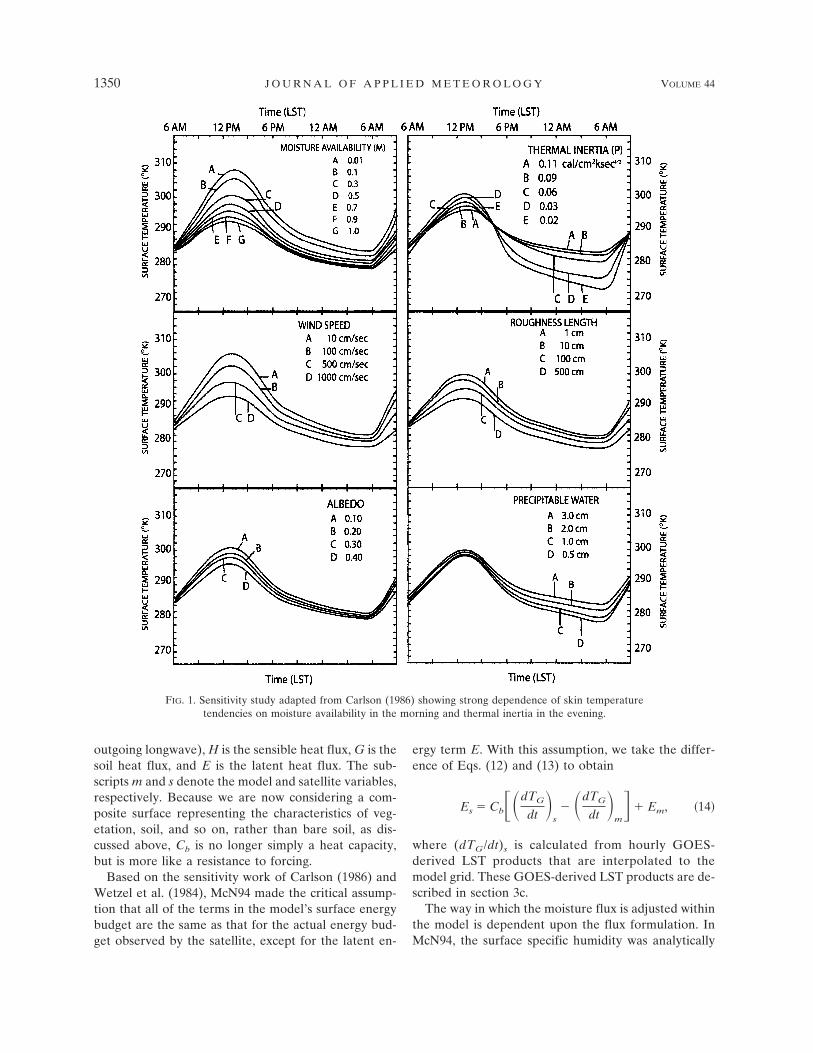
Carlson et al. (1981) and others have argued that thesurface energy terms with the largest uncertainty, interms of their impact on model sensitivity, are the ther-mal inertia (�Cg)1/2, defined above, and the surfacemoisture availability. Figure 1 from Carlson (1986)shows the sensitivity of a model to variations of the keymodel parameters. For the range of reasonable specifi-cation and uncertainty, the morning temperature ismost sensitive to moisture availability, and the eveningtemperature is most sensitive to thermal inertia. Otherfactors, such as roughness, and so on, showed less sen-sitivity for reasonable ranges of specification. For ex-ample, moisture availability might truly span the rangefrom near 0.0 to 1.0, but one would not expect the errorin roughness specification to span the range from 1 cmto 5 m. Carlson (1986), Price (1982), and others devel-oped techniques to use day and night passes of polar-orbiting IR sensors as two independent pieces of infor-mation to simultaneously recover thermal inertia andsurface moisture availability. The techniques showedpromise in case studies; however, the inversion processdid not always produce a unique solution. Further, sta-

tionary conditions over the 12-h passing time of thepolar orbiters that were required for the techniquewere not always met. Thus, while these techniques werepioneering, they have evidently not been widely used inthe initialization of operational NWP models or othermesoscale model applications.

To avoid some of the difficulty with the Carlson(1986) and Price (1982) polar-orbiter technique, Wetzelet al. (1984) proposed to use midmorning skin tempera-ture tendencies from geostationary satellites to recoverthe surface moisture availability. McN94, building uponthe work of Carlson, Price, and Wetzel et al., developeda technique to use morning skin temperatures tenden-cies from Geostationary Operational EnvironmentalSatellite (GOES) to recover soil moisture. Jones et al.(1998a,b) extended the work of McN94 by retrievingstomatal resistance. Lapenta et al. (1999) implementedthe technique within the MM5 system (Grell et al.1994), and the technique has undergone extensive test-ing in a semi-operational setting for weather forecastsand air pollution modeling applications. It has provedto decrease model bias and standard error of tempera-ture and humidity in long-term statistical tests (Lapentaet al. 1999). Diak and Whipple (1995) have also usedmorning tendencies for the specification of model pa-rameters to improve model performance.

We now turn our attention to the other term identi-fied by Carlson (1986), in addition to moisture avail-ability, that has large uncertainty, and yet to which thesurface cooling rate is sensitive—thermal inertia (andrelated heat capacity). As noted above, heat capacity isan extremely difficult quantity to specify based on tra-ditional land use data. The following describes the useof an observational constraint—evening skin tempera-tures from GOES—in a mesoscale model to recover thebulk grid-scale heat capacity.

a. Retrieval of bulk heat capacity using eveningskin tendencies

Following McN94, we first define the surface energybudget of the model for a composite surface (the mix-ture approach; Koster and Suarez 1992) as

Cbm�dTG

dt �m� �RN � H � G�m � Em �12�

and the energy budget observed by the satellite as

Cbs�dTG

dt �s� �RN � H � G�s � Es, �13�

where dTG/dt is the rate of change of the land surfacetemperature (LST), RN is the net radiation (includingnet shortwave, incoming atmospheric longwave, and


outgoing longwave), H is the sensible heat flux, G is thesoil heat flux, and E is the latent heat flux. The sub-scripts m and s denote the model and satellite variables,respectively. Because we are now considering a com-posite surface representing the characteristics of veg-etation, soil, and so on, rather than bare soil, as dis-cussed above, Cb is no longer simply a heat capacity,but is more like a resistance to forcing.

Based on the sensitivity work of Carlson (1986) andWetzel et al. (1984), McN94 made the critical assump-tion that all of the terms in the model’s surface energybudget are the same as that for the actual energy bud-get observed by the satellite, except for the latent en-

ergy term E. With this assumption, we take the differ-ence of Eqs. (12) and (13) to obtain

Es � Cb��dTG

dt �s �dTG

dt �m�� Em, �14�

where (dTG/dt)s is calculated from hourly GOES-derived LST products that are interpolated to themodel grid. These GOES-derived LST products are de-scribed in section 3c.

The way in which the moisture flux is adjusted withinthe model is dependent upon the flux formulation. InMcN94, the surface specific humidity was analytically

FIG. 1. Sensitivity study adapted from Carlson (1986) showing strong dependence of skin temperaturetendencies on moisture availability in the morning and thermal inertia in the evening.


recovered from similarity theory using this satellite-inferred evapotranspiration (Es). In MM5, surface spe-cific humidity is not a prognostic variable. Therefore,the moisture availability parameter was retrieved. Thisis also accomplished through inversion of surface simi-larity expressions (Lapenta et al. 1999).

Returning to the energy budgets as seen by themodel and satellite in Eqs. (8) and (9), respectively, wenow consider that the model Cbm may be different thanthe satellite Cbs. We will also employ the sensitivityresults of Carlson (1986) to make the assumption thatthe evening skin tendencies are most sensitive to ther-mal inertia (and related heat capacity). Carlson andothers have suggested that the balance in the nocturnalboundary layer is dominated by the longwave outgoingradiation from the surface and the flux of heat from theground flux. This balance is best realized under lightwinds and for simple bare-soil situations. Under suchconditions, or if we make the assumption that moistureavailability has been correctly specified (or is negli-gible, which may be largely true if stomata have closed),we can subtract Eqs. (12) and (13) to solve for Cbs. Weassume that there is negligible difference in net radia-tion, sensible heat flux, and soil heat flux. Thus,

Cbs � Cbm�dTG

dt �m��dTG

dt �s. �15�

The assumption made here about the soil heat flux be-ing specified correctly in the model is perhaps incon-gruous with the arguments above that the heat capacityor thermal inertia are not well known. However, forconvenience we make the assumption that all of theerror is initially in Cbm rather than in both Cbm and thesoil heat flux. As an alternative, because Cg is containedin the soil heat flux term Eq. (2) and in Cbm, one couldattempt to solve for Cg directly using both terms, al-though the inversion would be more difficult. However,for this first attempt we solve for Cbs and then changeCg using Eq. (3) in the heat flux terms.

The initial value for the model Cbm would be deter-mined in the normal fashion from land use information(see below). The new Cbs would be subsequently usedas the model value; thus, the new Cb does impact theground heat flux. We believe the natural averaging inthe satellite IR pixel is an advantage in the techniquedescribed below for recovering the composite surfacegrid-scale Cb. In carrying out the above retrieval, onehas to be especially careful that the satellite is actuallyseeing the surface to determine the skin temperaturetendencies. Cloud masks are more difficult to define inthe evening. Section 3c describes the satellite process-ing and methods for deducing the tendencies that areneeded in Eq. (15).

We recognize that the above characterization of thesurface energy budget in Eq. (12) is highly simplified,and that Cb contains multiple physical factors, such ascanopy mechanical and radiative exchange, soil andvegetative heat capacity, and so on. However, giventhat the actual surface is incredibly complicated anddoes not lend itself readily to a first-principle modeland the associated multiple parameters that would beinvolved, we believe that Cb as a model heuristic con-strained by observations has utility in many modelingendeavors.

b. Use and specification of bulk heat capacity inMM5

In the present study, we employ MM5 to recover thebulk heat capacity and, thus, as a preface give details ofhow heat capacity and thermal inertia are used andspecified in MM5. Based on the Blackadar (1979) ap-proach discussed above [see Eq. (3)], in MM5 Cb isrelated to thermal conductivity (�), heat capacity perunit volume (Cg), and the angular velocity of the earth() by

Cb � 0.95��Cg

2� �1�2

� 3.293 � 106��Cg�1�2

� 3.293 � 106�, �16�

where thermal inertia [ � (�Cg)1/2] is supplied (calcm 2 K 1 s 1/2).2 Except for the five-layer soil modelCb is used for all soil options within MM5. For thefive-layer soil model, volumetric heat capacity (Cg) isrecovered from thermal inertia and, subsequently, thebulk heat capacity (Cb) is obtained as

Cb � Cg � �z, �17�

where �z is the top soil-layer thickness (1 cm). FromEq. (4) thermal inertia () is related to thermal con-ductivity (�) and volumetric heat capacity and using thedefinition of diffusivity in Eq. (2),

� � �Cg. �18�

According to Dudhia (1996), � is chosen as a fixedvalue of 5 � 10 7 (m2 s 1) to represent an intermediatevalue between sand and clay soil (� � 10 6 for hardrock). Now replacing the above relationship for ther-mal conductivity in the definition of thermal inertiayields

� � ��Cg2�1�2 � �1�2Cg. �19�

2 Note that the origin of the 0.95 factor in Eq. (16) is evidentlyto replicate higher harmonics. The original Blackadar (1979) pa-per used 1.0.


Therefore,

Cg � � 1�2� � 1414.2�. �20�

Including the conversion factor [4.18 � 104 (J cal 1) �(cm2 m 2)] for MM5, Cg is then calculated as

Cg � �5.9114 � 107��. �21�

In MM5, thermal inertia () is taken from the land usetable (provided as input to the model). For the U.S.Geological Survey (USGS), 24-category land use table,there are only 5 values for thermal inertia ( � 100),ranging from 2 (for bare ground tundra) to 6 (for wa-ter). Figure 2 shows the 25-category vegetation typeobtained from the USGS interpolated to a 12-km gridover the southeast using the standard preprocessingpackage available with the MM5 modeling system.Only 16 of the available 25 types exist in the domain.Evergreen needleleaf is the dominant category stretch-ing east-northeastward from southern Mississippi intothe northern half of Georgia. Dry land crop pasture isfound along the Mississippi River and southern Geor-gia, while deciduous broadleaf vegetation and crops/woods mosaic covers Tennessee.

Figure 3 shows the associated heat capacity as de-fined from the land use connected thermal inertia in theMM5 terrestrial initialization package. It can be seenthat the bulk heat capacity in the model domain hasvery little spatial variability. In fact, the only variationfound over land is associated with urban centers. Sucha homogeneous field is clearly not representing thecomplexities of heat capacity in the real world.

c. Satellite processing

The satellite data that are used in this study are fromthe GOES-8 imager, which is a five-channel (one vis-ible, four infrared) imaging radiometer designed tosense radiant and solar-reflected energy from sampledareas of the earth. The visible channel has 1-km reso-lution while the shortwave (3.7 �m) and thermal infra-red window (10.8 and 11.8 �m) channels have 4-kmresolution. Additional details on the GOES I–M seriesof satellites may be found in Menzel and Purdom(1994).

A critical element in providing useful satellite-derived LST retrievals during the early evening andnighttime hours is the ability to consistently monitorand quantitatively detect cloud cover. The cloud-detection algorithm used with GOES data requires the11-�m longwave and the 3.9-�m shortwave images, two20-day composite images generated from the 11- minus3.9-�m differences, and an 11-�m 20-day maximumtemperature composite image. The output from thecloud mask algorithm is a simple pixel resolution imagewith values indicating either the presence or absence ofa cloud. Details of this cloud-detection method forGOES can be found in Jedlovec and Laws (2003).

The procedure for the retrieval of insolation and LSTis described in detail by Haines et al. (2004). An abbre-viated version is presented below. The insulation re-trievals followed Gautier et al. (1980) and Diak andGautier (1983), using visible radiances corrected fordrift in the GOES-8 optical/detector response (Rao etal. 1999). Insulation values derived in cloudy regionsinclude a bulk parameterization of the cloud effects.Hourly insolation estimates were retrieved at each

FIG. 2. Land use classification on the 12-km MM5 grid as speci-fied using the 25-category USGS dataset available in the modelingsystem.

FIG. 3. Default heat capacity (KJ m 2 K 1) obtained using the25-category land use USGS dataset in the MM5 modeling system.


Fig 2 3 live 4/C

model grid point over the domain of interest from anaverage of 1-km pixel values. LST was retrieved with aphysical algorithm developed by Jedlovec (1987) andapplied by Guillory et al. (1993) to GOES data. Thealgorithm inverts a perturbation form of the radiativetransfer equation to simultaneously solve for total pre-cipitable water and LST. The algorithm relies on theradiative transfer equation to form a physical (ratherthan statistical) representation of the atmosphere anduses a priori (guess) thermodynamic data to constrainthe retrieval. Retrievals were made using GOES hourlyobservations that are valid at 45 min past the hour.GOES imager radiance data from a 3 � 5 pixel arraycentered on each model grid point were checked forclouds averaged to produce a single radiance value forretrieval. A minimum of six clear pixels were requiredfor a retrieval to be made from the gridpoint-averagedradiance. MM5 forecast grids of thermodynamic data(temperature and mixing ratio as a function of pres-sure) from a model control run were used as input tothe transmittance code (McMillin and Fleming 1976) togenerate the guess data need for the retrieval algo-rithm. Garand et al. (2001) have shown that this trans-mittance formulation produces an adequate represen-tation of brightness temperatures for window channelobservations.

It is difficult to quantify the accuracy of GOES LSTretrievals. Errors in satellite-derived skin temperaturecan come from many sources: sensor calibration, instru-ment noise, algorithm biases, and weaknesses in under-lying assumptions (either in the mathematical formula-tion or in the use of a priori data). Suggs et al. (1998)indicated that for idealized conditions (known surfaceemissivities, no instrument calibration or random noiseerrors), LST could be accurately retrieved with thistechnique to within 0.20 K. No significant diurnal varia-tion in this performance or guess dependence was ob-served. Most recently Suggs et al. (2003) comparedGOES imager LST retrievals to MODIS retrievals pro-duced by Wan and Dozier (1996) [available from theNational Aeronautics and Space Administration(NASA) Earth Observing System (EOS) DistributedActive Archive Center (DAAC)]. GOES-8 imager re-trievals exhibited an overall 1.2–1.5-K warm bias com-pared to the Moderate Resolution Imaging Spectrora-diometer (MODIS) skin temperature values over thesoutheast United States. This was partially attributed tothe different emissivity assumptions that are used ineach approach. Despite the possible bias in the GOESLST retrievals, the use of time tendencies eliminatesthe effect of these biases in the subsequent model as-similation procedures.

4. Experiment design

a. Case study

An initial trial of the technique to recover Cbs usingthe early evening satellite skin temperature tendencieswithin the MM5 was conducted for a clear-sky casestudy over the southeastern United States on 19 May2002. Figure 4 shows a depiction of the spatial variationin GOES-derived LST tendencies in late afternoon(1545–1845 CDT) over the Southeast in May 2002. Ahigh degree of spatial correlation exists between thesatellite-derived LST tendencies and USGS vegetationtypes as seen by comparing Figs. 2 and 4. As notedabove, Cb within a model grid cell is determined by ahost of factors—soil type, soil moisture, biomass frac-tion, percent water in the biomass, and canopy ex-change rates, just to name a few. The LST tendencies inFig. 4 reflect some of these factors. Areas near the Mis-sissippi River in western Tennessee where the satellitepixels cover water or swamplands have small coolingrates on order of 5°C (3 h) 1. In contrast, agriculturalareas that are adjacent to but removed from the river,which have some bare ground, show larger coolingrates by a factor of 2. At this time of year crops such ascotton are not fully leafed out. Additionally, the heavilyvegetated areas of the Smoky Mountains and Cumber-land Plateau have smaller cooling rates.

The 500-hPa height field in Fig. 5a shows that thesynoptic setting for this case is characterized by a high-amplitude wave pattern with a trough centered in east-ern Canada and the trailing ridge extending northwardthrough the Plains States into central Canada. A 1037-

FIG. 4. Skin temperature tendencies [°C (3 h) 1] retrieved fromGOES 19 May 2002 over the 3-h period ending at 2345 UTC (1845CDT).


Fig 4 live 4/C

hPa anticyclone (Fig. 5b) is located beneath the upper-level ridge axis and extends southward into the centralUnited States. A cold frontal boundary and associatedcloud cover is situated along the east coast, and thewestern cloud edge extends northeastward from thecentral Florida Panhandle, through Georgia, into cen-tral North Carolina. The surface conditions over themodel domain (not shown) indicate that winds behindthe front are primarily from the north-northeast at lessthan 10 kt (�5 m s 1). Temperatures range from near12°C across the southern part of the domain to near 7°Cin northern Tennessee.

By 0000 UTC, the frontal boundary and associatedcloud field propagated eastward as the anticyclone con-tinued to build southward. Surface air temperature re-bounded approximately 15°–17°C in response to theclear-sky conditions during the day despite the 10–15-ktnortherly winds over the region. The pressure gradientweakened over night, allowing winds to become lightand variable, and surface temperatures cooled nearly15°C in the subsequent 12 h.

b. Model configuration

The MM5 has a nested grid configuration consistingof a 36-km coarse grid covering the contiguous lower 48states and a 12-km grid of dimension 73 � 73 pointscentered over north-central Alabama (Fig. 5b). Themodel is run in nonhydrostatic mode with 27 verticallevels and is initialized at 1200 UTC 19 May 2002. Ini-tial conditions are obtained from the National Centersfor Environmental Prediction (NCEP) Eta Data As-similation System (EDAS) analysis (Rogers et al.1996), available on the 40-km Advanced Weather In-teractive Processing System (AWIPS) 212 grid. Fieldsare interpolated to the MM5 grid using the standardpreprocessing software. Lateral boundary conditionsfor the coarse domain are obtained from 3-hourly fore-casts of the NCEP Eta Model (Black 1994) on theAWIPS 212 grid. The vertical transport of momentum,heat, and moisture in the planetary boundary layer iscalculated using a countergradient term as described byHong and Pan (1996). Shortwave radiation interactswith atmosphere, clouds, precipitation, and the landsurface as described by Dudhia (1989). The longwaveatmospheric radiation is represented by the Rapid Ra-diative Transfer Model (RRTM) developed by Mlaweret al. (1997). The Kain–Fritsch cumulus scheme (Kainand Fritsch 1993) and simple ice microphysics (Dudhia1989) are used for cloud and precipitation processes.

A total of three model runs, initialized with identicalatmospheric analyses and configured with the same at-mospheric parameterizations, were conducted and runout to 48 h. A control run using the traditional five-layer diffusion soil model described by Dudhia (1996)was produced using the default heat capacity param-eters (Fig. 3) as specified by the 25-category USGS landuse (Fig. 2). Two additional simulations complete theexperiment design. The first additional run uses thesatellite retrieval method to specify heat capacity. Theonly difference between it and the control is that thedefault heat capacity in the slab land surface scheme isreplaced with the parameter recovered using the satel-lite data. This run is hereinafter referred to as the sat-ellite heat capacity run. The third run employs the moredetailed Oregon State University land surface scheme(LSM; Pan and Mahrt 1987) available within the MM5package (Chen and Dudhia 2001). The OSU LSM iscapable of predicting soil moisture and temperature infour layers from the surface down to 100 cm. It containspredictive equations to explicitly predict moisturesources associated with evapotranspiration throughvegetation and evaporation from bare soil. Surfacefluxes used for input to the planetary boundary layerare determined from surface layer exchange coeffi-

FIG. 5. Synoptic setting at 1200 UTC 19 May 2002: (a) 500-hPaheights (dam) and (b) sea level pressure (hPa). The box high-lighted in (b) is the MM5 12-km domain.


cients, radiative forcing, and precipitation. The vegeta-tion indices and soil types are specified by the sameUSGS 25-category dataset that is used in the slabmodel. Therefore, the OSU LSM is initialized using thedefault heat capacity. However, it uses an energy bal-ance method [Eq. (1)] so that heat capacity only entersthrough the soil model. Canopy transfer rates some-what analogous to Eq. (7) are embedded within thescheme. Soil moisture is initialized from the EDASanalyses.

5. Results

a. Retrieved heat capacity

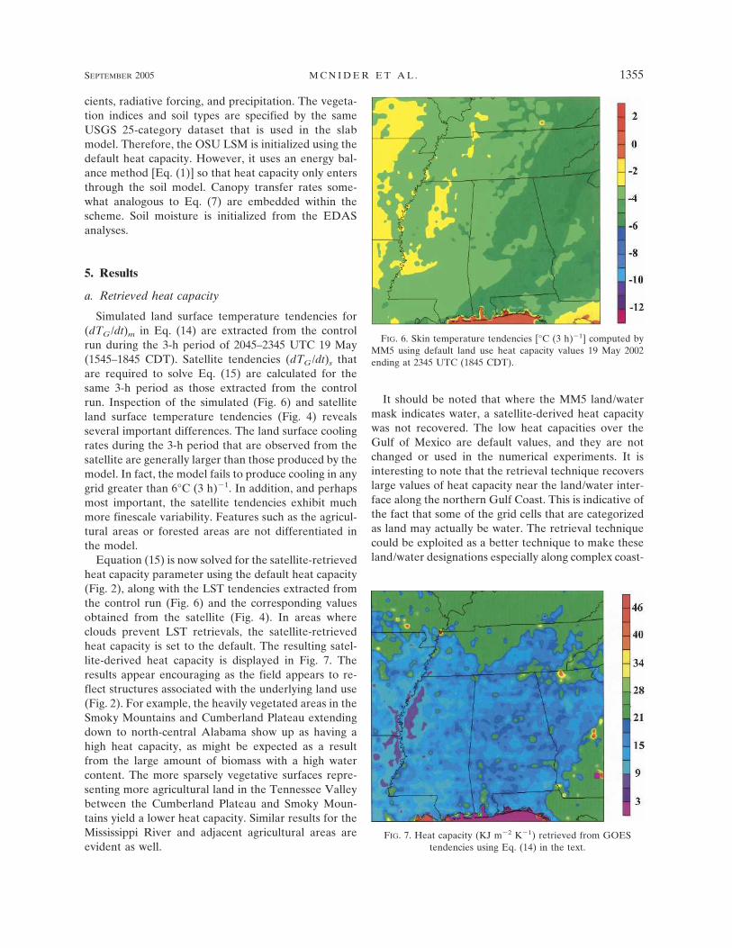
Simulated land surface temperature tendencies for(dTG /dt)m in Eq. (14) are extracted from the controlrun during the 3-h period of 2045–2345 UTC 19 May(1545–1845 CDT). Satellite tendencies (dTG /dt)s thatare required to solve Eq. (15) are calculated for thesame 3-h period as those extracted from the controlrun. Inspection of the simulated (Fig. 6) and satelliteland surface temperature tendencies (Fig. 4) revealsseveral important differences. The land surface coolingrates during the 3-h period that are observed from thesatellite are generally larger than those produced by themodel. In fact, the model fails to produce cooling in anygrid greater than 6°C (3 h) 1. In addition, and perhapsmost important, the satellite tendencies exhibit muchmore finescale variability. Features such as the agricul-tural areas or forested areas are not differentiated inthe model.

Equation (15) is now solved for the satellite-retrievedheat capacity parameter using the default heat capacity(Fig. 2), along with the LST tendencies extracted fromthe control run (Fig. 6) and the corresponding valuesobtained from the satellite (Fig. 4). In areas whereclouds prevent LST retrievals, the satellite-retrievedheat capacity is set to the default. The resulting satel-lite-derived heat capacity is displayed in Fig. 7. Theresults appear encouraging as the field appears to re-flect structures associated with the underlying land use(Fig. 2). For example, the heavily vegetated areas in theSmoky Mountains and Cumberland Plateau extendingdown to north-central Alabama show up as having ahigh heat capacity, as might be expected as a resultfrom the large amount of biomass with a high watercontent. The more sparsely vegetative surfaces repre-senting more agricultural land in the Tennessee Valleybetween the Cumberland Plateau and Smoky Moun-tains yield a lower heat capacity. Similar results for theMississippi River and adjacent agricultural areas areevident as well.

It should be noted that where the MM5 land/watermask indicates water, a satellite-derived heat capacitywas not recovered. The low heat capacities over theGulf of Mexico are default values, and they are notchanged or used in the numerical experiments. It isinteresting to note that the retrieval technique recoverslarge values of heat capacity near the land/water inter-face along the northern Gulf Coast. This is indicative ofthe fact that some of the grid cells that are categorizedas land may actually be water. The retrieval techniquecould be exploited as a better technique to make theseland/water designations especially along complex coast-

FIG. 6. Skin temperature tendencies [°C (3 h) 1] computed byMM5 using default land use heat capacity values 19 May 2002ending at 2345 UTC (1845 CDT).

FIG. 7. Heat capacity (KJ m 2 K 1) retrieved from GOEStendencies using Eq. (14) in the text.


Fig 6 7 live 4/C

lines or marshy areas within the mesoscale model sys-tems.

b. Impact on model performance

The high degree of correlation between the retrievedheat capacities in Fig. 7 and land use type suggest theyappear physical. However, the practical question iswhether the use of these new heat capacities actuallyimproves model performance. The selected case studyis benign, meteorologically, in that there is no precipi-tation and relatively few clouds. As a result, radiativeprocesses play a dominant role in the near-surface tem-perature tendencies. Analysis will focus on the abilityof the models to replicate the observed diurnal cycleover the southeast from 1200 UTC May 19 to 1200UTC 21 May 2002.

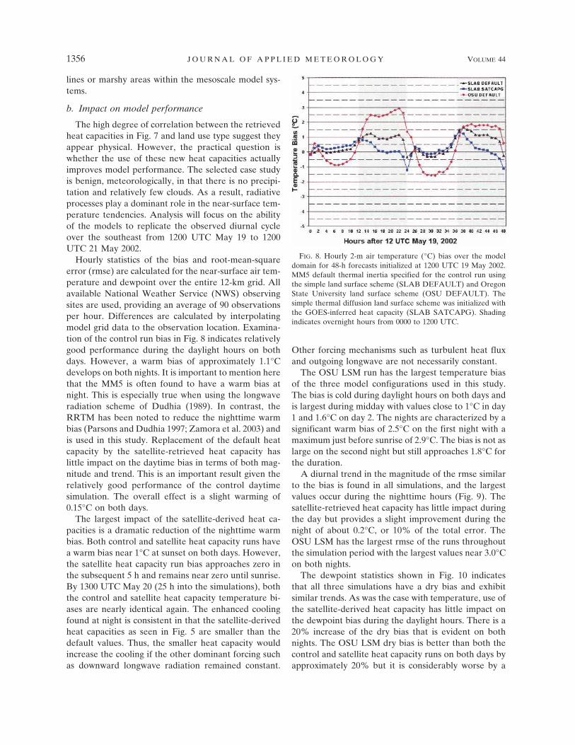
Hourly statistics of the bias and root-mean-squareerror (rmse) are calculated for the near-surface air tem-perature and dewpoint over the entire 12-km grid. Allavailable National Weather Service (NWS) observingsites are used, providing an average of 90 observationsper hour. Differences are calculated by interpolatingmodel grid data to the observation location. Examina-tion of the control run bias in Fig. 8 indicates relativelygood performance during the daylight hours on bothdays. However, a warm bias of approximately 1.1°Cdevelops on both nights. It is important to mention herethat the MM5 is often found to have a warm bias atnight. This is especially true when using the longwaveradiation scheme of Dudhia (1989). In contrast, theRRTM has been noted to reduce the nighttime warmbias (Parsons and Dudhia 1997; Zamora et al. 2003) andis used in this study. Replacement of the default heatcapacity by the satellite-retrieved heat capacity haslittle impact on the daytime bias in terms of both mag-nitude and trend. This is an important result given therelatively good performance of the control daytimesimulation. The overall effect is a slight warming of0.15°C on both days.

The largest impact of the satellite-derived heat ca-pacities is a dramatic reduction of the nighttime warmbias. Both control and satellite heat capacity runs havea warm bias near 1°C at sunset on both days. However,the satellite heat capacity run bias approaches zero inthe subsequent 5 h and remains near zero until sunrise.By 1300 UTC May 20 (25 h into the simulations), boththe control and satellite heat capacity temperature bi-ases are nearly identical again. The enhanced coolingfound at night is consistent in that the satellite-derivedheat capacities as seen in Fig. 5 are smaller than thedefault values. Thus, the smaller heat capacity wouldincrease the cooling if the other dominant forcing suchas downward longwave radiation remained constant.

Other forcing mechanisms such as turbulent heat fluxand outgoing longwave are not necessarily constant.

The OSU LSM run has the largest temperature biasof the three model configurations used in this study.The bias is cold during daylight hours on both days andis largest during midday with values close to 1°C in day1 and 1.6°C on day 2. The nights are characterized by asignificant warm bias of 2.5°C on the first night with amaximum just before sunrise of 2.9°C. The bias is not aslarge on the second night but still approaches 1.8°C forthe duration.

A diurnal trend in the magnitude of the rmse similarto the bias is found in all simulations, and the largestvalues occur during the nighttime hours (Fig. 9). Thesatellite-retrieved heat capacity has little impact duringthe day but provides a slight improvement during thenight of about 0.2°C, or 10% of the total error. TheOSU LSM has the largest rmse of the runs throughoutthe simulation period with the largest values near 3.0°Con both nights.

The dewpoint statistics shown in Fig. 10 indicatesthat all three simulations have a dry bias and exhibitsimilar trends. As was the case with temperature, use ofthe satellite-derived heat capacity has little impact onthe dewpoint bias during the daylight hours. There is a20% increase of the dry bias that is evident on bothnights. The OSU LSM dry bias is better than both thecontrol and satellite heat capacity runs on both days byapproximately 20% but it is considerably worse by a

FIG. 8. Hourly 2-m air temperature (°C) bias over the modeldomain for 48-h forecasts initialized at 1200 UTC 19 May 2002.MM5 default thermal inertia specified for the control run usingthe simple land surface scheme (SLAB DEFAULT) and OregonState University land surface scheme (OSU DEFAULT). Thesimple thermal diffusion land surface scheme was initialized withthe GOES-inferred heat capacity (SLAB SATCAPG). Shadingindicates overnight hours from 0000 to 1200 UTC.


Fig 8 live 4/C

factor of 2 during the nights. The same trends are evi-dent in the dewpoint rmse (not shown).

It is clear from the verification statistics that thesimple slab formulation using the satellite-retrievedheat capacity produced the most realistic surface tem-

perature forecast for this specific event. Results for thedewpoint were not as good as the control run during theevenings, but differed by less than 20%. One could ar-gue that the relatively poor performance of the OSULSM in this case should not be regarded as the norm.The OSU scheme is fundamentally sound in terms ofphysical parameterizations, and numerous studies havereported positive results. The performance of thescheme is obviously sensitive to the specification of sur-face characteristics such as vegetation fraction, rootingdepth, soil types, and soil moisture. No attempt wasmade in this study to develop a modified soil moisturefield using antecedent precipitation analyses. The soilmoisture was initialized in typical fashion using thefields in the EDAS analyses; although, perhaps coarse,it does contain an antecedent precipitation analysis.Given that the focus of this paper is on the nighttimeenergy budget, it is not obviously clear what impactadjusting the OSU soil moisture would have on theresults obtained there from. However, it is noted that aheavy and widespread precipitation event occurred 2days before this case study. Precipitation in excess of0.5 in. (�1.25 cm) fell in a 24-h period ending at 1200UTC 18 May over the majority of the model domain. Ifother offline methods were used to modify EDAS soilmoisture analysis for this event, one would assume anoverall moistening and a reduction of the dry bias in theOSU LSM run. However, it would also be expected toreduce sensible heat fluxes and cause a worsening ofthe cold bias found during the daylight hours underconditions of strong solar forcing.

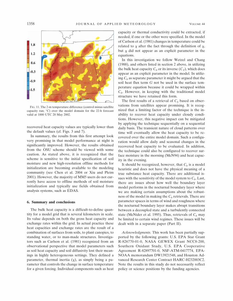
Verification statistics that are presented above areaveraged over the entire model domain, while the sat-ellite heat capacity was only retrieved where skies wereclear at 1545 and 1745 CDT 19 May. Therefore, a per-centage of the observation–model temperature pairsused to calculate the bulk verification statistics are lo-cated within areas where the satellite heat capacitycould not be retrieved and the values were set to thedefault. The spatial distribution of the 2-m temperaturedifference between the control run and the satelliteheat capacity run is used to illustrate the impact ofusing the satellite-retrieved heat capacities. Figure 11shows the difference field in the early morning hoursbefore sunrise at the 22-h forecast that is valid at 1000UTC 20 May when the domain biases were �1.0° and0°C for the control and satellite heat capacity runs, re-spectively. The control 2-m temperature field is foundto be warmer that the satellite heat capacity run and thelargest difference in excess of 1.8°C is found over theagricultural regions along the Mississippi River. Theresponse is consistent with the fact that the satellite-

FIG. 10. Hourly 2-m dewpoint temperature bias (°C) over themodel domain for 48-h forecasts initialized at 1200 UTC 19 May2002. MM5 default thermal inertia specified for the control runusing the simple land surface scheme (SLAB DEFAULT) andOregon State University land surface scheme (OSU DEFAULT).The simple thermal diffusion land surface scheme was initializedwith the GOES-inferred heat capacity (SLAB SATCAPG). Shad-ing indicates overnight hours from 0000 to 1200 UTC.

FIG. 9. Hourly 2-m air temperature (°C) rmse over the modeldomain for 48-h forecasts initialized at 1200 UTC 19 May 2002.MM5 default thermal inertia specified for the control run usingthe simple land surface scheme (SLAB DEFAULT) and OregonState University land surface scheme (OSU DEFAULT). Thesimple thermal diffusion land surface scheme was initialized withthe GOES-inferred heat capacity (SLAB SATCAPG). Shadingindicates overnight hours from 0000 to 1200 UTC.


Fig 9 10 live 4/C

recovered heat capacity values are typically lower thanthe default values (cf. Figs. 3 and 7).

In summary, the results from this first attempt lookvery promising in that model performance at night issignificantly improved. However, the results obtainedfrom the OSU scheme should be viewed with somecaution. As stated above, it is recognized that thescheme is sensitive to the initial specification of soilmoisture and new high-resolution offline methods forinitialization are becoming available to the modelingcommunity (see Chen et al. 2004 or Xiu and Pleim2001). However, the majority of MM5 users do not cur-rently have access to offline methods of soil moistureinitialization and typically use fields obtained fromanalysis systems, such as EDAS.

6. Summary and conclusions

The bulk heat capacity is a difficult-to-define quan-tity for a model grid that is several kilometers in scale.Its value depends on both the gross heat capacity andexchange rates within the grid. In actual practice theseheat capacities and exchange rates are the result of acombination of surfaces from soils, to plant canopies, tostanding water, or to man-made structures. Investiga-tors such as Carlson et al. (1981) recognized from anobservational perspective that model parameters suchas soil heat capacity and soil diffusivity lost their mean-ings in highly heterogeneous settings. They defined aparameter, thermal inertia (), as simply being a pa-rameter that controls the change in surface temperaturefor a given forcing. Individual components such as heat

capacity or thermal conductivity could be extracted, ifneeded, if one or the other were specified. In the modelof Carlson et al. (1981) changes in temperature could berelated to after the fact through the definition of ,but did not appear as an explicit parameter in theequations.

In this investigation we follow Wetzel and Chang(1988), and others listed in section 2 above, in utilizingthe bulk heat capacity Cb or its inverse (CT), which doesappear as an explicit parameter in the model. In utiliz-ing Cb as separate parameter it might be argued that thesoil heat flux term G not be used in the surface tem-perature equation because it could be wrapped withinCb. However, in keeping with the traditional modelstructure we have retained this form.

The first results of a retrieval of Cb based on obser-vations from satellites appear promising. It is recog-nized that a limiting factor of the technique is the in-ability to recover heat capacity under cloudy condi-tions. However, this negative impact can be mitigatedby applying the technique sequentially on a sequentialdaily basis. The transient nature of cloud patterns overtime will eventually allow the heat capacity to be re-covered over the entire model domain. Such a configu-ration would allow daily and seasonal changes in therecovered heat capacity to be evaluated. In addition,the technique could also be configured to recover sur-face moisture in the morning (McN94) and heat capac-ity in the evening.

It should be recognized, however, that Cb is a modelheuristic and does not have the physical meaning of atrue substance heat capacity. There are additional is-sues with the sensitivity of the model system to Cb. Last,there are issues about how well the boundary layermodel performs in the nocturnal boundary layer wherewe are making certain assumptions about the robust-ness of the model in making the Cb retrievals. There areparameter spaces in terms of wind and roughness wherethe nocturnal boundary layer makes abrupt transitionsbetween a decoupled state and a turbulently connectedstate (McNider et al. 1995). Thus, retrievals of Cb maybe limited to certain wind regimes. These issues will bedealt with in a separate paper (Part II).

Acknowledgments. This work has been partially sup-ported by the following grants: U.S. EPA Star GrantR-826770-01-0, NASA GEWEX Grant NCC8-200,Southern Oxidant Study, U.S. EPA CooperativeAgreement R-82897701-0, NSF-ATM-0417774, EPA-NOAA memorandum DW13921548, and Houston Ad-vanced Research Center Contract HARC-H232003C2.Note the results in this study do not necessarily reflectpolicy or science positions by the funding agencies.

FIG. 11. The 2-m temperature difference (control minus satellitecapacity run; °C) over the model domain for the 22-h forecastvalid at 1000 UTC 20 May 2002.


Fig 11 live 4/C

REFERENCES

Argentini, S., P. J. Wetzel, and V. M. Karyampudi, 1992: Testinga detailed biophysical parameterization for land–air ex-change in a high-resolution boundary-layer model. J. Appl.Meteor., 31, 142–156.

Bhumralkar, C. M., 1975: Numerical experiments on the compu-tations of ground temperature in general circulation model. J.Appl. Meteor., 14, 1246–1258.

Black, T. L., 1994: The new NMC mesoscale Eta Model: Descrip-tion and forecast examples. Wea. Forecasting, 9, 265–278.

Blackadar, A. K., 1979: High resolution models of the planetaryboundary layer. Adv. Environ. Sci. Eng., 1, 50–85.

Boone, A., V. Masson, T. Meyers, and J. Noilhan, 2000: The in-fluence of the inclusion of soil freezing on simulations by asoil–vegetation–atmosphere transfer scheme. J. Appl. Me-teor., 39, 1544–1569.

Carlson, T. N., 1986: Regional scale estimates of surface moistureavailability and thermal inertia using remote thermal mea-surements. Remote Sens. Rev., 1, 197–246.

——, J. K. Dodd, S. G. Benjamin, and J. N. Cooper, 1981: Satelliteestimation of the surface energy balance, moisture availabil-ity and thermal inertia. J. Appl. Meteor., 20, 67–87.

Chen, F., and J. Dudhia, 2001: Coupling an advanced land sur-face–hydrology model with the Penn State–NCAR MM5modeling system. Part II: Preliminary model validation. Mon.Wea. Rev., 129, 587–604.

——, K. W. Manning, D. N. Yates, M. A. Lemone, S. B. Trier, R.Cuenea, and D. Niyogi, 2004: Development of a high resolu-tion land data assimilation system (HRLDAS). Preprints,16th Conf. on Numerical Weather Prediction, Seattle, WA,Amer. Meteor. Soc., CD-ROM, 22.3.

Diak, G. R., and C. Gautier, 1983: Improvements to a simplephysical model for estimating insolation from GOES data. J.Climate Appl. Meteor., 22, 505–508.

——, and M. S. Whipple, 1995: Note on estimating surface sen-sible heat fluxes using surface temperatures measured from ageostationary satellite during FIFE 1989. J. Geophys. Res.,100, 25 453–25 461.

Dudhia, J., 1989: Numerical study of convection observed duringthe Winter Monsoon Experiment using a mesoscale two-dimensional model. J. Atmos. Sci., 46, 3077–3107.

——, 1996: A multi-layer soil temperature model for MM5. Pre-prints, Sixth PSU/NCAR Mesoscale Models User’s Workshop,Boulder, CO, NCAR, 49–50.

Garand, L., and Coauthors, 2001: Radiance and Jacobian inter-comparison of radiative transfer models applied to HIRS andAMSU channels. J. Geophys. Res., 106, 24 017–24 031.

Gautier, C., G. R. Diak, and S. Mass, 1980: A simple physicalmodel for estimating incident solar radiation at the surfacefrom GOES satellite data. J. Appl. Meteor., 19, 1005–1012.

Giard, D., and E. Bazile, 2000: Implementation of a new assimi-lation scheme for soil and surface variables in a global NWPmodel. Mon. Wea. Rev., 128, 997–1015.

Grell, G. A., J. Dudhia, and D. R. Stauffer, 1994: The Penn State/NCAR Mesoscale Model (MM5). NCAR Tech. Note NCAR/TN-398�STR, 138 pp.

Guillory, A. R., G. J. Jedlovec, and H. E. Fuelberg, 1993: A tech-nique for deriving column-integrated water content usingVAS split window data. J. Appl. Meteor., 32, 1226–1241.

Haines, S. L., G. J. Jedlovec, and R. J. Suggs, 2004: The GOESproduct generation system. NASA Marshall Space FlightCenter Tech. Memo., NASA/TM-2004-213286, 64 pp.

Hong, S., and H. Pan, 1996: Nonlocal boundary layer verticaldiffusion in a Medium-Range Forecast Model. Mon. Wea.Rev., 124, 2322–2339.

Jacquemin, B., and J. Noilhan, 1990: Sensitivity study and valida-tion of a land surface parameterization using the Hapex-Mobilhy Data Set. Bound.-Layer Meteor., 52, 93–134.

Jedlovec, G. J., 1987: Determination of atmospheric moisturestructure from high-resolution MAMS radiance data. Ph.D.dissertation, University of Wisconsin—Madison, 187 pp.

——, and K. Laws, 2003: GOES cloud detection at the GlobalHydrology and Climate Center. Preprints, 12th Conf. on Sat-ellite Meteorology and Oceanography, Long Beach, CA,Amer. Meteor. Soc., CD-ROM, P1.21.

Jones, A. S., I. C. Guch, and T. H. Vonder Haar, 1998a: Dataassimilation of satellite-derived heating rates as proxy surfacewetness data into a regional atmospheric mesoscale model.Part I: Methodology. Mon. Wea. Rev., 126, 634–645.

——, ——, and ——, 1998b: Data assimilation of satellite-derivedheating rates as proxy surface wetness data into a regionalatmospheric mesoscale model. Part II: A case study. Mon.Wea. Rev., 126, 646–667.

Kain, J. S., and J. M. Fritsch, 1993: Convective parameterizationfor mesoscale models: The Kain–Fritsch scheme. The Repre-sentation of Cumulus Convection in Numerical Models, Me-teor. Monogr., No. 46, Amer. Meteor. Soc., 156–170.

Koster, R. D., and M. J. Suarez, 1992: A comparative analysis oftwo land surface heterogeneity representations. J. Climate, 5,1379–1390.

Lapenta, W. M., R. Suggs, G. J. Jedlovec, and R. T. McNider,1999: Impact of assimilating GOES-derived land surface vari-ables into the PSU/NCAR MM5. Preprints, Workshop onLand-Surface Modeling and Applications to Mesoscale Mod-els, Boulder CO, NCAR, 65–68.

Mahfouf, J.-F., 1991: Analysis of soil moisture from near surfaceparameters: A feasibility study. J. Appl. Meteor., 30, 1534–1547.

——, A. O. Manzi, J. Noilhan, H. Giordani, and M. DéQué, 1995:The land surface ISBA scheme within the Météo-France cli-mate model ARPEGE. Part I: Implementation and prelimi-nary results. J. Climate, 8, 2039–2057.

Mahrer, Y., and R. A. Pielke, 1976: A numerical study of flowover irregular terrain. Contrib. Atmos. Phys., 50, 98–113.

Manzi, A. O., and S. Planton, 1994: Implementation of the ISBAparameterization scheme for land surface processes in aGCM. J. Hydrol., 155, 355–389.

McCumber, M., and R. Pielke, 1981: Simulation of the effects ofsurface fluxes of heat and moisture in a mesoscale model. J.Geophys. Res., 86C, 9929–9938.

McMillin, L. M., and H. E. Fleming, 1976: Atmospheric transmit-tance of an absorbing gas: A computationally fast and accu-rate transmittance model for absorbing gases with constantmixing ratios in inhomogeneous atmospheres. Appl. Opt., 15,358–363.

McNider, R. T., and R. A. Pielke, 1981: Diurnal boundary layerdevelopment over sloping terrain. J. Atmos. Sci., 38, 2198–2212.

——, A. J. Song, D. M. Casey, P. J. Wetzel, W. L. Crosson, andR. M. Rabin, 1994: Toward a dynamic-thermodynamic as-similation of satellite surface temperature in numerical atmo-spheric models. Mon. Wea. Rev., 122, 2784–2803.

——, D. E. England, M. J. Friedman, and X. Shi, 1995: Predict-ability of the stable atmospheric boundary layer. J. Atmos.Sci., 52, 1602–1614.


Menzel, W. P., and J. F. W. Purdom, 1994: Introducing GOES-I:The first of a new generation of geostationary operationalenvironmental satellites. Bull. Amer. Meteor. Soc., 75, 757–781.

Noilhan, J., and S. Planton, 1989: A simple parameterization forland surfaces in meteorological models. Mon. Wea. Rev., 117,536–549.

Norman, J. M., W. P. Kustas, and K. S. Humes, 1995: A two-source approach for estimating soil and vegetative fluxesfrom observations of directional radiometric surface tem-perature. Agric. For. Meteor., 77, 263–293.

Pan, H.-L., and L. Mahrt, 1987: Interaction between soil hydrol-ogy and boundary-layer development. Bound.-Layer Meteor.,38, 185–202.

Parsons, D. B., and J. Dudhia, 1997: Testing of a data assimilationsystem in support of the goals of the Atmospheric RadiationMeasurement Program. Mon. Wea. Rev., 125, 2353–2381.

Peters-Lidard, C. D., E. Blackburn, X. Liang, and E. F. Wood,1998: The effect of soil thermal conductivity parameteriza-tion of surface energy fluxes and temperatures. J. Atmos. Sci.,55, 1209–1224.

Physick, W., 1976: A numerical model of the sea-breeze phenom-ena over a lake or gulf. J. Atmos. Sci., 33, 2107–2135.

Pleim, J. E., and A. Xiu, 1995: Development and testing of asurface flux and planetary boundary layer model for applica-tion in mesoscale models. J. Appl. Meteor., 34, 16–32.

Price, J. C., 1982: On the use of satellite data to infer surfacefluxes at meteorological scales. J. Appl. Meteor., 21, 1111–1122.

Rao, C. R. N., J. Chen, J. T. Sullivan, and N. Zhang, 1999: Postlaunch calibration of meteorological satellite sensors. Adv.Space Res., 23, 1357–1365.

Rogers, E., D. Parrish, Y. Lin, and G. DiMego, 1996: The NCEPEta data assimilation system: Tests with regional 3-D varia-tional analysis and cycling. Preprints, 11th Conf. on Numeri-

cal Weather Prediction, Norfolk, VA, Amer. Meteor. Soc.,105–106.

Smirnova, T. G., J. M. Brown, and S. G. Benjamin, 1997: Perfor-mance of different soil model configurations in simulatingground surface temperature and surface fluxes. Mon. Wea.Rev., 125, 1870–1884.

Suggs, R. J., G. J. Jedlovec, and A. R. Guillory, 1998: Retrieval ofgeophysical parameters from GOES: Evaluation of a splitwindow retrieval technique. J. Appl. Meteor., 37, 1205–1227.

——, S. L. Haines, G. J. Jedlovec, W. Lapenta, and D. Moss, 2003:Land surface temperature retrievals from GOES-8 usingemissivities from MODIS. Preprints, 12th Conf. on SatelliteMeteorology and Oceanography, Long Beach, CA, Amer.Meteor. Soc., CD-ROM, P4.19.

Viterbo, P., A. Beljaars, J. Mahfouf, and J. Teixeira, 1999: Therepresentation of soil moisture freezing and its impact on thestable boundary layer. Quart. J. Roy. Meteor. Soc., 125, 2401–2426.

Wan, Z., and J. Dozier, 1996: A generalized split-window algo-rithm for retrieving land-surface temperature from space.IEEE Trans. Geosci. Remote Sens., 34, 892–905.

Wetzel, P. J., and J.-T. Chang, 1988: Evapotranspiration fromnonuniform surfaces: A first approach for short-term numeri-cal weather prediction. Mon. Wea. Rev., 116, 600–621.

——, D. Atlas, and T. H. Woodward, 1984: Determining soilmoisture from geosynchronous satellite infared data: A fea-sibility study. J. Climate Appl. Meteor., 23, 375–391.

Xiu, A., and J. E. Pleim, 2001: Development of a land surfacemodel. Part I: Application in a mesoscale meteorologymodel. J. Appl. Meteor., 40, 192–209.

Zamora, R. J., and Coauthors, 2003: Comparing MM5 radiativefluxes with observations gathered during the 1995 and 1999Nashville Southern Oxidants Studies. J. Geophys. Res., 108,4050, doi:10.1029/2002JD002122.


Date post:	13-Jun-2018
Category:	Documents
Upload:	vuongtruc
View:	215 times
Download:	0 times

Retrieval of Model Grid-Scale Heat Capacity Using...

Documents