Contents lists available at SciVerse ScienceDirect
Journal of Applied Geophysics
j ourna l homepage: www.e lsev ie r .com/ locate / jappgeo
Retrieval of the physical properties of an anelastic solid half space from seismic data
Gaëlle Lefeuve-Mesgouez a, Arnaud Mesgouez a, Erick Ogam b, Thierry Scotti b, Armand Wirgin b,⁎a Université d'Avignon et des Pays de Vaucluse, UMR EMMAH, Faculté des Sciences, F-84000 Avignon, Franceb LMA, CNRS, UPR 7051, Aix-Marseille Univ, Centrale Marseille, F-13402 Marseille Cedex 20, France
Article history:Received 11 August 2012Accepted 25 September 2012Available online 5 October 2012
Keywords:Nonlinear full wave inversionFive constitutive parametersSeismic dataPrior uncertaintyRetrieval error
In recent years, due to the rapid development of computation hard- and software, time domain full-wave in-version, which makes use of all the information in the seismograms without appealing to linearization, hasbecome a plausible candidate for the retrieval of the physical parameters of the earth's substratum. Retriev-ing a large number of parameters (the usual case in a layered substratum comprising various materials, someof which are porous) at one time is a formidable task, so full-wave inversion often seeks to retrieve only asubset of these unknowns, with the remaining parameters, the priors, considered to be known and constant,or sequentially updated, during the inversion. A known prior means that its value has been obtained by othermeans (e.g., in situ or laboratory measurement) or simply guessed (hopefully, with a reasonable degree ofconfidence). The uncertainty of the value of the priors, like that of data noise, and the inadequacy of thetheoretical/numerical model employed to mimick the seismic data during the inversion, is a source of retriev-al error. We show, on the example of a homogeneous, isotropic, anelastic half-plane substratum configura-tion, characterized by five parameters: density, P and S wavespeeds and P and S quality factors, when aperfectly-adequate theoretical/numerical model is employed during the inversion and the data is free ofnoise, that the retrieval error can be very large for a given parameter, even when the prior uncertainty of an-other single parameter is very small. Furthermore, the employment of other load and response polarizationdata and/or multi-offset data, as well as other choices of the to-be-retrieved parameters, are shown, on spe-cific examples, not to systematically improve(they may even reduce) the accuracy of the retrievals when theprior uncertainty is relatively-large. These findings, relative to the recovery, via an exact retrieval model pro-cessing noiseless data obtained in one of the simplest geophysical configurations, of a single parameter at atime with a single uncertain prior, raises the question of the confidence that can be placed in geophysical pa-rameter retrievals: 1) when more than one parameters are retrieved at a time, and/or 2) when more than oneprior are affected by uncertainties during a given inversion, and/or 3) when the model employed to mimickthe data during the inversion is inadequate, 4) when the data is affected by noise or measurement errors, and5) when the parameter retrieval is carried out in more realistic configurations.
An important branch of activity in geophysics is concerned withobtaining structural (tomographic) images of the subsurface and esti-mating the physical properties of the different layers. Although struc-tural details can be obtained by the migration of (either man-made ornatural) seismic data (a process that employs only a small amount ofthe information in the seismogram), retrieving the physical propertiesof the geological formations (as is important, for instance, in hydrocar-bon exploration and prediction of seismological site effects) requires aseismic inversion method (Forbriger, 2003; Sacks and Symes, 1987;Tarantola, 1986). Travel-time inversion (TTI; which also uses only asmall amount of the information in the seismogram, i.e., the pickedtravel times) (Bodet, 2005; Foti et al., 2009; Luo and Schuster, 1991;
.
rights reserved.
Pereyra et al., 1980; Xia et al., 1999) or full waveform inversion (FWI;which employs most or all of the information in the seismogramand does not require fastidious and sometimes ambiguous travel-timepicking) techniques have been employed either separately (De Barroset al., 2010; Delprat-Jannaud and Lailly, 2005; Dupuy, 2011; Jeong etal., 2012; Mora, 1987; Pratt, 1999; Sebaa et al., 2006; Song et al., 1995;Sun and McMechan, 1992; Virieux and Operto, 2009) or together withTTI (Buchanan et al., 2011; Chotiros, 2002; Dessa and Pascal, 2003;Korenaga et al., 1997) to retrieve wave-mechanical parameters of thesubstratum, such as Poisson's ratio, density, quality factors and bodywave velocities, by minimizing the differences between real (eithermeasured or synthetic) and trial seismic data generated by a more-or-less rigorous wave propagation model together with a subsurfacemodel of supposedly-appropriate structure and composition.
An annoying problem in the characterization of the substratum isthe large number of unknown parameters; this is termed the ‘curseof dimensionality’ in (Curtis and Lomax, 2001). A typical inversion
71G. Lefeuve-Mesgouez et al. / Journal of Applied Geophysics 88 (2013) 70–82
algorithm assumes that most of the parameters are known a priori(these parameters are termed priors (Scales and Tenorioz, 2001)); inSebaa et al. (2006) six out of eleven of the porous medium parametersare treated as fixed priors, so that the inversions are carried out onlyfor the remainingfive parameters, in (Aoi et al., 1995) the basin velocitiesand details of the solicitation are treated as fixed priors during the deter-mination of the basin shape, and in (Burstedde and Ghattas, 2009) and(Kolb et al., 1986) the density is treated as a known, fixed prior duringthe retrieval of the velocity (or rigidity) distribution in a 1D acoustic(or elastic) medium. Another option is to assume that certain priors arerelated in some manner (such as in a Poisson solid) and the remainingparameters are sought-for in a rather large parameter search space.
Similar remarks apply to the to-be-retrieved parameters. The initialestimation of the latter is often far-removed from reality, but can be re-fined by the reduction of the size of the parameter search space, where-in the trial data is again compared to the real data to obtain a secondestimation of the unknown parameters. This iterative process, withthe set of priors conserving their initial values, is repeated as manytimes as necessary to obtain some pre-assigned estimation accuracy.
Another approach to multiparameter retrieval, which seeks toalleviate somewhat the ‘curse of dimensionality’, proceeds in aso-called sequential fashion (De Barros et al., 2010; Forbriger, 2003;Kormendi and Dietrich, 1991). Suppose the number of parameters istwo. In the first step, p1 is treated as a known prior (the notion of‘known’ can have many meanings ranging from ‘measured’ (e.g., someof the Biot parameters in Buchanan et al., 2011) to ‘guessed’ (e.g., thequality factors in (Forbriger, 2003)) and the inversion is carried outonly for p2. In the second step, the retrieved value of p2 is treated as aprior and the inversion is carried out to retrieve p1. In the third step,the newly-retrieved value of p1 is treated as a prior and the inversionis carried out for p2. This procedure could go on indefinitely, but usuallystops at an early level. First attempts at a critical analysis of this tech-nique were carried out in (Le Marrec et al., 2006), but gave rise to noconvincing conclusion. It seems reasonable to expect that this iterativeprocedure will diverge if at the initial stage, the inversion alreadyleads to highly-erroneous results for p2 due to relatively-large uncer-tainty in the prior p1.
Inversion algorithms such as the procedures described above, arenot easy to implement, in that they usually demand manual surveil-lance and intervention. Moreover, at each step, an interpretationproblem can arise, as attested by the fact that the algorithm cangive rise to three types of results (Wirgin, 2004): 1) either the re-trievals are obtained without any apparent difficulty, i.e., at most iter-ation steps, the discrepancy function resembles a single paraboloid(in the parameter search space) with a well-defined minimum(Sebaa et al., 2006), 2) the discrepancy function does not exhibit a pa-raboloid type of behavior in the successive parameter search spaces sothat no estimation can be made of the sought-for parameters, or3) the discrepancy functions exhibit several local minima (Buchananet al., 2011; Ogam et al., 2001, 2002) so that a decision has to be madeas to which minimum is the most appropriate.
It has been shown (Buchanan et al., 2002; Groby et al., 2011;Ogam et al., 2001; Wirgin, 2004) on some rather simple examplesof inverse problems, that: a) the most favorable situation (case 1)occurs when the retrieval model gives rise to data that is as closeas possible to the real data throughout the parameter searchspace, and b) the least favorable situations (cases 2) and 3)) occurwhen the retrieval model gives rise to data that is significantly dif-ferent from the real data in a part of, or throughout, the parametersearch space. Interestingly enough, efforts (Buchanan et al., 2000,2002; Scotti and Wirgin, 1995; Wirgin and Scotti, 1996) have beenmade to deliberately employ a retrieval model that is different, byits theoretical and numerical ingredients, from the model used toobtain synthetic data, notably to avoid what in (Colton and Kress,1992) is termed a ‘trivial solution’ to the inverse problem. Avoid-ance of ‘trivial solutions’ can also be obtained by artificially
introducing noise into the synthetic data (Aoi et al., 1995;Buchanan et al., 2002). However, such efforts are generally deemednot necessary, or the issue of ‘trivial solutions’ is simply sidetracked(Aoi et al., 1995; De Barros et al., 2010; Sebaa et al., 2006) by the useof the same theoretical/numerical scheme for the simulation andthe retrieval of the unknown parameters.
The present investigation addresses the issue of the effect of prioruncertainty on the accuracy of parameter retrieval. This type of studywas initiated in (Aoi et al., 1995; Buchanan et al., 2002, 2011;Chotiros, 2002; De Barros et al., 2010; Dupuy, 2011; Jeong et al.,2012; Scotti and Wirgin, 2004) and usually relies on synthetic datathat is created with the same theoretical/numerical model as theone employed for the retrievals. Although this seems to imply that a‘trivial solution’ is generated, it can be argued that prior uncertaintyhas an effect somewhat equivalent to introducing a difference be-tween the two models.
The chosen geophysical configuration herein is a homogeneous,isotropic, anelastic half-space (i.e., the underground or substratum)solicited by a transient load on its flat boundary (i.e., the ground)which generates seismic waves acquired by receivers located on thisboundary. Five reasons explain this choice.
1 Although it is unrealistic in the context of natural resource explora-tion, it has been employed to examine various aspects of a varietyof other applied geophysical problems (de Barros et al., 2010;Goldman et al., 1996; Hurley and Spicer, 2004; Kozhevnikov andAntonov, 2008; Muijs et al., 2002; Wu et al., 2001), notably to fur-nish a macromodel (reference) medium for the backgroundGreen's function employed in tomographical imaging (via Born orRytov schemes) of a layer-like or bounded heterogeneity in an oth-erwise macroscopically-homogeneous underground (Cox, 1991;Gelis, 2005; Gelis et al., 2007; Operto et al., 2004; Ribodetti andVirieux, 1998; Van der Made, 1988). Note that in most of thelatter-cited references, the background medium is assumed to beknown beforehand, whereas, in field experiments it is usually asunknown as the layer-like or bounded heterogenities containedtherein, a fact that explains why the physical parameters of thebackground must be retrieved by inversion before proceeding tothe imaging of the heterogeneities.
2 Thehomogeneous, isotropic half space configuration is often used (andcalled the Okada model Okada, 1985) to estimate earthquake sourceparameters from geodetic data (Amoruso et al., 2004; Feigl, 2002).
3 It can also be of interest to seismologists concerned with predictingearthquake site effects, since the concept of amplification of groundmotion is often related (Bard and Tucker, 1985; Boore, 1972;Bouchon, 1973; Fäh et al., 1994; Geli et al., 1988; Kawase and Aki,1989) to a ratio of motion at a point on a ground that is not flat(i.e., on a hill or in a basin) and/or overlies relatively soft layers(i.e., an alluvial basin or a weathered hill) to the motion at apoint on flat ground overlying hard rock, and in order for these ra-tios to be meaningful, the mechanical parameters of the rock (over-lain by flat ground) have to be identified beforehand.
4 The use of the geophysically-unrealistic homogeneous, isotropichalf plane model provides one of the simplest illustrations (asshown hereafter) of the deleterious effect of prior uncertainty onsubsurface parameter retrieval error, and these effects are surelyof the same order or even of greater order in more complicated,more realistic (e.g., vertically or laterally-inhomogeneous) subsur-face configurations as arise in field experiments (Delprat-Jannaudand Lailly, 2005; Van Vossen et al., 2004).
5 Seminal contributions to nonlinear FWI such as (Kolb et al., 1986;Tarantola, 1984) relied on the more drastic elements of unrealityconstituted by the acoustic approximation, and/or infinite qualityfactors (Tarantola, 1986).
Although inversion necessarily appeals to a theoretical/numericalapparatus for solving the forward problem, we shall only briefly recall
72 G. Lefeuve-Mesgouez et al. / Journal of Applied Geophysics 88 (2013) 70–82
the essential aspects of the latter, while directing most of our atten-tion towards bringing to light several important features of the corre-sponding inverse seismic wave problem.
This will be done by addressing the issue of the retrieval of the fivewave-mechanical parameters (density, real parts of the P and S bodywave velocities and quality (Q) factors) of the solid substratum, as-sumed to exhibit constant Q over the range of considered frequencies,when the solicitation takes the form of a Ricker pulse transient stressof uniform amplitude over a strip giving rise to P and SV waves withinthe subsurface and on the ground. The retrieval is accomplished by pro-cessing simulated temporal response (the signal data) acquired on theground. The distance between the location of the receiver(s) and the lo-cation of the load, as well as the geometrical and physical properties ofthe latter, are assumed to be perfectly well-known.
We shall determine to what extent a nonlinear time domain FWImethod enables the retrieval, one at a time, of these five positivereal wave-mechanical parameters of the substratum when anotherparameter is not well-known a priori. Finally, we address the ques-tions of whether the employment of: a) various types of signal datacorresponding to different types of load and b) different componentsof the field, as well as c) multiple offset data, and d) different choicesof the to-be-retrieved parameters, are capable (or not) of reducingthe retrieval error for given prior uncertainties.
2. Statement of the inverse problem
2.1. The two models
In order to carry out an inversion of a data set one must dispose ofa model of the physical process which can accurately mimick the data.We term this model, the retrieval model, or M. M is characterized byits mathematical ingredients M and numerical ingredients N.
When, as in the present study, the (true) data is not the result of ameasurement, it must be generated (simulated), again with the helpof a model of the underlying physical process which is thought to beable to mimick the true data. We term this model, the data simulationmodel, orm.m is characterized by its mathematical ingredientsm andnumerical ingredients n.
Eachmodel involves a certain number of physical/geometric param-eters: those ofm andM are p and P respectively. The object of a typicalinversion is to retrieve a subset r of P by varying the corresponding sub-set R (whose cardinal is equal to that of r) of P so as to minimize amea-sure of the discrepancy between the synthetic data set d issuing frommand n, and a trial data set D generated by M, it being understood thatd=d(q,r) is fixed and D=D(Q,R) is variable during the inversion,with q=p−r and Q=P−R the remaining parameters (called ‘priors’,both fixed during an inversion) of the two models.
2.2. The inverse crime
In our study, as in many other inverse problem investigations (Aoiet al., 1995; Buchanan et al., 2011; De Barros et al., 2010; Groby et al.,2011; Ogam et al., 2001; Ogam et al., 2002; Scotti and Wirgin, 2004;Sebaa et al., 2006), M and N of the retrieval model are chosen to bethe same as m and n respectively of the data simulation model. Inthis case, the response computed via M turns out to be identical tothe response computed via m.
A corollary of this result, of importance in the inverse problem con-text (Colton and Kress, 1992;Wirgin, 2004), can be stated as follows: ifa)M andN of the retrieval model are chosen to be the same asm and nrespectively of the data simulation model, b) the values of all the priorsQ are known (or chosen) to be equal to their counterparts q, then theinversion should give rise to at least one solution, R=r. Carrying outan inversion by assuming a)+b) has been termed the ‘inverse crime’in (Colton and Kress, 1992) wherein it is written that it leads to the sin-gle ‘trivial solution’ R=r. In (Buchanan et al., 2002, 2011; Ogam et al.,
2001; Ogam et al., 2002; Wirgin, 2004) it was shown that committingthe inverse crime can also lead either to no solution or tomore-than-one solutions.
The eventuality of committing the inverse crime is highly improb-able in real-life in that one usually has only a vague idea a priori of thevalue of at least one of the parameters of the set q of priors. This is thereason why, in the present study, we take explicitly into account thisuncertainty (the avoidance of the inverse crime is not our principalconcern herein).
2.3. The salient features of our inversion procedure
The data processing aspect of inversion is iterative in the sensethat the variation of R is accomplished in successive steps so as toprogressively reduce the discrepancy (or cost) K between the trialsignal D and data signal d. There exist many techniques for doingthis: the one adopted in the present investigation is to: 1) first con-strain R within the parameter search space S and search for the R,amongst the setG of all the R on a grid spanningS, which correspondsto the minimum value of K on this grid, 2) then either shift, and/or re-duce the size of S, and/or increase the number of grid points within S,and 3) re-do the first step by searching the minimum of K in the newS, 4) again shift, and/or reduce the size, and/or increase the number ofgrid points of S as in the second step, and generally carry out thesestep-by-step actions as many times as is necessary to get an estima-tion, with prescribed precision, of the location of the minimum.
It can happen that relative (or local) minima of the discrepancyfunctional K occur at more than one point withinS. The way we elim-inate this non-uniqueness is to (somewhat arbitrarily) choose, ateach step of the iterative procedure, the point R at which K attains aglobal minimum (in the current S) to be “the (retrieved) solution”(denoted by er) of the inverse problem.
The initial choice of S is related to the knowledge one has before-hand of the values of the target parameters of the set r: the more heknows about these parameters, the smaller one chooses S. On theother hand, if one knows little about these parameters, S is larger(say, S′), and the number of local minima of K within S′ can also belarger than those in S, with the possibility that a former global mini-mum of S becomes a local minimum of S′. This means that the choiceof S also affects the outcome of the inversion.
An issue of some importance concerns the duration of the signals dand D employed during the inversion. When the data signal is syn-thetic in nature, its duration can usually be chosen at will, contraryto a real data signal, whose duration is usually imposed by physicalor economic constraints. Trial data signals generated during the in-version, like the synthetic data signal, can have any duration, but, ofcourse, it makes no sense to choose the latter to be longer than thatof the synthetic (or real) data signal. In fact, it is convenient to choosethe two durations to be equal to one and the same value, T= te− tb,with tb,te being the beginning and end instants of the data signal.There remains the choice of suppressing either early (usually bodywave) or late (usually surface wave) arrivals; in fact, we choose tosuppress neither since full wave inversion, by definition, takes intoaccount the entire signal (the latter is cut off at times beyond whichits amplitude is very small, e.g., 60 dB below the maximum). Thismeans that we attempt to retrieve the unknown parameters byinverting both body waves and surface waves (in our configuration,one direct P body wave, one direct S body wave, and one Rayleighsurface wave attain a receiver located on the ground).
Since the positions of the receivers and their number condition thequality and amount of data that is employed in the inversion, thesefactors will also have an effect on the outcome of the parameterretrievals.
The last point concerns the sampling density of the data. Thisquantity is chosen to account for all the significant detail of the signal.
73G. Lefeuve-Mesgouez et al. / Journal of Applied Geophysics 88 (2013) 70–82
In fact, the latter is characterized by three parameters, T:=(tb, te, tm),with tm being the number of equidistant sampling points in [tb,te].
2.4. Cost functional for single or multi-offset data
L (≥1) sensors are located at the points X={xl;l=1,2,…,L}(assumed to be on the ground) and acquire the data during Tl:=(tbl,tel,tml), with T:={Tl;l=1,2,…,L}. Let s(p;xl,t);t [tdl,tel] be thedata signal acquired at the l-th sensor and S(P;xl,t);t [tdl,tel] the cor-responding trial signal. Our choice of cost functional is
K p;P;T;Xð Þ ¼ K p;P;Tl;Xð Þk p; T;Xð Þ ¼
∑Ll¼1
1Tl∫teltbl
s p; xl; tð Þ−S P; xl; tð Þ½ �2dt
∑Ll¼1
1Tl∫teltbl
s p; xl; tð Þ½ �2dt: ð1Þ
Note that K depends explicitly on T and X. Normally speaking, italso depends on the way the integrals are computed, but we assumethat this can be done with any degree of precision (we actuallyemployed a Simpson quadrature scheme with tm points).
2.5. Minimization of the cost functional
The inverse problem is solved by minimization of the cost func-tional. The global minimum of the cost functional (in the search re-gion) is found for R ¼ r̃, i.e.,
r̃ Q ;G; T;Xð Þ ¼ argminR⊂G
K p;P; T;Xð Þ; ð2Þ
wherein G designates the set of all the values assumed by R on thegrid spanning S during a given minimum search process.
Note that r̃ depends explicitly on: a) the choices of the priors Q,b) the search space S via G, c) the sampled signal parameters T,d) the number and positions of the receivers, and implicitly on p.
The arg symbol in front of the min symbol means that the actualvalue of the minimum of K is irrelevant other than the requirementthat it be a global minimum; rather it is the R which produces thisglobal minimum that is the item of interest.
It follows that
K p;p;T;Xð Þ ¼ 0; ð3Þ
since themathematical/numerical models underlying s andS are hereinassumed to be identical and thus give rise to the same signals for P=p.This implies that when Q=q (i.e., the priors are equal to their truevalues), the result of the inversion should lead to at least one solution(Wirgin, 2004) R ¼ r̃ which happens to be the true solution r.
2.6. Definition of the precision of the parameter retrieval and prioruncertainty
Our aim herein is to evaluate the relative error of the retrieved pa-rameter erkεjk :¼ erk δj
� �−rk
rk;ð4Þ
as a function of the relative prior uncertainty, which, for a prior Qj∈ Q,is
δj :¼Qj−qjqj
: ð5Þ
In our problem, the true values of the five physical parameters ofinterest (density, real part of the shear (S) body wave velocity, real
part of the compressional (P) body wave velocity, S wave quality fac-tor, P wave quality factor) are:
but we also examine the opportunity of replacing qP by gP:=1/qP andqS by gS:=1/qS.
We assume that one of these parameters is retrieved at a time(i.e., the parameter search space S is the segment of a line) andthat the four other parameters are priors, one of which is affectedby uncertainty and the other three equal to their true values.
Thus, for instance if we want to retrieve ρ in the caseRcS is an un-certain prior, then, r={p1=ρ}, R={P1=R}, Q={Q2=p2= RcP ,Q3=Rcs, Q4=qP, Q5=qS}.
For each assumed type of solicitation and wavefield component,the matrix ε is composed of 25 elements εjk, 20 of which (i.e., theoff-diagonal elements) are meaningful. The latter are obtained by acomplete inversion process for the k-th parameter (amongst thefive possible unknown parameters) with all the priors being exactlyequal to their true values except the j-th prior (amongst the five pos-sible priors) which is affected by the relative uncertainty δj. Thus, forinstance, ε35 is the relative error of er5 ¼ eqS, resulting from the inver-sion carried out for the single parameter qS during which all the priorsare equal to their true values exceptRCs whose relative uncertainty isδ3 ¼ δRCs .
3. Ingredients of the data simulation and retrieval models
We now give a brief description of the theoretical and numericalingredients of M and m. Most of the material in this section can befound scattered throughout the geophysical literature and, in particu-lar, in (Achenbach, 1973; Bouchon, 1981; Groby, 2005; Kennett,2001; Mesgouez, 2005; Rayleigh, 1885).
3.1. The setting
The medium M occupying the lower half space Ω, is a linear, iso-tropic, homogeneous, anelastic solid and the medium occupying theupper half space R3\Ω is the vacuum. The constitutive mechanical pa-rameters ofM are: ρ (mass density) and λ, μ (Lamé parameters). Dueto the assumed homogeneous, isotropic, anelastic nature of M, ρ is areal scalar constant, and λ, μ are complex scalar constants (whoseimaginary parts are negative) with respect to position x:=(x1, x2,x3) in Ω. The origin O of the Cartesian coordinate system is on theground G constituting the flat horizontal interface between the twohalf spaces. U={Um(x,t);m=1,2,3} designates the displacement(a vector) in M, with spatial derivatives Uk,l:=∂Uk/∂xl. Note, thatthe dependence of U on p (or P) is implicit.
The medium is solicited by stresses applied on the portion Ga of G.Other than on Ga, the boundary G is stress-free. In addition, we as-sume that: Ga is an infinitely long (along x2) strip located betweenx1=−a1 and x1=a1 and the applied stresses are uniform, so thatthe stresses and the displacement U depend only on x1 and x3, i.e., theproblem is two-dimensional. Thus, from now on, the focus is on whathappens in the sagittal (x1–x3) plane and on the linear traces Γ of Gand Γa of Ga (see Fig. 1). Moreover, the vector x is now understood toevolve in the sagittal plane, i.e., x=(x1, 0, x3) and all derivatives of dis-placement with respect to x2 are nil.
74 G. Lefeuve-Mesgouez et al. / Journal of Applied Geophysics 88 (2013) 70–82
3.2. The boundary value problem
The time-domain elastodynamic field U is related to itsfrequency-domain counterpart u by
U x; tð Þ ¼ ∫∞−∞
u x;ωð Þ exp −iωtð Þdω; ð8Þ
(ω the angular frequency), with u satisfying the elastodynamic waveequation (Eringen and Suhubi, 1975):
which are recognized to be the velocities of the transverse (shear,Secondary) (i.e., cS) and longitudinal (compressional, Primary) (i.e.,cP) bulk waves in M. The anelastic nature of M entails that cP,S arecomplex, i.e., cP,S=cP,S
r + icP,Si , with crP;S ¼ RcP ;S ≥0.
The quality factors of the P and S waves are defined in (Kennett,2001) as
QS :¼ −RμIμ
;QP :¼ −R λþ 2μð ÞI λþ 2μð Þ ; ð15Þ
Fig. 1. Description of the problem in the sagittal plane.
and assumed to be constants (Aki and Richards, 1980; Liu et al., 1976)in the range of seismic frequencies considered hereafter (they arealso scalar constants with respect to position in the substratum, dueto the assumed homogeneous, isotropic nature of M).
3.4. Solution for the displacement response on the ground
By employing the Helmholtz decomposition, the gauge condition,the radiation condition, and the boundary conditions, we obtain thefollowing solutions for the in-plane displacement field on theground:
u1 x1;0;ωð Þ :¼ u11 x1;0;ωð Þ þ u13 x1;0;ωð Þ ¼
4iα1H ωð Þμ
∫∞0
P1χSr2S cos ξωX1ð Þ þ P3iξ ξ2−χ2
S þ 2χPχS
� �sin ξωX1ð Þ
h i sinc ξωAð ÞD ξð Þ dξ;
ð16Þ
u3 x1;0;ωð Þ :¼ u31 x1; 0;ωð Þ þ u33 x1;0;ωð Þ ¼
4iα1H ωð Þμ
∫∞0
−P1iξ ξ2−χ2S þ 2χPχS
� �sin ξωX1ð Þ þ P3χPr
2S cos ξωX1ð Þ
h i sinc ξωAð ÞD ξð Þ dξ;
ð17Þ
wherein: sinc xð Þ :¼ sinxx ; A :¼ a1
cq; Xj :¼
xjcq; cq is a reference velocity
with no particular characteristics other than Rcq > 0;Icq ¼ 0;
3.4.1. Numerical issues concerning the computation of the transfer functionEqs. (16)–(17) tell us that
umn x1;0;ωð Þ ¼ H ωð ÞTmn x1;0;ωð Þ; ð24Þ
wherein T mn x1;0;ωð Þ is the transfer function (in the form of an inte-gral I involving ξ spanning [0,∞]) for component m of the displace-ment field in response to the applied stress σn3.
Various strategies have been devised (Bouchon, 1981; Groby,2005; Groby and Wirgin, 2005; Lefeuve-Mesgouez et al., 2012; Xuand Mal, 1987) to compute such integrals, many of which take specif-ic account of the possible (generally-complex) solution ξR of D(ξ)=0.Our choice, somewhat similar to the one in (Lefeuve-Mesgouez et al.,2012), was to subdivide the integral I into three parts: I1 in which ξ
75G. Lefeuve-Mesgouez et al. / Journal of Applied Geophysics 88 (2013) 70–82
spans [0,ξ1], I2 in which ξ spans the interval [ξ1,ξ2] including RξR(determined by finding the value of ξ for which 1/‖D(ξ)‖ attains itsmaximum), and I3 in which ξ spans [ξ3,ξ∞] with ξ∞ chosen largeenough for the integrand of I3 to be negligibly small at ξ=ξ∞. Thethree integrals were carried out by the Simpson quadrature scheme.The integrand in I1 is well-behaved so that I1 requires a relatively-small amount of quadrature points. The integrand in I2 is in theform of a quasi-Gaussian function due to the resonance at ξ=ξR sothat I2 requires a relatively-large amount of quadrature points(all the larger, the larger are QP and QS). The integrand of I3 is ahighly-oscillating function so that I3 requires an even larger amountof quadrature points (all the more so, the higher is the frequency),notably to satisfy the Shannon criterion.
3.5. The displacement signal (space-time representation of the displacementfield) on the ground
Eqs. (12), (16)–(20) show that
umn x1;0;−ωð Þ ¼ umn x1;0;ωð Þ; m;n ¼ 1;3 ; ð25Þ
(the overbar symbol designating the complex conjugate operator) sothat the space-time displacement field on the ground (see Eq. (8))takes the form
This expression (in which um1 applies to P3 ¼ 0 and um3 to P1 ¼ 0in Eqs. (16)–(17)) involves (via umn (x1,0,ω)) the pulse spectrumH ωð Þ. In the results presented hereafter, we chose the load signal tobe that of a Ricker pulse h(t)=[1−2α2(t−β)2]exp[−α2(t−β)2]whose spectrum is
H ωð Þ ¼ ω2
4α3 ffiffiffiπ
p exp iβω− ω2
4α2
!: ð27Þ
3.5.1. Numerical issues concerning the computation of the response signalThe integral in Eq. (26) requires truncation of the infinite interval
to [0,2πf∞], wherein f∞ is chosen large enough for the integrand to benegligible at this value of f ¼ ω=2π. The integral was then computedby the Simpson quadrature scheme, with the number of points cho-sen in such a way as to satisfy the Shannon sampling criterion.
Our numerical results for the space-time domain response com-pared very favorably with those of (Groby, 2005; Hurley and Spicer,2004; Levander, 1988; Robertsson, 1996; Virieux, 1986).
4. Numerical results
In all that follows, the five true parameters (employed to generatethe data and constituting the targets of the inversions) are:
Other parameters, considered to be perfectly-well known, andfixed during all the inversions, are: the width of the load segmenta1=0.1 m, and the Ricker pulse parameters α=250 s−1, β=0.02 s. The data employed in the retrievals consisted of several hun-dred samples of either the horizontal or vertical components of dis-placement in the temporal window of several tenths of a second inresponse to either a vertical or horizontal load.
For the to-be-retrieved parameter r, the grid in the search region isdefined by (rb, re, rm), where rb, re are the minimum and maximum
values of r, and rm is the number of grid points between (and including)these two values.
We employed both U11 data and U33 data, although separately, tocompute the elements of the ε matrices. This was done for bothmono- and multi-offset data.
4.1. Examples of response signals
In Fig. 2, we give an example of the response signals obtained inthe manner outlined in the previous section.
4.2. Illustration of the inversion process for mono-offset data
Inmost of our inversions, we assume (as is not often the case in pub-lished parameter retrieval studies) that little is known about the actualvalue of the to-be-retrieved parameter, which means that we choosethe initial search space S (which is a segment, due to the fact that weretrieve only one parameter at a time) to be very large.
The following three figures, i.e., Figs. 3–5, relative to the retrievalof ρ for uncertainty affecting the prior RcS, illustrate how the inver-sion process was carried out, i.e.:
1 generate the data once and for all (red curve in the top panel of thefigures);
2 for each trial value on the grid spanning S, generate the responsefunctions (blue curves in the top panel of the figures);
3 compute the cost functional K corresponding to the set of bluecurves and plot these K as a function of the trial values (bluecurve in the lower panel);
4 find the position (argmin) of the globalminimumof the cost functionwhen K exhibits a parabolic shape or else shift and reduce/expand S;
5 repeat operations 2–4 until K exhibits a parabolic shape in S; if nosuch shape is obtained after a reasonable amount of changes of S,abandon the procedure and accept the fact that the inversion can-not succeed, or else;
6 to more precisely locate r̃, reduce the size of S, while keeping con-stant or increasing the number of trial values therein, and repeatoperations 2–5 (Figs. 2 to 5);
7 the adopted value of the sought-for parameter, i.e., r̃ correspondsto the position of the minimum of the cost function in the last ofthe three figures.
4.2.1. Comments on the set of figures relative to a successful parameterretrieval
The preceding set of figures shows that:
1 the route to a successful parameter retrieval is all but rectilinear inthat often one must make several adjustments (i.e., shifts) of theparameter search space during the successive phases of the inver-sion process, even when the initial S is quite large; these actionsare difficult to automate on a computer, which in fact explainswhy nonlinear full-wave parameter retrieval in the presence ofprior uncertainty cannot, in our opinion, be carried out withouthuman supervision;
2 in the top panel of Fig. 5, one observes that the blue trial curve, corre-sponding to thefinal retrieved value of ρ, is quite ‘close’ to the red datacurve; this has been taken to imply in other investigations (Korenagaet al., 1997; Mora, 1987; Sebaa et al., 2006) that the retrieved param-eter is close to its true value, although it can be seen here that this isnot necessarily the case since the final eρ ¼ 3010 kg=m3 is rather farfrom the true ρ=2750 kg/m3.
4.3. Graphs relating εjk to δj for mono-offset data
The graphs in Figs. 6–9 relate εjk to δj for various j and k. The rangeof relative uncertainties |δj| does not exceed 0.1 in these figures.
0 0.05 0.1 0.15−4
−2
0
2
4x 10⁻¹²
t(s)
U11
0 0.05 0.1 0.15−6
−4
−2
0
2x 10⁻¹²
t(s)
U31
0 0.05 0.1 0.15−2
0
2
4
6x 10
−12
t(s)
U13
0 0.05 0.1 0.15−5
0
5x 10
−12
t(s)
U33
Fig. 2. The dotted black curve in each panel is the Ricker load signal (actual amplitude equal to one, but, for the purpose of display in the figure, normalized with respect to themaximum of response). The blue curves are the predicted in-plane motion response signals on the ground at x1=300 m: U11, U31, U13, and U33 (amplitudes in arbitrary units).The green and cyan lines indicate the theoretical times of arrival of the P and S body waves respectively, whereas the magenta line indicates the theoretical time of arrival ofthe Rayleigh surface wave. (For interpretation of the references to color in this figure legend, the reader is referred to the web version of this article.)
76 G. Lefeuve-Mesgouez et al. / Journal of Applied Geophysics 88 (2013) 70–82
4.3.1. Comments on the graphs of εjk versus δjAn absolute uncertainty of 0.05 for a given prior is reasonably small,
but our graphs show that even such a small uncertainty can lead tocatastrophically-large relative retrieval errors for certain parameters.For other parameters, this situation is obtained for even smaller abso-lute uncertainty of the prior. The retrieval errors are observed to bevery different for positive uncertainties than for negative uncertainties.
These findings will be illustrated in numerical fashion in the tableswhich follow.
0 0.02 0.04 0.06 0.−1.5
−1
−0.5
0
0.5
1
1.5x 10⁻¹¹
t(
U
1000 1200 1400 1600 1800 200
1
2
3
4
cost
Fig. 3. Inversion of U33, acquired at one sensor located at x1=300 m, to retrieve ρwhen the uspace S such that r=(1000 kg/m3,3000 kg/m3,11)) in the inversion process. Top panel: datfunctional K corresponding to the responses for the various trial values of ρ. Note that K exhwill occur for larger ρ. (For interpretation of the references to color in this figure legend, th
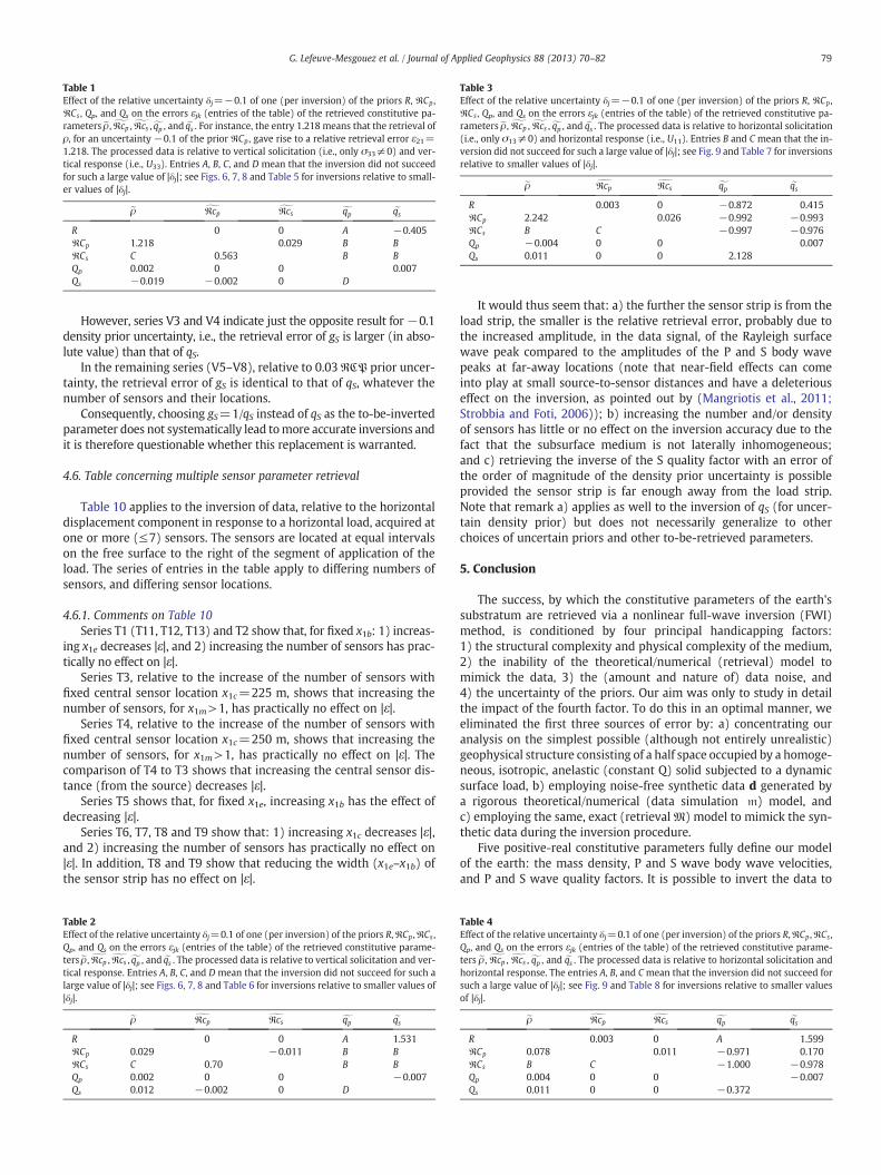
4.4. Tables relative to εjk as a function of δj
Tables 1–4, relative to inversions of data acquired at a single sen-sor located at x1=300 m, show the relative retrieval errors εjk for rel-ative uncertainties δj=±0.1 of the priors. As some of the retrievalsdid not succeed for such large |δj|, |δj| was reduced tenfold, thus givingrise to the results in Tables 5–8.
The index j refers to the row (prior type) and the index k refers tothe column (retrieved parameter type) of each array.
08 0.1 0.12 0.14 0.16s)
00 2200 2400 2600 2800 3000r
ncertainty is in the priorRCS and δ3=0.01. First iteration (for a large parameter searcha signal (red curve) and various trial response curves (blue curves). Bottom panel: costibits no authentic minimum in S, but the shape of the curve suggests that a minimume reader is referred to the web version of this article.)
Fig. 4. Inversion of U33, acquired at one sensor located at x1=300 m, to retrieve ρ when the uncertainty is in the prior RCS and δ3=0.01. Third iteration (for a shifted, smaller pa-rameter search space S such that r=(2900 kg/m3, 3900 kg/m3,6)) in the inversion process for the retrieval of ρ. Top panel: data signal (red curve) and various trial response curves(blue curves). Bottom panel: cost functional K corresponding to the responses for the various trial values of ρ. Note that K begins to exhibit a parabolic shape, with a suggestion thatthe authentic minimum will occur for smaller ρ. (For interpretation of the references to color in this figure legend, the reader is referred to the web version of this article.)
77G. Lefeuve-Mesgouez et al. / Journal of Applied Geophysics 88 (2013) 70–82
4.4.1. Comments on the tables relative to the retrieval errors resultingfrom the prior uncertainties and a single sensor
Tables 1–4 pertain to reasonably-small prior errors δj=±0.1. Fourtypes of retrieval results can be observed in these tables: 1) for some jkcombinations, εjk is of one order of magnitude smaller than |δj| or identi-cally nil, 2) for other jk combinations, εjk is of the order ofmagnitude of δj,
0 0.02 0.04 0.06 0−5
0
5x 10⁻¹²
U
2950 2960 2970 2980 2990 30.1729
0.173
0.1731
0.1732
0.1733
0.1734
0.1735
cost
Fig. 5. Inversion of U33, acquired at one sensor located at x1=300 m, to retrieve ρ when thparameter search space S such that r=(2950 kg/m3, 3050 kg/m3,6)) in the inversion proccurves (blue curves). Bottom panel: cost functional K corresponding to the responses for thvalue of eρ and turns out to be equal to 3010 kg/m3 instead of its target value ρ=2750 kg/mten times the relative uncertainty of the prior. (For interpretation of the references to color
3) for yet other jk combinations, εjk is one order of magnitude greaterthan δj, 4) for a relatively-large number of jk combinations (cases A, B,C, D), it was not possible to carry out the inversion to completion.
For situation 4), it was decided to see what happens when |δj| isreduced by one order of magnitude. This gave rise to the results inTables 5–8 wherein it can be observed that some jk combinations
.08 0.1 0.12 0.14 0.16t(s)
000 3010 3020 3030 3040 3050r
e uncertainty is in the prior RCS and δ3=0.01. Fifth and final iteration (for a smalleress for the retrieval of ρ. Top panel: data signal (red curve) and various trial responsee various trial values of ρ. The location of the minimum of the parabolic K is the final3. This difference corresponds to a relative retrieval error ε31=0.095 which is almostin this figure legend, the reader is referred to the web version of this article.)
Fig. 6. Inversion of signal data relating to U33 acquired at a single sensor located at x1=300 m. Graph of ε14 versus δ1 relative to the retrieval of qP for prior error relating to R.
Fig. 8. Inversion of signal data relating to U33 acquired at a single sensor located at x1=300 m. Graph of ε54 versus δ5 relative to the retrieval of qP for prior error relating to QS.
78 G. Lefeuve-Mesgouez et al. / Journal of Applied Geophysics 88 (2013) 70–82
are really pathological in that they lead to εjk which are two orders ofmagnitude greater than |δj|.
These observations transcend the choices of load and response polar-izations. We shall see in Section 4.6 that the employment of multi-offsetdata does not improve the situation (for fixed central location of the sen-sor group)when the latter is already unsatisfactory formono-offset data.
A last remark: a table such as the ones presented herein hasappeared previously in (De Barros et al., 2010) relative to the retrievalof the constitutive parameters of a porous medium, but in this article,apparently no εjk exceeds approximately 0.4 for the δj=+0.01, a factthat is at odds with our own results; we write ‘apparently’ becausethe entries in the matrix δj=+0.01 of (De Barros et al., 2010), are notnumerical, but rather shades of gray (from white to black) spots, witha colormap which indicates that the black spots could mean that thecorresponding εjk is equal or greater, or even much greater than 0.4.
4.5. Table of the comparison of the accuracies of retrieval of a parameterwith that of its inverse
Due to the difficulty of obtaining accurate retrievals of the P and Squality factors in the presence of prior uncertainty, the questionarises as to whether a different choice of to-be-retrieved parameters,related in some (known) way to qP and qS, might yield more accurate
Fig. 7. Inversion of signal data relating to U33 acquired at a single sensor located at x1=300 m. Graph of ε15 versus δ1 relative to the retrieval of qS for prior error relating to R.
retrievals. This issue, first discussed by (Tarantola, 1986), was statedby this author to be related to what he and others (De Barros andDietrich, 2008) term the parameter coupling problem. For instance,the retrieval of density (ρ) and Lamé parameters (μ, λ) from P- andS-wave velocity (cP, cS respectively) data can lead to difficultiessince ρ and μ are both involved in cS via cS ¼
ffiffiffiffiffiffiffiffiμ=ρ
p, whereas ρ, λ
and μ are all involved in cP via cP ¼ffiffiffiffiffiffiffiffiffiffiffiffiffiffiffiffiffiffiffiffiffiffiffiffiλþ 2μð Þ=ρ
p. A more natural
choice would seem to be to invert for ρ, cP and cS, but Tarantola writesthat his numerical experiments show that a better choice ofto-be-retrieved parameters is ρ, and the two impedances ρcP, ρcS.
Inspired by this remark (but not to the point of inverting forρRcP;Sinstead of RcP;S), we compared retrievals of gS :=1/qS to those of qSusing the same type of data as before, i.e., horizontal displacementin response to a horizontal transient load. The results of this compar-ison are given in Table 10, wherein the prior is either density orP-body wave velocity affected by various uncertainties δ and thedata is acquired at one or three sensors at various locations.
4.5.1. Comments on Table 9Series V1 and V2 indicate that the retrieval error of gS is consider-
ably smaller (in absolute value) than that of qS for 0.1 density prioruncertainty, whatever the number of sensors and their locations.
−0.04 −0.02 0 0.02 0.04 0.06 0.08 0.1−0.2
−0.1
0
0.1
0.2
0.3
0.4
0.5
del(Csr)
eps(
cpr)
Fig. 9. Inversion of signal data relating to U11 acquired at a single sensor located at x1=300 m. Graph of ε32 versus δ3 relative to the retrieval ofRcP for prior error relating toRCS .
Table 1Effect of the relative uncertainty δj=−0.1 of one (per inversion) of the priors R, RCp ,RCs , Qp, and Qs on the errors εjk (entries of the table) of the retrieved constitutive pa-rameters eρ , gRcp ,gRcs ,fqp , and eqs . For instance, the entry 1.218 means that the retrieval ofρ, for an uncertainty −0.1 of the prior RCp , gave rise to a relative retrieval error ε21=1.218. The processed data is relative to vertical solicitation (i.e., only σ33≠0) and ver-tical response (i.e., U33). Entries A, B, C, and D mean that the inversion did not succeedfor such a large value of |δj|; see Figs. 6, 7, 8 and Table 5 for inversions relative to small-er values of |δj|.
eρ gRcp gRcs fqp eqsR 0 0 A −0.405RCp 1.218 0.029 B BRCs C 0.563 B BQp 0.002 0 0 0.007Qs −0.019 −0.002 0 D
Table 3Effect of the relative uncertainty δj=−0.1 of one (per inversion) of the priors R, RCp ,RCs , Qp, and Qs on the errors εjk (entries of the table) of the retrieved constitutive pa-rameters eρ , gRcp , gRcs ,fqp , and eqs . The processed data is relative to horizontal solicitation(i.e., only σ13≠0) and horizontal response (i.e., U11). Entries B and C mean that the in-version did not succeed for such a large value of |δj|; see Fig. 9 and Table 7 for inversionsrelative to smaller values of |δj|.
79G. Lefeuve-Mesgouez et al. / Journal of Applied Geophysics 88 (2013) 70–82
However, series V3 and V4 indicate just the opposite result for −0.1density prior uncertainty, i.e., the retrieval error of gS is larger (in abso-lute value) than that of qS.
In the remaining series (V5–V8), relative to 0.03RCP prior uncer-tainty, the retrieval error of gS is identical to that of qS, whatever thenumber of sensors and their locations.
Consequently, choosing gS=1/qS instead of qS as the to-be-invertedparameter does not systematically lead tomore accurate inversions andit is therefore questionable whether this replacement is warranted.
Table 10 applies to the inversion of data, relative to the horizontaldisplacement component in response to a horizontal load, acquired atone or more (≤7) sensors. The sensors are located at equal intervalson the free surface to the right of the segment of application of theload. The series of entries in the table apply to differing numbers ofsensors, and differing sensor locations.
4.6.1. Comments on Table 10Series T1 (T11, T12, T13) and T2 show that, for fixed x1b: 1) increas-
ing x1e decreases |ε|, and 2) increasing the number of sensors has prac-tically no effect on |ε|.
Series T3, relative to the increase of the number of sensors withfixed central sensor location x1c=225 m, shows that increasing thenumber of sensors, for x1m>1, has practically no effect on |ε|.
Series T4, relative to the increase of the number of sensors withfixed central sensor location x1c=250 m, shows that increasing thenumber of sensors, for x1m>1, has practically no effect on |ε|. Thecomparison of T4 to T3 shows that increasing the central sensor dis-tance (from the source) decreases |ε|.
Series T5 shows that, for fixed x1e, increasing x1b has the effect ofdecreasing |ε|.
Series T6, T7, T8 and T9 show that: 1) increasing x1c decreases |ε|,and 2) increasing the number of sensors has practically no effect on|ε|. In addition, T8 and T9 show that reducing the width (x1e–x1b) ofthe sensor strip has no effect on |ε|.
Table 2Effect of the relative uncertainty δj=0.1 of one (per inversion) of the priors R,RCp ,RCs ,Qp, and Qs on the errors εjk (entries of the table) of the retrieved constitutive parame-ters eρ , gRcp ,gRcs ,fqp , and eqs . The processed data is relative to vertical solicitation and ver-tical response. Entries A, B, C, and D mean that the inversion did not succeed for such alarge value of |δj|; see Figs. 6, 7, 8 and Table 6 for inversions relative to smaller values of|δj|.
eρ gRcp gRcs fqp eqsR 0 0 A 1.531RCp 0.029 −0.011 B BRCs C 0.70 B BQp 0.002 0 0 −0.007Qs 0.012 −0.002 0 D
It would thus seem that: a) the further the sensor strip is from theload strip, the smaller is the relative retrieval error, probably due tothe increased amplitude, in the data signal, of the Rayleigh surfacewave peak compared to the amplitudes of the P and S body wavepeaks at far-away locations (note that near-field effects can comeinto play at small source-to-sensor distances and have a deleteriouseffect on the inversion, as pointed out by (Mangriotis et al., 2011;Strobbia and Foti, 2006)); b) increasing the number and/or densityof sensors has little or no effect on the inversion accuracy due to thefact that the subsurface medium is not laterally inhomogeneous;and c) retrieving the inverse of the S quality factor with an error ofthe order of magnitude of the density prior uncertainty is possibleprovided the sensor strip is far enough away from the load strip.Note that remark a) applies as well to the inversion of qS (for uncer-tain density prior) but does not necessarily generalize to otherchoices of uncertain priors and other to-be-retrieved parameters.
5. Conclusion
The success, by which the constitutive parameters of the earth'ssubstratum are retrieved via a nonlinear full-wave inversion (FWI)method, is conditioned by four principal handicapping factors:1) the structural complexity and physical complexity of the medium,2) the inability of the theoretical/numerical (retrieval) model tomimick the data, 3) the (amount and nature of) data noise, and4) the uncertainty of the priors. Our aim was only to study in detailthe impact of the fourth factor. To do this in an optimal manner, weeliminated the first three sources of error by: a) concentrating ouranalysis on the simplest possible (although not entirely unrealistic)geophysical structure consisting of a half space occupied by a homoge-neous, isotropic, anelastic (constant Q) solid subjected to a dynamicsurface load, b) employing noise-free synthetic data d generated bya rigorous theoretical/numerical (data simulation m) model, andc) employing the same, exact (retrievalM) model to mimick the syn-thetic data during the inversion procedure.
Five positive-real constitutive parameters fully define our modelof the earth: the mass density, P and S wave body wave velocities,and P and S wave quality factors. It is possible to invert the data to
Table 4Effect of the relative uncertainty δj=0.1 of one (per inversion) of the priors R,RCp ,RCs ,Qp, and Qs on the errors εjk (entries of the table) of the retrieved constitutive parame-ters eρ , gRcp , gRcs ,fqp , and eqs . The processed data is relative to horizontal solicitation andhorizontal response. The entries A, B, and Cmean that the inversion did not succeed forsuch a large value of |δj|; see Fig. 9 and Table 8 for inversions relative to smaller valuesof |δj|.
eρ gRcp gRcs fqp eqsR 0.003 0 A 1.599RCp 0.078 0.011 −0.971 0.170RCs B C −1.000 −0.978Qp 0.004 0 0 −0.007Qs 0.011 0 0 −0.372
Table 5Effect of the relative uncertainty δj=−0.01 of one (per inversion) of the priorsRCp
andRCs on the errors εjk (entries of the table) of the retrieved constitutive param-eters fqp and eqs . The processed data is relative to vertical solicitation and verticalresponse.
fqp eqsRCp −0.265 0.116RCs −0.813 −0.442
Table 7Effect of the relative uncertainty δj=−0.01 of one (per inversion) of the priorsRCp
andRCs on the errors εjk (entries of the table) of the retrieved constitutive param-eters fqp and eqs . The processed data is relative to horizontal solicitation and hori-zontal response.
fqp eqsRCp −0.412 −0.177RCs −1.000 −0.422
80 G. Lefeuve-Mesgouez et al. / Journal of Applied Geophysics 88 (2013) 70–82
obtain all five parameters at one time, but this procedure can be verycostly in terms of computation time especially if the values of thesought-for parameters are not well-known a priori (which requiresa very large five-dimensional initial parameter search space) and isnot guaranteed to succeed because the sensitivities of the data to var-iations of the parameters varies from one parameter to the other. An-other approach (the one adopted herein) is to divide the fullparameter set p into two subsets: the set r of parameters one wantsto retrieve by the inversion scheme, and the set q of parameters(priors) that are considered to be known a priori. The word ‘known’here means ‘not to be retrieved’, but certainly does not mean ‘perfect-ly well-known’. In fact, whether the value of a prior is obtained by amore-or-less educated guess, or by some experimental measurementor simulation scheme other than the one employed to obtain d, it issubject to a certain degree of uncertainty. We attributed the symbolδj to the relative uncertainty of the j-th prior and sought to quantify,one after another and one at a time, the effect of each of the five pos-sible prior uncertainties on the relative retrieval error εjk of the k-thto-be-retrieved parameter (amongst the remaining four parameters).Thus, each εjk is the result of an inversion procedure which seeks toretrieve a single parameter at a time, assuming that amongst thefour other parameters, three are perfectly-well known, and thevalue of the last parameter is uncertain.
We could, of course, have performed computations for inversionsof: 1) one parameter at a time, assuming that two (three) of the priorsare perfectly-well known and the value of the other two (one) pa-rameters are uncertain, 2) two, three, four parameters at a timewith a variable number of uncertain priors, but the great number ofresults of such interesting studies cannot be accounted-for in a singlepublication such as the present one. Furthermore, the present paperled to results which show that the other inversion strategies are liableto lead to difficulties that will probably be aggravated if more thanone parameter is sought-for at a time and/or more than one prior isaffected by uncertainty during a given inversion.
A word is in order about the meaning of the term ‘inversion’. Inthis paper, inversion meant an iterative process by which the globalminimum of a discrepancy (cost) functional K is sought. K is a mea-sure of the discrepancy between the data signal(s) (the plural apply-ing to multi-offset data) involving the true parameters p=q+r, andthe signal(s) one obtains by the retrieval model involving the param-eters P=Q+R. A search spaceS (actually a segment, since we searchfor a single parameter) is chosen at each step of the inversion and thisspace (segment) is discretized so as to form a grid, the nodes of whichcorrespond to different (trial) values of R (note that Q does notchange from point-to-point of this grid). The set of all the values ofK on this grid is G and at each step of the inversion the algorithm
Table 6Effect of the relative uncertainty δj=0.01 of one (per inversion) of the priors RCp
andRCs on the errors εjk (entries of the table) of the retrieved constitutive param-eters fqp and eqs . The processed data is relative to vertical solicitation and verticalresponse.
fqp eqsRCp −0.225 0.066RCs −0.932 −0.410
selects the point r̃ in G at which K is a minimum. This process wasshown to require a certain number of steps: a) because it is possiblefor no clear-cut minimum to appear for a given choice of S and/orb) in order to attain a prescribed accuracy in the location of the globalminimum of K. Moreover, it was shown that the inversion procedurecannot be carried out in an unsupervised manner when, as was as-sumed herein, the initial knowledge one has of both r and q isvague. This aspect of nonlinear FWI inversion will probably be exacer-bated if the choice is made to invert for more than one parameter at atime.
We consider, perhaps rather arbitrarily, that the retrieval of a given(k-th) parameter is successful with regard to relative uncertainty δj ofthe j-th prior, if the relative retrieval error εjk is of the order of, or oforder less than, δj. Our numerical trials first concerned a very reasonablerelative uncertainty of 0.1 (note that in (De Barros et al., 2010), this was0.01, a value which appears to us to be unattainable in real-life). Fortu-nately, we found that:
a the retrievals of the density generally succeed well and are insen-sitive to most varieties of prior errors;
b the retrievals of the (real part of) P body wave velocity generallysucceed well and are insensitive to most varieties of prior errors:
c the retrievals of the (real part of) S body wave velocity succeedwell and are insensitive to all varieties of prior errors.
Surprisingly, we found that it was impossible to retrieve severalparameters (principally the quality factors) for this level of uncertain-ty of the priors. Moreover, the relative retrieval error of the density,for 0.1 relative error of the (real part of) body wave velocities, wasfound to attain the anomalous values of between ten and twentytimes δj, and similar anomalies (although of lesser amplitude) werefound for the retrieval of the (real part of) P body wave velocitywhen the uncertainty of the (real part of) S body wave velocityprior was δj=0.1. This incited us to revise our appreciation of whatconstitutes a ‘reasonable’ amount of relative prior uncertainty, morein line with De Barros et al. (2010). Consequently, we implementedhis revision by carrying out the inversions in the anomalous casesfor δj=0.05,0.03,…,0.01. This led, once again, to surprising results,such as a retrieval error concerning the (real part of) S body wave ve-locity which attains one hundred times the relative prior uncertaintyof the (real part of) P body wave velocity.
We sought to improve the retrievals via variations of the natureand quantity of the data, by: a) changing the polarization (verticalto horizontal) of the load and the field component (vertical to hori-zontal), and b) increasing the number of receivers, but these mea-sures did not significantly change the anomalous results. We alsotried to improve the accuracy of the retrieval of the S quality factor
Table 8Effect of the relative uncertainty δj=0.01 of one (per inversion) of the priorsRCp andRCs on the errors εjk (entries of the table) of the retrieved constitutive parametersfqpand eqs . The processed data is relative to horizontal solicitation and horizontalresponse.
fqp eqsRCp −0.372 0.190RCs −0.914 −0.422
Table 9Retrieval error (ε) of the inverse shear quality factor gS=1/qS compared to that of theshear quality factor qS for various prior uncertainties δ of either the density (R) or thelongitudinal body wave velocity (RCp). The processed data is relative to horizontal so-licitation and horizontal response. Effect of the variation of the number and positions ofthe sensors. The symbols x1b, x1e, x1m denote the left-most abscissa (in meters),right-most abscissa (in meters), and the number (odd and ≥1) respectively of sensorson the ground.
81G. Lefeuve-Mesgouez et al. / Journal of Applied Geophysics 88 (2013) 70–82
by instead inverting for its inverse, but this did not systematicallylead to the hoped-for improvement. We did not evaluate the effectof processing windowed data signals, which in certain limits,
Table 10Retrieval error (ε) of the inverse shear quality factor gS=1/qSwhen the uncertainty δ of thedensity (R) prior is =0.1 and the processed data is relative to horizontal solicitation andhorizontal response. Effect of the variation of the number and positions of the sensors.The symbols x1b, x1e, x1m denote the left-most abscissa (in meters), right-most abscissa(in meters), and the number (odd and ≥1) respectively of sensors on the ground. The(constant) interval between successive receivers is δx1=(x1e−x1b)/(x1m−1); m=3,5,…and the position of the central sensor is x1c=(x1e+x1b)/2.
Reference Q r (x1b, x1e, x1m) δ ε Comment
T11 R gS (150,200,3) 0.1 −0.9412 x1b=150 constantT12 R gS (150,300,3) 0.1 −0.77303 δx1 increasingT13 R gS (150,350,3) 0.1 −0.6766 3 sensors
T21 R gS (150,200,5) 0.1 −0.9412 x1b constantT22 R gS (150,300,5) 0.1 −0.7795 δx1 increasingT23 R gS (150,350,5) 0.1 −0.69277 5 sensors
T31 R gS (225,225,1) 0.1 −0.82066 x1c=225 constantT32 R gS (150,300,3) 0.1 −0.77303 δx1 decreasingT33 R gS (150,300,5) 0.1 −0.7795 1, 3, 5, 7 sensorsT34 R gS (150,300,7) 0.1 −0.7942
T41 R gS (250,250,1) 0.1 −0.7354 x1c=250 constantT42 R gS (150,350,3) 0.1 −0.6766 δx1 decreasingT43 R gS (150,350,5) 0.1 −0.68983 1, 3, 5 ,7 sensorsT44 R gS (150,350,7) 0.1 −0.69424
T51 R gS (100,350,5) 0.1 −0.7207 x1e=350 constantT52 R gS (150,350,5) 0.1 −0.68983 δx1 decreasingT53 R gS (200,350,5) 0.1 −0.65014 5 sensors
T61 R gS (325,325,1) 0.1 −0.559 x1c=325 constantT62 R gS (250,400,3) 0.1 −0.559 δx1 decreasingT63 R gS (250,400,7) 0.1 −0.559 1, 3, 7 sensors
T71 R gS (400,400,1) 0.1 −0.4708 x1c=400 constantT72 R gS (325,475,3) 0.1 −0.4561 δx1 decreasingT73 R gS (325,475,5) 0.1 −0.4561 1, 3, 5 sensors
T81 R gS (700,700,1) 0.1 −0.265 x1c=700 constantT82 R gS (600,800,3) 0.1 −0.265 δx1 decreasingT83 R gS (600,800,5) 0.1 −0.265 1, 3, 5, 7 sensorsT84 R gS (600,800,7) 0.1 −0.265 x1b=600, x1e=800T91 R gS (700,700,1) 0.1 −0.265 x1c=700 constant
T92 R gS (650,750,3) 0.1 −0.265 δx1 decreasingT93 R gS (650,750,5) 0.1 −0.265 1, 3, 5, 7 sensorsT94 R gS (650,750,7) 0.1 −0.265 x1b=650, x1e=750
amounts to travel-time data processing, but this is certainly an inter-esting option for future research.
We showed that when the Rayleigh surface wave dominates thesignal (as for large source-sensor distances), the retrieval error (ofthe inverse of the S-quality factor for uncertain density prior) isless than that at small source-sensor distances. We found the sameto be true when the to-be-retrieved parameter is the S-quality factor(for uncertain density prior), but did not seek to determine whetherthis rule generalizes to other prior/to-be-retrieved parametercombinations. This question will be treated in depth in a futurepublication.
In several examples, we observed that the trial response curvecorresponding to the final retrieved value of a parameter, was quite‘close’ to the true data curve despite the fact that the retrieved param-eter was quite different from its true value. This implies that visual‘closeness’ of these two curves should not be taken as a foolproof in-dication of a small relative retrieval error.
It goes without saying that no general rules can be deduced fromthe results presented herein; however, our study should incite allthose who undertake parameter retrievals (particularly by means ofnonlinear full-wave schemes, and in more complex structuralmodels) of the earth's substratum to be very cautious about the sig-nificance of their findings due to the fact that prior uncertainty canlead to unforeseeable retrieval errors.
A generalization of this study is underway for medium parameterretrieval and source parameter retrieval in layered anelastic/poroelastichalf space models of the earth.
References
Achenbach, J.D., 1973. Wave Propagation in Elastic Solids. North-Holland, Amsterdam.Aki, K., Richards, P.G., 1980. Quantitative Seismology, Theory andMethods, Vol. II. Freeman,
New York.Amoruso, A., Crescentini, L., Fidani, C., 2004. Effects of crustal layering on source pa-
rameter inversion from coseismic geodetic data. Geophysical Journal International159, 353–364.
Aoi, S., Iwata, T., Irikura, K., Sanchez-Sesma, F.J., 1995. Waveform inversion for deter-mining the boundary shape of a basin structure. The Bulletin of the SeismologicalSociety of America 85, 1445–1455.
Bard, P.-Y., Tucker, B.E., 1985. Underground and ridge site effects: a comparison of ob-servation and theory. The Bulletin of the Seismological Society of America 75,905–922.
Bodet L., 2005. Limites théoriques et expérimentales de l'interprétation de la disper-sion des ondes de Rayleigh: apport de la modélisation numérique et physique,Thesis, Université de Nantes, Nantes.
Boore, D.M., 1972. A note on the effect of simple topography on seismic SH waves. TheBulletin of the Seismological Society of America 62, 275–284.
Bouchon,M., 1973. Effect of topography on surfacemotion. The Bulletin of the SeismologicalSociety of America 63, 615–632.
Bouchon, M., 1981. A simple method to calculate Green's functions in elastic layeredmedia, 71, pp. 959–979.
Buchanan, J.L., Gilbert, R.P., Wirgin, A., Xu, Y., 2000. Identification, by the intersectingcanonical domain method, of the size, shape and depth of a soft body of revolutionlocated within an acoustic waveguide. Inverse Problems 16, 1709–1726.
Buchanan, J.L., Gilbert, R.P., Wirgin, A., Xu, Y., 2002. Depth sounding: an illustration ofsome of the pitfalls of inverse scattering problems. Mathematical and ComputerModelling 35, 1315–1354.
Buchanan, J.L., Gilbert, R.P., Ou, M.-J.Y., 2011. Recovery of the parameters of cancellousbone by inversion of effective velocities, and transmission and reflection coeffi-cients. Inverse Problems 27, 125006 http://dx.doi.org/10.1088/0266-5611/27/12/125006.
Burstedde, C., Ghattas, O., 2009. Algorithmic strategies for full waveform inversion: 1Dexperiments. Geophysics 74, WCC37–WCC46.
Chotiros, N.P., 2002. An inversion for Biot parameters in water-saturated sand. TheJournal of the Acoustical Society of America 112, 1853–1868.
Colton, D., Kress, R., 1992. Inverse Acoustic and Electromagnetic Scattering Theory.Springer, Berlin.
Cox H.L.H., 1991. Estimation of macro velocity models by wave field extrapolation,Ph.D. thesis, Technische Universiteit Delft, Delft.
Curtis, A., Lomax, A., 2001. Prior information, sampling distributions and the curse ofdimensionality. Geophysics 66, 372–378.
De Barros, L., Dietrich, M., 2008. Perturbations of the seismic reflectivity of a fluid-saturated depth-dependent poroelastic medium. The Journal of the AcousticalSociety of America 123, 1409–1420.
De Barros, L., Dietrich, M., Valette, B., 2010. Full waveform inversion of seismic wavesreflected in a stratified porous medium. Geophysical Journal International 182,1543–1556.
82 G. Lefeuve-Mesgouez et al. / Journal of Applied Geophysics 88 (2013) 70–82
Delprat-Jannaud, F., Lailly, P., 2005. A fundamental limitation for the reconstruction ofimpedance profiles from seismic data. Geophysics 70, R1–R14.
Dessa, J.-X., Pascal, G., 2003. Combined traveltime and frequency-domain seismicwaveform inversion: a case study on multi-offset ultrasonic data. GeophysicalJournal International 154, 117–133.
Dupuy B., 2011. Propagation des ondes sismiques dans les milieux multiphasiqueshétérogènes: modélisation numérique, sensibilité et inversion des paramètresporoélastiques, Thesis, Université de Grenoble, Grenoble.
Eringen, A.C., Suhubi, E., 1975. Elastodynamics. Linear Theory, vol. 2. Academic Press,New York, pp. 614–629.
Fäh, D., Suhadolc, P., Mueller, S., Panza, G.F., 1994. A hybrid method for the estimationof ground motion in sedimentary basins: quantitative modeling for Mexico City.The Bulletin of the Seismological Society of America 84, 383–399.
Feigl, K.L., 2002. Estimating earthquake source parameters from geodetic measurements.International Handbook of Earthquake and Engineering Seismology, vol. 81A. Elsevier,Amsterdam, pp. 1–15. ch. 37.
Forbriger, T., 2003. Inversion of shallow-seismic wavefields: II. Inferring subsurface prop-erties from wavefield transforms. Geophysical Journal International 153, 735–752.
Foti, S., Comina, C., Boiero, D., Socco, L.V., 2009. Non-uniqueness in surface-wave inversionand consequences on seismic site response analyses. Soil Dynamics and EarthquakeEngineering 29, 982–993.
Geli, L., Bard, P.-Y., Jullien, B., 1988. The effect of topography on earthquake groundmotion: areview and new results. The Bulletin of the Seismological Society of America 78, 42–63.
Gelis C., 2005. Inversion des formes d'onde élastique dans le domaine espace-fréquence en deux dimensions. Application à la caractérisation de la subsurfacedans le cadre de la détection de cavités souterraines, Ph.D. thesis, Université deNice Sophia-Antipolis, Nice.
Gelis, C., Virieux, J., Grandjean, G., 2007. Two-dimensional elastic full waveform inver-sion using Born and Rytov formulations in the frequency domain. GeophysicalJournal International 168, 605–633.
Goldman, M., Mogilatov, V., Rabinovich, M., 1996. Transient response of a homoge-neous half space with due regard for displacement currents. Journal of AppliedGeophysics 34, 291–305.
Groby J.-P., 2005. Modélisation de la propagation des ondes élastiques générées par unséisme proche ou éloigné à l'intérieur d'une ville, Ph.D. thesis, Université Aix-MarseilleII, Marseille.
Groby, J.-P., Wirgin, A., 2005. Two-dimensional ground motion at a soft viscoelasticlayer/hard substratum site in response to SH cylindrical seismic waves radiatedby deep and shallow line sources-I. Theory. Geophysical Journal International163, 165–191.
Groby, J.-P., Ogam, E., Wirgin, A., Xu, Y., 2011. Recovery of a material parameter of a softelastic layer. Complex Variables and Elliptic Equations 56, 3001–3020.
Hurley, D.H., Spicer, J.B., 2004. Line source representation for laser-generated ultra-sound in an elastic transversely isotropic half-space. The Journal of the AcousticalSociety of America 116, 2914–2922.
Jeong, W., Lee, H.-Y., Min, D.-J., 2012. Full waveform inversion strategy for density inthe frequency domain. Geophysical Journal International 188, 1221–1242.
Kawase, H., Aki, K., 1989. A study on the response of a soft basin for incident S, P, andRayleigh waves with special reference to the long duration observed in MexicoCity. The Bulletin of the Seismological Society of America 79, 1361–1382.
Kennett, B.L.N., 2001. The Seismic Wavefield. Cambridge University Press, Cambridge.Kolb, P., Collino, F., Lailly, P., 1986. Pre-stack inversion of a 1-D medium. Proceedings of
the IEEE 74, 498–508.Korenaga, J., Holbrook, W.S., Singh, S.C., Minshull, T.A., 1997. Natural gas hydrates on the
southeast U.S. margin: constraints from full waveform and travel time inversions ofwide-angle seismic data. Journal of Geophysical Research B7 (102), 15345–15365.
Kormendi, F., Dietrich, M., 1991. Nonlinear waveform inversion of plane-waveseismograms in stratified elastic media. Geophysics 56, 664–674.
Kozhevnikov, N.O., Antonov, E.Y., 2008. Inversion of TEM data affected by fast-decayinginduced polarization: Numerical simulation experiment with homogeneous half-space. Journal of Applied Geophysics 66, 31–43.
Liu, H.-P., Anderson, D.L., Kanamori, H., 1976. Velocity dispersion due to anelasticity;implications for seismology and mantle composition. Geophysical Journal of theRoyal Astronomical Society 47, 41–58.
Mangriotis, M.-D., Rector, J.W., Herkenhoff, E.F., 2011. Case history — effects of thenear-field on shallow seismic studies. Geophysics 76, B9–B18.
Mesgouez A., 2005. Etude numérique de la propagation des ondes mécaniques dans unmilieu poreux en régime impulsionnel, Ph.D. thesis, Université d'Avignon et despays de Vaucluse, Avignon.
Mora, P., 1987. Nonlinear two-dimensional elastic inversion of multioffset seismic data.Geophysics 52, 1211–1228.
Muijs, R., Holliger, K., Robertsson, O.A., 2002. Perturbation analysis of an explicitwavefield separation scheme for P- and S-waves. Geophysics 67, 1972–1982.
Ogam, E., Scotti, T., Wirgin, A., 2001. Non-ambiguous boundary identification of a cylindri-cal object by acoustic waves. Comptes Rendus de l'Académie des Sciences— Series IIB239, 61–66.
Ogam, E., Scotti, T., Wirgin, A., 2002. Non-uniqueness in connection with methods forthe reconstruction of the shape of cylindrical bodies from acoustic scattering data.In: Wirgin, A. (Ed.), Acoustics, Mechanics and the Related Topics of MathematicalAnalysis. World Scientific, Singapore, pp. 222–228.
Okada, Y., 1985. Surface deformation due to shear and tensile faults in a half space. TheBulletin of the Seismological Society of America 75, 1135–1154.
Operto, S., Ravaut, C., Improta, L., Virieux, J., Herrero, A., 2004. Quantitative imaging ofcomplex structures from dense wide-aperture seismic data by multiscaletraveltime and waveform inversions; a case study. Geophysical Prospecting 52,625–651.
Pereyra, V., Keller, H.B., Lee, W.H.K., 1980. Computational methods for inverse prob-lems in geophysics: inversion of travel time observations. Physics of the Earthand Planetary Interiors 21, 120–125.
Pratt, G., 1999. Seismic waveform inversion in the frequency domain, Part 1; theoryand verification in a physical scale model. Geophysics 64, 888–901.
Rayleigh, L., 1885. On waves propagated along the surface of an elastic solid. Proceedingsof the London Mathematical Society 17, 4–11.
Ribodetti, A., Virieux, J., 1998. Asymptotic theory for imaging the attenuation factor Q.Geophysics 63, 1767–1778.
Robertsson, J.O.A., 1996. A numerical free-surface condition for elastic/viscoelastic finite-difference modeling in the presence of topography. Geophysics 61, 1921–1934.
Sacks, P., Symes, W., 1987. Recovery of the elastic parameters of a layered half-space.Geophysical Journal of the Royal Astronomical Society 88, 593–620.
Scales, J.A., Tenorioz, L., 2001. Prior information and uncertainty in inverse problems.Geophysics 66, 389–397.
Scotti, T., Wirgin, A., 1995. Shape reconstruction using diffracted waves and canonicalsolutions. Inverse Problems 11, 1097–1111.
Scotti, T., Wirgin, A., 2004. Reconstruction of the three mechanical material constantsof a lossy fluid-like cylinder from low-frequency scattered acoustic fields. ComptesRendus Mécanique 332, 717–724.
Sebaa, N., Fellah, Z.E.A., Fellah,M., Ogam, E.,Wirgin, A., Mitri, F.G., Depollier, C., Lauriks,W.,2006. Ultrasonic characterization of human cancellous bone using the Biot theory:Inverse problem. The Journal of the Acoustical Society of America 120, 1816–1824.
Song, Z.M., Williamson, P.R., Pratt, R.G., 1995. Frequency-domain acoustic-wavemodeling and inversion of crosshole data: Part II — inversion method, syntheticexperiments and real-data results. Geophysics 60, 796–809.
Strobbia, C., Foti, S., 2006. Multi-offset phase analysis of surface wave data (MOPA).Journal of Applied Geophysics 59, 300–313.
Sun, R., McMechan, G.A., 1992. Full-wavefield inversion for wide-aperture, elastic,seismic data. Geophysical Journal International 111, 1–10.
Tarantola, A., 1984. Inversion of seismic data in the acoustic approximation. Geophysics49, 1259–1266.
Tarantola, A., 1986. A strategy for nonlinear elastic inversion of seismic reflection data.Geophysics 51, 1893–1903.
Van der Made P.M., 1988. Determination of macro subsurface models by generalizedinversion, Ph.D thesis, Technische Universiteit Delft, Delft.
Van Vossen, R., Trampert, J., Curtis, A., 2004. Propagator and wave-equation inversionfor near-receiver material properties. Geophysical Journal International 157,796–812.
Virieux, J., Operto, S., 2009. An overview of full-waveform inversion in exploration geo-physics. Geophysics 74, WCC127–WCC152.
Wirgin, A., 2004. The inverse crime. http://arxiv.org/abs/math-ph/0401050.Wirgin, A., Scotti, T., 1996. Wide-band approximation of the sound field scattered by an
impenetrable body. Journal of Sound and Vibration 194, 537–572.Wu, G.R., Zhong, W.F., Dai, H., 2001. Nonlinear inversion of strong scatterer of elastic
wave for two parameters in half-space, Acta Mech. Solida Sinica 14, 235–241.Xia, J., Miller, R.D., Park, C.B., 1999. Estimation of near-surface shear-wave velocity by
inversion of Rayleigh waves. Geophysics 64, 691–700.Xu, P.-C., Mal, A.K., 1987. Calculation of the inplane Green's functions for a layered vis-
coelastic solid. The Bulletin of the Seismological Society of America 77, 1823–1837.