110
www.retscreen.net International RETScreen ® Clean Energy Decision Support Centre RETScreen ® Software Online User Manual Wind Energy Project Model

www.retscreen.net
InternationalRETScreen®
Clean Energy Decision Support Centre
RETScreen® Software Online User Manual
Wind Energy Project Model

Background This document allows for a printed version of the RETScreen® Software Online User Manual, which is an integral part of the RETScreen Software. The online user manual is a Help file within the software. The user automatically downloads the online user manual Help file while downloading the RETScreen Software. Reproduction This document may be reproduced in whole or in part in any form for educational or nonprofit uses, without special permission, provided acknowledgment of the source is made. Natural Resources Canada would appreciate receiving a copy of any publication that uses this report as a source. However, some of the materials and elements found in this report are subject to copyrights held by other organizations. In such cases, some restrictions on the reproduction of materials or graphical elements may apply; it may be necessary to seek permission from the author or copyright holder prior to reproduction. To obtain information concerning copyright ownership and restrictions on reproduction, please contact RETScreen International. Disclaimer This report is distributed for informational purposes and does not necessarily reflect the views of the Government of Canada nor constitute and endorsement of any commercial product or person. Neither Canada nor its ministers, officers, employees or agents makes any warranty in respect to this report or assumes any liability arising out of this report. ISBN: 0-662-36820-7 Catalogue no.: M39-104/2004E-PDF © Minister of Natural Resources Canada 1997-2004.
RETScreen® Wind Energy Project Model
TABLE OF CONTENTS Brief Description and Model Flow Chart.....................................................................................4
Wind Energy Project Model..........................................................................................................9
Energy Model................................................................................................................................10
Equipment Data............................................................................................................................21
Cost Analysis.................................................................................................................................25
Financial Summary ......................................................................................................................52
Greenhouse Gas (GHG) Emission Reduction Analysis ............................................................70
Sensitivity and Risk Analysis.......................................................................................................87
Product Data .................................................................................................................................96
Weather Data................................................................................................................................97
Cost Data .......................................................................................................................................98
Training and Support ..................................................................................................................99
Terms of Use ...............................................................................................................................100
Bibliography................................................................................................................................102
Website Addresses......................................................................................................................104
Index ............................................................................................................................................106
WIND.3
RETScreen® Software Online User Manual
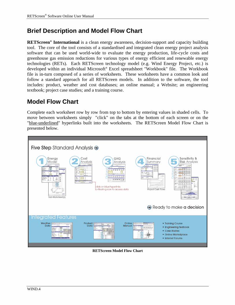
Brief Description and Model Flow Chart RETScreen® International is a clean energy awareness, decision-support and capacity building tool. The core of the tool consists of a standardised and integrated clean energy project analysis software that can be used world-wide to evaluate the energy production, life-cycle costs and greenhouse gas emission reductions for various types of energy efficient and renewable energy technologies (RETs). Each RETScreen technology model (e.g. Wind Energy Project, etc.) is developed within an individual Microsoft® Excel spreadsheet "Workbook" file. The Workbook file is in-turn composed of a series of worksheets. These worksheets have a common look and follow a standard approach for all RETScreen models. In addition to the software, the tool includes: product, weather and cost databases; an online manual; a Website; an engineering textbook; project case studies; and a training course. Model Flow Chart Complete each worksheet row by row from top to bottom by entering values in shaded cells. To move between worksheets simply "click" on the tabs at the bottom of each screen or on the "blue-underlined" hyperlinks built into the worksheets. The RETScreen Model Flow Chart is presented below.
RETScreen Model Flow Chart
WIND.4
RETScreen® Wind Energy Project Model
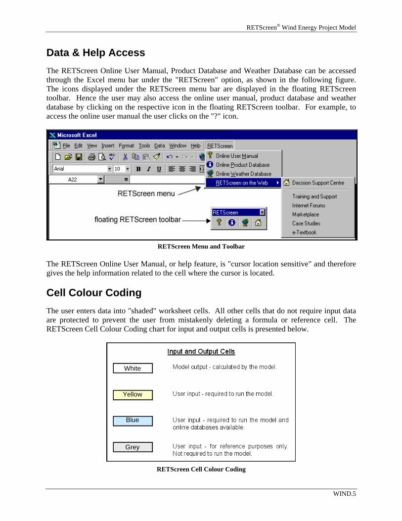
Data & Help Access The RETScreen Online User Manual, Product Database and Weather Database can be accessed through the Excel menu bar under the "RETScreen" option, as shown in the following figure. The icons displayed under the RETScreen menu bar are displayed in the floating RETScreen toolbar. Hence the user may also access the online user manual, product database and weather database by clicking on the respective icon in the floating RETScreen toolbar. For example, to access the online user manual the user clicks on the "?" icon.
RETScreen Menu and Toolbar
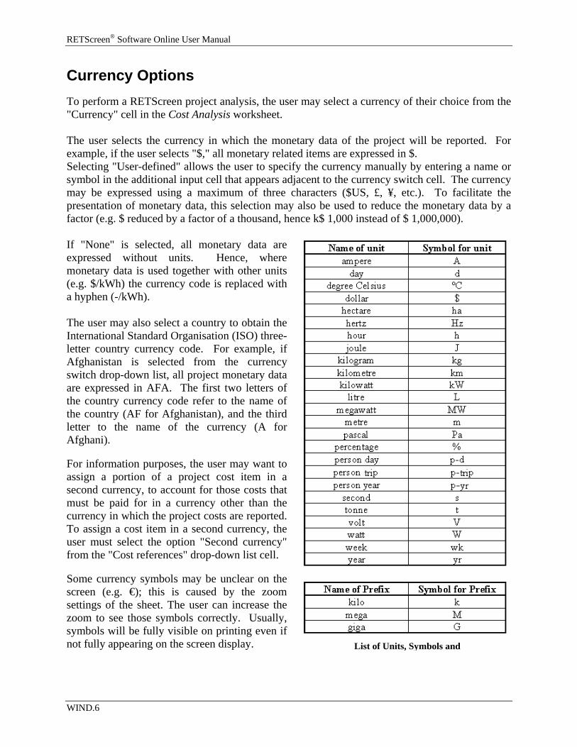
The RETScreen Online User Manual, or help feature, is "cursor location sensitive" and therefore gives the help information related to the cell where the cursor is located. Cell Colour Coding The user enters data into "shaded" worksheet cells. All other cells that do not require input data are protected to prevent the user from mistakenly deleting a formula or reference cell. The RETScreen Cell Colour Coding chart for input and output cells is presented below.
White
Yellow
Blue
Grey
RETScreen Cell Colour Coding
WIND.5
RETScreen® Software Online User Manual
Currency Options To perform a RETScreen project analysis, the user may select a currency of their choice from the "Currency" cell in the Cost Analysis worksheet. The user selects the currency in which the monetary data of the project will be reported. For example, if the user selects "$," all monetary related items are expressed in $. Selecting "User-defined" allows the user to specify the currency manually by entering a name or symbol in the additional input cell that appears adjacent to the currency switch cell. The currency may be expressed using a maximum of three characters ($US, £, ¥, etc.). To facilitate the presentation of monetary data, this selection may also be used to reduce the monetary data by a factor (e.g. $ reduced by a factor of a thousand, hence k$ 1,000 instead of $ 1,000,000). If "None" is selected, all monetary data are expressed without units. Hence, where monetary data is used together with other units (e.g. $/kWh) the currency code is replaced with a hyphen (-/kWh).
List of Units, Symbols and
The user may also select a country to obtain the International Standard Organisation (ISO) three-letter country currency code. For example, if Afghanistan is selected from the currency switch drop-down list, all project monetary data are expressed in AFA. The first two letters of the country currency code refer to the name of the country (AF for Afghanistan), and the third letter to the name of the currency (A for Afghani). For information purposes, the user may want to assign a portion of a project cost item in a second currency, to account for those costs that must be paid for in a currency other than the currency in which the project costs are reported. To assign a cost item in a second currency, the user must select the option "Second currency" from the "Cost references" drop-down list cell. Some currency symbols may be unclear on the screen (e.g. €); this is caused by the zoom settings of the sheet. The user can increase the zoom to see those symbols correctly. Usually, symbols will be fully visible on printing even if not fully appearing on the screen display.
WIND.6
RETScreen® Wind Energy Project Model
Units, Symbols & Prefixes The table above presents a list of units, symbols and prefixes that are used in the RETScreen model. Unit Options To perform a RETScreen project analysis, the user must choose between "Metric" units or "Imperial" units from the "Units" drop down list. If the user selects "Metric," all input and output values will be expressed in metric units. But if the user selects "Imperial," input and output values will be expressed in imperial units where applicable. Only metric units are shown when they are the standard units used by the international wind energy industry (e.g. hub height). Note that if the user switches between "Metric" and "Imperial," input values will not be automatically converted into the equivalent selected units. The user must ensure that values entered in input cells are expressed in the units shown.
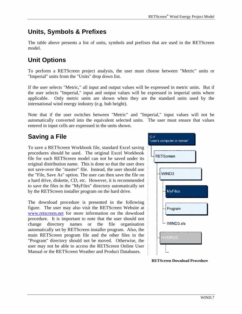
Saving a File To save a RETScreen Workbook file, standard Excel saving procedures should be used. The original Excel Workbook file for each RETScreen model can not be saved under its original distribution name. This is done so that the user does not save-over the "master" file. Instead, the user should use the "File, Save As" option. The user can then save the file on a hard drive, diskette, CD, etc. However, it is recommended to save the files in the "MyFiles" directory automatically set by the RETScreen installer program on the hard drive. The download procedure is presented in the following figure. The user may also visit the RETScreen Website at www.retscreen.net for more information on the download procedure. It is important to note that the user should not change directory names or the file organisation automatically set by RETScreen installer program. Also, the main RETScreen program file and the other files in the "Program" directory should not be moved. Otherwise, the user may not be able to access the RETScreen Online User Manual or the RETScreen Weather and Product Databases.
RETScreen Download Procedure
WIND.7

RETScreen® Software Online User Manual
Printing a File To print a RETScreen Workbook file, standard Excel printing procedures should be used. The workbooks have been formatted for printing the worksheets on standard "letter size" paper with a print quality of 600 dpi. If the printer being used has a different dpi rating then the user must change the print quality dpi rating by selecting "File, Page Setup, Page and Print Quality" and then selecting the proper dpi rating for the printer. Otherwise the user may experience quality problems with the printed worksheets.
WIND.8
RETScreen® Wind Energy Project Model
Wind Energy Project Model The RETScreen® International Wind Energy Project Model can be used world-wide to easily evaluate the energy production, life-cycle costs and greenhouse gas emissions reduction for central-grid, isolated-grid and off-grid wind energy projects, ranging in size from large-scale multi-turbine wind farms to small-scale single-turbine wind-diesel hybrid systems. Six worksheets (Energy Model, Equipment Data, Cost Analysis, Greenhouse Gas Emission Reduction Analysis (GHG Analysis), Financial Summary and Sensitivity and Risk Analysis (Sensitivity) are provided in the Wind Energy Project Workbook file. The Energy Model and Equipment Data worksheets are completed first. The Cost Analysis worksheet should then be completed, followed by the Financial Summary worksheet. The GHG Analysis and Sensitivity worksheets are optional analyses. The GHG Analysis worksheet is provided to help the user estimate the greenhouse gas (GHG) mitigation potential of the proposed project. The Sensitivity worksheet is provided to help the user estimate the sensitivity of important financial indicators in relation to key technical and financial parameters. In general, the user works from top-down for each of the worksheets. This process can be repeated several times in order to help optimise the design of the wind energy project from an energy use and cost standpoint. In addition to the worksheets that are required to run the model, the Introduction worksheet and Blank Worksheets (3) are included in the Wind Energy Project Workbook file. The Introduction worksheet provides the user with a quick overview of the model. Blank Worksheets (3) are provided to allow the user to prepare a customised RETScreen project analysis. For example, the worksheets can be used to enter more details about the project, to prepare graphs and to perform a more detailed sensitivity analysis.
WIND.9
RETScreen® Software Online User Manual
Energy Model As part of the RETScreen Clean Energy Project Analysis Software, the Energy Model worksheet is used to help the user calculate the annual energy production for a wind energy project based upon local site conditions and system characteristics. Results are calculated in common megawatt-hour (MWh) units for easy comparison of different technologies.
Units To perform a RETScreen project analysis, the user must choose between "Metric" units or "Imperial" units from the "Units" drop down list. If the user selects "Metric," all input and output values will be expressed in metric units. But if the user selects "Imperial," input and output values will be expressed in imperial units where applicable. Only metric units are shown when they are the standard units used by the international wind energy industry (e.g. hub height). Note that if the user switches between "Metric" and "Imperial," input values will not be automatically converted into the equivalent selected units. The user must ensure that values entered in input cells are expressed in the units shown. Site Conditions The site conditions associated with estimating the annual energy production of a wind energy project are detailed below. Project name The user-defined project name is given for reference purposes only. For more information on how to use the RETScreen Online User Manual, Product Database and Weather Database, see Data & Help Access. Project location The user-defined project location is given for reference purposes only. Wind data source The user selects the wind data source that will be used by the model to perform the calculations. The options from the drop-down list are: "Wind speed" and "Wind power density." Changing the selection in this field changes the worksheet display so that the user can input wind data in the preferred format.
WIND.10
RETScreen® Wind Energy Project Model
If "Wind speed" is selected, the user enters the annual average wind speed for a given height. If "Wind power density" is selected, the user enters the annual wind power density for a given height.
Nearest location for weather data The user enters the weather station location with the most representative weather conditions for the project. This information is given for reference purposes only. The user can consult the RETScreen Online Weather Database for more information. Annual wind power density The user enters the annual wind power density (W/m²) at or near the proposed site. The wind power density specified here must be based on an air density of 1.225 kg/m³, corresponding to standard sea level pressure and a temperature of 15°C. The user may obtain the wind power density from wind maps or calculate it based on measured wind speeds. Some Websites that provide this kind of information are: Canadian Wind Atlas, National Wind Technology Center (NWTC), European Wind Resource, and Solar and Wind Energy Resource Assessment (SWERA). Height of wind power density The user enters the height from the ground for which the annual wind power density was calculated. This value is used to calculate the wind speed at this level and the average wind speed at the hub height of the wind turbine. Annual average wind speed The user enters the annual average wind speed measured at or near the proposed site. This value is used to calculate the average wind speed at the hub height of the wind turbine which is then used to calculate the annual energy production. The user can consult the RETScreen Online Weather Database for more information. The vast majority of locations world-wide have wind speeds ranging between 0 and 12 m/s. A value below 5 m/s at 10 m height would likely make a project financially unviable. National weather and/or environmental organisations can normally provide maps with estimated wind speed data for a region, based on measured data for specific sites. Most of these data should only be used as a starting point for a sensitivity analysis. Data from the RETScreen Online Weather Database should be considered conservatively given that it reports data for a location that has usually not been identified and picked for its optimal wind power potential. Wind surveying in the vicinity of the weather station would lead to a site with a better average wind speed than the value provided in the RETScreen Online Weather Database. Hence, project site data, when available, should always be used in place of the data provided in the RETScreen Online Weather Database. For example, for the purposes of a sensitivity analysis, if a wind project is located favourably on a ridge, the user may want to add up to 2 m/s to the "Annual average wind speed"
WIND.11
RETScreen® Software Online User Manual
reported in the RETScreen Online Weather Database (or data reported from other sources) if the reference station is in a sheltered location. Height of wind measurement The user enters the height from the ground at which the annual average wind speed was measured. This value is used to calculate the average wind speed at the hub height of the wind turbine. The user can consult the RETScreen Online Weather Database for more information. For stations for which the height of wind measurement is not available from the RETScreen Weather Database, the user should conduct a sensitivity analysis for this value using 3 m as the most conservative value and 10 m as the most probable value. The average wind speed will typically have been measured at a height of 3 to 100 m, with 10 m being most common. Any measurement at a height of less than 3 m should be corroborated by another source of data given the strong influence terrain roughness and obstacles will have on measurements that close to the ground. Availability and installation of wind measuring equipment for heights of 50 m or more is becoming more common as technological innovation is increasing the height at which wind turbines are now installed. Wind shear exponent The user enters the wind shear exponent, which is a dimensionless number expressing the rate at which the wind speed varies with the height above the ground. A low exponent corresponds to a smooth terrain whereas a high exponent is typical of a terrain with sizeable obstacles. This value is used to calculate the average wind speed at the wind turbine hub height and at 10 m. The wind shear exponent typically ranges from 0.10 to 0.40. The low end of the range corresponds to a smooth terrain (e.g. sea, sand and snow from 0.10 to 0.13). A wind shear of 0.25 corresponds to a rough terrain (i.e. with sizeable obstacles). The high end of the range (0.40) corresponds to a project in an urban area. A value of 0.14 is a good first approximation when the site characteristics are yet to be determined [Le Gouriérès, 1982], [WECTEC, 1996] and [Gipe, 1995]. Wind speed at 10 m The model calculates the wind speed at the 10 m level in order to provide a common basis to compare two sites for which the wind speed has been measured at different heights. A level of 10 m is the standard height for a typical meteorological station to measure the wind. The 10 m wind speed is calculated using the annual average wind speed, the height of measurement and the wind shear exponent. Potentially good wind sites should have average wind speeds of at least 5 m/s at 10 m. Average atmospheric pressure The user enters the average atmospheric pressure on an annual basis. The power available from the wind depends upon this value. This value is used to calculate the pressure coefficient
WIND.12
RETScreen® Wind Energy Project Model
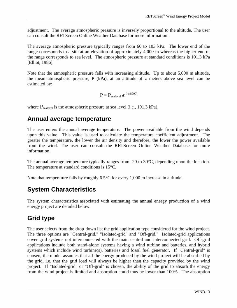
adjustment. The average atmospheric pressure is inversely proportional to the altitude. The user can consult the RETScreen Online Weather Database for more information. The average atmospheric pressure typically ranges from 60 to 103 kPa. The lower end of the range corresponds to a site at an elevation of approximately 4,000 m whereas the higher end of the range corresponds to sea level. The atmospheric pressure at standard conditions is 101.3 kPa [Elliot, 1986]. Note that the atmospheric pressure falls with increasing altitude. Up to about 5,000 m altitude, the mean atmospheric pressure, P (kPa), at an altitude of z meters above sea level can be estimated by:
P = Psealevel e (-z/8200)
where Psealevel is the atmospheric pressure at sea level (i.e., 101.3 kPa). Annual average temperature The user enters the annual average temperature. The power available from the wind depends upon this value. This value is used to calculate the temperature coefficient adjustment. The greater the temperature, the lower the air density and therefore, the lower the power available from the wind. The user can consult the RETScreen Online Weather Database for more information. The annual average temperature typically ranges from -20 to 30°C, depending upon the location. The temperature at standard conditions is 15°C. Note that temperature falls by roughly 6.5°C for every 1,000 m increase in altitude. System Characteristics The system characteristics associated with estimating the annual energy production of a wind energy project are detailed below. Grid type The user selects from the drop-down list the grid application type considered for the wind project. The three options are "Central-grid," "Isolated-grid" and "Off-grid." Isolated-grid applications cover grid systems not interconnected with the main central and interconnected grid. Off-grid applications include both stand-alone systems having a wind turbine and batteries, and hybrid systems which include wind turbine(s), batteries and fossil fuel generator. If "Central-grid" is chosen, the model assumes that all the energy produced by the wind project will be absorbed by the grid, i.e. that the grid load will always be higher than the capacity provided by the wind project. If "Isolated-grid" or "Off-grid" is chosen, the ability of the grid to absorb the energy from the wind project is limited and absorption could thus be lower than 100%. The absorption
WIND.13
RETScreen® Software Online User Manual
rate will depend on the penetration level of the wind project with respect to the peak load of the grid and wind speed at the site. Peak load The user enters the peak electrical load (kW) of the electric utility. For isolated-grid cases, this is the maximum electric power demand that the utility faces during the year, and for off-grid cases, this is the maximum electric power demand of the application during the year. The peak load is used to calculate the penetration level of the wind farm on the grid. Wind turbine rated power The user enters the wind turbine rated power, also called rated capacity, in the Equipment Data worksheet and it is copied automatically to the Energy Model worksheet. The rated power is a performance characteristic of a particular wind turbine and is provided by the manufacturer of the equipment. This "capacity" is reached at the rated wind speed. The model uses the wind turbine rated power in combination with the number of turbines to calculate the wind plant capacity. For isolated areas, only small and medium size turbines are normally considered as the infrastructure required for the transportation and erection of the larger machines are usually not available in these areas [Brothers, 1993]. Note: At this point the user should complete the Equipment Data worksheet to specify the wind equipment for the project. Number of turbines The user enters the number of wind turbines desired. This item is used to calculate the total unadjusted energy production and the wind plant capacity. A large number of smaller turbines has the advantage of reducing the fluctuations in the total wind energy project output. On the other hand, the cost of large machines may be lower on a per kW basis. The user can perform a sensitivity analysis specifying different sizes of turbines to see the impact on the financial feasibility of the project. Wind plant capacity The model calculates the wind plant capacity, or power output of the wind turbines at the site in kW, as defined by the number and rated capacity of the wind turbines. Units switch: The user can choose to express the capacity in different units by selecting among the proposed set of units: "MW," "million Btu/h," "boiler hp," "ton (cooling)," "hp," "W." This value is for reference purposes only and is not required to run the model.
WIND.14
RETScreen® Wind Energy Project Model
Wind speed at... The model calculates the wind speed at the height entered by the user in the cell "Height of wind power density." Hub height The user enters the hub height in the Equipment Data worksheet and it is copied automatically to the Energy Model worksheet. The hub height is the height at which the centre of the rotor of a horizontal axis wind turbine is mounted. The hub height is used in the model to calculate the average wind speed at hub height. Whenever possible, increasing the hub height should be considered to improve the project's energy output. Note that only metric units are shown as these are the units utilised by the international wind energy industry. Wind speed at hub height The model calculates the wind speed at the hub height. This is the average speed of the wind that is powering the turbine rotor. It is calculated from the wind speed at 10 m, the hub height and the wind shear exponent. It is used to determine the unadjusted energy production from the wind equipment energy production curve. The wind speed at the hub height is usually significantly higher than the wind speed at 10 m due to wind shear. Generally, manufacturers do not supply turbine output data for wind speeds outside the range of 3 to 12 m/s. Thus, the model functions only for "Wind speeds at hub height" within the wind speeds range for which energy output data is calculated or pasted in the Equipment Data worksheet. Wind power density at hub height The model calculates the wind power density (W/m²) at the hub height. It is calculated for an air density of 1.225 kg/m³, corresponding to standard sea level pressure and a temperature of 15°C. Wind penetration level For "Isolated-grid" and "Off-grid" grid types, the model calculates the wind penetration level (%), which is the ratio of the "Wind plant capacity" over the "Peak load" of the local electric utility. The wind penetration level indicates the percentage of the peak electrical load that can be met by the wind equipment under rated wind speed conditions. Increasing the wind penetration level may improve the project's financial viability although sophisticated control systems might be needed at higher penetration levels. Although the wind penetration level can theoretically range from 0% to infinity, a range of 10 to 25% is more likely for isolated-grids. Penetration levels lower than 25% will not drastically affect the operation of an existing electrical generation system. Higher levels of penetration involve the use of sophisticated control systems and strategies, which can increase the project costs, but still may improve the overall financial viability of the project. For example, in a "high-penetration" wind-diesel hybrid system configuration, 100 to 200% penetration levels might be financially attractive. However, the model will be most accurate for levels lower than 25% and
WIND.15
RETScreen® Software Online User Manual
this should be sufficient for a preliminary feasibility analysis. For higher penetration levels, the user will have to provide the model with an estimate of the portion of the wind energy produced that can be absorbed by the isolated-grid or the off-grid system. Currently, most wind energy projects being implemented, even on isolated diesel-grids, have penetration levels of less than 25%. For very small off-grid systems, energy storage in batteries will likely be required. The RETScreen Wind Energy Project Model does not currently cover battery storage systems, although the blank worksheets can be used for this purpose. Suggested wind energy absorption rate For "Isolated-grid" and "Off-grid" grid types, the model calculates a suggested wind energy absorption rate (%). It is calculated using the wind speed at hub height and the wind penetration level. This value is not directly used for calculations in the model, it is only a suggested value that the user can use for the "Wind energy absorption rate" entered below. The model only provides suggested values for wind penetration levels less than 25%. However, if the wind penetration level is greater than 3% and the wind speed at hub height is 8.3 m/s and above, then the model does not provide suggested values. Under these circumstances, the wind energy absorption rates will vary widely depending on the configuration of the system and on the control strategies adopted. At the design stage, it is recommended to conduct a project specific simulation using an hourly model in order to derive a reasonable estimate for a suggested wind energy absorption rate. The "Suggested wind energy absorption rate" is likely conservative and is based upon typical load duration curves for isolated-grids. Other sources of information show higher absorption rates, all other things being equal. In the event that a sensitivity analysis indicates that the value of the wind energy absorption rate is critical to the financial feasibility of a project, it is best to run a time series model to determine its value more accurately. This is usually done as part of project design. Wind energy absorption rate For "Isolated-grid" and "Off-grid" grid types, the user enters the wind energy absorption rate, which is the percentage of the wind energy collected that can be absorbed by the isolated-grid or the off-grid system. It depends primarily on the wind penetration level and the average wind speed. Hence, under certain circumstances, such as high wind penetration level, high wind speed and low system load, there can be more wind energy collected than the electrical grid (actually "load") needs and only a portion will be accepted (or delivered) to the grid. The user can enter the "Suggested wind energy absorption rate" as the "Wind energy absorption rate." The wind energy absorption rate is used to calculate the wind energy delivered. For isolated-grid and off-grid applications in remote areas, values for the wind energy absorption rate will likely range from 60 to 100%. For penetration levels greater than 25%, the wind energy absorption rate depends to a greater extent on the control strategy adopted and the use of a time series model is suggested to be used during the design or engineering phase of the project development for a better estimate of the absorption rate. The lower end of the proposed range
WIND.16
RETScreen® Wind Energy Project Model
corresponds to a system for which the wind energy installed capacity is a large portion of the total electric utility load. The higher end of the range is representative of an electric utility system for which the wind energy installed capacity is a not significant portion of the total electric utility load [Rangi, 1992].
Array losses The user enters the estimated array losses (%). These are caused by the interaction of the wind turbines with each other through their wakes. Turbines in the "shadow" of others do not "see" as much wind as the front ones and energy production is decreased as a result. Array losses depend on the turbine spacing, orientation, site characteristics and topography. Array losses are used as an input in the model to calculate the losses coefficient. Typical values for a well designed wind farm range from 0 to 20% of "Gross energy production." The lower end of the range corresponds to small clusters of well spaced turbines while the higher end of the range corresponds to a closely packed wind farm with a weak dominant wind. Array losses for a single turbine installation are 0% while a well designed cluster of less than 8 to 10 turbines should keep array losses below 5% [Conover, 1994]. Note: The user has to be careful not to overstate these potential losses and the losses in the following cells. Airfoil soiling and/or icing losses The user enters airfoil soiling and/or icing losses (%). Airfoil soiling losses are caused by soiling of the blades from such things as bugs and/or ice build-up. Accumulation of bugs or ice affects the aerodynamic performance of the blades. It can be improved by washing the blades regularly or heating the edge of the blades. Icing losses occur when accumulation of ice forces a wind machine to shut down or prevents it from starting. Icing losses depend on the ambient temperature, the altitude at which the machine is installed, the level of humidity and the machine design. Airfoil soiling and icing losses are used as an input in the model to calculate the losses coefficient. Typical values range from 1 to 10% of "Gross energy production" [Conover, 1994] [WECTEC, 1996]. Other downtime losses The user enters other downtime losses (%). These are the result of scheduled maintenance, wind turbine failures, station outage and utility outage. Other downtime losses are used as an input in the model to calculate the losses coefficient. Typical values range from 2 to 7% of "Gross energy production." In the case of wind turbines installed in extreme environments (arctic climate, weak grid, etc.), losses are more likely to be toward the higher end of the range [Conover, 1994]. Miscellaneous losses The user enters miscellaneous losses (%), which represents losses of energy production due to starts and stops, off-yaw operation, high wind and cut-outs from wind gusts. They also include
WIND.17
RETScreen® Software Online User Manual
any parasitic power requirements and any transmission line losses from the wind energy project site to the point where the project connects to the local distribution grid. Miscellaneous losses are used as an input in the model to calculate the losses coefficient. Typical values range from 2 to 6% of "Gross energy production" [Conover, 1994]. Annual Energy Production Items associated with calculating the annual energy production of a wind energy project are detailed below. Wind plant capacity The model calculates the wind plant capacity, or power output of the wind turbines at the site in kW, as defined by the number and rated capacity of the wind turbines. Units switch: The user can choose to express the capacity in different units by selecting among the proposed set of units: "MW," "million Btu/h," "boiler hp," "ton (cooling)," "hp," "W." This value is for reference purposes only and is not required to run the model. Unadjusted energy production The model calculates the unadjusted energy production from the wind equipment, in MWh. It is the energy that one or more wind turbines will produce at standard conditions of temperature and atmospheric pressure. The calculation is based on the energy production curve of the selected wind turbine (entered in the Equipment Data worksheet) and on the average wind speed at hub height for the proposed site. Pressure adjustment coefficient The model calculates the pressure adjustment coefficient, which is proportional to the average atmospheric pressure at the site, which in turn depends primarily on site elevation. It is used to determine the gross energy production. The coefficient should fall between 0.59 and 1.02 with the lower end of the range corresponding to a site at an altitude of more than 4,000 m. Temperature adjustment coefficient The model calculates the temperature adjustment coefficient, which is inversely proportional to the average temperature at the site. It is used to determine the gross energy production. The standard rating temperature of 15°C for wind turbine performance corresponds to a temperature adjustment coefficient of 1. Typically, the coefficient falls between 0.98 and 1.15 for temperature ranging approximately from 20°C to -20°C. Gross energy production The model calculates the gross energy production (MWh), which is the total annual energy produced by the wind energy equipment, before any losses, at the wind speed, atmospheric
WIND.18
RETScreen® Wind Energy Project Model
pressure and temperature conditions at the site. It is derived from the unadjusted energy production, the pressure adjustment coefficient and the temperature adjustment coefficient. It is used to determine the renewable energy delivered. Losses coefficient The model calculates the losses coefficient, which integrates all the loss factors. The coefficient is a combination of the array, airfoil soiling/icing, other downtime, and miscellaneous losses. It is used to calculate the renewable energy delivered. Losses coefficient of 0.75 or lower would be indicative of a poorly planned project. Specific yield The model calculates the specific yield (kWh/m²) of the wind energy equipment, which is a common criteria in the wind energy industry to evaluate and compare the performance of a wind turbine in conjunction with the wind regime at the site. The specific yield is obtained by dividing the renewable energy delivered by a wind turbine by the swept area of the rotor. The specific yield normally ranges from 150 to 1,500 kWh/m² per turbine where the low end corresponds to a small wind turbine in a mediocre wind regime and the high end, to a larger wind turbine in a good wind regime. Wind plant capacity factor The model calculates the wind plant capacity factor (%), which represents the ratio of the average power produced by the plant over a year to its rated power capacity. It is calculated as the ratio of the renewable energy delivered (or renewable energy collected in the case of isolated-grid or off-grid system) over the wind plant capacity multiplied by the total hours in a year. The wind plant capacity factor will typically range from 20 to 40%. The lower end of the range is representative of older technologies installed in average wind regimes while the higher end of the range represents the latest wind turbines installed in good wind regimes. Renewable energy collected For "Isolated-grid" and "Off-grid" grid types, the model calculates the renewable energy collected (MWh), which is the net amount of energy produced by the wind energy equipment. The model uses the gross energy production and the losses coefficient to calculate this value. Renewable energy delivered The model calculates the annual renewable energy delivered (MWh) to the grid, which is the amount of wind energy that is transformed into electricity and therefore replaces the energy that would have otherwise been produced by the existing utility system using the base case electricity system. For isolated-grid and off-grid applications, the renewable energy delivered is derived from the renewable energy collected and the wind energy absorption rate. This value is transferred to the Financial Summary worksheet as an input to conduct the financial analysis.
WIND.19
RETScreen® Software Online User Manual
Units switch: The user can choose to express the energy in different units by selecting among the proposed set of units: "GWh," "Gcal," "million Btu," "GJ," "therm," "kWh," "hp-h," "MJ." This value is for reference purposes only and is not required to run the model. Excess RE (Renewable Energy) available For "Isolated-grid" and "Off-grid" grid types, the model calculates the excess renewable energy available (MWh), which is the portion of the renewable energy collected that cannot be absorbed by the isolated-grid (load) or off-grid application, and therefore is available for heating or other purposes. It is calculated as the difference between the renewable energy collected and the renewable energy delivered. This value is transferred to the Financial Summary worksheet as an input to conduct the financial analysis.
WIND.20
RETScreen® Wind Energy Project Model
Equipment Data As part of the RETScreen Clean Energy Project Analysis Software, the Equipment Data worksheet is used to specify the wind equipment for the project. The results of this worksheet are transferred to the Energy Model worksheet. The user should return to the Energy Model worksheet after completing the Equipment Data worksheet. Wind Turbine Characteristics The wind turbine characteristics are detailed below. Wind turbine rated power The user enters the wind turbine rated power (kW). The rated power is a performance characteristic of a particular wind turbine and is provided by the manufacturer of the equipment. This capacity is reached at the rated wind speed. The user can consult the RETScreen Online Product Database for more information. Hub height The user enters the hub height (m). The hub height is the height at which the centre of the rotor of an horizontal axis wind turbine is mounted. Whenever possible, increasing the hub height should be considered to improve the project's energy output. Typical hub heights of turbines range from 6 to 100 m. Tower heights have increased during the past few years as the technology is becoming more mature. The user can consult the RETScreen Online Product Database for more information. Note that only metric units are shown as these are the units utilised by the international wind energy industry. Rotor diameter The user enters the rotor diameter (m), which is the diameter of the circle formed by the rotation of the blades. This information is given for reference purposes only. The rotor diameter of the turbines commercially available typically range from 7 to 80 m or more. The user can consult the RETScreen Online Product Database for more information. Swept area The user enters the swept area (m²), which is the area perpendicular to the wind direction that a rotor will cover during one complete rotation. The power and energy output of a wind turbine is strongly related to the swept area of its rotor. The swept area of turbines can range from 35 to 5,027 m² or more. The user can consult the RETScreen Online Product Database for more information.
WIND.21
RETScreen® Software Online User Manual
Wind turbine manufacturer The user enters the name of the wind turbine manufacturer. This information is given for reference purposes only. The user can consult the RETScreen Online Product Database for more information. Wind turbine model The user enters the name of the wind turbine model. This information is given for reference purposes only. The user can consult the RETScreen Online Product Database for more information. Energy curve data source The user selects the energy curve data source to determine how the energy curve data will be calculated for the wind turbine specified. The options from the drop-down list are: "Standard," "Custom" and "User-defined." Changing the selection in this field affects the worksheet display and calculation for the energy curve data. The energy curve data is calculated using the wind turbine power curve data and the wind speed distribution. When the option "Standard" is selected, the model will calculate the energy curve data based on a Rayleigh wind speed distribution. For a first approximation, the user can use the standard option if the wind speed distribution at the site is not known. Note that the Rayleigh distribution is a special case of the Weibull distribution for which the shape factor equals 2. When the option "Custom" is selected, the model will calculate the energy curve data based on a Weibull wind speed distribution. This distribution is often used in wind energy engineering, as it conforms well to the observed long-term distribution of mean wind speeds for a range of sites. In this case, the user specifies the shape factor that will be used in the calculations. Selecting the "User-defined" option allows the user to enter the energy curve data directly or to paste values from the RETScreen Online Product Database. In this case, the power curve data is given for reference purposes only and it is not required to run the model. If "Wind power density" is selected as the wind data source in the Energy Model worksheet, then the "User-defined" option is not available for the "Energy curve data source" cell.
Shape factor The user enters a value for the shape factor which is a characteristic of the Weibull distribution. Typically the shape factor will range from 1 to 3. For a given average wind speed, a lower shape factor indicates a relatively wide distribution of wind speeds around the average while a higher shape factor indicates a relatively narrow distribution of wind speeds around the average. A lower shape factor is indicative of a higher wind energy density for a given average wind speed. This will normally lead to a higher energy production, except for sites with a high average wind
WIND.22
RETScreen® Wind Energy Project Model
speed, in which case energy production will be curtailed due to the greater occurrence of wind speeds higher than turbine cut-out wind speed. Wind Turbine Production Data In this section, the wind turbine production data are calculated by the model or entered by the user. Wind speed This is a range of possible wind speeds, in m/s, for which power curve data and energy curve data are entered. When used in conjunction with the power curve data, the wind speeds indicated correspond to instantaneous wind speeds. When used in conjunction with the energy curve data, the wind speeds indicated correspond to the annual average value of the wind speed distribution. Power curve data The user enters the wind turbine power curve data (kW) which is the instantaneous energy (i.e. power) delivered by the wind turbine measured over its operating range of wind speeds at hub height. This performance characteristic is usually provided by the wind turbine manufacturer. The model assumes that the power output is rated at 15 °C and 101.3 kPa. The user can consult the RETScreen Online Product Database for more information. If "Standard" or "Custom" option is selected in the "Energy curve data source" input cell, the model assumes that the wind turbine selected has a cut-out wind speed of 25 m/s i.e. the turbine is shut off for all wind speeds greater than 25 m/s. If the "User-defined" option in the "Energy curve data source" input cell is chosen, the power curve data is entered for reference purposes only and is not required to run the model. Energy curve data The energy curve data (MWh/yr) is the total amount of energy a wind turbine produces over a range of annual average wind speeds. The model calculates this value if the user has selected the "Standard" or "Custom" option for the "Energy curve data source." However, if the "User-defined" option for the "Energy curve data source" is selected, the user enters the energy curve data over the range of possible annual average wind speeds. The user can consult the RETScreen Online Product Database for more information. Note: The user should return to the Energy Model worksheet.
WIND.23

RETScreen® Software Online User Manual
Wind Turbine Power and Energy Curves This graph provides a representation of the power (in kW) and energy (in MWh/yr) delivered by the wind turbine measured over a range of wind speeds. The graph is based on values from the power curve data and energy curve data columns above. Note: The user should return to the Energy Model worksheet.
WIND.24
RETScreen® Wind Energy Project Model
Cost Analysis1
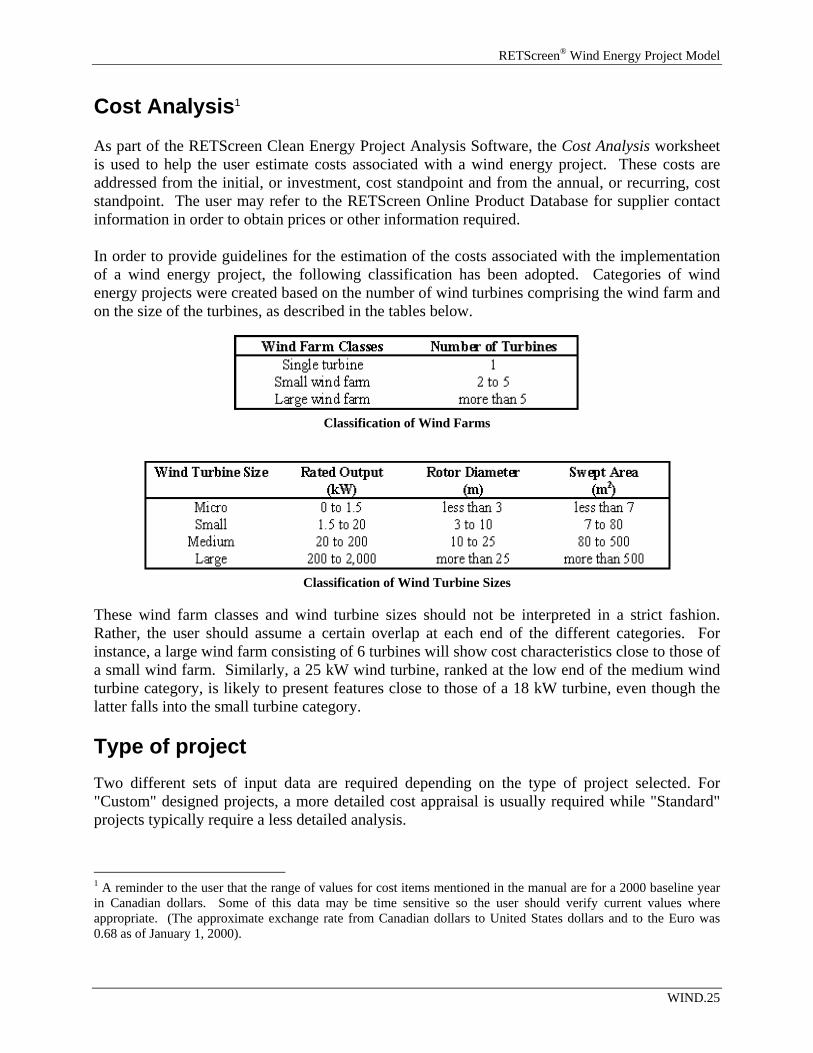
As part of the RETScreen Clean Energy Project Analysis Software, the Cost Analysis worksheet is used to help the user estimate costs associated with a wind energy project. These costs are addressed from the initial, or investment, cost standpoint and from the annual, or recurring, cost standpoint. The user may refer to the RETScreen Online Product Database for supplier contact information in order to obtain prices or other information required. In order to provide guidelines for the estimation of the costs associated with the implementation of a wind energy project, the following classification has been adopted. Categories of wind energy projects were created based on the number of wind turbines comprising the wind farm and on the size of the turbines, as described in the tables below.
Classification of Wind Farms
Classification of Wind Turbine Sizes
These wind farm classes and wind turbine sizes should not be interpreted in a strict fashion. Rather, the user should assume a certain overlap at each end of the different categories. For instance, a large wind farm consisting of 6 turbines will show cost characteristics close to those of a small wind farm. Similarly, a 25 kW wind turbine, ranked at the low end of the medium wind turbine category, is likely to present features close to those of a 18 kW turbine, even though the latter falls into the small turbine category. Type of project Two different sets of input data are required depending on the type of project selected. For "Custom" designed projects, a more detailed cost appraisal is usually required while "Standard" projects typically require a less detailed analysis.
1 A reminder to the user that the range of values for cost items mentioned in the manual are for a 2000 baseline year in Canadian dollars. Some of this data may be time sensitive so the user should verify current values where appropriate. (The approximate exchange rate from Canadian dollars to United States dollars and to the Euro was 0.68 as of January 1, 2000).
WIND.25
RETScreen® Software Online User Manual
Currency To perform a RETScreen project analysis, the user may select a currency of their choice from the "Currency" cell in the Cost Analysis worksheet. The user selects the currency in which the monetary data of the project will be reported. For example, if the user selects "$," all monetary related items are expressed in $. Selecting "User-defined" allows the user to specify the currency manually by entering a name or symbol in the additional input cell that appears adjacent to the currency switch cell. The currency may be expressed using a maximum of three characters ($US, £, ¥, etc.). To facilitate the presentation of monetary data, this selection may also be used to reduce the monetary data by a factor (e.g. $ reduced by a factor of a thousand, hence k$ 1,000 instead of $ 1,000,000). If "None" is selected, all monetary data are expressed without units. Hence, where monetary data is used together with other units (e.g. $/kWh) the currency code is replaced with a hyphen (-/kWh). The user may also select a country to obtain the International Standard Organisation (ISO) three-letter country currency code. For example, if Afghanistan is selected from the currency switch drop-down list, all project monetary data are expressed in AFA. The first two letters of the country currency code refer to the name of the country (AF for Afghanistan), and the third letter to the name of the currency (A for Afghani). For information purposes, the user may want to assign a portion of a project cost item in a second currency, to account for those costs that must be paid for in a currency other than the currency in which the project costs are reported. To assign a cost item in a second currency, the user must select the option "Second currency" from the "Cost references" drop-down list cell. Some currency symbols may be unclear on the screen (e.g. €); this is caused by the zoom settings of the sheet. The user can then increase the zoom to see those symbols correctly. Usually, symbols will be fully visible on printing even if not fully appearing on the screen display. Cost references The user selects the reference (from the Cost Analysis worksheet) that will be used as a guideline for the estimation of costs associated with the implementation of the project. This feature allows the user to change the "Quantity Range" and the "Unit Cost Range" columns. The options from the drop down list are: "Canada - 2000," "None," "Second currency" and a selection of 8 user-defined options ("Enter new 1," "Enter new 2," etc.). If the user selects "Canada - 2000" the range of values reported in the "Quantity Range" and "Unit Cost Range" columns are for a 2000 baseline year, for projects in Canada and in Canadian dollars. This is the default selection used in the built-in example in the original RETScreen file.
WIND.26
RETScreen® Wind Energy Project Model
Selecting "None" hides the information presented in the "Quantity Range" and "Unit Cost Range" columns. The user may choose this option, for example, to minimise the amount of information printed in the final report. If the user selects "Second currency" two additional input cells appear in the next row: "Second currency" and "Rate: 1st currency / 2nd currency." In addition, the "Quantity Range" and "Unit Cost Range" columns change to "% Foreign" and "Foreign Amount," respectively. This option allows the user to assign a portion of a project cost item in a second currency, to account for those costs that must be paid for in a currency other than the currency in which the project costs are reported. Note that this selection is for reference purposes only, and does not affect the calculations made in other worksheets. If "Enter new 1" (or any of the other 8 selections) is selected, the user may manually enter quantity and cost information that is specific to the region in which the project is located and/or for a different cost base year. This selection thus allows the user to customise the information in the "Quantity Range" and "Unit Cost Range" columns. The user can also overwrite "Enter new 1" to enter a specific name (e.g. Japan - 2001) for a new set of unit cost and quantity ranges. The user may also evaluate a single project using different quantity and cost ranges; selecting a new range reference ("Enter new 1" to "Enter new 8") enables the user to keep track of different cost scenarios. Hence the user may retain a record of up to 8 different quantity and cost ranges that can be used in future RETScreen analyses and thus create a localised cost database. Second currency The user selects the second currency; this is the currency in which a portion of a project cost item will be paid for in the second currency specified by the user. The second currency option is activated by selecting "Second currency" in the "Cost references" drop-down list cell. This second unit of currency is displayed in the "Foreign Amount" column. If the user selects "$," the unit of currency shown in the "Foreign Amount" column is "$". Selecting "User-defined" allows the user to specify the currency manually by entering a name or symbol in the additional input cell that appears adjacent to the currency switch cell. The currency may be expressed using a maximum of three characters ($US, £, ¥, etc.). To facilitate the presentation of monetary data, this selection may also be used to reduce the monetary data by a factor (e.g. $ reduced by a factor of a thousand, hence k$ 1,000 instead of $ 1,000,000). If "None" is selected, no unit of currency is shown in the "Foreign Amount" column. The user may also select a country to obtain the International Standard Organisation (ISO) three-letter country currency code. For example, if Afghanistan is selected from the currency switch drop-down list, the unit of currency shown in the "Foreign Amount" column is "AFA." The first two letters of the country currency code refer to the name of the country (AF for Afghanistan), and the third letter to the name of the currency (A for Afghani).
WIND.27

RETScreen® Software Online User Manual
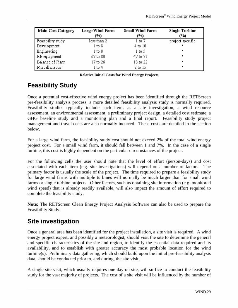
Some currency symbols may be unclear on the screen (e.g. €); this is caused by the zoom settings of the sheet. The user can then increase the zoom to see those symbols correctly. Usually, symbols will be fully visible on printing even if not fully appearing on the screen display. Rate: 1st currency / 2nd currency The user enters the exchange rate between the currency selected in "Currency" and the currency selected in "Second currency." The exchange rate is used to calculate the values in the "Foreign Amount" column. Note that this selection is for reference purposes only, and does not affect the calculations made in other worksheets. For example, the user selects the Afghanistan currency (AFA) as the currency in which the monetary data of the project is reported (i.e. selection made in "Currency" input cell) - this is the 1st currency. The user then selects United States currency (USD) from the "Second currency" input cell - this is the 2nd currency. The user then enters the exchange rate in the "Rate: AFA/USD" input cell i.e. the amount of AFA needed to purchase 1 USD. Using this feature the user can then specify what portion (in the "% Foreign" column) of a project cost item's costs will be paid for in USD. % Foreign The user enters the percentage of an item's costs that will be paid for in the second currency. The second currency is selected by the user in the “Second currency” cell. Foreign Amount The model calculates the amount of an item's costs that will be paid for in the second currency. This value is based on the exchange rate and the percentage of an items costs that will be paid for in the second currency, as specified by the user. Initial Costs (Credits) The initial costs associated with the implementation of the project are detailed on the next page. The major categories include costs for preparing a feasibility study, performing the project development functions, completing the necessary engineering, purchasing and installing the energy equipment, construction of the balance of plant and costs for any other miscellaneous items. The energy equipment and balance of plant are the two cost categories showing the strongest dependence on the number of wind turbines that make up the wind farm. Hence, the larger the wind farm, the more relative weight these two categories represent. The following table suggests typical ranges of relative costs, for the main cost categories, according to the wind farm class being analysed [Conover, 1994], [Zond, 1994] and [Vesterdal, 1992].
WIND.28
RETScreen® Wind Energy Project Model
Relative Initial Costs for Wind Energy Projects
Feasibility Study Once a potential cost-effective wind energy project has been identified through the RETScreen pre-feasibility analysis process, a more detailed feasibility analysis study is normally required. Feasibility studies typically include such items as a site investigation, a wind resource assessment, an environmental assessment, a preliminary project design, a detailed cost estimate, a GHG baseline study and a monitoring plan and a final report. Feasibility study project management and travel costs are also normally incurred. These costs are detailed in the section below. For a large wind farm, the feasibility study cost should not exceed 2% of the total wind energy project cost. For a small wind farm, it should fall between 1 and 7%. In the case of a single turbine, this cost is highly dependent on the particular circumstances of the project. For the following cells the user should note that the level of effort (person-days) and cost associated with each item (e.g. site investigations) will depend on a number of factors. The primary factor is usually the scale of the project. The time required to prepare a feasibility study for large wind farms with multiple turbines will normally be much larger than for small wind farms or single turbine projects. Other factors, such as obtaining site information (e.g. monitored wind speed) that is already readily available, will also impact the amount of effort required to complete the feasibility study. Note: The RETScreen Clean Energy Project Analysis Software can also be used to prepare the Feasibility Study. Site investigation Once a general area has been identified for the project installation, a site visit is required. A wind energy project expert, and possibly a meteorologist, should visit the site to determine the general and specific characteristics of the site and region, to identify the essential data required and its availability, and to establish with greater accuracy the most probable location for the wind turbine(s). Preliminary data gathering, which should build upon the initial pre-feasibility analysis data, should be conducted prior to, and during, the site visit. A single site visit, which usually requires one day on site, will suffice to conduct the feasibility study for the vast majority of projects. The cost of a site visit will be influenced by the number of
WIND.29
RETScreen® Software Online User Manual
persons considered necessary to participate in the visit, the planned duration and travel time (travel costs separate - see below) to and from the site. The time required to gather the data prior to the site visit and during the site visit typically falls between 2 and 8 person-days. The average per daily fees of the personnel making the visit(s) will range from $200 to $800, depending on their experience. Wind resource assessment Reliable wind resource data for the project site is critical for preparing a proper feasibility study. A wind resource assessment consists of the installation of one or more meteorological towers at the site, the collection and the analysis of the wind resource data. At least one year of measurement is recommended. Characteristics of the wind resource other that average annual wind speed, such as temperature, wind speed frequency distribution, turbulence intensity, icing occurrence, directional predominance, seasonal and diurnal variability, and distribution and duration of calm periods may also be of interest to the design and assessment of performance of a wind energy project. The cost of a one year wind resource assessment typically falls between $10,000 and $25,000 per meteorological tower (excluding travel expenses). The cost depends mainly on the tower height, the number and type of instruments mounted on the tower, on whether the required equipment is purchased or rented and on the scope of the analysis required. The number of towers varies according to the number of sites considered and the scale of the project. One or two towers will normally suffice for a single turbine or a small wind farm. On the other hand, a large wind farm sited in complex terrain may justify the use of a number of meteorological towers corresponding to half the number of turbines forming the wind farm. Environmental assessment An environmental assessment is an essential part of the feasibility study work. While wind energy projects can usually be developed in an environmentally acceptable manner (projects can often be designed to enhance environmental conditions), work is required to study the potential environmental impacts of any proposed wind energy project. At the feasibility study stage, the objective of the environmental assessment is to determine if there are any major environmental impact that could prevent the implementation of a project. Noise and visual impacts as well as potential impact on the flora and fauna must be addressed. The time required to consult with the different stakeholders, gather and process relevant data and possibly visit the site and local communities typically falls between 1 and 8 person-days. The average per daily fees of the personnel making the assessment will range from $200 to $800, depending on their experience. Preliminary design A preliminary design is required in order to determine the optimum plant capacity, the size and layout of the structures and equipment, and the estimated construction quantities necessary for the detailed cost estimate. As with site investigations, the scope of this task is often reduced for
WIND.30
RETScreen® Wind Energy Project Model
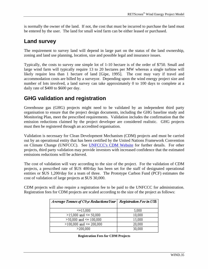
small projects in order to reduce costs. Consequently, additional contingencies should be allowed to account for the resulting additional risk of cost overruns during construction. The cost of the preliminary design is calculated based on an estimate of the time required by an expert to complete the necessary work. The cost of professional services required to complete a preliminary design will range between $200 and $800 per person-day. As with site investigations, the time required to complete the preliminary design will depend, to a large extend on the size of the project and corresponding acceptable level of risk. The number of person-days required can range between 2 and 20. Detailed cost estimate The detailed cost estimate for the proposed wind energy project is based on the results of the preliminary design and other investigations carried out during the feasibility study. The cost of preparing the detailed cost estimate is calculated based on an estimate of the time required by an expert to complete the necessary work. Engineering services for completing a wind energy project detailed cost estimate will range between $200 and $800 per person-day. The number of person-days required to complete the cost estimate will range between 3 and 20 depending on the size of the project and acceptable level of risk. GHG baseline study and monitoring plan In order for the greenhouse gas (GHG) emissions reductions generated from a project to be recognised and sold on domestic or international carbon markets, several project documents need to be developed, the key elements of which are a GHG baseline study and a Monitoring Plan (MP). A GHG baseline study identifies and justifies a credible project baseline based on the review of relevant information such as grid expansion plans, dispatch models, fuel use on the margin, current fuel consumption patterns and emissions factors. The GHG baseline study sets a project boundary and identifies all sources of GHG emissions that would have occurred under the baseline scenario, i.e. the scenario most likely to have occurred if the project were not implemented. A Monitoring Plan identifies the data that needs to be collected in order to monitor and verify the emissions reductions resulting from the project and describes a methodology for quantifying these reductions as measured against the project baseline. An outside consultant or team is often called in to develop the baseline study and monitoring plan. However, as more project examples become available and standardised methodologies are accepted, these studies may be more easily carried out by project proponents. Costs will depend on the complexity of the baseline, the size of the project and the availability of sectoral or regional baselines and standardised monitoring methodologies. Costs for developing baseline studies and monitoring plans for large projects have ranged from $US 30,000- $US 40,000 according to analysis by the Prototype Carbon Fund (PCF). Requirements for Clean Development Mechanism (CDM) projects are generally more stringent than for Joint Implementation (JI) or other projects. For example, CDM projects must also be monitored for their contribution to sustainable development of the host country. The rules governing baselines and monitoring for CDM can be found at UNFCCC's CDM Website. Note that for small-scale projects (renewable energy electricity projects with a capacity of 15 MW or
WIND.31
RETScreen® Software Online User Manual
less), it might not be necessary to carry out a full baseline study as simplified baselines and monitoring methodologies are available. Note: The optional GHG Analysis worksheet in RETScreen can be used to help prepare the baseline study. Report preparation A summary report should be prepared. It will describe the feasibility study, its findings and recommendations. The written report will contain data summaries, charts, tables and illustrations which clearly describe the proposed project. This report should be in sufficient detail regarding costs, performance and risks to enable project investors and other decision makers to evaluate the merits of the project. The cost of the report preparation is calculated based on an estimate of the time required by an expert to complete the necessary work. Preparing a feasibility study report will involve between 2 and 15 person-days at a rate of between $200 and $800 per person-day. Project management The project management cost item should cover the estimated costs of managing all phases of the feasibility study for the project, including the time required for stakeholder consultations. Consultations with the stakeholders in a given project are called for in order to build support and collaboration toward the project, and to identify any opposition at the earliest stage of development. The cost of the management of the feasibility study is calculated based on an estimate of the time required by an expert to complete the necessary work. It will involve between 2 and 8 person-days at a rate of between $300 and $800 per person-day. In addition, the time required to present the project to the stakeholders should not exceed an additional 3 person-days (travel time must also be added). Travel and accommodation This cost item includes all travel related costs (excluding time) required to prepare all sections of the feasibility study by the various members of the feasibility study team. These expenses include such things as airfare, car rental, lodging and per diem rates for each trip required. In the case of isolated areas, rates for air travel will vary markedly. Airfares are typically twice those for similar distances in populated areas. Since travel is a large component of the cost of doing work in isolated areas and the range of cost so variable, it is advised to contact a travel agent with experience in arranging such travel. Accommodation rates are typically twice the going rate for modest accommodation in populated areas. Typical rates for modest hotel rooms can range from $180 to $250 per day in the more isolated areas.
WIND.32
RETScreen® Wind Energy Project Model
Other These input cells are provided to allow the user to enter cost or credit items that are not included in the information provided in the above cost category. The user must enter a positive numerical value in the "Unit Cost" column. A cost item may be entered in the grey input cell as "Other." The user then selects "Cost" from the drop-down list in the unit column. The user can input both a quantity amount and unit cost. This item is provided to allow for project, technology and/or regional differences not specifically covered in the generic information provided. A credit item may be entered in the grey input cell as "Credit." The user then selects "Credit" from the drop-down list in the unit column. The project may be credited for material and/or labour costs that would have been spent on the base case, or conventional, energy system. The user can input both a quantity amount and unit cost. Note that the credit item is expressed as a negative value in the "Amount" column.
Development Once a potential wind energy project has been identified through the feasibility study to be desirable to implement, project development activities follow. For some projects, the feasibility study, development and engineering activities may proceed in parallel, depending on the risk and return acceptable to the project proponent. For wind energy projects, there are a number of possible project developers. Currently, a common approach is for private power developers to develop and own wind farms, where the energy is sold to the local electric utility or major local electric customers. In other cases the electric utility may develop and own wind farms directly. There are also a number of situations where individual wind turbines are purchased by individual investors or businesses and the energy is then sold back to the utility. Wind energy project development activities typically include costs for such items as power purchase agreement negotiations, permits and approvals, land rights, land surveys, GHG validation and registration, project financing, legal and accounting, project development management and travel costs. These costs are detailed in the section below. For a large wind farm, the development cost should fall between 1 and 8% of the total wind energy project cost. For a small wind farm, it should fall between 4 and 10%. In the case of a single turbine, this cost is highly dependent on the particular circumstances of the project. PPA negotiation The negotiation of a Power Purchase Agreement (PPA) is one of the first required steps of the project development stage for non-utility generators. A PPA negotiation will be required if the project is to be owned privately, rather than by a utility, and will also involve legal and other professional advice (e.g. finance, accounting). The scope of the work involved in the PPA
WIND.33

RETScreen® Software Online User Manual
negotiation will depend on whether or not conditions for the sale of power already exist (e.g. utility policy to purchase private power). The cost of the negotiation of the PPA is calculated based on an estimate of the time required by experts to complete the necessary work. The number of person-days required can range between 0 and 30 person-days or more depending on the complexity of the contract. The cost of professional services required for the negotiation of a PPA will range between $300 and $1,500 per person-day. Permits and approvals A number of permits and approvals may be required for the construction of the project. These include environmental approvals (e.g. federal, state/provincial), authorisations regarding the use of land (e.g. state/provincial, local), air traffic (e.g. federal), building permits (e.g. state/provincial, local), use of water resource (e.g. state/provincial), use of navigable waters (e.g. federal) and operating agreements (e.g. state/provincial, local). For a large wind farm, environmental approvals are likely to be the longest and most costly authorisations to obtain. The cost of acquiring the necessary permits and approvals is calculated based on an estimate of the time required by an expert to complete the necessary work. For wind energy projects it can involve between 0 and 400 person-days, depending on the scale, location and complexity of the project. Rates of between $200 and $800 per day are common. As an example, wind farm projects in the 50 to 100 MW scale range can require up to 400 person-days to obtain the required permits and approvals. Local laws for different scale projects can also have a significant impact on the amount of time required to receive the necessary approvals. In addition, the number of landowners that are involved in the project can also have a large impact on the time required to develop the project. On the other hand, small wind farm and/or single turbine projects may require only a minimal effort to obtain permits and approvals. Land rights Land rights are required for the land on which the wind energy project is located, including the service road, transmission and collection lines, substation and O&M building. Right-of-way may be granted for the access road and electric lines. The land required for the project infrastructure may be leased or purchased. The user enters the total estimated cost of purchasing the required land that cannot be leased or used under a right-of-way agreement. The cost should include an allowance for legal fees. Note that the estimated cost of negotiating any land lease and rights-of-way agreements should be included under the "Permits and approvals" section described above. For large wind farms, the land is usually leased. In this case, the cost of the land rights must appear as an annual payment in the annual cost section described below and therefore, the user enters 0 as the initial cost of land rights. In the case of a single turbine, the owner of the turbine
WIND.34
RETScreen® Wind Energy Project Model
is normally the owner of the land. If not, the cost that must be incurred to purchase the land must be entered by the user. The land for small wind farm can be either leased or purchased. Land survey The requirement to survey land will depend in large part on the status of the land ownership, zoning and land use planning, location, size and possible legal and insurance issues. Typically, the costs to survey one simple lot of 1-10 hectare is of the order of $750. Small and large wind farm will typically require 13 to 20 hectares per MW whereas a single turbine will likely require less than 1 hectare of land [Gipe, 1995]. The cost may vary if travel and accommodation costs are billed by a surveyor. Depending upon the wind energy project size and number of lots involved, a land survey can take approximately 0 to 100 days to complete at a daily rate of $400 to $600 per day. GHG validation and registration Greenhouse gas (GHG) projects might need to be validated by an independent third party organisation to ensure that the project design documents, including the GHG baseline study and Monitoring Plan, meet the prescribed requirements. Validation includes the confirmation that the emission reductions claimed by the project developer are considered realistic. GHG projects must then be registered through an accredited organisation. Validation is necessary for Clean Development Mechanism (CDM) projects and must be carried out by an operational entity that has been certified by the United Nations Framework Convention on Climate Change (UNFCCC). See UNFCCC's CDM Website for further details. For other projects, third party validation may provide investors with increased confidence that the estimated emissions reductions will be achieved. The cost of validation will vary according to the size of the project. For the validation of CDM projects, a prescribed rate of $US 400/day has been set for the staff of designated operational entities or $US 1,200/day for a team of three. The Prototype Carbon Fund (PCF) estimates the cost of validation of large projects at $US 30,000. CDM projects will also require a registration fee to be paid to the UNFCCC for administration. Registration fees for CDM projects are scaled according to the size of the project as follows:
Registration Fees for CDM Projects
WIND.35

RETScreen® Software Online User Manual
Project financing The time and effort required to arrange project financing can be significant, even for a small project. Wind energy projects are usually capital intensive, long-term investments. The cost of financing will be comprised of the effort required by experts to make the arrangements, identify investors and solicit funds. Typical rates for such work are set at a percentage of the financed amount and may include a fixed commencement fee. The cost of project financing is calculated based on an estimate of the services required to secure both debt and equity commitments. Acquiring the necessary project financing will involve between 3 and 100 person-days at a rate of between $500 and $1,500 per person-day depending on the complexity of the proposed financing structure. As a rule-of-thumb, the cost of acquiring the necessary project financing should be about 1.5% of the total project cost. Legal and accounting Legal and accounting support will be required at different points throughout the development stages of the project. This cost item allows the user to account for legal and accounting services not included as part of other development cost items such as for establishing a company to develop the project, to prepare monthly and annual financial statements, for project accounting, etc. The requirement for legal support will depend on the arrangements for financing, ownership, insurance, assumption of liability and complexity of contracts and agreements. The cost of legal and accounting support is calculated based on an estimate of the time required by experts to provide these services throughout the development of the project. Legal and accounting support will involve between 3 and 100 person-days at a rate of between $300 and $1,500 per person-day depending on the complexity and size of the project. Project management The project management cost item should cover the estimated expenses of managing all phases of the development of the project (excluding construction supervision). Public relations are also included as part of the project management cost item. Public relations can be an important element for successful project implementation. The elapsed time for the development of a wind energy project can be up to 4 years. The project management time (not including the time to manage the feasibility study) will involve between 0.2 and 4 person-years at a rate of between $130,000 and $180,000 per person-year, depending on the scale of the project. A reasonable estimate for project management is 10% of the cost of the total development activities. However, the investment in public relations will depend on the level of local support deemed necessary to achieve a successful implementation of the project. For a large wind farm involving many stakeholders, such as landowners, and requiring an extensive number of permits and approvals, additional public relations related project management costs of up to $150,000 per year is not unusual.
WIND.36

RETScreen® Wind Energy Project Model
Travel and accommodation A number of field visits and other trips will be required during the development phase (primarily for meetings). This cost item includes all travel related costs (excluding time) required to develop the project.
Other These input cells are provided to allow the user to enter cost or credit items that are not included in the information provided in the above cost category. The user must enter a positive numerical value in the "Unit Cost" column. A cost item may be entered in the grey input cell as "Other." The user then selects "Cost" from the drop-down list in the unit column. The user can input both a quantity amount and unit cost. This item is provided to allow for project, technology and/or regional differences not specifically covered in the generic information provided. A credit item may be entered in the grey input cell as "Credit." The user then selects "Credit" from the drop-down list in the unit column. The project may be credited for material and/or labour costs that would have been spent on the base case, or conventional, energy system. The user can input both a quantity amount and unit cost. Note that the credit item is expressed as a negative value in the "Amount" column. Engineering The engineering phase includes costs for the wind energy project wind turbine(s) micro-siting, mechanical, electrical and civil design, tenders and contracting, and construction supervision. These costs are detailed below. For a large wind farm, the engineering costs should fall between 1 and 8% of the total wind energy project cost. For a small wind farm, it should fall between 1 and 5%. In the case of a single turbine, this cost is highly dependent on the particular circumstances of the project. Wind turbine(s) micro-siting Upon a decision to construct the wind energy project at the completion of the feasibility study, individual wind turbine micro-siting might be required due to site specific variations in winds due to topography, terrain, obstructions, land cover, etc. For large-scale projects, the bulk of the cost resides in the time invested by the micro-siting team. It can include energy and civil engineers, meteorologists, computer simulation experts and draftsmen. The cost of micro-siting will also include costs for necessary maps and topographical data and may include additional surveying. Depending upon the accuracy and appropriateness of wind resource data, it may be necessary to include the cost for a wind resource modelling expert to prepare a site assessment report. The cost of modelling will be influenced by the availability of digitised topographical maps and historical and/or recent wind speed data for the site and region. The cost of micro-siting should
WIND.37

RETScreen® Software Online User Manual
be based on an estimate of the time required by experts to complete the necessary work. It can involve between 0 and 300 person-days at a rate of between $200 and $800 depending on the complexity, from a siting point of view, of the proposed project. As an example, large wind farms in the 50 to 100 MW scale range will be at the high end of this range while a small wind farm may require a much lower effort of approximately 3 to 10 person-days. Mechanical design The principal mechanical engineering tasks will be associated with design and planning of the assembly and erection of equipment. The cost of the mechanical engineering should be based on an estimate of the time required by experts to complete the necessary work. It can involve between 2 and 150 person-days at a rate of between $200 and $800. As an example, large wind farms in the 50 to 100 MW scale range will be at the high end of this range while a small wind farm may require a much lower effort of approximately 3 to 10 person-days. Electrical design The principal electrical engineering tasks will be associated with design and planning of construction of the control and electrical protection systems and the electrical interconnection with the existing electrical grid. For instance, the interconnection study will address all safety aspects related to the addition of a new production source on the grid, as well as analyse the impact with respect to the quality of the power delivered. The level of effort will be influenced by the availability of appropriate design information from the wind turbine supplier and interconnection requirements from the utility. The cost of the electrical engineering should be based on an estimate of the time required by experts to complete the necessary work. It can involve between 3 and 300 person-days at a rate of between $200 and $800, depending upon the scale and complexity of the project. As an example, large wind farms in the 50 to 100 MW scale range will be at the high end of this range while a small wind farm may require a much lower effort of approximately 3 to 10 person-days.
Civil design The principal civil engineering tasks will be associated with design and planning of construction of the foundations, access roads and other on ground systems. The level of effort will be influenced by the availability of approved design information from the suppliers and site specific information regarding access, soil conditions, surface drainage and other physical conditions.
WIND.38
RETScreen® Wind Energy Project Model
The cost of the civil engineering should be based on an estimate of the time required by experts to complete the necessary work. It can involve between 3 and 300 person-days at a rate of between $200 and $800, depending upon the scale and complexity of the project. As an example, large wind farms in the 50 to 100 MW scale range will be at the high end of this range while a small wind farm may require a much lower effort of approximately 3 to 20 person-days. Tenders and contracting Upon completion of the various engineering tasks, tender documents usually are prepared for the purpose of selecting contractors to undertake the work. Once tenders are released, the contracting process is required to both negotiate and establish contracts for the completion of the project. The cost of the tendering and contracting process should be based on an estimate of the time required by professionals to complete the necessary work. It can involve between 4 and 300 person-days, depending on the complexity of the project at a rate of between $200 and $800. As an example, large wind farms in the 50 to 100 MW scale range will be at the high end of this range while a small wind farm may require a much lower effort of approximately 6 to 20 person-days. Construction supervision The construction supervision cost item summarises the estimated costs associated with ensuring that the project is constructed as designed. Construction supervision is provided either by the consultant overseeing the project or by the equipment supplier, or the project manager. Construction supervision involves regular visits to the job site to inspect the installation. Construction supervision will involve between 0 to 2 person-years at a rate of between $130,000 and $180,000 per person-year depending on the duration of the project construction schedule. For example, the installation of a small single turbine should not require more than 0.02 person-year (≈ 7 days) of supervision. Travel time to the site for construction supervision is in addition to the range given. Travels costs should be included in the development section above. Other These input cells are provided to allow the user to enter cost or credit items that are not included in the information provided in the above cost category. The user must enter a positive numerical value in the "Unit Cost" column. A cost item may be entered in the grey input cell as "Other." The user then selects "Cost" from the drop-down list in the unit column. The user can input both a quantity amount and unit cost. This item is provided to allow for project, technology and/or regional differences not specifically covered in the generic information provided.
WIND.39
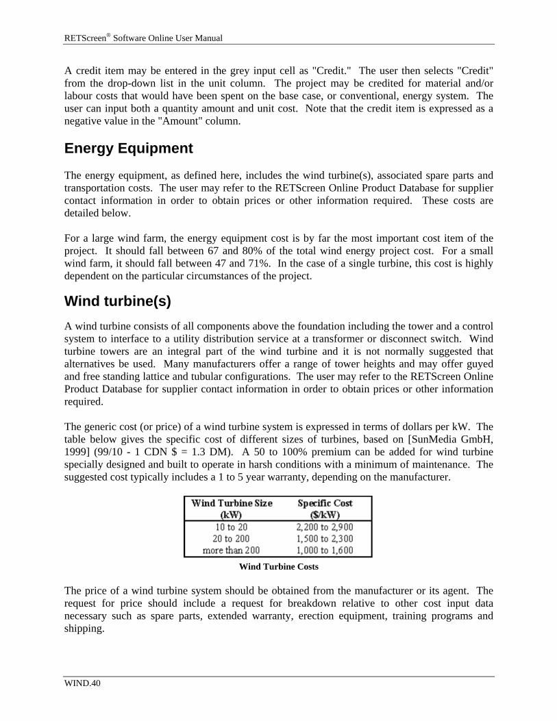
RETScreen® Software Online User Manual
A credit item may be entered in the grey input cell as "Credit." The user then selects "Credit" from the drop-down list in the unit column. The project may be credited for material and/or labour costs that would have been spent on the base case, or conventional, energy system. The user can input both a quantity amount and unit cost. Note that the credit item is expressed as a negative value in the "Amount" column. Energy Equipment The energy equipment, as defined here, includes the wind turbine(s), associated spare parts and transportation costs. The user may refer to the RETScreen Online Product Database for supplier contact information in order to obtain prices or other information required. These costs are detailed below. For a large wind farm, the energy equipment cost is by far the most important cost item of the project. It should fall between 67 and 80% of the total wind energy project cost. For a small wind farm, it should fall between 47 and 71%. In the case of a single turbine, this cost is highly dependent on the particular circumstances of the project.
Wind turbine(s) A wind turbine consists of all components above the foundation including the tower and a control system to interface to a utility distribution service at a transformer or disconnect switch. Wind turbine towers are an integral part of the wind turbine and it is not normally suggested that alternatives be used. Many manufacturers offer a range of tower heights and may offer guyed and free standing lattice and tubular configurations. The user may refer to the RETScreen Online Product Database for supplier contact information in order to obtain prices or other information required. The generic cost (or price) of a wind turbine system is expressed in terms of dollars per kW. The table below gives the specific cost of different sizes of turbines, based on [SunMedia GmbH, 1999] (99/10 - 1 CDN $ = 1.3 DM). A 50 to 100% premium can be added for wind turbine specially designed and built to operate in harsh conditions with a minimum of maintenance. The suggested cost typically includes a 1 to 5 year warranty, depending on the manufacturer.
Wind Turbine Costs
The price of a wind turbine system should be obtained from the manufacturer or its agent. The request for price should include a request for breakdown relative to other cost input data necessary such as spare parts, extended warranty, erection equipment, training programs and shipping.
WIND.40
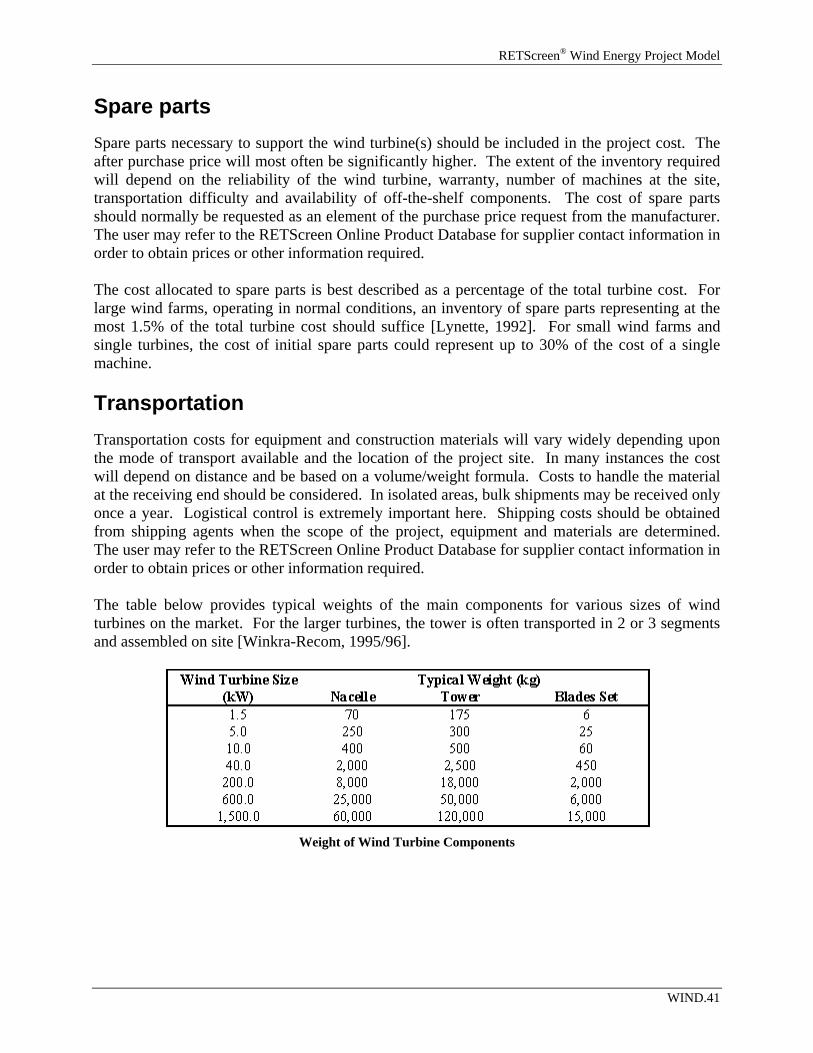
RETScreen® Wind Energy Project Model
Spare parts Spare parts necessary to support the wind turbine(s) should be included in the project cost. The after purchase price will most often be significantly higher. The extent of the inventory required will depend on the reliability of the wind turbine, warranty, number of machines at the site, transportation difficulty and availability of off-the-shelf components. The cost of spare parts should normally be requested as an element of the purchase price request from the manufacturer. The user may refer to the RETScreen Online Product Database for supplier contact information in order to obtain prices or other information required. The cost allocated to spare parts is best described as a percentage of the total turbine cost. For large wind farms, operating in normal conditions, an inventory of spare parts representing at the most 1.5% of the total turbine cost should suffice [Lynette, 1992]. For small wind farms and single turbines, the cost of initial spare parts could represent up to 30% of the cost of a single machine. Transportation Transportation costs for equipment and construction materials will vary widely depending upon the mode of transport available and the location of the project site. In many instances the cost will depend on distance and be based on a volume/weight formula. Costs to handle the material at the receiving end should be considered. In isolated areas, bulk shipments may be received only once a year. Logistical control is extremely important here. Shipping costs should be obtained from shipping agents when the scope of the project, equipment and materials are determined. The user may refer to the RETScreen Online Product Database for supplier contact information in order to obtain prices or other information required. The table below provides typical weights of the main components for various sizes of wind turbines on the market. For the larger turbines, the tower is often transported in 2 or 3 segments and assembled on site [Winkra-Recom, 1995/96].
Weight of Wind Turbine Components
WIND.41
RETScreen® Software Online User Manual
Other These input cells are provided to allow the user to enter cost or credit items that are not included in the information provided in the above cost category. The user must enter a positive numerical value in the "Unit Cost" column. A cost item may be entered in the grey input cell as "Other." The user then selects "Cost" from the drop-down list in the unit column. The user can input both a quantity amount and unit cost. This item is provided to allow for project, technology and/or regional differences not specifically covered in the generic information provided. A credit item may be entered in the grey input cell as "Credit." The user then selects "Credit" from the drop-down list in the unit column. The project may be credited for material and/or labour costs that would have been spent on the base case, or conventional, energy system. The user can input both a quantity amount and unit cost. Note that the credit item is expressed as a negative value in the "Amount" column. Balance of Plant The balance of plant for a wind energy project typically includes a number of items. These items include wind turbine(s) foundations(s) and erection, road construction, transmission line, substation, control and O&M building(s) and transportation costs. The user may refer to the RETScreen Online Product Database for supplier contact information in order to obtain prices or any other information required. These costs are detailed below. For a large wind farm, the balance of plant costs should fall between 17 and 26% of the total wind energy project cost. For a small wind farm, it should fall between 13 and 22%. In the case of a single turbine, this cost is highly dependent on the particular circumstances of the project.
Wind turbine(s) foundation(s) Wind turbine foundations include the labour and material, such as forms, concrete, steel frames and anchors, pilings and fabricated parts. The wind turbine foundations will be specific to the wind turbine and to the site. The manufacturer should be requested to provide design information and loads data for design of foundations. The user may refer to the RETScreen Online Product Database for supplier contact information in order to obtain prices or other information required. Cost estimates for foundations and materials should be requested from contractors in the project area. In some instances the type of foundations used in some areas will be much different than that which might be used in a community where the construction of concrete bases is a standard practice. Transportation of material could be a large portion of the cost. For large wind turbines, foundation costs typically fall between $10,000 and $50,000 per turbine. For medium wind turbines, it typically ranges between $7,000 to $25,000 per turbine. A more precise estimate can be obtained once the geotechnical surveys have been conducted. Foundation costs also depend on the number and exact size of the wind turbines, the type of tower used and
WIND.42
RETScreen® Wind Energy Project Model
the accessibility of the site. Hence, the costs suggested can be significantly higher for isolated project sites [Lynette, 1992] and [Reid, 1996]. For large wind farms, foundations typically represent 4 to 9% of the total renewable energy equipment and balance of plant costs [Conover, 1994] and [Vesterdal, 1992]. Wind turbine(s) erection Wind turbine erection includes labour and rental (or purchase) of equipment. The equipment required may vary from cranes and heavy vehicles to special winches, gin poles and other mechanical equipment specific to the wind turbine being considered. For isolated project sites it will usually be more cost-effective to rent tools and equipment, depending on availability, rather than to purchase and ship them in. Costs for rental equipment can be very high. Good planning is required. Many times deals can be worked for resale of equipment in the community after use if rental equipment is not available. The user will need to check for their availability and costs on a case by case basis. Often, the various construction contractors will include these costs in their bids so make sure not to double count those items here. Skilled labour to construct a large energy project may not be available in all project locations. The cost of skilled and unskilled labour in isolated areas is typically twice the rate found in populated areas. Productivity can often be considerably lower for a number of reasons, such as weather conditions, skills, etc. Travel costs will have to be added for labour required from outside the project area. For large wind farms, wind turbine(s) erection typically represents 4% of the total renewable energy equipment and balance of plant costs [Zond, 1994]. This proportion increases with small wind farm and single turbine installation, due to smaller economies of scale. Road construction An access road for construction and an on-going service road is normally required for a medium to large-scale wind energy project. These requirements will depend on the site selection and the nature of the terrain. There may be seasonal limitations both for construction activity and for use of roads to transport equipment. At some project sites there may be no need for road construction even if the site selected is not on existing routes. The location of existing roads is a consideration during site selection. Cost for road construction typically ranges from $0 to $80,000 per km, but can be as high as $500,000 per km if river crossings are required. The length of the road required comprises the length of the access road to the site and the length of the service road on the site, linking the turbines, if there is more than one turbine. The anticipated length of the required access and service roads can be determined by topographic maps. For large wind farms, roads typically represent 1 to 3% of total renewable energy equipment and balance of plant costs [Conover, 1994] and [Zond, 1994].
WIND.43
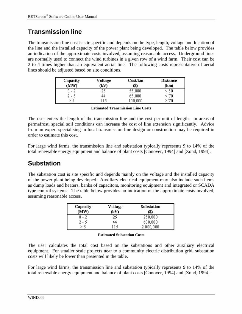
RETScreen® Software Online User Manual
Transmission line The transmission line cost is site specific and depends on the type, length, voltage and location of the line and the installed capacity of the power plant being developed. The table below provides an indication of the approximate costs involved, assuming reasonable access. Underground lines are normally used to connect the wind turbines in a given row of a wind farm. Their cost can be 2 to 4 times higher than an equivalent aerial line. The following costs representative of aerial lines should be adjusted based on site conditions.
Estimated Transmission Line Costs
The user enters the length of the transmission line and the cost per unit of length. In areas of permafrost, special soil conditions can increase the cost of line extension significantly. Advice from an expert specialising in local transmission line design or construction may be required in order to estimate this cost. For large wind farms, the transmission line and substation typically represents 9 to 14% of the total renewable energy equipment and balance of plant costs [Conover, 1994] and [Zond, 1994]. Substation The substation cost is site specific and depends mainly on the voltage and the installed capacity of the power plant being developed. Auxiliary electrical equipment may also include such items as dump loads and heaters, banks of capacitors, monitoring equipment and integrated or SCADA type control systems. The table below provides an indication of the approximate costs involved, assuming reasonable access.
Estimated Substation Costs
The user calculates the total cost based on the substations and other auxiliary electrical equipment. For smaller scale projects near to a community electric distribution grid, substation costs will likely be lower than presented in the table. For large wind farms, the transmission line and substation typically represents 9 to 14% of the total renewable energy equipment and balance of plant costs [Conover, 1994] and [Zond, 1994].
WIND.44
RETScreen® Wind Energy Project Model
Control and O&M building(s) A control building may or may not be necessary. Due to the costs of these buildings, the project developer should try to avoid this requirement where it is practical to do so. A control building may also serve as a location for maintenance work and storage of spare parts and materials. Modern wind turbines can be controlled remotely which may eliminate the need for such a facility. Existing utility locations may be possible alternatives. Construction costs for buildings will be very high in some communities. Usually a local builder will be able to give a quick estimate for the cost of a suitable new structure or for renovation of an existing space. For large-scale wind energy projects, the O&M/control building typically represents 1% of the total renewable energy equipment and balance of plant costs [Vesterdal, 1992]. Transportation Transportation costs for equipment and construction materials will vary widely depending upon the mode of transport available and the location of the project site. In many instances the cost will depend on distance and be based on a volume/weight formula. Costs to handle the material at the receiving end should be considered. In isolated areas, bulk shipments may be received only once a year. Logistical control is extremely important here. Shipping costs should be obtained from shipping agents when the scope of the project, equipment and materials are determined. Note that some cost items detailed above may include transportation costs when performed by local contractors so the user should be careful not to double count. Other These input cells are provided to allow the user to enter cost or credit items that are not included in the information provided in the above cost category. The user must enter a positive numerical value in the "Unit Cost" column. A cost item may be entered in the grey input cell as "Other." The user then selects "Cost" from the drop-down list in the unit column. The user can input both a quantity amount and unit cost. This item is provided to allow for project, technology and/or regional differences not specifically covered in the generic information provided. A credit item may be entered in the grey input cell as "Credit." The user then selects "Credit" from the drop-down list in the unit column. The project may be credited for material and/or labour costs that would have been spent on the base case, or conventional, energy system. The user can input both a quantity amount and unit cost. Note that the credit item is expressed as a negative value in the "Amount" column.
WIND.45

RETScreen® Software Online User Manual
Miscellaneous This category is for all of the miscellaneous costs that occur during a project and have not been taken into account in the previous sections. For wind energy projects these costs can include training, commissioning, contingencies and interest during construction. For a large wind farm, the miscellaneous costs, excluding contingencies, should fall between 1 and 4% of the total wind energy project cost. For a small wind farm, it should fall between 2 and 15%. In the case of a single turbine, this cost is highly dependent on the particular circumstances of the project. Training The costs associated with the training of plant operators and maintenance personnel will depend on the size, complexity and remoteness of the installation. For isolated areas, there will be a greater need for local trained technicians in order to avoid lengthy repair delays. For a large wind farm, up to 6 maintenance technicians per section of 50 wind turbines, in addition to 3 operators, may be required. For single turbines and small wind farms, one operator/maintenance technician can perform daily operation and maintenance tasks. However, some of the periodic repairs (e.g. gearbox replacement) will require specialised labour. Training costs include professional fees. Any travel expenses can be entered in "Travel and accommodation" under the "Development" section. Training will involve between 2 and 10 people for 1 to 20 days at a rate of between $200 and $800 per person-day depending on the size of the project. Commissioning Commissioning is the last activity of the construction phase. It consists of operating all the equipment to detect and fix any malfunctions, and ensure that the wind turbines and the wind farm function as guaranteed. Commissioning normally involves the monitoring of the wind plant performance over a set period of time under typical operating conditions. The cost associated with the commissioning of the wind farm will depend on the technology, size and number of turbines of the wind plant and on the skills and experience of the O&M staff. It could also depend on the climatic conditions to the extent that a sustained period of sufficient wind is required to prove the adequate performance of the equipment. Commissioning will involve between 1 and 8 people for 1 to 30 days at a rate of between $200 and $800 per person-day depending on the size of the project. Contingencies The allowance made for contingency costs depends on the level of accuracy of the cost estimates. Contingencies are estimated based on a user-selected percentage of the subtotal of all project
WIND.46
RETScreen® Wind Energy Project Model
costs excluding interest during construction. Note that contingencies are incremental in the sense that they are derived from project costs including any credits. The allowance for contingency items should be based on the level of accuracy associated with the RETScreen pre-feasibility estimate of the project costs. Typically, a pre-feasibility level cost analysis should be accurate within 40 to 50%. However, this accuracy will depend on the expertise of the study team, the scale of the project being considered, the level of effort put forward to complete the pre-feasibility study and the availability of accurate information. It is certainly possible that the RETScreen user experienced with wind energy project developments could estimate costs in the range of 5 to 40% of the total initial project costs. Interest during construction Interest during construction (short-term construction financing) will vary depending on the duration of construction and the cost of money. Although the construction of a wind farm can take up to one year, normally not more than 6 months are required between delivery of the turbines (the most important cost item) and commissioning of the wind farm. The user enters the interest rate (%) and the length of construction in months. The interest cost during construction is then calculated assuming the average debt over the project length in months is 50% of the subtotal of all project costs. For example, if $1 million worth of equipment must be financed over 12 months at an annual rate of 10%, the user should enter 10% as the interest rate during construction, the calculated interest cost during construction is: $1,000,000 x 50% x 12 months/12 months/year x 10% / year = $50,000. The cost of interest during construction can vary between 3 and 15% of the project costs. Annual Costs (Credits) There will be a number of annual costs associated with the operation of a wind energy project. These will include land lease, property taxes, insurance premium, transmission line maintenance, parts and labour, GHG monitoring and verification, community benefits, travel and accommodation and general and administrative expenses. In addition, costs for contingencies will also be incurred. These costs are detailed below. O&M
Land lease The user enters the applicable annual land lease costs. It is often necessary to negotiate the use of the land where the project is being implemented. In some cases an agreement may be established that a renewable energy project is a desirable use of the land and that no land use expenses will be charged to the project developer. As an example, this may be the case on government owned land. However, in most cases the landowner requires compensation for use of the land over a fixed period of time. Farmers, who can still use the land in and around the project site, are a common example.
WIND.47
RETScreen® Software Online User Manual
As a rule-of-thumb, the annual cost of leasing the land for a wind energy project typically ranges between 1 and 5% of project capacity and energy revenues [Conover, 1994], [Johansson, 1993], [Zond, 1994] and [Gipe, 1995]. Property taxes This cost item summarises the annual costs of property taxes and is calculated as a percentage of the total estimated initial costs. Property tax might be levied on a wind energy project, depending upon the jurisdiction. Applicable property taxes have to be estimated on a site-by-site basis and will depend on the property value of the project and/or the revenue generated by the project. As a rule-of-thumb, the annual cost of property taxes for a wind energy project represents 0 to 2% of project capacity and energy revenues. Insurance premium This cost item summarises the annual insurance premium costs and is calculated as a percentage of the total estimated initial costs. As a minimum, insurance is required for public liability, property damage, equipment failure and business interruption. The annual costs for insurance can be significant for an energy project and should be estimated by contacting an insurance broker. As a rule-of-thumb, the annual cost of insurance for a wind energy project can range between 2 and 4% of project capacity and energy revenues [Conover, 1994] and [Zond, 1994]. Transmission line maintenance The user enters the percentage of capital costs associated with transmission line maintenance costs. The maintenance of transmission lines associated with a wind energy project will involve periodic clearing of trees (where present) and replacement of parts (e.g. poles, conductor, insulators) that become damaged due to lightning, impact, etc. The annual cost of transmission line maintenance is estimated based on the capital cost of the transmission line and substation. Annual costs normally range between 3 and 6% of capital costs depending on the location and communication equipment required (i.e. ease of access, presence of trees, VHF radio network, etc.). Parts and labour The parts and labour cost item summarises the cost of spare parts and annual labour required for routine and emergency maintenance and operation of the wind turbine(s). Operation includes monitoring, regular inspection of the equipment (including routine lubrication and adjustments), snow, ice and dirt removal, scheduled maintenance (internal inspection and maintenance of the turbine(s)), etc.
WIND.48
RETScreen® Wind Energy Project Model
Labour costs in isolated areas are typically twice the rate found in most central locations. Productivity is often much less. The rates proposed below should thus be adjusted accordingly if appropriate. The cost for parts and labour is best expressed in terms of dollars per kWh produced by the wind energy project. For a large wind farm, this cost falls between 0.007 and 0.024 $/kWh with an average around 0.014 $/kWh [Gipe, 1995]. For small wind farms and single turbines, a cost of 0.015 $/kWh is a reasonable first approximation. GHG monitoring and verification Greenhouse gas (GHG) monitoring is generally carried out by project proponents in accordance with the data requirements and methods laid out in the Monitoring Plan. If additional data needs to be collected in order to estimate GHG emissions, the cost of collecting that data and quantifying emissions reductions should be estimated. Note that in the case of Clean Development Mechanism (CDM) projects sustainable development indicators will also need to be monitored. For small-scale CDM projects (15 MW or less), monitoring requirements will be simplified, and therefore the estimated costs should be reduced. (See UNFCCC's CDM Website for details on monitoring requirements for CDM projects.) Most GHG projects will also require third party verification of emissions reductions on an annual or periodic basis. For Joint Implementation (JI) projects, verification results in an independent confirmation of the actual emissions reductions the project has achieved and the quantification of Emissions Reduction Units (ERUs). For CDM projects, emissions reductions must be verified and certified by a designated operational entity before Certified Emissions Reductions (CERs) are issued. A prescribed rate of $US 400/day has been set for the staff of designated operational entities or $US 1,200/day for a team of three. For CDM projects, an administration and adaptation fee will be charged by the United Nations Framework Convention on Climate Change (UNFCCC). Some host countries may also require a percentage of the value of CERs to be paid as an administration fee (note this percentage can be entered and accounted for on the GHG Analysis worksheet). It may be decided to bundle and incur GHG monitoring and verification on a periodic (e.g. every two years) rather than on an annual basis, especially for smaller projects. In this case, the user should use the Periodic Costs section at the bottom of the Cost Analysis worksheet to do so, and set the same to "0" in the Annual O&M Costs section. Community benefits In order to ensure the acceptance of a wind project within a community, it is common in large projects to reserve a small portion of the O&M budget to fund an initiative that will benefit the community. This could take the form of a donation to support a public awareness centre for the wind farm, donations to charitable organisations, a grant to support cultural or sporting events, scholarships, training sessions, environmental protection, etc.
WIND.49
RETScreen® Software Online User Manual
Travel and accommodation For wind energy systems in isolated locations, an annual allowance should be made for travel, room and board costs associated with annual maintenance. General and administrative Annual general and administrative costs include the costs of bookkeeping, preparation of annual statements, bank charges, communication, etc. General and administrative costs are project specific and depend on the nature of the business enterprise (e.g. privately-owned with a simple power purchase agreement or utility/publicly owned with individual customers). General and administrative costs can range between 1 to 20% of the annual costs (excluding other costs and contingencies). Other These input cells are provided to allow the user to enter cost or credit items that are not included in the information provided in the above cost category. The user must enter a positive numerical value in the "Unit Cost" column. A cost item may be entered in the grey input cell as "Other." The user then selects "Cost" from the drop-down list in the unit column. The user can input both a quantity amount and unit cost. This item is provided to allow for project, technology and/or regional differences not specifically covered in the generic information provided. A credit item may be entered in the grey input cell as "Credit." The user then selects "Credit" from the drop-down list in the unit column. The project may be credited for material and/or labour costs that would have been spent on the base case, or conventional, energy system. The user can input both a quantity amount and unit cost. Note that the credit item is expressed as a negative value in the "Amount" column. Contingencies A contingency allowance should be included to account for unforeseen annual expenses and will depend on the level of accuracy of the operation and maintenance cost estimate section. This is especially true in the case of project in isolated areas. It is common to carry a contingency allowance for at least the replacement of the most expensive component subject to catastrophic failure. The contingency allowance is calculated based on an estimated percentage of the other operation and maintenance costs. It typically ranges from 10 to 20% of these costs. Periodic Costs (Credits) This section is provided to allow the user to specify the periodic costs associated with the operation of the system over the project life. Grey input cells are provided to allow the user to
WIND.50
RETScreen® Wind Energy Project Model
enter the name of a periodic cost and periodic credit item. The user must enter a positive numerical value in the "Unit Cost" column. A periodic cost represents recurrent costs that must be incurred at regular intervals to maintain the project in working condition. A periodic cost item is entered in the grey input cell. The user then selects "Cost" from the drop-down list in the unit column. The interval (in years) over which the periodic cost is incurred is entered in the period column. The amount of the cost incurred at each interval is entered in the unit cost column. The project may also be credited for periodic costs that would have been incurred over the project life of the base case, or conventional, energy system. The periodic credit item is entered in the grey input cell. The user then selects "Credit" from the drop-down list in the unit column. The interval (in years) over which the periodic credit is incurred is entered in the period column. The amount of the credit incurred at each interval is entered in the unit cost column. Note that the credit item is expressed as a negative value in the "Amount" column. End of project life The user enters the value of the project at the end of its life. This amount is also commonly referred to as the salvage value (or disposal value). If the salvage value of the project at the end of its life is positive, then the user selects "Credit" from the drop-down list in the unit column in order to express this item as a negative value. However, if the costs of remediation or decommissioning that must be incurred at the end of the project life exceed the salvage value, then the user must select "Cost" from the drop-down list. The user must enter a positive numerical value in the "Unit Cost" column. Note: At this point, the user should go to the optional GHG Analysis worksheet.
WIND.51
RETScreen® Software Online User Manual
Financial Summary As part of the RETScreen Clean Energy Project Analysis Software, a Financial Summary worksheet is provided for each project evaluated. This common financial analysis worksheet contains five sections: Annual Energy Balance, Financial Parameters, Project Costs and Savings, Financial Feasibility and Yearly Cash Flows. The Annual Energy Balance and the Project Costs and Savings sections provide a summary of the Energy Model, Cost Analysis and GHG Analysis worksheets associated with each project studied. In addition to this summary information, the Financial Feasibility section provides financial indicators of the project analysed, based on the data entered by the user in the Financial Parameters section. The Yearly Cash Flows section allows the user to visualise the stream of pre-tax, after-tax and cumulative cash flows over the project life. The Financial Summary worksheet of each Workbook file has been developed with a common framework so as to simplify the task of the user in analysing the viability of different projects. This also means the description of each parameter is common for most of the items appearing in the worksheet. One of the primary benefits of using the RETScreen software is that it facilitates the project evaluation process for decision-makers. The Financial Summary worksheet, with its financial parameters input items (e.g. avoided cost of energy, discount rate, debt ratio, etc.), and its calculated financial feasibility output items (e.g. IRR, simple payback, NPV etc.), allows the project decision-maker to consider various financial parameters with relative ease. A description of these items, including comments regarding their relevance to the preliminary feasibility analysis, is included below. Annual Energy Balance The summary items here are calculated and/or entered in the Energy Model and GHG Analysis worksheets and transferred to the Financial Summary worksheet. Project name The user-defined project name is entered for reference purposes only in the Energy Model worksheet, and it is copied automatically to the Financial Summary worksheet. Project location The user-defined project location is entered for reference purposes only in the Energy Model worksheet, and it is copied automatically to the Financial Summary worksheet. Renewable energy delivered The Energy Model calculates the annual renewable energy production (MWh) of the project. This renewable energy delivered by the project also equates to the annual energy savings as compared with the base case electricity system. For central-grid applications, all the energy produced is assumed to be absorbed by the grid.
WIND.52
RETScreen® Wind Energy Project Model
For isolated-grid and off-grid applications, all the energy produced might not be absorbed by the grid due to a mismatch between energy demand and the energy supply. The model does not consider storage of excess renewable energy. In this case, the renewable energy delivered equals the renewable energy collected less the excess energy available. Excess RE available For "Isolated-grid" and "Off-grid" grid types, the Energy Model calculates the excess renewable energy available (MWh), which is the energy from the renewable energy system that is not absorbed by the grid or off-grid load and, therefore, is available as a by-product for heating or other uses. Firm RE capacity The firm RE capacity refers to the "guaranteed" electrical power (kW) that a renewable energy electric power project can deliver. For wind energy projects, which are inherently intermittent, the user enters an "avoided cost of capacity" that is agreed upon with (may need to be negotiated) the local electric utility. This avoided cost of capacity will depend upon the profile of the local electrical demand and renewable energy supply conditions. In the most conservative cases, due to the intermittent nature of wind energy resources, the firm renewable energy capacity value would equal 0. Grid type The grid type is selected in the Energy Model worksheet, and it is copied automatically to the Financial Summary worksheet. Peak load For "Isolated-grid" and "Off-grid" grid types, the peak electrical load (kW) of the local electric utility (or application for off-grid systems) is entered in the Energy Model worksheet, and it is copied automatically to the Financial Summary worksheet. This is the peak load faced during the year. Net GHG emission reduction - credit duration The model calculates the cumulative net greenhouse gas (GHG) emission reduction for the duration of the GHG credit, in equivalent tonnes of CO2 (tCO2), resulting from the implementation of the project instead of the base case, or baseline, system. This value is calculated by multiplying the appropriate net annual GHG emission reduction by the GHG reduction credit duration. Net GHG emission reduction [ yr 1 to x (1st period)] The model calculates the net annual average GHG emission reduction in equivalent tonnes of CO2 per year (tCO2/yr) resulting from the implementation of the project instead of the base case,
WIND.53
RETScreen® Software Online User Manual
or baseline, system. This value is calculated in the GHG Analysis worksheet and it is copied automatically to the Financial Summary worksheet. For projects in which a change in baseline emission factor has been selected in the GHG Analysis worksheet, the model indicates the net annual average GHG emission reduction for the years preceding the change.
Net GHG emission reduction - yr x+1 and beyond (2nd period) The model calculates the net annual average GHG emission reduction in equivalent tonnes of CO2 per year (tCO2/yr) resulting from the implementation of the project instead of the base case, or baseline, system, for the years following the change in baseline emission factor. This value is calculated in the GHG Analysis worksheet, and it is copied automatically to the Financial Summary worksheet.
Net GHG emission reduction - project life The model calculates the cumulative net GHG emission reduction for the duration of the project life, in equivalent tonnes of CO2 (tCO2), resulting from the implementation of the project instead of the base case, or baseline, system. This value is calculated by multiplying the appropriate net annual GHG emission reduction by the project life.
Financial Parameters The items entered here are used to perform calculations in this Financial Summary worksheet. Values for each parameter will depend on the perspective of the user (e.g. electric utility vs. independent power producer). Avoided cost of energy The user enters the avoided cost of energy per kWh. This value typically represents either the "average" or the "marginal" unit cost of energy for the base case electricity system and is directly related to the cost of fuel for the base case electricity system. The user is given the flexibility in the model to determine what the base case electricity system is. For example, the base case energy costs being avoided may be for a new combined-cycle natural gas fired power plant established as a "proxy" or baseline reference case by the local utility. The user will need to determine this value. Avoided cost of energy calculations for electric power generation usually require a relatively detailed analysis [Leng, 1993]. For electric power generation, electric utilities will normally calculate this value for their service area. This value may also be the amount that utilities might pay independent power producers (IPP) for electricity produced by the IPP. Utilities might assign a higher value where distributed generation benefits are obtainable [Leng, 1994]. A more detailed description is beyond the scope of this manual (for a more detailed description see Johansson, 1993). However, a brief description of possible values follows.
WIND.54
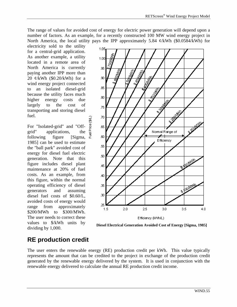
RETScreen® Wind Energy Project Model
The range of values for avoided cost of energy for electric power generation will depend upon a number of factors. As an example, for a recently constructed 100 MW wind energy project in North America, the local utility pays the IPP approximately 5.84 ¢/kWh ($0.0584/kWh) for electricity sold to the utility for a central-grid application. As another example, a utility located in a remote area of North America is currently paying another IPP more than 20 ¢/kWh ($0.20/kWh) for a wind energy project connected to an isolated diesel-grid because the utility faces much higher energy costs due largely to the cost of transporting and storing diesel fuel. For "Isolated-grid" and "Off-grid" applications, the following figure [Sigma, 1985] can be used to estimate the "ball park" avoided cost of energy for diesel fuel electric generation. Note that this figure includes diesel plant maintenance at 20% of fuel costs. As an example, from this figure, within the normal operating efficiency of diesel generators and assuming diesel fuel costs of $0.60/L, avoided costs of energy would range from approximately $200/MWh to $300/MWh. The user needs to correct these values to $/kWh units by dividing by 1,000.
Diesel Electrical Generation Avoided Cost of Energy [Sigma, 1985]
RE production credit The user enters the renewable energy (RE) production credit per kWh. This value typically represents the amount that can be credited to the project in exchange of the production credit generated by the renewable energy delivered by the system. It is used in conjunction with the renewable energy delivered to calculate the annual RE production credit income.
WIND.55
RETScreen® Software Online User Manual
RE production credits are most common for electricity generation from renewable energy projects. For example, it is possible to receive a tax credit of 1.5 ¢/kWh in the USA for electricity produced from wind, biomass or chicken manure. Whether or not a given project would qualify to receive such payments depends on the rules of the specific programs in the jurisdiction in which the system is installed. The value entered is assumed to be representative of year 0, i.e. the development year prior to the first year of operation (year 1). For tax purposes, the RE production credit is treated as supplemental income. The model escalates the RE production credit value yearly according to the RE credit escalation rate starting from year 1 and throughout the RE production credit duration. RE production credit duration The user enters the renewable energy (RE) production credit duration (year). This value typically represents the number of years for which the project receives a RE production credit. It is used to calculate the annual RE production credit income. RE credit escalation rate The user enters the renewable energy (RE) credit escalation rate (%), which is the projected annual average rate of increase in the renewable energy credit over the RE production credit duration. This allows the user to apply rates of inflation to the value of renewable energy production credits which may be different from general inflation. GHG emission reduction credit The user enters the GHG emission reduction credit per tonne of CO2 (tCO2). It is used in conjunction with the net GHG emission reduction to calculate the annual GHG emission reduction income. Preliminary estimates predict the market price of GHG emission reduction credits in the USA will range from $US 4 to $US 95 per tonne of CO2, with $ 5 to $ 8 per tonne being the most likely range [Sandor, 1999]. As of 2003, the global market price has typically been in the range of $US 3 to $US 5 per tonne of CO2. The value entered is assumed to be representative of year 0, i.e. the development year prior to the first year of operation (year 1). The model escalates the GHG emission reduction credit value yearly according to the GHG credit escalation rate starting from year 1 and throughout the project life. GHG reduction credit duration The user enters the GHG reduction credit duration (year). This value typically represents the number of years for which the project receives GHG reduction credits. It is used to determine the annual GHG reduction income.
WIND.56
RETScreen® Wind Energy Project Model
For Clean Development Mechanism (CDM) projects, two options are available for the length of the crediting period (i) a fixed crediting period of 10 years or (ii) a renewable crediting period of 7 years that can be renewed twice (for a maximum credit duration of 21 years). If a crediting period of 10 years is selected, once the project has been validated and registered, Certified Emission Reductions (CERs) can be certified and issued for the 10 years of the project without revisiting the baseline. However, in the case of a renewable 7 year crediting period, the project will have to be validated after each 7 year period in order to receive CERs for the subsequent 7 years. Thus in selecting a crediting period, the benefits of the potentially longer crediting period of the renewable crediting period (e.g. up to 21 years) must be weighed against the additional transaction costs of re-validating the project after each 7 year period, and the risk of the project potentially not meeting validation requirements at that time. GHG credit escalation rate The user enters the GHG credit escalation rate (%), which is the projected annual average rate of increase in the GHG emission reduction credit over the life of the project. This permits the user to apply rates of inflation to the market price of GHG emission reduction credits which may be different from general inflation. Avoided cost of excess energy The user enters the avoided cost of excess energy per kWh. The avoided cost of excess energy may range from zero, where there is no need for the excess energy, to a value close to the local retail price for electricity. Avoided cost of capacity The user enters the avoided cost of capacity per kW-yr. Unless the user knows this value, it is safer to assume a zero for this entry as this number is often incorporated into the "avoided cost of energy" value. If the project being evaluated has a zero "Firm RE capacity" then this item is hidden in the spreadsheet. The value of avoided cost of capacity typically represents either the "average" or the "marginal" unit cost of capacity for a base case electric power system. This value is directly related to the cost of generation capacity for the base case electricity system. Avoided cost of capacity calculations for electric power generation usually requires a relatively detailed analysis. For electric power generation, electric utilities will normally calculate this value for their service area. This value may also be the amount that utilities will pay IPPs for electric capacity provided to the utility. Utilities may assign a higher value where distributed generation benefits are obtainable to account for Transmission and Distribution (T&D) capacity attributes [Leng, 1994]. A more detailed description is beyond the scope of this manual (for a more detailed description, see Johansson, 1993). As a brief example, a New England electric utility has valued avoided capacity costs at roughly $100/kW-yr for a proxy gas turbine and marginal avoided T&D costs at $250/kW-yr for central-grid applications [Leng, 1993].
WIND.57
RETScreen® Software Online User Manual
Energy cost escalation rate The user enters the energy cost escalation rate (%), which is the projected annual average rate of increase for the avoided cost of energy over the life of the project. This permits the user to apply rates of inflation to energy costs which are different from general inflation for other costs. For example, North American electric utilities currently use energy cost escalation rates ranging anywhere from 0 to 5% with 2 to 3% being the most common values. Inflation The user enters the inflation rate (%), which is the projected annual average rate of inflation over the life of the project. For example, inflation for the next 25 years in North America is currently forecasted to range between 2 and 3%. Discount rate The user enters the discount rate (%), which is the rate used to discount future cash flows in order to obtain their present value. The rate generally viewed as being most appropriate is an organisation's weighted average cost of capital. An organisation's cost of capital is not simply the interest rate that it must pay for long-term debt. Rather, cost of capital is a broad concept involving a blending of the costs of all sources of investment funds, both debt and equity. The discount rate used to assess the financial feasibility of a given project is sometimes called the "hurdle rate," the "cut-off rate," or the "required rate of return." The model uses the discount rate to calculate the annual life cycle savings. For example, North American electric utilities currently use discount rates ranging anywhere from 3 to 18% with 6 to 11% being the most common values. Project life The user enters the project life (year), which is the duration over which the financial feasibility of the project is evaluated. Depending on circumstances, it can correspond to the life expectancy of the energy equipment, the term of the debt, or the duration of a power purchase agreement. Although the model can analyse project life's up to 50 years, the project life of a well designed wind energy project typically falls between 20 and 30 years. Debt ratio The user enters the debt ratio (%), which is the ratio of debt over the sum of the debt and the equity of a project. The debt ratio reflects the financial leverage created for a project; the higher the debt ratio, the larger the financial leverage. The model uses the debt ratio to calculate the equity investment that is required to finance the project. For example, debt ratios typically range anywhere from 0 to 90% with 50 to 90% being the most common.
WIND.58
RETScreen® Wind Energy Project Model
Debt interest rate The user enters the debt interest rate (%), which is the annual rate of interest paid to the debt holder at the end of each year of the term of the debt. The model uses the debt interest rate to calculate the debt payments. For example, at a minimum the debt interest rate will correspond to the yield of government bonds with the same term as the debt term. A premium is normally added to this rate (the "spread") to reflect the perceived risk of the project. Debt term The user enters the debt term (year), which is the number of years over which the debt is repaid. The debt term is either equal to, or shorter than the project life. Generally, the longer the term, the more the financial viability of an energy project improves. The model uses the debt term in the calculation of the debt payments and the yearly cash flows. The term of the debt normally falls within a 1 to 25 year range. It should not exceed the estimated project life. Income tax analysis The user indicates by selecting from the drop-down list whether or not income tax should be factored into the financial analysis. If the user selects "Yes" certain input fields will be added to allow the user to customise the income tax analysis according to the specific circumstances of the project. In some situations, the after-tax return of a project can be more attractive than its pre-tax return. The income tax analysis allows the model to calculate after-tax cash flows and after-tax financial indicators. In all cases, the model assumes a single income tax rate valid throughout the project life and applied to net income. Note that the analysis is based, among others, on net initial and annual costs, i.e. any credits entered in the Cost Analysis worksheet for these two categories are not treated separately. This leads to a reasonably accurate tax analysis unless the initial and/or annual credits are of the same order of magnitude as the corresponding costs and fall under a different depreciation schedule for tax purposes. Effective income tax rate The user enters the effective income tax rate (%), which is the effective equivalent rate at which the net income derived from the project is taxed. For example, in most jurisdictions, this would correspond to the combined federal, provincial /state and/or local income tax rates for businesses. Net taxable income is derived from the project cash inflows and outflows assuming that all revenues and expenses are paid at the end of the year in which they are earned or incurred. The effective income tax rate is assumed to be constant throughout the project life. Note that sales tax should be considered in the "Initial Costs" section of the Cost Analysis worksheet and that property tax should be considered in the "Annual Costs" section.
WIND.59
RETScreen® Software Online User Manual
Loss carryforward? The user indicates by selecting from the drop-down list whether or not losses are carried forward, i.e. whether or not a loss (a negative taxable income) in a given year can be used to lower taxes owed in that same year or can be deferred to offset profits from future years. If the user selects "Yes," losses are carried forward and applied against taxable income in the following years, thereby reducing the income tax owed up to the accumulated losses, years after the losses occur. If the user selects "No," losses are not carried forward but rather lost and thereby never used to offset any other year taxable income. If the user selects "Flow-through," losses are not carried forward but rather used in the year in which they occur and applied against profits from sources other than the project (or qualify and generate a refundable tax credit), thereby reducing the income tax owed in the years in which losses occur. Whether losses must be carried forward or not will depend on the tax laws in the jurisdiction in which the project is located. The "Flow-through" situation is typically the most advantageous for the project owner and can contribute to make profitable a project which would not appear financially attractive on a pre-tax basis. The model does not allow losses to be carried backward and does not set a limit on the number of years for carryforwards. Depreciation method The user selects the depreciation method from three options in the drop-down list: "None," "Declining balance" and "Straight-line." This selection of the yearly depreciation of assets is used in the model in the calculation of income taxes and after-tax financial indicators. The user should select the method accepted by the tax departments in the jurisdiction of the project. The difference between the "End of project life" value and its undepreciated capital costs at the end of the project life is treated as income if positive and as a loss if negative. When "None" is selected, the model assumes that the project is fully capitalised at inception, is not depreciated through the years and therefore maintains its undepreciated value throughout its life. When "Declining balance" is selected, the model assumes that the capitalised costs of the project, as specified by the depreciation tax basis, are depreciated at the depreciation rate. The portion of initial costs not capitalised is deemed to be expensed during the year of construction, i.e. year 0. When "Straight line" is selected, the model assumes that the capitalised costs of the project, as specified by the depreciation tax basis, are depreciated with a constant rate over the depreciation period. The portion of initial costs not capitalised is deemed to be expensed during the year of construction, i.e. year 0. For both declining balance and straight-line depreciation, the model assumes that the full depreciation allowed for a given year is always taken. Also, the model does not incorporate the
WIND.60
RETScreen® Wind Energy Project Model
half-year rule used in some countries and according to which depreciation is calculated over only half of the capitalised cost during the first year of operation of the equipment. Depreciation tax basis The user enters the depreciation tax basis (%), which is used to specify which portion of the initial costs are capitalised and can be depreciated for tax purposes. The remaining portion is deemed to be fully expensed during the year of construction (year 0). For example, if a project costs $20,000 to evaluate (feasibility study) and develop, and $80,000 to design (engineering), build, install and commission, the user could enter 80% as the depreciation tax basis in order to depreciate only the engineering, energy equipment, balance of plant and miscellaneous costs while the feasibility and development costs would be fully expensed during year 0. Depreciation rate The user enters the depreciation rate (%), which is the rate at which the undepreciated capital cost of the project is depreciated each year. The depreciation rate can vary widely according to the class of assets considered and the jurisdiction in which the project is located. Depreciation period The user enters the depreciation period (year), which is the period over which the project capital costs are depreciated using a constant rate. The depreciation period can vary widely according to the class of assets considered and the jurisdiction in which the project is located. Tax holiday available? The user indicates by selecting from the drop-down list whether or not the project can benefit from a tax holiday. If the user selects "Yes," the tax holiday applies starting in the first year of operation, year 1, up to the tax holiday duration. The income tax calculation for the development/construction year, year 0, is not affected. Tax holiday duration The user enters the tax holiday duration (year), which is the number of years over which the tax holiday applies, starting in the first year of operation, year 1. For example, in India, certain renewable energy projects are given a five-year tax holiday. Project Costs and Savings Most of the summary items here are calculated and/or entered in the Cost Analysis worksheet and transferred to the Financial Summary worksheet. Some calculations are made in the Financial Summary worksheet.
WIND.61
RETScreen® Software Online User Manual
Initial Costs The total initial costs represent the total investment that must be made to bring a project on line, before it begins to generate savings (or income). The total initial costs are the sum of the estimated feasibility study, development, engineering, energy equipment, balance of plant and miscellaneous costs and are inputs in the calculation of the simple payback, the net present value and the project equity and debt. It is important to note that the range of possible costs listed throughout RETScreen do not include sales taxes. In a number of jurisdictions, clean energy project costs are often exempt from sales taxes. Users will have to consider these costs for their region when preparing their evaluations. For example, if in a particular region sales tax is applicable to the cost of an energy project then the user must add the amount of sales tax to the cost of the project chosen from the proposed range of values. Feasibility study The feasibility study item represents the sum of the costs incurred to assess the feasibility of a project. It is net of any "credits" for not having to develop the base case project. Considerable detail is provided in the Cost Analysis worksheet for estimating the sub-costs for feasibility studies. This is done because it will help the project proponent better estimate the costs of the next investment required, which is the investment in a feasibility study. However for smaller projects, the RETScreen analysis may be sufficient to move to the development and engineering phase or to construction. Note: The RETScreen Clean Energy Project Analysis Software can also be used to prepare the Feasibility Study. Development The development item typically represents the sum of the costs incurred to bring a project to the detailed design and construction stage, once its feasibility has been proven. It is net of any "credits" for not having to develop the base case project. Engineering The engineering item typically represents the sum of the costs of the design activities required to go from the development stage to the construction stage of a project. It is net of any "credits" for not having to develop the base case project. Energy equipment The energy equipment item typically represents the sum of the purchasing and installation costs of the energy equipment, less any "credits" for not having to purchase or install base case equipment.
WIND.62
RETScreen® Wind Energy Project Model
Balance of plant The balance of plant item represents the sum of the purchasing, construction and installation costs of all the elements of the energy system other than the energy equipment costs less any "credits" for not having to purchase or install base case equipment. Miscellaneous The miscellaneous item includes all the costs not considered in any of the other initial costs categories that are required to bring a project to the operational stage. Incentives/Grants The user enters the financial incentive; this is any contribution, grant, subsidy, etc. that is paid for the initial cost of the project. The incentive is deemed not to be refundable and is treated as income during the development/construction year, year 0, for income tax purposes. Annual Costs and Debt The total annual costs are calculated by the model and represent the yearly costs incurred to operate, maintain and finance the project. It is the sum of the O&M costs and debt payments. Note that the total annual costs include the reimbursement of the "principal" portion of the debt which is not, strictly speaking, a cost but rather an outflow of cash. These costs are described briefly below. O&M The operation and maintenance (O&M) costs are the sum of the annual costs that must be incurred to operate and maintain the energy system, in excess of the O&M cost required by the base case system. The model uses the O&M cost to calculate the total annual costs and the yearly cash flows. Debt payments - debt term The model calculates the debt payments, which is the sum of the principal and interest paid yearly to service the debt. Whereas debt payments are constant over the debt term, the principal portion increases and the interest portion decreases with time. In that respect, it is similar to the yearly annuity paid to reimburse the mortgage of a house. Debt payments are calculated using the debt interest rate, the debt term and the project debt. Annual Savings or Income The total annual savings represent the yearly savings realised due to the implementation of the project. From the perspective of an independent power producer these "savings" will be viewed
WIND.63
RETScreen® Software Online User Manual
as "income." It is directly related to the avoided cost of energy derived from implementing the project. It is an input in the calculation of the simple payback and the debt service coverage. Energy savings/income The annual energy savings are equal to the sum of the product of the "Renewable energy delivered" and "Avoided cost of energy" and, for isolated-grid and off-grid systems, the product of the "Excess RE available" and the "Avoided cost of excess energy." The yearly value of energy savings is escalated at the energy cost escalation rate. Capacity savings/income The annual capacity savings are equal to the product of the "Firm RE capacity" and the "Avoided cost of capacity." The yearly value of capacity savings is escalated at the inflation rate. RE production credit income - duration The model calculates the RE production credit income, which represents the income (or savings) generated by the sale or exchange of the RE production credits during the RE production credit duration. It is calculated from the renewable energy delivered and the RE production credit value. The yearly value of RE production credit income is escalated at the RE credit escalation rate. GHG reduction income - duration The model calculates the GHG emission reduction income which represents the income (or savings) generated by the sale or exchange of the GHG emission reduction credits. It is calculated from the annual net GHG emission reduction and the GHG emission reduction credit value. The yearly value of GHG emission reduction income is escalated at the GHG credit escalation rate. Periodic Costs (Credits) The periodic costs and periodic credits entered by the user in the Cost Analysis worksheet are transferred here. The model escalates the periodic costs and credits yearly according to the inflation rate starting from year 1 and throughout the project life. From an income tax perspective, periodic costs and credits are treated as operating expenses rather than capital investments and are therefore fully expensed in the year they are incurred. End of project life - Cost/Credit The value of the project at the end of its life entered by the user in the Cost Analysis worksheet is transferred here. This amount is also commonly referred to as the salvage value (or disposal value).
WIND.64
RETScreen® Wind Energy Project Model
The salvage value entered is assumed to be representative of year 0, i.e. the development/construction year prior to the first year of operation (year 1). The model escalates the salvage value yearly according to inflation rate starting from year 1 and up to the end of the project life (i.e. the schedule year reported in the model). For tax purposes, the difference between the project salvage value and its undepreciated capital costs at the end of the project life is treated as income if positive and as a loss if negative. Financial Feasibility The results provide the decision-maker with various financial indicators for the proposed project. Pre-tax Internal Rate of Return and Return on Investment The model calculates the pre-tax internal rate of return (%), which represents the true interest yield provided by the project equity over its life before income tax. It is also referred to as the return on investment (equity) (ROI) or the time-adjusted rate of return. It is calculated by finding the discount rate that causes the net present value of the project to be equal to zero. Hence, it is not necessary to establish the discount rate of an organisation to use this indicator. An organisation interested in a project can compare the internal rate of return of the project to its required rate of return (often, the cost of capital). The IRR is calculated on a nominal basis, that is including inflation. If the internal rate of return of the project is equal to or greater than the required rate of return of the organisation, then the project will likely be considered financially acceptable (assuming equal risk). If it is less than the required rate of return, the project is typically rejected. An organisation may have multiple required rates of return that will vary according to the perceived risk of the projects. The most obvious advantage of using the internal rate of return indicator to evaluate a project is that the outcome does not depend on a discount rate that is specific to a given organisation. Instead, the IRR obtained is specific to the project and applies to all investors in the project. The model uses the pre-tax yearly cash flows and the project life to calculate the internal rate of return. After-tax Internal Rate of Return and Return on Investment The model calculates the after-tax internal rate of return (%), which represents the true interest yield provided by the project equity over its life. It is also referred to as the return on investment (equity) (ROI) or the time-adjusted rate of return. It is calculated by finding the discount rate that causes the net present value of the project to be equal to zero. Hence, it is not necessary to establish the discount rate of an organisation to use this indicator. An organisation interested in a project can compare the internal rate of return of the project to its required rate of return (often, the cost of capital). The IRR is calculated on a nominal basis, that is including inflation. If the internal rate of return of the project is equal to or greater than the required rate of return of the organisation, then the project will likely be considered financially acceptable (assuming equal risk). If it is less than the required rate of return, the project is typically rejected. An organisation
WIND.65
RETScreen® Software Online User Manual
may have multiple required rates of return that will vary according to the perceived risk of the projects. The most obvious advantage of using the internal rate of return indicator to evaluate a project is that the outcome does not depend on a discount rate that is specific to a given organisation. Instead, the IRR obtained is specific to the project and applies to all investors in the project. The model uses the after-tax yearly cash flows and the project life to calculate the internal rate of return. Simple Payback The model calculates the simple payback (year), which represents the length of time that it takes for an investment project to recoup its own initial cost, out of the cash receipts it generates. The basic premise of the payback method is that the more quickly the cost of an investment can be recovered, the more desirable is the investment. For example, in the case of the implementation of a wind energy project, a negative payback period would be an indication that the annual costs incurred are higher than the annual savings generated. The simple payback method is not a measure of how profitable one project is compared to another. Rather, it is a measure of time in the sense that it indicates how many years are required to recover the investment for one project compared to another. The simple payback should not be used as the primary indicator to evaluate a project. It is useful, however, as a secondary indicator to indicate the level of risk of an investment. A further criticism of the simple payback method is that it does not consider the time value of money, nor the impact of inflation on the costs. On the other hand, the payback period is often of great importance to smaller firms that may be cash poor. When a firm is cash poor, a project with a short payback period, but a low rate of return, might be preferred over another project with a high rate of repayment, but a long payback period. The reason is that the organisation might simply need a faster return of its cash investment. The model uses the total initial costs, the total annual costs (excluding debt payments) and the total annual savings, in order to calculate the simple payback. The calculation is based on pre-tax amounts and includes any initial cost incentives. Year-to-positive cash flow The model calculates the number of years to positive (cumulative) cash flow, which represents the length of time that it takes for the owner of a project to recoup its own initial investment out of the project cash flows generated. The year-to-positive cash flow considers project cash flows following the first year as well as the leverage (level of debt) of the project, which makes it a better time indicator of the project merits than the simple payback. The model uses the year number and the cumulative after-tax cash flows in order to calculate this value. The year-to-positive cash flow differs from the discounted payback indicator in that it considers the nominal value of future cash flows rather than the discounted value of future cash flows.
WIND.66
RETScreen® Wind Energy Project Model
Net Present Value - NPV The model calculates the net present value (NPV) of the project, which is the value of all future cash flows, discounted at the discount rate, in today's currency. NPV is thus calculated at a time 0 corresponding to the junction of the end of year 0 and the beginning of year 1. Under the NPV method, the present value of all cash inflows is compared against the present value of all cash outflows associated with an investment project. The difference between the present value of these cash flows, called the NPV, determines whether or not the project is generally a financially acceptable investment. Positive NPV values are an indicator of a potentially feasible project. In using the net present value method, it is necessary to choose a rate for discounting cash flows to present value. As a practical matter, organisations put much time and study into the choice of a discount rate. The model calculates the NPV using the cumulative after-tax cash flows. In cases where the user has selected not to conduct a tax analysis, the NPV calculated will be that of the pre-tax cash flows. Annual Life Cycle Savings The model calculates the annual life cycle savings (ALCS) which is the levelized nominal yearly savings having exactly the same life and net present value as the project. The annual life cycle savings are calculated using the net present value, the discount rate and the project life. Benefit-Cost (B-C) ratio The model calculates the net benefit-cost (B-C) ratio, which is the ratio of the net benefits to costs of the project. Net benefits represent the present value of annual revenues (or savings) less annual costs, while the cost is defined as the project equity. Ratios greater than 1 are indicative of profitable projects. The net benefit-cost (B-C) ratio, similar to the profitability index, leads to the same conclusion as the net present value indicator. Calculate energy production cost? The user indicates by selecting from the drop-down list whether or not the project energy production cost should be calculated. The energy production cost could be used to either calculate the avoided cost of energy for the project to break even or the economic energy production cost. In order to calculate the true economic (not financial) energy production cost, a number of parameters, such as the RE production credit, GHG emission reduction credit, avoided cost of capacity, avoided cost of excess energy, etc., should be set to 0. In addition "Income tax analysis" should be set to "No," and other taxes and debt should also be set to 0. This option is more applicable to economists as it requires a careful analysis of assumptions used. Energy production cost The model calculates the energy production cost per kWh. The energy production cost could be used to either calculate the avoided cost of energy for the project to break even or the economic energy production cost. Hence it is the value that, when assigned to the avoided cost of energy,
WIND.67
RETScreen® Software Online User Manual
results in a NPV of zero and thus the after-tax IRR is equal to the discount rate. The energy production cost is calculated assuming that all financial parameters other than the avoided cost of energy are kept constant.
Calculate GHG reduction cost? The user indicates by selecting from the drop-down list whether or not the project GHG emission reduction cost should be calculated. In order to calculate the true economic (not financial) cost of GHG emission reductions, a number of other parameters, such as the GHG credits transaction fee, GHG emission reduction credit, debt ratio, etc. should be set to 0. In addition "Income tax analysis" should be set to "No," and other taxes should also be set to 0. This option is more applicable to economists as it requires a careful analysis of assumptions used. GHG emission reduction cost The model calculates the GHG emission reduction cost. The GHG emission reduction cost is calculated by dividing the annual life cycle savings (ALCS) of the project by the net GHG emission reduction per year, averaged over the project life. For projects with a net increase in GHG emission, the GHG emission reduction cost is irrelevant and hence not calculated.
Project equity The model calculates the project equity, which is the portion of the total investment required to finance the project that is funded directly by the project owner(s). The project equity is deemed to be disbursed at the end of year 0, i.e. the development/construction year. It is calculated using the total initial costs, the initial cost incentives and the debt ratio.
Project debt The model calculates the project debt, which is the portion of the total investment required to implement the project and that is financed by a loan. The project debt leads to the calculation of the debt payments and the net present value. It is calculated using the total initial costs and the project equity. Debt payments The model calculates the debt payments, which is the sum of the principal and interest paid yearly to service the debt. Whereas debt payments are constant over the debt term, the principal portion increases and the interest portion decreases with time. In that respect, it is similar to the yearly annuity paid to reimburse the mortgage of a house. Debt payments are calculated using the debt interest rate, the debt term and the project debt. Debt service coverage The model calculates the debt service coverage for each year of the project and reports the lowest ratio encountered throughout the term of debt. The debt service coverage is the ratio of the
WIND.68
RETScreen® Wind Energy Project Model
operating benefits of the project over the debt payments. This value reflects the capacity of the project to generate the cash liquidity required to meet the debt payments. It is calculated by dividing net operation income or savings (net cash flows before depreciation, debt payments and income taxes) by debt payments (principal and interest). The debt service coverage is a ratio used extensively by the potential lenders for a project to judge financial risk. The model assumes that the cumulative cash flows are used to finance a sufficient debt service reserve before any distributions to the shareholders.
Yearly Cash Flows
Pre-tax The model calculates the net pre-tax cash flows, which are the yearly net flows of cash for the project before income tax. It represents the estimated sum of cash that will be paid or received each year during the entire life of the project. Note that the initial costs are assumed to occur at the end of year 0 and that year 1 is the first year of operation of the project. Annual costs and savings given in the Financial Summary worksheet, which reflect amounts valid for year zero, are thus escalated one year in order to determine the actual costs and savings incurred during the first year of operation (i.e. year 1).
After-tax The model calculates the net after-tax cash flows, which are the yearly net flows of cash for the project after income tax. It represents the estimated sum of cash that will be paid or received each year during the entire life of the project. Note that the initial costs are assumed to occur at the end of year 0 and that year 1 is the first year of operation of the project. Annual costs and savings given in the Financial Summary worksheet, which reflect amounts valid for year zero, are thus escalated one year in order to determine the actual costs and savings incurred during the first year of operation (i.e. year 1).
Cumulative The model calculates the cumulative cash flows, which represent the net after-tax flows accumulated from year 0. It uses the net flows to calculate the cumulative flows.
Cumulative Cash Flows Graph The cumulative cash flows are plotted versus time in the cash flows graph. These cash flows over the project life are calculated in the model and reported in the Yearly Cash Flows table.
Blank Worksheets (3) These worksheets are provided to allow the user to prepare a customised RETScreen project analysis. For example, the worksheets can be used to enter more details about the project, to prepare graphs, to perform a more detailed sensitivity analysis and to create a custom database. The user may also use these worksheets to develop a companion model to RETScreen.
WIND.69
RETScreen® Software Online User Manual
Greenhouse Gas (GHG) Emission Reduction Analysis As part of the RETScreen Clean Energy Project Analysis Software, a GHG Analysis worksheet is provided to help the user estimate the greenhouse gas emission reduction (mitigation) potential of the proposed project. This GHG emission reduction analysis worksheet contains four main sections: Background Information, Base Case System (Baseline), Proposed Case System (Project) and GHG Emission Reduction Summary. The Background Information section provides project reference information as well as GHG global warming potential factors. The Base Case System section provides a description of the emission profile of the baseline system, representing the baseline for the analysis. The Proposed Case System section provides a description of the emission profile of the proposed project. The GHG Emission Reduction Summary section provides a summary of the estimated GHG emission reduction based on the data entered by the user in the preceding sections and from values entered or calculated in the other RETScreen worksheets (e.g. annual energy delivered). Results are calculated as equivalent tonnes of CO2 avoided per annum. This is an optional analysis - inputs entered in this worksheet will not affect results reported in other worksheets, except for the GHG related items that appear in the Financial Summary and Sensitivity worksheets. Greenhouse gases include water vapour, carbon dioxide (CO2), methane (CH4), nitrous oxide (N2O), ozone (O3) and several classes of halo carbons (that is, chemicals that contain carbon together with fluorine, chlorine and bromine). Greenhouse gases allow solar radiation to enter the Earth's atmosphere, but prevent the infrared radiation emitted by the Earth's surface from escaping. Instead, this outgoing radiation is absorbed by the greenhouse gases and then partially re-emitted as thermal radiation back to Earth, warming the surface. Greenhouse gases that are most relevant to energy project analysis are carbon dioxide (CO2), methane (CH4) and nitrous oxide (N2O); these gases are considered in the RETScreen GHG emission reduction analysis. The GHG Analysis worksheet of each Workbook file has been developed with a common framework so as to simplify the task of the user in analysing the viability of different projects. Hence, the description of each parameter is common for most of the items appearing in the worksheet. RETScreen allows the user to evaluate proposed projects in both domestic and international markets, including projects that fall under the Kyoto Protocol's Clean Development Mechanism (CDM) and Joint Implementation (JI). The online manual provides information and Website links related to the rules and guidelines that have been developed for CDM and JI projects, in particular those regarding baselines, and the transaction costs associated with these projects. Based on user inputs, RETScreen estimates the quantity of credits that the project may generate and includes the value of these credits in the financial analysis of the project. One of the primary benefits of using the RETScreen software is that it facilitates the project evaluation process for decision-makers. The GHG Analysis worksheet, with its emission related input items (e.g. fuel mix, fuel conversion efficiency) and its calculated emission factor output items (e.g. GHG emission factor), allows the decision-maker to consider various emission parameters with relative ease. However, the user should be aware that this ease of use may give a project developer a too optimistic and simplified view of what is required in setting a baseline for a proposed project. As such, it is suggested that the user take a conservative approach in calculating the baseline emission factor for the project, particularly at the pre-feasibility
WIND.70
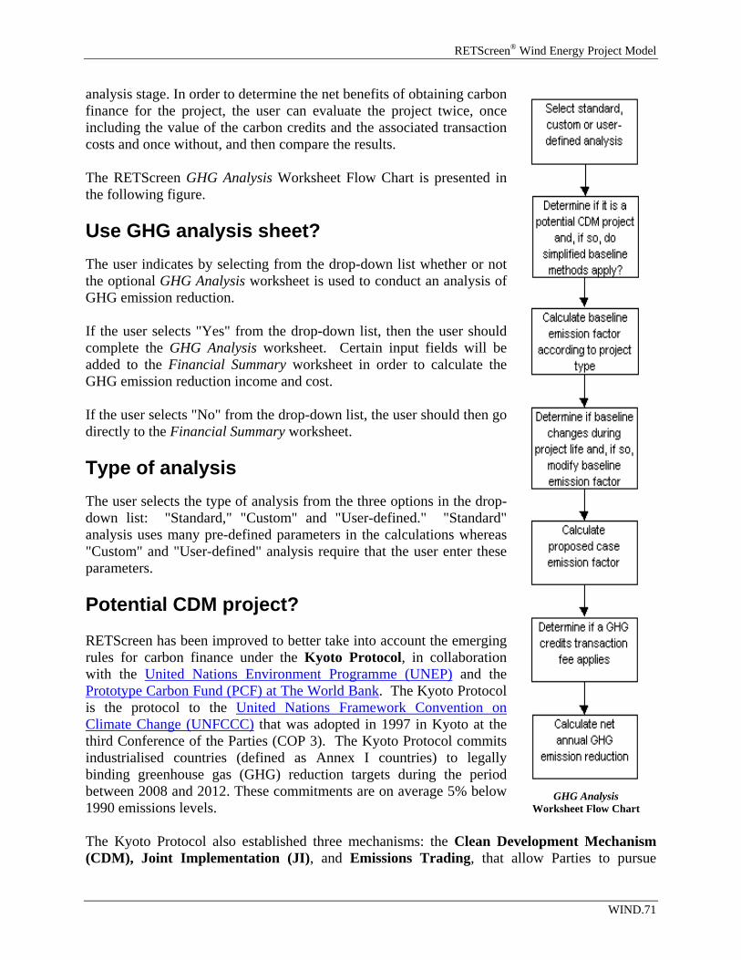
RETScreen® Wind Energy Project Model
analysis stage. In order to determine the net benefits of obtaining carbon finance for the project, the user can evaluate the project twice, once including the value of the carbon credits and the associated transaction costs and once without, and then compare the results.
Wo
The RETScreen GHG Analysis Worksheet Flow Chart is presented in the following figure. Use GHG analysis sheet? The user indicates by selecting from the drop-down list whether or not the optional GHG Analysis worksheet is used to conduct an analysis of GHG emission reduction. If the user selects "Yes" from the drop-down list, then the user should complete the GHG Analysis worksheet. Certain input fields will be added to the Financial Summary worksheet in order to calculate the GHG emission reduction income and cost. If the user selects "No" from the drop-down list, the user should then go directly to the Financial Summary worksheet. Type of analysis The user selects the type of analysis from the three options in the drop-down list: "Standard," "Custom" and "User-defined." "Standard" analysis uses many pre-defined parameters in the calculations whereas "Custom" and "User-defined" analysis require that the user enter these parameters. Potential CDM project? RETScreen has been improved to better take into account the emerging rules for carbon finance under the Kyoto Protocol, in collaboration with the United Nations Environment Programme (UNEP) and the Prototype Carbon Fund (PCF) at The World Bank. The Kyoto Protocol is the protocol to the United Nations Framework Convention on Climate Change (UNFCCC) that was adopted in 1997 in Kyoto at the third Conference of the Parties (COP 3). The Kyoto Protocol commits industrialised countries (defined as Annex I countries) to legally binding greenhouse gas (GHG) reduction targets during the period between 2008 and 2012. These commitments are on average 5% below 1990 emissions levels. The Kyoto Protocol also established three mechanisms: the Clean Develop(CDM), Joint Implementation (JI), and Emissions Trading, that allow
GHG Analysis rksheet Flow Chart
ment Mechanism Parties to pursue
WIND.71
RETScreen® Software Online User Manual
opportunities to cut emissions, or enhance carbon sinks, abroad. The cost of curbing emissions varies considerably from region to region and therefore makes economic sense to cut emissions, where it is cheapest to do so, given that the impact on the atmosphere is the same. The user indicates by selecting from the drop-down list whether or not the project is to be evaluated as a potential CDM project. The user should select "Yes" if the project is located in a developing country and it has good potential to meet the requirements for CDM projects. These requirements are described in brief below and covered in detail at the UNFCCC's CDM Website. The user should select "No" for any other domestic or international GHG reduction projects, including ones that might qualify for Joint Implementation. JI requirements are also described in brief below. If the user selects "Yes" from the drop-down list, RETScreen automatically assesses, by checking values calculated on other RETScreen worksheets, whether or not the project can be considered as a small-scale CDM project (i.e. the capacity of a renewable energy system does not exceed 15 MW or the aggregate energy savings by an energy efficiency improvement project does not exceed the equivalent of 15 GWh per year). If the project fits within the criteria for small-scale CDM projects, then the user may be able to take advantage of the simplified baseline methods and other rules and procedures for small-scale CDM projects. The basic concept of the Clean Development Mechanism is that industrialised countries (or companies) invest in GHG emission-reduction projects in developing countries and gain credits from these projects that they can then apply to their own GHG reduction commitments as agreed to under the Kyoto Protocol. Article 12 of the Kyoto Protocol defines the goals of the CDM as:
• to assist developing countries in achieving sustainable development, and in contributing to the ultimate objective of the Convention; and
• to assist industrialised countries in meeting their quantified emission reduction commitments.
The Kyoto Protocol also proscribes that emissions reductions will only be certified if:
• the CDM project has the approval of the host country; • the project produces real, measurable and long-term GHG benefits; and • the reductions in emissions are additional to any that would occur in the absence of the
certified project activity. Under the Kyoto Protocol an Executive Board (EB) has been established to oversee and monitor the CDM. The Executive Board is responsible for accrediting Designated Operational Entities (DOE) that validate CDM projects and verify and certify emissions reductions. Credits generated and certified from CDM projects are known as "Certified Emissions Reductions," or CERs. A CER is equal to one metric tonne of carbon dioxide (CO2) equivalent and must be certified by a Designated Operational Entity.
WIND.72

RETScreen® Wind Energy Project Model
In November 2001, at COP 7 in Marrakech, Morocco, the parties reached an agreement on the legal text needed to implement the Kyoto Protocol. A key outcome of Marrakech was agreement on the basic rules and regulations governing the CDM. These rules are covered in a section of the Marrakech Accord known as "Modalities and Procedures for a Clean Development Mechanism." Specific issues agreed to in Marrakech include the baseline approaches that will be permitted for CDM projects, the procedures for approving baseline methodologies, and the format of the Project Design Document (PDD). Marrakech also allowed for simplified procedures for small-scale projects and identified the types of projects that could be considered small scale. All CDM projects must be "additional to any that would occur in the absence of the proposed project activity" in order to be eligible for credits. This qualification is called "additionality." All CDM projects, therefore, require the estimation or measurement of "baseline" emissions - those that would have occurred without the project - and actual emissions that occur after a project has been implemented. Guidelines are available at the UNFCCC's CDM Website on how to demonstrate additionality. A baseline approach is the basis for defining a baseline methodology. The Conference of the Parties have agreed to the following three approaches for CDM project activities.
1. Existing actual or historical emissions, as applicable.
2. Emissions from a technology that represents an economically attractive course of action, taking into account barriers to investment.
3. The average emissions of similar project activities undertaken in the previous five years,
in similar social, economic, environmental and technological circumstances, and whose performance is among the top 20 per cent of their category.
The RETScreen GHG Analysis worksheet can be used for each of these approaches. Note that although the Executive Board has approved these three baseline approaches, they are simply guidelines. In order to register a CDM project the baseline must be developed using an approved methodology. A baseline methodology is an application of one of the allowable baseline approaches, as defined to an individual project activity, reflecting aspects such as sector and region. Baseline methodologies for CDM projects must be approved by the Executive Board. If project proponents wish to use a new methodology they may submit it for approval. Details of approved methodologies are provided at the UNFCCC's CDM Website. Joint Implementation projects, on the other hand, occur in Annex 1 countries, that is, countries that have agreed to emissions targets under the Kyoto Protocol. Like the CDM, the basic concept of JI is that industrialised countries (or companies) invest in GHG emission-reduction projects in other Annex 1 countries where reductions are cheaper than in their own country and gain credits from these projects that can then applied to their own GHG reduction commitments as agreed to under Kyoto. In practice, Joint Implementation projects are more likely to take place
WIND.73
RETScreen® Software Online User Manual
in Economies-In-Transition or EITs, where there tends to be more scope for cutting emissions at lower costs. Joint Implementation projects must have the approval of all Parties involved, and must lead to emission reductions or removals that are additional to any that would have occurred without the project. An ERU is an Emission Reduction Unit generated from a JI project. An ERU is equal to one metric tonne of carbon dioxide (CO2) equivalent. Projects starting from the year 2000 that meet the above rules may be listed as Joint Implementation projects. However, ERUs may only be issued after 2008.1 Use simplified baseline methods RETScreen automatically assesses, by checking values calculated on other RETScreen worksheets, whether or not the project can be considered as a small-scale CDM project (i.e. the capacity of a renewable energy system does not exceed 15 MW or the aggregate energy savings by an energy efficiency improvement project does not exceed the equivalent of 15 GWh per year). Note that this option will automatically be hidden in RETScreen for non-CDM projects, or for potential CDM projects that exceed the small-scale CDM project size limits. Simplified rules and procedures are available for small-scale CDM projects if it can be demonstrated that one of the barriers identified by the UNFCCC has been overcome in order to implement the project. These simplifications will allow the use of standardized baselines, streamlined monitoring procedures, a simpler Project Design Document, and reduced registration fees - all of which reduce transaction costs so that small-scale projects can offer CERs at more competitive prices. The user should select "Yes" from the drop-down list to indicate that the simplified methods will be used for developing the baseline for the potential small-scale CDM project. The RETScreen GHG Analysis worksheet can be used to calculate the baseline for a small-scale CDM project directly in conjunction with Appendix B of the document "Simplified modalities and procedures for small-scale CDM project activities," which is available at the UNFCCC's CDM Website. This appendix contains indicative simplified baseline and monitoring methodologies for selected small-scale CDM project activity categories, including recommendations for determining the project boundary, leakage, baseline and monitoring. Note that small-scale CDM projects should not be debundled components of larger project activities, as described in Appendix C. In accordance with the simplified modalities and procedures for small-scale CDM project activities, a simplified baseline and monitoring methodology listed in the appendix may be used for a small-scale CDM project activity if project participants are able to demonstrate to a designated operational entity that the project activity would otherwise not be implemented due to the existence of one or more barrier(s) listed on the next page. 1 Portions of this text were adapted from the UNFCCC's document, Guide to the Climate Convention and its Kyoto Protocol, available at UNFCCC's Website.
WIND.74
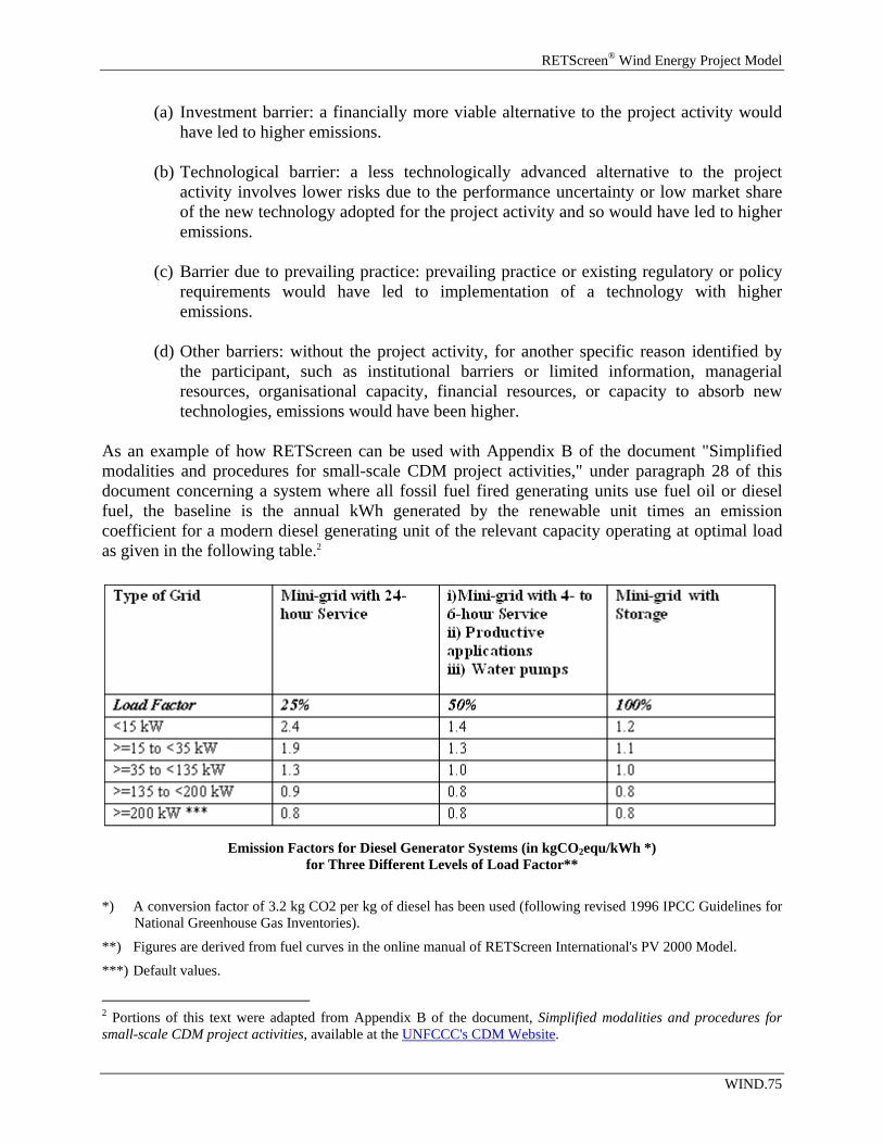
RETScreen® Wind Energy Project Model
(a) Investment barrier: a financially more viable alternative to the project activity would have led to higher emissions.
(b) Technological barrier: a less technologically advanced alternative to the project
activity involves lower risks due to the performance uncertainty or low market share of the new technology adopted for the project activity and so would have led to higher emissions.
(c) Barrier due to prevailing practice: prevailing practice or existing regulatory or policy
requirements would have led to implementation of a technology with higher emissions.
(d) Other barriers: without the project activity, for another specific reason identified by
the participant, such as institutional barriers or limited information, managerial resources, organisational capacity, financial resources, or capacity to absorb new technologies, emissions would have been higher.
As an example of how RETScreen can be used with Appendix B of the document "Simplified modalities and procedures for small-scale CDM project activities," under paragraph 28 of this document concerning a system where all fossil fuel fired generating units use fuel oil or diesel fuel, the baseline is the annual kWh generated by the renewable unit times an emission coefficient for a modern diesel generating unit of the relevant capacity operating at optimal load as given in the following table.2
Emission Factors for Diesel Generator Systems (in kgCO2equ/kWh *)
for Three Different Levels of Load Factor** *) A conversion factor of 3.2 kg CO2 per kg of diesel has been used (following revised 1996 IPCC Guidelines for
National Greenhouse Gas Inventories).
**) Figures are derived from fuel curves in the online manual of RETScreen International's PV 2000 Model.
***) Default values.
2 Portions of this text were adapted from Appendix B of the document, Simplified modalities and procedures for small-scale CDM project activities, available at the UNFCCC's CDM Website.
WIND.75
RETScreen® Software Online User Manual
In this example, the user would select "User-defined" type of analysis at the top of the RETScreen GHG Analysis Worksheet and enter "diesel mini-grid" as the electricity system under the Base Case Electricity System (Baseline) section, and then enter the appropriate GHG coefficient as selected from the table above. Note that the UNFCCC used RETScreen to help calculate the emission factors at different load levels for the table provided above. Background Information Project name The user-defined project name is entered for reference purposes only in the Energy Model worksheet, and it is copied automatically to the GHG Analysis worksheet. Project location The user-defined project location is entered for reference purposes only in the Energy Model worksheet, and it is copied automatically to the GHG Analysis worksheet. Project capacity The project capacity is calculated in the Energy Model worksheet and it is copied automatically to the GHG Analysis worksheet. Grid type The grid type is selected in the Energy Model worksheet, and it is copied automatically to the GHG Analysis worksheet. Global Warming Potential of GHG The model indicates the global warming potential of methane (CH4) and nitrous oxide (N2O). If the user selects the "Custom" type of analysis, different values from the default values provided may be entered by the user. Researchers have assigned Global Warming Potentials (GWPs) to greenhouse gases to allow for comparisons of their relative heat-trapping effect. The higher the global warming potential of a gas the greater the contribution to the greenhouse effect. For example nitrous oxide is 310 times more effective than carbon dioxide at trapping heat in the atmosphere. GWPs of gases are defined as a unit multiple of that given to carbon dioxide (CO2), which is assigned a reference value of 1 (i.e., the GWP of CO2 is 1 and the GWP of N2O is 310). The default values are those defined by the Revised Intergovernmental Panel on Climate Change (IPCC) Guidelines for Greenhouse Gas Inventories, 1996.
WIND.76
RETScreen® Wind Energy Project Model
Base Case Electricity System (Baseline) To perform the RETScreen GHG emission reduction analysis for the project, the user needs to define the baseline (also called base case or reference case) electricity system. For example, in North America when preparing a GHG emission reduction analysis for a wind energy project where central-grid electricity is used, it is often reasonable to assume that a combined-cycle natural gas power plant is the proxy plant. In this case the user needs only to select "Natural gas" as the fuel type with a 100% fuel mix and use the default "T & D losses" of 8%. For the case of an isolated-grid or an off-grid application, a diesel genset would likely be the "proxy" power plant with "Diesel (#2 oil)" chosen as the fuel type. It is also possible to define the grid and the mix of the different power plants with their respective fuels, fuel mix and different T & D losses (e.g. distributed generators such as photovoltaics will have lower T & D losses). This information is usually available through the local electric utility, the utility regulator and/or through government. For example, the United States Environmental Protection Agency (US-EPA) provides "The Emissions & Generation Resource Integrated Database" called E-GRID. This is a database featuring environmental characteristics of electric power generation in the US, including fuel mix. This database is available free of charge at the E-GRID Website. To illustrate this alternative analysis method, for a grid-connected project based in Nova Scotia, Canada, the provincial government might determine the baseline to be the weighted average of the current generation mix. This can be calculated by simply entering the current fuel mix into the grid along with the appropriate emissions coefficient. For this example and with information provided by Natural Resources Canada, the user would select the following fuel types and associated fuel mix: coal with 78% of the fuel mix, large hydro with 9%, #6 oil with 5%, natural gas with 5% and biomass with 3% of the fuel mix and T & D losses of 8% for all fuel types. Note that this methodology can be used for small-scale CDM renewable energy projects that are connected to a grid that includes generating units other than diesel or fuel oil. Some users may prefer to perform a much more detailed analysis of the GHG reduction potential of the project (e.g. an economist working for a public utility commission). The model allows for a more detailed analysis regarding T & D losses and using the "Custom" option under the "Type of analysis" drop-down list, the user can prepare an even more detailed analysis regarding emission factors, etc. If the user has access to dispatch information from the local utility, the Base Case Electricity System table can be used to model the marginal fuel use on the grid, which may more accurately represent the fuels and the emissions that are being displaced by the proposed project. For example, if dispatch information shows that the fuel used on the margin is natural gas 85% of the time and fuel oil 15% of the time, the user would enter these details into the base case table along with the corresponding GHG coefficients. The resulting baseline is often referred to as the "operating margin."
WIND.77
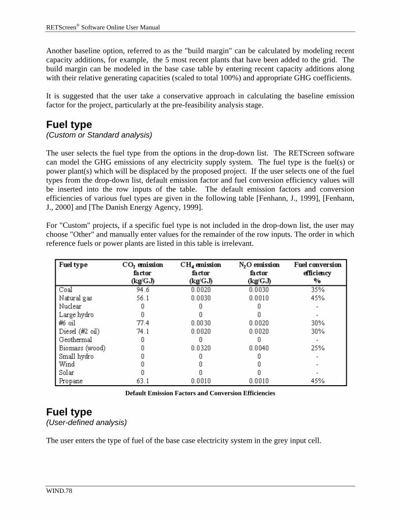
RETScreen® Software Online User Manual
Another baseline option, referred to as the "build margin" can be calculated by modeling recent capacity additions, for example, the 5 most recent plants that have been added to the grid. The build margin can be modeled in the base case table by entering recent capacity additions along with their relative generating capacities (scaled to total 100%) and appropriate GHG coefficients. It is suggested that the user take a conservative approach in calculating the baseline emission factor for the project, particularly at the pre-feasibility analysis stage. Fuel type (Custom or Standard analysis) The user selects the fuel type from the options in the drop-down list. The RETScreen software can model the GHG emissions of any electricity supply system. The fuel type is the fuel(s) or power plant(s) which will be displaced by the proposed project. If the user selects one of the fuel types from the drop-down list, default emission factor and fuel conversion efficiency values will be inserted into the row inputs of the table. The default emission factors and conversion efficiencies of various fuel types are given in the following table [Fenhann, J., 1999], [Fenhann, J., 2000] and [The Danish Energy Agency, 1999]. For "Custom" projects, if a specific fuel type is not included in the drop-down list, the user may choose "Other" and manually enter values for the remainder of the row inputs. The order in which reference fuels or power plants are listed in this table is irrelevant.
Default Emission Factors and Conversion Efficiencies
Fuel type (User-defined analysis) The user enters the type of fuel of the base case electricity system in the grey input cell.
WIND.78
RETScreen® Wind Energy Project Model
Fuel mix The user enters the fuel mix (%) of the base case electricity system for each fuel type. Units are given as percentages of total electricity supplied. Note that the user should verify that the sum of all fuel types listed in the fuel mix column equals 100%. CO2, CH4 and N2O emission factors (Custom analysis) The user enters the CO2, CH4 and N2O emission factors for the different fuel types. They represent the mass of greenhouse gas emitted per unit of energy. Emission factors will vary for different types and qualities of fuels, and for different types and sizes of power plants. For grid-connected projects, the user should enter factors representative of large generating plants. On the electricity mix row at the bottom of the table, the model calculates the equivalent emission factors for the global electricity mix and per unit of electricity delivered. The electricity mix factors thus account for a weighted average of the fuel conversion efficiencies and T & D losses of the different fuel types. For each fuel type selected, units are given in kilograms of gas emitted per gigajoule of heat energy generated (kg/GJ). For the global electricity mix shown on the bottom row of the table, units are given in kilograms of gas emitted per gigajoule of end-use electricity delivered. For more information on determining GHG emission factors, see the revised IPCC Guidelines for National Greenhouse Gas Inventories. CO2 emission factors for many fuels are included on page 1.13 of the IPCC Reference Manual. CH4 and N2O emission factors for a number of fuels are included on pages 1.35 and 1.36 of the IPCC Reference Manual. In addition, refer to the National Communications at the UNFCCC Website to see if more relevant emission factors are available for the country being considered.
CO2, CH4 and N2O emission factors (Standard analysis) The model provides the CO2, CH4 and N2O emission factors which represent the mass of greenhouse gas emitted per unit of energy. Emission factors will vary for different types and qualities of fuels, and for different types and sizes of power plants. The default factors provided are those which are representative of large power plants that feed a central electricity grid. On the electricity mix row at the bottom of the table, the model calculates the equivalent emission factors for the total electricity mix and per unit of electricity delivered. The electricity mix factors thus account for a weighted average of the fuel conversion efficiencies and T & D losses of the different fuel types. For each fuel type selected, units are given in kilograms of gas emitted per gigajoule of heat energy generated (kg/GJ). For the total electricity mix shown on the bottom row of the table, units are given in kilograms of gas emitted per gigajoule of end-use electricity delivered.
WIND.79
RETScreen® Software Online User Manual
For more information on determining GHG emission factors, see the revised IPCC Guidelines for National Greenhouse Gas Inventories. CO2 emission factors for many fuels are included on page 1.13 of the IPCC Reference Manual. CH4 and N2O emission factors for a number of fuels are included on pages 1.35 and 1.36 of the IPCC Reference Manual. In addition, refer to the National Communications at the UNFCCC Website to see if more relevant emission factors are available for the country being considered. The default values provided by the model are given in the Default Emission Factors and Conversion Efficiencies table. Fuel conversion efficiency (Custom analysis) The user enters the fuel conversion efficiency for the selected fuel type. The fuel conversion efficiency is the efficiency of energy conversion from primary heat potential to actual power plant output. This value is used to calculate, for each fuel type, the aggregate GHG emission factor and therefore is only relevant for fuel types which actually produce greenhouse gases (i.e. with non-zero CO2, CH4 and N2O emission factors). For example, a typical coal-fired power plant could have a fuel conversion efficiency of 35%, which indicates that 35% of the heat content of the coal is transformed into electricity fed to the grid. Units are given as a percentage of primary heat potential (gigajoules of heat) to actual power plant output (gigajoules of electricity). Fuel types which emit no GHGs (e.g. solar) have a default value of 100%. Fuel conversion efficiency (Standard analysis) The model provides the fuel conversion efficiency for the selected fuel type. The fuel conversion efficiency is the efficiency of energy conversion from primary heat potential to actual power plant output. This value is used to calculate, for each fuel type, the aggregate GHG emission factor and therefore is only relevant for fuel types which actually produce greenhouse gases (i.e. with non-zero CO2, CH4 and N2O emission factors). For example, a typical coal-fired power plant could have a fuel conversion efficiency of 35%, which indicates that 35% of the heat content of the coal is transformed into electricity fed to the grid. Units are given as a percentage of primary heat potential (gigajoules of heat) to actual power plant output (gigajoules of electricity). Fuel types which emit no GHGs (e.g. solar) have a default value of 100%. The default values provided by the model are given in the Default Emission Factors and Conversion Efficiencies table.
WIND.80
RETScreen® Wind Energy Project Model
Transmission and distribution losses The user enters the transmission and distribution (T & D) losses (%) of the base case electricity system, which includes all energy losses between the power plant and the end-user. This value will vary based on the voltage of transport lines, the distance from the site of energy production to the point of use, peak energy demands, ambient temperature and electricity theft. In addition, T & D system type (e.g. AC vs. DC) and quality may also influence losses. The model calculates the weighted average of the T & D losses of the global electricity mix on the bottom row of the table. Units are given as a percentage of all electricity losses to electricity generated. As a first estimate, it is reasonable to assume T & D losses of 8 to 10% in modern grids in industrialised countries and 10 to 20% in grids located in developing countries.
GHG emission factor (Custom or Standard analysis) The model calculates the GHG emission factor for each reference fuel type. Values are calculated based on the individual emission factors, the fuel conversion efficiency and the T & D losses. The weighted GHG emission factor for the total electricity mix is calculated on the bottom row of the table. Units are given in tonnes equivalent of CO2 emissions per megawatt-hour of end-use electricity delivered (tCO2 / MWh). GHG emission factor (User-defined analysis) The user enters the GHG emission factor for the base case electricity system specified. Units switch: The user can choose to express the emission factor in kgCO2 / kWh or in tCO2 / MWh (which are equivalent). Base case GHG emission factor The model calculates the GHG emission factor for the electricity system specified. The value is calculated based on the GHG emission factor and the T & D losses entered by the user. Units are given in tonnes equivalent of CO2 emissions per megawatt-hour of end-use electricity delivered (tCO2 / MWh).
Does baseline change during project life? The user indicates by selecting from the drop-down menu whether or not the baseline changes during the project life. The project baseline might not stay constant throughout the life of the
WIND.81
RETScreen® Software Online User Manual
project, due to factors such as changes in regulations in the electricity sectors, the planned addition of new generation units on the grid (eg. large-scale hydroelectric project), or decommissioning of existing units. The model allows for one change in the baseline during the project life that the user enters as a percentage increase or decrease in the initial baseline. The baseline emissions will thus be scaled accordingly for the year in which the change occurs as well as each year following the change. Change in GHG emission factor The user enters the percentage by which baseline emissions will increase (positive percentage) or decrease (negative percentage) because of the change in the baseline. For example, if a new hydro plant already under construction will decrease emissions by 10% in year 5, then the user enters negative 10%. The model will then reduce baseline emissions by 10% for year 5 and all subsequent years.
Year of change The user enters the year in which the change in the baseline occurs. For example, if a new hydro plant is scheduled to be added to the electricty grid during the fifth year after this proposed project begins, the user enters 5. GHG emission factor year x and beyond The model calculates the GHG emission factor for the years following the change in baseline. Values are calculated by applying the specified change in emission factor to the weighted GHG emission factor of the electricity mix. Units are given in tonnes equivalent of CO2 emissions per megawatt-hour of end-use electricity delivered (tCO2 / MWh).
Reason/event for baseline change The user enters the reason for the baseline change, i.e. the event that triggers the change in the baseline. This information is given for reference purposes only. For example, if the addition of a new hydro plant is the reason for the change in the baseline, the user would enter something like "Addition of new hydro plant already planned."
Proposed Case Electricity System (Wind Energy Project) The proposed case electricity system, or mitigation system, is the proposed project. The GHG emissions for the proposed project are assumed to be equal to zero.
WIND.82
RETScreen® Wind Energy Project Model
The proposed case system is normally referred to as the mitigation option in standard economic analysis.
Fuel type The fuel type of the proposed project is assumed to be an emission free source.
Fuel mix The fuel mix of the proposed project is set to 100%. CO2, CH4 and N2O emission factors (Custom analysis) The user enters the CO2, CH4 and N2O emission factors corresponding to the fuel type, i.e. the proposed system. Units are given in kilograms of gas emitted per gigajoule of energy produced (kg/GJ). CO2, CH4 and N2O emission factors (Standard analysis) The model provides the CO2, CH4 and N2O emission factors corresponding to the fuel type, i.e. the proposed system. These values are assumed to be zero in all cases. Units are given in kilograms of gas emitted per gigajoule of energy produced (kg/GJ). Fuel conversion efficiency If the user selects the "Standard" type of analysis, the fuel conversion efficiency is set to 100% for the proposed project. For "Custom" type of analysis, the user enters the fuel conversion efficiency. This value is used in conjunction with the CO2, CH4 and N2O emission factors and the transmission and distribution losses to calculate the aggregate GHG emission factor for the proposed project. Transmission and distribution losses The user enters the transmission and distribution (T & D) losses (%) of the proposed project, which includes all energy losses between the point at which the power plant is connected to the grid and the end-user. This value will vary based on the voltage of transport lines, the distance from the site of energy production to the point of use, peak energy demands, ambient temperature and electricity theft. In addition, T & D system type (e.g. AC vs. DC) and quality may also influence losses.
WIND.83
RETScreen® Software Online User Manual
Units are given as a percentage of all electricity losses to electricity generated. As a first estimate, it is reasonable to assume T & D losses of 8 to 10% in modern grids in industrialised countries and 10 to 20% in grids located in developing countries. GHG emission factor The model calculates the GHG emission factor for the proposed project. Values are calculated based on the individual emission factors and the fuel conversion efficiency. Units are given in tonnes equivalent of CO2 emissions per megawatt-hour of end-use electricity delivered (tCO2 / MWh). Proposed case GHG emission factor The user enters the GHG emission factor for the proposed project. Units switch: The user can choose to express the emission factor in kgCO2 / kWh or in tCO2 / MWh (which are equivalent). GHG Emission Reduction Summary Based on the GHG emission data entered, the model calculates the annual reduction in GHG emissions when the base case system is displaced with the proposed case system. If the baseline changes during the project life, then the model calculates the annual GHG reduction for both periods of the base case, that is, for the years before the change in baseline and for the years following the change in baseline. Years of occurrence If the user has entered that the project baseline does change, the model indicates the year numbers for the first period GHG emission factors and for the second period GHG emission factors.
Base case GHG emission factor The model transfers the base case GHG emission factor calculated in the base case electricity system (baseline) section. This value represents the amount of GHG emitted per unit of end-use electricity delivered for the base case system. Units switch: The user can choose to express the emission factor in kgCO2 / kWh or in tCO2 / MWh (which are equivalent).
WIND.84
RETScreen® Wind Energy Project Model
Proposed case GHG emission factor The model transfers the proposed case GHG emission factor calculated (or entered by the user) in the Proposed Case Electricity System section. Units switch: The user can choose to express the emission factor in kgCO2 / kWh or in tCO2 / MWh (which are equivalent).
End-use annual energy delivered The model calculates the end-use annual energy delivered by the proposed project which is the amount of energy delivered to the electricity grid (or load for off-grid systems), as calculated in the Energy Model worksheet, minus the T & D losses for the grid vis-à-vis the proposed project. Units are given in megawatt-hours of end-use electricity delivered (MWh). Gross annual GHG emission reduction The model calculates the gross annual reduction in GHG emissions estimated to occur if the proposed project is implemented. The calculation is based on emission factors of both the base case and the proposed case system and on the end-use electricity delivered by the proposed project on an annual basis. Units are given in equivalent tonnes of CO2 emissions per year (tCO2/yr). GHG credits transaction fee The user enters the percentage of credits that will have to be paid annually as a transaction fee. In order to obtain credits for a GHG project, a portion of the credits might have to be subtracted as a transaction fee, to be paid each year to the crediting agency (e.g. the UNFCCC) and/or the host country. For CDM projects 2% of the CERs generated by each project will be paid into an Adaptation fund to help particularly vulnerable developing countries adapt to climate change. Note that projects in least developed countries are exempt from this part of the levy in order to promote the equitable distribution of projects. The CDM Executive Board, as well as a number of host countries, also require that they receive a percentage of the credits to help cover their administrative costs (e.g. for project approval etc.). The user might wish to check the UNFCCC's CDM Website and with the host country's Designated National Authority to find out if they require a percentage of credits to be paid.3 The model then reduces the annual GHG credits by this percentage before it calculates the total GHG credits and the value of these credits.
3 A list of Designated National Authorities, is available at the UNFCCC's CDM Website.
WIND.85
RETScreen® Software Online User Manual
Net annual GHG emission reduction The model calculates the net annual reduction in GHG emissions estimated to occur if the proposed project is implemented. The calculation is based on the gross annual GHG emission reduction and the GHG credits transaction fee. Units are given in equivalent tonnes of CO2 emissions per year (tCO2/yr). Note: At this point, the user should complete the Financial Summary worksheet.
WIND.86
RETScreen® Wind Energy Project Model
Sensitivity and Risk Analysis As part of the RETScreen Clean Energy Project Analysis Software, a Sensitivity and Risk Analysis worksheet is provided to help the user estimate the sensitivity of important financial indicators in relation to key technical and financial parameters. This standard sensitivity and risk analysis worksheet contains two main sections: Sensitivity Analysis and Risk Analysis. Each section provides information on the relationship between the key parameters and the important financial indicators, showing the parameters which have the greatest impact on the financial indicators. The Sensitivity Analysis section is intended for general use, while the Risk Analysis section, which performs a Monte Carlo simulation, is intended for users with knowledge of statistics. Both types of analysis are optional. Inputs entered in this worksheet will not affect results in other worksheets. Use sensitivity analysis sheet? The user indicates, by selecting from the drop-down list, whether or not the optional Sensitivity and Risk Analysis worksheet is used to conduct a sensitivity analysis of the important financial indicators. If the user selects "Yes" from the drop-down list, the sensitivity analysis section will open and the user should complete the top part of the worksheet. Perform risk analysis too? The user indicates, by selecting from the drop-down list, whether or not the optional risk analysis section is used to conduct a risk analysis of the important financial indicators, in addition to the sensitivity analysis. In the risk analysis section, the impact of each input parameter on a financial indicator is obtained by applying a standardised multiple linear regression on the financial indicator. If the user selects "Yes" from the drop-down list, then the risk analysis section will open and the user should complete the lower-half of the worksheet. The analysis will be performed on the financial indicator selected by the user in the "Perform analysis on" input cell at the top-right.
Project name The user-defined project name is entered for reference purposes only in the Energy Model worksheet, and it is copied automatically to the Sensitivity worksheet. Project location The user-defined project location is entered for reference purposes only in the Energy Model worksheet, and it is copied automatically to the Sensitivity worksheet.
WIND.87
RETScreen® Software Online User Manual
Perform analysis on The user selects, from three options in the drop-down list, the financial indicator to be used for both the sensitivity and risk analyses. Modifying the selection in this cell will change the results in the worksheet. Sensitivity range The user enters the sensitivity range (%), which defines the maximum percentage variation that will be applied to all the key parameters in the sensitivity analysis results tables. Each parameter is varied by the following fraction of the sensitivity range: -1, -1/2, 0, 1/2, 1. This value is used in the sensitivity analysis section only. The sensitivity range entered by the user must be a percentage value between 0 and 50%. Threshold The user enters the threshold value for the financial indicator selected. The threshold is the value under which (for the "After tax IRR and ROI" and "Net Present Value - NPV") or over which (for "Year-to-positive cash flow") the user considers that the proposed project is not financially viable. Results which indicate an unviable project, as defined by the user threshold, will appear as orange cells in the sensitivity analysis results tables. This value is used in the sensitivity analysis section only.
Click here to Calculate Sensitivity Analysis The "Click here to Calculate Sensitivity Analysis" button updates the sensitivity analysis calculations using the input parameters specified by the user (i.e. "Perform analysis on" and "Sensitivity range" input cells). The sensitivity analysis tables are updated each time the user clicks on this button. The sensitivity analysis calculations can take some time to run depending of the Excel version (e.g. approximately 2 to 40 sec. with Excel 2003 and 2002; 20 to 120 sec. with Excel 2000 and 97). When the sensitivity analysis is updated, the button disappears. If the user makes any changes to the input parameters, or navigates through any of the other worksheets, the button will reappear. The user will then have to click on the button to update the sensitivity analysis calculations so that the results reflect the changes. Sensitivity Analysis for... This section presents the results of the sensitivity analysis. Each table shows what happens to the selected financial indicator (e.g. After-tax IRR and ROI) when two key parameters (e.g. Initial costs and Avoided cost of energy) are varied by the indicated percentages. Parameters are varied using the following fraction of the sensitivity range: -1, -1/2, 0, 1/2, 1. Original values (which
WIND.88
RETScreen® Wind Energy Project Model
appear in the Financial Summary worksheet) are in bold in these sensitivity analysis results tables. Results which indicate an unviable project, as defined by the user threshold, will appear as orange cells in these sensitivity analysis results tables. All parameter values used for the calculations are taken from the Financial Summary worksheet and all the sensitivity variations are evaluated at the level of that worksheet. This is a partial limitation of this sensitivity analysis worksheet since some parameter values are calculated from inputs in other worksheets, but those inputs are not changed. However, for most cases, this limitation is without consequence. If required, the user can use the blank worksheets (Sheet1, etc.) to perform a more detailed analysis. Risk Analysis for... This section allows the user to perform a Risk Analysis by specifying the uncertainty associated with a number of key input parameters and to evaluate the impact of this uncertainty on after-tax IRR and ROI, year-to-positive cash flow or net present value (NPV). The risk analysis is performed using a Monte Carlo simulation that includes 500 possible combinations of input variables resulting in 500 values of after-tax IRR and ROI, year-to-positive cash flow or net present value (NPV). The risk analysis allows the user to assess if the variability of the financial indicator is acceptable, or not, by looking at the distribution of the possible outcomes. An unacceptable variability will be an indication of a need to put more effort into reducing the uncertainty associated with the input parameters that were identified as having the greatest impact on the financial indicator. Avoided cost of energy The avoided cost of energy is automatically transferred from the Financial Summary worksheet to the Sensitivity worksheet. The user enters the avoided cost of energy range. The range is a percentage corresponding to the uncertainty associated with the estimated avoided cost of energy value. The higher the percentage, the greater the uncertainty. The range specified by the user must be between 0 and 50%. The range determines the limits of the interval of possible values that the avoided cost of energy could take. For example, a range of 10% for an avoided cost of energy of 0.09 $/kWh means that the avoided cost of energy could take any value between 0.081$/kWh and 0.099 $/kWh. Since 0.09 $/kWh is the estimated value, the risk analysis will consider this value as being the most probable and the minimum and maximum values as being the least probable, based on a normal distribution. If the avoided cost of energy is known exactly by the user (no uncertainty), the user should enter a range of 0%.
WIND.89
RETScreen® Software Online User Manual
Renewable energy delivered The RE delivered is transferred automatically from the Financial Summary worksheet to the Sensitivity worksheet. The user enters the RE delivered range. The range is a percentage corresponding to the uncertainty associated with the estimated RE delivered value. The higher the percentage, the greater the uncertainty. The range specified by the user must be between 0 and 50%. The range determines the limits of the interval of possible values that the RE delivered could take. For example, a range of 10% for a RE delivered of 40,000 MWh means that the RE delivered could take any value between 36,000 MWh and 44,000 MWh. Since 40,000 MWh is the estimated value, the risk analysis will consider this value as being the most probable and the minimum and maximum values as being the least probable, based on a normal distribution. If the RE delivered is known exactly by the user (no uncertainty), the user should enter a range of 0%.
Initial costs The total initial cost is transferred automatically from the Financial Summary worksheet to the Sensitivity worksheet. The user enters the initial costs range. The range is a percentage corresponding to the uncertainty associated with the estimated initial costs value. The higher the percentage, the greater the uncertainty. The range specified by the user must be between 0 and 50%. The range determines the limits of the interval of possible values that the initial costs could take. For example, a range of 10% for initial costs of $30,000,000 means that the initial costs could take any value between $27,000,000 and $33,000,000. Since $30,000,000 is the estimated value, the risk analysis will consider this value as being the most probable and the minimum and maximum values as being the least probable, based on a normal distribution. If the initial costs are known exactly by the user (no uncertainty), the user should enter a range of 0%. Annual costs The annual cost is transferred automatically from the Financial Summary worksheet to the Sensitivity worksheet, but does not include debt payments. The user enters the annual cost range. The range is a percentage corresponding to the uncertainty associated with the estimated annual costs value. The higher the percentage, the greater the uncertainty. The range specified by the user must be between 0 and 50%. The range determines the limits of the interval of possible values that the annual costs could take.
WIND.90
RETScreen® Wind Energy Project Model
For example, a range of 10% for an annual cost of $80,000 means that the annual cost could take any value between $72,000 and $88,000. Since $80,000 is the estimated value, the risk analysis will consider this value as being the most probable and the minimum and maximum values as being the least probable, based on a normal distribution. If the annual costs are known exactly by the user (no uncertainty), the user should enter a range of 0%.
Debt ratio The debt ratio is automatically transferred from the Financial Summary worksheet to the Sensitivity worksheet. The user enters the debt ratio range. The range is a percentage corresponding to the uncertainty associated with the estimated debt ratio value. The higher the percentage, the greater the uncertainty. The range specified by the user must be a percentage value between 0% and the lowest percentage such that the debt ratio will always fall between 0 and 100%. The range determines the limits of the interval of possible values that the debt ratio could take. For example, a range of 10% for a debt ratio of 70% means that the debt ratio could take any value between 63 and 77%. Since 70% is the estimated value, the risk analysis will consider this value as being the most probable and the minimum and maximum values as being the least probable, based on a normal distribution. If the debt ratio is known exactly by the user (no uncertainty), the user should enter a range of 0%. Debt interest rate The debt interest rate is automatically transferred from the Financial Summary worksheet to the Sensitivity worksheet. The user enters the debt interest rate range. The range is a percentage corresponding to the uncertainty associated with the estimated debt interest rate value. The higher the percentage, the greater the uncertainty. The range specified by the user must be between 0 and 50%. The range determines the limits of the interval of possible values that the debt interest rate could take. For example, a range of 10% for a debt interest rate of 20% means that the debt interest rate could take any value between 18 and 22%. Since 20% is the estimated value, the risk analysis will consider this value as being the most probable and the minimum and maximum values as being the least probable, based on a normal distribution. If the debt interest rate is known exactly by the user (no uncertainty), the user should enter a range of 0%.
WIND.91
RETScreen® Software Online User Manual
Debt term The debt term is automatically transferred from the Financial Summary worksheet to the Sensitivity worksheet. The user enters the debt term range. The range is a percentage corresponding to the uncertainty associated with the estimated debt term value. The higher the percentage, the greater the uncertainty. The range specified by the user must be a percentage value between 0% and the lowest percentage such that the debt term will always fall between 1 year and the project life. The range determines the limits of the interval of possible values that the debt term could take. For example, a range of 10% for a debt term of 20 years means that the debt term could take any value between 18 and 22 years. Since 20 years is the estimated value, the risk analysis will consider this value as being the most probable and the minimum and maximum values as being the least probable, based on a normal distribution. If the debt term is known exactly by the user (no uncertainty), the user should enter a range of 0%.
GHG emission reduction credit The GHG emission reduction credit is automatically transferred from the Financial Summary worksheet to the Sensitivity worksheet. The user enters the GHG emission reduction credit range. The range is a percentage corresponding to the uncertainty associated with the estimated GHG emission reduction credit value. The higher the percentage, the greater the uncertainty. The range specified by the user must be a percentage value between 0 and 50%. The range determines the limits of the interval of possible values that the GHG emission reduction credit could take. For example, a range of 10% for a GHG emission reduction credit of $5/tCO2 means that the GHG emission reduction credit could take any value between $4.5/tCO2 and $5.5/tCO2. Since $5/tCO2 is the estimated value, the risk analysis will consider this value as being the most probable and the minimum and maximum values as being the least probable, based on a normal distribution. If the GHG emission reduction credit is known exactly by the user (no uncertainty), the user should enter a range of 0%.
RE production credit The RE production credit is automatically transferred from the Financial Summary worksheet to the Sensitivity worksheet. The user enters the RE production credit range. The range is a percentage corresponding to the uncertainty associated with the estimated RE production credit value. The higher the percentage, the greater the uncertainty. The range specified by the user must be a percentage value between 0
WIND.92
RETScreen® Wind Energy Project Model
and 50%. The range determines the limits of the interval of possible values that the RE production credit could take. For example, a range of 10% for a RE production credit of $0.05/kWh means that the RE production credit could take any value between $0.045/kWh and $0.055/kWh. Since $0.05/kWh is the estimated value, the risk analysis will consider this value as being the most probable and the minimum and maximum values as being the least probable, based on a normal distribution. If the RE production credit is known exactly by the user (no uncertainty), the user should enter a range of 0%.
Click here to Calculate Risk Analysis The "Click here to Calculate Risk Analysis" button updates the risk analysis calculations using the input parameter ranges specified by the user. Clicking on this button starts a Monte Carlo simulation that uses 500 possible combinations of input variables resulting in 500 values of the selected financial indicator. The impact graph, the median, the minimum and maximum confidence levels, and the distribution graph are calculated using these results and updated each time the user clicks on the button "Click here to Calculate Risk Analysis." Since the time required by the software to run the Monte Carlo simulation is relatively significant (e.g. approximately 1 to 4 min. with Excel 2003 and 2002; 2 to 20 min. with Excel 2000 and 97), it is recommended that the user click on this button only after having input all the range values. When the risk analysis is updated, the button disappears. If the user makes any changes to the input range values, or navigates through any of the other worksheets, the button will reappear. The user will then have to click on the button to update the risk analysis calculations so that the results reflect the changes. Impact graph The impact graph shows the relative contribution of the uncertainty in each key parameter to the variability of the financial indicator. The X axis at the bottom of the graph does not have any units, but rather presents a relative indication of the strength of the contribution of each parameter. The longer the horizontal bar, for a given input parameter, the greater is the impact of the input parameter on the variability of the financial indicator. The input parameters are automatically sorted by their impact on the financial indicator. The input parameter at the top (Y axis) contributes the most to the variability of the financial indicator while the input parameter at the bottom contributes the least. This "tornedo graph" will help the user determine which input parameters should be considered for a more detailed analysis, if that is required. The direction of the horizontal bar (positive or negative) provides an indication of the relationship between the input parameter and the financial indicator. There is a positive relationship between
WIND.93
RETScreen® Software Online User Manual
an input parameter and the financial indicator when an increase in the value of that parameter results in an increase in the value of the financial indicator. For example, there is usually a negative relationship between initial costs and the net present value (NPV), since decreasing the initial costs will increase the NPV. In some cases, there is insufficient data to properly plot the graph. For example, when the year-to-positive cash flow is immediate, the result is not a numerical value, and therefore these values cannot be plotted.
Median The model calculates the median of the financial indicator. The median of the financial indicator is the 50th percentile of the 500 values generated by the Monte Carlo simulation. The median will normally be close to the financial indicator value calculated in the Financial Summary worksheet.
Level of risk The user selects from the drop-down list the acceptable level of risk for the financial indicator under consideration. The options are: 5%, 10%, 15%, 20% and 25%. The level of risk input is used to establish a confidence interval (defined by maximum and minimum limits) within which the financial indicator is expected to fall. The level of risk represents the probability that the financial indicator will fall outside this confidence interval. The limits of the confidence interval are automatically calculated based on the median and the level of risk, and are shown as "Minimum within level of confidence" and "Maximum within level of confidence." It is suggested that the user select a level of risk of 5 or 10%, which are typical values for standard risk analysis. Minimum within level of confidence The model calculates the "Minimum within level of confidence," which is the lower limit of the confidence interval within which the financial indicator likely falls. It is the percentile of the distribution of the financial indicator corresponding to half the level of risk defined by the user. For example, for a "Minimum within level of confidence" value of 15% IRR, a level of risk of 10% means that 5% (half the level of risk) of the possible IRR values are lower than 15%. Maximum within level of confidence The model calculates the "Maximum within level of confidence," which is the upper limit of the confidence interval within which the financial indicator likely falls. It is the percentile of the distribution of the financial indicator corresponding to 100% minus half the level of risk. For example, for a "Maximum within level of confidence" value of 25% IRR, a level of risk of 10% means that 95% of the possible IRR values are lower than 25%.
WIND.94
RETScreen® Wind Energy Project Model
Distribution graph This histogram provides a distribution of the possible values for the financial indicator resulting from the Monte Carlo simulation. The height of each bar represents the frequency (%) of values that fall in the range defined by the width of each bar. The value corresponding to the middle of each range is plotted on the X axis. Looking at the distribution of financial indicator, the user is able to rapidly assess its' variability. In some cases, there is insufficient data to properly plot the graph. For example, when the year-to-positive cash flow is immediate, the result is not a numerical value, and therefore these values cannot be plotted. Bar graph The bar graph summarises the maximum and minimum financial indicator values that can be expected according to the level of risk defined by the user.
WIND.95

RETScreen® Software Online User Manual
Product Data Some of the product data requirements for the model are provided in the RETScreen Online Product Database. To access the product database the user may refer to "Data & Help Access." The product database provides information on the equipment associated with the project. From the online product database dialogue box the user may obtain product specification and performance data, as well as company contact information. From the dialogue box the user selects the Wind Turbine Rated Power Range (kW), followed by the Region, Supplier, Model and Details. The data can be pasted from the dialogue box to the spreadsheets by clicking on the "Paste Data" button. Only data that are in bold are pasted to the spreadsheets; all other data are provided for reference purposes only. Data entered using the product database may be overwritten; i.e. the user may prefer to use other data and can manually enter values into the spreadsheets. "Other information" such as product weight and/or dimensions, is provided to help the user prepare the study. The product database contains a link to the Websites of some product suppliers. In the case where the Website link cannot be activated the user should try using another browser or can contact the supplier by other means (email, fax, etc.). Note: To see all the suppliers listed in the product database and their contact information, the user can choose "Any" from the "Wind Turbine Rated Power Range (kW)" input cell. The product database is distributed for informational purposes only and does not necessarily reflect the views of the Government of Canada nor constitute an endorsement of any commercial product or person. Neither Canada nor its ministers, officers, employees or agents make any warranty in respect to this database or assumes any liability arising out of this database. Product manufacturers interested in having their products listed in the product database can reach RETScreen® International at: RETScreen® International CANMET Energy Technology Centre - Varennes Natural Resources Canada 1615 Lionel-Boulet, P.O. Box 4800 Varennes, Quebec, CANADA J3X 1S6 Tel: +1-450-652-4621 Fax: +1-450-652-5177 E-mail: [email protected]
WIND.96

RETScreen® Wind Energy Project Model
Weather Data This database includes some of the weather data required in the model. To access the weather database the user may refer to "Data & Help Access." While running the software the user may obtain weather data from ground monitoring stations, from NASA's satellite data, and/or from other data sources such as the Solar and Wind Energy Resource Assessment (SWERA). Ground monitoring stations data is obtained by making a selection for a specific location from the online weather database dialogue box. Data sets from other sources are obtained via the "Visit Other Data Sites" button in the dialogue box. Ground Monitoring Stations Data From the dialogue box, the user selects a region, then a country, then a sub-region (provinces in Canada, states in the United States and N/A in the rest of the countries), and finally a weather station location. The weather station usually corresponds to the name of a city/town within the selected country. From the dialogue box the data can be pasted to the spreadsheets by clicking on the "Paste Data" button. Only data that are in bold are pasted to the spreadsheets; all other data are provided for reference purposes only. Data entered using the online weather database may be overwritten; i.e. the user may prefer to use other data and can manually enter values into the spreadsheets. As an alternative the user can use resource maps or the NASA satellite data, particularly for the case when the project location is not close to the given weather station location.
NASA Global Satellite Data A link to the NASA Surface meteorology and Solar Energy Data Set Website is provided in the online weather database dialogue box ("Visit Other Data Sites"). The user is able to select the data required for the model by clicking on a region on the world map illustrated on the NASA Website. The location is narrowed down to a "cell" within a specified latitude and longitude. The user may simply copy and paste this data to the RETScreen spreadsheets or manually enter these values. NASA and CETC - Varennes are co-operating to facilitate the use of NASA's global satellite solar data with RETScreen and to develop a new global weather database (see Surface meteorology and Solar Energy Data Set for the tool). This work is sponsored as part of NASA's Earth Science Enterprise Program and is being carried out at the NASA Langley Research Center and at CETC-Varennes. This collaboration provides RETScreen users access (free-of-charge) to satellite data (e.g. the amount of solar energy striking the surface of the earth, global temperatures and wind speeds), simply by clicking on links in either the RETScreen software or the NASA Website. These data had previously only been available from a limited number of ground monitoring stations and are critical for assessing the amount of energy a project is expected to produce. The use of these data results in substantial cost savings for users and increased market opportunities for industry while allowing governments and industry to evaluate regional energy resource potential.
WIND.97

RETScreen® Software Online User Manual
Cost Data Typical cost data required to prepare RETScreen studies are provided in the RETScreen Online Cost Database and in the Online Manual. This database is built into the "right-hand column" of the Cost Analysis worksheet. Data are provided for Canadian costs with 2000 as a baseline year. The user also has the ability to create a custom cost database. The user selects the reference (from the Cost Analysis worksheet) that will be used as a guideline for the estimation of costs associated with the implementation of the project. This feature allows the user to change the "Quantity Range" and the "Unit Cost Range" columns. The options from the drop down list are: "Canada - 2000," "None," "Second currency" and a selection of 8 user-defined options ("Enter new 1," "Enter new 2," etc.). If the user selects "Canada - 2000" the range of values reported in the "Quantity Range" and "Unit Cost Range" columns are for a 2000 baseline year, for projects in Canada and in Canadian dollars. Selecting "None" hides the information presented in the "Quantity Range" and "Unit Cost Range" columns. The user may choose this option, for example, to minimise the amount of information printed in the final report. If the user selects "Second currency" two additional input cells appear in the next row: "Second currency" and "Rate: 1st currency / 2nd currency." In addition, the "Quantity Range" and "Unit Cost Range" columns change to "% Foreign" and "Foreign Amount," respectively. This option allows the user to assign a portion of a project cost item in a second currency, to account for those costs that must be paid for in a currency other than the currency in which the project costs are reported. Note that this selection is for reference purposes only, and does not affect the calculations made in other worksheets. If "Enter new 1" (or any of the other 8 selections) is selected, the user may manually enter quantity and cost information that is specific to the region in which the project is located and/or for a different cost base year. This selection thus allows the user to customise the information in the "Quantity Range" and "Unit Cost Range" columns. The user can also overwrite "Enter new 1" to enter a specific name (e.g. Japan - 2001) for a new set of unit cost and quantity ranges. The user may also evaluate a single project using different quantity and cost ranges; selecting a new range reference ("Enter new 1" to "Enter new 8") enables the user to keep track of different cost scenarios. Hence the user may retain a record of up to 8 different quantity and cost ranges that can be used in future RETScreen analyses and thus create a localised cost database.
WIND.98

RETScreen® Wind Energy Project Model
Training and Support The user can obtain current information on RETScreen Training & Support at the following Website address: www.retscreen.net/e/training. .
WIND.99

RETScreen® Software Online User Manual
Terms of Use
Disclaimer and Indemnification RETScreen® International is provided on an "as is" basis. Natural Resources Canada nor does its minister, officers, employees or agents make any representations or warranties, either expressed or implied, arising by law or otherwise, including but not limited to, implied warranties of merchantability or fitness for a particular purpose, or that the use of the software will not infringe any intellectual property rights of third parties. In no event will Natural Resources Canada nor its minister, officers, employees or agents have any obligations or liability arising from tort, or for loss of revenue or profit, or for indirect, special, incidental or consequential damages as a result of your use of the software. In consideration of the right to load, execute and use RETScreen® International, the recipient (Licensee) shall indemnify and save harmless Natural Resources Canada (Licensor), and its employees and agents, from and against, and shall be responsible for all claims, demands, losses, costs, including solicitor and client costs, damages, actions suits or proceedings, arising out of, related to, or occasioned by any use of RETScreen International by the Licensee. The Licensor shall have the right to defend any such action or proceeding with counsel of its own selection.
Copyright and Trademark The RETScreen® International Clean Energy Project Analysis Software and the accompanying manual and databases are copyright of the Minister of Natural Resources Canada (1997 - 2004). Duplication in any manner is forbidden without prior written permission, which may be obtained by contacting: RETScreen® International CANMET Energy Technology Centre - Varennes Natural Resources Canada 1615 Lionel-Boulet, P.O. Box 4800 Varennes, Quebec, CANADA J3X 1S6 Tel: +1-450-652-4621 Fax: +1-450-652-5177 E-mail: [email protected] © Minister of Natural Resources Canada 1997 - 2004. RETSCREEN® is a registered trademark of the Minister of Natural Resources Canada.
WIND.100

RETScreen® Wind Energy Project Model
License Agreement The use of RETScreen® International is subject to the terms detailed in the RETScreen Software License Agreement, which is available at the following Website address: www.retscreen.net/license.html/. The user is encouraged to properly register at the RETScreen Website so that the Centre may periodically inform the user of product upgrades and be able to report on the global use of RETScreen.
WIND.101

RETScreen® Software Online User Manual
Bibliography Brothers, C., Wind Generation Systems for Remote Communities - Market Assessment and Guidelines for Wind Turbines Selection, Canadian Electrical Association Project #9123 G 880, June 1993. Canadian Wind Energy Association (CanWEA), Wind Energy Basic Information, Backgrounder published with support from CANMET, 1996. Conover, K., Wind Energy Financial Due Diligence, R. Lynette & Associates, Seminar on Opportunities for Finance and Investment in Wind Energy, November, 1994. The Danish Energy Agency, Engerstatistics 1995, 1999. Elliot, D. et al., Wind Energy Resource Atlas of the United States, SERI, October 1986. Fenhann, J., "Personal Communication," January 2000. Fenhann, J., Projections of Emissions of Greenhouse Gases, Ozone precursors and Sulphur Dioxide from Danish Sources until 2010, The Danish Energy Agency, December 1999. Gipe, P., Wind Energy Comes of Age, John Wiley and Sons, 1995. Johansson et al., Renewable Energy - Sources for Fuels and Electricity, Island Press, 1993. Le Gouriérès, D., Wind Power Plants: Theory and Design, Pergamon Press, 1982. Leng, G., RETScreen International: A Decision-Support and Capacity-Building Tool for Assessing Potential Renewable Energy Projects, UNEP Industry & Environment, 3rd Quarter, 2000. Leng, G., Dignard-Bailey, L., Bragagnolo, J., Tamizhmani, G. and Usher, E., Overview of the Worldwide Photovoltaic Industry, report # 96-41-A1 (TR), CANMET Energy Diversification Research Laboratory, Natural Resources Canada, Varennes, June 1996. Leng, G., J. Martin, Distributed Photovoltaic Demand-Side Generation: An Economic Evaluation For Electric Utilities, IEEE First World Conference On Photovoltaic Energy Conversion, December 1994. Leng, G., Distributed Photovoltaic Demand-Side Generation: An Economic Evaluation For Electric Utilities - Master Degree Thesis, University of Massachusetts Lowell, November 1993. Lynette, R. and Ass., Technical and Economic Potential for Wind Energy Development in Ontario, prepared for Independent Power Producers' Society of Ontario, April 1992.
WIND.102

RETScreen® Wind Energy Project Model
Martinot, E. and McDoom, O., Promoting Energy Efficiency and Renewable Energy: GEF Climate Change Projects and Impacts, October 1999 Pre-Publication Draft, Global Environment Facility, 1999. Rangi, R., Templin, J., M. Carpentier and Argue, D., Canadian Wind Energy Technical and Market Potential, EAETB, Energy, Mines and Resources Canada, October 1992. Reid, R., Application de l'éolien aux réseaux non-reliés, Hydro-Québec, Congrès de l'ACFAS, Montréal, 1996. Sandor, R., Walsh, M. and Leblanc, A., Creating a Market for Carbon Emissions: Gas Industry Opportunities, published in Natural Gas, June 1999. Sigma Engineering Ltd, Energy Overview Study of Remote Communities in Canada, prepared for the Remote Community Demonstration Program, Energy Mines and Resources Canada, March 1985. SunMedia GmbH, Wind Turbine Market: Types, Technical Characteristics, Prices, 1999. United Nations Framework Convention on Climate Change (UNFCCC) Clean Development Mechanism (CDM) Executive Board, Annex B - Indicative simplified baseline and monitoring methodologies for selected small-scale CDM project activity categories, December 2002. Vesterdal, J., The Potential of Wind Farms, ELSAM, 1992. WECTEC, Évaluation du potentiel éolien du Québec, Report prepared for the Ministère des Ressources Naturelles du Québec, February 1996. Wind Power Monthly, Operating Wind Power Capacity, July 2000. Winkra-Recom, Wind Turbine Market - Types, Technical Characteristics, Prices, 1995/96. Zond, Wind Power Economics, presented at the seminar Opportunities for Finance and Investment in Wind Energy, November 1994.
WIND.103
RETScreen® Software Online User Manual
Website Addresses Canada's Clean Development Mechanism (CDM): http://www.dfait-maeci.gc.ca/cdm-ji/cleandev-en.asp Canada's Joint Implementation (JI): http://www.dfait-maeci.gc.ca/cdm-ji/joint-en.asp Canadian Wind Atlas: http://www.cmc.ec.gc.ca/rpn/modcom/eole/CanadianAtlas.html Environment Canada - Canadian Weather Energy and Engineering Data Sets: http://www.climate.weatheroffice.ec.gc.ca European Wind Resources: http://www.windatlas.dk/Europe/About.html Intergovernmental Panel on Climate Change (IPCC) Guidelines for National Greenhouse Gas Inventories: http://www.ipcc-nggip.iges.or.jp/public/gl/invs1.htm IPCC Reference Manual page 1.13: http://www.ipcc-nggip.iges.or.jp/public/gl/guidelin/ch1ref1.pdf IPCC Reference Manual pages 1.35 and 1.36: http://www.ipcc-nggip.iges.or.jp/public/gl/guidelin/ch1ref2.pdf NASA Surface meteorology and Solar Energy Data Set: http://eosweb.larc.nasa.gov/sse/RETScreen/ National Climatic Data Center: http://www.ncdc.noaa.gov National Wind Technology Center (NWTC): http://www.nrel.gov/wind/wind_map.html Prototype Carbon Fund (PCF) at World Bank: http://prototypecarbonfund.org/ RETScreen: www.retscreen.net RETScreen Development Team: www.retscreen.net/e/partners/ RETScreen Software License Agreement: www.retscreen.net/license.html/ RETScreen Training & Support: www.retscreen.net/e/training/ Solar and Wind Energy Resource Assessment: http://swera.unep.net/ United Nations Environment Programme (UNEP): http://www.unepie.org/energy/ United Nations Framework Convention on Climate Change (UNFCCC): http://unfccc.int/ UNFCCC Clean Development Mechanism (CDM): http://cdm.unfccc.int/ U.S. Environmental Protection Agency - Emissions and Generation Resource Integrated Database: http://www.epa.gov/cleanenergy/egrid/index.html
WIND.104

RETScreen® Wind Energy Project Model
WIND.105
RETScreen® Software Online User Manual
Index
A
After-tax .......................................................65, 69, 88 After-tax IRR and ROI.............................................88 Airfoil soiling and/or icing losses ............................17 Annual average temperature.....................................13 Annual average wind speed......................................11 Annual costs .................................................48, 69, 90 Annual Costs (Credits) .............................................47 Annual Energy Balance............................................52 Annual Energy Production .......................................18 Annual Life Cycle Savings ......................................67 Annual Savings or Income .......................................63 Annual wind power density......................................11 Array losses..............................................................17 Average atmospheric pressure .................................12 Avoided cost of capacity ....................................57, 64 Avoided cost of energy ..........................54, 64, 88, 89 Avoided cost of excess energy ...........................57, 64
B
Background Information ....................................70, 76 Balance of Plant .......................................................42 Bar graph..................................................................95 Base Case Electricity System (Baseline)............76, 77 Base case GHG emission factor .........................81, 84 Benefit-Cost (B-C) ratio...........................................67 Bibliography...........................................................102 Blank Worksheets (3)...........................................9, 69 Brief Description and Model Flow Chart...................4
C
Calculate energy production cost? ...........................67 Calculate GHG reduction cost?................................68 Capacity savings/income..........................................64 Cell Colour Coding ....................................................5 Change in GHG emission factor ..............................82 Civil design ..............................................................38 Click here to Calculate Risk Analysis......................93 Click here to Calculate Sensitivity Analysis ............88 Commissioning ........................................................46 Community benefits .................................................49 Construction supervision..........................................39 Control and O&M building(s)..................................45 Copyright and Trademark ......................................100 Cost Analysis ... 6, 9, 25, 26, 49, 52, 59, 61, 62, 64, 98 Cost Data..................................................................98 Cost references ...............................................6, 26, 27 Cumulative ...............................................................69
Cumulative Cash Flows Graph................................ 69 Currency ........................................................ 6, 26, 28 Currency Options....................................................... 6
D
Data & Help Access ................................ 5, 10, 96, 97 Debt interest rate................................................ 59, 91 Debt payments ................................................... 63, 68 Debt payments - debt term....................................... 63 Debt ratio ........................................................... 58, 91 Debt service coverage.............................................. 68 Debt term........................................................... 59, 92 Depreciation method................................................ 60 Depreciation period ................................................. 61 Depreciation rate...................................................... 61 Depreciation tax basis.............................................. 61 Detailed cost estimate .............................................. 31 Development31, 33, 35, 46, 49, 57, 62, 70, 71, 72, 73,
102, 103, 104 Disclaimer and Indemnification ............................ 100 Discount rate............................................................ 58 Distribution graph.................................................... 95 Does baseline change during project life? ............... 81
E
Effective income tax rate ......................................... 59 Electrical design ...................................................... 38 End of project life ........................................ 51, 60, 64 End of project life - Cost/Credit .............................. 64 End-use annual energy delivered............................. 85 Energy cost escalation rate ...................................... 58 Energy curve data .............................................. 22, 23 Energy curve data source................................... 22, 23 Energy Equipment ................................................... 40 Energy Model 9, 10, 14, 15, 21, 22, 23, 24, 52, 53, 76,
85, 87 Energy production cost ............................................ 67 Energy savings/income............................................ 64 Engineering.................................. 31, 37, 62, 103, 104 Environmental assessment....................................... 30 Equipment Data ................................. 9, 14, 15, 18, 21 Excess RE available........................................... 53, 64
F
Feasibility Study................................................ 29, 62 Financial Feasibility .......................................... 52, 65 Financial Parameters.......................................... 52, 54 Financial Summary....9, 19, 20, 52, 53, 54, 61, 69, 70,
71, 86, 89, 90, 91, 92, 94
WIND.106
RETScreen® Wind Energy Project Model
Firm RE capacity..........................................53, 57, 64 Foreign Amount ...........................................27, 28, 98 Fuel conversion efficiency .................................80, 83
G
General and administrative.......................................50 GHG baseline study and monitoring plan ................31 GHG credit escalation rate ...........................56, 57, 64 GHG credits transaction fee .........................68, 85, 86 GHG emission factor year x and beyond .................82 GHG emission reduction cost ..................................68 GHG emission reduction credit..56, 57, 64, 67, 68, 92 GHG Emission Reduction Summary .................70, 84 GHG monitoring and verification ......................47, 49 GHG reduction credit duration...........................53, 56 GHG reduction income - duration............................64 GHG validation and registration ........................33, 35 Global Warming Potential of GHG..........................76 Greenhouse Gas Emission Reduction Analysis .........9 Grid type ......................................................13, 53, 76 Gross annual GHG emission reduction ....................85 Gross energy production ....................................17, 18 Ground Monitoring Stations Data ............................97
H
Height of wind measurement ...................................12 Height of wind power density ............................11, 15 Hub height..........................................................15, 21
I
Impact graph ............................................................93 Incentives/Grants......................................................63 Inflation....................................................................58 Initial costs .........................................................88, 90 Initial Costs (Credits) ...............................................28 Insurance premium...................................................48 Interest during construction......................................47
L
Land lease ................................................................47 Land rights ...............................................................34 Land survey..............................................................35 Legal and accounting ...............................................36 Level of risk .............................................................94 License Agreement.........................................101, 104 Loss carryforward?...................................................60 Losses coefficient.....................................................19
M
Maximum within level of confidence...................... 94 Mechanical design ................................................... 38 Median..................................................................... 94 Minimum within level of confidence....................... 94 Miscellaneous ........................................ 17, 18, 46, 63 Miscellaneous losses.......................................... 17, 18 Model Flow Chart...................................................... 4
N
NASA Global Satellite Data.................................... 97 Nearest location for weather data ............................ 11 Net annual GHG emission reduction ....................... 86 Net GHG emission reduction - credit duration ........ 53 Net GHG emission reduction - project life .............. 54 Net GHG emission reduction - yr x+1 and beyond
(2nd period) ........................................................ 54 Net GHG emission reduction [ yr 1 to x (1st period)]
............................................................................ 53 Net Present Value - NPV................................... 67, 88 Number of turbines.................................................. 14
O
O&M ................................... 34, 42, 45, 46, 47, 49, 63 Other downtime losses............................................. 17
P
Parts and labour ....................................................... 48 Peak load ..................................................... 14, 15, 53 Perform analysis on ........................................... 87, 88 Perform risk analysis too? ....................................... 87 Periodic Costs (Credits)..................................... 50, 64 Permits and approvals.............................................. 34 Potential CDM project? ........................................... 71 Power curve data ..................................................... 23 PPA negotiation....................................................... 33 Preliminary design................................................... 30 Pressure adjustment coefficient ............................... 18 Pre-tax ............................................................... 65, 69 Printing a File ............................................................ 8 Product Data .....5, 7, 10, 21, 22, 23, 25, 40, 41, 42, 96 Project Costs and Savings.................................. 52, 61 Project debt.............................................................. 68 Project equity........................................................... 68 Project financing...................................................... 36 Project life ............................................................... 58 Project location...................................... 10, 52, 76, 87 Project name .......................................... 10, 52, 76, 87 Property taxes .......................................................... 48
WIND.107
RETScreen® Software Online User Manual
Proposed Case Electricity System (Wind Energy Project) ................................................................82
Proposed case GHG emission factor ..................84, 85
R
Rate 1st currency / 2nd currency .....................27, 28, 98
RE credit escalation rate.....................................56, 64 RE production credit ..................55, 56, 64, 67, 92, 93 RE production credit duration ............................56, 64 RE production credit income - duration ...................64 Reason/event for baseline change ............................82 Renewable energy collected.....................................19 Report preparation....................................................32 Road construction.....................................................43 Rotor diameter..........................................................21
S
Saving a File...............................................................7 Second currency .................................6, 26, 27, 28, 98 Sensitivity and Risk Analysis...............................9, 87 Sensitivity range.......................................................88 Shape factor..............................................................22 Simple Payback........................................................66 Site Conditions .........................................................10 Site investigation......................................................29 Spare parts................................................................41 Specific yield............................................................19 Substation.................................................................44 Suggested wind energy absorption rate....................16 Swept area ................................................................21 System Characteristics .............................................13
T
Tax holiday available? .............................................61 Tax holiday duration ................................................61 Temperature adjustment coefficient.........................18 Tenders and contracting ...........................................39 Terms of Use..........................................................100 Threshold .................................................................88 Training......................................................46, 99, 104 Training and Support................................................99 Transmission line ...............................................44, 48
Transmission line maintenance................................ 48 Type of analysis................................................. 71, 77 Type of project ........................................................ 25
U
Unadjusted energy production................................. 18 Unit Options .............................................................. 7 Units ..7, 10, 14, 18, 20, 49, 79, 80, 81, 82, 83, 84, 85,
86 Use GHG analysis sheet?......................................... 71 Use sensitivity analysis sheet?................................. 87
W
Weather Data ............................... 5, 10, 11, 12, 13, 97 Website Addresses................................................. 104 Wind data source ..................................................... 10 Wind energy absorption rate.................................... 16 Wind Energy Project Model ................................ 9, 16 Wind penetration level............................................. 15 Wind plant capacity ............................... 14, 15, 18, 19 Wind plant capacity factor....................................... 19 Wind power density at hub height ........................... 15 Wind resource assessment ....................................... 30 Wind shear exponent ............................................... 12 Wind speed ...................................... 10, 11, 12, 15, 23 Wind speed at 10 m ................................................. 12 Wind speed at hub height ........................................ 15 Wind Turbine Characteristics .................................. 21 Wind turbine manufacturer...................................... 22 Wind turbine model ................................................. 22 Wind Turbine Power and Energy Curves ................ 24 Wind Turbine Production Data................................ 23 Wind turbine rated power .................................. 14, 21 Wind turbine(s)...................................... 37, 40, 42, 43 Wind turbine(s) erection.......................................... 43 Wind turbine(s) foundation(s) ................................. 42 Wind turbine(s) micro-siting ................................... 37
Y
Year of change......................................................... 82 Yearly Cash Flows............................................. 52, 69 Year-to-positive cash flow................................. 66, 88
WIND.108

RETScreen® Wind Energy Project Model
NOTES:
WIND.109