Page 1
REVENUE MAXIMIZATION USING PRODUCT BUNDLING
by
Mihai Banciu
B.B.A., Romanian-American University, 1999
M.B.A., James Madison University, 2002
Submitted to the Graduate Faculty of
The Joseph M. Katz Graduate School of Business in partial fulfillment
of the requirements for the degree of
Doctor of Philosophy
University of Pittsburgh
2009
Page 2
ii
UNIVERSITY OF PITTSBURGH
THE JOSEPH M. KATZ GRADUATE SCHOOL OF BUSINESS
This dissertation was presented
by
Mihai Banciu
It was defended on
July 29, 2009
and approved by
Dissertation Chair: Prakash Mirchandani, Professor, Katz Graduate School of Business
Esther Gal-Or, Professor, Katz Graduate School of Business
Brady Hunsaker, Google Inc.
Jerrold May, Professor, Katz Graduate School of Business
R. Venkatesh, Associate Professor, Katz Graduate School of Business
Page 3
iii
Copyright © by Mihai Banciu
2009
Page 4
iv
Product bundling is a business strategy that packages (either physically or logically), prices and
sells groups of two or more distinct products or services as a single economic entity. This
practice exploits variations in the reservation prices and the valuations of a bundle vis-à-vis its
constituents. Bundling is an effective instrument for price discrimination, and presents
opportunities for enhancing revenue without increasing resource availability. However, optimal
bundling strategies are generally difficult to derive due to constraints on resource availability,
product valuation and pricing relationships, the consumer purchase process, and the rapid growth
of the number of possible alternatives.
This dissertation investigates two different situations—vertically differentiated versus
independently valued products—and develops two different approaches for revenue
maximization opportunities using product bundling, when resource availability is limited. For
the vertically differentiated market with two products, such as the TV market with prime time
and non-prime time advertising, we derive optimal policies that dictate how the seller (that is, the
broadcaster) can manage their limited advertising time inventories. We find that, unlike other
markets, the revenue maximizing strategy may be to offer only the bundle, only the components,
or various combinations of the bundle and the components. The optimality of these strategies
critically depends on the availability of the two advertising time resources. We also show how
the network should focus its programming quality improvement efforts, and investigate how the
REVENUE MAXIMIZATION USING PRODUCT BUNDLING
Mihai Banciu, PhD
University of Pittsburgh, 2009
Page 5
v
“value of bundling,” defined as the network’s and the advertisers’ benefit from bundling,
changes as the resource availabilities change. We then propose and study a bundling model for
the duopolistic situation, and extend the results from the monopolistic to the duopolistic case.
For the independently valued products, we develop stochastic mathematical programming
models for pricing bundles of n components. Specializing this model for two components in a
deterministic setting, we derive closed-form optimal product pricing policies when the demand
functions are linear. Using the intuition garnered from these analytical results, we then
investigate two procedures for solving large-scale problems: a greedy heuristic, and a
decomposition method. We show the effectiveness of both methods through computational
experiments.
Page 6
vi
TABLE OF CONTENTS
ACKNOWLEDGMENTS ........................................................................................................ XII
1.0 INTRODUCTION ........................................................................................................ 1
1.1 REVENUE MANAGEMENT AND PRODUCT BUNDLING ........................ 3
1.2 OBJECTIVES OF THIS WORK ....................................................................... 6
1.3 OVERVIEW OF CHAPTERS ......................................................................... 10
2.0 REVENUE MANAGEMENT AND PRODUCT BUNDLING .............................. 12
2.1 BUNDLING STRATEGIES ............................................................................. 16
2.2 FORECASTING ................................................................................................ 19
2.3 THE MEDIA ADVERTISING MARKET ...................................................... 21
2.4 BUNDLING IN COMPETITIVE ENVIRONMENTS .................................. 22
2.5 SUMMARY ........................................................................................................ 23
3.0 MIXED BUNDLING PRICING STRATEGIES FOR THE TV ADVERTISING
MARKET..................................................................................................................................... 25
3.1 INTRODUCTION ............................................................................................. 25
3.2 THE GENERAL MIXED BUNDLING MODEL ........................................... 31
3.3 REVENUE MAXIMIZING STRATEGIES WHEN CAPACITY IS
BINDING ............................................................................................................................. 39
3.3.1 Characterization of the different strategies ................................................ 42
Page 7
vii
3.3.2 Optimal product prices and shadow prices ................................................. 46
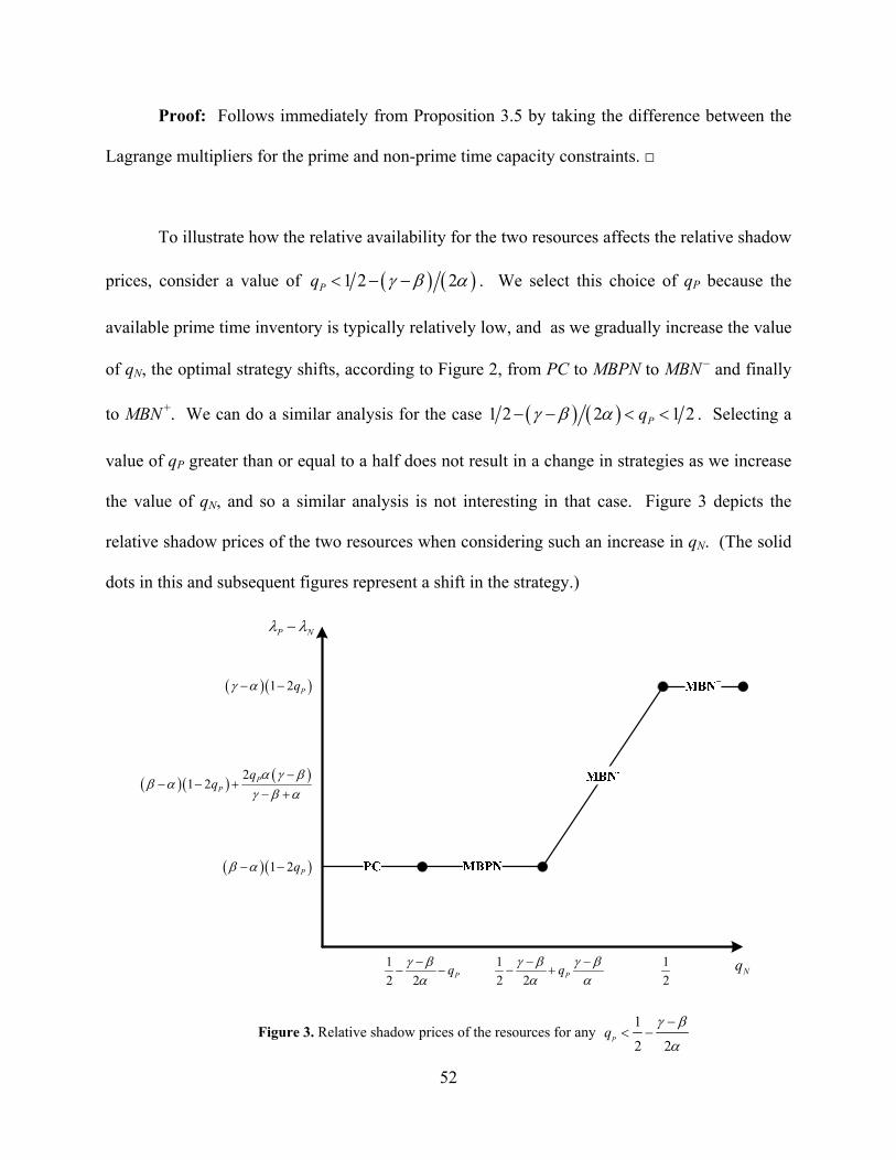
3.3.3 Relative shadow prices .................................................................................. 51
3.3.4 Incentives for improving the programming quality ................................... 54
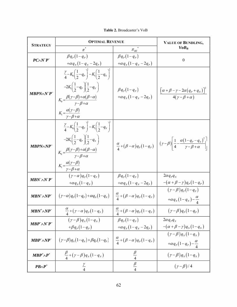
3.4 VALUE OF BUNDLING .................................................................................. 59
3.4.1 Broadcaster’s Value of Bundling ................................................................. 59
3.4.2 Advertisers’ Value of Bundling .................................................................... 65
3.4.3 Total (Social) Value of Bundling .................................................................. 70
3.5 EXTENSIONS .................................................................................................... 73
3.5.1 General density functions ............................................................................. 73
3.5.2 Bundling with unequal resource proportions ............................................. 80
3.6 CONCLUSIONS ................................................................................................ 86
4.0 COMPETITIVE ENVIRONMENT ......................................................................... 89
4.1 INTRODUCTION ............................................................................................. 89
4.2 DUOPOLY MODELS ....................................................................................... 93
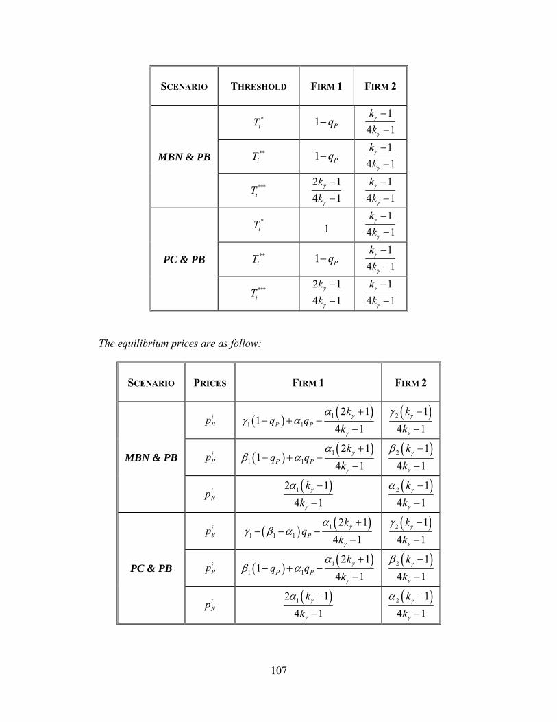
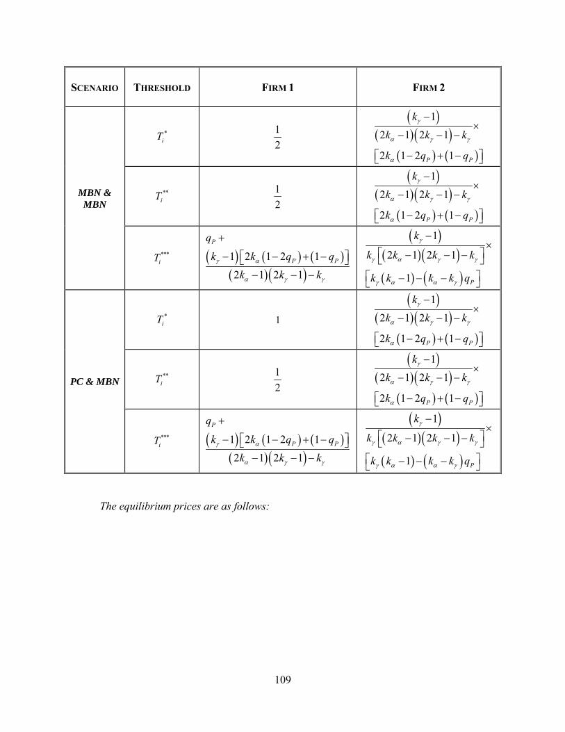
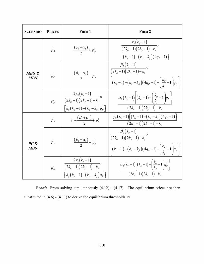
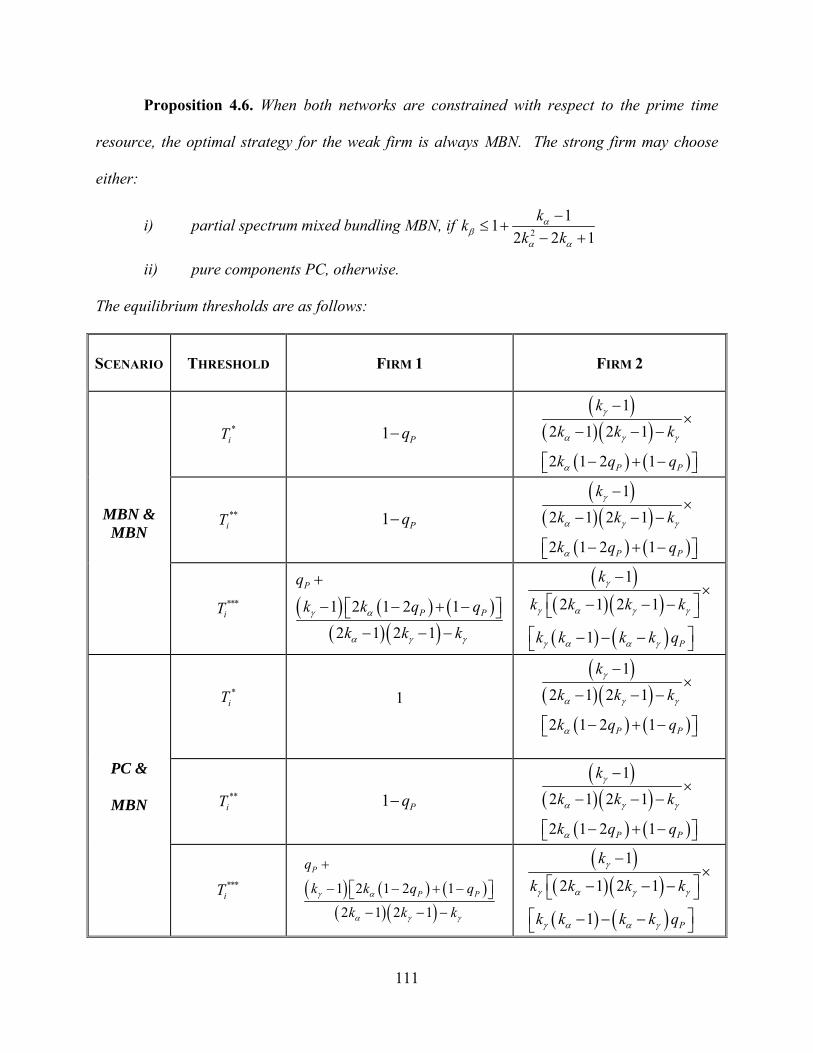
4.3 EQUILIBRIUM ANALYSIS ............................................................................ 97
4.4 VALUE OF BUNDLING WITH COMPETITION...................................... 113
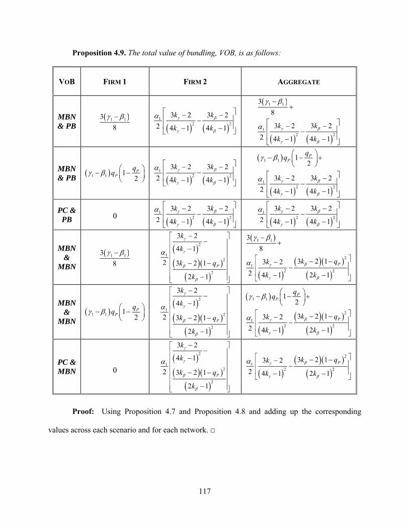
4.5 CONCLUSIONS AND EXTENSIONS .......................................................... 118
5.0 MIXED BUNDLING WITH INDEPENDENTLY VALUED PRODUCTS ...... 121
5.1 INTRODUCTION ........................................................................................... 121
5.2 SUBMODULAR OPTIMIZATION ............................................................... 123
5.3 THE GENERAL MIXED BUNDLING PROBLEM .................................... 125
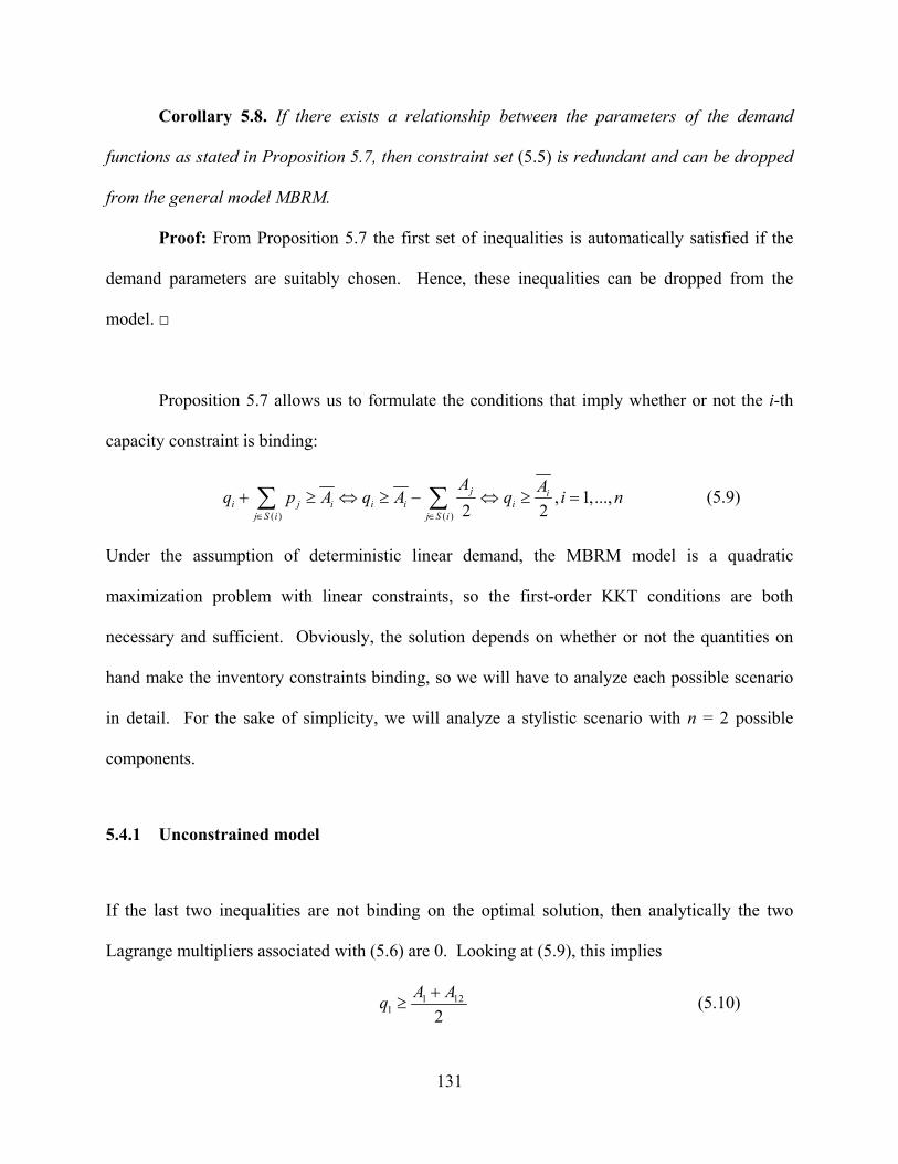
5.4 BUNDLING WITH LINEAR DEMAND FUNCTIONS ............................. 130
5.4.1 Unconstrained model ................................................................................... 131
Page 8
viii
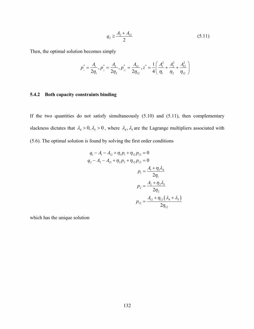
5.4.2 Both capacity constraints binding .............................................................. 132
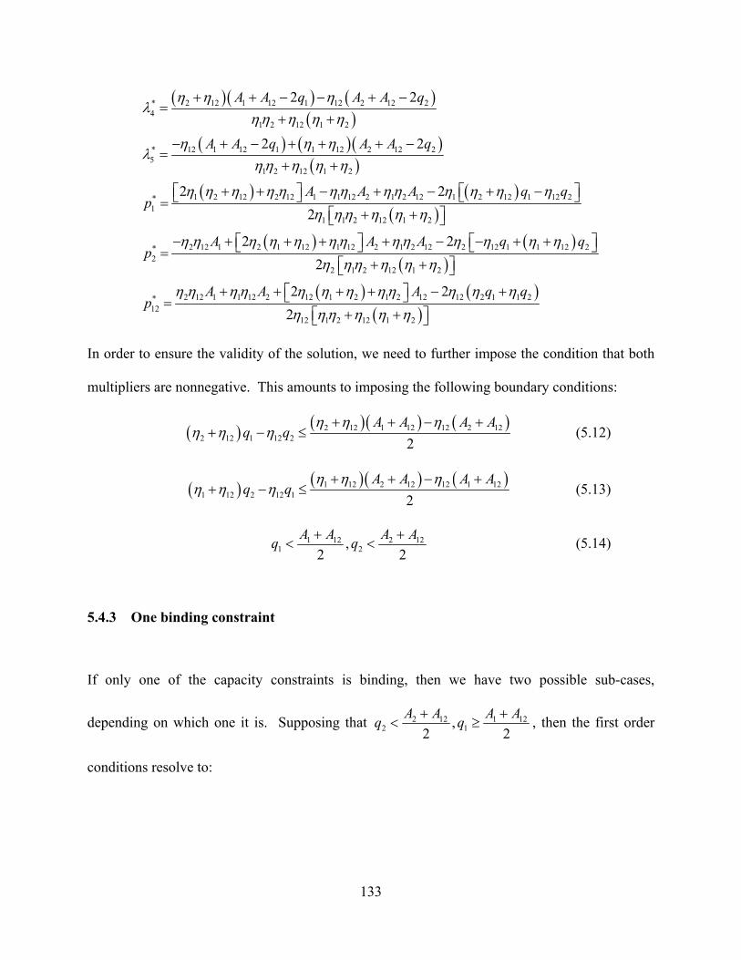
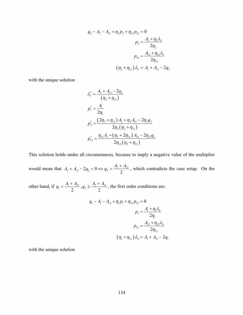
5.4.3 One binding constraint ................................................................................ 133
5.5 GREEDY HEURISTIC ................................................................................... 136
5.5.1 Worst-case heuristic performance ............................................................. 137
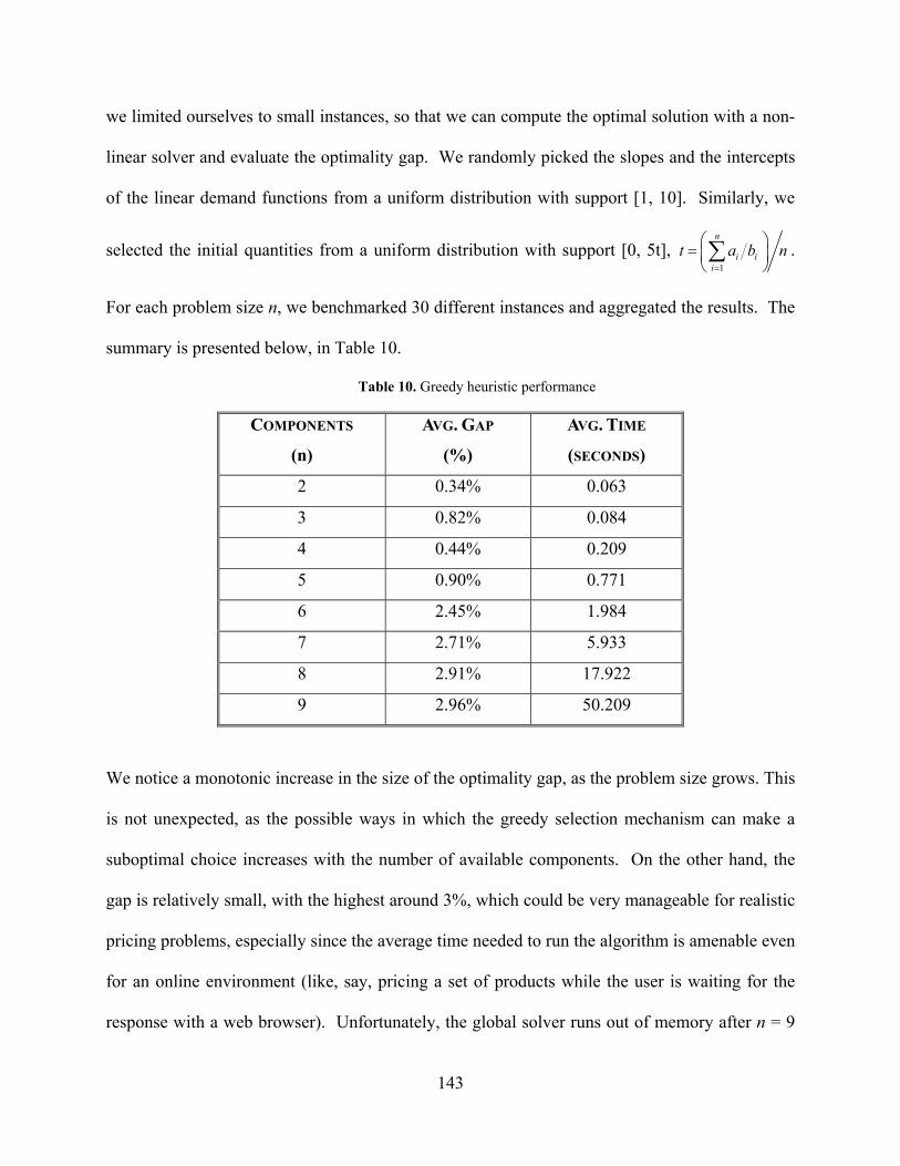
5.5.2 Computational results ................................................................................. 142
5.6 DECOMPOSITION FRAMEWORK ............................................................ 144
5.6.1 The restricted master problem ................................................................... 145
5.6.2 The separation sub-problem ....................................................................... 147
5.6.3 The pricing sub-problem............................................................................. 148
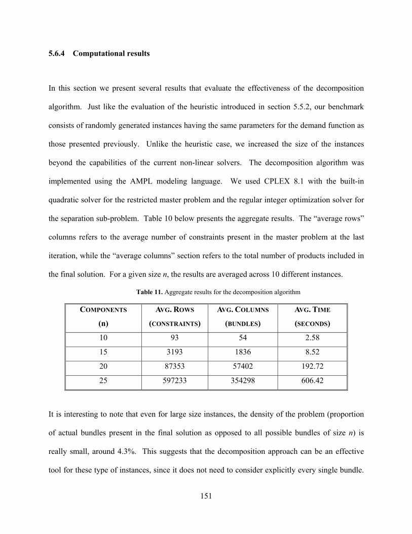
5.6.4 Computational results ................................................................................. 151
5.7 CONCLUSIONS .............................................................................................. 152
6.0 CONCLUSIONS AND FUTURE RESEARCH DIRECTIONS .......................... 155
BIBLIOGRAPHY ..................................................................................................................... 160
Page 9
ix
LIST OF TABLES
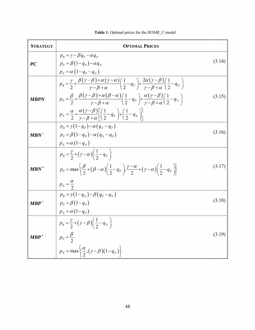
Table 1. Optimal prices for the ROMB_U model ......................................................................... 48
Table 2. Broadcaster’s VoB .......................................................................................................... 62
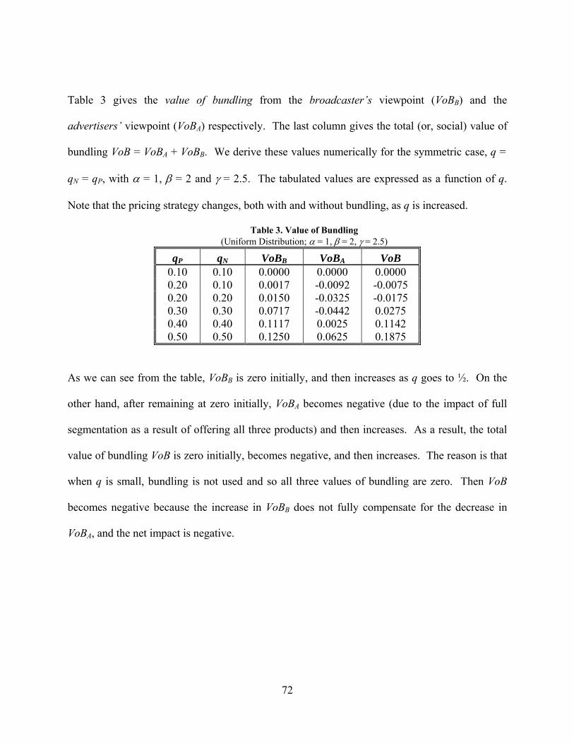
Table 3. Value of Bundling ........................................................................................................... 72
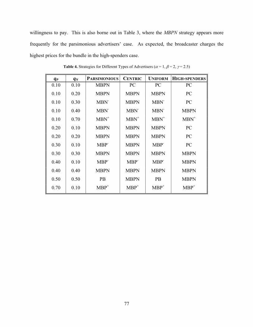
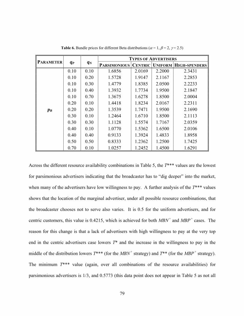
Table 4. Strategies for Different Types of Advertisers (α = 1, β = 2, γ = 2.5) ............................. 77
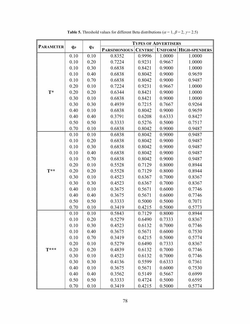
Table 5. Threshold values for different Beta distributions (α = 1, β = 2, γ = 2.5) ....................... 78
Table 6. Bundle prices for different Beta distributions (α = 1, β = 2, γ = 2.5) ............................. 79
Table 7. Broadcaster’s and aggregate value of bundling ............................................................ 114
Table 8. Advertisers’ and aggregate value of bundling .............................................................. 116
Table 9. MBRM problem growth for selected values of n ......................................................... 129
Table 10. Greedy heuristic performance ..................................................................................... 143
Table 11. Aggregate results for the decomposition algorithm .................................................... 151
Page 10
x
LIST OF FIGURES
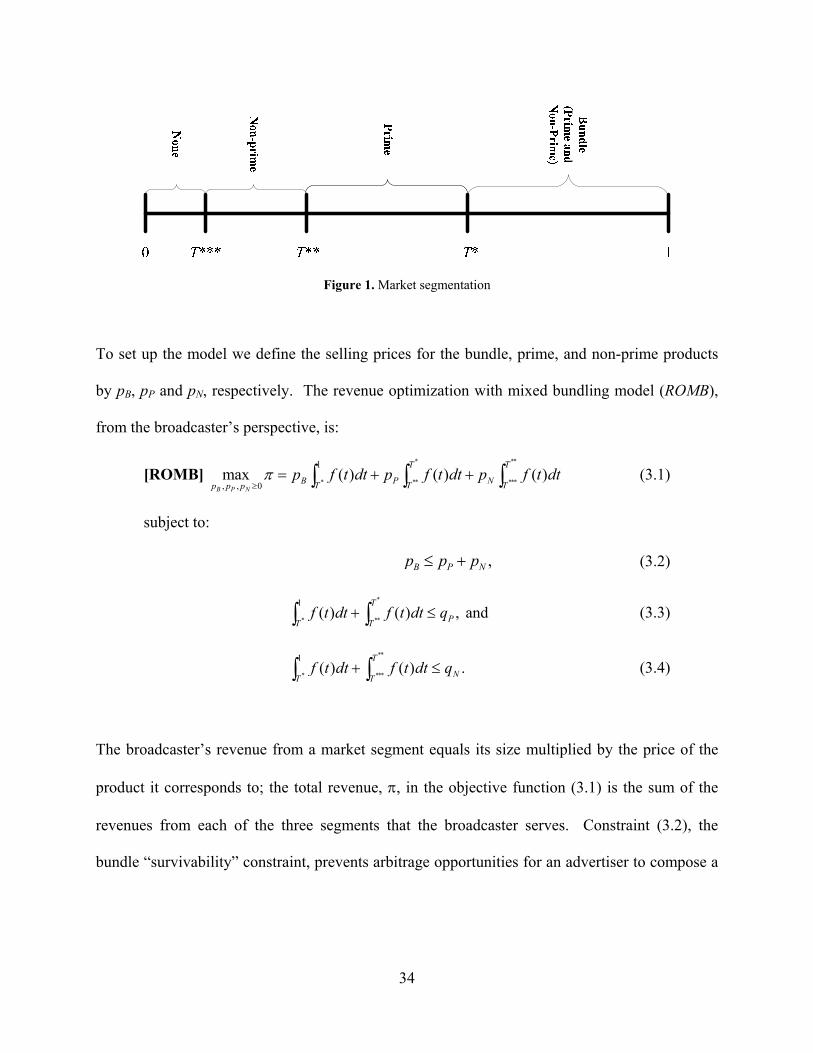
Figure 1. Market segmentation ..................................................................................................... 34
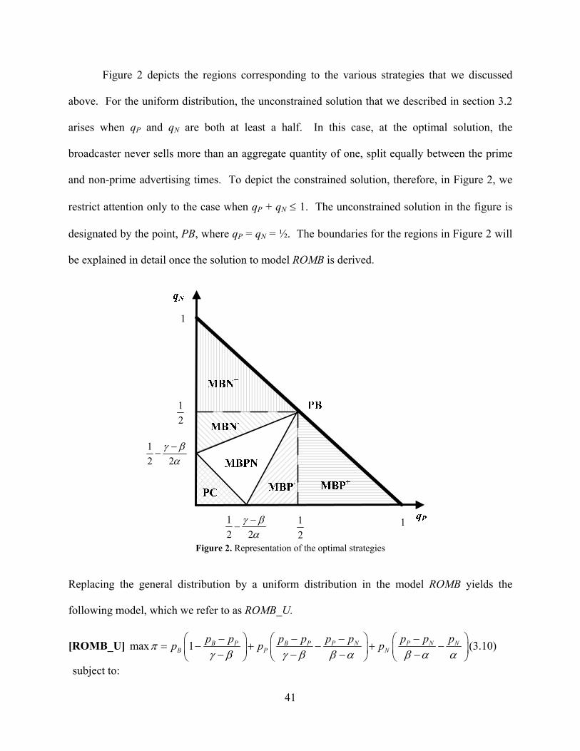
Figure 2. Representation of the optimal strategies ........................................................................ 41
Figure 3. Relative shadow prices of the resources for any ..................................... 52
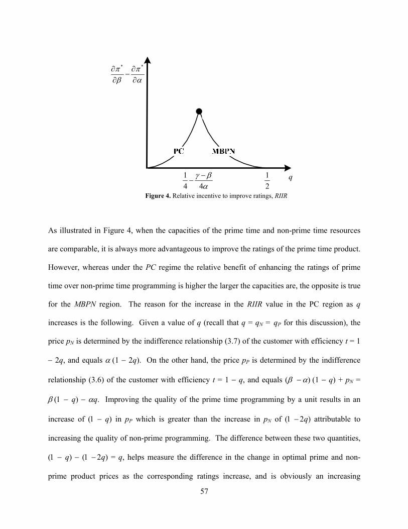
Figure 4. Relative incentive to improve ratings, RIIR .................................................................. 57
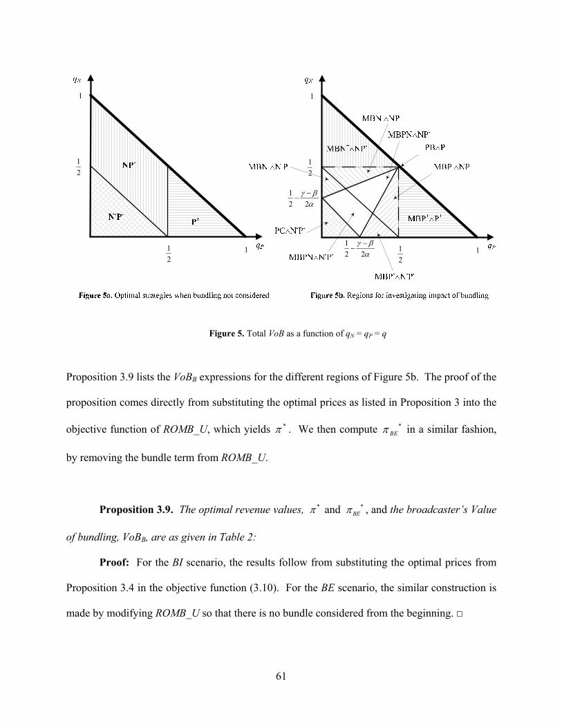
Figure 5. Total VoB as a function of qN = qP = q .......................................................................... 61
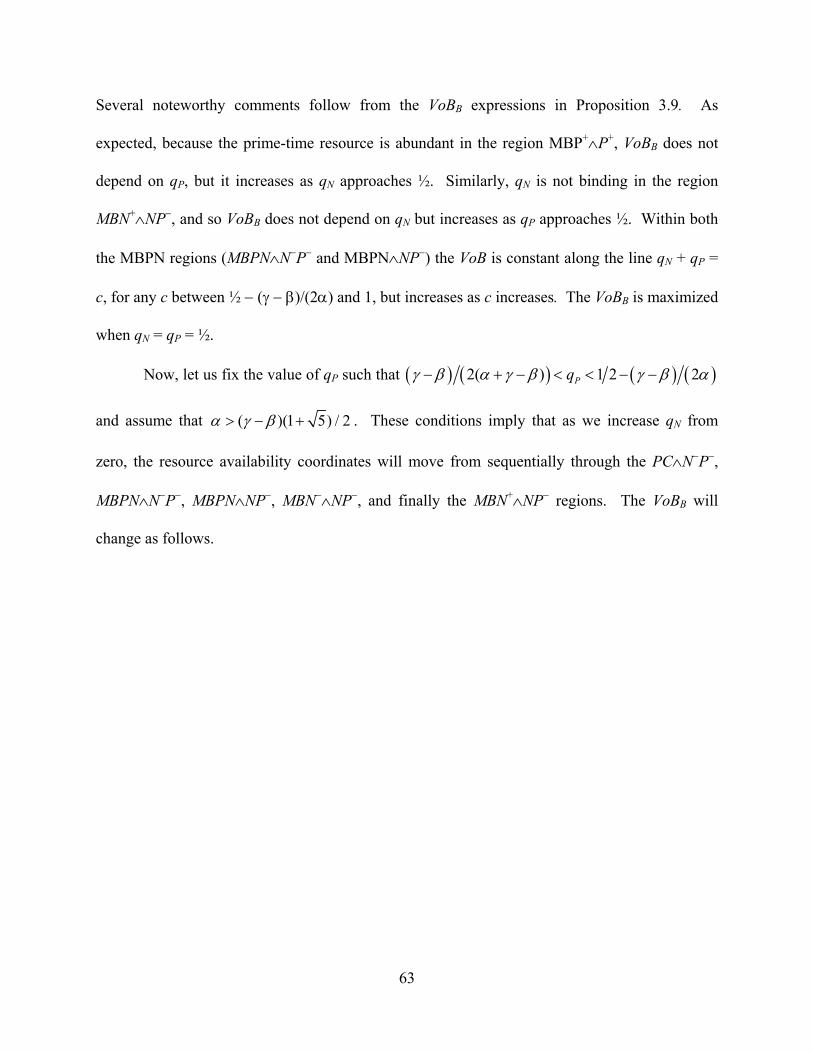
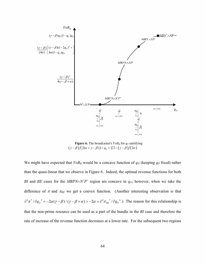
Figure 6. The broadcaster's VoBB for qP satisfying 64
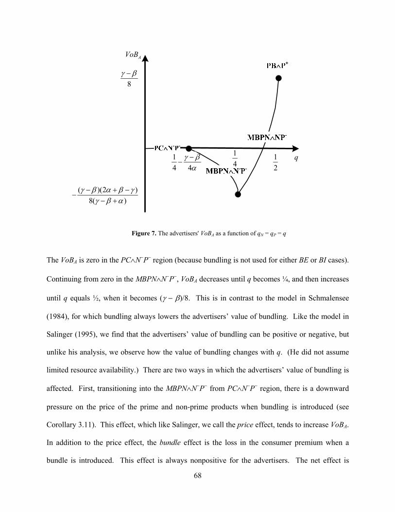
Figure 7. The advertisers' VoBA as a function of qN = qP = q ....................................................... 68
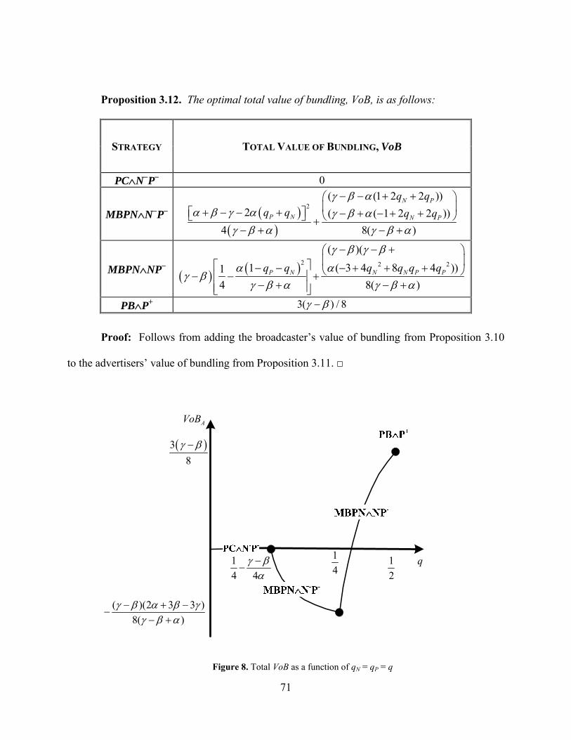
Figure 8. Total VoB as a function of qN = qP = q .......................................................................... 71
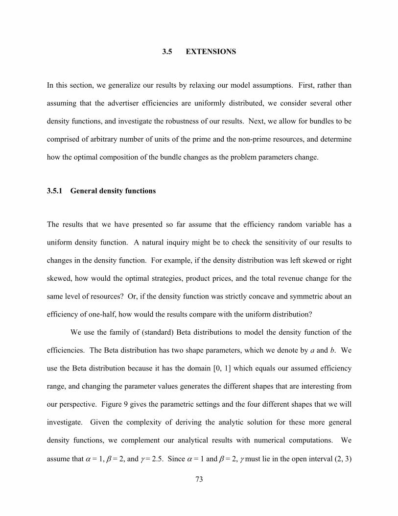
Figure 9. Density functions .......................................................................................................... 74
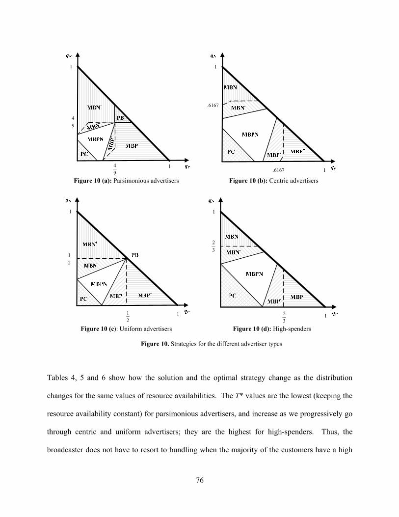
Figure 10. Strategies for the different advertiser types ................................................................. 76
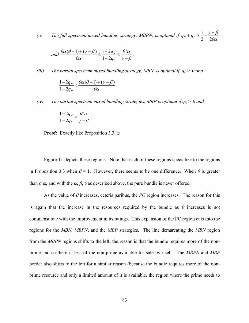
Figure 11. Optimal strategies as a function of the bundle composition parameter, θ .................. 84
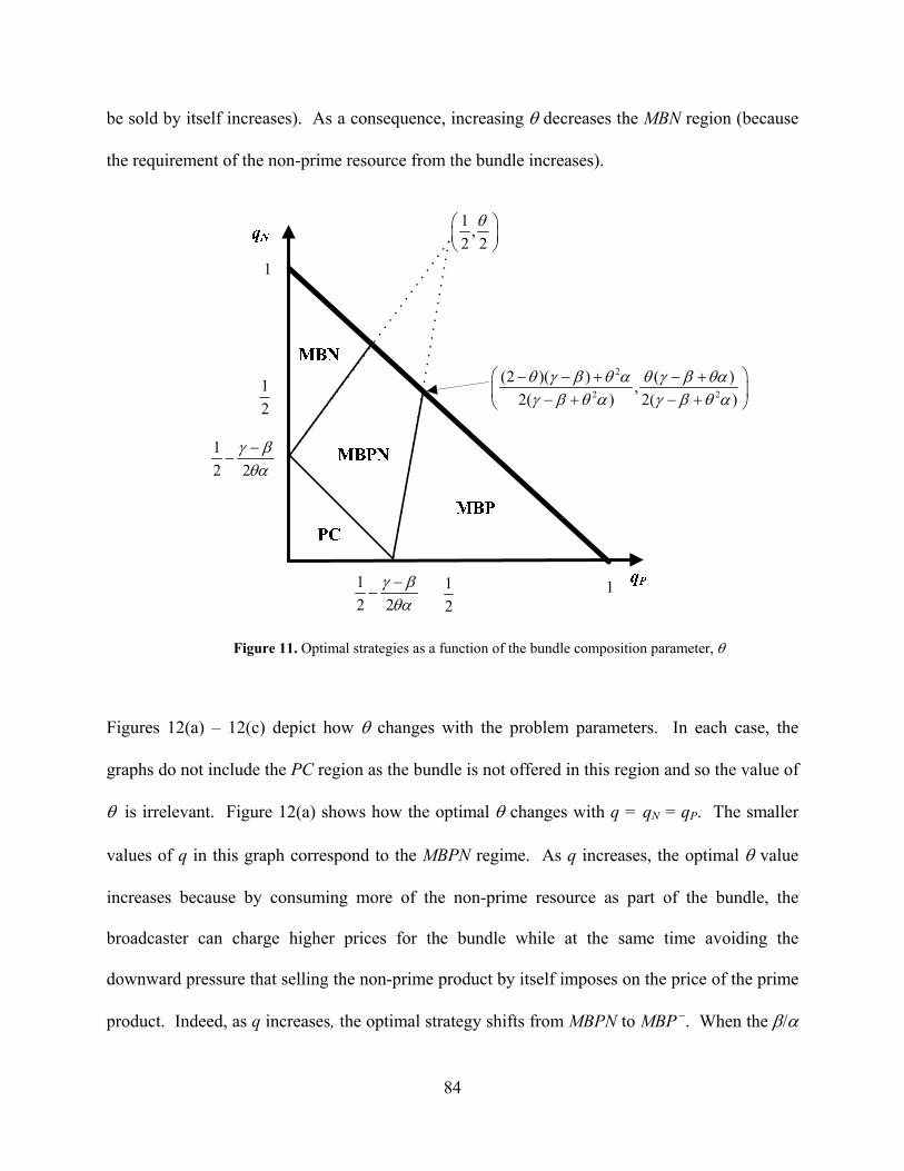
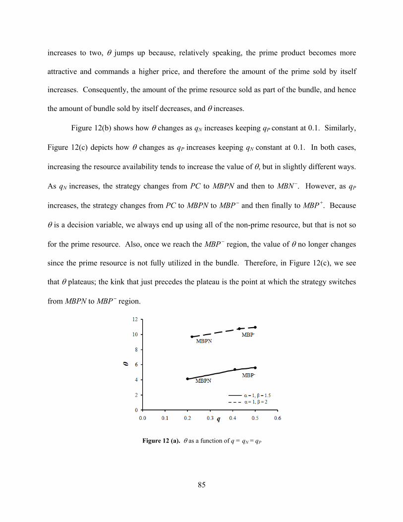
Figure 12. Change in θ with resource availability ........................................................................ 86
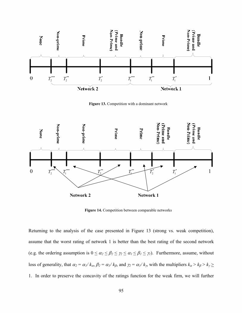
Figure 13. Competition with a dominant network ........................................................................ 95
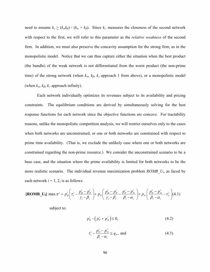
Figure 14. Competition between comparable networks ............................................................... 95
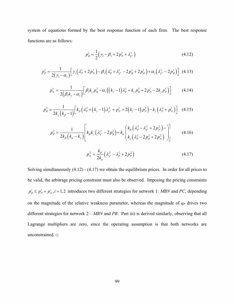
Figure 15. Valid equilibrium strategies ...................................................................................... 100
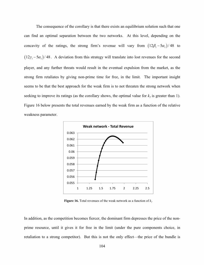
Figure 16. Total revenues of the weak network as a function of kγ ............................................ 104
1
2 2Pqγ β
α
−< −
( ) ( ) ( ) ( )2( ) 1 2 2Pqγ β α γ β γ β α− + − < < − −
Page 11
xi
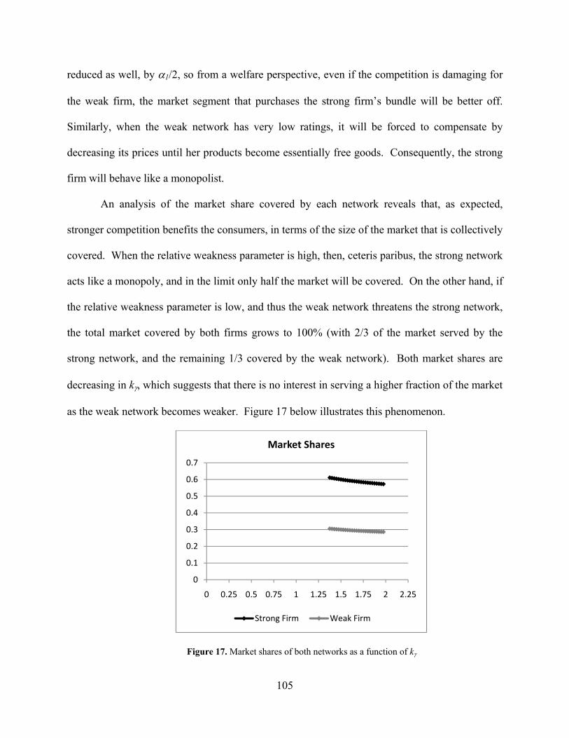
Figure 17. Market shares of both networks as a function of kγ ................................................... 105
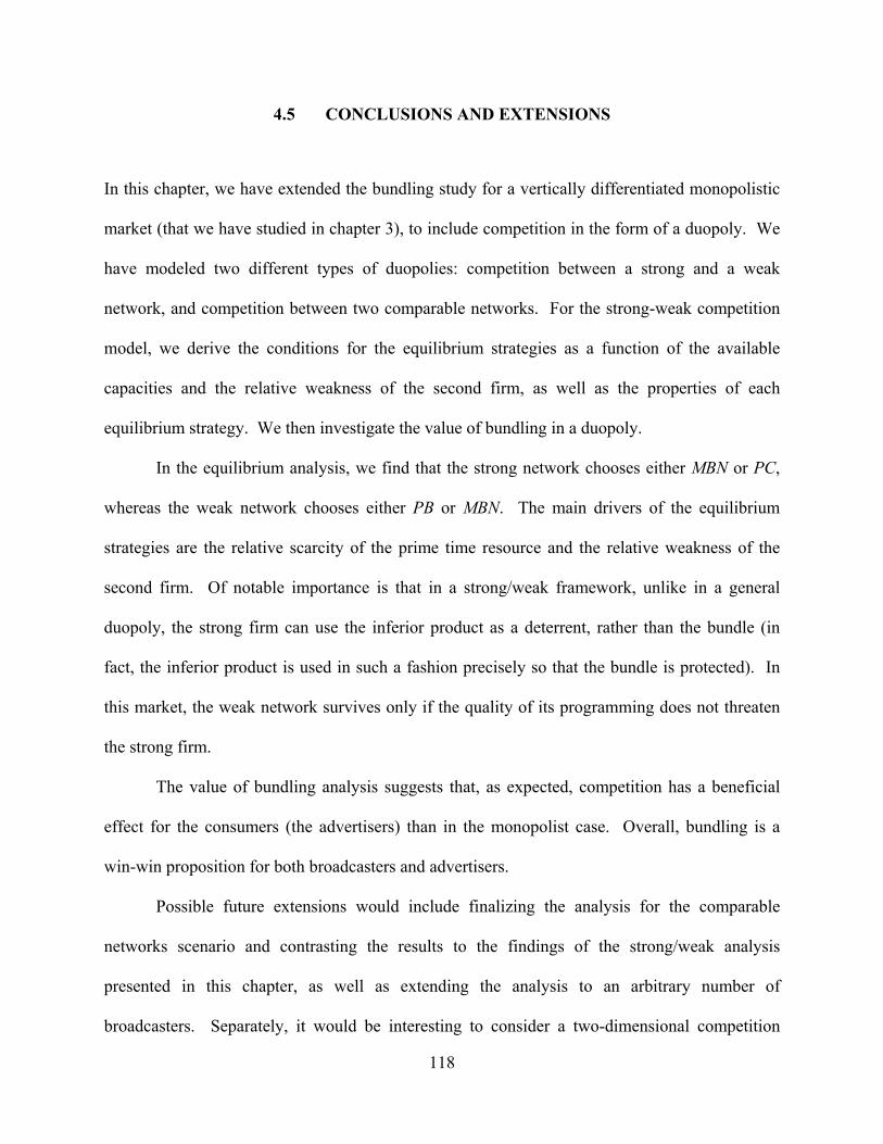
Figure 18. Two-dimensional competition model ........................................................................ 119
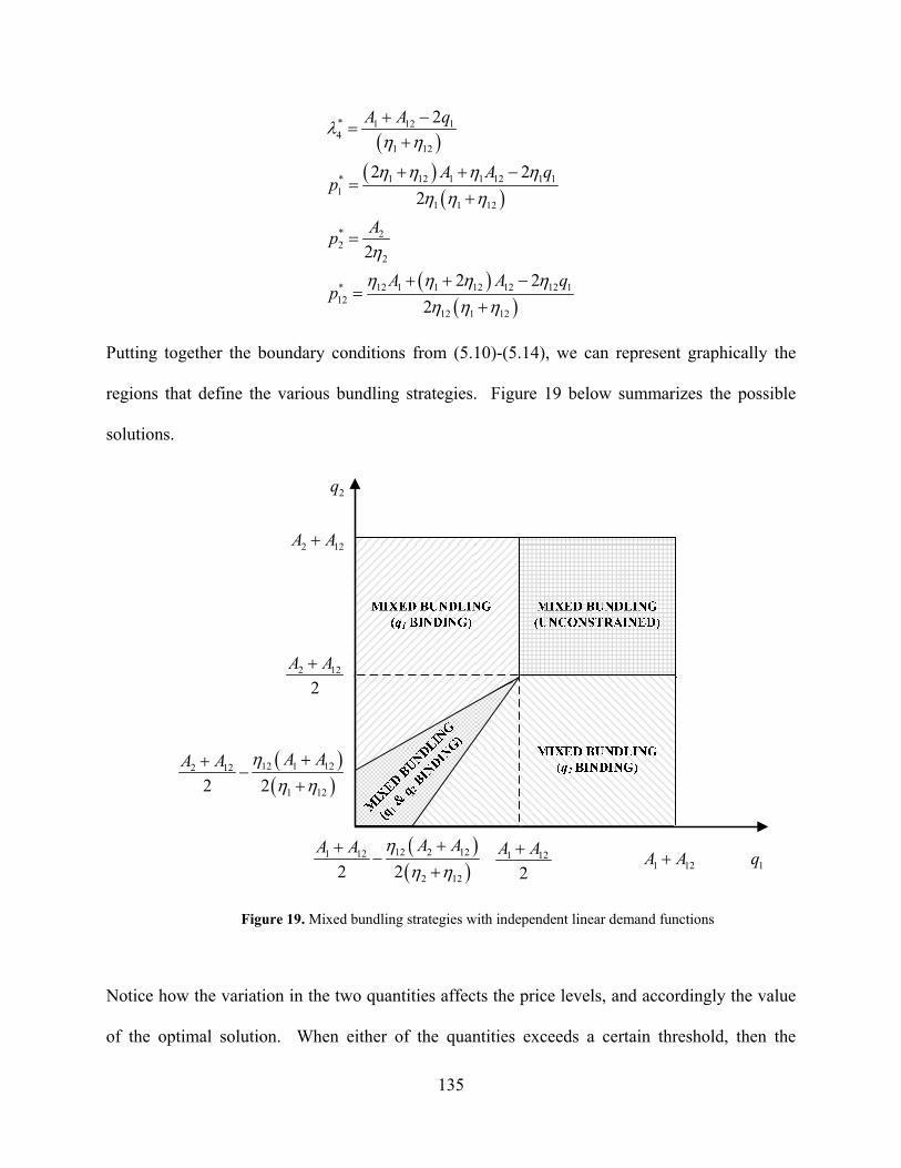
Figure 19. Mixed bundling strategies with independent linear demand functions ..................... 135
Figure 20. Description of the greedy allocation algorithm ......................................................... 137
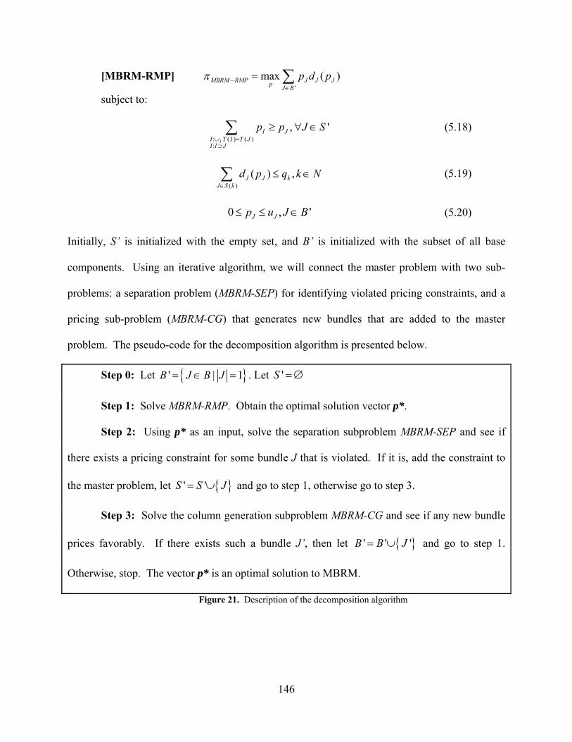
Figure 21. Description of the decomposition algorithm ............................................................ 146
Page 12
xii
ACKNOWLEDGMENTS
This work could not have been completed without the constant, significant support of my family,
my Pitt professors, and my friends. This is but a small token of appreciation for all the guidance
that I have received during this period.
First and foremost, I would like to thank my advisor, Professor Prakash Mirchandani, for
his mentorship, his supervision, his patience, and his willingness to help me at crazy hours. I am
inspired by you, and I hope that I have learned from your work ethic, and your character. I am
truly grateful for the opportunity to have worked with you.
My other committee members deserve a lot of thanks for this present work. I would like
to thank Professor Esther Gal-Or for her insights and her willingness to help develop this thesis;
her contribution was absolutely critical to the success of this dissertation. I am also grateful to
Professor Venkatesh for his helpful suggestions about bundling, and to Dr. Brady Hunsaker for
being a great teacher. Special thanks are in order for Professor Jerry May, who has been a great
role-model for me, for his wit, humor, personality, and guidance during the first years of the
program. I would also like to thank Dr. Srinivas Bollapragada for valuable discussions about the
problem addressed in this dissertation, and for his help in starting the computational work.
None of this would have been possible without the unconditional support of my family. I
would like to thank my wife, Alia, for her love, help, support, patience, understanding, and for
constantly being next to me through the highs and the lows. My parents, Liana and Ion, deserve
Page 13
xiii
all the thanks in the world for shaping me into what I am today, and for believing in my abilities.
This work is dedicated to all of you.
Finally, I would like to thank my friends for being there when I needed it. Scott and
Katie, thank you for being wonderful role models and friends, and for encouraging me to earn a
doctoral degree. Carrie, thank you for all your amazing help during these years. Radu, Jons,
Tudor, Dana, Victor and Silvia, and the rest of the Romanian gang—thank you for your
friendship. It’s what keeps us sane.
Page 14
1
1.0 INTRODUCTION
Across both service and manufacturing industries, a frequently used practice for increasing
revenue and profitability combines components (that is, individual products) into packages of
products. This strategy of selling packages, referred to as bundling, allows companies to satisfy
customers who may not be interested in buying the individual products, or who derive greater
consumer surplus from the packages than they do from the individual products. Thus, by
offering product bundles along with the components, a company can increase its market size by
appealing to a larger population. Bundling is also an effective instrument for price
discrimination, and presents opportunities for enhancing revenue without increasing resource
availability. Examples of bundling schemes include automotive option packages (for example,
bundling a navigation system with a premium audio system), vacation packages (for example,
bundling air, hotel and car rental reservations), software packages (for example, bundling word
processing and spreadsheet software), and food product assortments (bundling different flavors
of marinade sauces) and cosmetic products (for example, shampoo and conditioner, or mascara,
eyeliner and eye shadow, etc).
According to Stremersch and Tellis (2002), bundling manifests itself on a product basis,
where there is some degree of integration among the bundle components (e.g. the “quadruple
play” packages offered by telecommunication companies, which integrate phone, Internet,
television and mobile services), or on a price basis (e.g. season tickets for a sports team), where
Page 15
2
the absence of sufficient value-adding integration may require price-discounting. As these
examples indicate, a seller offering multiple components faces the following alternative
strategies (Adams & Yellen, 1976; Guiltinan, 1987): (i) pure-components strategy, in which the
seller only offers the components as separate items; (ii) pure-bundling strategy, in which the
seller only offers the bundle, but does not offer the components; and (iii) mixed-bundling
strategy, in which the seller offers both the components and the bundle(s). Our work examines a
mixed-bundling situation, and refers to both components and bundles as products. Given a
distribution of customers’ willingness to pay and the component availability, our objective is to
determine the revenue maximizing pricing strategy. We examine two different situations—
vertically differentiated versus independently valued products—and develop two different
approaches for revenue maximization opportunities using product bundling. For the vertically
differentiated market with two products, such as the television market with prime time and non-
prime time advertising, we derive optimal policies that dictate how the seller (that is, the
broadcaster) can manage their limited advertising time inventories, in a monopolistic as well as a
duopolistic environment. For the independently valued products assumption we analytically
derive optimal policies for the two components/one bundle scenario, and derive heuristics for
pricing arbitrary number of products.
In the context of TV advertising, broadcasters use a multi-pronged strategy to capture
revenues from the roughly $150 billion dollar advertising market in the US.1 The market for
selling television advertising time is split into two different parts: the upfront market, which
accounts for about 60%-80% of airtime sold and takes place in May every year, and the scatter
1 2007 TNS media intelligence report (http://www.tns-mi.com/news/03252008.htm). Of this amount, television
advertising accounts for roughly $64 billion annually.
Page 16
3
market which takes place during the remainder of the year. In the first stage of their strategy,
broadcast networks make decisions about how much advertising time to sell in the upfront
market and how much to keep for the scatter market. On their part, clients purchase advertising
time in bulk, guided by their medium-term advertising strategy, during the upfront market, at
prices that may eventually turn out to be higher or lower than the scatter market prices. The
scatter market, on the other hand, allows advertisers to adopt a “wait-and-see” approach to verify
the popularity of various network shows, and to tailor their decisions to match their short term
advertising strategy. In the television advertising market, capacity constraints play a significant
role in determining the broadcaster’s optimal strategy. Particularly, the relative scarcity of the
two resources, prime time and non-prime time, is the main driver of any sort of optimality
analysis. The prime time resource availability constraint is far more likely to be binding than the
non-prime time resource availability constraint. Prime time on television is usually the slot from
8:00 pm until 11:00 pm Monday to Saturday, and 7:00 pm to 11:00 pm on Sunday. Hence, the
ratio of prime to non-prime time availability is about 1:8 (or 1:6 on Sunday).
1.1 REVENUE MANAGEMENT AND PRODUCT BUNDLING
Due to the peculiarities of the TV advertising market, our work diverges from the current
revenue management stream in several ways. Traditionally, the revenue management literature
has focused on the airlines, hotels, cruise, automotive rental markets, and railway markets. In the
airlines, hotels, etc. situation, even though there is a strict ordering of the components, the bundle
may not be preferred to the “prime” product. For example, in the airline setting, an individual
may prefer a business seat to an economy seat on the same flight, but the individual is not likely
Page 17
4
to buy a bundle consisting of a both a business and an economy seat. Similarly, a traveler may
prefer a suite in a hotel to an ordinary double room on the same day, but is unlikely to rent a
bundle consisting of the suite and the double room. Likewise, an executive may prefer a full-
size car to a compact during the same trip, but is unlikely to rent both the full-size car and the
compact. This is quite different from a vertically differentiated market (e.g. the TV advertising
market) where all advertisers prefer buying a bundle of prime time advertising and non-prime
advertising to buying just prime time advertising, and prefer buying prime time advertising to
buying just non-prime advertising.
The advertising market is different from other revenue management applications in
another way. A “bundle” in the airlines industry could be two flight segments. Consider three
demands: Pittsburgh to New York, New York to Boston, and Pittsburgh to Boston. Airline
revenue management applications might consider a bundle of Pittsburgh to New York and New
York to Boston to meet the Pittsburgh to Boston demand. But clearly a preference order does
not exist in this case for the traveler: in fact the bundle may have lower utility than the Pittsburgh
to New York product for someone wanting to travel to New York from Pittsburgh. Similar
situations also occur in the hotel industry where a bundle may consist of a hotel room on Sunday
and a hotel room on Monday. A business traveler, wanting to spend Sunday night with her
family might have no interest in purchasing the bundle. So, in these cases, consuming the bundle
may have lower utility than consuming the individual components.
The methodologies developed and the approaches adopted in the revenue management
literature are also different from our work. While the revenue management literature is quite
extensive, none of the revenue management papers adopt the “market segmentation through self
selection” (that is, second degree price discrimination) approach as we do in this work. On the
Page 18
5
contrary, “fences” (Saturday night stay requirement to prevent a business traveler from using a
leisure fare, or a student id requirement to prevent a regular patron from buying a discounted
concert ticket) are typically constructed to prevent spillage. Moreover, in most revenue
management papers, the prices are exogenously given rather than endogenously determined, as
in our work. While there are papers that consider simultaneous pricing and inventory
management decisions (Dana Jr & Petruzzi, 2001; Petruzzi & Dada, 1999; Raz & Porteus, 2006),
multiple components and/or the availability of a bundle are not considered in these papers at all.
Finally, according to Bollapragada and Mallik (2008), Zhang (2006), and Araman and
Popescu (2009), the current practice in the broadcasting industry is to use subjective methods for
media planning decision, and only a few analytical models have been developed. Talluri and van
Ryzin (2004), the most up-to-date, comprehensive reference on revenue management, describes
some scheduling models for this application context. Araman and Popescu (2009) suggest that
technical complexity argues for decomposing the general media planning problem into smaller,
tractable problems, and consider allocating advertising time capacity between the upfront and
scatter markets given the uncertainty of the audience. Bollapragada and Mallik (2008) focus on
how to manage the “rating points” inventory for servicing the upfront market. Zhang (2006)
develops a hierarchical approach for matching advertisers to shows and then constructing a
broadcast schedule. Up to this point, none of these recent articles, as well as other recent
television media related papers, consider the issue of bundling problem applied onto the TV
advertising market.
Page 19
6
1.2 OBJECTIVES OF THIS WORK
The current thesis aims to address two major issues. The main contribution of this research is to
study the effectiveness of various bundling strategies on a market characterized by ordered
preferences (i.e., the TV advertising market). Here, we show how the various strategies shift as a
function of the advertising time inventory, and we also study the impact of the distribution of
clients over the overall profitability of the TV network. Chapters 3 and 4 of the dissertations
study this problem under different assumptions. In Chapter 3, we start with a monopolistic
framework, and we assume that the buyers (in this case, the advertisers interested in purchasing
advertising time) self select into different segments (non-purchasers, buyers of only one type of
advertising product, or buyers of bundles containing both the “lower quality” and the “higher
quality” product). In the TV context, the “lower quality” time is called non-prime time and the
“higher quality” time is referred to as prime time. The availability of these two resources is
limited. Traditionally, the bundling research has consistently found that mixed bundling
strategies dominate other bundling strategies, because a bundle is able to capture extra revenues
by reducing the heterogeneity of the consumers. Moreover, the issue of whether bundling
benefits only one player (buyer or seller) involved in the transaction, or whether bundling is a
win-win proposition when the resource availability is limited, is not addressed in the literature.
Our work in Chapter 3 seeks to investigate these issues in the TV media context, and see whether
conventional wisdom with respect to bundling holds, or whether the intrinsic characteristic of
this market induces a different behavior. Additionally, we are also interested in finding out as to
what are the incentives for improving programming quality in the context of selling bundles of
prime and non-prime time. In Chapter 4, we address the same questions but this time in a
Page 20
7
duopolistic setting. Hence, Chapter 4 extends the results of Chapter 3. Overall, the contributions
of the first two essays can be summarized in the following main discussion points:
The pure components strategy may dominate the mixed bundling strategy. Past bundling
literature in a monopoly setting (Adams & Yellen, 1976; McAfee, McMillan, & Whinston, 1989;
Stigler, 1963) has demonstrated that the mixed bundling strategy (weakly) dominates the pure
components and the pure bundling strategies for independently valued components. We
investigate the generality of this result and show that when all customers have a common
preference ranking of the products, and the resource availability is unconstrained, then the pure
bundling strategy is optimal. More importantly, we show that with constrained resource
availability, the optimal strategy depends on the scarcity of the resources. In particular, we show
that the pure components strategy may be the optimal strategy, dominating the mixed bundling
strategy, when the resource availabilities are low. Thus, the clean, unambiguous structure of the
optimality of the mixed bundling strategy breaks down when the preferences for the products are
ordered and the resources are limited.
The skewness of the customer distribution is important in addition to its heterogeneity.
Schmalensee (1984) points out that the reason for the dominance of the mixed bundling strategy
stems from the fact that it allows greater price discrimination by reducing the heterogeneity of
the customers. Our results show that the skewness of the distribution of customers, in addition to
the heterogeneity, affects the benefits of mixed bundling. To our knowledge, previous research
has not studied the impact of skewness on bundling.
Should programming quality be improved? If so, which one? One question that effective
managers always ask is how they can do better: in this case, how can the broadcasters’ profit be
increased? Should we try to improve the ratings of the prime time or the non-prime time
Page 21
8
programming? We answer this question by concluding that, under fairly mild additional
assumptions, it is always (that is, under all bundling strategies) better to improve the ratings of
the resource that is more plentiful. Additionally, when the availabilities of the two resources are
equal to each other, it is always better to increase the ratings of prime time programming, but the
relative benefit from quality improvement of prime time programming depends on the overall
resource scarcity.
Does bundling in our context improve consumer and social welfare? When decision
makers evaluate a new strategy, they need to consider not just what the impact on their bottom
line would be, but also how customers and society, in general, would be impacted. Are there
situations where everyone (in this case, the broadcaster and the advertisers as a group) would be
better off? We answer this question in the affirmative by computing the value of bundling for
the broadcaster, the advertiser, and aggregate, in both monopolistic and duopolistic settings. The
consumer and social welfare measures have been studied in other contexts, and sometimes a
similar phenomenon has been observed. However, the relationship of the value of bundling to
the scarcity of resources, and as a result, to the optimal bundling strategy, has not been addressed
at all in the literature.
In a competitive environment with a strong (in terms of ratings) network and a weaker
one, the strong network uses the non-prime time product as a deterrent. Previous literature on
bundling in competitive environments has shown that the bundle can be used as a deterrent
(Nalebuff, 2004). Our work suggests that in a vertically differentiated product market with a
weak and a strong player, the strong firm uses the lower quality bundle component as a deterrent,
because in the limit it can be sacrificed and given away for free (the marginal costs are zero in
our model), in order to protect the bundle.
Page 22
9
In the final essay, we depart from the vertical differentiation model and study the general
mixed bundling problem. Here, we formulate the general mixed bundling problem under both
stochastic and deterministic demands, and investigate the properties of the deterministic
approach. We can summarize the contributions of this work along the following discussion
points:
We investigate the connections between the optimal bundling strategies for vertically
differentiated and independently valued products. We show analytically that the regions defined
by the number of binding capacity constraints are similar in both situations. However, the
dominant strategies are very different within each such region. (As we will discuss later, the
assumptions underlying the two situations are quite different.)
We analyze effective solution methodologies for large-scale versions of the mixed
bundling problem. We investigate two different approaches that are computationally efficient: a
generic greedy heuristic for pricing arbitrary bundles of products with independent valuations,
and a decomposition method. We investigate the theoretical performance of the heuristic, and
observe that in practice it tends to perform well for moderate-sized problems. Then, we
formulate and evaluate a decomposition method that is geared towards large-scale problem
instances. We find that, in our limited computational experiments, on average more than 99.9%
of the constraints of the optimization model are naturally satisfied by the solution, and therefore,
it is possible to save valuable computational time by doing an implicit, rather than explicit
enumeration of all the model constraints. Even more interesting, only a fraction of all possible
bundles end up being offered in practice. With careful selection rules which we expand upon in
Chapter 5, we can save a lot of computational time by identifying these candidates. Therefore,
Page 23
10
the overall theme of this last essay is the development of efficient algorithmic approaches for this
hard combinatorial problem.
1.3 OVERVIEW OF CHAPTERS
Following this introductory chapter, the second chapter provides an overview of the current
research stream, as it is applicable to revenue management and product bundling. This chapter
builds an introductory foundation upon which this work can extend the current state of the art.
Subsequent chapters will address relevant research literature in a more focused manner, in their
corresponding introductory sections.
Chapter 3 examines a basic monopolistic setting in which the TV network seeks to
maximize its revenues from sales of limited prime and non-prime advertising time, using
different bundling strategies. We examine the impact of the relative scarcity of advertising time
on the different strategies, quantify the effect of the shadow prices on the bundle composition,
and look at the network relative incentive to improve the programming quality (and thus, its
ratings). We show how changing the distribution of the customers affects our results. We also
show how the value of bundling changes (the value of bundling is the net benefit for both the
advertisers and the network) as the relative availability of the two advertising time resources
changes.
Chapter 4 extends the monopolistic framework to a competitive duopolistic environment.
We examine the impact of competition on the bundling strategies, and we also quantify the value
of bundling. We present and interpret several structural properties of the value of bundling
Page 24
11
function, and show that there exist certain scenarios where bundling is a win-win proposition for
all parties.
Chapter 5 approaches the bundling issue when the products are independently valued
with known demand curves. We also provide a heuristic approach that generates near-optimal
solution to the revenue maximizing mixed bundling problem, and conclude with a worst-case
behavior analysis of its performance, along with several computational experiments. Finally, we
introduce a decomposition-based framework that efficiently solves large scale instances of the
mixed bundling problem, formulated as a convex optimization program.
Finally, Chapter 6 is a summary of the work developed in the thesis, with discussion on
limitations and plans for improvement and extensions.
Page 25
12
2.0 REVENUE MANAGEMENT AND PRODUCT BUNDLING
Businesses that sell perishable goods or services often have to manage a relatively fixed
inventory of a product over a planning horizon. Revenue management (sometimes also referred
to as demand management) is the active administration of all processes that could generate extra
revenues from an existing inventory (or in some cases, capacity), by making better decisions
with respect to pricing and/or allocation of a particular (or an entire line of) good(s) or service(s)
that the company is offering. Organizations that use revenue management techniques often
employ various techniques, such as priority rules for inventory allocation, customer
segmentation, forecasting, and the dynamic adjustment of prices. Successful implementations of
revenue management techniques have led to increased revenues and profits for many
organizations across various industries, most notably airline, hotel, restaurant and car-rental
businesses. Opportunities are now arising for the introduction of revenue management
techniques into non-traditional areas, such as healthcare and the entertainment and advertising
industries. Making decisions about the prices to charge and the availability of those products or
services for each market segment over a period of time with the goal of increasing the expected
profit pertains to revenue management. Thus, revenue management is sometimes referred to as
“the art of maximizing the profit generated from managing a limited capacity of a product over a
finite horizon, by selling each product to the right customer, at the right time, for the right price.”
(Talluri & Van Ryzin, 2004)
Page 26
13
One of the major pillars supporting the revenue management foundation is the concept of
market segmentation into multiple classes (e.g., leisure versus business travelers), where
different types of products (e.g., seats on an airline with restricted or fully refundable fares) are
targeted to each class. Another important operational driver is the idea that some resources are
perishable. A resource is perishable if after a certain date becomes either unavailable or it ages
at a significant cost. Seats on a flight or in a theater, rooms in a hotel, space on a cargo train, are
a few examples of such perishable inventory, so the main focus of revenue is on the allocation of
limited and perishable capacity to different demand classes (Elmaghraby & Keskinocak, 2003).
Revenue management, or yield management as it was initially called, started in the airline
industry, back in the late 1970s, as a need for airline companies to cope with the increased
competition when many fares became available, following the Airline Deregulation Act of 1978.
Airlines had to manage the discounted fares that became part of their product offers, and the
opportunities for revenue management techniques and models were acknowledged very fast.
Their positive impact on revenue was attested by many companies. For example, American
Airlines had a $1.4 billion in incremental revenue over the three year period between 1989-1992
(Smith, Leimkuhler, & Darrow, 1992). Recent successful applications of revenue management
principles span industries beyond airlines. For example, Geraghty and Johnson (1997) report
that successful revenue management saved the National car rental company from bankruptcy. In
another study, Bollapragada et al. (2002) report significantly improved revenues after optimizing
NBC’s commercial scheduling systems, and Metters et al. (2008) report the successful
application of revenue management-based segmentation at Harrah’s Cherokee Casino. Other
interesting applications of revenue management can be encountered in car rental businesses
(Savin, Cohen, Gans, & Katalan, 2005), media advertising (Araman & Popescu, 2009;
Page 27
14
Fridgeirsdottir & Roels, 2009), internet service providers (Nair, Bapna, & Brine, 2001), cargo
shipping (L. H. Lee, Chew, & Slim, 2007; Pak & Dekker, 2004), and restaurants (Kimes, 1999).
The most comprehensive survey articles that encapsulate the past literature and main results in
revenue management are, chronologically, those of Weatherford and Bodily (1992), McGill and
van Ryzin (1999), and Talluri and van Ryzin (2004).
Traditionally, revenue management research is broadly split along two dimensions. The
quantity based revenue management is mainly concerned with capacity allocation decisions. In
the airline case, for example, one of the tactical decisions is to determine the number of seats to
make available to each fare class from a shared inventory and how many requests from each
class to accept, in order to maximize total expected revenues, taking into account the
probabilistic nature of future demand for a flight (Belobaba, 1989). In other words, given a
booking request for a seat in an itinerary in a specific booking class, the fundamental revenue
management decision is whether to accept or reject this booking, considering the past and future
demands. In the hotel industry, the manager has to decide at the operational level, for example,
whether or not to rent a room to a customer that requests it, considering the reservations already
made, future reservation requests, and the potential walk-ins (customers that show up without a
reservation). So it is not at all uncommon to deny an advanced booking (in either business) to
price-sensitive customers for peak travel periods because it is anticipated that there will be
enough demand from higher paying customers. The analysis of capacity (seat) allocation, (that
is, controlling the mix of discount fares and early booking restrictions) and overbooking (selling
more seats than available when cancellations and no-shows are allowed) are supported by a
thorough understanding of customer behavior and the capability to accurately forecast future
demand. The three most important airline and hotel revenue management interrelated aspects
Page 28
15
and areas of research are forecasting, seat allocation and overbooking. On the other hand, the
price based revenue management is concerned with pricing decisions. These decisions can be
different, depending on the industry. For example, in the airlines and the hotel industry, one
form of control is that of bid prices, where the request for a seat (or a room) is accepted only if
the price offered exceeds a threshold established by the seller (for example, in the airlines
industry the most common way to compute a bid control for a flight is to sum the dual prices of
all the capacity constraints associated with each leg of that particular flight). In the retail
industry, an efficient form of price control is that of markdown pricing, where, at certain time
intervals during the season, the prices for different items are permanently reduced. Finally,
across various industries, an efficient technique is that of dynamic pricing, which refers to the
adjustment of prices (either upwards or downwards) at various moments during the planning
horizon.
Revenue management is attributable to bringing new ideas and models that changed the
paradigm about doing business. In one form or another, revenue management applications and
their consequences are felt more and more, be it when renting a hotel room or a car online or
trying to find a deal in a superstore by buying a bundling of products. Revenue management is
actively trying to reach new business settings and one of the current research focuses is finding
ways to better incorporate customer behavior, lifetime customer value and competitive response
into the revenue management decisions (Phillips, 2005).
Page 29
16
2.1 BUNDLING STRATEGIES
Bundling is a prevalent business strategy. Most of the bundling papers are built on the early
study of Stigler (1963), who concludes that bundling is profitable when the reservation prices of
the components are negatively correlated. Later, Adams and Yellen (1976) show that the
profitability of bundling can stem from its ability to sort customers into groups with different
reservation price characteristics, thus extracting greater consumer surplus. They examine the
three basic bundling strategies (pure components, pure bundling, and mixed bundling), compare
these strategies in terms of seller profit and find that mixed bundling at least weakly (meaning
that the revenues collected from a mixed bundling strategy are at least as high as those collected
if some other strategy were followed) dominates pure bundling, since customers with negatively
correlated reservation prices prefer individual products, while the others prefer the bundle. A
related paper, (Dansby & Conrad, 1984) finds the same effect, as well as the study made by
McAffee, McMillan and Whinston (1989). Bundling can also be used strategically, as an entry
barrier, as Nalebuff (2004) shows in a recent paper.
Schmalensee, in two early papers (1982, 1984) relaxes the assumption that the
reservation prices of the individual products are negatively correlated, and examines the case of a
monopolist offering two products. He constructs a class of examples within which the
profitability of bundling can be analyzed as a function of production costs, the mean and
variance of the distribution of reservation prices for each product, and the correlation between
the reservation prices of the two products. Schmalensee also demonstrates that mixed bundling
combines the advantages of pure bundling and pure components strategies, because this policy
enables the seller to reduce effective heterogeneity among those buyers with high reservation
prices for both goods, while still selling at a high markup to those buyers willing to pay a high
Page 30
17
price for only one of the goods. An interesting consequence is that bundling can be profitable
when demands are uncorrelated or even positively correlated.
Keeping it in the same two-product scenario, Venkatesh and Kamakura (2003) examine
the relationship between the products—that is, whether they are complements, substitutes, or
independent—and derive analytical solutions, based on the bivariate uniform distribution of
consumers’ reservation prices, for pricing either a pure bundle or the components separately, and
do a numerical simulation for the mixed bundling scenario. Earlier, while examining a situation
within the entertainment industry (pricing season tickets for an event), Venkatesh and Mahajan
(1993) determined that mixed bundling can dominate both pure bundling and components
strategies under certain conditions of the prices. They also derive analytical and numerical results
for the profit maximizing equations when the probability density function that describes the
customers’ reservation prices follows a Weibull distribution.
Bakos and Brynjolfsson (1999) study the strategy of bundling a large number of
information goods (that have zero marginal costs), such as those increasingly available on the
Internet, and selling them for a fixed price. Interestingly, they find that bundling very large
numbers of unrelated information goods and offering only the bundle (that is, a pure bundling
strategy) can be surprisingly profitable, and can dominate the mixed bundling strategy. This
research contrasts with the physical bundling scenario, where a negative product correlation
seems to be the main driver of mixed bundling profitability. In a latter paper (2000), the same
authors extend their research to a general competition model on the Internet via bundling.
Keeping the same approach, Altinkemer (2001) examines the bundling strategy in the online
environment of e-banking strategies.
Page 31
18
Salinger (1995) focuses on the graphical analysis of bundling and deals with the two-
product case, while assuming additive reservation prices. He explores the implications of the
relationship between the bundle and aggregated components demand curves for the profitability
and welfare effects of bundling, and finds that if it does not lower costs, bundling tends to be
profitable when reservation values are negatively correlated and high relative to costs. If
bundling lowers costs and costs are high relative to reservation values, positively correlated
reservation values increase the incentive to bundle. On the other hand, Soman and Gourville
(2001) illustrate how the bundling of services can hurt consumption, due to its nature of hiding
costs from consumers (they argue that bundling increases the valuation complexity).
The internal valuation of bundles is a well-established marketing research area (Yadav,
1994; Yadav & Monroe, 1993). Chung and Rao (2003) examine the valuation of bundles
comprised of heterogeneous products that could belong to several categories, and its implication
on any optimal bundle pricing. For an ample study of factors that drive bundle purchase
intentions, the handbook of Fuerderer, Herrmann and Wuebker (1999) provides a comprehensive
treatment of the subject.
One notable shortcoming of most of these research papers is the relatively small number
of optimal bundle prices derivations. One important study that examines this topic is the paper
of Hanson and Martin (1990) which provides a practical method for calculating optimal bundle
prices. The basis of the approach is to formulate the model as a mixed integer linear program
using disjunctive programming. The authors also consider one of the most serious problems
facing a product line manager addressing the bundling issue: the exponential growth in possible
bundles which results from increasing the number of components considered. An algorithm for
finding optimal solutions is given along with computational results. A different approach is
Page 32
19
undertaken by Bitran & Ferrer (2007), who provide a utility-maximizing analytical model for
pricing bundles that will compete with other bundles on markets characterized by rapid
technological innovation. Cready (1991) also develops profitability conditions for bundles that
can be sold at a premium price.
According to Stremersch and Tellis (2002), a significant number of published bundling
studies are fuzzy about some basic terms and principles and do not provide a comprehensive
framework on the economic optimality of bundling. They provide a new synthesis of the field of
bundling based on a critical review and extension of the marketing, economics and law literature,
while clearly and consistently defining bundling terms and principles. They also propose a
framework of twelve propositions that prescribe the optimal bundling strategy in various
contexts, which incorporate all the important factors that influence bundling optimality.
2.2 FORECASTING
Forecasting is a critical component of any revenue management system, and in particular
forecasting of sensible variables, such as demand and price sensitivities. There are studies (Polt,
1998) which suggest that a 20% reduction in the forecast error can yield a 1% increase in the
revenues generated from the system. Moreover, in a very elegant paper, Cooper, Homem-de-
Mello and Kleywegt (2006) show how incorrect assumptions about customer behavior result in
lost sales, which trigger in return further incorrect capacity allocations in a downward spiral that
could get out of control.
The survey paper of McGill and van Ryzin (1999) lists, in chronological order, most
relevant forecasting research in the airline industry. They present historical results of models for
Page 33
20
both demand distributions and arrival processes, as well as issues related to uncensoring demand
data and aggregate and disaggregate forecasting. In terms of demand distributions, the early
work of Beckman and Bobkowski (1958) and Lyle (1970) offer evidence, after testing various
distributions for the passengers arrivals, that the gamma distribution provides the most
reasonable fit for the data. But later, various empirical studies, like in Belobaba (1987), have
shown that the normal distribution, as a limiting distribution for both the binomial and Poisson
distributions, is a good continuous approximation to aggregate airline demand distribution.
Regarding the customers’ arrival distribution, various forms of Poisson processes have
been proposed and used: homogeneous, nonhomogeneous and compound Poisson processes, in
the research works of Lee and Hersh (1993), Gallego and van Ryzin (1994), Zhao and Zheng
(2000), Bitran and Mondschein (1995) just to mention a few. For example, Weatherford et al.
(1993) modeled the passengers arrivals as a nonhomogeneous Poisson process to investigate how
to optimally implement decision rules for two fare classes, where the arrival rates are modeled
with Beta functions and total demand using a Gamma distribution. They showed that that under
certain characteristics of the arriving population, the simple static decision rule is a very good
approximation to the optimal advanced static rule and can be applied as a heuristic to three or
more classes.
Forecasting is one of the central issues in revenue management as its accuracy level has a
great impact over the results of the revenue management systems. The regression technique, as a
forecasting method, was showed to improve the efficiency of the revenue management systems
(Boyd & Bilegan, 2003; Sa, 1987). Exponential smoothing and moving averages, as part of
disaggregate forecasting systems, are also commonly implemented by airlines and hotels.
Page 34
21
Even if these Poisson processes and smoothing approaches provide insights into future
bookings in the same class, it is recognized, though, that these methods may fail to reflect the
possible relations that may exist between various fare classes (diversion and possible sell-ups, for
example). Weatherford (1999) and Weatherford et al. (2001) provide evidence that more
sophisticated, disaggregated forecast methods are needed to improve the forecasting activity.
One step in this direction is taken by Lan et. al. (2008) who derive booking policies for the
airline network revenue management problem in the absence of information about the demand.
2.3 THE MEDIA ADVERTISING MARKET
While there has been extensive work in the marketing literature regarding the impact of
advertising on sales and on consumers (see for instance Kanetkar, Weinberg and Weiss (1992)
and Gal-Or et al. (2006)), the operational problem of air-time inventory management is relatively
recent. From a scheduling perspective, the work done for NBC studios (Bollapragada, Bussieck,
& Mallik, 2004; Bollapragada, et al., 2002) presents a coherent, deterministic optimization
model for creating an advertising plan, while observing several scheduling constraints. In the
same deterministic framework, Kimms and Muller-Bungart (2007) proposed a unified approach
for the separate problems of matching advertisers to shows and scheduling commercials in
different slots. In a related paper, Zhang (2006) tackles the same problem using a two-stage
approach.
In contrast, new work is emerging that focuses on the inherent uncertainties of the
problem. The major issue is that of audience (rating) uncertainty— this in respect drives the
allocation decision between selling capacity during the upfront market, and selling the reminder
Page 35
22
on the scatter market. In this context, the work of Araman and Popescu (2009) deals with the
issue of properly allocating and then adjusting inventory time during the upfront season in order
to deal properly with the rating variability. They also mention the connection between the
broader issue of capacity allocation under uncertainty in the media market, and the random yield
production planning problem (Bollapragada & Morton, 1999), if no holding costs are assumed.
Similarly, Bollapragada and Mallik (2008) derive a value-at-risk model for allocating rating
points between upfront and scatter markets.
2.4 BUNDLING IN COMPETITIVE ENVIRONMENTS
In the recent past, researchers from the economics and marketing domains have investigated
bundling related issues in a competitive environment. Matutes and Regibeau (1992) analyzed
the interactions between two players engaged in a duopolistic competition, and showed that the
optimal strategy is for companies to provide compatible products (such that consumers could
theoretically form their own bundle by purchasing each component from a different firm), but to
offer a discount if all components are purchased from the same firm. If the components are
“incompatible” (i.e., components from different competitors cannot form a bundle), then they
argue that the optimal strategy is pure bundling. In the context of market expansion, Kopalle et
al. (1999) show that if the market has limited growth potential, the equilibrium strategy tends to
be to offer pure components, in the limit, because there is less incentive to attract customers with
discounts when the market is saturated. In a recent paper, Armstrong and Vickers (2009) show
that bundling can harm customer welfare if customers are heterogeneous in their demand and
there are costs associated with purchasing from one firm. If the heterogeneity is reduced, then
Page 36
23
bundling can increase customer welfare. Thanassoulis (2007) also looks at customer welfare in
the context of mixed bundling and finds that if the buyers have brand-specific tastes, or incur
firm-specific costs, then their welfare is reduced, but on the other hand it increases when the
differentiation between components increases. Chen (1997) shows that bundling is an
equilibrium strategy in a duopoly where at least one good that could be part of the bundle is
produced under perfect competition, and that if both players in the duopoly commit to bundling,
then they increase their profits, but the social welfare is reduced. This idea is confirmed by Gans
and King (2006) who find that if competitors can negotiate bundling arrangements, consumers
will end up consuming a sub-optimal bundling mix. Separately from the optimality of bundling
question, Nalebuff (2004) shows that in a competitive model where a company has market power
in two goods, it can protect its turf from potential entrants by packaging these goods into a
bundle.
2.5 SUMMARY
As we have mentioned previously, bundling has received considerable attention in the economics
and marketing literature. Most of the research conducted in this area studies the conditions under
which bundling is profitable for the seller and/or the customer, with the general result being that
the profitability of bundling depends on the distribution of reservation prices. We note that
bundling studies in economics and marketing literature make an implicit assumption that there is
an ample supply of products that could be acquired at a certain cost. In this thesis, however, we
assume that there is a fixed amount of perishable inventory for each product to be sold over a
Page 37
24
finite horizon, and we study how individual and bundle products should be priced to maximize
revenue from this limited inventory.
We should also note that while the existing research in marketing and economics studies
the performance of different bundling strategies, the emphasis is not necessarily on explicitly
optimizing the bundle and the individual product prices. In this thesis, our focus is on optimizing
the bundle and individual prices when resources are scarce. We also seek to complement the
extant revenue management revenue stream in the following way. In most revenue management
papers, the prices are exogenously given rather than endogenously determined, as in our work.
While there are papers that consider simultaneous pricing and inventory management decisions
(Dana Jr & Petruzzi, 2001; Petruzzi & Dada, 1999; Raz & Porteus, 2006), multiple components
and/or the availability of a bundle are not considered in these papers at all. Our contribution to
this research stream is to show that bundling can be used as a successful capacity management
strategy, where the resources managed are exactly of the type studied by the revenue
management literature (fixed and perishable).
Page 38
25
3.0 MIXED BUNDLING PRICING STRATEGIES FOR THE TV ADVERTISING
MARKET
3.1 INTRODUCTION
Advertising accounts for about two thirds of the total revenue2 for a typical television broadcast
network. While the quality of the programming affects the ratings and thus the demand for
television advertising, effective strategies for selling the advertising time are an important
determinant of the broadcaster’s revenue. Determining such strategies is particularly important
because the broadcaster’s available advertising time is limited either by competitive reasons (as
in the US, where commercials account for roughly eight minutes for every 30 minute block of
time) or by government regulations (as in the European Union,3 where commercials are limited
to at most 20 % of the total broadcast time). Moreover, the advertising time is a perishable
resource; if it is not used for showing a revenue-generating commercial, the time and the
corresponding potential revenue is lost forever.
2 Ad Revenue Down, CBS Posts Profit Drop of 52%. The New York Times, February 18, 2009.
http://www.nytimes.com/2009/02/19/business/media/19cbs.html. 3 http://www.europarl.europa.eu/sides/getDoc.do?language=NL&type=IM-PRESS&reference=20071112IPR12883
Page 39
26
Broadcasters therefore use a multi-pronged strategy to capture revenues from the roughly
$150 billion dollar advertising market in the US.4 The market for selling television advertising
time is split into two different parts: the upfront market, which accounts for about 60%-80% of
airtime sold and takes place in May every year, and the scatter market which takes place during
the remainder of the year. In the first stage of their strategy, broadcast networks make decisions
about how much advertising time to sell in the upfront market and how much to keep for the
scatter market. On their part, clients purchase advertising time in bulk, guided by their medium-
term advertising strategy, during the upfront market (at prices that may eventually turn out to be
higher or lower than the scatter market prices). The scatter market, on the other hand, allows
advertisers to adopt a “wait-and-see” approach to verify the popularity of various network shows,
and tailoring their decisions to match their short term advertising strategy.
Our work develops revenue maximizing strategies as they apply to broadcast networks
making decisions during the scatter market period. The broadcaster makes available for sale
limited amounts of advertising time during different categories of daily viewing times.
Advertisers value these categories differently because television audience size varies by the time
of the day. In particular, evening time, called prime time, traditionally attracts the most viewers,
and as such is deemed more valuable by the advertisers, while the rest of the viewing time is
referred to as non-prime time. A critical decision for the broadcaster is how to price these
products (that is, the advertising time sold in the different categories) at levels that maximize
revenue. Optimally aligning the prices with the advertiser’s willingness to pay ensures that the
network neither leaves “money on the table,” nor uses the advertising resource inefficiently.
4 2007 TNS media intelligence report (http://www.tns-mi.com/news/03252008.htm). Of this amount, television
advertising accounts for roughly $64 billion annually.
Page 40
27
Moreover, ad hoc pricing can lead to improper market segmentation: advertisers with a higher
propensity to pay may end up buying a less expensive product. Likewise, some potential
advertisers may be priced out of the market due to improper pricing, even though doing so may
be unprofitable for the network. The broadcast network faces yet another decision which is
based on an evaluation of the benefits of enhancing the programming quality. Improving quality
requires effort (time and money), but can lead to higher ratings. However, the impact of better
quality on the network’s profitability may be different depending on whether it relates to prime
or to non prime time programming. The question that broadcasters need to answer is the amount
of effort they should apply to improve programming quality.
The complexity in the analysis for the situations described above gets amplified
significantly if the network decides to use bundling—the strategy of combining several
individual products for sale as a package (Stigler, 1963). In this regard, the broadcaster has
several options available (Adams & Yellen, 1976): (i) pure components strategy, that is, offer for
sale the different categories of advertising time as separate items only; (ii) pure bundling
strategy, that is, offer for sale advertising time from the different categories only as a unified
product; and (iii) mixed bundling strategy, that is, offer for sale both the bundle and the pure
components. Mixed bundling offers an opportunity to the broadcaster to more precisely segment
the market. However, as the number of components increases, the number of bundles that can be
offered in a mixed-bundling strategy increases exponentially. As a consequence, the number of
pricing relationships that need to hold also increases exponentially. Specifically, the broadcaster
needs to ensure that the price of each bundle should be no more than the price of its component
parts. Otherwise, the advertiser can simply buy the separate parts instead of the bundle
(Schmalensee, 1984). If the number of bundles is exponential, so is the number of such pricing
Page 41
28
constraints. To keep the problem tractable, and since our intent is to draw out qualitative
managerial insights to help the broadcaster make decisions regarding the available advertising
time resources during the scatter market, we begin by assuming that the components each consist
of one unit of prime and non-prime time respectively, and the bundle consists of one unit each of
the two components. We later show that under some situations these earlier results apply with a
simple recalibration of the units of measurement of the components. When the bundle
composition can be chosen by the advertiser, one might consider potentially using an elegant
approach proposed by Hitt and Chen (2005). This approach, customized bundling, allows buyers
to themselves create for a fixed price idiosyncratic bundles of a specified cardinality from a
larger set of available items. Wu et al. (2008) use nonlinear programming to further explore the
properties of customized bundling. The customized bundling approach is not needed for the
equal proportions television advertising case that we are considering; moreover, as we discuss
later, we assume that the available resources are limited, and so the customized bundling model
does not directly apply. Therefore, we focus on the seller (that is, the network broadcaster)
creating and offering the bundle for sale.
In the television advertising case (as opposed to other bundling situations), the two
components have a fundamental structural relationship. Since viewership during prime time
hours exceeds the viewership during non-prime time hours, all advertisers prefer to advertise
during prime time as compared to advertising during non-prime time hours. Therefore, the prime
time product offered is more attractive than the non-prime time product. This natural ordering of
the advertising products offered by the broadcaster implies that, given suitably low prices for the
three products, all advertisers prefer the non-prime time product to no advertising, the prime time
product to the non-prime time product, and the bundle to the prime time product. In the bundling
Page 42
29
context, this type of preference ordering between the components does not always exist. Indeed,
the traditional bundling literature has focused on independently valued products (Adams &
Yellen, 1976; Bakos & Brynjolfsson, 1999; McAfee, et al., 1989; Schmalensee, 1984) or
assumed that the bundle consists of substitutable or complementary components (Venkatesh &
Kamakura, 2003). Products are independently valued if the reservation price of the bundle is the
sum of the reservation prices of the components. When the relationship is complementary, the
reservation price of the bundle may exceed the sum of the reservation prices of its components
(Guiltinan, 1987), and when the components are substitutable, the bundle’s reservation price may
(though not necessarily) be lower than the sum of the reservation prices of the parts. (Marketers
may still offer the bundle to exploit market segmentation benefits, and because the variable cost
of the bundle may be a subadditive function of the component variable costs.) Substitutable
products may (as in the case of a slower versus a faster computer system) or may not (Coke
versus Pepsi, or a slower versus a faster automobile) be amenable to a universally consistent
ordering. Regardless, independent and complementary products clearly lack the natural ordering
that we see for television advertising, where all advertisers prefer prime time advertising to non-
prime time advertising.
This type of ordering in the advertisers’ preferences also exists in some other
commercially important practical situations. Radio or news magazine advertising are obvious
examples. Additionally, in online advertising, advertisers prefer placing an advertisement on the
front page of a website to placing it on a lower ranking page. Billboard advertising also exhibits
this relationship. Here, placing a billboard advertisement featured along an interstate highway is
preferred to placing the same advertisement on a secondary road, where the exposure to the
advertisement may be more limited. While in this paper we use television advertising as a
Page 43
30
prototypical example, our model and results apply to other situations that exhibit the preference
ordering. As we will see, this preference ordering in the products leads to some counter-intuitive
and insightful results.
Another distinctive feature of our research concerns the total amounts of each type of
advertising time available for sale. As is the case in practice, we assume that these amounts are
limited, and investigate how the broadcast network’s decisions change as the availabilities
change. In contrast, previous bundling literature has not modeled resource availabilities.
This chapter is organized as follows. Section 3.2 discusses our modeling assumptions
and develops a nonlinear pricing model for a bundling situation when the resources have limited
availability. The output from this model is a set of optimal product prices that automatically
segments the market, and correspondingly sets the fraction of the market that is covered by each
product. Advertisers decide on the product they wish to purchase based on the prices they are
offered and their willingness to pay—which in turn depends on the “efficiency” with which they
can generate revenues from viewers of their advertisements. In Section 3.3, assuming that the
distribution of the advertiser’s efficiency parameter (which measures the effectiveness with
which the advertiser translates viewers into revenue) is uniform, we analyze the properties of the
optimal prices, and shadow prices. Interestingly, the tightness and the relative tightness of the
advertising resources plays a pivotal role in not only affecting the product prices but also
influencing whether or not to offer the bundle, and if the bundle is offered, the type of bundling
strategy to adopt. When prime and non-prime time resource availability is unconstrained, the
broadcaster offers only the bundle. On the other hand, the broadcaster offers the bundle in
conjunction with some components only when there is “enough” prime and non-prime time
advertising resource. We also analyze the shadow prices of advertising resources, and evaluate
Page 44
31
how the broadcast network should focus its quality improvement efforts to improve total
revenue. Due to bundling, the shadow price of the prime time resource (non-prime time
resource) can decrease or remain the same even when its availability is kept unchanged but the
availability of only the non-prime time resource (prime time resource) is increased. Our analysis
shows that when the relative availability of the two resources is comparable, it always makes
more sense for the network to improve the ratings of the prime time product. This section also
explores the value of bundling. Section 3.4 relaxes two of the assumptions in our original model.
Using specific instances from the Beta family of distributions to model the density function of
advertiser efficiencies, we show numerically that the general nature of our conclusions is quite
robust. We also investigate how to implement, and the impact of, a generalization of the
definition of the bundle to allow for an unequal mix in its constituent components. Section 3.5
concludes the chapter by identifying some future research directions.
3.2 THE GENERAL MIXED BUNDLING MODEL
A monopolist television broadcasting network, which we refer to as the broadcaster, considers
offering for sale on the scatter market its available advertising time, that is, its advertising
inventory. This inventory is of two types: prime time and non-prime time. The availability of
both of these inventories, which we interchangeably refer to also as resources, is fixed, with qP
denoting the amount of advertising time available during prime time hours, and qN denoting the
amount of advertising time available during non-prime time hours. The broadcaster’s objective
is to maximize the total revenue it generates from selling its inventory. As in the information
goods situation in Bakos and Brynjolfsson (1999), we can assume that the variable costs of both
Page 45
32
resources is zero for our situation, and so maximizing the revenue is equivalent to maximizing
the contribution. In order to do so, the broadcaster sells three products corresponding to selling
one unit of each of the two resources separately, and selling a bundle which consists of one unit
of each resource.
The market consists of advertisers interested in purchasing advertising time from the
broadcaster. In line with the bundling literature (Adams & Yellen, 1976; Schmalensee, 1984),
we assume that the marginal utility of a second unit of a product is zero for all advertisers.
Advertisers have a strict ordering of their preferences: They consider advertising during non-
prime time to be more desirable than not advertising, prime time advertising to be more desirable
than non-prime time advertising, and the bundle that combines both prime and non-prime time
advertising to be the most desirable. This preference is a consequence of prime time ratings
being higher than non-prime time ratings. We designate the ratings of the non-prime time, prime
time, and the bundle options by α, β, and γ, respectively, where, 0 < α < β < γ. We also assume
that the relationship between the ratings is “concave” in nature, that is, α + β ≥ γ. This
assumption is reasonable because of diminishing returns seen in advertising settings: in this case,
the same individual might see an advertisement shown during both prime and non-prime time
periods, and so the rating of the bundle is less than the sum of the ratings of the prime and non-
prime advertisements.
Advertisers differ in their willingness to pay for the three advertising products due to
their varied ability to translate eyeballs into purchase decisions of viewers and the consequent
profits. Advertisers who are more successful in generating higher profits have a greater
willingness to pay for the more desirable products—which are also more expensive. We
designate by the parameter t the intrinsic efficiency of an advertiser to generate profits out of
Page 46
33
advertisements, and assume that this efficiency is distributed on the unit interval according to
some probability density function f(t) and cumulative distribution function F(t). The willingness
to pay of an advertiser with efficiency t for an advertisement placed in time period i is thus equal
to it r× , where ri is the rating of the ith product, i equal to prime, non-prime or the bundle.
Given the above distribution of the efficiency parameter of advertisers and their
willingness to pay function, an optimal strategy for the broadcaster segments the population of
advertisers into at most four groups as described in Figure 1, with the thresholds T*, T**, and
T*** demarcating the different market segments.5 With this strategy, advertisers in the highest
range of efficiency parameters (interval [T*, 1]) choose to purchase the bundle. Those in the
second highest range of efficiency parameters (interval [T**, T*)) choose to advertise during
prime-time. Those in the third highest range (interval [T***, T**)) choose the non-prime
product, and those in the lowest range refrain from advertising altogether. An interval of zero
length implies that it is not optimal for the broadcaster to offer the corresponding product. The
values of the threshold parameters T*, T**, and T*** are determined to guarantee that the
advertiser located at a given threshold level is indifferent between the two choices made by the
advertisers in the two adjacent intervals separated by this threshold parameter.
5 The willingness to pay function satisfies the “single crossing property” and therefore facilitates segmentation and
guarantees the uniqueness, as well as the monotonicity (0 < T*** < T** < T* < 1) of the thresholds.
Page 47
34
Figure 1. Market segmentation
To set up the model we define the selling prices for the bundle, prime, and non-prime products
by pB, pP and pN, respectively. The revenue optimization with mixed bundling model (ROMB),
from the broadcaster’s perspective, is:
[ROMB] * **
* ** ***
1
, , 0max ( ) ( ) ( )
B P N
T T
B P NT T Tp p pp f t dt p f t dt p f t dtπ
≥= + +∫ ∫ ∫ (3.1)
subject to:
,B P Np p p≤ + (3.2)
*
* **
1( ) ( ) , and
T
PT Tf t dt f t dt q+ ≤∫ ∫ (3.3)
**
* ***
1( ) ( ) .
T
NT Tf t dt f t dt q+ ≤∫ ∫ (3.4)
The broadcaster’s revenue from a market segment equals its size multiplied by the price of the
product it corresponds to; the total revenue, π, in the objective function (3.1) is the sum of the
revenues from each of the three segments that the broadcaster serves. Constraint (3.2), the
bundle “survivability” constraint, prevents arbitrage opportunities for an advertiser to compose a
Page 48
35
bundle by separately buying a prime and a non-prime time products separately.6 Constraints
(3.3) and (3.4) model the limited prime and non-prime time available.
Advertisers self-select their purchases (or they may decide to not purchase any of the
offered products) based on their willingness to pay and the product prices. (See Moorthy (1984),
for an analysis of self-selection based market segmentation.) Consider the difference between an
advertiser’s willingness to pay and the price of the product he7 purchases. This difference equals
the premium the advertiser derives from the purchase. An advertiser will purchase a product
only if his premium is nonnegative. Moreover, an advertiser will be indifferent, say, between
buying only prime time and buying a bundle consisting of prime and non-prime time, if he
extracts the same premium from either purchase. The following relationships between the
purchasing premiums are invariant boundary conditions, regardless of the efficiency distribution
f(t).
* * * ,B PB P
p pT p T p Tγ βγ β
−− = − ⇔ =
− (3.5)
** ** ** , andP NP N
p pT p T p Tβ αβ α
−− = − ⇔ =
− (3.6)
*** ***0 .NN
pT p Tαα
− = ⇔ = (3.7)
Notice that the non-negativity of the thresholds implies
,P Bp p≤ and (3.8)
.N Pp p≤ (3.9)
6 Unless a systematic secondary market exists, an intermediary cannot purchase a bundle and then sell its
components individually at a profit. 7 Where necessary, we use masculine gender for the advertiser and feminine gender for the broadcaster.
Page 49
36
Moreover, it is easy to see that pN, as well as the premium for customers in each of the three
categories, is nonnegative.
Before we analyze the situations that arise when at least one of the capacity constraints is
binding, Proposition 3.1 considers the case when neither capacity constraint is binding.
Proposition 3.1. If the prime and non-prime resource availability is sufficiently high, the
optimal strategy for the broadcaster is pure bundling. The corresponding optimal threshold is
the fixed point of the reciprocal of the hazard rate function of the distribution of advertisers, that
is, ( )( ) ( )* * *1T F T f T= − .
The following corollary uses Markov’s inequality to establish an upper bound on the
optimal revenue when the problem is not constrained by the inventory availability.
Corollary 3.2. An upper bound on the broadcaster’s total revenue π is [ ]Tγ E , where
[ ]TE is the expected value of the efficiency, t. The actual revenue collected under the pure
bundling strategy is ( )( ) ( )2* *1 F T f Tγ − .
Proof of Proposition 3.1 and Corollary 3.2: Consider the total revenue gained by the
monopolist:
( ) ( ) ( ) ( ) ( )* * ** ** ***1 .B P Np F T p F T F T p F T F Tπ ⎡ ⎤ ⎡ ⎤ ⎡ ⎤= − + − + −⎣ ⎦ ⎣ ⎦ ⎣ ⎦
We will derive first the conditions for the concavity of the revenue function. Let K1 =
2f(T*)+T*f’(T*), K2 = 2f(T**)+T**f’(T**), and K3 = 2f(T***)+T*f’(T***), with 0 < T*,T**,T***
< 1. The Hessian matrix H associated with the revenue function is
Page 50
37
1 1
1 1 2 2
32 2
0
.
0
K K
K K K KH
KK K
γ β γ β
γ β γ β β α β α
β α β α α
⎡ ⎤−⎢ ⎥− −⎢ ⎥
⎢ ⎥= − −⎢ ⎥− − − −⎢ ⎥
⎢ ⎥− −⎢ ⎥− −⎣ ⎦
Let x = [x1 x2 x3] be a three dimensional real-valued vector. The product xTHx is equal to:
( ) ( )2 2 231 21 2 2 3 3 .T KK Kx Hx x x x x x
γ β β α α= − − − − −
− −
Hence, the Hessian matrix is negative semi-definite, and therefore the revenue function is
concave and admits a local maximum, as long as K1, K2 and K3 are non-negative. The non-
negativity assumption on K1, K2 and K3 is satisfied by a large class of probability density
functions bounded on the [0, 1] domain, including the Beta distribution, of which the uniform
distribution is a special case (Johnson, Kotz, & Balakrishnan, 1994).
We will now use the first order KKT conditions to show that this local maximum is, in
fact, unique, and therefore global. Noticing, for example, that
( ) ( ) ( )
( ) ( )
( ) ( )
* **
* *
* * *
1
1
1 ,
B PB B B
B P
dF T dF TF T p p
p dp dp
p pF T f T
F T T f T
π
γ β
⎛ ⎞ ⎛ ⎞∂ ⎡ ⎤ ⎜ ⎟ ⎜ ⎟= − + − + −⎣ ⎦ ⎜ ⎟ ⎜ ⎟∂ ⎝ ⎠ ⎝ ⎠−⎡ ⎤= − −⎣ ⎦ −
⎡ ⎤= − −⎣ ⎦
we can complete the rest of the first order conditions associated with problem ROMB:
( ) ( )( ) ( ) ( ) ( )
( ) ( ) ( ) ( )
* * *
* ** * * ** **
** *** ** ** *** ***
1 0
0
0.
F T T f T
F T F T T f T T f T
F T F T T f T T f T
− − =
− + − =
− + − =
Page 51
38
Let the hazard rate function h(t) be defined as h(t) = f(t) / [1 – F(t)]. From the first equation, we
obtain the value of threshold T* to be equal to the fixed point of the inverse of the hazard rate
function, that is, T* = [1 – F(T*)] / f(T*). Substituting into the remaining equations, we obtain,
similarly, that T** = [1 – F(T**)] / f(T**), and T*** = [1 – F(T***)] / f(T***). Brouwer’s fixed
point theorem guarantees the existence of at least one such point; however due to the
monotonicity of the hazard rate function, we can see that the solution must be unique, that is, T*
= T** = T***.
Since all thresholds are equal, it follows that the monopolist will only offer the bundle,
cover the segment ( )*1 F T− , and collect total revenues ( )* *1T F Tπ γ ⎡ ⎤= −⎣ ⎦ . Using Markov’s
inequality, we can find an upper bound on the profit value as follows:
( ) [ ] ( ) [ ] [ ]* * * ** *Pr Pr .T T
t T T t T T TT T
γ γ π γ> ≤ ⇔ > ≤ ⇔ ≤E E
E □
The result in Proposition 3.1 seems to contradict previous bundling literature (McAfee, et al.,
1989; Schmalensee, 1984) which demonstrates that the mixed bundling strategy weakly
dominates both the pure bundling and pure components strategies. However, a critical difference
between our model and previous work is that the advertisers have a common preferred ordering
of the three products. In contrast, the previous research stream does not assume any such
ordering of the products. Since the bundle is the most desirable option for every advertiser, the
broadcaster offers only the bundle when the available prime and non-prime advertising time is
unconstrained. This unconstrained case is unlikely to arise in reality, since all broadcasters are
usually heavily constrained by the prime time resource availability.
Page 52
39
In the next section we derive the analytical solution of the constrained optimization
problem under the simplifying assumption that the efficiency parameter of advertisers is
uniformly distributed. In Section 3.4, we extend the results numerically using a Beta
distribution.
3.3 REVENUE MAXIMIZING STRATEGIES WHEN CAPACITY IS BINDING
Clearly, the capacity constraints in the ROMB model play a significant role in determining the
broadcaster’s optimal strategy. Particularly, the relative scarcity of the two resources, prime time
and non-prime time, is the main driver of the analysis. In the television advertising market, the
prime time resource availability constraint (3.3) is far more likely to be binding than the non-
prime time resource availability constraint (3.4). Prime time on television is usually the slot
from 8:00 pm until 11:00 pm Monday to Saturday, and 7:00 pm to 11:00 pm on Sunday. Hence,
the ratio of prime to non-prime time availability is about 1:8 (or 1:6 on Sunday). In other media
markets, the relative scarcity of the non-prime time constraint may also become an issue. For
instance, in the billboard advertising market, the “non-prime time” resource is the limited
availability of billboards on secondary roads (which are less traveled), whereas the “prime time”
is the extensive availability of billboard advertisement space on major roads (which have more
travelers). In such a market, it is the “non-prime time” capacity that is more likely to be binding.
Finally, in internet advertising both types of capacity constraints may be binding. Each website
has limited space for banner advertisements irrespective of whether it is the front page (“prime
time”) or a secondary page (“non-prime time”). In this section, we specify the distribution of the
efficiency parameter of advertisers to be uniform and identify the impact of the two capacity
Page 53
40
constraints on the type of strategy followed by the broadcaster. We find that the following
strategies can arise as the optimal solution of ROMB: no bundle is offered, that is, the pure
components strategy, PC; only the bundle is offered, that is, the pure bundling strategy, PB; the
bundle, as well as each separate time product is offered, that is, the full spectrum mixed bundling
strategy, MBPN; the bundle and the prime time product are offered, that is, the partial spectrum
mixed bundling strategy, MBP; the bundle and the non-prime time product are offered, that is,
the partial spectrum mixed bundling strategy, MBN. Throughout the remainder of the paper we
will refer to these abbreviations.
In our derivations, we will demonstrate that the optimal strategy critically depends upon
the relative availability of qP and qN. We will show that, for instance, that the MBN strategy is
optimal when qP is scarce relative to qN, and the MBP strategy arises in the opposite case. The
MBPN strategy is the optimal strategy when the ratio of qP to qN is close to one, but they are both
sufficiently large.
We will also show that the characterization of the solution when the partial spectrum
mixed bundling strategies (MBP or MBN) are optimal is further contingent upon the overall
availability of the more abundant resource. Specifically, even though the strategy itself, say
MBP, remains the same, the solution characteristics (product prices and the shadow prices of the
resources) depend on whether qP is less than or greater than a half. Similarly, the characteristics
of the solution corresponding to MBN depend on whether qN is less than or greater than a half.
To distinguish between these two cases, we designate by MBP + and MBP − the partial spectrum
mixed bundling strategies when qP is greater than and when qP is less than a half, respectively.
We define the subcategories MBN + and MBN − of MBN in a similar manner depending on the
availability of qN.
Page 54
41
Figure 2 depicts the regions corresponding to the various strategies that we discussed
above. For the uniform distribution, the unconstrained solution that we described in section 3.2
arises when qP and qN are both at least a half. In this case, at the optimal solution, the
broadcaster never sells more than an aggregate quantity of one, split equally between the prime
and non-prime advertising times. To depict the constrained solution, therefore, in Figure 2, we
restrict attention only to the case when qP + qN ≤ 1. The unconstrained solution in the figure is
designated by the point, PB, where qP = qN = ½. The boundaries for the regions in Figure 2 will
be explained in detail once the solution to model ROMB is derived.
12 2
γ βα−
−
12 2
γ βα−
−
12
12
1
1
Figure 2. Representation of the optimal strategies
Replacing the general distribution by a uniform distribution in the model ROMB yields the
following model, which we refer to as ROMB_U.
[ROMB_U] max 1 P N P N NB P B PB P N
p p p p pp p p pp p pπγ β γ β β α β α α
⎛ ⎞ ⎛ − ⎞ ⎛ − ⎞− −= − + − + −⎜ ⎟ ⎜ ⎟ ⎜ ⎟− − − −⎝ ⎠ ⎝ ⎠ ⎝ ⎠
(3.10)
subject to:
Page 55
42
( ) 0,B P Np p p− + ≤ (3.11)
1 , andP NP
p p qβ α
−− ≤
− (3.12)
1 .P N NB PN
p p pp p qγ β β α α
−−− + − ≤
− −
(3.13)
It is easy to see that the solution to the unconstrained case (when qP ≥ ½ and qN ≥ ½) is pB = γ/2,
pP = β/2, and pN = α/2. This solution guarantees that only pure bundling arises since T* = T** =
T*** = ½, and the broadcaster’s revenues are γ/4. Note that this solution also guarantees that the
arbitrage constraint pB ≤ pP + pN is satisfied since γ ≤ α + β by the concavity assumption.
3.3.1 Characterization of the different strategies
We now discuss the characterization of the constrained case. Proposition 3.3 describes the
boundaries of the regions corresponding to the different strategies depicted in Figure 2, and
Propositions 3.4 and 3.5 derive the optimal product and the shadow prices, respectively.
Proposition 3.3. The optimal strategies as a function of the availability of qP and qN are
as follows:
(i) The pure component strategy, PC, is optimal if
10 .2 2N Pq q γ β
α−
< + < −
(ii) The full spectrum mixed bundling strategy, MBPN, is optimal if
1 2 .1 2
N
P
qq
γ β αα γ β
−−≤ ≤
− −
Page 56
43
(iii) The partial spectrum mixed bundling strategies, MBN − and MBN +, are optimal if 0<
qP < ½, and
1 2 1a. ,1 2 2
1b. . 2
NN
P
N
q and q for MBNq
q for MBN
γ βα
−
+
− −< <
−
≥
(iv) The partial spectrum mixed bundling strategies, MBP − and MBP +, are optimal if 0 <
qN < ½ and
1 2 1a. ,1 2 2
1b. . 2
NP
P
P
q and q for MBPq
q for MBP
αγ β
−
+
−> <
− −
≥
(v) The pure bundling strategy, PB, is optimal at a single point qP = qN = ½.
Proof: In Proposition 3.1 we have established that the objective function of ROMB is
concave. In particular, the ROMB_U model is a concave quadratic optimization program with
linear constraints; therefore the first-order KKT conditions are both necessary and sufficient.
The proof is straightforward once the first order conditions are expressed under the capacity
scenario that both capacity constraints are binding and enforcing the increasing monotonicity of
the thresholds. Optimizing ROMB_U under the assumption that both capacity constraints are
binding, and solving for the optimal thresholds, we get:
( )
( )
*
**
***
1 1211 1 .2
P N
P
P N
T q q
T q
T q q
αγ β α
γ βγ β α
= + − −− +
= −−
= + − −− +
In order to maintain consistency, the thresholds must be ordered on the [0, 1] line segment, that
is 0 < T*** < T** < T* < 1 (this ordering is due to the single crossing property of the willingness
to pay function). For example, the last inequality is equivalent to the following:
Page 57
44
( )* 11 12
12
1 .2 2
P N
P N
P N
T q q
q q
q q
αγ β α
γ β αα
γ βα
≤ ⇔ − − ≤− +
− +⇔ − − ≤
−⇔ + ≥ −
The bundle is not offered when equality holds, therefore condition (i) from the proposition
follows naturally. Similarly, we can examine the remaining inequalities:
( )
( )
( )
( )
** *
*** **
112
, and2
112
.2
P P N
P N
P P N
P N
T T q q q
q q
T T q q q
q q
αγ β α
γ β αγ β α
γ βγ β α
γ β αα γ β
≤ ⇔ + − − ≥− +
− −⇔ − − ≥
−≤ ⇔ + − − ≤
− +− −
⇔ + − ≤
Combining the two inequalities gives us condition (ii). Conditions (iii) and (iv) emerge from (ii)
with the additional observation that a capacity constraint is non-binding if and only if the
corresponding capacity is greater than ½ (Proposition 3.1 with F(t) = t and f(t) = 1). Finally,
using again Proposition 3.1 with F(t) = t and f(t) = 1, we obtain T* = T** = T*** = ½ and the
substitution into both capacity constraints yields condition (v). □
According to Proposition 3.3 when the available aggregate capacity is small (lower than
12 2
γ βα−
− ), the broadcaster follows a pure component strategy where each advertiser can choose
between advertising on prime time or on non-prime time but not both. Offering the bundle is
suboptimal in this case given the extreme scarcity of the advertising time availability. When the
aggregate capacity is larger than 12 2
γ βα−
− , and the discrepancy between the capacities available
Page 58
45
on prime time and non-prime time is relatively moderate (that is, 1 21 2
N
P
qq
γ β αα γ β
−−≤ ≤
− −), it is
optimal for the broadcaster to choose full segmentation of advertisers by offering all three
different products. Notice that the size of the region expands as the relationship between the
ratings parameters becomes more concave (that is, the fraction ( )γ β α− becomes smaller.) On
the other hand, the MBPN region becomes smaller as ( )γ β α− becomes larger, that is, as γ − β
approaches α. In the extreme case, when γ − β equals α (that is, the ratings are additive), the
MBPN region becomes a line (and the PC region disappears). In this case, the MBPN strategy
applies only when qP = qN. This is obvious since the ratings of the bundle exactly equal the sum
of the prime and non-prime ratings.
When the availability of the non-prime time resource is much greater than that of the
prime time resource (1 21 2
N
P
qq
γ βα
− −<
−), the broadcaster offers both the non-prime product and the
bundle. Conversely, when the availability of the prime time resource is much bigger than that of
the non-prime time ( 1 21 2
N
P
qq
αγ β
−<
− −), the broadcaster offers a choice between advertising just
on prime time or buying a bundle. With significant abundance of one resource relative to the
other, it pays to utilize the entire capacity of the more scarce resource as part of the bundle.
Since advertisers have a higher willingness to pay for the bundle than for each component sold
separately, the broadcaster uses the entire capacity of the scarcer resource in the form of the
product that can command a higher price. Any remaining quantity of the more abundant
resource, not sold as part of the bundle, is offered separately to the customers. According to part
(v) of the Proposition, pure bundling arises only when the capacity of each category is large
enough to obtain the solution of the unconstrained optimization (equal to ½). Notice, in fact, that
Page 59
46
the scarcity of the two resources, which determines the boundaries of the regions in Figure 2, is
expressed in terms of (1−2qN) and (1−2qP). These expressions measure the extent to which the
individual capacities fall short of the unconstrained optimal value of ½.
3.3.2 Optimal product prices and shadow prices
Having studied how and why the differing relative availabilities of the prime and non-prime time
resources impact the regions where the different strategies apply, we now investigate the optimal
pricing structure under the different strategies.
Proposition 3.4. The optimal prices charged by the broadcaster in the different regions
of Figure 2 are those listed in Table 1.
Proof: Just like the proof of Proposition 3.3, we use the fact that the first order
conditions are both necessary and sufficient. Additionally, the invariant boundary conditions
(3.5) – (3.7) establish the relationships between thresholds and prices. For example, under the
case of both capacity constraints binding, we derive the optimal price for the non-prime time
product:
( )( ) ( )
*** ***
***
01 .1 21
2
N N
N P NP N
T p p Tp q q
T q q
α αα γ βα
γ β γ β αγ β α
⎫− = ⇔ =−⎪ ⇒ = + − −− ⎬
− += + − − ⎪− + ⎭
Similarly we obtain the remaining prices as
( ) ( ) ( )
( ) ( ) ( )
1 12 2 2
21 1 .2 2 2
P P N
B P N
p q q
p q q
β γ β α β α α γ ββγ β α γ β α
β γ β α γ α α γ βγγ β α γ β α
− + − −⎛ ⎞ ⎛ ⎞= + − + −⎜ ⎟ ⎜ ⎟− + − +⎝ ⎠ ⎝ ⎠− + − −⎛ ⎞ ⎛ ⎞= + − + −⎜ ⎟ ⎜ ⎟− + − +⎝ ⎠ ⎝ ⎠
Page 60
47
The other cases follow the same argument and are derived in an identical fashion. □
It is noteworthy that ignoring the arbitrage constraint (3.11) (that is, B P Np p p≤ + ) and
solving for the optimal prices yields a solution that automatically satisfies the constraint except
possibly in the MBN + and the MBP + regimes. If α < 2(γ − β) (that is, when the concavity of the
ratings parameters is moderate), the constraint might be violated when ( )/ 2( )Pq α γ β< − under
MBN + or ( )/ 2( )Nq α γ β< − under MBP +. Since the arbitrage constraint is binding in this case,
incorporating it (that is, setting P B Np p p= − under MBN + or N B Pp p p= − under MBP +) still
results in the desired outcome for the broadcaster. Specifically, no advertiser chooses to buy the
prime time product under MBN + or the non-prime time product under MBP +.
In Proposition 3.5, we solve for the Lagrange multipliers of the resource constraints.
This analysis provides the foundation for our subsequent investigation into the relative marginal
values of the two resources.
Page 61
48
Table 1. Optimal prices for the ROMB_U model
STRATEGY OPTIMAL PRICES
PC ( )( )1
1
B P N
P P N
N P N
p q qp q q
p q q
γ β αβ α
α
= − −
= − −
= − −
(3.14)
MBPN
( ) ( ) ( )
( ) ( ) ( )
( )
21 12 2 2
1 12 2 2
1 12 2 2
B P N
P P N
N P N
p q q
p q q
p q q
β γ β α γ α α γ βγγ β α γ β α
β γ β α β α α γ ββγ β α γ β α
α γ βαγ β α
− + − −⎛ ⎞ ⎛ ⎞= + − + −⎜ ⎟ ⎜ ⎟− + − +⎝ ⎠ ⎝ ⎠− + − −⎛ ⎞ ⎛ ⎞= + − + −⎜ ⎟ ⎜ ⎟− + − +⎝ ⎠ ⎝ ⎠− ⎡ ⎤⎛ ⎞ ⎛ ⎞= + − + −⎜ ⎟ ⎜ ⎟⎢ ⎥− + ⎝ ⎠ ⎝ ⎠⎣ ⎦
(3.15)
MBN −
( ) ( )( ) ( )( )
1
1
1
B P N P
P P N P
N N
p q q q
p q q q
p q
γ α
β α
α
= − − −
= − − −
= −
(3.16)
MBN +
( )
( ) ( )
12 2
1 1max ,2 2 2 2
2
B P
P P P
N
p q
p q q
p
γ γ α
β γ αβ α γ α
α
⎛ ⎞= + − −⎜ ⎟⎝ ⎠
⎧ − ⎫⎛ ⎞ ⎛ ⎞= + − − + − −⎨ ⎬⎜ ⎟ ⎜ ⎟⎝ ⎠ ⎝ ⎠⎩ ⎭
=
(3.17)
MBP −
( ) ( )( )( )
1
1
1
B N P N
P P
N P
p q q q
p q
p q
γ β
β
α
= − − −
= −
= −
(3.18)
MBP +
( )
( )( )
12 2
2
max , 12
B N
P
N N
p q
p
p q
γ γ β
β
α γ β
⎛ ⎞= + − −⎜ ⎟⎝ ⎠
=
⎧ ⎫= − −⎨ ⎬⎩ ⎭
(3.19)
Page 62
49
Proposition 3.5. The shadow prices of the resources in the different regions are
specified as follows:
STRATEGY OPTIMAL SHADOW PRICES
PC ( )( )1 2 2
1 2 2P P N
N P N
q q
q q
λ β α
λ α
= − −
= − − (3.20)
MBPN
( ) ( ) ( ) ( ) ( )
( ) ( )
1 2 1 2
21
P P N
N P N
q q
q q
β γ β α β α α γ βλ
γ β α γ β αα γ β
λγ β α
− + − −= − + −
− + − +
−= − −
− +
(3.21)
MBN − ( )( )
( )1 2
1 2P P
N N
q
q
λ γ α
λ α
= − −
= − (3.22)
MBN + ( )( )1 20
P P
N
qλ γ αλ
= − −
= (3.23)
MBP − ( )
( )( )1 2
1 2P P
N N
q
q
λ β
λ γ β
= −
= − − (3.24)
MBP + ( )( )0
1 2P
N Nqλλ γ β
=
= − − (3.25)
Proof: The proof relies on the first order conditions and solving for the Lagrange
multipliers. □
To understand the relationship between the shadow prices that we report in Proposition
3.5, and the product prices in Proposition 3.4, note that the availability of one additional unit of a
scarce resource results in both a direct effect of generating additional revenues from the sale of
this unit (perhaps, partly separately and partly in the bundle), and an indirect effect of depressing
the prices that the broadcaster can charge for the products. For instance, the availability of an
additional unit of the prime time resource, when the strategy PC is employed, has the direct
effect of generating extra revenues equal to pP and an indirect effect of reducing the price of the
Page 63
50
prime time product at the rate of β and the price of the non-prime time resource at the rate of α.
Hence, .P P P Np q qλ β α= − − Substituting for pP from Proposition 3.4 yields the expression for
λP reported in (20). The explanation for the shadow price of the non-prime resource, λN, is
similar. For the MBPN strategy, establishing the relationship between shadow prices and
product prices is a bit more complicated since an additional unit of the scarce resource is
partially allocated to the bundle and partially sold separately. Specifically, an additional unit of
the prime time resource is allocated to the bundle at the rate of α/(γ − β + α) and is sold
separately at the rate of (γ − β )/(γ − β + α). Hence an additional unit of prime time resource
generates direct extra revenues equal to α/(γ − β + α) pB + (γ − β )/(γ − β + α) pP. The extra unit
depresses prices according to Proposition 3.4 as follows:
• the price pB at the rate of ( ) ( )( )( ) ( ) /γ β α β α β α γ β α− + + − − + ,
• the price pP at the rate of ( )( ) ( ) / ( )β γ β α β α γ β α− + − − + , and
• the price pN at the of ( ) / ( )α γ β γ β α− − + .
Combining the direct and indirect effects yields the desired expression for λP in (3.21),
and similarly for λN. We observe that an increase in either the prime or the non-prime time
resource availability lowers the optimal prices of all three products even though the broadcaster
offers a lower amount of the prime time product when qN increases and of the non-prime time
product when qP increases. An argument that combines the direct and indirect effect similarly
applies for the expressions (3.22) – (3.25).
Page 64
51
3.3.3 Relative shadow prices
The shadow prices in Proposition 3.5 measure the extra cost the broadcaster might be willing to
incur in order to obtain one additional unit of the scarce resource. In the case of television
advertising, an increase in the available advertising time comes at the expense of programming
time, and thus can potentially decrease the ratings and hence the advertiser’s profits. The
shadow prices in Proposition 3.5 provide an upper bound on the reduction in ratings that the
broadcaster might be willing to tolerate in order to increase advertising time by one unit.
A related question that arises is how much more, or less, valuable to the broadcaster an
additional unit of prime time is vis-à-vis an additional unit of non-prime time. In addition, how
does this comparison change as we move from one regime to another? We summarize this
comparison in Corollary 3.6.
Corollary 3.6. The shadow price of a unit of the prime time resource is greater than a
unit of non-prime time resource if the strategies PC, MBPN, and MBN (both MBN − and MBN +)
are optimal. If strategy MBP is optimal, an extra unit of the non-prime time resource may
become more valuable than an extra unit of the prime time resource. Specifically, the difference
λP − λN for the different regions is as follows:
STRATEGY DIFFERENCE IN THE OPTIMAL SHADOW PRICES
PC ( )( )1 2 Pqβ α− − (3.26)
MBPN ( )( )1 2 Pqβ α− − (3.27)
MBN − ( )( ) ( )1 2 1 2P Nq qγ α α− − − − (3.28)
MBN + ( )( )1 2 Pqγ α− − (3.29)
MBP − ( ) ( )( )1 2 1 2P Nq qβ γ β− − − − (3.30)
MBP + ( )( )1 2 Nqγ β− − − (3.31)
Page 65
52
Proof: Follows immediately from Proposition 3.5 by taking the difference between the
Lagrange multipliers for the prime and non-prime time capacity constraints. □
To illustrate how the relative availability for the two resources affects the relative shadow
prices, consider a value of ( ) ( )1 2 2Pq γ β α< − − . We select this choice of qP because the
available prime time inventory is typically relatively low, and as we gradually increase the value
of qN, the optimal strategy shifts, according to Figure 2, from PC to MBPN to MBN − and finally
to MBN +. We can do a similar analysis for the case ( ) ( )1 2 2 1 2Pqγ β α− − < < . Selecting a
value of qP greater than or equal to a half does not result in a change in strategies as we increase
the value of qN, and so a similar analysis is not interesting in that case. Figure 3 depicts the
relative shadow prices of the two resources when considering such an increase in qN. (The solid
dots in this and subsequent figures represent a shift in the strategy.)
12 2 Pqγ β
α−
− −12 2 Pqγ β γ β
α α− −
− +
( )( )1 2 Pqβ α− −
( )( ) ( )21 2 P
P
qq
α γ ββ α
γ β α−
− − +− +
( )( )1 2 Pqγ α− −
P Nλ λ−
Nq12
Figure 3. Relative shadow prices of the resources for any 1
2 2Pqγ β
α
−< −
Page 66
53
The shadow price of the prime time resource is higher than that of the non-prime time resource
since the broadcaster can charge higher prices from advertisers choosing to place advertisements
on prime time. This higher price is proportional to the difference in the ratings of the prime and
non-prime time products. Indeed, under the PC and MBPN regimes, the difference in the
shadow prices is proportional to (β − α), which measures the difference in ratings between the
pure components. Interestingly, the added segmentation of advertisers that is facilitated by
bundling under MBPN, does not enhance the relative shadow price of the prime time resource.
The reason for this result is that an additional unit of either resource is allocated in the same
proportion towards the bundle, thus maintaining the relative desirability of the two resources to
the broadcaster irrespective of whether full segmentation is feasible or not. Under MBN +
regime, the difference in the shadow prices of the two resources is proportional to (γ − α), since
this regime occurs under the extreme scarcity of the prime time resource, and each additional
unit of the prime time resource is used only in the bundle, thus yielding the extra rating of γ
rather than β.
A similar allocation of an extra prime time unit is optimal under MBN − also. However,
since there are no unused units of the non-prime time resource under this regime, each additional
unit of the prime time that is sold requires directing a non-prime time unit from being sold as an
independent component. As a result, the shadow price of the prime time resource under MBN − is
not as high as it is under MBN +. Under MBN −, the difference λP − λN is an increasing function
of qN, or alternatively, since qP is fixed for this analysis, an increasing schedule of the relative
scarcity of the prime-time resource, until it reaches its maximum value when qN = ½, and the
MBN + region is reached. Note also that a bigger value of qP reduces the difference λP − λN for
Page 67
54
all regimes. Hence, as the prime time becomes less scarce, its importance relative to the non-
prime time resource declines.
3.3.4 Incentives for improving the programming quality
We can now use the characterization of the optimal solution to assess the relative incentives of
the broadcaster to increase the ratings of the time periods by improving the quality of the
programming. We will evaluate those incentives by deriving the expression for the Relative
Incentive to Improve Ratings, * *
RIIR π πβ α
∂ ∂= −
∂ ∂, where π* corresponds to the broadcaster’s
optimal revenue.
In our analysis, we assume that γ γα β
∂ ∂=
∂ ∂. Specifically, improving the quality of
programs on non-prime time has the same effect on the ratings of the bundle as an equivalent
improvement in prime time programming. We refer to this as the equal ratings-improvement
effect assumption. Given that we restrict attention to bundles with equal proportions of prime
time and non-prime time resources, such an assumption seems reasonable. Substituting the
optimal prices from Proposition 3.4 back into the objective function (3.10) yields the optimal
equilibrium revenue, π*.
Proposition 3.7 reports on the RIIR values, that is, the added incentive of increasing the
ratings of prime time over non-prime time, for the different regions.
Proposition 3.7. The RIIR values, * *π π
β α∂ ∂
−∂ ∂
, can be expressed as follows:
Page 68
55
STRATEGY RIIR VALUES * *π π
β α∂ ∂
−∂ ∂
PC ( )( )1 2P N P N P Nq q q q q q− − − + (3.32)
MBPN ( ) ( )
( )
2 22 2
2
1 122
P N
P
q qq
γ β α
γ β α
⎡ ⎤− + − − ⎛ ⎞⎣ ⎦ − −⎜ ⎟⎝ ⎠− +
(3.33)
MBN − ( )( )1P N N Pq q q q− − − (3.34)
MBN + 21
2 Pq⎛ ⎞− −⎜ ⎟⎝ ⎠
(3.35)
MBP − ( )( )1P N N Pq q q q− − − (3.36)
MBP + 21
2 Nq⎛ ⎞−⎜ ⎟⎝ ⎠
(3.37)
Proof: Using Proposition 3.3 and substituting the optimal prices in the objective function
of ROMB_U and taking the partial derivatives, we obtain, for example, for the PC case, the
following:
( ) ( )
( )
( )( )( )
*
*
*
1 1 2
1 21 2 .
1
P P N N P
N N P
P N P N P N
P P
q q q q q
q q qRIIR q q q q q q
q q
π β α
παπβ
= − + − −
⎫∂= − − ⎪∂ ⎪ ⇒ = − − − +⎬
∂ ⎪= −⎪∂ ⎭
The other cases are derived in a similar fashion. □
Inspecting the expressions derived in Proposition 3.7, it immediately follows that the
RIIR values depend on their relative scarcity. In general, irrespective of which bundling strategy
is optimal, the broadcaster has greater incentives to improve the ratings of the resource that is
more abundant. The value of RIIR is an increasing function of qP and a decreasing function of
qN, implying that the broadcaster benefits more from upgrading the quality of the more plentiful
resource.
Page 69
56
The results of Proposition 3.7 allow us to also assess the implications of different
bundling strategies on the incentives to improve the quality of the programming. To control for
the relative size effect reported above, in conducting this assessment, we consider the symmetric
case: qN = qP = q. Given this symmetry, we can only compare the PC regime with the MBPN
regime since the partial spectrum mixed bundling strategies (MBP and MBN) arise when the
availabilities of the two resources is asymmetric.
Corollary 3.8. When qN = qP = q, the RIIR value,* *π π
β α∂ ∂
−∂ ∂
, can be derived as follows:
i. for the PC Strategy (that is , when 14 4
q γ βα−
< − ), * *
22qπ πβ α
∂ ∂− =
∂ ∂
ii. for the MBPN Strategy (that is , when 1 1/ 24 4
qγ βα−
− < < ),
( )( )
2 2* *
2
(1 2 )2
qα β γπ πβ α γ β α
+ − −∂ ∂− =
∂ ∂ − +
Proof: Follows from Proposition 3.7 by substituting q = qN = qP. □
Figure 4 graphically presents the results stated in Corollary 3.8.
Page 70
57
14 4
γ βα−
− q12
* *π πβ α
∂ ∂−
∂ ∂
Figure 4. Relative incentive to improve ratings, RIIR
As illustrated in Figure 4, when the capacities of the prime time and non-prime time resources
are comparable, it is always more advantageous to improve the ratings of the prime time product.
However, whereas under the PC regime the relative benefit of enhancing the ratings of prime
time over non-prime time programming is higher the larger the capacities are, the opposite is true
for the MBPN region. The reason for the increase in the RIIR value in the PC region as q
increases is the following. Given a value of q (recall that q = qN = qP for this discussion), the
price pN is determined by the indifference relationship (3.7) of the customer with efficiency t = 1
− 2q, and equals α (1 − 2q). On the other hand, the price pP is determined by the indifference
relationship (3.6) of the customer with efficiency t = 1 − q, and equals (β − α) (1 − q) + pN =
β (1 − q) − αq. Improving the quality of the prime time programming by a unit results in an
increase of (1 − q) in pP which is greater than the increase in pN of (1 − 2q) attributable to
increasing the quality of non-prime programming. The difference between these two quantities,
(1 − q) − (1 − 2q) = q, helps measure the difference in the change in optimal prime and non-
prime product prices as the corresponding ratings increase, and is obviously an increasing
Page 71
58
function of q. This difference gets further pronounced because increasing the ratings of the non-
prime product decreases pP. Since the available quantities of both the resources are equal, the
RIIR value, * *π π
β α∂ ∂
−∂ ∂
, increases as q increases.
For larger resource capacities and full segmentation, the relative advantage of improving
the prime time programming diminishes. To gain insight into why this effect manifests, first
consider the extreme case when q = ½ (where MBPN transitions to the PB strategy). Since the
broadcaster offers only the bundle in this case, improving the ratings of the prime time product
affects the PB revenue (γ/4) only through its impact on the ratings of the bundle. But by our
“equal ratings-improvement effect” assumption, improving the ratings of the non-prime time
product has an identical impact on the ratings of the bundle. Therefore, the RIIR value is zero.
Another way to look at this is that since a bundle needs both a prime and non-prime product,
their impact is equivalent as far as the bundle is concerned. Now consider the MBPN region. As
q goes to ½, the broadcaster sells more of the bundle, and so (i) the amount of the prime time
resource used in the bundle increases and (ii) the amount sold separately decreases. For reasons
similar to those in the PB case above, the impact of improving prime time quality approximately
equals the impact of improving non-prime time quality for the part used in the bundle, and the
approximation becomes more exact as q approaches ½. So, the impact on RIIR due to the bundle
decreases as q approaches ½. The impact on RIIR due to the individual component sale also
reduces because the amount sold separately decreases. Therefore, the RIIR value decreases as q
increases.
Page 72
59
3.4 VALUE OF BUNDLING
We now analyze the economic benefit of bundling, first from the broadcaster’s perspective and
then from the advertisers’ perspective. For the broadcaster, bundling only makes sense if her
revenue when she does consider bundling as an option is at least equal to the revenue when she
does not. On the other hand, we say that advertisers (as a group) derive positive value from
bundling if their total premium when the broadcaster considers the bundling option exceeds the
total premium if the broadcaster does not. Let Bundle Included (BI) refer to the situation when
the broadcaster includes the bundle in the set of products considered for being offered to the
advertisers, and Bundle Excluded (BE) refer to the situation when she does not. Note that BI is
the default case that we studied in the previous sections. In Sections 3.4.1 and 3.4.2 we
investigate the value of bundling from the broadcaster’s viewpoint (VoBB) and the advertisers’
viewpoint (VoBA) respectively. In Section 3.4.3 we determine the total (or, social) value of
bundling VoB = VoBA + VoBB.
3.4.1 Broadcaster’s Value of Bundling
We refer to the optimal revenue of the BE case as *BEπ . Clearly, * *
B BEVoB π π= − is always
nonnegative (since the broadcaster will simply not offer the bundle if it is not profitable to do
so). For example, in the PC region (Figure 2), the optimal BI strategy is to not offer the bundle;
hence VoBB = 0. Next, whenever qP and qN both equal at least a half, the optimal BI strategy is to
only offer the bundle with an optimal revenue of γ/4. In this case, the optimal BE strategy is to
Page 73
60
offer only the (more valuable) prime-time product to half the market and not cover the remaining
market. The optimal revenue value *BEπ = β/4, and VoBB = (γ − β)/4.
To compute the VoBB for the other BI regions (see Figure 2), we need to first determine
the optimal BE strategies and the corresponding revenues. Doing so is straightforward, and
Figure 2a presents the different BE strategies. Note that the optimal BE strategy offers, as
mentioned above, only the prime-time product whenever qP ≥ ½ (region P+) at a price β/2. For
the remaining two regions, both the prime and non-prime products are offered, but optimal
revenue expressions are different. In the region N−P− (where qP + qN < ½), the expressions for
the revenue and the product prices are the same as they were for the PC strategy of situation BI.
For region NP− (where qP + qN ≥ ½ and qP is less than a half), the revenue is
( ) ( )14 P Pq qα β α+ − − , pP is ( )( )1/ 2
2 Pqβ β α+ − − and pN is α/2. Note that both qP and qN are
binding at the optimal solution for the N−P− region, only qP is binding in the NP− region, and
neither resource is binding in region P+ (except at the boundary qP = ½).
Figure 5b represents the different regions for computing VoBB. Since VoBB depends on
both π and πBE, the expression for VoBB would be different if the expression for either π or πBE is
different. Therefore, by taking the intersection between the regions in Figures 2 and 5a, we get
the Figure 5b. Note that, as an example, the vertical hatched region in Figure 2b, MBN+∧NP−, is
the intersection of the regions MBN+ of Figure 2 and NP− of Figure 5a.
Page 74
61
12
12
1
1
12 2
γ βα−
−
12 2
γ βα−
−
12
12
1
1
Figure 5. Total VoB as a function of qN = qP = q
Proposition 3.9 lists the VoBB expressions for the different regions of Figure 5b. The proof of the
proposition comes directly from substituting the optimal prices as listed in Proposition 3 into the
objective function of ROMB_U, which yields *π . We then compute *BEπ in a similar fashion,
by removing the bundle term from ROMB_U.
Proposition 3.9. The optimal revenue values, and , and the broadcaster’s Value
of bundling, VoBB, are as given in Table 2:
Proof: For the BI scenario, the results follow from substituting the optimal prices from
Proposition 3.4 in the objective function (3.10). For the BE scenario, the similar construction is
made by modifying ROMB_U so that there is no bundle considered from the beginning. □
*π *BEπ
Page 75
62
Table 2. Broadcaster’s VoB
STRATEGY OPTIMAL REVENUE VALUE OF BUNDLING,
VoBB *π *BEπ
PC∧N−P− ( )
( )1
1 2P P
N N P
q q
q q q
β
α
−
+ − −
( )( )
1
1 2P P
N N P
q q
q q q
β
α
−
+ − − 0
MBPN∧N−P− ( ) ( )
( )
2 2
0 1
1
0
1
1 14 2 2
1 122 2
P N
P N
K q K q
K q q
K
K
γ
β γ β α β αγ β α
α γ βγ β α
⎛ ⎞ ⎛ ⎞− − − −⎜ ⎟ ⎜ ⎟⎝ ⎠ ⎝ ⎠
⎛ ⎞⎛ ⎞− − −⎜ ⎟⎜ ⎟⎝ ⎠⎝ ⎠− + −
=− +
−=
− +
( )
( )1
1 2P P
N N P
q q
q q q
β
α
−
+ − − ( )
( )
22
4P Nq qα β γ α
γ β α⎡ + − − + ⎤⎣ ⎦
− +
MBPN∧NP− ( ) ( )
( )
2 2
0 1
1
0
1
1 14 2 2
1 122 2
P N
P N
K q K q
K q q
K
K
γ
β γ β α β αγ β α
α γ βγ β α
⎛ ⎞ ⎛ ⎞− − − −⎜ ⎟ ⎜ ⎟⎝ ⎠ ⎝ ⎠
⎛ ⎞⎛ ⎞− − −⎜ ⎟⎜ ⎟⎝ ⎠⎝ ⎠− + −
=− +
−=
− +
( ) ( )14 P Pq qα β α+ − − ( ) ( )211
4P Nq qα
γ βγ β α
⎡ ⎤− −− −⎢ ⎥
− +⎢ ⎥⎣ ⎦
MBN−∧N−P− ( ) ( )
( )1
1P P
N N
q q
q q
γ α
α
− −
+ −
( )( )
1
1 2P P
N N P
q q
q q q
β
α
−
+ − − ( ) ( )
21
P N
P P
q qq q
αα β γ− + − −
MBN−∧NP− ( ) ( ) ( )1 1P P N Nq q q qγ α α− − + − ( ) ( )14 P Pq qα β α+ − −
( ) ( )
( )
1
14
P P
N N
q q
q q
γ βαα
− −
+ − −
MBN+∧NP− ( ) ( )14 P Pq qα γ α+ − − ( ) ( )1
4 P Pq qα β α+ − − ( ) ( )1P Pq qγ β− −
MBP−∧N−P− ( ) ( )
( )1
1N N
P P
q q
q q
γ β
β
− −
+ −
( )( )
1
1 2P P
N N P
q q
q q q
β
α
−
+ − − ( ) ( )
21
P N
N N
q qq q
αα β γ− + − −
MBP−∧NP− ( ) ( ) ( )1 1N N P Pq q q qγ β β− − + − ( ) ( )14 P Pq qα β α+ − −
( ) ( )
( )
1
14
N N
P P
q q
q q
γ βαα
− −
+ − −
MBP+∧P+ ( ) ( )14 N Nq qβ γ β+ − −
4β ( ) ( )1N Nq qγ β− −
PB∧P+ 4γ
4β ( ) / 4γ β−
Page 76
63
Several noteworthy comments follow from the VoBB expressions in Proposition 3.9. As
expected, because the prime-time resource is abundant in the region MBP+∧P+, VoBB does not
depend on qP, but it increases as qN approaches ½. Similarly, qN is not binding in the region
MBN+∧NP−, and so VoBB does not depend on qN but increases as qP approaches ½. Within both
the MBPN regions (MBPN∧N−P− and MBPN∧NP−) the VoB is constant along the line qN + qP =
c, for any c between ½ − (γ − β)/(2α) and 1, but increases as c increases. The VoBB is maximized
when qN = qP = ½.
Now, let us fix the value of qP such that ( ) ( ) ( ) ( )2( ) 1 2 2Pqγ β α γ β γ β α− + − < < − −
and assume that ( )(1 5) / 2α γ β> − + . These conditions imply that as we increase qN from
zero, the resource availability coordinates will move from sequentially through the PC∧N−P−,
MBPN∧N−P−, MBPN∧NP−, MBN−∧NP−, and finally the MBN+∧NP− regions. The VoBB will
change as follows.
Page 77
64
1 22
Pqγ
β α−−
−
1 22
Pqγ
βγ
βα
α−
−−
+
2( )4( )
γ βγ β α
−− +
2( )(1 2 )( )(4 ) 4 (1 )
P
P P
qq q
γ βγ βα α
⎛ ⎞− − +−⎜ ⎟
−⎝ ⎠
BVoB
Nq1 2
1 2Pq
−
( ) (1 )P P Pq q qγ β− −
Figure 6. The broadcaster's VoBB for qP satisfying
We might have expected that VoBB would be a concave function of qN (keeping qP fixed) rather
than the quasi-linear that we observe in Figure 6. Indeed, the optimal revenue functions for both
BI and BE cases for the MBPN∧N−P− region are concave in qN; however, when we take the
difference of π and πBE we get a convex function. (Another interesting observation is that
2 * 2 2 * 2/ 2 ( ) / ( ) 2 /N BE Nq qπ α γ β γ β α α π∂ ∂ = − − − + > − = ∂ ∂ .) The reason for this relationship is
that the non-prime resource can be used as a part of the bundle in the BI case and therefore the
rate of increase of the revenue function decreases at a lower rate. For the subsequent two regions
( ) ( ) ( ) ( )2( ) 1 2 2Pqγ β α γ β γ β α− + − < < − −
Page 78
65
(MBPN∧NP− and MBN−∧NP−), *π is concave and *BEπ is constant in qN, while for the
MBN+∧NP−, both the revenue functions are constant in qN.
3.4.2 Advertisers’ Value of Bundling
The value of bundling for the broadcaster is thus always nonnegative and monotonically
nondecreasing in qN. However, the impact of bundling for the advertiser is less clear. As for the
broadcaster, the value of bundling for the advertiser varies by region as in Figure 2b. But there
are two issues to consider. First, since the bundle is not offered in the BE case, the products that
the advertisers select will be different for the BI and BE cases except in the PC∧N−P−. Second,
because different advertisers have different efficiencies, the same product might contribute
different amounts to VoBA.
Let RBI(t) and RBE(t) denote the premium that an advertiser with efficiency t draws under
the BI and BE cases respectively. Both these premiums depend on the product purchased. RBI (t)
is given below; the expressions for RBE(t) are similar.
*
** *
*** **
if 1,if ,
( )if , and
0 otherwise.
B
PBI
N
t p T tt p T t T
R tt p T t T
γβα
⎧ − < ≤⎪ − < ≤⎪= ⎨
− < ≤⎪⎪⎩
Therefore, the total premium for all advertisers under the BI scenario, RBI, is
( ) ( )( )
* **
* ** ***
1
* * * ** * **
** *** ** ***
( ) ( ) ( ) ( ) ( ) ( )
(1 ) (1 ) 2 ( ) ( ) 21 .2 ( ) ( ) 2
T T
BI B P NT T T
B P
N
R t p f t dt t p f t dt t p f t dt
T T p T T T T p
T T T T p
γ β α
γ β
α
= − + − + −
⎡ ⎤− + − + − + − +⎢ ⎥=⎢ ⎥− + −⎣ ⎦
∫ ∫ ∫
Page 79
66
Note that if a product is not offered, the thresholds defining the corresponding market segment
are equal, and so this product does not contribute towards the consumer premium. Knowing the
thresholds, which are easy to derive given the optimal prices in Proposition 3.3 and the boundary
conditions (3.5) - (3.7), we can compute RBI.
Since the thresholds will in general be different tor the BE scenario, we use the subscript
BE. For consistency, we use **BET to denote the lower end of the prime market segment, and ***
BET
to denote the lower end of the non-prime market segment. Since the bundle is not considered,
*BET is not relevant. Similarly, ( )P BEp and ( )N BEp denote the prices of the prime and the non-
prime products under the BE scenario. The total premium for all advertisers under the BE
scenario, RBE, is then
( ) ( )** ** ** *** ** ***( ) ( )(1 ) (1 ) 2 / 2 ( ) ( ) 2 / 2.BE BE BE P BE BE BE BE BE N BER T T p T T T T pβ α= − + − + − + −
Proposition 3.10 presents the values of VoBA for the regions along the diagonal, that is,
PC∧N−P−, MBPN∧N−P−, MBPN∧NP−, and PB∧P+.
Page 80
67
Proposition 3.10. The optimal consumer premium values, RBI and RBE , and the values of
bundling for the advertisers, VoBA, are as follows:
STRATEGY OPTIMAL CONSUMER PREMIUM VALUE OF BUNDLING, VoBA RBI RBE
PC∧N−P− 2 ( 2 )
2p n n pq q q qβ α+ +
2
( 2 )2
p
N N p
q
q q q
β
α
⎛ ⎞+⎜ ⎟⎜ ⎟+⎝ ⎠
0
MBPN∧N−P−
2 2 2
2
2
(1 4 ) 2 (( )( 1 2 )
4( ) 2 )
( )( (1 4 ))
8( )
P N
N P P
P
q q
q q q
q
α α γ β
γ β β
γ β γ β
γ β α
⎛ ⎞− + − − +⎜ ⎟+ − +⎜ ⎟
⎜ ⎟+ − − −⎝ ⎠− +
2
( 2 )2
p
N N p
q
q q q
β
α
⎛ ⎞+⎜ ⎟⎜ ⎟+⎝ ⎠
( (1 2 2 ))( ( 1 2 2 ))
8( )
N P
N P
q qq q
γ β αγ β α
γ β α
− − + +⎛ ⎞⎜ ⎟− + − + +⎝ ⎠
− +
MBPN∧NP−
2 2 2
2
2
(1 4 ) 2 (( )( 1 2 )
4( ) 2 )
( )( (1 4 ))
8( )
P N
N P P
P
q q
q q q
q
α α γ β
γ β β
γ β γ β
γ β α
⎛ ⎞− + − − +⎜ ⎟+ − +⎜ ⎟
⎜ ⎟+ − − −⎝ ⎠− +
24( )8
Pqα β α+ − 2 2
( )(( 3 4 8 4 ))
8( )N N P Pq q q q
γ β γ β
αγ β α
− − +⎛ ⎞⎜ ⎟
− + + +⎝ ⎠− +
PB∧P+ / 8γ / 8β ( ) / 8γ β−
To get some insight into how VoBA changes, let us assume that qN = qP = q. We present
VoBA below, in Figure 7.
Page 81
68
14 4
γ βα−
− q12
AVoB
( )(2 )8( )
γ β α β γγ β α
− + −−
− +
14
8γ β−
Figure 7. The advertisers' VoBA as a function of qN = qP = q
The VoBA is zero in the PC∧N−P− region (because bundling is not used for either BE or BI cases).
Continuing from zero in the MBPN∧N−P−, VoBA decreases until q becomes ¼, and then increases
until q equals ½, when it becomes (γ − β)/8. This is in contrast to the model in Schmalensee
(1984), for which bundling always lowers the advertisers’ value of bundling. Like the model in
Salinger (1995), we find that the advertisers’ value of bundling can be positive or negative, but
unlike his analysis, we observe how the value of bundling changes with q. (He did not assume
limited resource availability.) There are two ways in which the advertisers’ value of bundling is
affected. First, transitioning into the MBPN∧N−P− from PC∧N−P− region, there is a downward
pressure on the price of the prime and non-prime products when bundling is introduced (see
Corollary 3.11). This effect, which like Salinger, we call the price effect, tends to increase VoBA.
In addition to the price effect, the bundle effect is the loss in the consumer premium when a
bundle is introduced. This effect is always nonpositive for the advertisers. The net effect is
Page 82
69
therefore always nonnegative in the MBPN∧NP− and the PB∧P+ regions, but could be negative
in the MBPN∧N−P− region.
Corollary 3.11. The price effects across the regions described in Figure 5b are as
follows:
STRATEGY OPTIMAL PRICES DIFFERENCE ΔP BI BE
PC∧N−P− ( )( )1
1
B P N
P P N
N P N
p q qp q q
p q q
γ β αβ α
α
= − −
= − −
= − −
( )( )1
1P P N
N P N
p q q
p q q
β α
α
= − −
= − −
00
na
MBPN∧N−P−
( ) ( )
( )
( ) ( )
( )
( ) ( )
12 2
2 12
12 2
12
12
B P
N
P P
N
N P N
p q
q
p q
q
p q q
β γ β α γ αγγ β α
α γ βγ β α
β γ β α β αβγ β α
α γ βγ β α
α γ βαγ β α
− + − ⎛ ⎞= + −⎜ ⎟− + ⎝ ⎠− ⎛ ⎞+ −⎜ ⎟− + ⎝ ⎠
− + − ⎛ ⎞= + −⎜ ⎟− + ⎝ ⎠− ⎛ ⎞+ −⎜ ⎟− + ⎝ ⎠
−= + ⎡ − − ⎤⎣ ⎦− +
( )
( )
1
1
P P N
N P N
p q q
p q q
β α
α
= − −
= − −
/ switches from
negative to positive as , increase.
/N P
na
positive negativep
q qpositive negative
Δ
MBPN∧NP−
( ) ( )( ) ( )( )
1
1
1
B P N P
P P N P
N N
p q q q
p q q q
p q
γ α
β α
α
= − − −
= − − −
= −
( )( ) 1 / 2
2
2
P P
N
p q
p
β β α
α
= + − −
=
napositivepositive
PB∧P+
/ 2/ 2/ 2
B
P
N
ppp
γβα
===
/ 2/ 2
P
N
pp
βα
==
00
na
Proof: We derive the optimal prices for the BI scenario from Proposition 3.4. We get
the optimal prices for the BE scenario by solving ROMB_U without the bundle decision variables
and pricing constraints. □
Page 83
70
3.4.3 Total (Social) Value of Bundling
The total value of bundling, VoB = VoBA + VoBB, measures the net economic impact of bundling.
In region PC∧N−P−, the VoB is zero. In the MBPN∧NP− region, VoB can be positive or negative,
depending on the values of q, α, β, and γ. Interestingly, when qN = qP = q, our discussion in the
previous section indicates that total value of bundling is positive, and increases as q increases.
Thus, at values of q close to ½, both the advertiser and the broadcaster are better off due to
bundling. The broadcaster is better off because bundling allows her to better segment the
market; the advertisers are better off because bundling gives some of them the opportunity to get
the bundle which has the highest ratings, thus contributing the most to the consumer surplus.
Finally, we note that VoB, VoBA, and VoBB are all maximized at qN = qP = ½. While qN and qP
may be outside of the broadcaster’s control, the result indicates a target to aim for so as to
achieve a common optimal point from all three perspectives.
Proposition 3.12 presents the values of VoB for the regions along the diagonal, that is,
PC∧N−P−, MBPN∧N−P−, MBPN∧NP−, and PB∧P+.
Page 84
71
Proposition 3.12. The optimal total value of bundling, VoB, is as follows:
STRATEGY TOTAL VALUE OF BUNDLING, VoB
PC∧N−P− 0
MBPN∧N−P− ( )( )
2( (1 2 2 ))
2 ( ( 1 2 2 ))4 8( )
N P
P N N P
q qq q q q
γ β αα β γ α γ β α
γ β α γ β α
− − + +⎛ ⎞⎜ ⎟+ − − +⎡ ⎤ − + − + +⎣ ⎦ ⎝ ⎠+
− + − +
MBPN∧NP− ( ) ( )2 2 2
( )(( 3 4 8 4 ))11
4 8( )N N P PP N q q q qq q
γ β γ β
ααγ β
γ β α γ β α
− − +⎛ ⎞⎜ ⎟⎡ ⎤ − + + +− − ⎝ ⎠− − +⎢ ⎥
− + − +⎢ ⎥⎣ ⎦PB∧P+ 3( ) / 8γ β−
Proof: Follows from adding the broadcaster’s value of bundling from Proposition 3.10
to the advertisers’ value of bundling from Proposition 3.11. □
14 4
γ βα−
− q12
AVoB
( )(2 3 3 )8( )
γ β α β γγ β α
− + −−
− +
14
( )38
γ β−
Figure 8. Total VoB as a function of qN = qP = q
Page 85
72
Table 3 gives the value of bundling from the broadcaster’s viewpoint (VoBB) and the
advertisers’ viewpoint (VoBA) respectively. The last column gives the total (or, social) value of
bundling VoB = VoBA + VoBB. We derive these values numerically for the symmetric case, q =
qN = qP, with α = 1, β = 2 and γ = 2.5. The tabulated values are expressed as a function of q.
Note that the pricing strategy changes, both with and without bundling, as q is increased.
Table 3. Value of Bundling (Uniform Distribution; α = 1, β = 2, γ = 2.5)
qP qN VoBB VoBA VoB 0.10 0.10 0.0000 0.0000 0.0000 0.20 0.10 0.0017 -0.0092 -0.0075 0.20 0.20 0.0150 -0.0325 -0.0175 0.30 0.30 0.0717 -0.0442 0.0275 0.40 0.40 0.1117 0.0025 0.1142 0.50 0.50 0.1250 0.0625 0.1875
As we can see from the table, VoBB is zero initially, and then increases as q goes to ½. On the
other hand, after remaining at zero initially, VoBA becomes negative (due to the impact of full
segmentation as a result of offering all three products) and then increases. As a result, the total
value of bundling VoB is zero initially, becomes negative, and then increases. The reason is that
when q is small, bundling is not used and so all three values of bundling are zero. Then VoB
becomes negative because the increase in VoBB does not fully compensate for the decrease in
VoBA, and the net impact is negative.
Page 86
73
3.5 EXTENSIONS
In this section, we generalize our results by relaxing our model assumptions. First, rather than
assuming that the advertiser efficiencies are uniformly distributed, we consider several other
density functions, and investigate the robustness of our results. Next, we allow for bundles to be
comprised of arbitrary number of units of the prime and the non-prime resources, and determine
how the optimal composition of the bundle changes as the problem parameters change.
3.5.1 General density functions
The results that we have presented so far assume that the efficiency random variable has a
uniform density function. A natural inquiry might be to check the sensitivity of our results to
changes in the density function. For example, if the density distribution was left skewed or right
skewed, how would the optimal strategies, product prices, and the total revenue change for the
same level of resources? Or, if the density function was strictly concave and symmetric about an
efficiency of one-half, how would the results compare with the uniform distribution?
We use the family of (standard) Beta distributions to model the density function of the
efficiencies. The Beta distribution has two shape parameters, which we denote by a and b. We
use the Beta distribution because it has the domain [0, 1] which equals our assumed efficiency
range, and changing the parameter values generates the different shapes that are interesting from
our perspective. Figure 9 gives the parametric settings and the four different shapes that we will
investigate. Given the complexity of deriving the analytic solution for these more general
density functions, we complement our analytical results with numerical computations. We
assume that α = 1, β = 2, and γ = 2.5. Since α = 1 and β = 2, γ must lie in the open interval (2, 3)
Page 87
74
and so a value of 2.5 for γ denotes “medium” incentive to bundle, thus not favoring either a PB
or a PC strategy.
Figure 9 (a): a=1, b=2 Figure 9 (b):a=2, b=2 Figure 9 (c): a=1, b=1 Figure 9 (d): a=2,b=1
Figure 9. Density functions
We refer to the advertisers having the efficiency distribution in Figure 9(a) as parsimonious
advertisers because a large majority of them have a low willingness to pay. Similarly, we refer
to advertisers in Figures 9(b), 9(c), and 9(d) as centric advertisers, uniform advertisers and high-
spenders respectively (we have shown the uniform distribution in this figure for consistency with
our later tables and figures).
Figure 10 presents the broadcaster’s optimal strategies (determined numerically) for each
of the four different types of advertisers as the availability of the two resources changes. Even
though there are differences across the different distribution types that reflect the distributions’
unique characteristics, the general structure of the optimal strategies is similar.
Comparing the parsimonious advertisers and the high-spenders cases (Figures 10(a) and
10(d)) we observe that the PC region is smaller for parsimonious advertisers. This difference is
a consequence of parsimonious advertisers being concentrated near the low end of the efficiency
scale. In order to extract greater revenue from them, the broadcaster offers full spectrum mixed
bundling even when the availabilities of the two resources are low (and the relative availabilities
are about the same). For the high-spenders case, the broadcaster uses the PC strategy for a
Page 88
75
greater range of resource availabilities because of the concavity assumption about the bundle
ratings.
As we mentioned earlier for the uniform advertisers case, unconstrained optimization
corresponds to both qN and qP values being at least a half. For the parsimonious advertisers case,
we can use Proposition 3.1 to show that the unconstrained region begins at qN = qP = 4/9. Figure
10(a) reflects this observation. For the high-spenders case, again using Proposition 3.1, we can
show that the unconstrained region begins at qN = qP = 2/3. Just like for the uniform advertisers
case, these values of 4/9 and 2/3 do not seem to depend on the value of γ. Thus, the pure bundle
is not offered for the high-spenders case when the sum of the resource availabilities is at most
one, as we have assumed in this paper. Schmalensee (1984) has previously observed that mixed
bundling reduces the heterogeneity in the customers, and therefore allows better price
discrimination. A natural measure of heterogeneity is variance, and the distributions for both
parsimonious advertisers and high-spenders have the same variance. Yet, for parsimonious
advertisers, pure bundling is the optimal strategy for a larger region defined by qN and qP, and for
high-spenders, mixed bundling is the optimal strategy for a larger region. This comparison of
Figures 10(a) and 10(d) thus demonstrates that the skewness of the efficiency distribution,
besides its heterogeneity (as measured by variance), seems to affect the benefits of mixed
bundling.
Page 89
76
1
1
49
49
.6167 1
1
.6167
Figure 10 (a): Parsimonious advertisers Figure 10 (b): Centric advertisers
12
12
1
1
23
23
1
1
Figure 10 (c): Uniform advertisers Figure 10 (d): High-spenders
Figure 10. Strategies for the different advertiser types
Tables 4, 5 and 6 show how the solution and the optimal strategy change as the distribution
changes for the same values of resource availabilities. The T* values are the lowest (keeping the
resource availability constant) for parsimonious advertisers, and increase as we progressively go
through centric and uniform advertisers; they are the highest for high-spenders. Thus, the
broadcaster does not have to resort to bundling when the majority of the customers have a high
Page 90
77
willingness to pay. This is also borne out in Table 3, where the MBPN strategy appears more
frequently for the parsimonious advertisers’ case. As expected, the broadcaster charges the
highest prices for the bundle in the high-spenders case.
Table 4. Strategies for Different Types of Advertisers (α = 1, β = 2, γ = 2.5)
qP qN PARSIMONIOUS CENTRIC UNIFORM HIGH-SPENDERS
0.10 0.10 MBPN PC PC PC
0.10 0.20 MBPN MBPN MBPN PC
0.10 0.30 MBN- MBPN MBN- PC
0.10 0.40 MBN- MBN- MBN- MBPN
0.10 0.70 MBN+ MBN+ MBN+ MBN+
0.20 0.10 MBPN MBPN MBPN PC
0.20 0.20 MBPN MBPN MBPN PC
0.30 0.10 MBP- MBPN MBP- PC
0.30 0.30 MBPN MBPN MBPN MBPN
0.40 0.10 MBP- MBP- MBP- MBPN
0.40 0.40 MBPN MBPN MBPN MBPN
0.50 0.50 PB MBPN PB MBPN
0.70 0.10 MBP+ MBP+ MBP+ MBP+
Page 91
78
Table 5. Threshold values for different Beta distributions (α = 1, β = 2, γ = 2.5)
PARAMETER qP qN TYPES OF ADVERTISERS
PARSIMONIOUS CENTRIC UNIFORM HIGH-SPENDERS
T*
0.10 0.10 0.8352 0.9996 1.0000 1.0000 0.10 0.20 0.7224 0.9231 0.9667 1.0000 0.10 0.30 0.6838 0.8421 0.9000 1.0000 0.10 0.40 0.6838 0.8042 0.9000 0.9659 0.10 0.70 0.6838 0.8042 0.9000 0.9487 0.20 0.10 0.7224 0.9231 0.9667 1.0000 0.20 0.20 0.6344 0.8421 0.9000 1.0000 0.30 0.10 0.6838 0.8421 0.9000 1.0000 0.30 0.30 0.4939 0.7215 0.7667 0.9264 0.40 0.10 0.6838 0.8042 0.9000 0.9659 0.40 0.40 0.3791 0.6208 0.6333 0.8427 0.50 0.50 0.3333 0.5276 0.5000 0.7517 0.70 0.10 0.6838 0.8042 0.9000 0.9487
T**
0.10 0.10 0.6838 0.8042 0.9000 0.9487 0.10 0.20 0.6838 0.8042 0.9000 0.9487 0.10 0.30 0.6838 0.8042 0.9000 0.9487 0.10 0.40 0.6838 0.8042 0.9000 0.9487 0.10 0.70 0.6838 0.8042 0.9000 0.9487 0.20 0.10 0.5528 0.7129 0.8000 0.8944 0.20 0.20 0.5528 0.7129 0.8000 0.8944 0.30 0.10 0.4523 0.6367 0.7000 0.8367 0.30 0.30 0.4523 0.6367 0.7000 0.8367 0.40 0.10 0.3675 0.5671 0.6000 0.7746 0.40 0.40 0.3675 0.5671 0.6000 0.7746 0.50 0.50 0.3333 0.5000 0.5000 0.7071 0.70 0.10 0.3419 0.4215 0.5000 0.5773
T***
0.10 0.10 0.5843 0.7129 0.8000 0.8944 0.10 0.20 0.5279 0.6490 0.7333 0.8367 0.10 0.30 0.4523 0.6132 0.7000 0.7746 0.10 0.40 0.3675 0.5671 0.6000 0.7530 0.10 0.70 0.3419 0.4215 0.5000 0.5774 0.20 0.10 0.5279 0.6490 0.7333 0.8367 0.20 0.20 0.4839 0.6132 0.7000 0.7746 0.30 0.10 0.4523 0.6132 0.7000 0.7746 0.30 0.30 0.4136 0.5599 0.6333 0.7361 0.40 0.10 0.3675 0.5671 0.6000 0.7530 0.40 0.40 0.3562 0.5149 0.5667 0.6999 0.50 0.50 0.3333 0.4724 0.5000 0.6595 0.70 0.10 0.3419 0.4215 0.5000 0.5774
Page 92
79
Table 6. Bundle prices for different Beta distributions (α = 1, β = 2, γ = 2.5)
PARAMETER qP qN TYPES OF ADVERTISERS
PARSIMONIOUS CENTRIC UNIFORM HIGH-SPENDERS
pB
0.10 0.10 1.6856 2.0169 2.2000 2.3431 0.10 0.20 1.5728 1.9147 2.1167 2.2853 0.10 0.30 1.4779 1.8385 2.0500 2.2233 0.10 0.40 1.3932 1.7734 1.9500 2.1847 0.10 0.70 1.3675 1.6278 1.8500 2.0004 0.20 0.10 1.4418 1.8234 2.0167 2.2311 0.20 0.20 1.3539 1.7471 1.9500 2.1690 0.30 0.10 1.2464 1.6710 1.8500 2.1113 0.30 0.30 1.1128 1.5574 1.7167 2.0359 0.40 0.10 1.0770 1.5362 1.6500 2.0106 0.40 0.40 0.9133 1.3924 1.4833 1.8958 0.50 0.50 0.8333 1.2362 1.2500 1.7425 0.70 0.10 1.0257 1.2452 1.4500 1.6291
Across the different resource availability combinations in Table 5, the T*** values are the lowest
for parsimonious advertisers indicating that the broadcaster has to “dig deeper” into the market,
when many of the advertisers have low willingness to pay. A further analysis of the T*** values
shows that the location of the marginal advertiser, under all possible resource combinations, that
the broadcaster chooses not to serve also varies. It is 0.5 for the uniform advertisers, and for
centric customers, this value is 0.4215, which is achieved for both MBN + and MBP + cases. The
reason for this change is that a lack of advertisers with high willingness to pay at the very top
end in the centric advertisers case lowers T* and the increase in the willingness to pay in the
middle of the distribution lowers T*** (for the MBN + strategy) and T** (for the MBP + strategy).
The minimum T*** value (again, over all combinations of the resource availabilities) for
parsimonious advertisers is 1/3, and 0.5773 (this data point does not appear in Table 5 as not all
Page 93
80
resource availabilities are included in the table) for high spenders. Despite the fact that the
minimum T*** is the highest for high-spenders and the lowest for parsimonious advertisers, the
maximum proportion of the market served (again, over all combinations of the resource
availabilities) by the broadcaster is the highest (2/3) for high spenders and the lowest (4/9) for
parsimonious advertisers. (It is 0.5 for uniform and 0.6167 for centric advertisers, respectively.)
These values make sense because the broadcaster serves a greater proportion of the market if the
majority of advertisers have a higher willingness to pay.
3.5.2 Bundling with unequal resource proportions
As we mentioned earlier, our model can be modified to allow for an unequal proportion of the
two resources in the bundle. In this context, there are two different scenarios, differentiated by
whether or not this proportion is fixed or can be chosen optimally. In each case, the solution
approach differs slightly depending on whether or not we can redefine the non-prime product
when we offer a bundle with unequal proportions of the prime and non-prime products.
First, consider the case when the proportion is fixed and a redefinition of the non-prime
product is possible. In this case, we can simply recalibrate the units of measurement of the non-
prime product. For instance, since the non-prime resource tends to be more plentiful than the
prime time resource, one unit of the non-prime time resource can be calibrated to a supra-unitary
multiple of the prime time unit. For example, if the non-prime time resource is ten times more
plentiful, a unit of the non-prime time product can consist of ten minutes, while a unit of the
prime time product can consist of only one minute. Hence, as long as the proportion of the two
resources in the bundle has to remain fixed and the non-prime product can be redefined, the
analysis we have done so far immediately carries over with one caveat: if the fixed proportion
Page 94
81
multiplied by α turns out to be greater than β, then we switch the names of the prime and non-
prime products. We make this exchange in the terminology to satisfy our assumption that the
prime time ratings exceed the non-prime time ratings.
When the proportion is fixed, but the units of the non-prime time cannot be recalibrated,
the analysis is slightly different but the conclusions remain qualitatively similar to what we saw
in Section 3.3.
The interesting case arises when the proportion is a decision variable. Here, we focus on
the situation where we cannot redefine the non-prime product. When this proportion can be
chosen optimally as a function of the parameters of the model (qP, qN, α, β, γ), the
characterization of the regions depicted in Figure 2 is likely to be more difficult since each
combination of capacity levels (qP, qN) leads to a different optimal proportion of the resources
used in the bundle. Due to the analytical complexity of solving the problem with variable
proportions, we illustrate the solution via numerical calculations.
Let the bundle composition parameter, θ, with θ > 0, denote the number of units of the
non-prime resource in the bundle with one unit of the prime resource. If the non-prime resource
has high availability, we expect the optimal value of θ to be at least one. When we introduce the
bundle composition parameter θ as a decision variable, we need to make three changes in the
ROMB_U model. First, since the bundle needs θ units of the non-prime resource (with one unit
of the prime resource), the non-prime resource constraint (3.13) changes to
1 .P N NB PN
p p pp p qθγ β β α α
⎛ ⎞ −−− + − ≤⎜ ⎟− −⎝ ⎠
Second, to avoid the price arbitrage opportunity, so that
bundle is “survivable” (Schmalensee, 1984), we need the constraint that the price of the bundle
be no more than the sum of the prices of the components it comprises, that is, pB ≤ pP + θ pN.
Page 95
82
Finally, we have to assume a functional form for the ratings of the bundle, γ, as a function of α, β
and θ. We use the specification γ β θα= + , and investigate two cases: α = 1 and β = 1.5, and
α = 1 and β = 2. Such a specification for γ guarantees that the ratings of the bundle increase with
the ratings of the two resources sold separately, and with θ, the number of units of the non-prime
resource used in the bundle. Additionally, the functional form of γ maintains the concavity
property we assumed in our original model with fixed proportions.
As expected, the optimal value of θ increases as qN or qP increases. Moreover, keeping β
constant, θ seems to decrease as α increases (because the square root form of γ does not bring
about a proportionate increase in the ratings of the bundle, and so we prefer to sell the nonprime
resource by itself rather than in the bundle). The following proposition describes the regions for
the different strategies. In this case, we end up using all the non-prime resource since θ > 1, and
so the non-prime resource is always binding. For simplicity, we do not distinguish between the
MBP+ and MBP+ strategies and refer to the strategy where the prime product and the bundle is
offered simply as MBP.
Proposition 3.13. For α = 1, β = 1.5 and γ β θα= + , the optimal mixed bundling
strategies for a given value of θ are as follows:
(i) The pure component strategy is optimal if
10 .2 2N Pq q γ β
θα−
< + < −
Page 96
83
(ii) The full spectrum mixed bundling strategy, MBPN, is optimal if 12 2N Pq q γ β
θα−
+ ≥ −
and 21 2( 1) ( ) .
1 2N
P
qq
θα θ γ β θ αθα γ β
−− + −≤ ≤
− −
(iii) The partial spectrum mixed bundling strategy, MBN, is optimal if qP > 0 and
1 2 ( 1) ( ) .1 2
N
P
qq
θα θ γ βθα
− − + −<
−
(iv) The partial spectrum mixed bundling strategies, MBP is optimal if qN > 0 and
21 2 .1 2
N
P
qq
θ αγ β
−>
− −
Proof: Exactly like Proposition 3.3. □
Figure 11 depicts these regions. Note that each of these regions specialize to the regions
in Proposition 3.3 when θ = 1. However, there seems to be one difference. When θ is greater
than one, and with the α, β, γ as described above, the pure bundle is never offered.
As the value of θ increases, ceteris paribus, the PC region increases. The reason for this
is again that the increase in the resources required by the bundle as θ increases is not
commensurate with the improvement in its ratings. This expansion of the PC region cuts into the
regions for the MBN, MBPN, and the MBP strategies. The line demarcating the MBN region
from the MBPN regions shifts to the left; the reason is that the bundle requires more of the non-
prime and so there is less of the non-prime available for sale by itself. The MBPN and MBP
border also shifts to the left for a similar reason (because the bundle requires more of the non-
prime resource and only a limited amount of it is available, the region where the prime needs to
Page 97
84
be sold by itself increases). As a consequence, increasing θ decreases the MBN region (because
the requirement of the non-prime resource from the bundle increases).
12 2
γ βθα−
−
12 2
γ βθα−
−
12
12
1
1
1 ,2 2
θ⎛ ⎞⎜ ⎟⎝ ⎠
2
2 2
(2 )( ) ( ),2( ) 2( )
θ γ β θ α θ γ β θαγ β θ α γ β θ α
⎛ ⎞− − + − +⎜ ⎟− + − +⎝ ⎠
Figure 11. Optimal strategies as a function of the bundle composition parameter, θ
Figures 12(a) – 12(c) depict how θ changes with the problem parameters. In each case, the
graphs do not include the PC region as the bundle is not offered in this region and so the value of
θ is irrelevant. Figure 12(a) shows how the optimal θ changes with q = qN = qP. The smaller
values of q in this graph correspond to the MBPN regime. As q increases, the optimal θ value
increases because by consuming more of the non-prime resource as part of the bundle, the
broadcaster can charge higher prices for the bundle while at the same time avoiding the
downward pressure that selling the non-prime product by itself imposes on the price of the prime
product. Indeed, as q increases, the optimal strategy shifts from MBPN to MBP −. When the β/α
Page 98
85
increases to two, θ jumps up because, relatively speaking, the prime product becomes more
attractive and commands a higher price, and therefore the amount of the prime sold by itself
increases. Consequently, the amount of the prime resource sold as part of the bundle, and hence
the amount of bundle sold by itself decreases, and θ increases.
Figure 12(b) shows how θ changes as qN increases keeping qP constant at 0.1. Similarly,
Figure 12(c) depicts how θ changes as qP increases keeping qN constant at 0.1. In both cases,
increasing the resource availability tends to increase the value of θ, but in slightly different ways.
As qN increases, the strategy changes from PC to MBPN and then to MBN −. However, as qP
increases, the strategy changes from PC to MBPN to MBP − and then finally to MBP +. Because
θ is a decision variable, we always end up using all of the non-prime resource, but that is not so
for the prime resource. Also, once we reach the MBP − region, the value of θ no longer changes
since the prime resource is not fully utilized in the bundle. Therefore, in Figure 12(c), we see
that θ plateaus; the kink that just precedes the plateau is the point at which the strategy switches
from MBPN to MBP − region.
Figure 12 (a). θ as a function of q = qN = qP
Page 99
86
Figure 12 (b). θ as a function of qN;qP = 0.10 Figure 12 (c). θ as a function of qP; qN = 0.10
Figure 12. Change in θ with resource availability
3.6 CONCLUSIONS
In this chapter, we have examined bundling strategies when the bundle’s components satisfy a
universal preference ordering and have limited availability. While this research is motivated by
television advertising, where a preference ordering of the products exists naturally, several other
situations (e.g, billboard and internet advertising) also exhibit this characteristic. Our results
show that the relative availabilities of the resources strongly influence the broadcaster’s optimal
strategy of implementing full spectrum mixed bundling (offering the bundle and each of the
components), or partial spectrum mixed bundling (offering the bundle with one of the
components), or not using bundling at all. Clearly, the resource availabilities also influence their
marginal value to the broadcaster; we determine how much more valuable it is to increase the
availability of one resource over the other. We also investigate the relative benefits of improving
Page 100
87
the quality of prime versus non-prime time programming. The robustness of the managerial
guidance provided by this analytical work is substantiated by our numerical testing.
Our research points towards several promising research directions. First, we have
assumed a monopolistic scenario with only one broadcaster. Introducing competition, where
advertisers desiring to place commercials during, say, prime time have a choice of multiple
networks, would both add complexity to and enhance realism of the model. Incorporating the
advertisers’ objectives such as recent work in targeted advertising (Chen & Iyer, 2002; Gal-Or &
Gal-Or, 2005; Gal-Or, et al., 2006; Iyer, Soberman, & Villas-Boas, 2005), or combative
advertising (Chen, Joshi, Raju, & Zhang, 2009) into this competitive bundling framework
promises to be interesting. Second, we have assumed that the resource capacities are limited and
that their marginal costs are zero (or, equivalently, that the resource availabilities are limited and
the resource costs are sunk). It might be worth investigating how the results change if this
marginal cost assumption does not hold. Third, it might be useful to investigate the optimal
bundling strategies in the presence of multiple resource classes (for example, in internet
advertising, the number of clicks needed from the home page to reach the advertisement).
Fourth, our model is deterministic along the advertisers’ willingness to pay; introducing
stochastic elements with respect to this dimension (Ansari, Siddarth, & Weinberg, 1996;
Venkatesh & Mahajan, 1993) might also be worthwhile. Fifth, we have also assumed that the
marginal utility of the second unit of a product is zero. By removing this assumption, we can
model situations where we can capture the effect of multiple views of an advertisement by the
TV viewer. The current model allows for such an extension, by introducing a new product that
is formed by two units of non-prime time. Depending on the positioning of this product on the
line—either between the non-prime and the prime products, or between the prime and the bundle
Page 101
88
products—and by comparing the emerging corresponding bundling strategies to the original
model, we can analyze the impact of multiple opportunities to see an advertisement.
Finally, we have assumed concavity of the rating function. This need not always be the
case. Continuing with the television advertising situation, if there are multiple decision makers
who have different viewing preferences, the advertiser may derive super-additive benefits from
advertising during prime time and during prime time. Moreover, assuming that there is no
secondary market that allows an intermediary to buy the components and assemble the bundle
for sale and that the broadcaster can impose a restriction rationing each advertiser to buy at most
one product, the price arbitrage constraint (3.2) may not be economically valid.
Page 102
89
4.0 COMPETITIVE ENVIRONMENT
4.1 INTRODUCTION
In Chapter 3, we have addressed the problem of deriving optimal bundling strategies under a
vertically differentiated market and monopolistic competition, with limited advertising time
availability. In this chapter, we will extend the analysis to emphasize duopolistic competition.
The intention here is to derive allocation policies and to examine the value of bundling in the
television advertising market, under duopolistic competition, when the availability of the
advertising time is limited. We choose to focus on this environment due to several reasons.
First, the television advertising market captures a significant component of the US advertising
market (about $64 billion is spent annually on TV advertising, out of the approximately $150
billion spent on advertising)8. Secondly, this market has an interesting structure, given by the
variation in television watching habits. For obvious reasons, advertisers prefer placing
advertisements during prime time (that garners largest audience sizes, but is limited to just the
evening hours due to customer viewing habits), and if they cannot afford to, settle for the
alternative, called non-prime time. Lancaster (1979) refers to this type of market as being
vertically differentiated. (In a vertically differentiated market, everyone prefers having more of
the attribute—in this case, audience—rather than less, but the valuation of the attribute is
8 2007 TNS media intelligence report (http://www.tns-mi.com/news/03252008.htm).
Page 103
90
different. In contrast, a horizontally differentiated market is characterized by a large variety of
products.) Thirdly, advertising time availability, especially during prime time, is becoming
increasingly restrictive, either due to competitive pressures that force a cap on the amount of
commercial time that can be broadcasters can use9, or due to ongoing debate of regulating the
non-programming broadcast time (Getz, 2006), as is the case currently in Europe. Considering
the market size and the fact that broadcasters do not have much flexibility for increasing the
amount of time they use for airing commercials, the limited resource availability situation in the
television advertising market that we are considering is of significant economic consequence to
broadcasters. Finally, the television advertising market can be thought of being representative of
other vertically differentiated advertising markets, like online or billboard advertising.
In this setting, the broadcaster makes available for sale advertising time during both the
prime and non-prime segments. The advertising products are available separately as well as a
bundle, and advertisers select products based on their willingness to pay and the product price.
Previous marketing literature on bundling has focused primarily on pricing (Ansari, et al., 1996;
Hanson & Martin, 1990; Venkatesh & Mahajan, 1993; Wu, et al., 2008), or studying the
optimality of bundling (Bakos & Brynjolfsson, 1999; Guiltinan, 1987; Venkatesh & Kamakura,
2003). Recently, Wu et al. (2008) have looked at the welfare function using a computational
study. On the economics research front, the bulk of the investigations about welfare effects are
in the context of bundling in a monopolistic setting (Dansby & Conrad, 1984; Salinger, 1995;
Whinston, 1990). Our work provides an analysis of the value of bundling for both parties
involved in the transaction, focused in an advertising environment where limited availability of
9 1999 ANA report on commercial clutter (http://www.kued.org/misc/pdfs/outreach/readyToLearn/tvclutter.pdf)
Page 104
91
bundle components is a key issue. In the process, we also identify situations where bundling is a
win-win proposition for both broadcasters and advertisers.
In the recent past, researchers from the economics and marketing domains have
investigated bundling related issues in a competitive environment. Matutes and Regibeau (1992)
analyzed the interactions between two players engaged in a duopolistic competition, and showed
that the optimal strategy is for companies to provide compatible products (such that consumers
could theoretically form their own bundle by purchasing each component from a different firm),
but to offer a discount if all components are purchased from the same firm. If the components
are “incompatible” (i.e., components from different competitors cannot form a bundle), then they
argue that the optimal strategy is pure bundling. Our findings show that in a vertically
differentiated market, the partial bundling spectrum can still be optimal, depending on the
relative availabilities of the resources. If the market does not exhibit growth potential, it has
been shown (Kopalle, et al., 1999) that the equilibrium strategy tends to be pure components.
Armstrong and Vickers (2009) have shown that bundling can harm customer welfare, while
Thanassoulis (2007) looks at customer welfare in the context of mixed bundling and finds that
the customer welfare is either reduced or increased, depending on certain conditions. With
respect to the optimality of bundling as a strategy, Chen (1997) shows that bundling is an
equilibrium strategy in a duopoly where at least one good that could be part of the bundle is
produced under perfect competition. Moreover, if both players in the duopoly commit to
bundling, then they increase their profits, but the social welfare is reduced. This idea is
confirmed by Gans and King (2006). Separately from the optimality of bundling question,
Nalebuff (2004) shows that in a competitive model where a company has market power in two
goods, it can use bundling as a strategy to create a barrier to entry in those markets.
Page 105
92
Our analysis focuses on the value of bundling, defined as the sum of the broadcasters’
and advertisers’ respective values, under a duopolistic competition effect, and under the same
model of vertical differentiation of the TV advertising industry. Just like in the previous essay,
we will assume that one possible dimension of competition is exogenous (the ratings), and
competition occurs only along the second dimension, namely price. Once we characterize the
various equilibrium strategies, we can compute the value of bundling. Additionally, we assume
that the advertisers can purchase time either separately, or a bundle, but only from one network
or another. In other words, the advertisers are not allowed to form a bundle on their own, by
purchasing one component from the first network, and the second from the other (to follow
Matutes and Regibeau (1992) nomenclature, we say that the individual components are
incompatible). We need to make this assumption in order to compute properly the broadcasters’
value of bundling; if we allow compatibility, we can only capture the advertisers’ value of
bundling.
In the context of one dimensional competition in a vertically differentiated market,
Shaked and Sutton (1982) and Moorthy (1988) provide the earliest results about equilibrium
prices, though neither consider bundling or capacity issues. They show that the equilibrium
strategy is maximum differentiation, with the higher quality firm choosing the higher price and
vice-versa. These results are generalized to competition in a two dimensional universe by
Vandenbosch and Weinberg (1995). Using a Hotelling spatial location model, they show that the
equilibrium strategy has a maxmin structure, that is, the competitors will try to differentiate as
much as possible along one dimension and as little as possible along the other. However, in
these papers, unlike in our work, the goal is to derive optimal locations for each competitor (i.e.
the decision variables are the coordinates of the firms).
Page 106
93
4.2 DUOPOLY MODELS
The previous section derived the optimal value of bundling assuming a monopolistic
environment. In particular, we identified the value of bundling for the broadcaster and the
advertisers under various resource availability scenarios. In this section, we extend the results to
a duopolistic environment, so that we can better capture any effects due to competition. Due to
the exogenous nature of the ratings, a key operating assumption for this scenario is that the two
networks set prices to maximize their revenues. However, the ratings still play an important part,
because the relationship (the ordering) between the ratings of the two networks will still drive the
model setup and the subsequent equilibrium analysis. With that in mind, let i = 1, 2 denote the
index of the network, and let { , , }J N P B= be the index set of the three products offered. Also,
let { , , }i i i ir α β γ= be the generic ratings of network i. Let the prices for each product be
,ijp j J∈ , and let the indifference thresholds (the market segment delimiters) be * ** ***, ,i i iT T T .
These thresholds are derived from the boundary conditions implied by the self-selection model
described in the monopolistic environment, adjusted for ri and ,ijp j J∈ . Based on empirical
data collected by two advertising trade organizations10, we assume that each broadcaster has
equal resource availability, qP and qN, and that both networks have the same availability of qP
and qN.
10 American Association of Advertising Agencies and the Association of National Advertisers, "Television
Commercial Monitoring Report", 2002.
Page 107
94
There are multiple possible approaches for modeling competition in broadcast advertising
market. First, we can assume that the two networks provide similar programming choices and so
attract audiences with similar demographics. For example, two family channels such as NBC
and ABC have similar viewer demographics; therefore they attract advertisers with similar
requirements. On the other hand, channels might attract different audiences and therefore
advertisements for different products. For example, ESPN might primarily attract companies
such as Toyota and Nickelodeon might primarily attract companies such as Toys’R’Us. We
model the first scenario as an extension of the one-dimensional model (because the advertisers
are similar) that we developed in the previous chapter and the situation where the advertisers
have different requirements using a two-dimensional model. Within the one-dimensional
framework, there are two different situations. In the first case, one of the firms dominates the
other one; for example, the Food Network dominates the newcomer TasteTV, and CNN
dominates a smaller local news station, such as PCNS in Pittsburgh. We refer to the dominating
firm as the strong firm and the dominated firm as the weak firm, and assume that the ratings of
the non prime product of the strong firm are at least as high as the bundle ratings of the weak
firm (see Figure 13 below). In the second one-dimensional case, the two competitors have
similar strengths: the ratings of bundles from both firms are stronger than the ratings of the prime
time products offered by both firms which are in turn stronger than the ratings of the non prime
time products of both firms (see Figure 14). In this chapter, we analyze the strong/weak model.
As we later show, this model generalizes the model in Moorthy (1988). In his analysis, Moorthy
focuses on a duopolistic model where each competitor offers only one product, and there are no
resource constraints. We capture this particular case in our analysis of the strong/weak
duopolistic model, with limited resource availability.
Page 108
95
*1T**
1T***1T*
2T**2T***
2T
Figure 13. Competition with a dominant network
0 1*1T**
1T***1T *
2T**2T***
2T
Network 2 Network 1
Figure 14. Competition between comparable networks
Returning to the analysis of the case presented in Figure 13 (strong vs. weak competition),
assume that the worst rating of network 1 is better than the best rating of the second network
(e.g. the ordering assumption is 0 < α2 < β2 < γ2 < α1 < β1 < γ1). Furthermore, assume, without
loss of generality, that α2 = α1/ kα, β2 = α1/ kβ, and γ2 = α1/ kγ, with the multipliers kα > kβ > kγ >
1. In order to preserve the concavity of the ratings function for the weak firm, we will further
Page 109
96
need to assume kγ > (kαkβ) / (kα + kβ). Since kγ measures the closeness of the second network
with respect to the first, we will refer to this parameter as the relative weakness of the second
firm. In addition, we must also preserve the concavity assumption for the strong firm, as in the
monopolistic model. Notice that we can thus capture either the situation when the best product
(the bundle) of the weak network is not differentiated from the worst product (the non-prime
time) of the strong network (when kα, kβ, kγ approach 1 from above), or a monopolistic model
(when kα, kβ, kγ approach infinity).
Each network individually optimizes its revenues subject to its availability and pricing
constraints. The equilibrium conditions are derived by simultaneously solving for the best
response functions for each network since the objective functions are concave. For tractability
reasons, unlike the monopolistic competition analysis, we will restrict ourselves only to the cases
when both networks are unconstrained, or one or both networks are constrained with respect to
prime time availability. (That is, we exclude the unlikely case where one or both networks are
constrained regarding the non-prime resource.) We consider the unconstrained scenario to be a
base case, and the situation where the prime availability is limited for both networks to be the
more realistic scenario. The individual revenue maximization problem ROMB_Ui, as faced by
each network i = 1, 2, is as follows:
[ROMB_Ui] 1 2maxi i i ii i i i
i i i iP N P NB P B PB P N
i i i i i i i i
p p p pp p p pp p pπ τ τγ β γ β β α β α
⎛ ⎞ ⎛ ⎞ ⎛ ⎞− −− −= − + − + −⎜ ⎟ ⎜ ⎟ ⎜ ⎟− − − −⎝ ⎠ ⎝ ⎠ ⎝ ⎠
(4.1)
subject to:
( ) 0,i i iB P Np p p− + ≤ (4.2)
1 , andi i
i P NP
i i
p p qτβ α
−− ≤
− (4.3)
Page 110
97
1 2
i ii ii iP NB P
Ni i i i
p pp p qτ τγ β β α
⎛ ⎞ −−− + − ≤⎜ ⎟− −⎝ ⎠
(4.4)
1 2 2
1 2 1 21 1 2 2
1 2 2
1; ; .N B Np p pτ τ τ τα γ α
−≡ = ≡ ≡
− (4.5)
Here, for convenience, we introduce the τ notations to capture the optimization model for each
network i with one single set of equations.
The boundary conditions are as follows:
1 1
* 1 * 1 *1 1 1 1 1
1 1
,B PB P
p pT p T p Tγ βγ β
−− = − ⇔ =
− (4.6)
1 1
** 1 ** 1 **1 1 2 1 1
1 1
,P NP N
p pT p k T p Tγβ γβ α
−− = − ⇔ =
− (4.7)
( )
1 2*** 1 *** 2 ***
2 1 2 1 12
,1
N BN B
p pk T p T p Tkγ
γ
γ γγ
−− = − ⇔ =
− (4.8)
2 2
* 2 * 2 *2 2 2 2 2
2 2
,B PB P
p pT p T p Tγ βγ β
−− = − ⇔ =
− (4.9)
2 2
** 2 ** 2 **2 2 2 2 2
2 2
, andP NP N
p pT p T p Tβ αβ α
−− = − ⇔ =
− (4.10)
2
*** 2 ***2 2 2
2
0 .NN
pT p Tαα
− = ⇔ = (4.11)
4.3 EQUILIBRIUM ANALYSIS
Just like in the monopolistic scenario, we will first characterize the possible equilibrium
solutions in terms of the inventory availability. Since in this part of the work we are concerned
Page 111
98
only with the impact of the prime time resource, we will characterize the boundaries of the
various regions only as a function of qP and the relative weakness of the second network. For
ease of exposition, we will denote an equilibrium strategy via a pair (x & y), with x being the
strategy chosen by the strong network, and y the strategy chosen by the weak firm. Both x and y
could theoretically take any value in the set { , , , , }PC PB MBN MBP MBPN . Observe that the
strategy of the strong network depends on the relative weakness value (and is independent of the
value of qP. The following result establishes the boundaries, which we show graphically below,
in Figure 15.
Proposition 4.1. The equilibrium space for the strong/weak competition model is
partitioned as follows:
i) If 1
04 1P
kq
kγ
γ
−< <
−, MBN & MBN is a valid equilibrium if the second network is
relatively weak, while PC & MBN is a valid equilibrium if the second network is
relatively strong;
ii) If 1 1
4 1 2P
kq
kγ
γ
−< <
−, MBN & PB is a valid equilibrium if the second network is
relatively weak, while PC & PB is a valid equilibrium if the second network is
relatively strong;
iii) If 12Pq ≥ , MBN & PB is a valid equilibrium if the second network is relatively
weak, while PC & PB is a valid equilibrium if the second network is relatively
strong.
Proof: For parts i) and ii), assume that in both ROMB_U1 and ROMB_U2 the prime time
capacity constraint is binding. The Nash equilibrium is found by solving simultaneously the
Page 112
99
system of equations formed by the best response function of each firm. The best response
functions are as follows:
( )*1 1 1
1 11 22B P T
p pγ β λ= − + + (4.12)
( ) ( ) ( ) ( )* *
1 1 1 1 1 1 1 1 11 1 1
1 1
1 2 2 2 22P P N P B N BT T
p p p p pγ λ β λ λ α λγ α
⎡ ⎤= + − + − + + −⎣ ⎦− (4.13)
( ) ( )( )1 2 1 2 1 1
1 11 1
1 1 2 22N B P B P Pp k p k k p p k p
k γ γ γ γγ
β α λβ α
⎡ ⎤= − − + + −⎣ ⎦− (4.14)
( ) ( ) ( )( ) ( )*
2 2 2 1 2 2 11 1 2 12 1B P N P P NT
p k k p k p k pk k β γ γ γ
γ β
λ λ λ⎡ ⎤= + − + + − − +⎣ ⎦− (4.15)
( ) ( ) ( )( )
*
*
2 2 2
2 2 2
2 2 2
21 22 2 2
P NTP BT
P B N
k pp k k p k
k k k k p p
β
β γ αβ α γ γ
λ λλ
λ
⎡ ⎤⎛ ⎞− + −⎢ ⎥⎜ ⎟= − +⎢ ⎥⎜ ⎟− − +⎝ ⎠⎣ ⎦
(4.16)
( )*2 2 2 22
2N P PT
kp p
kβ
α
λ λ= − + (4.17)
Solving simultaneously (4.12) - (4.17) we obtain the equilibrium prices. In order for all prices to
be valid, the arbitrage pricing constraint must also be observed. Imposing the pricing constraints
, 1, 2i i iB P Np p p i≤ + = introduces two different strategies for network 1: MBN and PC, depending
on the magnitude of the relative weakness parameter, whereas the magnitude of qP drives two
different strategies for network 2—MBN and PB. Part iii) is derived similarly, observing that all
Lagrange multipliers are zero, since the operating assumption is that both networks are
unconstrained. □
Page 113
100
12
14 1kkγ
γ
−−
10
Figure 15. Valid equilibrium strategies
We summarize below, in the next two propositions, the equilibrium prices and corresponding
thresholds under the assumption that both networks have no capacity constraints (the natural
ordering of the thresholds coupled with the concavity assumptions automatically satisfy the
pricing constraints).
Proposition 4.2. When qP > 1/2, the equilibrium strategy for the weak network is always
pure bundling, PB. The strong network may choose either:
i) the partial spectrum mixed bundling MBN, if ( )( )
1 1
1 1 1
31
4kγ
γ βα β γ
−≥ +
+ −.
ii) pure components PC, otherwise.
The equilibrium thresholds are as follow:
Page 114
101
SCENARIO THRESHOLD FIRM 1 FIRM 2
MBN & PB
*iT 1
2
14 1kkγ
γ
−−
**iT 1
2
14 1kkγ
γ
−−
***iT
2 14 1
kk
γ
γ
−−
1
4 1kkγ
γ
−−
PC & PB
*iT 1
14 1kkγ
γ
−−
**iT
12
14 1kkγ
γ
−−
***iT
2 14 1
kk
γ
γ
−−
14 1kkγ
γ
−−
The equilibrium prices are as follow:
SCENARIO PRICES FIRM 1 FIRM 2
MBN & PB
iBp
( )1 13
2 2 4 1kγ
γ α−
− ( )2 1
4 1k
kγ
γ
γ −
−
iPp ( )
1 132 2 4 1kγ
β α−
− ( )2 1
4 1k
kγ
γ
β −
−
iNp ( )12 1
4 1k
kγ
γ
α −
−
( )2 14 1
kk
γ
γ
α −
−
PC & PB
iBp ( )
1 11 2 12 4
3kγ
αγ β+
−− ( )2 1
4 1k
kγ
γ
γ −
− iPp ( )
1 132 2 4 1kγ
β α−
−
( )2 14 1
kk
γ
γ
β −
− iNp
( )12 14 1
kk
γ
γ
α −
−( )2 1
4 1k
kγ
γ
α −
−
Page 115
102
Proof: Solving simultaneously (4.12) - (4.17) and observing that all Lagrange
multipliers are 0. The equilibrium prices are then substituted in (4.6) - (4.11) to derive the
equilibrium thresholds. □
The proposition establishes that if the weak firm is “weak enough,” the strong network
does not have to offer the entire mixed bundling spectrum, nor does it have to offer pure
components. Past results from the literature have focused, for instance, on the usage of bundling
as a barrier to entry (Nalebuff, 2004), or on the equilibrium strategies on a generic market that is
not vertically differentiated (Chen, 1997). In our case, surprisingly, the strong firm does not use
the bundle as a deterrent, but rather the “worst” product in its portfolio (the non-prime time). As
the dominated firm gets stronger and tries to rival the strong firm (kγ approaches
( ) ( )1 1 1 1 11 .75 /γ β α β γ+ − + −⎡ ⎤⎣ ⎦ from above), the strong network reacts by discounting both the
non-prime and the bundle. When the prices go down enough such that the arbitrage pricing
constraint becomes active (which will happen because the strong network decreases its non-
prime price at a faster rate than either the price of the prime or of the bundle), the strong network
switches to PC, and continues to discount just the non-prime price, effectively pushing the
competitor out of the market. Therefore, it is this downward effect on prices (due to
competition) that gradually forces the pricing constraint for the strong network to become
binding. Once the pricing constraint is binding, the strong network is forced to switch to pure
components, so that it can further depress the price of its non-prime time resource, without the
need of affecting downwards its bundle prices, and thus the total revenue. If we denote by ijπ
the revenues of firm i under strategy j, then the total revenues collected by each firm are:
Page 116
103
( )
( )11
21
8 1,
4 4 4 1MBN
k
kγ
γ
απ γ +
= −−
(4.18)
( )
( )1 11
2
8 1, and
4 4 4 1PC
k
kγ
γ
β απ
+= −
− (4.19)
( )
( )12
2
1.
4 1PB
k
kγ
γ
απ
−=
− (4.20)
We can see the competition effects on total revenue, by varying kγ. When the weak firm
threatens the competition by improving its programming quality, π1 decreases due to network 1
depressing the prices of its non-prime and bundle, but too much of a threat results in firm 2 being
pushed out of the market. In fact, the concavity of π2 suggests the following corollary, which
follows from optimizing π2 with respect to kγ:
Corollary 4.3. The optimal response to the strong firm is for the weak network to choose
kγ = 1.75. At this value, regardless of the strong network’s bundling strategy, network 2’s
equilibrium profit is maximized at α1 / 48, and the total market coverage is 87.5%, with the
strong network capturing 58.33% of the market.
Proof: Using Proposition 4.2 and substituting the equilibrium prices for network 2 into
the objective function of ROMB_U2, we obtain the optimal revenue for the weak network.
Differentiating the total revenue with respect to the relative weakness parameter and solving the
resulting equation gives us the optimal value of the parameter. Substituting back into the
corresponding thresholds gives us the corresponding market shares. □
Page 117
104
The consequence of the corollary is that there exists an equilibrium solution such that one
can find an optimal separation between the two networks. At this level, depending on the
concavity of the ratings, the strong firm’s revenue will vary from ( )1 112 5 / 48β α− to
( )1 112 5 / 48γ α− . A deviation from this strategy will translate into lost revenues for the second
player, and any further threats would result in the eventual expulsion from the market, as the
strong firm retaliates by giving non-prime time for free, in the limit. The important insight
seems to be that the best approach for the weak firm is to not threaten the strong network when
seeking to improve its ratings (as the corollary shows, the optimal value for kγ is greater than 1).
Figure 16 below presents the total revenues earned by the weak firm as a function of the relative
weakness parameter.
Figure 16. Total revenues of the weak network as a function of kγ
In addition, as the competition becomes fiercer, the dominant firm depresses the price of the non-
prime resource, until it gives it for free in the limit (under the pure components choice, in
retaliation to a strong competitor). But this is not the only effect—the price of the bundle is
0.055
0.056
0.057
0.058
0.059
0.06
0.061
0.062
0.063
1 1.25 1.5 1.75 2 2.25 2.5
Weak network ‐ Total Revenue
Page 118
105
reduced as well, by α1/2, so from a welfare perspective, even if the competition is damaging for
the weak firm, the market segment that purchases the strong firm’s bundle will be better off.
Similarly, when the weak network has very low ratings, it will be forced to compensate by
decreasing its prices until her products become essentially free goods. Consequently, the strong
firm will behave like a monopolist.
An analysis of the market share covered by each network reveals that, as expected,
stronger competition benefits the consumers, in terms of the size of the market that is collectively
covered. When the relative weakness parameter is high, then, ceteris paribus, the strong network
acts like a monopoly, and in the limit only half the market will be covered. On the other hand, if
the relative weakness parameter is low, and thus the weak network threatens the strong network,
the total market covered by both firms grows to 100% (with 2/3 of the market served by the
strong network, and the remaining 1/3 covered by the weak network). Both market shares are
decreasing in kγ, which suggests that there is no interest in serving a higher fraction of the market
as the weak network becomes weaker. Figure 17 below illustrates this phenomenon.
Figure 17. Market shares of both networks as a function of kγ
0
0.1
0.2
0.3
0.4
0.5
0.6
0.7
0 0.25 0.5 0.75 1 1.25 1.5 1.75 2 2.25
Market Shares
Strong Firm Weak Firm
Page 119
106
The equilibrium prices derived in Proposition 4.2 also generalize Moorthy’s (1988) results, since
we consider a larger set of products. (In his paper, equations 4.5 and 4.6 are equivalent to our
results for 1Np and 2
Bp , if we define kγ = s2/s1.) In addition, we provide here an analysis for a
duopoly where both players offer a line consisting of three products (two individual components
and a bundle), whereas his analysis is limited to competition with single product offerings.
We now shift our analysis to characterizing the equilibrium solution when at least one of
the networks is constrained with respect to the prime time resource. First, we examine the
situation where the strong network is constrained with respect to qP, but the weak network is not.
We summarize the results in Proposition 4.4.
Proposition 4.4. When the strong network is constrained with respect to the prime time
resource, but the weak network is unconstrained, the equilibrium strategy for the weak network
is always pure bundling, PB. The strong network may choose either:
i) the partial spectrum mixed bundling MBN, if
( )( )( )( )1 1
1 1 1
3 11
2 1P
P
qk
qγ
γ βα γ β
− −≥ +
− − −⎡ ⎤⎣ ⎦
ii) pure components PC, otherwise.
The equilibrium thresholds are as follow:
Page 120
107
SCENARIO THRESHOLD FIRM 1 FIRM 2
MBN & PB
*iT 1 Pq−
14 1kkγ
γ
−−
**iT 1 Pq−
14 1kkγ
γ
−−
***iT
2 14 1
kk
γ
γ
−−
1
4 1kkγ
γ
−−
PC & PB
*iT 1
14 1kkγ
γ
−−
**iT 1 Pq−
14 1kkγ
γ
−−
***iT
2 14 1
kk
γ
γ
−−
14 1kkγ
γ
−−
The equilibrium prices are as follow:
SCENARIO PRICES FIRM 1 FIRM 2
MBN & PB
iBp ( ) ( )1
1 1
2 11
4 1P P
kq q
kγ
γ
αγ α
+− + −
−( )2 1
4 1k
kγ
γ
γ −
−
iPp ( ) ( )1
1 1
2 11
4 1P P
kq q
kγ
γ
αβ α
+− + −
−( )2 1
4 1k
kγ
γ
β −
−
iNp ( )12 1
4 1k
kγ
γ
α −
−
( )2 14 1
kk
γ
γ
α −
−
PC & PB
iBp ( ) ( )1
1 1 1
2 14 1P
kq
kγ
γ
αγ β α
+− − −
−( )2 1
4 1k
kγ
γ
γ −
− iPp ( ) ( )1
1 1
2 11
4 1P P
kq q
kγ
γ
αβ α
+− + −
−( )2 1
4 1k
kγ
γ
β −
− iNp
( )12 14 1
kk
γ
γ
α −
−( )2 1
4 1k
kγ
γ
α −
−
Page 121
108
Proof: From solving simultaneously (4.12) - (4.17). The equilibrium prices are then
substituted in (4.6) - (4.11) to derive the equilibrium thresholds. □
The first observation is that the weak firm follows exactly the same strategy as in the
above analysis, that is, they will go with PB, regardless of what the strong network chooses.
Therefore, the same analysis we have done in the previous proposition will apply here as well.
Secondly, due to the constraint on prime time, the tipping point from MBN to PC for the first
network will change (and we note that in the limit, as qP approaches ½, the switching point from
Proposition 4.4 approaches the one from Proposition 4.2).
Proposition 4.5. When the strong network is unconstrained, but the weak network is
constrained with respect to prime time availability, the optimal strategy for the weak firm is
always MBN. The strong firm may choose either:
i) partial spectrum mixed bundling MBN, if 2
112 2 1
kkk k
αβ
α α
−≤ +
− +
ii) pure components PC, otherwise.
The equilibrium thresholds are as follows:
Page 122
109
SCENARIO THRESHOLD FIRM 1 FIRM 2
MBN & MBN
*iT 1
2
( )( )( )
( ) ( )
1
2 1
2 2
2
1
1
1
P P
k
k q q
k k kα γ
α
γ
γ −×
−
−
−
−
−
+⎡ ⎤⎣ ⎦
**iT
12
( )( )( )
( ) ( )
1
2 1
2 2
2
1
1
1
P P
k
k q q
k k kα γ
α
γ
γ −×
−
−
−
−
−
+⎡ ⎤⎣ ⎦
***iT ( ) ( ) ( )
( ) ( )1 2 1 2 1
2 1 2 1
P
P P
q
k k q q
k k kγ γ
γ
α
α
−
+
− − + −⎡
−⎦
−
⎤⎣
( )( )( )( ) ( )2
1
1
1
1 2
P
k
k
k k k k q
k k kγ
γ
γ α α
α γ γ
γ
−×
⎡ ⎤− −⎣ ⎦⎡ ⎤− −
−
−⎣ ⎦
PC & MBN
*iT 1
( )( )( )
( ) ( )
1
2 1
2 2
2
1
1
1
P P
k
k q q
k k kα γ
α
γ
γ −×
−
−
−
−
−
+⎡ ⎤⎣ ⎦
**iT
12
( )( )( )
( ) ( )
1
2 1
2 2
2
1
1
1
P P
k
k q q
k k kα γ
α
γ
γ −×
−
−
−
−
−
+⎡ ⎤⎣ ⎦
***iT ( ) ( ) ( )
( ) ( )1 2 1 2 1
2 1 2 1
P
P P
q
k k q q
k k kγ γ
γ
α
α
−
+
− − + −⎡
−⎦
−
⎤⎣
( )( )( )( ) ( )2
1
1
1
1 2
P
k
k
k k k k q
k k kγ
γ
γ α α
α γ γ
γ
−×
⎡ ⎤− −⎣ ⎦⎡ ⎤− −
−
−⎣ ⎦
The equilibrium prices are as follows:
Page 123
110
SCENARIO PRICES FIRM 1 FIRM 2
MBN & MBN
iBp ( )1 1 1
2 Npγ α−
+
( )( )( )( ) ( )( )
2 1
2 1 2 1
1 4 1P
k
k k k
k k k q
γ
α γ γ
α α γ
γ×
−
− − −
⎡ ⎤− − − −⎣ ⎦
iPp ( )1 1 1
2 Npβ α−
+
( )( )( )
( ) ( )( )
2 1
2 1 2 1
1 4 1 1P P
k
k k k
kk k k q q
k
γ
α γ γ
βα α β
γ
β −×
− − −
⎡ ⎤⎛ ⎞− − − − − −⎢ ⎥⎜ ⎟⎜ ⎟⎢ ⎥⎝ ⎠⎣ ⎦
iNp
( )( )( )
( ) ( )
22 1
2 1 2 1
1 P
k
k k k
k k k k q
γ
α γ γ
γ α α γ
γ −
− − −
⎡ ⎤− −−⎣
×
⎦
( ) ( )
( )( )2 1 1 1
2 1 2 1
Pkk k qk
k k k
αγ α
γ
α γ γ
α⎡ ⎤⎛ ⎞
− − − −⎢ ⎥⎜ ⎟⎜ ⎟⎢ ⎥⎝ ⎠⎣ ⎦− − −
PC & MBN
iBp
( )11
11
2 Npβ α
γ+
− +( ) ( ) ( )( )
( )( )2 1 1 4 1
2 1 2 1Pk k k k q
k k kγ α α γ
α γ γ
γ ⎡ ⎤− − − − −⎣ ⎦− − −
iPp
( )1 1 1
2 Npβ α−
+
( )( )( )
( ) ( )( )
2 1
2 1 2 1
1 4 1 1P P
k
k k k
kk k k q q
k
γ
α γ γ
βα α β
γ
β −×
− − −
⎡ ⎤⎛ ⎞− − − − − −⎢ ⎥⎜ ⎟⎜ ⎟⎢ ⎥⎝ ⎠⎣ ⎦
iNp
( )( )( )
( ) ( )
22 1
2 1 2 1
1 P
k
k k k
k k k k q
γ
α γ γ
γ α α γ
γ −
− − −
⎡ ⎤− −−⎣
×
⎦
( ) ( )
( )( )
2 1 1 1
2 1 2 1
Pkk k qk
k k k
αγ α
γ
α γ γ
α⎡ ⎤⎛ ⎞
− − − −⎢ ⎥⎜ ⎟⎜ ⎟⎢ ⎥⎝ ⎠⎣ ⎦− − −
Proof: From solving simultaneously (4.12) - (4.17). The equilibrium prices are then
substituted in (4.6) - (4.11) to derive the equilibrium thresholds. □
Page 124
111
Proposition 4.6. When both networks are constrained with respect to the prime time
resource, the optimal strategy for the weak firm is always MBN. The strong firm may choose
either:
i) partial spectrum mixed bundling MBN, if 2
112 2 1
kkk k
αβ
α α
−≤ +
− +
ii) pure components PC, otherwise.
The equilibrium thresholds are as follows:
SCENARIO THRESHOLD FIRM 1 FIRM 2
MBN & MBN
*iT 1 Pq−
( )( )( )
( ) ( )
1
2 1
2 2
2
1
1
1
P P
k
k q q
k k kα γ
α
γ
γ −×
−
−
−
−
−
+⎡ ⎤⎣ ⎦
**iT 1 Pq−
( )( )( )
( ) ( )
1
2 1
2 2
2
1
1
1
P P
k
k q q
k k kα γ
α
γ
γ −×
−
−
−
−
−
+⎡ ⎤⎣ ⎦
***iT ( ) ( ) ( )
( ) ( )1 2 1 2 1
2 1 2 1
P
P P
q
k k q q
k k kγ γ
γ
α
α
−
+
− − + −⎡
−⎦
−
⎤⎣
( )( )( )( ) ( )2
1
1
1
1 2
P
k
k
k k k k q
k k kγ
γ
γ α α
α γ γ
γ
−×
⎡ ⎤− −⎣ ⎦⎡ ⎤− −
−
−⎣ ⎦
PC &
MBN
*iT 1
( )( )( )
( ) ( )
1
2 1
2 2
2
1
1
1
P P
k
k q q
k k kα γ
α
γ
γ −×
−
−
−
−
−
+⎡ ⎤⎣ ⎦
**iT 1 Pq−
( )( )( )
( ) ( )
1
2 1
2 2
2
1
1
1
P P
k
k q q
k k kα γ
α
γ
γ −×
−
−
−
−
−
+⎡ ⎤⎣ ⎦
***iT ( ) ( ) ( )
( )( )1 2 1 2 1
2 1 2 1
P
P P
q
k k q q
k k kγ γ
γ
α
α
−
+
− ⎡ ⎤⎣ ⎦−
−
−
− +
( )( )( )( ) ( )2
1
1
1
1 2
P
k
k
k k k k q
k k kγ
γ
γ α α
α γ γ
γ
−×
⎡ ⎤− −⎣ ⎦⎡ ⎤− −
−
−⎣ ⎦
Page 125
112
The equilibrium prices are as follow:
SCENARIO PRICES FIRM 1 FIRM 2
MBN & MBN
iBp ( )( )1 1
11 P Nq pγ α− − +
( )( ) ( )( ) ( )( )
2 1
2 1 2 1
1 4 1P
k
k k k
k k k q
γ
α γ γ
α α γ
γ×
−
− − −
⎡ ⎤− − − −⎣ ⎦
iPp ( )( )1 1
11 P Nq pβ α− − +
( )( )( )
( ) ( )( )
2 1
2 1 2 1
1 4 1 1P P
k
k k k
kk k k q q
k
γ
α γ γ
βα α β
γ
β −×
− − −
⎡ ⎤⎛ ⎞− − − − − −⎢ ⎥⎜ ⎟⎜ ⎟⎢ ⎥⎝ ⎠⎣ ⎦
iNp
( )( )( )
( ) ( )
22 1
2 1 2 1
1 P
k
k k k
k k k k q
γ
α γ γ
γ α α γ
γ −
− − −
⎡ ⎤− −−⎣
×
⎦
( )( )( )
( )
2 1
2 1 2 1
1 1 P
k
k k k
kk qk
γ
α γ γ
αα
γ
α −×
− − −
⎡ ⎤⎛ ⎞− − −⎢ ⎥⎜ ⎟⎜ ⎟⎢ ⎥⎝ ⎠⎣ ⎦
PC & MBN
iBp
( )1 1
11
1 P
P N
q
q p
γ α
β
− − −
+
( )( ) ( )( ) ( )( )
2 1
2 1 2 1
1 4 1P
k
k k k
k k k q
γ
α γ γ
α α γ
γ×
−
− − −
⎡ ⎤− − − −⎣ ⎦
iPp ( )( )1 1
11 P Nq pβ α− − +
( )( )( )
( ) ( )( )
2 1
2 1 2 1
1 4 1 1P P
k
k k k
kk k k q q
k
γ
α γ γ
βα α β
γ
β −×
− − −
⎡ ⎤⎛ ⎞− − − − − −⎢ ⎥⎜ ⎟⎜ ⎟⎢ ⎥⎝ ⎠⎣ ⎦
iNp
( )( )( )
( ) ( )
22 1
2 1 2 1
1 P
k
k k k
k k k k q
γ
α γ γ
γ α α γ
γ −
− − −
⎡ ⎤− −−⎣
×
⎦
( ) ( )
( )( )
2 1 1 1
2 1 2 1
Pkk k qk
k k k
αγ α
γ
α γ γ
α⎡ ⎤⎛ ⎞
− − − −⎢ ⎥⎜ ⎟⎜ ⎟⎢ ⎥⎝ ⎠⎣ ⎦− − −
Proof: From solving simultaneously (4.12) - (4.17). The equilibrium prices are then
substituted in (4.6) - (4.11) to derive the equilibrium thresholds. □
Page 126
113
It is interesting to notice that the weak network always follows a stable strategy: PB if it
is unconstrained, and the next best, MBN, when it is constrained with respect to the prime-time
availability. This suggests that if the weak network does not position itself on the line according
to the maxmin principle (by optimizing kγ), it is vulnerable due to its inflexibility that arises from
its “the best or nothing” approach. On the other hand, the strong network does have added
flexibility and can adapt both when it has information about the competitor’s ratings, as well as
when it does not.
4.4 VALUE OF BUNDLING WITH COMPETITION
We now analyze the broadcasters’ value of bundling under competition. We present the results
below, in Proposition 4.7.
Proposition 4.7. The broadcaster’s value of bundling, , 1,2iBVOB i = , as well as the
aggregated broadcaster value of bundling, VOBB, are as given in Table 7:
Proof: Using Propositions Proposition 4.2 through Proposition 4.6, and substituting the
equilibrium prices into the objective functions of ROMB_U1 and ROMB_U2, respectively, we
obtain the optimal revenues when the bundle is considered by each network. Similarly, we
derive the optimal revenues when the bundle is not considered by either network. The difference
in revenues represents the broadcaster’s value of bundling for each network. □
Page 127
114
Table 7. Broadcaster’s and aggregate value of bundling
VOBB FIRM 1 FIRM 2 AGGREGATE
MBN & PB
1 1
4γ β−
( ) ( )1 2 2
1 1
4 1 4 1
k k
k kγ β
γ β
α⎡ ⎤− −⎢ ⎥−⎢ ⎥− −⎣ ⎦
( ) ( )
1 1
1 2 2
4
1 1
4 1 4 1
k k
k kγ β
γ β
γ β
α
−+
⎡ ⎤− −⎢ ⎥−⎢ ⎥− −⎣ ⎦
MBN & PB ( ) ( )1 1 1P Pq qγ β− −
( ) ( )1 2 2
1 1
4 1 4 1
k k
k kγ β
γ β
α⎡ ⎤− −⎢ ⎥−⎢ ⎥− −⎣ ⎦
( ) ( )
( ) ( )
1 1
1 2 2
1
1 1
4 1 4 1
P Pq q
k k
k kγ β
γ β
γ β
α
− − +
⎡ ⎤− −⎢ ⎥−⎢ ⎥− −⎣ ⎦
PC & PB 0 ( ) ( )1 2 2
1 1
4 1 4 1
k k
k kγ β
γ β
α⎡ ⎤− −⎢ ⎥−⎢ ⎥− −⎣ ⎦ ( ) ( )1 2 2
1 1
4 1 4 1
k k
k kγ β
γ β
α⎡ ⎤− −⎢ ⎥−⎢ ⎥− −⎣ ⎦
MBN & MBN
1 1
4γ β−
( )( )( )
( )
2
1 2
2
1
4 1
1 1
2 1P
k
k
k q
k
γ
γ
β
β
α
−⎡ ⎤−⎢ ⎥
−⎢ ⎥⎢ ⎥
− −⎢ ⎥⎢ ⎥
−⎢ ⎥⎣ ⎦ ( )
( )( )( )
1 1
2
1 2 2
4
1 11
4 1 2 1Pk qk
k kβγ
γ β
γ β
α
−+
⎡ ⎤− −−⎢ ⎥−⎢ ⎥− −⎣ ⎦
MBN & MBN ( ) ( )1 1 1P Pq qγ β− −
( )( )( )
( )
2
1 2
2
1
4 1
1 1
2 1P
k
k
k q
k
γ
γ
β
β
α
−⎡ ⎤−⎢ ⎥
−⎢ ⎥⎢ ⎥
− −⎢ ⎥⎢ ⎥
−⎢ ⎥⎣ ⎦
( ) ( )
( )( )( )
( )
1 1
2
1 2 2
1
1 11
4 1 2 1
P P
P
q q
k qk
k kβγ
γ β
γ β
α
− − +
⎡ ⎤− −−⎢ ⎥−⎢ ⎥− −⎣ ⎦
PC & MBN 0
( )( )( )
( )
2
1 2
2
1
4 1
1 1
2 1P
k
k
k q
k
γ
γ
β
β
α
−⎡ ⎤−⎢ ⎥
−⎢ ⎥⎢ ⎥
− −⎢ ⎥⎢ ⎥
−⎢ ⎥⎣ ⎦
( )( )( )
( )
2
1 2 2
1 11
4 1 2 1Pk qk
k kβγ
γ β
α⎡ ⎤− −−⎢ ⎥−⎢ ⎥− −⎣ ⎦
The first interesting observation is that when the second firm cannot differentiate between its
prime and the bundle with respect to the strong network’s non-prime time ratings, that is, both
are just as poor compared to the strong network’s non-prime ratings (kγ = kβ), the weaker firm
derives no value from bundling, while the strong network (and thus the aggregate measure)
Page 128
115
reverts to the monopolistic scenario analysis. This can be explained by the fact that any benefit
derived from bundling by the second firm is negated by the cannibalization due to its prime
product having the same rating. Therefore, customers will prefer buying the prime time product
at a (presumably) cheaper price. In this situation it makes no difference if the firm is stronger
(both multipliers approach 1) or weaker (both multipliers approach infinity), the effect is the
same. The other interesting observation is that for firm 2, once kγ has been optimized,
maximization of VoBB occurs when kβ is minimized subject to the constraint imposed by the
concavity assumption. This behavior has also been observed in the two-dimensional competition
models based on the Hotelling framework (Ansari, Economides, & Steckel, 1998), which have
the same MaxMin equilibrium solution. Under the Hotelling framework, the competitors choose
locations alongside each of the two dimensions (say, quality and service level), and the
subsequent analysis shows that the equilibrium solution has maximum differentiation across one
dimension—in our case, prime time—and minimum differentiation across the other—in our
case, the bundle.
We now examine the advertiser’s value of bundling. The results are summarized below,
in Proposition 4.8.
Proposition 4.8. The advertisers’ value of bundling, , 1,2iAVOB i = , as well as the
aggregated advertiser value of bundling, VOBA, are as given in Table 8.
We notice that VOBA has the same behavior as VOBB, that is, when the dominated firm
does not differentiate, regardless of its status (weak or strong), we revert to the monopolistic
scenario, and there is no bundling benefit for the second network.
Page 129
116
Table 8. Advertisers’ and aggregate value of bundling
VOBA FIRM 1 FIRM 2 AGGREGATE
MBN & PB
1 1
8γ β−
( ) ( )1
2 22 4 1 4 1
k k
k kγ β
γ β
α ⎡ ⎤⎢ ⎥−⎢ ⎥− −⎣ ⎦
( ) ( )
1 1
12 2
8
2 4 1 4 1
k k
k kγ β
γ β
γ β
α
−+
⎡ ⎤⎢ ⎥−⎢ ⎥− −⎣ ⎦
MBN & PB ( ) 21 1
2Pqγ β−
( ) ( )
12 22 4 1 4 1
k k
k kγ β
γ β
α ⎡ ⎤⎢ ⎥−⎢ ⎥− −⎣ ⎦
( )
( ) ( )
21 1
12 2
2
2 4 1 4 1
Pq
k k
k kγ β
γ β
γ β
α
−+
⎡ ⎤⎢ ⎥−⎢ ⎥− −⎣ ⎦
PC & PB 0 ( ) ( )
12 22 4 1 4 1
k k
k kγ β
γ β
α ⎡ ⎤⎢ ⎥−⎢ ⎥− −⎣ ⎦ ( ) ( )
12 22 4 1 4 1
k k
k kγ β
γ β
α ⎡ ⎤⎢ ⎥−⎢ ⎥− −⎣ ⎦
MBN & MBN
1 1
8γ β−
( )( )
( )
2
12 2
12 4 1 2 1
Pk k q
k kγ β
γ β
α ⎡ ⎤−⎢ ⎥−⎢ ⎥− −⎣ ⎦ ( )
( )( )
1 1
2
12 2
8
12 4 1 2 1
Pk k q
k kγ β
γ β
γ β
α
−+
⎡ ⎤−⎢ ⎥−⎢ ⎥− −⎣ ⎦
MBN & MBN
( ) 21 1
2Pqγ β−
( )
( )( )
2
12 2
12 4 1 2 1
Pk k q
k kγ β
γ β
α ⎡ ⎤−⎢ ⎥−⎢ ⎥− −⎣ ⎦
( )
( )( )
( )
21 1
2
12 2
2
12 4 1 2 1
P
P
q
k k q
k kγ β
γ β
γ β
α
−+
⎡ ⎤−⎢ ⎥−⎢ ⎥− −⎣ ⎦
PC & MBN 0 ( )( )
( )
2
12 2
12 4 1 2 1
Pk k q
k kγ β
γ β
α ⎡ ⎤−⎢ ⎥−⎢ ⎥− −⎣ ⎦ ( )
( )( )
2
12 2
12 4 1 2 1
Pk k q
k kγ β
γ β
α ⎡ ⎤−⎢ ⎥−⎢ ⎥− −⎣ ⎦
Page 130
117
Proposition 4.9. The total value of bundling, VOB, is as follows:
VOB FIRM 1 FIRM 2 AGGREGATE
MBN & PB
( )1 138
γ β− ( ) ( )
12 2
3 2 3 22 4 1 4 1
k k
k kγ β
γ β
α ⎡ ⎤− −⎢ ⎥−⎢ ⎥− −⎣ ⎦
( )
( ) ( )
1 1
12 2
38
3 2 3 22 4 1 4 1
k k
k kγ β
γ β
γ β
α
−+
⎡ ⎤− −⎢ ⎥−⎢ ⎥− −⎣ ⎦
MBN & PB ( )1 1 1
2P
Pqqγ β ⎛ ⎞− −⎜ ⎟
⎝ ⎠
( ) ( )1
2 2
3 2 3 22 4 1 4 1
k k
k kγ β
γ β
α ⎡ ⎤− −⎢ ⎥−⎢ ⎥− −⎣ ⎦
( )
( ) ( )
1 1
12 2
12
3 2 3 22 4 1 4 1
PP
qq
k k
k kγ β
γ β
γ β
α
⎛ ⎞− − +⎜ ⎟⎝ ⎠
⎡ ⎤− −⎢ ⎥−⎢ ⎥− −⎣ ⎦
PC & PB 0 ( ) ( )
12 2
3 2 3 22 4 1 4 1
k k
k kγ β
γ β
α ⎡ ⎤− −⎢ ⎥−⎢ ⎥− −⎣ ⎦ ( ) ( )
12 2
3 2 3 22 4 1 4 1
k k
k kγ β
γ β
α ⎡ ⎤− −⎢ ⎥−⎢ ⎥− −⎣ ⎦
MBN &
MBN
( )1 138
γ β−
( )( )( )
( )
2
12
2
3 2
4 1
2 3 2 1
2 1P
k
k
k q
k
γ
γ
β
β
α
−⎡ ⎤−⎢ ⎥
−⎢ ⎥⎢ ⎥
− −⎢ ⎥⎢ ⎥
−⎢ ⎥⎣ ⎦
( )
( )( )( )
( )
1 1
2
12 2
38
3 2 13 22 4 1 2 1
Pk qk
k kβγ
γ β
γ β
α
−+
⎡ ⎤− −−⎢ ⎥−⎢ ⎥− −⎣ ⎦
MBN &
MBN ( )1 1 1
2P
Pqqγ β ⎛ ⎞− −⎜ ⎟
⎝ ⎠
( )( )( )
( )
2
12
2
3 2
4 1
2 3 2 1
2 1P
k
k
k q
k
γ
γ
β
β
α
−⎡ ⎤−⎢ ⎥
−⎢ ⎥⎢ ⎥
− −⎢ ⎥⎢ ⎥
−⎢ ⎥⎣ ⎦
( )
( )( )( )
( )
1 1
2
12 2
12
3 2 13 22 4 1 2 1
PP
P
qq
k qk
k kβγ
γ β
γ β
α
⎛ ⎞− − +⎜ ⎟⎝ ⎠
⎡ ⎤− −−⎢ ⎥−⎢ ⎥− −⎣ ⎦
PC & MBN 0
( )( )( )
( )
2
12
2
3 2
4 1
2 3 2 1
2 1P
k
k
k q
k
γ
γ
β
β
α
−⎡ ⎤−⎢ ⎥
−⎢ ⎥⎢ ⎥
− −⎢ ⎥⎢ ⎥
−⎢ ⎥⎣ ⎦
( )( )( )
( )
2
12 2
3 2 13 22 4 1 2 1
Pk qk
k kβγ
γ β
α ⎡ ⎤− −−⎢ ⎥−⎢ ⎥− −⎣ ⎦
Proof: Using Proposition 4.7 and Proposition 4.8 and adding up the corresponding
values across each scenario and for each network. □
Page 131
118
4.5 CONCLUSIONS AND EXTENSIONS
In this chapter, we have extended the bundling study for a vertically differentiated monopolistic
market (that we have studied in chapter 3), to include competition in the form of a duopoly. We
have modeled two different types of duopolies: competition between a strong and a weak
network, and competition between two comparable networks. For the strong-weak competition
model, we derive the conditions for the equilibrium strategies as a function of the available
capacities and the relative weakness of the second firm, as well as the properties of each
equilibrium strategy. We then investigate the value of bundling in a duopoly.
In the equilibrium analysis, we find that the strong network chooses either MBN or PC,
whereas the weak network chooses either PB or MBN. The main drivers of the equilibrium
strategies are the relative scarcity of the prime time resource and the relative weakness of the
second firm. Of notable importance is that in a strong/weak framework, unlike in a general
duopoly, the strong firm can use the inferior product as a deterrent, rather than the bundle (in
fact, the inferior product is used in such a fashion precisely so that the bundle is protected). In
this market, the weak network survives only if the quality of its programming does not threaten
the strong firm.
The value of bundling analysis suggests that, as expected, competition has a beneficial
effect for the consumers (the advertisers) than in the monopolist case. Overall, bundling is a
win-win proposition for both broadcasters and advertisers.
Possible future extensions would include finalizing the analysis for the comparable
networks scenario and contrasting the results to the findings of the strong/weak analysis
presented in this chapter, as well as extending the analysis to an arbitrary number of
broadcasters. Separately, it would be interesting to consider a two-dimensional competition
Page 132
119
model between the two networks. In this two-dimensional framework (see Figure 18), the
advertisers are distributed over a unit-square, with their locations measuring their efficiencies for
each of the two networks. Each axis represents a network, and along each axis, according to the
self-selection framework, there exist thresholds delimiting the different market segments. Unlike
the one-dimensional case, we conjecture that the indifference regions would be defined by lines,
with different slopes equal to the relative ratings of the competitors. A possible solution to the
two-dimensional model would look like Figure 18.
***1T **
1T *1T
*2T
**2T
***2T
Figure 18. Two-dimensional competition model
Page 133
120
Notice that each indifference line has a different slope, due to the fact that the relative ratings
may very well be different across the entire unit square (i.e., 1 1 1
2 2 2
α β γα β γ
≠ ≠ ). In the particular
case where the two competitors have equal ratings for each product type, then the three
indifference lines would collapse into the 45 degree line.
Page 134
121
5.0 MIXED BUNDLING WITH INDEPENDENTLY VALUED PRODUCTS
5.1 INTRODUCTION
In this chapter, we depart from the assumption of the vertically integrated market that existed in
Chapters 3 and 4, and focus instead on the properties of the mathematical programming model
that describes the general mixed bundling problem. This is an interesting problem because of its
complexity, and also because of its potential real-world applications. For example, consider a
travel website such as Expedia.com or Travelocity.com, which specialize in putting together
travel packages (in effect bundles) of air fares, hotel rooms, car rentals, and/or tickets for local
attractions. Assuming that a good demand forecasting system is in place (as discussed in the
literature review section on forecasting), and given the high traffic that these type of websites
typically experience, the problem of finding an optimal discount level for a travel package, as
opposed to building the trip separately from components, in an online environment is very
challenging. On one hand, there are many possibilities that can be combined together into
bundles, if we consider the plethora of flight legs, hotel classification, car types, etc. On the
other hand, the transaction occurs online, so a pricing solution has to be found fast, usually,
while a web page is loading in between the submission of forms containing the pricing requests.
The general mixed bundling problem is characterized by rapid growth in both the number
of constraints that have to be observed and in the number of variables. On one end, a pure
Page 135
122
bundling strategy has only one decision variable: at what price should the bundle be offered in
order to maximize the revenue from the sale. Conversely, a pure components strategy has n
decision variables – one for each component. A mixed-bundling strategy has 2n -1 variables,
reflecting all the possible combinations of products that can be formed from the base set, plus the
components that can be sold separately. On the constraints part, the set of bundle prices have to
satisfy a “no arbitrage” condition, which means that the seller should never offer a bundle at a
price higher than the sum of its parts, since no one will buy it (assuming negligible building
costs) and rather prefer to construct the bundle themselves. It is easy to see that, as the base set
of components increases, the number of such constraints that have to be observed grows very,
very fast. Moreover, in a realistic setting, the seller has limited resources, and so the sales
decision will involve trade-offs between the products being offered. Additionally, other design
parameters could be added to the complexity of the problem as well: the number of units of each
component that goes into the bundle, the demand characteristic (stochastic vs. deterministic, as
fitted by a forecasting model). For tractability reasons, we will limit ourselves in our analysis to
a deterministic linear demand assumption, and we will base our analytical work on the two
product/one bundle setting. We also assume that all products (that is, the individual components,
as well as the bundle) are independently valued, and that, in essence, there exists a separate
market for each product. These markets are linked via a common inventory and via the pricing
constraints. While this assumption may seem limiting, we will see later on that it still provides a
good basis for a rich discussion.
This chapter is organized as follows. Section 5.2 provides a small theoretical foundation
that helps us understand why exactly the mixed bundling problem is difficult to solve, and what
is its special structure. In this case, the underlying price function defined on the set of products
Page 136
123
is submodular, and the underlying structure of the unconstrained mixed bundling problem is that
of a polymatroid. We discuss the definition and properties of polymatroids and explain under
what conditions a greedy algorithm is optimal for this type of problem. Section 5.3 discusses our
modeling assumptions and develops a nonlinear pricing model for a bundling situation when the
resources have limited availability. The output from this model is a set of optimal product
prices. In Section 5.4, we analyze the properties of the optimal prices and of the shadow prices.
Section 5.5 starts the computational investigation by developing a heuristic method that
computes fast sub-optimal bundle prices in the presence of inventory considerations. We also
provide a theoretical discussion of the worst-case performance of the method, as well as a
computational study that shows the practical performance of the method on a set of randomly
generated instances. Section 5.6 addresses the need for a large scale optimization methodology
for the mixed bundling problem through a column generation approach. We discuss the
connection between the restricted master problem and its two sub-problems – the separation and
the pricing sub-problems – and do a computational analysis of the performance of this method.
We find that in all instances only a small fraction of constraints and variables are present in the
final solution.
5.2 SUBMODULAR OPTIMIZATION
In order to have a better understanding of the complexities of the general mixed bundling
problem, we need to define first several concepts that we will use throughout this chapter. For a
better understanding of submodular optimization in the context of resource allocation problems,
Page 137
124
see Ibaraki and Katoh (1988), while for a good treatment of general submodular optimization
topics, Topkis (1978) provides a good reference.
Let n be a positive integer and let {1, 2,..., }E n= . Let 2E denote the family of all subsets
of E, and let 2E⊆D be a given family of subsets of E. We will start with the following
definitions.
Definition 5.1. If , ,X Y X Y X Y∈ ⇒ ∪ ∩ ∈D D , we call D a distributive lattice with
lattice operations union and intersection, and we denote it by ( ), ,∪ ∩D .
Definition 5.2. A function :r → RD is submodular over the distributive lattice D if:
( ) ( ) ( ) ( ), ,r X r Y r X Y r X Y X Y+ ≥ ∪ + ∩ ∀ ∈D
Furthermore, a pair ( ), rD where D is a distributive lattice and r is a submodular function
over D is called a submodular system.
Definition 5.3. Define ( ){ }1 2, ,..., | ,En jx x x x x j E= = ∈ ∈R R . For a submodular
system ( ), rD , { }( ) | , ( ) ( ),EP r x x x X r X X= ∈ ≤ ∀ ∈R D is called the submodular polyhedron
associated with ( ), rD . A subset of P(r), { }( ) | ( ), ( ) ( )B r x x P r x E r E= ∈ = is called the base
polyhedron of ( ), rD , and each ( )x B r∈ is a base of ( ), rD .
Definition 5.4 (Edmonds, 1970). A system ( )2 ,E r is a polymatroid if : 2Er → R
satisfies the following axioms:
i) ( ) 0r ∅ =
ii) monotonicity: , , 2( ) ( ) ;EX Yr X r Y X Y∀ ∈≤ ⊆
iii) submodularity of r
Page 138
125
Notice that according to Definition 5.4 a pricing relationship for bundles satisfies the conditions
of a polymatroid. Indeed, the price of nothing should be 0 (condition i). For any two bundles X
and Y, such that Y contains at least as many items as X, the price of X should be lower than the
price of Y (condition ii). Finally, for any two components (either individual components or
bundles) S and T, the bundle S T∪ should be priced lower than the sum of its components (the
“no arbitrage” pricing constraint first introduced in model ROMB_U in Chapter 3; also condition
iii). The following result provides us with the intuition for our own heuristic development later
in the chapter.
Lemma 5.5. Consider the following optimization problem:
: max | ( ), 0j jj E
SMLP c x x P r x∈
⎧ ⎫∈ ≥⎨ ⎬
⎩ ⎭∑
Problem SMLP defined over the polymatroid ( )2 ,E r can be solved in polynomial time
using a greedy algorithm.
Proof: See Ibaraki and Katoh (1988).
Notice that problem SMLP is a relaxation of the problem ROMB_U (there are no capacity
constraints here).
5.3 THE GENERAL MIXED BUNDLING PROBLEM
In this section, we will examine the bundling problem formulated as a generalization of the well-
studied resource allocation problem (Hochbaum, 1994; Ibaraki & Katoh, 1988). In this context,
Page 139
126
Federgruen and Groenvelt (1986) and later Zaporozhets (1997) have shown that a greedy
algorithm based on allocating resources according to the marginal revenue is optimal if the
underlying problem structure is a polymatroid. Unfortunately, the general bundling formulation
does not have a polymatroidal structure (because of the capacity constraints), rendering a pure
greedy approach ineffective. Related, Dyer and Frieze (1990) describe a polynomial algorithm
for the particular allocation problem with a nested structure; as we will see later, the general
model does not have this structure, since a component can be used in more than one bundle. A
different approach is described by Hanson and Martin (1990), who look at an optimization model
based on reservation prices and market segmentation.
Let { }1,2,...,N n= denote the set of components which we can be used to form bundles.
Let { }1,2,...,B b= denote the set of all products (separate components and bundles) offered. Let
2N denote the power set of N. For all k N∈ , let { }( ) |S k I B k I= ⊂ ∈ , and
{ }( ) |T J k N k J= ∈ ∈ , that is, S(k) is the set of all products that use component k, and T(J) is the
set of all components that are used in bundle J. Let ( ) , ,kJ k N J Bγ= ∈ ∈Γ be the bill of
materials matrix, that is, kJγ represents how many units of component k are used in packaging
product J (for our purposes, we will assume that all are either 0 or 1, that is, there is only
unitary consumption). Notice that under this provision, the set of possible bundles increases
infinitely, because we could in theory create independently a given combination of any number
of base products, mixed in any number of proportions.
Let ( ),Jp J B= ∈p denote the price vector, and ( ),J jd p J B= ∈d be the demand
function of product J. Also, let ( , ), ,Ja p J Bξ ξ= ∈ ∈Ξa denote the number of units of the Jth
kJγ
Page 140
127
product offered, under a random scenario ξ drawn from the set of all possible future realizations
Ξ. Let ( , )Jr p ξ=r be the revenue function, defined as = Tr p a . The general problem of
stochastic revenue maximization with mixed bundling (SMBRM) in the presence of given
inventory levels iq of each component i, and subject to “no arbitrage” pricing constraints, can be
formulated as follows:
[SMBRM] , 1
max ( , )n
SMBRM i jj ipπ ξ
∈Ξ=
⎧ ⎫= ⎨ ⎬⎩ ⎭∑p a
r
subject to:
: ( ) ( ) : ( ) ( )
, . ,k kI J I J
I T I T J I T I T Jp p J B s t k Nγ γ
∪ ∪= =
≥ ∀ ∈ ≥ ∀ ∈∑ ∑ (5.1)
( )
( , ) , ,jJ k i
J S ia p q i N kγ ξ
∈
≤ ∀ ∈ ∈Ξ∑ (5.2)
( , ) ( , ), 2 ,Ni j i ja p d p i jξ ξ≤ ∀ ∈ ∀ ∈ Ξ (5.3)
0 , 2Ni ip u i≤ ≤ ∈ (5.4)
The first set of constraints imposes that the price of any bundle has to be i) at least the price of
any of its component parts, and ii) the price of the bundle has to be at most the sum of the prices
of its components. Thus, this set enforces a no “buyer arbitrage” condition – that is, we do not
allow for the possibility of a particular consumer buying a bundle that contains more items that
she needs initially, breaking it up, and discarding of the parts that are of no use to her; nor do we
allow for someone to buy a bundle, break it up into an arbitrary number of sub-bundles and/or
components, and resell everything for a profit. The second set of constraints is a regular
inventory capacity constraint. Constraint set (5.3) imposes that the allocation should not exceed
the demand, while the last constraint set says that the prices should not exceed a general upper
bound u, for which the corresponding demand is 0.
Page 141
128
In order to reduce the complexity of the model, throughout this section we will make the
following simplifying assumptions:
a) the demand is deterministic;
b) the consumption rates are unitary, i.e. 1, ,ji i jγ = ∀ .
Proposition 5.6. If demand is deterministic, then optimal allocations are made exactly at
the observed demand levels.
Proof: Optimality conditions imply this result. Let *a be a solution in which the
allocation is not made exactly at the observed demand level. If there is under-allocation, then we
can improve the value of the objective function induced by simply by increasing the
allocation. No constraint will be violated. Hence, constraints (5.3) are always tight when
demand is deterministic. □
The managerial insight of the above proposition is that when a manager knows exactly
the demand for his products, she will allocate exactly up to the demand level, while observing
the capacity constraints. As a result, the only decision variables in the revised model are the
prices, since ( ) ( ), 2Ni ia p d p i= ∀ ∈ .
The simplified model MBRM can be written as follows:
[MBRM] 1
max ( )n
MBRM ii
r pπ=
= ∑p
subject to:
: ( ) ( )
,I JI T I T J
p p J B∪ =
≥ ∀ ∈∑ (5.5)
( )
( ) ,J J kJ S k
d p q k N∈
≤ ∈∑ (5.6)
*a
Page 142
129
0 , 2Ni ip u i≤ ≤ ∈ (5.7)
In the formulation MBRM, the total number of variables is given by 1
2 1n
n
k
nk=
⎛ ⎞= −⎜ ⎟
⎝ ⎠∑ . The first
set of constraints can be counted using the definition of a Bell number. The Bell number of a set,
denoted by nB , counts the number of ways in which the set can be partitioned into non-empty
subsets. It is given by the recurrence formula 10
n
n nk
nB B
k+=
⎛ ⎞= ⎜ ⎟
⎝ ⎠∑ . In our case, there are
2
n
kk
nB
k=
⎛ ⎞⎜ ⎟⎝ ⎠
∑
constraints of the type (5.5). Finally, the set of constraints (5.6) has exactly n constraints.
Therefore, the problem has exponential growth in both the number of variables and in the
number of constraints. The following table exhibits the combinatorial explosion of the problem,
as the cardinality of set N increases:
Table 9. MBRM problem growth for selected values of n
n ROWS COLUMNS
10 677,556 1,023
20 4.75x10¹⁴ 1,048,575
30 1.03x1025 1.07x10⁹
40 2.35x1036 1.09 x10¹²
50 3.26x1048 1.12x10¹⁵
Page 143
130
5.4 BUNDLING WITH LINEAR DEMAND FUNCTIONS
Let i i i ip dα β= − be a general linear demand function. Since we are interested in finding out the
optimal price values, we will make the transformation 1,ii i
i i
A α ηβ β
= = such that the demand has
the form i i i id A pη= − for each product (including the bundle). Let ( )
i jj S i
A A∈
= ∑
(i.e.,
1 1 12 13 12...... nA A A A A= + + + + ). Then, the first order KKT conditions applied to the deterministic
version of the MBRM model imply the following optimal price vector
{ }1* ,2
I I jj I j
II
A
p I B
η λ
η∈ =
+
= ∀ ∈∑
(5.8)
where 1,..., nλ λ are the Lagrange multipliers associated with the n inventory availability
constraints (5.6). We can then show the following result.
Proposition 5.7. Constraint set (5.5) is satisfied automatically if
: ( ) ( ),JI
I T I T J I J
AA J Bη η
∪ =
≥ ∀ ∈∑
Proof: Consider a general inequality of type (5.5). According to (5.8), we can rewrite
the term:
{ } { } { } { }1 11 1
0
02 2 2
0
I J I J
I J I J k mI I k J J mk I k m J mk I k m J m
I J I J
J I JI
I J I J
p p p
AA A
A AA
η λ λη λ η λ
η η η
η η η
∪
∪ ∪∈ = ∈ =∈ = ∈ =
∪
∪
∪
+ − ≥ ⇔
⎛ ⎞⎜ ⎟+ ++ + ⎜ ⎟⎝ ⎠⇔ + − ≥
⇔ + − ≥
∑ ∑∑ ∑
□
Page 144
131
Corollary 5.8. If there exists a relationship between the parameters of the demand
functions as stated in Proposition 5.7, then constraint set (5.5) is redundant and can be dropped
from the general model MBRM.
Proof: From Proposition 5.7 the first set of inequalities is automatically satisfied if the
demand parameters are suitably chosen. Hence, these inequalities can be dropped from the
model. □
Proposition 5.7 allows us to formulate the conditions that imply whether or not the i-th
capacity constraint is binding:
( ) ( )
, 1,...,2 2
j ii j i i i i
j S i j S i
A Aq p A q A q i n∈ ∈
+ ≥ ⇔ ≥ − ⇔ ≥ =∑ ∑ (5.9)
Under the assumption of deterministic linear demand, the MBRM model is a quadratic
maximization problem with linear constraints, so the first-order KKT conditions are both
necessary and sufficient. Obviously, the solution depends on whether or not the quantities on
hand make the inventory constraints binding, so we will have to analyze each possible scenario
in detail. For the sake of simplicity, we will analyze a stylistic scenario with n = 2 possible
components.
5.4.1 Unconstrained model
If the last two inequalities are not binding on the optimal solution, then analytically the two
Lagrange multipliers associated with (5.6) are 0. Looking at (5.9), this implies
1 121 2
A Aq +≥ (5.10)
Page 145
132
2 122 2
A Aq +≥ (5.11)
Then, the optimal solution becomes simply
1 2 12
2 2 2* * * *1 2 12 1 2 12
1 2 12 1 2 12
1, , ,2 2 2 4A A A A A Ap p p zη η η η η η
⎛ ⎞= = = = + +⎜ ⎟
⎝ ⎠
5.4.2 Both capacity constraints binding
If the two quantities do not satisfy simultaneously (5.10) and (5.11), then complementary
slackness dictates that 4 50, 0λ λ> > , where 4 5,λ λ are the Lagrange multipliers associated with
(5.6). The optimal solution is found by solving the first order conditions
( )
1 1 12 1 1 12 12
2 2 12 2 2 12 12
1 1 41
1
2 2 52
2
12 12 4 512
12
00
2
2
2
q A A p pq A A p p
Ap
Ap
Ap
η ηη η
η ληη λ
ηη λ λ
η
− − + + =− − + + =
+=
+=
+ +=
which has the unique solution
Page 146
133
( )( ) ( )( )
( ) ( ) ( )( )
( ) ( )( )
( )
2 12 1 12 1 12 2 12 2*4
1 2 12 1 2
12 1 12 1 1 12 2 12 2*5
1 2 12 1 2
1 2 12 2 12 1 1 12 2 1 2 12 1 2 12 1 12 2*1
1 1 2 12 1 2
2 12 1 2 1 12*2
2 2
2 2
2 22
2
A A q A A q
A A q A A q
A A A q qp
Ap
η η ηλ
η η η η η
η η ηλ
η η η η η
η η η η η η η η η η η η ηη η η η η η
η η η η η
+ + − − + −=
+ +
− + − + + + −=
+ +
+ + − + − + −⎡ ⎤ ⎡ ⎤⎣ ⎦ ⎣ ⎦=+ +⎡ ⎤⎣ ⎦
− + +=
( )( )
( ) ( )( )
1 12 2 1 2 12 2 12 1 1 12 2
2 1 2 12 1 2
2 12 1 1 12 2 12 1 2 1 2 12 12 2 1 1 2*12
12 1 2 12 1 2
22
2 22
A A q q
A A A q qp
η η η η η η η ηη η η η η η
η η η η η η η η η η η ηη η η η η η
+ + − − + +⎡ ⎤ ⎡ ⎤⎣ ⎦ ⎣ ⎦+ +⎡ ⎤⎣ ⎦
+ + + + − +⎡ ⎤⎣ ⎦=+ +⎡ ⎤⎣ ⎦
In order to ensure the validity of the solution, we need to further impose the condition that both
multipliers are nonnegative. This amounts to imposing the following boundary conditions:
( ) ( )( ) ( )2 12 1 12 12 2 122 12 1 12 2 2
A A A Aq q
η η ηη η η
+ + − ++ − ≤ (5.12)
( ) ( )( ) ( )1 12 2 12 12 1 121 12 2 12 1 2
A A A Aq q
η η ηη η η
+ + − ++ − ≤ (5.13)
1 12 2 121 2,
2 2A A A Aq q+ +
< < (5.14)
5.4.3 One binding constraint
If only one of the capacity constraints is binding, then we have two possible sub-cases,
depending on which one it is. Supposing that 2 12 1 122 1,
2 2A A A Aq q+ +
< ≥ , then the first order
conditions resolve to:
Page 147
134
( )
2 2 12 2 2 12 12
2 2 52
2
12 12 512
12
2 12 5 2 12 2
0
2
2
2
q A A p pAp
Ap
A A q
η ηη λ
ηη λ
η
η η λ
− − + + =+
=
+=
+ = + −
with the unique solution
( )
( )( )
( )( )
* 2 12 25
2 12
* 11
1
2 12 2 2 12 2 2*2
2 2 12
12 2 2 12 12 12 2*12
12 2 12
2
22 2
2
2 22
A A q
Ap
A A qp
A A qp
λη η
ηη η η η
η η η
η η η ηη η η
+ −=
+
=
+ + −=
+
+ + −=
+
This solution holds under all circumstances, because to imply a negative value of the multiplier
would mean that 2 122 12 2 22 0
2A AA A q q +
+ − < ⇔ > , which contradicts the case setup. On the
other hand, if 1 12 2 121 2,
2 2A A A Aq q+ +
< ≥ , the first order conditions are:
( )
1 1 12 1 1 12 12
1 1 41
1
12 12 412
12
1 12 4 1 12 1
0
2
22
q A A p pAp
Ap
A A q
η ηη λη
η λη
η η λ
− − + + =+
=
+=
+ = + −
with the unique solution
Page 148
135
( )( )
( )
( )( )
* 1 12 14
1 12
1 12 1 1 12 1 1*1
1 1 12
* 22
2
12 1 1 12 12 12 1*12
12 1 12
2
2 22
22 2
2
A A q
A A qp
Ap
A A qp
λη η
η η η ηη η η
ηη η η η
η η η
+ −=
+
+ + −=
+
=
+ + −=
+
Putting together the boundary conditions from (5.10)-(5.14), we can represent graphically the
regions that define the various bundling strategies. Figure 19 below summarizes the possible
solutions.
( )( )
12 1 122 12
1 122 2A AA A η
η η++
−+
( )( )
12 2 121 12
2 122 2A AA A η
η η++
−+
1 12
2A A+
1 12A A+
2 12
2A A+
2 12A A+
2q
1q
Figure 19. Mixed bundling strategies with independent linear demand functions
Notice how the variation in the two quantities affects the price levels, and accordingly the value
of the optimal solution. When either of the quantities exceeds a certain threshold, then the
Page 149
136
optimal prices do not depend on it, and moreover, the optimal price of the base product based on
that quantity is set independently of the other prices. What is also interesting is that the optimal
prices when one (or both) of the quantities are below the given threshold, then the optimal prices
of each bundle are inversely related to the quantities available of the parts that go in the bundle,
and directly related to the quantities available from the products which are not included in the
bundle. Finally, notice the connection between Figure 19 and Figure 2 from Chapter 3. In
Chapter 3, we obtained the strategies using a self selection mechanism that did not explicitly
model a linear demand function. However, the linear demand structure can be easily derived
from the uniform distribution of advertisers. Using the notation from Chapter 3, for the bundle,
the demand function is 1 ( ) / ( )B B Pq p p γ β= − − − , for the prime time product, it is
( ) / ( ) ( ) / ( )P B P P Nq p p p pγ β β α= − − − − − , and for the non-prime product it is
( ) / ( ) /N P N Nq p p pβ α α= − − − . In Chapter 3, the demand elasticities therefore depend on the
ratings parameters, α, β, and γ, whereas in Chapter 5 they depend on the values of 1 2 12, , andη η η .
Unlike Chapter 3, in this section the mixed bundling strategy emerges as the optimal strategy in
each case, due to the independent valuation assumption. In this situation, it is never optimal to
choose either pure bundling or pure components.
5.5 GREEDY HEURISTIC
Based on the observations presented so far, and on the properties of the demand function d
(continuous, decreasing) and those of the revenue function (concave), we can derive an
allocation algorithm, generalizing the previous work of Federgruen and Groenvelt (1986) and
Page 150
137
Hochbaum (1994). In our situation, we need to account for the capacity constraints, which
destroy the polymatroidal structure of the problem. We are grateful to Dr. Srinivas Bollapragada
of GE Research for his ideas about this particular approach.
We will denote by ( )1,..., Br rΔ = Δ ΔR the vector of marginal revenues (i.e. the changes in
the objective function as a result of changing the corresponding demand by a small amount idΔ .
Let ( )iq=Q be the current allocation vector, let ( )Jp=p be the price vector, and let ( )1g − ⋅
denote the inverse of function g. The algorithm proceeds as follows:
Step 0: Initialization. Let 0, i ip u= =Q (set the initial quantities to zero and all prices at
their upper bounds).
Step 1: Allocation. Let { }arg max jj Bi r
∈= Δ . If 1( )i ip p g d−← − Δ is not feasible, find the
next best available ip and decrement accordingly. Set i iq q d← + Δ for those quantities that are
affected by the price decrement.
Step 2: Stopping. If 0Δ ≤R , stop. Report Q and p. Otherwise, go to step 1.
Figure 20. Description of the greedy allocation algorithm
It is easy to see that Step 1 of the algorithm maintains primal feasibility at all iterations.
5.5.1 Worst-case heuristic performance
Since mixed bundling weakly dominates both pure components and pure bundling in this case,
we can compute the optimal solutions for these situations and consider the maximum of those as
Page 151
138
our lower bound on the optimal solution. For ease of exposition throughout this subsection,
assume a functional form for the demand function of type ,J J J Jd a b p J B= − ∈ .
For the pure components strategy, we need to solve the following problem:
{ }1 2
1 1 2 2 1 1 2 2,max | ;PCd d
p d p d d q d qπ = + ≤ ≤
The optimal set of solutions is as follows:
( ) ( )
( )
( )
* *1 21 1 2 2
1 1 1 2 2 2 1 21 2
1 2
21 1 1 2 1 2
1 21 2*
22 2 21 1 2
1 21 2
2 21 2 1 2
1 21 2
min , , min ,2 2
,if and 2 2
,if and 4 2 2
,if and 4 2 2
,if and 4 4 2 2
PC
a ad q d q
q a q q a q a aq qb b
q a q a a aq qb b
q a qa a aq qb b
a a a aq qb b
π
⎧ ⎫ ⎧ ⎫= =⎨ ⎬ ⎨ ⎬⎩ ⎭ ⎩ ⎭
− −⎧+ < <⎪
⎪⎪ −
+ < ≥⎪⎪= ⎨
−⎪ + ≥ <⎪⎪⎪
+ > >⎪⎩
Noticing that for any parameters ( ) ( ) ( ) 2 2 21 1 1 2 2 2 1 1 1 2 1 2
1 2 1 2 1 24 4 4q a q q a q q a q a a a
b b b b b b− − −
+ ≤ + ≤ + and
that ( ) ( ) ( ) 2 2 21 1 1 2 2 2 2 2 2 1 1 2
1 2 2 1 1 24 4 4q a q q a q q a q a a a
b b b b b b− − −
+ ≤ + ≤ + , we obtain that the maximum value
of the objective function is 2 2
* 1 2
1 24 4PCa ab b
π = + . Conversely, for the pure bundle strategy, we need
to solve the following problem:
{ }12
12 12 12 1 12 2max | ;PBdp d d q d qπ = ≤ ≤
The optimal solution is as follows:
Page 152
139
( )
( )
* 1212 1 2
1 12 1 121 1 2
12
2 12 2* 122 1 2
12212 12 12
1 212
min , ,2
, if min , ,2
, if min , ,2
, if min , ,4 2 2
PB
ad q q
q a q aq q qb
q a q aq q qb
a a aq qb
π
⎧ ⎫= ⎨ ⎬⎩ ⎭
−⎧ ⎧ ⎫= ⎨ ⎬⎪⎩ ⎭⎪
⎪ −⎪ ⎧ ⎫= =⎨ ⎨ ⎬⎩ ⎭⎪
⎪ ⎧ ⎫⎪ = ⎨ ⎬⎩ ⎭⎪⎩
Once again, noticing that ( ) 21 12 1 12
12 124q a q a
b b−
≤ and ( ) 22 12 2 12
12 124q a q a
b b−
≤ we conclude that the
maximum value of the objective function is 2
* 12
124PBab
π = . Finally, for the mixed bundling
strategy, we have to solve:
{ }1 2 12
1 1 2 2 12 12 1 12 1 2 12 2, ,max | ;MBRMd d d
p d p d p d d d q d d qπ = + + + ≤ + ≤
We can say from first principles that the more constrained the problem, the worse the objective
value. Hence, the largest possible value for MBRMπ occurs when the problem is unconstrained,
and the lowest occurs when all the constraints are binding on the optimal solution. Therefore,
using the analytical results from the previous section, the optimal solution ranges between
( )( ) ( )( )12 2 12 11 2 12 1 1 2 12 2 1 12 2 2 1 12 12 1 2
12 2 12 1*min
1 2 2 12 1 12
2a a a aq b b a q b b q b b a q b b b q qb b b b
b b b b b bπ
⎡ ⎤ ⎡ ⎤⎛ ⎞ ⎛ ⎞+ − + − + + − + − +⎢ ⎥ ⎢ ⎥⎜ ⎟ ⎜ ⎟
⎝ ⎠ ⎝ ⎠⎣ ⎦ ⎣ ⎦=+ +
and 2 2 2
* 1 2 12max
1 2 124 4 4a a ab b b
π = + + . We will use *minLBπ π=
as our lower bound.
In order to compute an upper bound, we will denote by p’ and d’ the values of price and
demand after making a small allocation δ. We have d’ = d + δ, and p’ = p - ε. It follows
immediately that ε = δ / b.
Page 153
140
Let r12, r1, and r2 respectively be the marginal changes in revenues after the allocation is
made (i.e. r12 = (p12’d12’-p12d12) / δ, etc.) Suppose, without loss of generality, that r12 > r1 > r2
and r12 < r1 + r2. Also, assume q1 << q2. By selection rule, we will allocate d to product 1 rather
than the bundle, which is a suboptimal choice (it is suboptimal since allocating to the bundle is
feasible, and by choice, the increase in revenue contributed by the bundle is higher than the
increase in revenue contributed by product 1.) Hence, there will be a loss, which can be
computed as:
( ) ( )' ' ' '12 12 12 12 1 1 1 1 12 12 1 1
12 112 1
2 2p d p d p d p d a d a dr r
b bδ δ
δ δ
− − − − − −Δ = − = − = −
In the worst case, Δ is largest when 0δ → and d1 = d12 = 0 (first step of the greedy allocation
algorithm). In this case, the loss is 12 1
012 1
lima ab bδ →
Δ = − . Let ( )1
kr be the marginal revenue of
product 1 at iteration k, and ( ) ( )1 1,k kp d be the corresponding price and demand levels. Obviously,
(0) (0)11 1
1
, 0a
p db
= = . We want to establish a recursion rule:
( )( ) ( ) ( )
( )( ) ( ) ( )
(1) 11
1
(1) (1) (1) (1) (0) (0)1 1 1 1 1 1(2) (1)1
1 11 1 1 1
(2) (2) (2) (2) (1) (1)1 1 1 1 1 1(3) (2)
1 11 1 1
( ) ( 1)1 1
1
3 2
2
...2k k
ar
b
p d p d p d ar r
b b b b
p d p d p dr r
b b b
r rb
δ
ε δ ε δ ε δ εδ δ δ
ε δ ε δ ε δ εδ δ
δ−
−=
− + − − − + − −= = = = −
− + − − − + −= = = −
= −
Hence, at each step, the loss is
Page 154
141
( )
(1)1 12 1
(2) (1)2 12 1 12 1
1
(3) (2) (1)3 12 1 12 1 12 1
1 1
( ) (1)12 1 12 1
1
2
2 4
...
2 1kk
r r
r r r rb
r r r r r rb b
kr r r r
b
δ
δ δ
δ
Δ = −
⎛ ⎞Δ = − = − −⎜ ⎟
⎝ ⎠⎛ ⎞ ⎛ ⎞
Δ = − = − − = − −⎜ ⎟ ⎜ ⎟⎝ ⎠ ⎝ ⎠
−⎡ ⎤Δ = − = − −⎢ ⎥
⎣ ⎦
The total loss is
( ) ( ) ( )(1) 12 112 1
1 11 12 1 1
12 212
k k
ii i
k ka ak r r i kb b b b
δδ δ= =
−⎡ ⎤⎛ ⎞−Δ = Δ = − − − = − −⎜ ⎟ ⎢ ⎥
⎝ ⎠ ⎣ ⎦∑ ∑
The initial relationships r12 > r1 > r2 and r12 < r1 + r2 cannot always hold, since r1 is decreasing at
every step. To figure out what is the maximum number of iterations, we need to solve
(0) ( ) (0) (0) ( ) (0)12 1 2 12 1 2;k kr r r r r r> > = + . We have
( )( ) 12 1 212 1 2
12 1 1 2
1 1 2 12
2 12
2 10 0
2 2
k ka a ar r rb b b b
a b a akb b
δδ
δ
−−− − = ⇔ − + − =
⎛ ⎞+⇒ = + −⎜ ⎟
⎝ ⎠
It could also happen that ( )1 0kr = , at some iteration k, that is
( )1 1
1
2 10 1
2a k ak
bδ
δ− −
= ⇔ = +
Putting the two situations together, it follows that
1 1 2 12 1
2 12
max ,12 2 2
a b a a akb b
δδ
⎧ ⎫⎛ ⎞+⎪ ⎪= + − +⎨ ⎬⎜ ⎟⎪ ⎪⎝ ⎠⎩ ⎭
Substituting back into the total loss expression and taking the limit, we get:
Page 155
142
( ) ( )(1) 12 1
12 10 0 01 11 12 1
12 1 1 1 2 12 1
12 1 2 12
lim lim lim 2 1
max ,12 2 2
k k
ii i
a ak r r i kb b b
a a a b a a ab b b b
δ δ δ
δ
δδ
→ → →= =
⎡ ⎤ ⎛ ⎞Δ = Δ = − + − = −⎜ ⎟⎢ ⎥
⎣ ⎦ ⎝ ⎠⎧ ⎫⎛ ⎞ ⎛ ⎞+⎪ ⎪= − + − +⎨ ⎬⎜ ⎟ ⎜ ⎟⎪ ⎪⎝ ⎠ ⎝ ⎠⎩ ⎭
∑ ∑
Since we can make the same argument for product 2, then the worse that can happen is:
12 12 12
12 12 12
max , 1 , 1,22 2 2
i i i i i i
i i i
a a b a a aa a a ib b b b b b
δδ
⎧ ⎫⎡ ⎤⎛ ⎞ ⎛ ⎞ ⎛ ⎞+⎪ ⎪⎡ ⎤Δ = − − − − + =⎨ ⎬⎢ ⎥⎜ ⎟ ⎜ ⎟ ⎜ ⎟ ⎢ ⎥⎣ ⎦⎝ ⎠ ⎝ ⎠ ⎝ ⎠⎪ ⎪⎣ ⎦⎩ ⎭
If we denote by π* the optimal solution to the mixed bundling problem, and by πH the solution
given by the greedy heuristic, we have obtained that, in fact, *Hπ π− ≤ Δ . Putting together this
information and our previously established lower bound, the performance of the greedy
algorithm can be bounded by:
*
LB
H LB
πππ π
≤− Δ
Corollary 5.9. The performance of the heuristic algorithm as a function of initial
capacity is asymptotically optimal.
Proof: Lemma 5.5 establishes that the greedy allocation is optimal if the capacity
constraints are non-binding. As qi approach infinity, the capacity constraints become non-
binding, so the result in Lemma 5.5 applies. □
5.5.2 Computational results
In order to establish the practical performance of the heuristic, we have created a benchmark of
test problems, varying the size of the set of basic components. Due to the size of the problem,
Page 156
143
we limited ourselves to small instances, so that we can compute the optimal solution with a non-
linear solver and evaluate the optimality gap. We randomly picked the slopes and the intercepts
of the linear demand functions from a uniform distribution with support [1, 10]. Similarly, we
selected the initial quantities from a uniform distribution with support [0, 5t], 1
n
i ii
t a b n=
⎛ ⎞= ⎜ ⎟
⎝ ⎠∑ .
For each problem size n, we benchmarked 30 different instances and aggregated the results. The
summary is presented below, in Table 10.
Table 10. Greedy heuristic performance
COMPONENTS
(n)
AVG. GAP
(%)
AVG. TIME
(SECONDS)
2 0.34% 0.063
3 0.82% 0.084
4 0.44% 0.209
5 0.90% 0.771
6 2.45% 1.984
7 2.71% 5.933
8 2.91% 17.922
9 2.96% 50.209
We notice a monotonic increase in the size of the optimality gap, as the problem size grows. This
is not unexpected, as the possible ways in which the greedy selection mechanism can make a
suboptimal choice increases with the number of available components. On the other hand, the
gap is relatively small, with the highest around 3%, which could be very manageable for realistic
pricing problems, especially since the average time needed to run the algorithm is amenable even
for an online environment (like, say, pricing a set of products while the user is waiting for the
response with a web browser). Unfortunately, the global solver runs out of memory after n = 9
Page 157
144
base components, so we cannot judge the accuracy of the heuristic beyond this point, although
we could test its running time. However, looking at the current data points, we would expect an
exponential increase in the running time.
5.6 DECOMPOSITION FRAMEWORK
In this section we propose an efficient approach for solving the mixed bundling revenue-
maximizing problem. We recognize the rapid growth in dimensionality of the generic problem,
and we try to exploit the problem structure, based on the insight that not all possible bundles
need to be considered explicitly. Therefore, the idea is to price bundles on the fly, and introduce
them for consideration in the maximization problem only when, in fact, they are profitable. The
tradeoff that we will have to judge is whether or not the computational gains that we theoretically
make by not having to consider the entire product set are offset by the search for the next “best”
bundle, as well as by validating that the pricing constraints are met at every iteration.
The rest of this section is organized as follows. We first present the idea behind the
decomposition approach, and formulate a restricted master problem. We then augment the
restricted master problem with a separation sub-problem and a pricing sub-problem. The
separation sub-problem validates that, given a set of prices as inputs, either all pricing constraints
are satisfied, or one pricing constraint is violated. If such a constraint is violated, it is added to
the restricted master problem. The pricing sub-problem identifies a possible bundle (a new
column) that can be added to the restricted master problem. Finally, we present results from a
computational experiment that suggest this approach is promising for large-scale problems.
Page 158
145
5.6.1 The restricted master problem
Recall the original formulation of the generalized deterministic MBRM problem:
[MBRM] 1
max ( )i
n
MBRM ip i
r pπ=
= ∑
subject to:
: ( ) ( )
,I JI T I T J
p p J B∪ =
≥ ∀ ∈∑ (5.15)
( )
( ) ,J J kJ S k
d p q k N∈
≤ ∈∑ (5.16)
0 , 2Ni ip u i≤ ≤ ∈ (5.17)
The problem suffers from exponential growth in both variables and constraints; however the
structure of the problem is such that there is an exponential increase in the number of constraints
for each possible variable that is included in the model. Therefore, an interesting attack angle is
that of decoupling the complicating variables from the problem, and adding them only on a
needed basis. Initially, we would start optimizing with no bundles at all, only with the non-
bundle products, so that there are no pricing constraints to observe. As we start adding potential
revenue-increasing bundles, we start adding pricing constraints as needed, observing again that
for a given bundle, it is possible that not all pricing constraints need to be added (as some pricing
constraints might be either dominated by others).
We refer to the variant of MBRM without all bundles and pricing constraints explicitly
included as the restricted master problem of MBRM, or MBRM-RMP, for short. Let 'B B⊂ be
the set of all products included in MBRM-RMP, and let S’ be the set of all pricing constraints
included in MBRM-RMP. The MBRM-RMP problem is then as follows:
Page 159
146
[MBRM-RMP] '
max ( )MBRM RMP J J Jp J Bp d pπ −
∈
= ∑
subject to:
: ( ) ( ):
, 'I
I JI T I T JI I J
p p J S∪ =
⊃
≥ ∀ ∈∑ (5.18)
( )
( ) ,J J kJ S k
d p q k N∈
≤ ∈∑ (5.19)
0 , 'J Jp u J B≤ ≤ ∈ (5.20)
Initially, S’ is initialized with the empty set, and B’ is initialized with the subset of all base
components. Using an iterative algorithm, we will connect the master problem with two sub-
problems: a separation problem (MBRM-SEP) for identifying violated pricing constraints, and a
pricing sub-problem (MBRM-CG) that generates new bundles that are added to the master
problem. The pseudo-code for the decomposition algorithm is presented below.
Step 0: Let { }' | 1B J B J= ∈ = . Let 'S = ∅
Step 1: Solve MBRM-RMP. Obtain the optimal solution vector p*.
Step 2: Using p* as an input, solve the separation subproblem MBRM-SEP and see if
there exists a pricing constraint for some bundle J that is violated. If it is, add the constraint to
the master problem, let { }' 'S S J= ∪ and go to step 1, otherwise go to step 3.
Step 3: Solve the column generation subproblem MBRM-CG and see if any new bundle
prices favorably. If there exists such a bundle J’, then let { }' ' 'B B J= ∪ and go to step 1.
Otherwise, stop. The vector p* is an optimal solution to MBRM.
Figure 21. Description of the decomposition algorithm
Page 160
147
The following sections describe in detail the two sub-problems that are invoked by the master
problem.
5.6.2 The separation sub-problem
The separation sub-problem receives as input a vector of prices from the master problem and
checks to see whether some pricing constraint is violated. If such a constraint exists, it is
identified and added to the master problem. Resolving the new master problem should generate
a new set of prices. At a basic level, the separation sub-problem is similar to a valid inequalities
generator from a generic mixed integer programming solver. Just like the way a cut generator
eliminates intermediate fractional solutions, the separation sub-problem eliminates prices that
violate the pricing relationships.
Let p = p* be the current solution to the master problem ( is a parameter). Let
{0,1}Jw ∈ be a binary variable indicating whether the price of product 'J B∈ violates
subadditivity. If 1Jw = , then a pricing constraint for bundle J has to be added to the master
problem. Also, let {0,1}JKu ∈ be a binary decision variable equal to 1 if product K contains
some components that can be used to assemble product J, and 0 otherwise. Finally, let the
parameter 1iJe = if ( )i T J∈ and 0 otherwise.
Following a formulation originally presented in Hanson and Martin (1990), the separation
problem MBRM-SEP is a binary integer program that can be written as follows:
p
Page 161
148
[MBRM-SEP] ' '\
maxMBRM SEP J J K JKJ B K B J
p w p uπ −∈ ∈
⎛ ⎞= −⎜ ⎟
⎝ ⎠∑ ∑
subject to:
'\
, ',iJ J iK JKK B J
e w e u J B i N∈
≤ ∀ ∈ ∈∑ (5.21)
'
1JJ B
w∈
≤∑ (5.22)
{ }, 0,1 , , 'J iJw u i N J B∈ ∀ ∈ ∈ (5.23)
The idea behind MBRM-SEP is the identification of the maximally violated pricing constraint.
If 0MBRM SEPπ − = then all pricing constraints are satisfied for the current master problem.
Otherwise, the violated pricing constraint { }| 1JK
K JK u
p p=
≥∑ for which 1Jw = and 1JKu = should
be added to the master problem. Constraints (5.21) ensure that a valid set of pricing components
are identified (otherwise the maximization problem can be solved trivially by setting 1Jw = and
0JKu = ). Constraint (5.22) is a set covering constraint, ensuring that at most one bundle J with a
violated pricing constraint is identified. Computationally, it can be experimented with dropping
this constraint and adding several violated pricing constraints during the current iteration. On the
other hand, the addition of several constraints at every single iteration might not be worthwhile if
some of them are implied by other pricing relationships.
5.6.3 The pricing sub-problem
The pricing sub-problem is designed to add (or “price”) new variables (that is, new bundles) into
the master problem. Since MBRM is a convex optimization problem, we need to take several
Page 162
149
theoretical precautions to ensure that the column generation mechanism generates variables that
ensure both convergence and optimality of the restricted master problem.
Let | | | |N B×+∈A R be the bill-of-materials for the products (the usage rates for each product),
| | | | | |
, :B B B
+ + +∈ →p R d R R , and | |N
+∈q R be the price, demand functions, and capacity vectors. Also,
let { }| | | | , 1,0,1B B×∈Ε Ε = −C be a generic matrix corresponding to the coefficients of the pricing
constraints (5.18). Then, problem MBRM can be re-written in matrix form as:
[MBRM] 0
maxMBRMπ≥
= T
pp d
subject to:
0≤Cp (5.24)
≤Ad q (5.25)
Let σ, ω be the row vectors of Lagrange multipliers associated with constraints (5.24) and (5.25)
, respectively. Consider the Wolfe dual of MBRM:
( ) ( ){ }0
minDπ≥
= + +T T T
d,σ,πp d σ Cp ω Ad - q (5.26)
subject to:
( ) ( ) ( ) 0∇ + + ∇ + ∇ =T T Td d dp d σ Cp ω Ad - q (5.27)
Since MBRM is a convex problem, if the dual is also a convex problem, then (Bazaraa, Sherali,
& Shetty, 2006) the duality gap is 0 (a condition that is satisfied for linear demand functions).
The Lagrange multipliers will have the same interpretation as the shadow prices in a linear
programming problem. In particular, ω , the Lagrange multiplier vector associated with
constraint (5.25) can be interpreted as the fair price for a very small amount resource q. Hence,
the idea behind the column generation method is fundamentally a cost-benefit analysis: we will
accept into the master problem a new bundle J if its contribution is greater than the “cost”
Page 163
150
incurred by consuming the resources that go into the bundle. Specifically, let JA be the column
of matrix A corresponding to bundle J, and define
JJ
J J J
dp d p
ρ = =T T
J Jω A ω A (5.28)
to be the cost/benefit ratio associated with a bundle J
Then, the pricing problem involves finding the “best” such Jρ , that is, we want to solve
[MBRM-CG] * arg min 1, \ 'J J
J J B Bp p
⎧ ⎫⎪ ⎪= ≤ ∀ ∈⎨ ⎬⎪ ⎪⎩ ⎭
T TJ Jω A ω A (5.29)
The pricing problem MBRM-CG reduces thus to a sorting problem. The computational challenge
is twofold: sorting a list of products that is theoretical exponential in size (all potential non-
included bundles) and figuring out a priori what is the value of pJ in (5.29). The first problem
can be mitigated (besides using an efficient sorting algorithm) by maintaining the sorting order
and updating the list only if the Lagrange multipliers change. The problem of finding out the
correct price can be solved by using as a proxy the price at which product J would have been
offered if J were the only item in the product line, and ensuring that this price is higher than
TJω A . This approximation, coupled with the fact that the duality gap inherent in MBRM-SEP
may not be 0 due to non-convexity of the Wolfe dual, establishes that the decomposition might
not provide optimal solutions to the general MBRM model.
If problem MBRM-CG does not have a solution, then the current solution to the relaxed
master problem is optimal. Indeed, if there exists a solution J* to (5.29) such that * 1Jρ ≥ , then the
cost of adding bundle J* to the solution is greater than its potential contribution, so the total
revenue will decline. Since the revenue function is concave, it follows that the relaxed problem
cannot be optimal.
Page 164
151
5.6.4 Computational results
In this section we present several results that evaluate the effectiveness of the decomposition
algorithm. Just like the evaluation of the heuristic introduced in section 5.5.2, our benchmark
consists of randomly generated instances having the same parameters for the demand function as
those presented previously. Unlike the heuristic case, we increased the size of the instances
beyond the capabilities of the current non-linear solvers. The decomposition algorithm was
implemented using the AMPL modeling language. We used CPLEX 8.1 with the built-in
quadratic solver for the restricted master problem and the regular integer optimization solver for
the separation sub-problem. Table 10 below presents the aggregate results. The “average rows”
columns refers to the average number of constraints present in the master problem at the last
iteration, while the “average columns” section refers to the total number of products included in
the final solution. For a given size n, the results are averaged across 10 different instances.
Table 11. Aggregate results for the decomposition algorithm
COMPONENTS
(n)
AVG. ROWS
(CONSTRAINTS)
AVG. COLUMNS
(BUNDLES)
AVG. TIME
(SECONDS)
10 93 54 2.58
15 3193 1836 8.52
20 87353 57402 192.72
25 597233 354298 606.42
It is interesting to note that even for large size instances, the density of the problem (proportion
of actual bundles present in the final solution as opposed to all possible bundles of size n) is
really small, around 4.3%. This suggests that the decomposition approach can be an effective
tool for these type of instances, since it does not need to consider explicitly every single bundle.
Page 165
152
As expected, only a small fraction of the bundles turn out to be relevant. The same is true for the
constraints, where the original exponential number of constraints is reduced to a more
manageable size. On the other hand, the method has its limitation, as the algorithm runs out of
memory around instances of size n = 26 (which is still better than the previous limit of n = 9 that
exhausts the direct approach to solving MBRM).
5.7 CONCLUSIONS
In this chapter we have studied analytically and computationally the general mixed bundling
problem when products have independent valuations. We have shown that the general
deterministic problem is hard, due to both the exponential growth in both constraints and
decision variables, as well as the non-polymatroid structure exhibited by the problem.
First, we examined a particular situation of the general mixed bundling problem, when
there are only two components and the demand function is assumed linear, and found a
noteworthy feature of the optimal solution. We notice a connection between the linear
demand/independent valuation case and the self-selection model described in Chapter 3.
Specifically, we find that in both cases the regions described by the capacity constraints are
similar to one another. The similarity of the regions, even though the dominant strategy in each
region is different between the settings, most likely comes from the fact that in Chapter 3 the
consumers are assumed to be uniformly distributed, which implicitly induce a linear demand
function of the type used in this chapter. The difference is that in Chapter 3 the pure components
strategy is optimal when both resources are very scarce, and that pure bundling is optimal when
both resources are plentiful whereas we do not find either the PC or the PB strategy to hold in the
Page 166
153
general linear demand case. The reason for this is twofold: on one hand, in this chapter there is
no assumption about the vertical differentiation, and therefore there is no universal ranking of
preferences, and on the other hand we in this case we have independent valuation, which results
in both the PC and PB strategies being always dominated by some form of mixed bundling.
Next, we derive two different algorithms for solving the general case of the mixed
bundling problem. The first method, a greedy heuristic, has the advantage of speed for smaller
instances, but it can behave badly in terms of solution quality if the instance is characterized by
relatively large scarcity (the performance becomes asymptotically optimal as the resource
availability increases). The second algorithm, which is based on a decomposition framework,
performs well on larger scale instances.
For the future, an interesting discussion would be to derive optimal strategies if the
independent valuation assumption is removed, but the capacity constraints remain in place. In
this case, the demand for the bundle would have a functional form that depends on the
relationship between the demands for the components (and whether these are complements or
substitutes). We would expect the boundaries of the optimal strategy to change, and it would be
interesting to see if either pure components PC or pure bundling PB emerge as possible optimal
strategies over the mixed bundling spectra. Additionally, we would like to modify the two
algorithms to account for stochastic demands. In the decomposition case, such an extension
would probably include an extra layer in the algorithm, in the form of an L-shaped approach.
Similarly, the greedy heuristic would have to be modified in a fashion similar to the capacity
control limits from revenue management, that is, we would expect to “protect” the more
expensive product (the bundle) by pre-allocating a certain amount of capacity. It would also be
interesting to relax the assumption of unitary resource consumption in the bundle, and see if
Page 167
154
there exists an efficient way to generate the additional pricing constraints that would be needed
in such a model. Finally, it would be interesting to account for temporal effects and introduce a
dynamic pricing formulation, to see whether the structure of the solution is influenced by the
planning horizon, (e.g. if, for example, the mixed bundling strategy is optimal up to a certain
time, after which some other strategy may become dominant), in addition to the scarcity of the
resources.
Page 168
155
6.0 CONCLUSIONS AND FUTURE RESEARCH DIRECTIONS
This dissertation addresses the general problem of mixed bundling in two separate environments:
a vertically differentiated market where there exists a universal ordering of customer preferences,
and a generic market where the products offered are independently valued. In both settings, a
point of emphasis is the limited availability of the bundle components. Each of the three
chapters contributes along a different research question, from characterization of optimal
bundling strategies, to computational issues raised by the problem complexity. We present
below the most interesting findings, alongside possible future investigative avenues.
In Chapter 3, we have examined bundling strategies when the bundle components satisfy
a universal preference ordering and have limited availability, as in television advertising. The
most important outcome of this work is to show that the relative availabilities of the resources
strongly influence the broadcaster’s optimal strategy of implementing full spectrum mixed
bundling, or partial spectrum mixed bundling, or not using bundling at all. Clearly, the resource
availabilities also influence their marginal value to the broadcaster; we determine how much
more valuable it is to increase the availability of one resource over the other. We also investigate
the relative benefits of improving the quality of prime versus non-prime time programming. The
robustness of the managerial guidance provided by this analytical work is substantiated by our
numerical testing.
Page 169
156
Chapter 4 introduces competition in the form of a duopoly. We show several ways in
which competition can be modeled, depending on the relative strength of each competitor, and
derive the equilibrium strategies if one network dominates the other in terms of ratings. The
weak firm always chooses pure or partial spectrum mixed bundling, while the strong firm
chooses either partial spectrum mixed bundling or pure components. The interesting outcome
here is that the strong firm can use the lower quality component as a barrier to entry or as a
deterrent, if it feels threatened by the weaker firm.
In Chapter 5, we notice the connection between the linear demand/independent valuation
case and the self-selection model described in Chapter 3. Specifically, we find that in both cases
the graphical depiction of the strategies is similar in both cases. The similarity most likely
comes from the fact that in Chapter 3 the consumers are assumed to be uniformly distributed,
which implicitly induce a linear demand function of the type used in this chapter. The difference
is that in Chapter 3 the pure components strategy is optimal when both resources are very scarce,
and that pure bundling is optimal when both resources are plentiful whereas we do not find either
the PC or the PB strategy to hold in the general linear demand case. This is due to the
assumption of independent product valuations that appears in Chapter 5, which results in both
the PC and PB strategies being always dominated by some form of mixed bundling. Separately,
we also derive two different algorithms for solving the general case of the mixed bundling
problem. The first method, a greedy heuristic, has the advantage of speed for smaller instances,
but it can behave badly in terms of solution quality if the instance is characterized by relatively
large scarcity (the performance becomes asymptotically optimal as the resource availability
increases). The second algorithm, which is based on a decomposition framework, performs well
on larger scale instances.
Page 170
157
This rich research area has several potential interesting avenues for further research. For
example, we have assumed that the resource capacities are limited and that their marginal costs
are zero (or, equivalently, that the resource availabilities are limited and the resource costs are
sunk). It might be worth investigating how the results change if this marginal cost assumption
does not hold. It might also be useful to investigate the optimal bundling strategies in the
presence of multiple resource classes (for example, in internet advertising, the number of clicks
needed from the home page to reach the advertisement). In the analytical treatment in all
chapters we have assumed that our model is deterministic along the advertisers’ willingness to
pay; introducing stochastic elements and exploring the stochastic formulation introduced at the
beginning of Chapter 5 might also be worthwhile.
In Chapter 3, we have assumed concavity of the rating function. This need not always be
the case. For example, in the broadcast of TV advertisings, if there are multiple decision makers
who have different viewing preferences, the advertiser may derive super-additive benefits from
advertising during prime time and during prime time. For example, Mattel might advertise
during non-prime time to target children and during prime time to target the parent. To sell a big
ticket item such as an automobile or a large kitchen appliance, both spouses (who may have
different viewing habits) may need to be targeted, and so a company like Maytag may see
advertisements during prime time and non-prime time as complementing each other. Due to
joint decision making and complementarity of components, therefore, Mattel’s or Maytag’s
willingness to pay for the bundle of advertisements may be greater than the sum of their
willingness to pay for the components of the bundle. In this case, the price arbitrage constraint
may be always binding. Moreover, assuming that there is no secondary market that allows an
intermediary to buy the components and assemble the bundle for sale and that the broadcaster
Page 171
158
can impose a restriction rationing each advertiser to buy at most one product, the price arbitrage
constraint (3.2) may not be economically valid.
In the competition framework, a natural extension would be to examine equilibrium
strategies when both networks have relatively equal strength. It might also be of interest to study
bundling-based competition when there exists a vertical as well as a horizontal dimension. From
an optimization perspective, the problem of finding computationally the Bertrand-Nash
equilibrium in the context of an arbitrary number of products and/or competitors is not solved so
far.
In the context of Chapter 5, an interesting discussion would be to derive optimal
strategies if the independent valuation assumption is removed, but the capacity constraints
remain in place. In this case, the demand for the bundle would have a functional form that
depends on the relationship between the demands for the components (and whether these are
complements or substitutes (Venkatesh & Kamakura, 2003)). We would expect the boundaries
of the optimal strategy to change, and it would be interesting to see if either pure components PC
or pure bundling PB emerge as possible optimal strategies over the mixed bundling spectra.
Additionally, we would like to modify the two algorithms to account for stochastic demands. In
the decomposition case, such an extension would probably include an extra layer in the
algorithm, in the form of an L-shaped approach. Similarly, the greedy heuristic would have to be
modified in a fashion similar to the capacity control limits from revenue management, that is, we
would expect to “protect” the more expensive product (the bundle) by pre-allocating a certain
amount of capacity. It would also be interesting to relax the assumption of unitary resource
consumption in the bundle, and see if there exists an efficient way to generate the additional
pricing constraints that would be needed in such a model. Finally, it would be interesting to
Page 172
159
account for temporal effects and introduce a dynamic pricing formulation, to see whether the
structure of the solution is influenced by the planning horizon, (e.g. if, for example, the mixed
bundling strategy is optimal up to a certain time, after which some other strategy may become
dominant), in addition to the scarcity of the resources.
After presenting all these potential research vectors, and after noting the challenges in
modeling and analyzing bundling situations and its inter-disciplinary appeal, it is our belief that
in all likelihood bundling will continue to be a fertile research area.
Page 173
160
BIBLIOGRAPHY
Adams, W. J., & Yellen, J. L. (1976). Commodity Bundling and the Burden of Monopoly. The Quarterly Journal of Economics, 90(3), 475-498.
Altinkemer, K. (2001). Bundling E-Banking Services. Communications of the ACM, 44(6), 45-
47. Ansari, A., et al. (1998). The Max-Min-Min Principle of Product Differentiation. Journal of
Regional Science, 38(2), 207-231. Ansari, A., et al. (1996). Pricing a Bundle of Products or Services: The Case of Nonprofits.
Journal of Marketing Research, 33(1), 86-93. Araman, V., & Popescu, I. (2009). Media Revenue Management with Audience Uncertainty:
Balancing Upfront and Spot Market Sales. forthcoming in MSOM. Armstrong, M., & Vickers, J. (2009). Competitive Non-Linear Pricing and Bundling.
forthcoming in Review of Economic Studies. Bakos, Y., & Brynjolfsson, E. (1999). Bundling Information Goods: Pricing, Profits, and
Efficiency. Management Science, 45(12), 1613-1630. Bakos, Y., & Brynjolfsson, E. (2000). Bundling and Competition on the Internet. Marketing
Science, 19(1), 63-82. Bazaraa, M. S., et al. (2006). Nonlinear Programming : Theory and Algorithms (3rd ed.). New
York: Wiley. Beckmann, B. J., & Bobkowski, F. (1958). Airline Demand: An Analysis of Some Frequency
Distributions. Naval Research Logistics Quarterly, 5, 43-51. Belobaba, P. P. (1987). Air Travel Demand and Airline Seat Inventory Management Ph.D.
thesis, MIT. Belobaba, P. P. (1989). Application of a Probabilistic Decision Model to Airline Seat Inventory
Control. Operations Research, 37(2), 183-197.
Page 174
161
Bitran, G., & Ferrer, J.-C. (2007). On Pricing and Composition of Bundles. Production and Operations Management, 16(1), 93-108.
Bitran, G. R., & Mondschein, S. V. (1995). An Application of Yield Management to the Hotel
Industry Considering Multiple Day Stays. Operations Research, 43(3), 427-443. Bollapragada, S., et al. (2004). Scheduling Commercial Videotapes in Broadcast Television.
Operations Research, 52(5), 679-689. Bollapragada, S., et al. (2002). Nbc's Optimization Systems Increase Revenues and Productivity.
Interfaces, 32(1), 47-60. Bollapragada, S., & Mallik, S. (2008). Managing on-Air Ad Inventory in Broadcast Television.
IIE Transactions, 40(12), 1107 - 1123. Bollapragada, S., & Morton, T. E. (1999). Myopic Heuristics for the Random Yield Problem.
Operations Research, 47(5), 713-722. Boyd, A., & Bilegan, I. (2003). Revenue Management and E-Commerce. Management Science,
49(10), 1363-1386. Chen, Y. (1997). Equilibrium Product Bundling. The Journal of Business, 70(1), 85-85. Chen, Y., & Iyer, G. (2002). Research Note Consumer Addressability and Customized Pricing.
Marketing Science, 21(2), 197-208. Chen, Y., et al. (2009). A Theory of Combative Advertising. Marketing Science, 28(1), 1-19. Chung, J., & Rao, V. R. (2003). A General Model for Bundles with Multiple-Category Products:
Application to Market Segmentation and Optimal Pricing for Bundles. Journal of Marketing Research, 40(2), 115.
Cooper, W. L., et al. (2006). Models of the Spiral Down Effect in Revenue Management.
Operations Research, 54(5), 968-987. Cready, W. M. (1991). Premium Bundling. Economic Inquiry, Huntington Beach, 29(1), 173-
181. Dana Jr, J. D., & Petruzzi, N. C. (2001). Note: The Newsvendor Model with Endogenous
Demand. Management Science, 47(11), 1488-1497. Dansby, R. E., & Conrad, C. (1984). Commodity Bundling. American Economic Review, 74(2),
377-381. Dyer, M. E., & Frieze, A. M. (1990). On an Optimization Problem with Nested Constraints.
Discrete Applied Mathematics 26(2-3), 159-173.
Page 175
162
Edmonds, J. (1970). Submodular Functions, Matroids, and Certain Polyhedra. Paper presented
at the Proceedings of the Calgary International Conference on Combinatorial Structures and Their Applications, New York.
Elmaghraby, W., & Keskinocak, P. (2003). Dynamic Pricing in the Presence of Inventory
Considerations: Research Overview, Current Practices, and Future Directions. Management Science, 49(10), 1287.
Federgruen, A., & Groenevelt, H. (1986). The Greedy Procedure for Resource Allocation
Problems: Necessary and Sufficient Conditions for Optimality. Operations Research, 34(6), 909-918.
Fridgeirsdottir, K., & Roels, G. (2009). Dynamic Revenue Management for Online Display
Advertising. forthcoming in Journal of Revenue and Pricing Management. Fuerderer, R., et al. (1999). Optimal Bundling: Marketing Strategies for Improving Economic
Performance. Berlin, Germany: Springer-Verlag. Gal-Or, E., & Gal-Or, M. (2005). Customized Advertising Via a Common Media Distributor.
Marketing Science, 24(2), 241-253. Gal-Or, E., et al. (2006). Targeted Advertising Strategies on Television. Management Science,
52(5), 713-725. Gallego, G., & Van Ryzin, G. J. (1994). Optimal Dynamic Pricing of Inventories with Stochastic
Demand over Finite Horizons. Management Science, 40, 999-1020. Gans, J. S., & King, S. P. (2006). Paying for Loyalty: Product Bundling in Oligopoly. Journal of
Industrial Economics, 54(1), 43-62. Geraghty, M. K., & Johnson, E. (1997). Revenue Management Saves National Car Rental.
Interfaces, 27(1), 107-127. Getz, M. (2006). Drowned in Advertising Chatter: The Case for Regulating Ad Time on Television.
Georgetown Law Journal, 94(3), 1229-1264. Guiltinan, J. P. (1987). The Price Bundling of Services: A Normative Framework. Journal of
Marketing, 51(2), 74-85. Hanson, W., & Martin, R. K. (1990). Optimal Bundle Pricing. Management Science, 36(2), 155-
174. Hitt, L. M., & Chen, P.-y. (2005). Bundling with Customer Self-Selection: A Simple Approach
to Bundling Low Marginal Cost Goods. Management Science, 51(10), 1481-1493.
Page 176
163
Hochbaum, D. S. (1994). Lower and Upper Bounds for the Allocation Problem and Other Nonlinear Optimization Problems. Mathematics of Operations Research, 19(2), 390-409.
Ibaraki, T., & Katoh, N. (1988). Resource Allocation Problems : Algorithmic Approaches.
Cambridge, Mass.: MIT Press. Iyer, G., et al. (2005). The Targeting of Advertising. Marketing Science, 24(3), 461-476. Johnson, N. L., et al. (1994). Continuous Univariate Distributions (2nd ed.). New York: Wiley &
Sons. Kanetkar, V., et al. (1992). Price Sensitivity and Television Advertising Exposures: Some
Empirical Findings. Marketing Science, 11(4), 359-371. Kimes, S. E. (1999). Implementing Restaurant Revenue Management. Cornell Hotel and
Restaurant Administration Quarterly, 40(3), 16-21. Kimms, A., & Muller-Bungart, M. (2007). Revenue Management for Broadcasting
Commercials: The Channel's Problem of Selecting and Scheduling the Advertisments to Be Aired. International Journal of Revenue Management, 1(1), 28-44.
Kopalle, P. K., et al. (1999). The Role of Market Expansion on Equilibrium Bundling Strategies.
Managerial and Decision Economics, 20(7), 365-377. Lan, Y., et al. (2008). Revenue Management with Limited Demand Information. Management
Science, 54(9), 1594-1609. Lancaster, K. (1979). Variety, Equity, and Efficiency: Product Variety in an Industrial Society.
New York: Columbia University Press. Lee, L. H., et al. (2007). A Heuristic to Solve a Sea Cargo Revenue Management Problem. OR
Spectrum, 29(1), 123-136. Lee, T. C., & Hersh, M. (1993). A Model for Dynamic Airline Seat Inventory Control with
Multiple Seat Bookings. Transportation Science, 27(3), 252-265. Lyle, C. (1970). A Statistical Analysis of the Variability in Aircraft Occupancy. AGIFORS
Symposium Proceedings, Terrigal, Australia, 10. Matutes, C., & Regibeau, P. (1992). Compatibility and Bundling of Complementary Goods in a
Duopoly. The Journal of Industrial Economics, 40(1), 37-54. McAfee, R. P., et al. (1989). Multiproduct Monopoly, Commodity Bundling, and Correlation of
Values. Quarterly Journal of Economics, 104(2), 371.
Page 177
164
McGill, J. I., & van Ryzin, G. J. (1999). Revenue Management: Research Overview and Prospects. Transportation Science, 33(2), 233-256.
Metters, R., et al. (2008). The "Killer Application" Of Revenue Management: Harrah's Cherokee
Casino & Hotel. Interfaces, 38(3), 161-175. Moorthy, K. S. (1984). Market Segmentation, Self-Selection, and Product Line Design.
Marketing Science, 3(4), 288-307. Moorthy, K. S. (1988). Product and Price Competition in a Duopoly. Marketing Science, 7(2),
141-168. Nair, S. K., et al. (2001). An Application of Yield Management for Internet Service Providers.
Naval Research Logistics, 48, 348-362. Nalebuff, B. (2004). Bundling as an Entry Barrier. Quarterly Journal of Economics, 119(1), 159-
187. Pak, K., & Dekker, R. (2004). Cargo Revenue Management: Bid-Prices for a 0-1 Multi-
Knapsack Problem. Econometric Institute, 26. Petruzzi, N. C., & Dada, M. (1999). Pricing and the Newsvendor Problem: A Review with
Extensions. Operations Research, 47(2), 183-194. Phillips, R. (2005). Pricing and Revenue Optimization: Stanford University Press. Polt, S. (1998). Forecasting Is Difficult - Especially If It Refers to the Future. Paper presented at
the Reservations and Yield Management Study Group Annual Meeting. Raz, G., & Porteus, E. L. (2006). A Fractiles Perspective to the Joint Price/Quantity Newsvendor
Model. Management Science, 52(11), vi-vi. Sa, J. (1987). Reservations Forecasting in Airline Yield Management. Cambridge, MA. Salinger, M. A. (1995). A Graphical Analysis of Bundling. Journal of Business, 68(1), 85-98. Savin, S. V., et al. (2005). Capacity Management in Rental Businesses with Two Customer
Bases. Operations Research, 53(4), 617-631. Schmalensee, R. (1982). Commodity Bundling by Single-Product Monopolies. Journal of Law
and Economics, 25(1), 67-71. Schmalensee, R. (1984). Gaussian Demand and Commodity Bundling. The Journal of Business,
57(1), S211-S230.
Page 178
165
Shaked, A., & Sutton, J. (1982). Relaxing Price Competition through Product Differentiation. Review of Economic Studies, 49, 3-13.
Smith, B. C., et al. (1992). Yield Management at American Airlines. Interfaces, 22(1), 8-31. Soman, D., & Gourville, J. (2001). Transaction Decoupling: How Price Bundling Affects the
Decision to Consume. Journal of Marketing Research, 38(1), 30-44. Stigler, G. (1963). United States V. Loew's Inc.: A Note on Block-Booking. Supreme Court
Review, 1963, 152-157. Stremersch, S., & Tellis, G. J. (2002). Strategic Bundles of Products and Prices: A New
Synthesis for Marketing. Journal of Marketing, 66, 55-72. Talluri, K. T., & Van Ryzin, G. J. (2004). The Theory and Practice of Revenue Management:
Kluwer Academic Publishers. Thanassoulis, J. (2007). Competitive Mixed Bundling and Consumer Surplus. Journal of
Economics & Management Strategy, 16(2), 437-467. Topkis, D. (1978). Minimizing a Submodular Function on a Lattice. Operations Research, 26,
305-321. Vandenbosch, M. B., & Weinberg, C. B. (1995). Product and Price-Competition in a 2-
Dimensional Vertical Differentiation Model. Marketing Science, 14(2), 224-249. Venkatesh, R., & Kamakura, W. (2003). Optimal Bundling and Pricing under a Monopoly:
Contrasting Complements and Substitutes from Independently Valued Products. Journal of Business, 76(2), 211-231.
Venkatesh, R., & Mahajan, V. (1993). A Probabilistic Approach to Pricing a Bundle of Products
or Services. Journal of Marketing Research, 30(4), 494. Weatherford, L. R. (1999). Forecasting Issues in Revenue Management. london, England. Weatherford, L. R., & Bodily, S. E. (1992). A Taxonomy and Research Overview of Perishable-
Asset Revenue Management: Yield Management, Overbooking, and Pricing. Operations Research, 40, 831-844.
Weatherford, L. R., et al. (1993). Modeling the Customer Arrival Process and Comparing
Decision Rules in Perishable Asset Revenue Management Situations. Transportation Science, 27(3), 239-251.
Weatherford, L. R., et al. (2001). Forecasting for Hotel Revenue Management. Cornell Hotel and
Restaurant Administration Quarterly, 42, 53-64.
Page 179
166
Whinston, M. D. (1990). Tying, Foreclosure, and Exclusion. American Economic Review, 80(4), 837-859.
Wu, S.-y., et al. (2008). Customized Bundle Pricing for Information Goods: A Nonlinear Mixed-
Integer Programming Approach. Management Science, 54(3), 608-622. Yadav, M. S. (1994). How Buyers Evaluate Product Bundles: A Model of Anchoring and
Adjustment. Journal of Consumer Research, 21(2), 342-353. Yadav, M. S., & Monroe, K. B. (1993). How Buyers Perceive Savings in a Bundle Price: An
Examination of a Bundle's Transaction Value. Journal of Marketing Research, 30(3), 350-358.
Zaporozhets, A. (1997). A Short Proof of Optimality of the Bottom up Algorithm for Discrete
Resource Allocation Problems. Operations Research Letters, 21(2), 81-85. Zhang, X. (2006). Mathematical Models for the Television Advertising Allocation Problem.
International Journal of Operational Research, 1(3), 302-322. Zhao, W., & Zheng, Y. S. (2000). Optimal Dynamic Pricing for Perishable Assets with
Nonhomogeneous Demand. Management Science, 46, 375-388.