Revenue Regulation and Decoupling - Regulatory · PDF fileThe RAP review team included Rich...

Revenue Regulation and Decoupling:

A Guide to Theory and Application

June 2011

The Regulatory Assistance Project

Home office

50 State Street, Suite 3Montpelier, Vermont 05602

phone: 802-223-8199fax: 802-223-8172

www.raponline.org

ii

Revenue Regulation and Decoupling

Contents

Preface iv

1 Introduction . . . . . . . . . . . . . . . . . . . . . . . . . . . . . . . . . . . . . . . . . . . . . . . . . . . . . . . . .1

2 Context for Decoupling . . . . . . . . . . . . . . . . . . . . . . . . . . . . . . . . . . . . . . . . . . . . . . .2

3 How Traditional Decoupling Works . . . . . . . . . . . . . . . . . . . . . . . . . . . . . . . . . . . .33.1 Revenue Requirement

3.1.1 Expenses3.1.1.1 Production Costs3.1.1.2 Non-Production Costs

3.1.2 Return 3.1.3 Taxes 3.1.4 Between Rate Cases 3.2 How Decoupling Works 3.2.1 In the Rate Case (It’s the same) 3.2.2 Between Rate Cases (It’s different)

4 Full, Partial, and Limited Decoupling . . . . . . . . . . . . . . . . . . . . . . . . . . . . . . . . . 11 4.1 Full Decoupling 4.2 Partial Decoupling 4.3 Limited Decoupling

5 Revenue Functions . . . . . . . . . . . . . . . . . . . . . . . . . . . . . . . . . . . . . . . . . . . . . . . . . 14 5.1 Inflation Minus Productivity 5.2 Revenue per Customer (RPC) Decoupling 5.3 Attrition Adjustment Decoupling 5.4 K Factor 5.5 Need for Periodic Rate Cases 5.6 Judging the Success of a Revenue Function

6 Application of RPC Decoupling: New vs . Existing Customers . . . . . . . . . . . 22

7 Rate Design Issues Associated With Decoupling . . . . . . . . . . . . . . . . . . . . . . 24 7.1 Revenue Stability Is Important to Utilities 7.2 Bill Stability Is Important to Consumers 7.3 Rate Design Opportunities 7.3.1 Zero, Minimal, or “Disappearing” Customer Charge 7.3.2 Inverted Block Rates 7.3.3 Seasonally Differentiated Rates 7.3.4 Time-of-Use Rates 7.4 Summary: Rate Design Issues

iii


8 Application of Decoupling: Current vs . Accrual Methods . . . . . . . . . . . . . . 31

9 Weather, the Economy, and Other Risks . . . . . . . . . . . . . . . . . . . . . . . . . . . . . . 33 9.1 Risks Present in Traditional Regulation 9.2 The Impact of Decoupling on Weather and Other Risks

10 Earnings Volatility Risks and Impacts on the Cost of Capital . . . . . . . . . . . 36 10.1 Rating Agencies Recognize Decoupling 10.2 Some Impacts May Not Be Immediate, Others Can Be 10.3 Risk Reduction: Reflected in ROE or Capital Structure? 10.4 Consumer-Owned Utilities 10.5 Earnings Caps or Collars

11 Other Revenue Stabilization Measures and How They Relate to Decoupling . . . . . . . . . . . . . . . . . . . . . . . . . . . . . . . . . . . . . 41 11.1 Lost Margin Recovery Mechanisms 11.2 Weather-Only Normalization 11.3 Straight Fixed/Variable Rate Design (SFV) 11.4 Fuel and Purchased Energy Adjustment Mechanisms 11.5 Independent Third-Party Efficiency Providers 11.6 Real-Time Pricing

12 Decoupling Is Not Perfect: Some Concerns Are Valid . . . . . . . . . . . . . . . . . . 44 12.1 “It’s an annual rate increase.” 12.2 “Decoupling adds cost.” 12.3 “Decoupling shifts risks to consumers.” 12.4 “Decoupling diminishes the utility’s incentive to control costs.” 12.5 “What utilities really want sales for is to have an excuse to add to rate base—that is the Averch Johnson Effect.” 12.6 “Decoupling violates the ‘matching principle’.” 12.7 “Decoupling is not needed because energy efficiency is already encouraged, since it liberates power that can be sold to other utilities.” 12.8 “Decoupling has been tried and abandoned in Maine and Washington.” 12.9 “Classes that are not decoupled should not share the cost of capital benefits of decoupling.” 12.10 “The use of frequent rates cases using a future test year eliminates the need for decoupling.” 12.11 “Decoupling diminishes the utility’s incentive to restore service after a storm.” 12.12 “The problem is that utility profits don’t reward utility performance.”

13 Communicating with Customers about Decoupling . . . . . . . . . . . . . . . . . . . 51

14 Conclusion . . . . . . . . . . . . . . . . . . . . . . . . . . . . . . . . . . . . . . . . . . . . . . . . . . . . . . . . 54

iv


Preface

This guide was prepared to assist anyone who needs to understand both the mechanics of a regulatory tool known as decoupling and the policy issues associated with its use. This includes public utility commissioners and staff, utility management, advocates, and others

with a stake in the regulated energy system.Many utility-sector stakeholders have recognized the conflicts implicit in

traditional regulation that compel a utility to encourage energy consumption by its customers, and they have long sought ways to reconcile the utility business model with contradictory public policy objectives. Simply put, under traditional regulation, utilities make more money when they sell more energy. This concept is at odds with explicit public policy objectives that utility and environmental regulators are charged with achieving, including economic efficiency and environmental protection. This throughput incentive problem, as it is called, can be solved with decoupling.

Currently, some form of decoupling has been adopted for at least one electric or natural gas utility in 30 states and is under consideration in another 12 states. As a result, a great number of stakeholders are in need, or are going to be in need, of a basic reference guide on how to design and administer a decoupling mechanism. This guide is for them.

More and more, policymakers and regulators are seeing that the conventional utility business model, based on profits that are tied to increasing sales, may not be in the long-run interest of society. Economic and environmental imperatives demand that we reshape our energy portfolios to make greater use of end-use efficiency, demand response, and distributed, clean resources, and to rely less on polluting central utility supplies. Decoupling is a key component of a broader strategy to better align the utility’s incentives with societal interests.

While this guide is somewhat technical at points, we have tried to make it accessible to a broad audience, to make comprehensible the underlying concepts and the implications of different design choices. This guide is accompanied by a spreadsheet that can be used to demonstrate the impacts of decoupling using different pricing structures or, as the jargon has it, rate designs.

This guide was written by Jim Lazar, Frederick Weston, and Wayne Shirley. The RAP review team included Rich Sedano, Riley Allen, Camille Kadoch, and Elizabeth Watson. Editorial and publication assistance was provided by Diane Derby and Camille Kadoch.

1 Natural Resources Defense Council, Gas and Electric Decoupling in the U.S., April 2010.

1


1. Introduction

This document explains the fundamentals of revenue regulation2, which is a means for setting a level of revenues that a regulated gas or electric utility will be allowed to collect, and its necessary adjunct decoupling, which is an adjustable price mechanism that breaks the

link between the amount of energy sold and the actual (allowed) revenue collected by the utility. Put another way, decoupling is the means by which revenue regulation is effected. For this reason, the two terms are typically treated as synonyms in regulatory discourse; and, for simplicity’s sake, we treat them likewise here.

Revenue regulation does not change the way in which a utility’s allowed revenues (i.e., the “revenue requirement”) are calculated. A revenue requirement is based on a company’s underlying costs of service, and the means for calculating it relies on long-standing methods that need not be recapitulated in detail here. What is innovative about it, however, is how a defined revenue requirement is combined with decoupling to eliminate sales-related variability in revenues, thereby not only eliminating weather and general economic risks facing the company and its customers, but also removing potentially adverse financial consequences flowing from successful investment in end-use energy efficiency.

We begin by laying out the operational theory that underpins decoupling. We then explain the calculations used to apply a decoupling price adjustment. We close the document with several short sections describing some refinements to basic revenue regulation and decoupling.

To assist the reader, a companion MS-Excel spreadsheet is also available. It contains both the examples shown in this guide, as well as a functioning “decoupling model.” It can be downloaded at http://www.raponline.org/docs/RAP_DecouplingModelSpreadsheet_2011_05_17.xlsb

2 Revenue regulation is often called revenue cap regulation. However, when combined with decoupling, the effect is to simply regulate revenue – i.e., there is a corresponding floor on revenues in addition to a cap.

http://www.raponline.org/docs/RAP_DecouplingModelSpreadsheet_2011_05_17.xlsb

http://www.raponline.org/docs/RAP_DecouplingModelSpreadsheet_2011_05_17.xlsb

2


2. Context for Decoupling

Decoupling is a tool intended to break the link between how much energy a utility delivers and the revenues it collects. Decoupling is used primarily to eliminate incentives that utilities have to increase profits by increasing sales, and the corresponding

disincentives that they have to avoid reductions in sales. It is most often considered by regulators, utilities, and energy-sector stakeholders in the context of introducing or expanding energy efficiency efforts; but it should also be noted that, on economic efficiency grounds, it has appeal even in the absence of programmatic energy efficiency.

There are a limited number of things over which utility management has control. Among these are operating costs (including labor) and service quality. Utility management can also influence usage per customer (through promotional programs or conservation programs). Managers have very limited ability to affect customer growth, fuel costs, and weather. Decoupling typically removes the influence on revenues (and profits) of such factors and, by eliminating sales volumes as a factor in profitability, removes any incentive to encourage consumers to increase consumption. This focuses management efforts on cost-control to enhance profits.

In the longer run, this effort constrains future rates and benefits consumers. It also means that energy conservation programs (which reduce customer usage) do not adversely affect profits. A performance incentive system and a customer-service quality mechanism can overlay decoupling to further promote public interest outcomes.

Although it is often viewed as a significant deviation from traditional regulatory practice, decoupling is, in fact, only a slight modification. The two approaches affect behavior in critically different ways, yet the mathematical differences between them are fairly straightforward. Still, it goes without saying that care must be taken in designing and implementing a decoupling regime, and the regulatory process should strive to yield for both utilities and consumers a transparent and fair result.

While traditional regulation gives the utility an incentive to preserve and, better yet, increase sales volumes, it also makes consumer advocates focus on price – after all, that is the ultimate result of traditional regulation. Because decoupling allows prices to change between rate cases, consumer advocates can move the focus of their effort from prices to all cost drivers, including sales volumes – focusing on bills rather than prices.

3


3. How Traditional Regulation Works

In virtually all contexts, public utilities (including both investor-owned and consumer-owned utilities) have a common fundamental financial structure and a common framework for setting prices.3 This common framework is what we call the utility’s overall revenue requirement.

Conceptually, the revenue requirement for a utility is the aggregate of all of the operating and other costs incurred to provide service to the public. This includes operating expenses like fuel, labor, and maintenance. It also includes the cost of capital invested to provide service, including both interest on debt and a “fair” return to equity investors. In addition, it includes a depreciation allowance, which represents repayment to banks and investors of their original loans and investments.

In order to determine what price a utility will be allowed to charge, regulators must first compute the total cost of service, that is, the revenue requirement. Regulators then compute the price (or rate) necessary to collect that amount, based on assumed sales levels. In most cases, the regulator relies on data for a specific period, referred to here as the test period, and performs some basic calculations.

Here are the two basic formulae used in traditional regulation:

Formula 1: Revenue Requirement = (Expenses + Return + Taxes) TesT Period

Formula 2: Rate = Revenue Requirement ÷ Units Sold TesT Period

The rate is normally calculated on a different basis for each customer class, but the principle is the same – the regulator divides the revenue requirement among the customer classes, then designs rates for each class to recover each class’s revenue requirement. Table 1 is an example of this calculation, under the simplifying assumption that the entire revenue requirement is collected through a kWh charge.

3 Conditions vary widely from country to country or region to region, and utilities face a number of local and unique challenges. However, for our purposes, we will assume that there is a fundamental financial need for revenues to equal costs – including any externally imposed requirements to fund or secure other expense items (such as required returns to investors, debt coverage ratios in debt covenants, or subsidies to other operations, as is often the case with municipal- or state-run utilities). In this sense, virtually all utilities can be viewed as being quite similar.

4


3.1 Revenue Requirement

A utility’s revenue require-ment is the amount of revenue a utility will actually collect, only if it experiences the sales volumes assumed for purposes of price-setting. Furthermore, only if the utility incurs exactly the expenses and operates under precisely the financial conditions that were assumed in the rate case will it earn the rate of return on its rate base (i.e., the allowed investment in facilities providing utility service) that the regulators determined was appropri-ate. While much of the rate-setting process is meticulous and often arcane, the fundamentals do not change: in theory a utility’s revenue requirement should be sufficient to cover its cost of service — no more and no less.

3 .1 .1 ExpensesFor purposes of decoupling, expenses come in two varieties: production

costs and non-production costs.4

3 .1 .1 .1 Production CostsProduction costs are a subset of total power supply costs, and are

composed principally of fuel and purchased power expenses with a bit of variable operation and maintenance (O&M) and transmission expenses paid to others included. Production costs as we use the term here are those that vary more or less directly with energy consumption in the short run. The mechanisms approved by regulators generally refer to very specific accounts defined in the utility accounting manuals, including “fuel,” “purchased power,” and “transmission by others.”

4 A utility’s expenses are often characterized as “fixed” or “variable”. However, for purposes of resource planning and other long-run views, all costs are variable and there is no such thing as a fixed cost. Even on the time scale between rate cases, some non-production costs that are often viewed as fixed (e.g., metering and billing) will, in fact, vary directly with the number of customers served. When designing a decoupling mechanism, it is more appropriate to differentiate between “production” and “non-production,” since one purpose of the mechanism is to isolate the costs over which the utility actually has control in the short run (i.e., the period between rate cases).

Expenses . . . . . . . . . . . . . . . . . . 100,000,000

Net Equity Investment . . . . . . . . 100,000,000

Allowed Rate of Return . . . . . . . . . . . 10 .00%

Allowed Return . . . . . . . . . . . . . $10,000,000

Taxes (35% tax rate) . . . . . . . . . . $5,384,615

Total Return & Taxes . . . . . . . . $15,384,615

Total Revenue Requirement . . . $115,384,615

Price Calculation

Revenue Requirement . . . . . . . $115,384,615

Test Year Sales (kWh) . . . . . . . 1,000,000,000

Rate Case Price ($/kWh) . . . . . . . . . . $0 .1154

Traditional Regulation Example:Revenue Requirement Calculation

Table 1

5


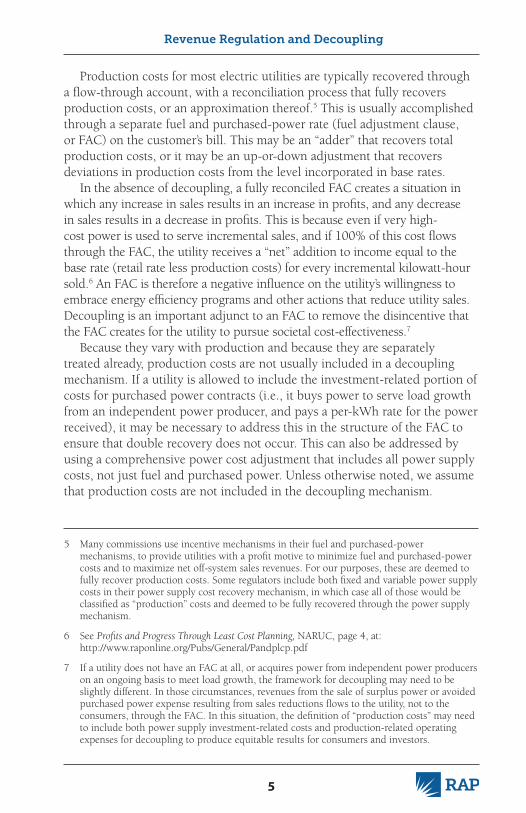
Production costs for most electric utilities are typically recovered through a flow-through account, with a reconciliation process that fully recovers production costs, or an approximation thereof.5 This is usually accomplished through a separate fuel and purchased-power rate (fuel adjustment clause, or FAC) on the customer’s bill. This may be an “adder” that recovers total production costs, or it may be an up-or-down adjustment that recovers deviations in production costs from the level incorporated in base rates.

In the absence of decoupling, a fully reconciled FAC creates a situation in which any increase in sales results in an increase in profits, and any decrease in sales results in a decrease in profits. This is because even if very high-cost power is used to serve incremental sales, and if 100% of this cost flows through the FAC, the utility receives a “net” addition to income equal to the base rate (retail rate less production costs) for every incremental kilowatt-hour sold.6 An FAC is therefore a negative influence on the utility’s willingness to embrace energy efficiency programs and other actions that reduce utility sales. Decoupling is an important adjunct to an FAC to remove the disincentive that the FAC creates for the utility to pursue societal cost-effectiveness.7

Because they vary with production and because they are separately treated already, production costs are not usually included in a decoupling mechanism. If a utility is allowed to include the investment-related portion of costs for purchased power contracts (i.e., it buys power to serve load growth from an independent power producer, and pays a per-kWh rate for the power received), it may be necessary to address this in the structure of the FAC to ensure that double recovery does not occur. This can also be addressed by using a comprehensive power cost adjustment that includes all power supply costs, not just fuel and purchased power. Unless otherwise noted, we assume that production costs are not included in the decoupling mechanism.

5 Many commissions use incentive mechanisms in their fuel and purchased-power mechanisms, to provide utilities with a profit motive to minimize fuel and purchased-power costs and to maximize net off-system sales revenues. For our purposes, these are deemed to fully recover production costs. Some regulators include both fixed and variable power supply costs in their power supply cost recovery mechanism, in which case all of those would be classified as “production” costs and deemed to be fully recovered through the power supply mechanism.

6 See Profits and Progress Through Least Cost Planning, NARUC, page 4, at: http://www.raponline.org/Pubs/General/Pandplcp.pdf

7 If a utility does not have an FAC at all, or acquires power from independent power producers on an ongoing basis to meet load growth, the framework for decoupling may need to be slightly different. In those circumstances, revenues from the sale of surplus power or avoided purchased power expense resulting from sales reductions flows to the utility, not to the consumers, through the FAC. In this situation, the definition of “production costs” may need to include both power supply investment-related costs and production-related operating expenses for decoupling to produce equitable results for consumers and investors.

6


3 .1 .1 .2 Non-Production CostsNon-production costs include all those that are not production costs — in

essence, everything that is related to the delivery of electricity (transmission, distribution, and retail services) to end users. This normally includes all non-production related O&M expenses, including depreciation and interest on debt. In many cases, the base rates also include the debt and equity service (i.e., the interest, return, and depreciation) on power supply investments, in which case the form of the FAC becomes important.

Statistically, a utility’s non-production costs do not vary much with consumption in the short run, but are more affected by changes in the numbers of customers served, inflation, productivity, and other factors.8 Of course, a utility with a large capital expenditure program, such as the deployment of smart grid technologies or significant rebuilds of aging systems, will experience a surge in costs that is unrelated to customer growth. Decoupling does not address this issue, which is better handled in the context of a rate case or infrastructure tracking mechanism.

Non-production costs are usually recovered through a combination of a cus-tomer charge,9 plus one or more volumetric (per kWh, per kW) rates. A utility may face the risk of not recovering some non-production costs if sales decline. Put another way, many of the costs do not vary with sales, so each dollar decline in sales flows straight to — and adversely affects — the bottom line.

3 .1 .2 ReturnFor our purposes, the utility’s “return” is the same as its net, after-tax profit,

or net income for common stock.10 When computing a revenue requirement for a rate case, this line item is derived by multiplying the utility’s net equity investment by its “allowed” rate of return on common equity. We have simplified this return in the illustration, but will address it in more detail in Section 10, Earnings Volatility Risks and Impacts on the Cost of Capital.

In a rate case, the return is a static expected value. In between rate cases,

8 Eto, Joseph, Steven Stoft, and Timothy Belden, The Theory and Practice of Decoupling, Lawrence Berkeley National Laboratory, January 1994. URL: http://eetd.lbl.gov/ea/EMS/reports/34555.pdf

9 In place of a customer charge, one may also find other monthly fixed charges, such as minimum purchase amounts, access fees, connection fees, or meter fees. For our purposes, these are all the same because they are not based on energy consumption, but, instead, are a function of the number of customers.

10 Regulatory commissions often calculate an “operating income” figure in the process of setting rates; this does not take account of the tax effects on the debt and equity components of the utility capital structure. Net income includes these effects.

11 Shirley, W., J. Lazar, and F. Weston, Revenue Decoupling: Standards and Criteria, A Report to the Minnesota Public Utilities Commission, Regulatory Assistance Project, 30 June 2008, Appendix B, p. 36.

http://eetd.lbl.gov/ea/EMS/reports/34555.pdf

http://eetd.lbl.gov/ea/EMS/reports/34555.pdf

7


realized returns are a function of actual revenues, actual investments, and actual expenses, all of which change between rate cases in response to many factors, including sales volumes, inflation, productivity, and many others.

As a share of revenues in a rate case revenue requirement calculation, the return on equity to shareholders may be as small as 5%-10%. As a result, small percentage changes in total non-production revenues (all of which largely affect return and taxes) can generate large percentage changes in net profits.11

3 .1 .3 TaxesIn a rate case, the amount of taxes a utility would pay on its allowed

return is added to the revenue requirement.In between rate cases, taxes buffer the impact on the utility’s shareholders

of any deviations of realized returns from expected returns. When realized returns rise, some portion is lost to taxes, so shareholders do not garner gains one-for-one with changes in net revenues. Conversely, if revenues fall, so do taxes. As a result, investors do not suffer the entire loss. If the tax rate is 33%, then one third of every increase or decrease in pre-tax profits will be absorbed by taxes.

From a customer perspective, there is no buffering effect from taxes. To the contrary, customers pay all additional revenues and enjoy all savings, dollar for dollar.

3 .1 .4 Between Rate CasesWith traditional regulation, while the

determination of the revenue requirement at the time of the rate case decision is meticulous, the utility will almost certainly never collect precisely the allowed amount of revenue, experience the associated assumed levels of expenses or unit sales, or achieve the expected profits. The revenue requirement is only used as input to the price determination. Once prices are set, realized revenues and profits will be a function of actual sales and expenses and will have only a rough relationship with the rate case allowed revenues or returns.

Put another way, traditional regulation fixes the price between rate cases and lets revenues float up or down with actual sales. At this point, the rate case formulae no longer hold sway. Instead, two different mathematical realities operate:

Formula 3: Revenues ActuAl = Units Sold Actual X PriceFormula 4: Profit ActuAl = (Revenues – Expenses – Taxes) ActuAll

These two formulae reveal the methods by which the utility can increase its profits. One approach is to reduce expenses. Providing a heightened

Traditional regulation fixes

the price between rate cases and

lets revenues float up or down with

actual sales.

8


incentive to operate efficiently is sound. However, there is a floor below which expenses simply cannot be reduced without adversely affecting the level of service, and to ensure that utilities cut fat, but not bone, some regulators have established service quality indices that penalize utilities that achieve lower-than-expected customer service quality. The easier approach is to increase the Units Sold, as this will increase revenues and therefore profits.12 This is the heart of the throughput incentive that utilities traditionally face – and this is where decoupling comes in.

3.2 How Decoupling Works

There are a variety of different approaches to decoupling, all of which share a common goal of ensuring the recovery of a defined amount of revenue, independent of changes in sales volumes during that period. Some are computed on a revenue-per-customer basis, while others use an attrition adjustment (typically annual) to set the allowed revenue. Some operate on an annual accrual basis, while others operate on a current basis in each billing cycle. Table 2 categorizes these and provides an example of each approach; a greater discussion of these approaches is contained in the appendix.

Table 2

12 This is because, as noted earlier, the utility faces virtually no changes in its non-production costs as its sales change. This means that marginal increases in sales will have a large and posi-tive impact on the bottom line, just as marginal reductions in sales will have the opposite effect.

Decoupling Methodology

Accrual Revenue Per Customer

Current Revenue Per Customer

Accrual Attrition

Distribution-Only

Key Elements

Allowed revenue computed on an RPC basis; one rate adjustment per year

Allowed revenue computed on an RPC basis; rates adjusted each billing cycle to avoid deferrals

Allowed revenue determined in periodic general rate cases; changes to this based on specified factors determined in annual attrition reviews; rates adjusted once a year

Only distribution costs included in the mechanism; all power costs (fixed and variable) recovered outside the decoupling mechanism

Example of Application

Utah, Questar

Oregon, Northwest Natural Gas Company;DC: Pepco

California, PG&E and SCE Hawaii, Hawaiian Electric

Massachusetts, NGridMaryland, BG&EWashington (PSE, 1990-95)

9


3 .2 .1 In the Rate Case (It’s the same)With decoupling there is no change in the rate case methodology, except

perhaps for the migration of some cost items into or out of the production cost recovery mechanism.13 Initial prices are still set by the regulator, based on a computed revenue requirement.

Formula 1: Revenue Requirement = (Expenses + Return + Taxes) test Period

Formula 5: Price end of rAte cAse = Revenue Requirement ÷ Units Sold test Period

3 .2 .2 Between Rate Cases (It’s different)With decoupling, the price computed

in the rate case is only relevant as a reference or beginning point. In fact, the rate case prices may never actually be charged to customers. Instead, under “current” decoupling (described below), prices can be adjusted immediately, based on actual sales levels, to keep revenues at their allowed level. Rather than holding prices constant between rate cases as traditional regulation would do, decoupling adjusts prices periodically, even as frequently as each billing cycle, to reflect differences between units sold test Period and units sold ActuAl, as necessary to collect revenues Allowed. This is accomplished by applying the following formulae:

Formula 6: Price Post rAte cAse = Revenues Allowed ÷ Units Sold ActuAl

Formula 7: Revenues ActuAl = Revenues Allowed

Formula 4: Profits ActuAl = (Revenues – Expenses – Taxes) ActuAl

Table 3 gives an example of the calculations.

13 Examples of costs that are sometimes recovered on an actual cost basis include nuclear decom-missioning (which rises according to a sinking fund schedule), energy conservation program expenses, and infrastructure trackers for non-revenue-generating refurbishments. Where a utility does not have an FAC or purchases power from independent power producers to meet load growth, it may be necessary to include all power supply costs, fixed and variable, in the definition of “production costs.”

There are two distinct components of decoupling

which are embedded in the decoupling formulae:

determination of the utility’s allowed revenues and determination of the prices necessary to collect those allowed revenues.

10


There are two distinct actions embedded in the decoupling formulae: determination of the utility’s allowed revenues and determination of the prices necessary to collect those allowed revenues. The former can involve a variety of methods, ranging from simply setting allowed revenues at the amount found in the last rate case to varying revenues over time to reflect non-sales-related influences on costs and revenues, as discussed in Section 5, Revenue Functions. The latter is merely the calculation which sets the prices that, given sales levels (i.e., billing determinants), will generate the allowed revenue.

Put another way, while traditional regulation sets prices, then lets revenues float up or down with consumption, decoupling sets revenues, then lets prices float down or up with consumption. This price recalculation is done repeatedly – either with each billing cycle or on some other periodic basis (e.g., annual), through the use of a deferral balancing and reconciliation account.14

There are two separate elements in play in the price-setting component of decoupling. The first is that prices are allowed to change between rates, based on deviations in sales from the test period assumptions. The second is the frequency of those changes. We discuss the frequency idea in greater detail in Section 8, Application of Decoupling: Current vs. Accrual Methods.

Expenses . . . . . . . . . . . . . . . . . $100,000,000

Net Equity Investment . . . . . . . $100,000,000

Allowed Rate of Return . . . . . . . . . . . 10 .00%

Allowed Return . . . . . . . . . . . . . $10,000,000

Taxes (35% tax rate) . . . . . . . . . $15,384,615

Total Revenue Requirement . . . $115,384,615

Price Calculation

Revenue Requirement . . . . . . . $115,384,615

Actual Sales (kWh) . . . . . . . . . . 990,000,000

Decoupling Price ($/kWh) . . . . . . . . . $0 .1166

Decoupling Adjustment ($/kWh) . . . . $0 .0012

Decoupling Example:Revenue Requirement Calculation

Table 3

14 There are, however, good reasons to seek to limit the magnitude of deviations from the reference price. For example, many decoupling mechanisms allow a maximum 3% change in prices in any year, deferring larger variations for future treatment by the regulator. Significant variability in price may threaten public acceptance of decoupling and the broader policy objectives it serves. Policymakers should be careful to design decoupling regimes with this consideration in mind.

While traditional regulation sets prices, then

lets revenues float up or down with consumption, decoupling sets revenues, then lets prices float down or up with consumption.

11


4 Full, Partial, and Limited Decoupling

We use a specialized vocabulary to differentiate various approaches to decoupling.

4.1 Full Decoupling

Decoupling in its essential, fullest form insulates a utility’s revenue collections from any deviation of actual sales from expected sales. The cause of the deviation — e.g., increased investment in energy efficiency, weather variations, changes in economic activity — does not matter. Any and all deviations will result in an adjustment (“true-up”) of collected utility revenues with allowed revenues. The focus here is delivering revenue to match the revenue requirement established in the last rate case.

Full decoupling can be likened to the setting of a budget. Through currently used rate-case methods, a utility’s revenue requirement — i.e., the total revenues it will need in a period (typically, a year) to provide safe, adequate, and reliable service — is determined. The utility then knows exactly how much money it will be allowed to collect, no more, no less. Its profitability will be determined by how well it operates within that budget. Actual sales levels will not, however, have any impact on the budget.15

The most common form of full decoupling is revenue-per-customer decoupling, which is more fully explained with other forms of decoupling in the next section. The California approach, wherein a revenue requirement is fixed in a rate case and incremental (or decremental) adjustments to it are determined in periodic “attrition” cases, is also a form of full decoupling. Tracking mechanisms, designed to generate a set amount of revenue to

15 This is the simplest form of full decoupling. As described in the next section, most decoupling mechanisms actually allow for revenues to vary as factors other than sales vary. The reasoning is that, though in the long run utility costs are a function of demand for the service they provide, in the short run (i.e., the rate-case horizon) costs vary more closely with other causes, primarily changes in the numbers of customers.

Full decoupling can be likened to the setting of a

budget.

12


cover specific costs (independently of base rates and the underlying cost of service) are not incompatible with full decoupling. They would be reflected in separate tariff surcharges or surcredits.

Full decoupling renders a utility indifferent to changes in sales, regardless of cause. It eliminates the “throughput” incentive. The utility’s revenues are no longer a function of sales, and its profits cannot be harmed or enhanced by changes in sales. Only changes in expenses will then affect profits.

Decoupling eliminates a strong disincentive to invest in energy efficiency. By itself, however, decoupling does not provide the utility with a positive incentive to invest in energy efficiency or other customer-sited resources, but it does remove the utility’s natural antagonism to such resources due to their adverse impact on short-run profits. Assuming that management has a limited ability to influence costs and behavior, this allows concentration of that effort on cost reductions, rather than sales enhancements.

4.2 Partial Decoupling

Partial decoupling insulates only a portion of the utility’s revenue collections from deviations of actual from expected sales. Any variation in sales results in a partial true-up of utility revenues (e.g., 50%, or 90%, of the revenue shortfall is recovered).

One creative application of partial decoupling was the combination conservation incentive/decoupling mechanism for Avista Utilities in Washington. The utility was allowed to recover a percentage of its lost distribution margins from sales declines in proportion to its percentage achievement of a Commission-approved conservation target. If it achieved the full conservation target, it was allowed to recover all of its lost margins, but if it fell short, it was allowed only partial recovery.16 This proved a powerful incentive to fully achieve the conservation goal.

4.3 Limited Decoupling

Under limited decoupling only specified causes of variations in sales result in decoupling adjustments. For example:

• Onlyvariationsduetoweatheraresubjecttothetrue-up(i.e.,actualyear revenues [sales] are adjusted for their deviation from weather-normalized revenues). This is simply a weather normalization adjustment clause. Other impacts on sales would be allowed to affect revenue collections. Successful implementation of energy efficiency programs would, in this context, result in reductions in sales and

16 Washington Utilities and Transportation Commission, Docket UG-060518, 2007. The recovery was capped at 90%.

13


revenues from which the utility would not be insulated — that is, all else being equal, energy efficiency would adversely affect the company’s bottom line. Weather-only adjustment mechanisms have been implemented for several natural gas distribution companies.

• Lost-marginmechanisms,whichrecoveronlythelostdistributionmargin related to utility-operated energy efficiency programs, have been implemented for several utilities. These generally provide a removal of the disincentive for utilities to operate efficiency programs, but may create perverse incentives for utilities to discourage customer-initiated efficiency measures or improvements in codes and standards that cause sales attrition, because these are not compensated.

• Reducedusagebyexistingcustomersmaybe“decoupled,”whereasnew customers are not included in the mechanism, on the theory that the utility is more able to influence, through utility programs, the usage of existing customers who were a part of the rate-case determination of a test year revenue requirement.

• Variationsduetosomeorallotherfactors(e.g.,economy,end-useefficiency) except weather are included in the true-up. In this instance, the utility and, necessarily, the customers still bear the revenue risks associated with changes in weather. And, lastly,

• Somecombinationoftheabove.Limited decoupling requires the application of more complex

mathematical calculations than either full or partial decoupling, and these calculations depend in part on data whose reliability is sometimes vigorously debated. But more important than this is the fundamental question that the choice of approaches to decoupling asks: how are risks borne by utilities and consumers under decoupling, as opposed to traditional regulation? What value derives from removing sales as a motivator for utility management? What value derives from creating a revenue function that more accurately collects revenue to match actual costs over time? What are the expected benefits of decoupling, and what, if anything, will society be giving up when it replaces traditional price-based regulation with revenue-based regulation?

Limited decoupling does not fully eliminate the throughput incentive. The utility’s revenues (and profits, therefore) are still to some degree dependent on sales. So long as it retains a measure of sales risk, the achievement of public policy goals in end-use efficiency and customer-sited resources, environmental protection, and the least-cost provision of service will be inhibited.17

17 “Limited decoupling” is synonymous with “net lost revenue adjustments.” “Net lost revenue adjustments” is the term of art that describes earlier methods of compensating a utility for the revenue to cover non-production costs that it would have collected had specified sales-reducing events or actions (e.g., cooler-than-expected summer weather, or government-mandated end-use energy investments) not occurred.

14


5 Revenue Functions

One of the collateral benefits of decoupling is the potential for reducing the frequency of rate cases. In its simplest form, a decoupling mechanism maintains revenues at a constant level between rate cases. However, this would inevitably put increasing

downward pressure on earnings due to general net growth in the utility’s cost structure as new customers are added and operating expenses are driven by inflation, to the extent these are not offset by depreciation, productivity gains, and, in certain cases, cost decreases.

To avoid this problem, the allowed (or “target”) revenue a utility can collect in any post-rate-case period can be adjusted relative to the rate-case revenue requirement. Most decoupling mechanisms currently in effect make use of one or more revenue functions to set allowed revenues between rate cases, and we describe the four standard ones here: (1) adjusting for inflation and productivity; (2) accounting for changes in numbers of customers; (3) dealing with attrition in separate cases; and (4) the application of a “K” factor to modify revenue levels over time. There may be others that are, in particular circumstances, also appropriate.

5.1 Inflation Minus Productivity

Before development of the current array of decoupling options, a number of jurisdictions used what has been called “performance-based regulation” (PBR) — relying on a price-cap methodology, instead of decoupling’s revenue-based approach. These plans, first developed for telecommunications providers, often included a price adjuster under which the affected (usually non-production) costs of the utility were assumed to grow through the net effects of inflation (a positive value) and increased productivity (a negative

18 Under normal economic conditions, inflation will be a positive value and productivity a negative value, but there can be circumstances that violate this presumption — an extended period of deflation, for instance. In fact, when Great Britain’s state-owned electric transmission and distribution companies were privatized in the late 1980s, their prices were regulated under PBR formulas that included positive productivity adjustments. “[Positive] X (that is, an apparent allowance for annual rates of productivity decreases of X percent) factors were chosen in order to provide the industry with sufficient future cash flow in part to meet projected future investment needs and also to increase the attractiveness of the companies to the investment

15


value).18 Prices were allowed to grow at the rate of inflation, less productivity, in an effort to track these expected changes in the utility’s cost of service. In some cases, other factors (often called “Z” factors) were added to the formulae to represent other explicit or implicit cost drivers. For example, if a union contract had a known inflationary factor, this might be used in lieu of a general inflation index, but only for union labor expenses.

This adjustment is being used in revenue-decoupling regulation, too, to determine a revenue path between rate cases. Rather than applying this adjustment to prices, it is applied to the allowed revenue between rates cases.19 This approach is used in California, with annual “attrition” cases that consider other changes since the last general rate case, then add (or subtract) these from the revenue requirement determined in the rate case.

With the inflation and productivity factors in hand, the allowed revenue amount can be adjusted periodically. In practice, this adjustment has usually been done through an annual administrative filing and review. In theory, however, there is no practical reason these adjustments could not be made on a current basis, perhaps with each billing cycle.20 In application, the net growth in revenue requirement is usually spread evenly across all customers and all customer classes.

The inflation-minus-productivity approach does not remove all uncertainty from price changes, because the actual inflation rate used to derive allowed revenues (and, therefore, reference prices) will vary over time.

community during their upcoming public auction. The initial regulatory timeframe was set at the fiscal year 1990/1995 time period.” See http://actrav.itcilo.org/actrav-english/telearn/global/ilo/frame/elect2.htm. (Note that this adjustment is actually referred to as “negative productivity,” since it indicates a reduction, rather than an increase, in productivity. Mathematically, it’s denoted as the negative of a negative, and so for simplicity’s sake we’ve described it as positive here.)

19 Under this approach, a government-published (or other accepted “third party” source), broad-based inflation index is used. The productivity factor, which serves to offset inflation, is also an administratively determined or, in some cases, a stakeholder agreed-upon value. It should not, however, be calculated as a function of the particular company’s own productivity achievements. Doing so would reward a poorly performing company with an overall revenue adjustment (inflation-minus-productivity factor) that is too high (and which does not give it strong enough incentives to control costs) and would punish a highly performing company with a factor that reduces the gains it would otherwise achieve, in effect holding it to a more stringent standard than other companies face.

20 See also Current vs. Accrual Methods, below, for more on the implications of using accrual methodologies for decoupling versus using a current system. It goes without saying, of course, that price changes of this sort can only be effected through a simple, regular ministerial process, if the adjustment factors on which they are based are transparent, unambiguous, and factual in nature (e.g., customer count). If, however, the adjustment is driven by changes that are within management’s discretionary — say, capital budget — then a more detailed review may be required to assure that prudent decisions are underlying the revenue adjustments.

http://actrav.itcilo.org/actrav-english/telearn/global/ilo/frame/elect2.htm

http://actrav.itcilo.org/actrav-english/telearn/global/ilo/frame/elect2.htm

16


5.2 Revenue-per-Customer (RPC) Decoupling

As noted earlier, analysis has shown that, in the time between rate cases, changes in a utility’s underlying costs vary more directly with changes in the number of customers served than they do with other factors such as sales, although the correlation on a total expense basis to any of these is relatively weak. When examining only non-production costs, however, the correlations are much stronger, especially for the number of customers.

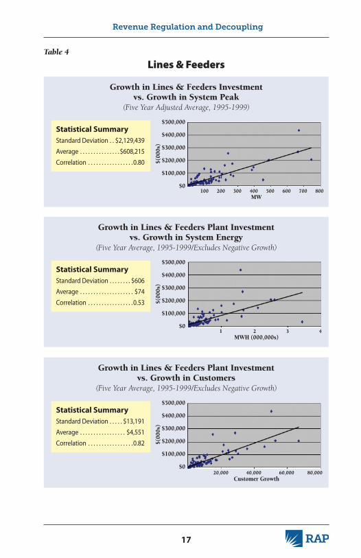
In 2001, we previously studied the relationships between drivers such as system peak, total energy, and number of customers to investments in distribution facilities.21

RAP prepared studies for correlations between investments in transformers and substations versus lines and feeders as they relate to growth in customers served, system peak, and total energy sales. The data indicate that customer count is somewhat more closely correlated with growth in non-production costs, stronger than either growth in system peak or growth in energy sales. These data support using the number of customers served as the driver for computing allowed revenues between rate cases, particularly in areas where customer growth has been relatively stable and is expected to continue. The revenue-per-customer, or RPC method, may not be appropriate in areas with stagnant economies or volatile spurts of growth, or where new customers are significantly different in usage patterns than existing customers, but in these situations, the attrition method may still work well.

The RPC value is derived through an added “last” step in the rate case determination. It is computed by taking the test period revenues associated with each volumetric price charged, and dividing that value by the end-of-test period number of customers who are charged that volumetric price. This calculation must be made for each rate class, for each volumetric price, and for each applicable billing period (most likely a billing cycle):

Formula 8: Revenue per Customer test Period = Revenue Requirement test Period ÷ No . of Customers test Period

With this revenue-per-customer number, allowed revenues can be adjusted periodically to reflect changes in numbers of customers. In any

The data indicate that customer growth is closely

correlated to growth of non-production costs.

21 See Distributed Resource Policy Series: Distribution System Cost Methodologies for Distributed Generation available at http://www.raponline.org/docs/RAP_Shirley_DistributionCostMethodologiesforDistributedGeneration_2001_09.pdf and the accompanying Appendices at: http://www.raponline.org/docs/RAP_Shirley_DistributionCostMethodologiesforDistributedGenerationAppx_2001_09.pdf

http://www.raponline.org/docs/RAP_Shirley_DistributionCostMethodologiesforDistributedGeneration_2001_09.pdf

http://www.raponline.org/docs/RAP_Shirley_DistributionCostMethodologiesforDistributedGeneration_2001_09.pdf

http://www.raponline.org/docs/RAP_Shirley_DistributionCostMethodologiesforDistributedGenerationAppx_2001_09.pdf

http://www.raponline.org/docs/RAP_Shirley_DistributionCostMethodologiesforDistributedGenerationAppx_2001_09.pdf

17


Statistical SummaryStandard Deviation . . $2,129,439Average . . . . . . . . . . . . . . .$608,215Correlation . . . . . . . . . . . . . . . . .0 .80

Statistical SummaryStandard Deviation . . . . . . . . $606Average . . . . . . . . . . . . . . . . . . . . $74Correlation . . . . . . . . . . . . . . . . .0 .53

Statistical SummaryStandard Deviation . . . . . $13,191Average . . . . . . . . . . . . . . . . . $4,551Correlation . . . . . . . . . . . . . . . . .0 .82

$500,000

$400,000

$300,000

$200,000

$100,000

$0

$500,000

$400,000

$300,000

$200,000

$100,000

$0

$500,000

$400,000

$300,000

$200,000

$100,000

$0

Growth in Lines & Feeders Investment vs . Growth in System Peak

(Five Year Adjusted Average, 1995-1999)

Growth in Lines & Feeders Plant Investment vs . Growth in System Energy

(Five Year Average, 1995-1999/Excludes Negative Growth)

Growth in Lines & Feeders Plant Investment vs . Growth in Customers

(Five Year Average, 1995-1999/Excludes Negative Growth)

100 200 300 400 500 600 700 800MW

1 2 3 4MWH (000,000s)

20,000 40,000 60,000 80,000Customer Growth

$(00

0s)

$(00

0s)

$(00

0s)

Table 4

Lines & Feeders

18


post-rate-case period, the allowed revenues for energy and demand charges are calculated by multiplying the actual number of customers served by the RPC value for the corresponding billing period. The decoupling adjustment is then calculated in the manner detailed in the earlier sections.

Formula 9: Revenues Allowed = Revenue per Customer test Period X No . of Customers ActuAl

Formula 10: Price ActuAl = Revenues Allowed ÷ Units Sold ActuAl

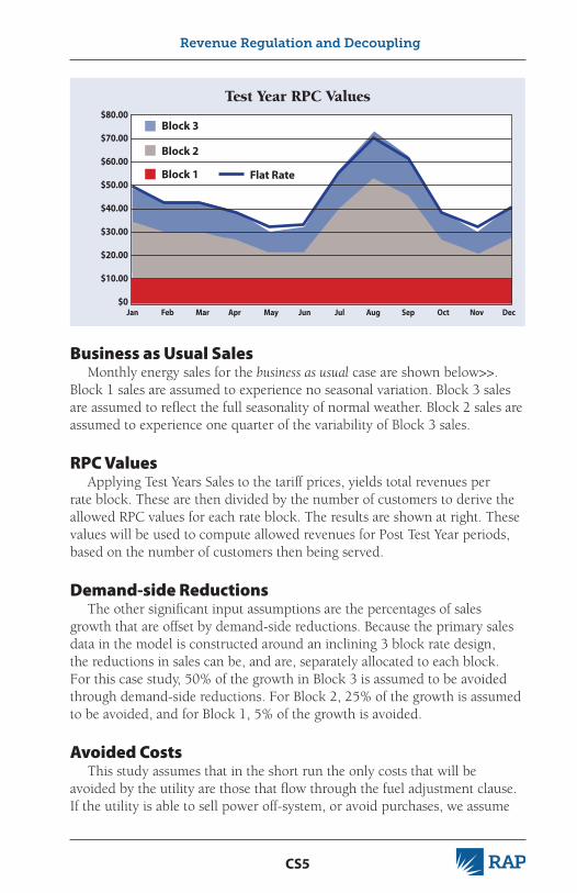
The table below demonstrates the RPC calculations for three billing periods for a sample small commercial rate class. In this example, the billing periods are assumed to be monthly. Note that the revenues per customer are different in each month, because of the seasonality of consumption in the test period.22

By calculating the energy and demand revenues per customer for each

Table 5

Deriving the Revenue per Customer Values

Small Commercial Class ExampleTest Period Values

Billing Period 1 2 3

Number of Test Period Customers 142,591 142,769 142,947 Customer Charge $25.00 $25.00 $25.00Total Customer Charge Revenues $3,564,775 $3,569,225 $3,573,675

Energy Revenue per CustomerEnergy Sales (kWh) 181,238,883 189,304,436 170,240,013 Rate Case Price $0.165 $0.165 $0.165Total Energy Sales Revenues $29,904,416 $31,235,232 $28,089,602Energy Revenue per Customer $209.72 $218.78 $196.50

Demand Revenue per CustomerDemand Sales (kW) 1,189,355 1,165,396 1,148,975 Rate Case Price $4.4600 $4.4600 $4.4600Total Demand Sales Revenues $5,304,523 $5,197,667 $5,124,429Demand Revenue per Customer $37.20 $36.41 $35.85

22 Most utilities typically have 22 or 23 billing cycles per month. For simplicity, we have assumed here that all customers in a month are billed in the same billing cycle (one per month). In the future, with new “smart” metering and communication platforms, a single billing cycle per month, for all customers, may be possible.

19


billing period, normal seasonal variations in consumption are automatically captured. This causes revenue collection to match the underlying seasonal consumption patterns of the customers.

Some decoupling schemes exclude very large industrial customers. Because the rates for these customers are often determined by contractual requirements and specified payments designed to cover utility non-production costs, there may be little or no utility throughput incentive opportunity relating to these customers anyway. Also, in many utilities, this class of customers may consist of only a small number of large and unique (in load-shape terms) customers, so that a “class” approach is not apt.

In cases in which new customers (that is, those who joined the system during the term of the decoupling plan) have significantly different consumption patterns (and, therefore, revenue contributions to the utility) than existing customers, regulators may want to modify the decoupling formula to account for the difference. This can be accomplished by using different RPC values for new customers and existing customers. The nature of this issue and methodologies for addressing it are discussed in Section 6, Application of RPC Decoupling: New vs. Existing Customers.

5.3 Attrition Adjustment Decoupling

Some jurisdictions take a different approach to decoupling. They set base rates in a periodic major rate case, then conduct annual abbreviated reviews to determine whether there are particular changes in costs that merit a change in rates. In such instances, the regulators adjust rate base and operating expenses only for known and measurable changes to utility costs and revenues since the rate case, and adjust for them through a small increment or decrement to the base rates (called “attrition adjustments”). The regulators normally do not consider more controversial issues such as new power plant additions or the creation of new classes of customers, which are reserved for general rate cases.

In attrition decoupling, the utility’s allowed revenue requirement is the amount allowed in the first year after the rate case, plus the addition (or reduction) that results from the attrition review. Every few years, a new general rate case is convened to re-establish a cost-based revenue requirement considering all factors.

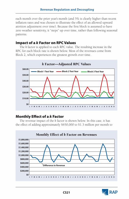
5.4 K Factor

The K factor is an adjustment used to increase or decrease overall growth in revenues between rate cases.

In its simplest application, the K factor can be used in lieu of either the

20


inflation-minus-productivity method or the RPC method; it could be, for example, a specified percentage per year. Although one could vary the K factor itself over time, in this context the most likely application would simply set an annual between-rate-case growth rate for revenues, resulting in a steady change (probably an increase) in year-to-year allowed revenues for each period between rate cases. Such an approach has a high degree of certainty, but runs the risk of being disassociated from, and therefore out of sync with, measurable drivers of a utility’s cost of service. All of the data used in a rate case change over time, and the elements making up the K factor are no different. The K factor therefore may become obsolete within a few years, providing another reason why periodic general rate cases should be required by regulators under decoupling (and, arguably, under traditional regulation as well).

An alternative approach is to use the K factor as an adjustment to the RPC allowed revenue determination. Here, the K factor growth rate (positive or negative) would be applied to the RPC values, rather than to the allowed revenue value itself. This approach would be useful when an additional revenue requirement is anticipated due to identifiable increases in revenues from capital expenditures or operating expenses, or because of some underlying trend in the RPC values. An example would be a utility with a distribution system upgrade program driven by reliability concerns, where the investment is not generating new revenue. It may also be used as an incentive for the utility to make specific productivity gains, in which case the K factor would be a negative value causing revenues to be slightly lower than they otherwise would have been.

In any case, allowed revenues would still be primarily driven by the number of customers served, but the revenue total would be driven up or down by the K factor adjustment.

Formula 11: Revenue Per Customer Allowed = Revenue Per Customer test Period * K

Formula 12: Revenues Allowed = Revenue Per Customer Allowed X No . of Customers ActuAl

Formula 10: Price ActuAl = Revenues Allowed ÷ Units Sold ActuAl

A “successful” revenue function would be one that keeps the utility’s

actual revenue collection as close as possible to

its actual cost of service throughout the period

between rate cases.

21


5.5 Need for Periodic Rate Cases

It is useful to have periodic rate cases in which all costs, expenses, investments, programs, policies, and tariff designs can be examined. Many regulators have required general rate cases every three to five years as part of decoupling (or set expiration dates for the decoupling mechanism). Another approach would be a built-in decline in the allowed revenue (or RPC) after three to five years. This would allow the utility to avoid a new general rate case (in which all of the utility’s costs would be examined), but only if it reduced customer bills. This leaves the utility with the option to continue to retain a portion of expense containment savings motivated by decoupling (see Formula 4) without a rate case, if it can reduce costs sufficiently to give consumers a measurable benefit.

5.6 Judging the Success of a Revenue Function

One of the shortcomings of traditional utility pricing approaches is that a utility’s actual revenue collection can be significantly higher or lower than its actual cost of providing service. The different revenue functions that can be applied with decoupling offer means of keeping the utility’s revenue collections much closer to its actual cost of service over time. This should result in smaller rate case revenue deficiencies or excesses, lessening their associated potential for “rate shock.”

A “successful” revenue function would be one that keeps the utility’s actual revenue collection as close as possible to its actual cost of service throughout the period between rate cases. Indeed, the theoretically ideal result, by this standard, would be to have a zero revenue deficiency or excess in the next rate case and at most points in between, meaning that rates had tracked costs perfectly over time.

Of course, when judging the revenue function on this basis, one should disregard special circumstances that may cause a significant revenue deficiency, such as large additions to the utility’s plant-in-service accounts (e.g., the addition of a new transmission line, the installation of an expensive new management information system, or the deployment of smart-grid advanced metering infrastructure).

22


6 Application of RPC Decoupling: New vs. Existing Customers

As much as half of the change in average usage per customer over time may be explained by differences between existing and new customers. Where new customers, on average, have significantly different usage than existing customers, their addition to the

decoupling mechanism can result in small cross-subsidies.New customers may be significantly different from existing customers.

For example, new building codes and appliance standards may mean that new customers are fundamentally more efficient. Typical new homes may be larger or smaller than the average of existing homes (or may reflect a different mix of single-family and multi-family construction). If urban areas are becoming more densely populated, it may mean that new customers are closer together, and thus there is a smaller distribution system investment per customer. If line extension policies require new customers to pay a larger share of distribution system expansion costs than existing customers did, the investment added to the utility rate base per customer may be smaller for new customers. If the regulator is concerned that there may be meaningful differences between new and existing customers, it can require the utility to perform a detailed analysis of usage characteristics (quantity, seasonality, time-of-day) for each cohort of customers connected to the system.

As illustrated in Table 6, new customers, on average, use 450 kWh in a billing period, but the rate case-derived RPC for existing customers is 500 kWh, application of the test year RPC values to new customers has the effect of causing old customers to bear the revenue burden associated with the 50 kWh not needed or used by new customers. This is because the allowed revenue is increased by an amount associated with 500 kWh of consumption, whereas the actual contribution to revenues from the new customers is only the amount associated with 450 kWh.

Where new customers, on average, have

significantly different usage than existing

customers, their addition to the decoupling

mechanism can result in small crosssubsidies

23


To correct for this, a separate RPC value can be calculated for new customers — in our example, the amount for them would be $45.00. As shown in Table 7, the RPC allowed revenues would not be increased from $10,000,000 to $10,025,000. Instead, the increase would be equal to only $22,500.

This results in collection of an average of $50.00 from existing customers and $45.00 from new customers, thus reflecting the overall lower usage of new customers. On a total basis, the average revenues per customer are equal to $49.76. Accounting for these differences affects the allowed revenue to assure no over- or under-recovery, while differences in bills for these two types of customers are automatically reflected in their respective units of consumption applied to the decoupled price.

Table 6

Table 7

Number of Customers 200,000 10,000 210,000Revenue per Customer $50.00 $45.00Allowed Revenues $10,000,000 $450,000 $10,450,000Average Unit Sales 500 450Decoupled Price $0.100000 $0.100000Collected Revenues $10,000,000 $450,000 $10,450,000Average Customer Contribution $50.00 $45.00 $49.76

Number of Customers 200,000 10,000 210,000Revenue per Customer $50.00 $50.00Allowed Revenues $10,000,000 $500,000 $10,500,000Average Unit Sales 500 450Decoupled Price $0.100478 $0.100478Collected Revenues $10,047,847 $452,153 $10,500,000Average Customer Contribution $50.24 $45.22 $50.00

Single RPC for Existing and New Customers

Separate RPC for Existing and New Customers

Existing Customers

Existing Customers

New Customers

New Customers

Total

Total

24


7 Rate Design Issues Associated With Decoupling

As it does with respect to increased investment in end-use energy efficiency itself, decoupling should also remove traditional utility objections to electric and natural gas rate designs that encourage conservation, voluntary curtailment, and peak load management.

For example, assuming average usage of 500 kWh/month, the two following rate designs produce the same amount of revenue, but the volumetric rate provides a much stronger price signal for consumers to pursue energy efficiency:

Table 8

Customer Charge $25.00 $5.00

Usage Charge $0.10 $0.14

Total Bill for 500 kWh average usage $75.00 $75.00

High vs . Low Customer Charges

Rate Element High Customer Low Customer

Under volumetric pricing without decoupling, utilities have a significant portion of their revenue requirement for rate base and O&M expenses associated with throughput. In addition, those with fully reconciled fuel and purchased-power adjustment mechanisms completely recover the high cost of augmenting power supply during peak periods when expensive power resources are used, so even increased peak-period sales generate a distribution sales margin.23 A reduction of throughput will likely reduce

23 See Subsection 3.1.1.1 above, and Moskovitz, Profits and Progress Through Least Cost Planning, 1990, at pp. 3-5. Fuel adjustment mechanisms are the antithesis of energy efficiency mechanisms. They guarantee that any additional sale, no matter how expensive to serve, adds to profit, and any foregone sale diminishes profitability. This is because the clauses ensure that the marginal fuel or purchase cost of incremental sales will be fully recovered, so that the non-production cost component of base rates will always contribute to the bottom line (by either increasing profits or reducing losses). www.raponline.org/Pubs/General/Pandplcp.pdf .

25


revenues at a greater rate than it will produce savings in short-run costs, simply because most distribution, billing, and administrative costs are relatively fixed in the short run.

Conversely, with decoupling, the utility no longer experiences a net revenue decrease when sales decline, and will therefore be more willing to embrace rate designs that encourage customers to use less electricity and gas. This can be achieved through energy efficiency investment (with or without utility assistance), through energy management practices (turning out lights, managing thermostats), or through voluntary curtailment.

Currently, the best examples of this are the natural gas and electric rate designs used by California electricity and natural gas utilities, where decoupling has been in place for many years. The residential rates applicable to most customers of Pacific Gas and Electric (PG&E), typical of those of all gas utilities and at least the investor-owned electric utilities in the state, are shown in Table 9. Both the gas and electric rates are set up with a “baseline” allocation, which is set for each housing type and climate zone. Neither rate has a customer charge, although there is a minimum monthly charge for service. If usage in a month falls below the amount covered by the minimum bill, the minimum still applies.

Table 9

Table 10

Minimum Monthly Charge ~$3.00Base Rate per therm $1.45131 $1.68248Multi-Family Discount (per unit per day) $0.01770 $0.17700Low-income Discount (per therm) $0.29026 $0.33650Mobile Home Park Discount (per unit per day) $0.35600 $0.35600

Minimum monthly Charge ~$3.50 ~$4.45Baseline Quantities $0.83160 $0.11559101%-130% of Baseline $0.09563 $0.13142131%-200% of Baseline $0.09563 $0.22580201%-300% of Baseline $0.09563 $0.31304over 300% of Baseline $0.09563 $0.35876

PG&E Natural Gas Rate at May 1, 2008

PG&E Natural Gas Rate at May 1, 2008

Rate Element

Rate Element

Baseline Quantities

Low Income

Excess Quantities

All OtherCustomers

26


7.1 Revenue Stability Is Important to Utilities

Clearly these rate designs produce a great deal of revenue volatility for the utility. Without decoupling, the utility could face extreme variations in net income from year to year. However, with decoupling, this type of rate design produces very stable earnings. The earnings per share for PG&E (the utility) for the past three years (since decoupling was restored after the termination of the California deregulation experiment) have been $1.01 billion, $971 million, and $918 million. This stability was achieved despite a $1.4 billion increase in operating expenses, mostly the cost of electricity, during this period.

The revenue stability needs of the company can conflict with principles of cost-causation as they relate to pricing. Utilities are interested in revenue stability, so that they have net income that can predictably provide a fair rate of return to investors, regardless of weather conditions, business cycles, or the energy conservation efforts of consumers. Cost-of-service considerations, however, can produce a very different result. To the extent that utility fixed costs are associated with peak demand (peaking resources, transmission capacity, natural gas storage, and liquefied natural gas (LNG) facilities) and those capacity costs are allocated exclusively to increased use in winter and summer months, the cost to consumers of incremental usage is dramatically higher than the cost of base usage.

A steeply inverted block rate design, such as those used by PG&E, correctly associates the cost of seldom-used capacity with the (infrequent) usage for which that capacity exists. Although this is arguably fair, doing so can result in serious revenue stability problems for the utility. Decoupling is one way to provide revenue stability for the utility, without introducing rate design elements such as high fixed monthly charges, in the form of a Straight Fixed/Variable rate design, that remove the appropriate price signals to consumers.

7.2 Bill Stability Is Important to Consumers

Customers also have an interest in bill stability, because in extremely cold winters or hot summers, their bills can quickly become unmanageable. Absent decoupling, rates such as those used in California, while accurately conveying the real cost of seldom-used capacity, accentuate bill volatility. In a hot summer or cold winter, consumer bills can soar as their end-block usage increases. With decoupling (and budget billing), however, customers can enjoy bill stability at the same time that utilities enjoy revenue stability, without the adverse impacts on usage that a Straight Fixed/Variable rate design can cause. When their usage (as a group) increases, the non-

27


production component of the rate design automatically declines, so that they pay the allowed revenue requirement (and no more) for distribution services. Conversely, when weather is unusually mild, and customer usage declines, they would pay slightly more per unit for distribution services, again ensuring the utility receives its allowed revenue. This effect is most pronounced when decoupling is applied on a current, rather than an accrual basis, as discussed later.

7.3 Rate Design Opportunities

In 1961, James Bonbright published what is considered the seminal work on ratemaking and rate design for regulated monopolies. His context was, of course, traditional price-based utility regulation, and he identified eight principles, some of which are in tension with each other, to guide the design of utility prices. That tension is demonstrated in particular by three of those principles — that rates should yield the total revenue requirement, they should provide predictable and stable revenues, and they should be set so as to promote economically efficient consumption.24 In certain instances, more economically efficient pricing structures could lead to customer behavior that results in less stable and, in the short run, significant over- or under-collections of revenue. Decoupling mitigates or eliminates the deleterious impacts on revenues of pricing structures that might better serve the long-term needs of society. Some innovative rate designs that regulators may want to consider with decoupling include:

7 .3 .1 Zero, Minimal, or “Disappearing” Customer ChargeA zero or minimal customer charge allows the bulk of the utility revenue

requirement to be reflected in the per-unit volumetric rate. This serves the function of better aligning the rate for incremental service with long-run incremental costs, including incremental environmental and supply costs that may already be trending upward.25 During the early years of the natural gas industry, this type of rate design was almost universal, as the industry was competing to secure heating load from electricity and oil, and imposing fixed customer charges would have disguised the price advantage being offered and

24 Bonbright, James C., Principles of Public Utility Rates. Columbia University Press, New York, 1961, p. 291.

25 For electric utilities depending on coal for the majority of their supply, valuing CO2 at the levels estimated by the EPA to result from passage of the Warner-Lieberman bill (in the range of $30 to $100/tonne) would add up to $.03/kWh to $.10/kWh to the variable costs of electricity. For natural gas utilities, the environmental costs of supply are on the order of $0.30/therm, or approximately equal to total distribution costs for most gas utilities. See http://www.epa.gov/climatechange/economics/economicanalyses.html.

28


confused customers. Simple commodity billing was the easiest way to make cost comparisons possible for consumers. As natural gas utilities have taken on more of the characteristics of monopoly providers, they have sought to increase fixed charges.

The California utilities, under decoupling, have retained zero or minimal customer charges. In several cases, such as with the PG&E rates discussed earlier in Section 7, it comes in the form of a “disappearing minimum bill,” in which customers with zero consumption pay a minimum amount, but once usage passes 100 kWh or so (and 99% of consumption is by customers exceeding this minimum), they pay only for the energy used. In December 2008, the Public Service Commission of Wisconsin approved a settlement of the parties that, among other things, created a decoupling mechanism for Wisconsin Public Service Corporation and, at the same time, reduced the level of fixed customer charges.26

7 .3 .2 Inverted Rate BlocksInverted block rates, of the type shown earlier for PG&E, serve several

useful functions. First, they align incremental rates with incremental costs, including incremental capacity, energy and commodity, and environmental costs. Second, they recognize that upper-block usage (mostly for space conditioning) is characterized by high seasonality, usage concentrated during the peak hours, and low load-factor end-uses, all of which are more expensive to serve than other end-uses. Inverted block rates therefore properly collect the appropriate costs from these infrequent but expensive end uses. They also serve to encourage energy efficiency and energy management practices by consumers. However, they reduce net revenue stability for utilities by concentrating recovery of return, taxes, and O&M expenses in the prices for incremental units of supply, which tend to vary greatly with weather and other factors.

7 .3 .3 Seasonally Differentiated RatesSeasonal rates are typically imposed in service territories whose utilities

experience significant seasonal cost differences. For example, a gas utility with a majority of its capacity costs assigned to the winter months will typically have a higher winter rate than summer rate. With traditional regulation, seasonal rates reduce net revenue stability for utilities, by concentrating revenue into the weather-sensitive season.

26 Docket 6690-UR-119, Application of the Wisconsin Public Service Corporation for Authority to Adjust Electric and Natural Gas Rates, Order of December 30, 2008.

29


7 .3 .4 Time-of-Use RatesRates that collect much higher amounts during the on-peak hours can

convey to consumers that usage during those hours puts the entire system under stress and causes investment in new peaking capacity. However, peak-hour consumption is highly weather-sensitive, so time-of-use (TOU) rates make utility revenues more weather-sensitive, just like inverted block rates. Decoupling removes the revenue stability risk associated with TOU rates, allowing the utility to have efficient prices and still be assured of recovering non-production costs in years when weather is mild.

7.4 Summary: Rate Design Issues

A hypothetically “correct” rate design for an electric and gas utility can consist of a customer charge that recovers metering and billing costs (these are both incremental and decremental with changes in customer count) and an inverted block rate structure based on the load factors of typical end-uses. The rates shown for PG&E in California are designed along these lines.

For electric utilities, lights and appliances have steady year-round usage characteristics, and therefore the lowest cost of service. For gas utilities, water heating, cooking, and clothes drying have steady year-round usage characteristics. For both types of utilities, space conditioning (heating and cooling) loads, which are associated with the upper blocks of usage, have the lowest load factors, and therefore the highest costs of service.

Taking a hypothetical electric utility with typical meter reading and billing costs, capacity costs of $15/kW per month, and energy costs of $.05/kWh produces the following cost-based rate design:

Table 11

Customer Charge $5.00 First 400 kWh Lights/Appliances 70% $0.03 $0.05 $0.08 Next 400 kWh Water Heat 40% $0.05 $0.05 $0.10Over 800 kWh Space Conditioning 20% $0.10 $0.05 $0.15

Cost-based Rate Design - Hypothetical Rates

Rate ElementEnergyCost

Load Factor

TotalCost

CapacityCost

30


Establishing theoretically defensible rate designs such as those used by PG&E provides consumers with very clear economic signals about the costs their usage imposes, but evidence in California is that even with these high prices, utility energy efficiency programs are an essential element of a successful energy policy. The inverted rates tend to drive consumers to the programs, but if the programs are not available, they may be unlikely (or unable) to respond to the incremental cost-based prices.

Decoupling is a tool that allows the utility’s interest in stable net revenues, the consumer’s interest in stable bills, and the society’s interest in cost-based pricing all to be met. Under decoupling, the utility can implement an inverted rate, knowing that lost distribution revenues that are incurred when sales decline will be recovered. If implemented on a “current” basis as proposed in Section 8 of this report, decoupling can also stabilize customer bills, by reducing the unit rates in months when extreme weather causes a significant variation in sales from the levels assumed in the rate case where rates are set.

31


8 Application of Decoupling – Current vs. Accrual Methods

Under traditional regulation, utilities have often had different adjustment factors on customer bills. Perhaps the most common is the fuel and purchased-power adjustment clause (FAC) for electric utilities and the purchased gas adjustment (PGA) clause

for gas utilities. In both of these cases, utilities compute the actual costs for these items, and then customer bills are adjusted to reflect changes in those costs. There is often a lag in the determination of these costs, and the adjustment factor itself is often based on the forecast units of sales expected in the period when adjustment will be collected. As a result, actual collections usually deviate from expected collections, and a periodic reconciliation must be made to adjust revenues accordingly.

In the application of decoupling, many states use a similar approach or make the calculations on an annual basis. Any accrued charges or credits are held in a deferral account for subsequent application to customers’ bills. When applied in this manner, the same reconciliation routines are used to assure collection of the amounts in the accrual account.

The variations in rates and bills caused by decoupling mechanisms are typically very small compared with those caused by FAC and PGA mechanisms. While decoupling adjustments tend to deal with variations in usage of a few percent, the price of natural gas can change by 50% or more over the year after a general rate case. Further, as described earlier, decoupling tends to moderate billing variations, whereas the FAC and PGA mechanism tend to magnify bill variations, because the cost of gas tends to rise in cold winters when demand is highest, and the cost of power tends to rise in the summer with cooling-related demands.

When a lag is present in the application of these adjustments, it has the effect of disassociating individual customers from their respective responsibility for the adjustment. The result may be a shift in revenue responsibility among those customers, and between years. For example, if a warmer-than-average winter produces a significant deferral of costs to be collected, and it is collected the following year, it is possible that the surcharge will be effective during a colder-than-average winter, exacerbating customer bill volatility, during a period when the customer is otherwise

32


accruing credits for the following year. Unlike commodity adjustment clauses, however, there are no forecasting

components needed in decoupling. This is true even for utilities whose rate cases use a future test year. While future test years necessarily involve forecasting the revenue requirement, the calculation of the actual price to be charged to collect that revenue requirement is a function of actual units of consumption. To calculate the price with Revenue Cap Decoupling, one need only divide the Allowed Revenue by the Actual Unit Sales. To calculate the price with RPC Decoupling, one must first derive the Allowed Revenues (based on the current number of customers), and then divide that number by Actual Unit Sales. In either case, all of the information needed to make the calculation is known at the time that customer bills are prepared. For this reason, the required decoupling price adjustment can be applied on a current rather than an accrual basis. This also means there will be no error in collection associated with forecasts of consumption and, hence, no need for a reconciliation process.

This can be done by using the same temperature adjustment data used to produce the test-year normalized results, except to calculate a daily or monthly (or more likely a billing cycle) RPC with the data, not just an annual RPC. In each billing cycle, the “allowed” RPC can be a time-weighted average of the number of days in each month of the year included in the billing cycle,27 or it can be built up from daily information.28

27 For example, if the allowed RPC is $50 for March and $40 for April, and the billing cycle runs from April 16 to March 15 (i.e., 15 days in April and 15 days in March), the allowed RPC would be $45.

28 For more information on this point, see section 3.1.1.2 Non-Production Costs.

33


9 Weather, the Economy, and Other Risks

While traditional regulation aims to determine a utility’s costs and then provide appropriate prices to recover those costs, there are a number of factors that prevent this from happening. Foremost among these are the effects of weather

and economic cycles on utility sales and customer bills. These effects are directly related to how prices are set. Full or limited decoupling, and some forms of partial decoupling, will have a direct impact on the magnitude of these risks.

For the most part, full decoupling will eliminate these risks completely. Limited decoupling partially eliminates these risks. Partial decoupling may or may not affect these risks, depending upon whether the presence of a particular risk is desired.

9.1 Risks Present in Traditional Regulation

The ultimate result of a traditional rate case is the determination of the prices charged consumers. In simple terms, a utility’s prices are set at a level sufficient to collect the costs incurred to provide service (including a fair rate of return — the utility’s profits). Because most of the revenues are normally collected through volumetric prices, based on the amount of energy consumed or the amount of power demanded, the assumed units of consumption are critical to getting the price “right.”29

As noted earlier, the basic pricing formula under traditional regulation is:

Formula 13: Price = Revenue Requirement ÷ Units of Consumption

This formula is applied using Units of Consumption associated with normal weather conditions. As long as the units of consumption remain unchanged, the prices set in a rate case will generate revenues equal to the

29 By “right,” we mean consistent with the cost of service methodology.

34


utility’s Revenue Requirement. Also, if extreme weather occurs as often as mild weather, over time the utility’s revenues will, on average, approximate the revenue requirement. In theory, this protects the company from under-recovery, and customers from over-payment of the utility’s cost of service — because there should be an equal chance of having weather that is more extreme or milder than normal.

In reality, this is hard to accomplish, because in any given year, the actual weather is unlikely to be normal. Thus, even if the traditional methodology results in prices that are “right” and the weather normalization method used was accurate, the actual revenues collected by the utility and paid by the customers will be a function of the actual units of consumption, which are driven, in large part, by actual weather conditions, according to the following formula:

Formula 3: Actual Revenues = Price * Actual Units of Consumption

With this formula, extreme weather increases sales above those assumed when prices were set, in which case utility revenues and customer bills will rise. Conversely, mild weather decreases utility revenues and customer bills.

To the extent that the utility’s costs to provide service due to the weather-related increases or decreases in sales do not change enough to fully offset the revenue change, then the utility will either over- or under-recover its costs. With traditional regulation, in economic terms, weather-driven sales changes cause a wealth transfer between the utility and its customers that is unrelated to the amount that the utility needs to recover and that customers ought to pay. This transfer is not a function of any explicit policy objective. Rather, it is simply an unintended consequence of traditional regulation. There is a volatility risk premium embedded in the utility’s cost of capital that reflects the increased variability in earnings associated with weather risk. This premium may be reflected in the equity capitalization ratio, the rate of return, or both.

9.2 The Impact of Decoupling on Weather and Other Risks

Full decoupling causes a utility’s non-production revenues to be immune to both weather and economic risk. Once the revenue requirement is determined (in the rate case or via the RPC adjustment), decoupling

With traditional regulation, in economic terms, weather-driven sales changes cause a wealth transfer between the

utility and its customers which is unrelated to what the utility

needs to recover and what customers ought to pay.

35


adjusts prices to maintain the allowed revenue requirement. Any change in consumption associated with weather or other causes will result in an inverse change in prices, according to the following formula:

Formula 6: Price = Allowed Revenue ÷ Actual Units of Consumption

As consumption rises, prices are reduced. As consumption falls, prices are increased. This means that decoupling will mitigate the higher overall bill increases associated with extreme weather and mitigate overall bill decreases associated with mild weather. With full decoupling, all changes in units of consumption, regardless of cause, are translated into price changes to maintain the allowed revenue level. Thus, no matter the amount of consumption, the utility and the consumers as a whole will receive and pay the allowed revenue. Neither the company nor its customers are exposed to weather or economic risks in this case.

Under partial decoupling, only a portion of the indicated price adjustment is collected or refunded. To the extent the adjustment falls short of recovering the indicated price adjustment, both weather and economic risks are placed upon the utility and its customers.

Under limited decoupling, the weather or economic risks may be selectively imposed on the utility and its customers. Some states have preserved the existing burden of weather risk in a decoupled environment by weather-normalizing actual unit sales before computing the new price under limited decoupling. This has the effect of fully exposing the utility and its customers to weather risk.

Conversely, one might limit the changes in unit sales to those directly attributable to efficiency programs. Lost margin mechanisms, discussed later in Other Revenue Stabilization Measures, are one example of this type of limited decoupling. This has the effect of preserving all of the risks, including weather and economic risks, customers and the utility bear under traditional regulation.

Any risks placed on the utility and its customers will likely increase the overall revenue requirement of the utility because of its impact on the utility’s financial risk profile. This is explored further in the following section, Earnings Volatility Risks and Impacts on the Cost of Capital.

36


10 Earnings Volatility Risks and Impacts on the Cost of Capital

Utility earnings can be volatile because of the way weather and other factors influence sales volumes and revenues in the short run, without corresponding short-run impacts on costs. They can also be volatile because of the way weather and other factors influence costs

in the short run, without corresponding short-run impacts on revenue (such as a drought has on a hydro-dependent utility). As a result of this volatility, utilities typically retain a relatively higher level of equity in their capital structure, so that a combination of adverse circumstances (adverse weather, economic cycle, cost pressures, and customer attrition) does not render them unable to service their debt. In addition, utilities also try to pay their dividends with current income or from retained earnings. In fact, most bond covenants prohibit paying dividends if retained earnings decline below a certain point. A utility that is forced to suspend its dividend is viewed as a higher-risk venture.

Decoupling can significantly reduce earnings volatility due to weather and other factors, and can eliminate earnings attrition when sales decline, regardless of the cause (e.g., appliance standards, energy codes, customer- or utility-financed conservation, self-curtailment due to price elasticity). This in turn lowers the financial risk for the utility, and that is reflected in the company’s cost of capital.

The reduction in the cost of capital resulting from decoupling could, if the utility’s bond rating improves, result in lower costs of debt and equity; but this generally requires many years to play out, and the consequent benefits for customers are therefore slow to materialize. New debt issues will carry lower interest rates, but utility bonds carry long maturities, and it can take 30 years or more to roll over all of the debt in a portfolio.

Alternatively, a lower equity ratio may be sufficient to maintain the same bond rating for the decoupled utility as for the non-decoupled utility. This would allow the benefits associated with the lower risk profile of the decoupled company to flow through to customers in the first few years after the mechanism is put in place. However, for this to be justified, the investors must have confidence that the decoupling mechanism will remain in effect for many years; a typical three-year approval period may not provide that confidence.

37


10.1 Rating Agencies Recognize Decoupling

The bond rating agencies have come to recognize that decoupling mechanisms, weather adjustment mechanisms, fuel and purchased-gas adjustment mechanisms, and other outside-the-rate-case adjustment mechanisms all reduce net earnings volatility and risk, and therefore contribute to a lower cost of capital for the utility. It is important when selecting “comparable” utilities for cost of capital studies to use only utilities with similar risk-mitigation tools in place, so that an apples-to-apples comparison is possible.

Standard and Poor’s has explicitly recognized risk mitigation measures by rating the “business risk profile” of utility sector companies on a scale of 1 to 10. The distribution utilities without supply responsibility and with risk mitigation measures are mostly rated 1 to 3, whereas the independent power producers without stable customer bases or any risk mitigation measures are 7 to 10. The vertically integrated utilities with some risk mitigation measures are in between.30

The risk mitigation of decoupling can be reflected in either of two ways. First, it can be directly applied to reduce the equity capitalization ratio of the utility in a rate case. This has the effect of reducing the overall cost of capital and revenue requirement, without changing either the cost of debt or the allowed return on equity. This approach recognizes that a utility with more stable earnings does not require as much equity in its capital structure, because there is less likelihood of the utility depleting its retained earnings.

Table 12 summarizes how a change in the equity capitalization ratio reduces the revenue requirement.

30 See Standard and Poor’s New Business Profile Scores Assigned for US Utility and Power Companies: Financial Guidelines, revised 2 June 2004. See also Moody’s Investor Services, Local Gas Distribution Companies: Update on Revenue Decoupling And Implications for Credit Ratings, 2006, and Standard and Poor’s, Industry Report Card: U.S. Electric Utilities Well Positioned For 2011 Challenges, December 10, 2010.

Table 12

Equity 11% 45% 42%Debt 8% 55% 58%Overall Return with Taxes 10.48% 10.13%Revenue Requirement ($ millions) $104.80 $101.30Difference -$3.50

Quantification of Savings from Capital Structure Shift

ElementRatio withDecoupling

AllowedReturn

Ratio w/oDecoupling

38


The overall impact is on the order of a 3% reduction in the equity capitalization rate, which in turn can produce about a 3% decrease in revenue required for the return on rate base, or about a 1% decrease in the total cost of service to consumers (including power supply or natural gas supply). This is not a large impact — but it is on the same order of magnitude as many utility energy conservation budgets, meaning that cost savings from implementation of decoupling can fully fund a modest energy conservation program at no incremental cost to consumers.

It is important to recognize that this type of change involves neither a reduction in the return on equity, nor a reduction in the allowed cost of debt. It simply reflects a realignment of the amount of each type of capital required.

A utility could adapt its actual capital structure to reflect this change, either by issuing debt rather than equity for a period of months or years, or by paying a special dividend (reducing equity) and issuing debt to replace that capital.

The second approach to reflecting the risk reduction afforded by decoupling is simply to reduce the utility’s allowed return on equity, discounting by some number of basis points what would otherwise have been approved. This has been done in a number of jurisdictions. There are, however, several points that regulators should consider when weighing this option against the first.

10.2 Some Impacts May Not Be Immediate, Others Can Be

If rating agencies perceive that a risk mitigation measure will be in place for an extended period, they may be willing to recognize the benefit of risk mitigation immediately upon implementation. If the risk mitigation measure is put in place only for a limited period, or the regulatory commission has a record of changing its regulatory principles frequently, the rating agency may not recognize the measure.

If the regulator does not change the allowed equity capitalization ratio when a new risk mitigation measure is implemented, the rating agency will eventually realize that the mitigation is occurring, and that earnings are more stable; and eventually a bond rating upgrade is possible. Once that occurs, the cost of debt will eventually decline, and consumers will realize the benefit of lower costs of debt in the conventional ratemaking process.

In theory, the total cost savings from a bond rating upgrade should be about the same as the savings from an equity capitalization reduction. The

Cost savings from implementation of

decoupling can fully fund a modest energy

conservation program at no incremental cost to

consumers.

39


principal reason for preferring the equity capitalization option is that it can be implemented concurrently with the imposition of the risk mitigation measure, so that consumers receive an immediate economic benefit when the measure is implemented. The lag to a bond rating upgrade can be years, or as much as a decade; and the cost savings will phase in very slowly as new bonds are issued.

10.3 Risk Reduction: Reflected in ROE or Capital Structure?

Some ratepayer advocates have proposed an immediate reduction in the allowed return on common equity as a condition of implementing decoupling. This may create controversy in the ratemaking process, with the risk that utilities then become resistant to implementation of decoupling. Utilities have pointed to rate cases in other jurisdictions, where many of the “comparable” utilities used to estimate the required return on equity already have risk mitigation measures in place.

Economic theory supports the notion that risk mitigation is valuable to investors and that that value will (eventually) be revealed in some way in the market — through a lower cost of equity, a lower cost of debt, or a lower required equity capitalization ratio. Any of these will eventually produce lower rates for consumers, in return for the risk mitigation measure. Regardless of the theory, however, utilities may tend to view a reduction in the return on equity as a penalty associated with decoupling. In contrast, a restructuring of the capitalization ratio does not necessarily alter the required return on equity, and it is more directly reflective of the risk mitigation that decoupling actually provides — that is, stabilization of earnings with respect to factors beyond the utility’s control. By reducing volatility, the utility needs less equity to provide the same assurance that bond coverage ratios and other financial requirements will be met.

Rating agencies have recognized the linkage between risk mitigation and the required equity ratio to support a given bond rating, rather than to the required return on equity. For this reason, there may be advantages to focusing on the utility’s capital structure, rather than on its allowed return on equity or the cost of debt, when regulators consider how to flow through the risk-mitigation benefits of decoupling to consumers when a mechanism is put into place.31

31 One recent paper concluded that decoupling did not result in a decrease in the cost of equity capital in the short run. The study focused on only one approach to measure the cost of capital, the discounted cash flow method. It did not consider the reduction in systematic risk (the change in earnings relative to the change in the overall market earnings in the same period) that is measured by the Capital Asset Pricing Model. Decoupling will reduce systematic risk (reducing earnings volatility due to economic cycles) because sales variations in business cycles do not affect earnings under decoupling. The study also did not

40


10.4 Consumer-Owned Utilities

Consumer-owned utilities (COUs) do not pay cash dividends, but they do need to maintain a sound bond rating to support future investments. The rating agencies look at the TIER (times interest earned ratio) of COUs.32 Typical bond covenants for COUs obligate the utility to maintain its TIER above a minimum defined level, so they might be required to raise rates if they suffered severe earnings attrition (from any cause).

A loss of revenue due to conservation, weather, or other factors can impair the TIER, and therefore the borrowing capacity of a COU. A decoupling mechanism will provide the same stability of earnings for a COU as for an investor-owned utility (IOU). However, there is a smaller body of research on whether decoupling will actually have a meaningful effect on the borrowing costs of COUs, assuming that their TIER remains within a range in which they are able to borrow.

Without decoupling, COUs tend to set rates at levels that provide 75%-90% assurance that the TIER will remain at an acceptable level. It is clear that a decoupling mechanism will ensure that the TIER remains in an acceptable range, and that the COU will be able to borrow. A decoupling mechanism may thus allow a COU to set rates at a slightly lower level, without fear that a variation in weather or sales will cause it to fall to a level that would trigger a larger rate adjustment.

10.5 Earnings Caps or Collars

Some commissions have imposed an earnings cap, or an earnings collar, as part of a decoupling mechanism. These ensure that, if earnings are too high above a baseline (or too low below the baseline), the decoupling mechanism is automatically subject to review. Because decoupling reduces earnings volatility, it should be unlikely for earnings to vary outside a range of reasonableness. Therefore such a cap or collar, while unlikely to be triggered, may provide greater comfort with the change represented by decoupling.

Even so, in practical application, it is simpler to impose a cap on the variabil-ity in prices than in earnings, because the calculation of earnings for regulatory purposes can be significantly different than earnings reporting under generally accepted accounting principles and may invite disputes over methodology.

attempt to measure the change in probability that a utility would exhaust its ability to pay dividends from cash earnings, which is reduced if the utility is protected from variations in earnings driven by weather and economic cycles. These are factors that lead RAP to believe that adjusting the capital structure is more appropriate than adjusting the allowed return on equity when decoupling is implemented on a permanent basis. See Brattle Group, The Impact of Decoupling on the Cost of Capital, March, 2011.

32 TIER is a measure of the extent of which earnings are available to meet interest payments. Mathematically it is defined by this formula: TIER = (net income + interest) / (interest).

41


11 Other Revenue Stabilization Measures, and How They

Relate to Decoupling

There are a number of other revenue stabilization measures used by regulatory commissions, some of which are proposed as possible alternatives to decoupling. Some of these provide nearly the same benefits to utility shareholders as decoupling, but all of them

fall short of the full range of benefits that revenue decoupling provides, particularly those for consumers and the environment. We discuss several of these below, comparing the consumer impacts and societal benefits to those of decoupling.

11.1 Lost Margin Recovery Mechanisms

A lost margin mechanism provides recovery to the utility for distribution margin that is lost when customers participate in the utility-sponsored energy efficiency programs. The benefit is that the utility resistance to offering such programs is addressed. One side effect is creation of a bias in favor of utility-funded programs to the exclusion of codes, standards, and other lower-cost means to achieve savings. In one experience, a utility was simultaneously offering incentives for participation in its programs, while conducting a political campaign against other types of energy efficiency marketing, to ensure that any lost margins were recovered.

11.2 Weather-Only Normalization

Typically the largest rate adjustments under decoupling are weather-induced. Many natural gas utilities have weather normalization clauses, in which small surcharges are imposed during periods of mild weather, and small surcredits during severe weather. A weather-only adjustment does not address lost sales due to either programmatic energy efficiency on consumer-funded energy efficiency, and therefore does not address one of the principal objectives of decoupling, which is to eliminate utility disincentives for energy efficiency.

42


11.3 Straight Fixed/Variable Rate Design (SFV)

SFV is an approach to rate design in which all utility fixed costs are recovered in a fixed monthly charge, with only variable costs included in the per-therm or per-kWh rate. The definition of “fixed” costs varies from a strict accounting measure (interest and depreciation) to a broad measure that includes the return on equity, taxes, and labor expenses, but the principle is the same: customers do not pay for utility service on a primarily volumetric basis.

SFV is attractive due to simplicity, but has numerous adverse side effects. These include:

• Energypricesaresetfarbelowlong-runmarginalcost,leadingtouneconomic usage;

• Smallusers,particularlyseniorsandapartmentdwellers,paymuchhigher electric and gas bills;

• Consumerinvestmentinenergyefficiencyisdiscouraged,sincethebillsavings are small;

• Amismatchoccursbetweenthecost-responsibilityandcost-collectionfor seldom-used peaking facilities (for which the costs should be recovered in incremental usage block rates).

Some studies have estimated that SFV pricing can cause usage to go up 10% or more, enough to offset much or all of the benefit of energy efficiency programs.33

11.4 Fuel and Purchased Energy Adjustment Mechanisms

Fuel adjustment clauses (FACs) and purchased gas adjustment (PGAs) mechanisms are used by nearly all gas utilities, and by most electric utilities, to recover variable costs of fuel and purchased energy. They evolved during the first and second oil embargoes in 1973 and 1977, and have become nearly ubiquitous. The benefit of these is that utilities are assured of recovery of a very large set of costs over which they have little control. The side effect is that an FAC or PGA ensures that ANY incremental sale is profitable, since ALL of the increased variable cost is covered, and the incremental sales margin results in incremental profit.

33 See Pricing Do’s and Don’ts, www.raponline.org/docs/RAP_PricingDosAndDonts_2011_04.pdf

43


FACs and PGAs are therefore of great concern when trying to design a regulatory framework that encourages utility support of energy efficiency.34 A properly designed decoupling mechanism can overcome this effect by assuring that only the allowed level of non-fuel or non-power revenues are received if utility sales increase.

11.5 Independent Third-Party Efficiency Providers

Several states have implemented third-party energy efficiency utilities, such as Efficiency Vermont and the Energy Trust of Oregon. Some advocates believe that by moving efficiency outside the utility, there is no longer a need for revenue decoupling, because the utility is no longer in a position to resist or obstruct energy efficiency investment. It is instructive that both Vermont and Oregon have found that revenue decoupling is a useful addition to a framework that includes a third-party provider, because utilities affect energy efficiency in many more ways than simply making grants and loans to consumers for energy efficiency measures.

11.6 Real-Time Pricing

Some academics have taken the position that dynamic utility pricing will result in efficient deployment of energy-efficiency measures, without any need for government or utility intervention. While advanced pricing has many advantages, it does not in any way overcome the multiple barriers to energy efficiency — such as access to capital, perfect information, or short time horizons of consumers, particularly renters. These barriers have been well-documented, and no form of energy pricing has been demonstrated to overcome them.

34 See Moskovitz, David, Profits and Progress Through Least Cost Planning for a detailed discussion of the problems with FACs and PGAs at: http://www.raponline.org/docs/rap_moskovitz_leastcostplanningprofitandprogress_1989_11.pdf

http://www.raponline.org/docs/rap_moskovitz_leastcostplanningprofitandprogress_1989_11.pdf

http://www.raponline.org/docs/rap_moskovitz_leastcostplanningprofitandprogress_1989_11.pdf

44


12 Decoupling Is Not Perfect: Some Concerns Are Valid

There are many critics of decoupling, and many different issues that they criticize. Decoupling is not a perfect form of regulation — but neither is conventional regulation. Both seek to set prices for utility service that approximate the cost of providing that service. Both

seek to provide incentives for management to take actions to reduce costs and to maximize profits.

In this section, we discuss some of the common critiques of decoupling mechanisms, recognizing that all forms of regulation involve compromise.

12.1 “It’s an annual rate increase.”

Some rate case participants view decoupling as an annual rate increase without a rate case. This may be the case if the use per customer is declining over time, but it does not provide any indication of whether customer energy bills are rising or falling. That may be due to utility programs and policies, or it may be due to other factors that can be taken into account in the design of the decoupling mechanism.

If the decline in usage per customer is due to utility programs and policies, an annual upward rate adjustment (which produces annual decreases in annual bills due to declining usage) may be exactly why the decoupling mechanism was created. If energy efficiency is less expensive than energy production, then customer energy bills are declining. Absent decoupling, the utility would likely be filing annual rate cases, creating a significant workload on the Commission and leading to similar rate increases, since the underlying causes are the same.

To the extent that less frequent rate cases produce fewer opportunities for consumers to present policy issues to the Commission, it is probably appropriate for the regulator to create an alternative forum for such policy review. One approach, for example, might be for the regulator to initiate a general rate case at least once every three to five years, to ensure that the allowed revenues under decoupling do not deviate too far from the utility’s underlying costs.

45


12.2 “Decoupling adds cost.”

This reflects a misunderstanding of decoupling. Decoupling increases the likelihood that the revenue requirement found appropriate in a rate case will be the amount actually collected from customers. Certain decoupling elements (e.g., adjustments for inflation, productivity, and numbers of customers) project how those approved costs might change, and allow these changes to be reflected in future collections; but these changes represent costs that are likely to be approved in a rate case, because they are essential to providing service. Decoupling itself adds no significant new costs; to the extent that decoupling reduces the frequency of general rate cases, it can significantly reduce regulatory costs.

12.3 “Decoupling shifts risks to consumers.”

Full decoupling means that utility profits are no longer adversely affected by weather conditions that reduce sales volumes, and some critics consider this a shift of weather risk to consumers. This is a fundamentally flawed argument. First, decoupling also removes the profit enhancement that occurs under traditional regulation when weather conditions cause sales increases. Second, with current decoupling, although prices go up when sales go down, they do so simultaneously, so that customer bill volatility is reduced, a benefit to consumers attempting to live within a budget. In addition, when sales go up, prices come down, thereby mitigating the bill’s impacts. In this sense, decoupling mitigates earnings risk for utilities and expense risk for consumers, making both better off — and in the process, it creates the earnings stability to justify a lower overall cost of capital, which reduces absolute costs to consumers.

12.4 “Decoupling diminishes the utility’s incentive to control costs.”

In fact, precisely the opposite is true. Decoupling does not guarantee utilities a level of earnings, only an assurance of a level of revenue. If the utility reduces costs, it increases earnings, just as it would under traditional regulation. Also, because the utility cannot increase profits by increasing sales, improved operational efficiency is the only means by which it can boost profits.

Because decoupling provides recovery of lost margin due to customer conservation efforts, however, it may extend the period between general rate cases. This is particularly true if aggressive utility conservation efforts are producing significant declines in customer usage; absent decoupling,

46


this sales decline will trigger rate cases. This longer time period provides a stronger incentive for the utility to achieve operational efficiencies and reduce costs, because the utility will be allowed to retain the cost savings for a longer time, until the next general rate case. If costs and revenues become unbalanced for any reason, the utility or the regulator can initiate a general rate case at any time.

12.5 “What utilities really want sales for is to have an excuse to add to rate base —that is, the Averch Johnson Effect.”

In a rate case, the net-income line item in the cost of service is a function of the size of the rate base and the return allowed>>. The greater the rate base, the greater the net income that is included in the cost of service (for a given allowed return). Utilities may be motivated to increase sales in order to add to rate base capital assets needed to serve additional load, despite countervailing risks associated with permitting and construction, for instance. This is not a concern decoupling can address, nor is it intended to address. Rather, sound integrated resource planning that identifies the least-cost long-term resource acquisition strategy is the best way to manage incentives associated with the capital program.

12.6 “Decoupling violates the ‘matching principle’.”

The matching principle in ratemaking is an implicit assumption that revenues, sales, and costs will move in synchronization: as sales change (go either up or down), revenues and costs will change at the same rate. Absent changes in customers, programs, or policies, this has been generally effective in allowing traditional regulation to function effectively. Implied in the matching principle is that inflation is offset by productivity, and that new customers are about the same in terms of usage, revenue, and cost of service as existing customers. However, as discussed in the sections How Traditional Regulation Works and How Decoupling Works, it is the very fact that the matching principle does not hold true (that is, that marginal revenue almost always exceeds marginal cost in providing distribution service) that drives the need for decoupling.

Correspondingly, a change to a more comprehensive approach to energy efficiency means that deliberate programs and policies are implemented to achieve sales reductions for which there are no corresponding cost reductions, at least (for the most part) in distribution services. The very circumstances that counsel most regulators to consider decoupling — a desire to step up the rate of achievement of customer energy efficiency — directly undermine the foundation of the matching principle.

47


12.7 “Decoupling is not needed because energy efficiency is already encouraged, since it liberates power that can be sold to other utilities.”

This condition does exist in some low-cost utilities that have excess capacity available for sale and that do not have FACs. Any utility with a traditional FAC does not benefit from off-system sales, because those revenues are credited to their retail consumers through the adjustment clause.

This concern, however, overlooks the temporary nature of excess capacity, especially if some of it is the result of an aging generation approaching retirement, and the changing nature of power markets. Decoupling encourages utilities to take actions that may increase off-system sales revenues, but only if power costs are covered by a decoupling mechanism will those sales result in increased profits for the companies.

Lastly, off-system sales have less certainty and are subject to the vagaries of market prices, whereas sales to native loads are more certain and subject to less price volatility. Conservative utility managers are likely to prefer the “bird in hand” in such cases.

12.8 “Decoupling has been tried and abandoned in Maine and Washington.”

Maine and Washington initiated decoupling mechanisms in the late 1980s and early 1990s, and both terminated the programs after a few years. The reasons for termination were different.

In Maine, the decoupling mechanism was instituted for Central Maine Power shortly before a serious recession hit the country. Sales declined and the decoupling mechanism generated significant rate increases, because of the large annual adjustment resulting from the use of an accrual methodology. The Commission elected to discontinue the mechanism. Of course, for the most part, decoupling only implemented what a new rate case would have yielded in any event, the root cause of the problem not being the mode of regulation, but the recession. The lesson learned is that a cap on annual rate increases may be appropriate, and a complete review of costs, sales, and revenues (i.e., a general rate case or equivalent) should be required every few years under a decoupling mechanism.

In Washington, a decoupling mechanism applied to “base costs” was introduced at the same time that a separate mechanism was introduced to recover “power costs.” The utility (Puget Sound Power and Light Company) was acquiring significant new resources to replace expiring power supply contracts. Rates went up sharply due to the operation of the power cost mechanism, not the decoupling mechanism. The increases raised public

48


concerns, and the public utility commission (PUC) opened an inquiry into the Puget’s resource decisions. The Commission found that, with respect to certain power supply contracts, the utility had acted imprudently. The combined mechanism was terminated. The rate adjustments due to the decoupling portion had been minor, and were not the primary focus of the Commission’s inquiry. Shortly thereafter, Puget applied for a merger with Washington Natural Gas Company. A multi-year rate plan was approved as part of the merger, displacing both the power-cost and base-cost decoupling mechanisms.

12.9 “Classes that are not decoupled should not share the cost of capital benefits of decoupling.”

Many commissions have excluded large-volume electricity and natural gas consumers from decoupling mechanisms. The reason for this is that classes of customers with few members may really require customer-specific attention in ratemaking, and a decoupling mechanism could result in significant rate increases to remaining customers if another customer or customers in the class discontinued or reduced operations.

Because decoupling results in a lower risk profile for the utility, particularly with respect to weather and economic cycles, it is expected (either immediately or over time) that a reduction in the cost of capital will result. A class that is not exposed to decoupling rate adjustments due to sales variations is not a part of the cause of the lower risk profile. However, because Commissions normally apply the same rate of return to all classes, it may not be pragmatic to calculate a different rate of return for each class.

As a practical matter, large-use customer classes often have other revenue stabilization elements in their rates, such as contract demand levels, demand ratchets, and straight fixed/variable rate designs that have a stabilizing effect on revenues similar to that of decoupling. Consequently, one might argue that, under traditional regulation, the classes with more variable loads were benefiting from the risk-reducing nature of larger-volume customers, and that decoupling merely balances the scales.35

35 But it is fairer to say that all loads impose both risks and benefits on the utility. A large-volume user may have a higher-than-average load factor and provide stable revenues to the utility, but the adverse impacts of its leaving the system are significantly greater than those of individual lower-volume customers. Many factors affect the market’s valuation of the risks that a utility faces; load diversity is only one of them.

49


12.10 “The use of frequent rates cases using a future test year eliminates the need for decoupling.”

A future test year may have the effect of causing a utility’s “revenue requirement” to more closely track a utility’s revenue requirement over time. A future test year does not, however, have the effect of constraining allowed revenues to a utility’s revenue requirement. In addition, a future test year does not address the throughput issue, which is one of the primary reasons for using decoupling. The term “decoupling” itself is rooted in the notion of separating the utility’s incentive to increase profits through increased sales, and to avoid decreased profits through decreased sales by breaking the link between — that is, by decoupling revenues from sales.

12.11 “Decoupling diminishes the utility’s incentive to restore service after a storm.”

This can be a problem if not addressed in the design of the decoupling mechanism. After a storm, utilities normally bring in extra crews, pay overtime, airlift in supplies, and otherwise do everything reasonably possible to restore service. The primary reasons for this are the deeply-held sense of obligation that drives utilities and their employees to provide reliable service and their appreciation of the far-reaching and deleterious impacts of an outage.

But there is also a more prosaic motive: the need to “get the cash register running” again, so revenue flows to the utility. If a decoupling mechanism allows the utility to receive the revenues that it would have collected if the power were on, consumers both suffer an outage and pay for service they did not receive. The utility is made whole, and really does not suffer any penalty from slow service restoration.

This is easily addressed in the design of an RPC decoupling mechanism. One approach would be to adjust the number of customers for whom the allowed revenue is computed to reflect only those who were receiving service during a particular time period, deducting days when power was unavailable. (This same concern applies equally to straight fixed/variable pricing: the charges to consumers must be halted during an outage, or the incentive to restore service is diminished.) Another approach would be to address service quality issues such as outages separately, in a comprehensive Service Quality Index, with penalties tied to outage frequency and duration.

50


12.12 “The problem is that utility profits don’t reward utility performance.”

At least two states have tried to overcome utility resistance to energy efficiency investment by allowing a higher rate of return for investment in energy efficiency than utilities receive on supply-side investments. While this can work in theory, it is difficult to make it work in practice, because the incentive return must be quite high to overcome the lost margin effect that decoupling addresses. In addition, a premium return may tend to reinforce the Averch-Johnson effect, giving utilities an incentive to spend as much as possible (to attract the incentive return) on measures that save little or no energy (to avoid creating lost margins). An incentive return mechanism can be a very important part of regulation, for example, by tying the utility’s return (or the utility’s recovery of deferral margins under decoupling) to the utility’s achievement of energy efficiency achievement and cost control targets approved by the commission. But, as a general matter, incentive return mechanisms have not been effective alternatives to decoupling; in combination with decoupling, however, they can be.

51


13 Communicating with Customers about Decoupling

Preparing a utility’s customers for the effects of decoupling on their bills can be a challenge, both because the components of a utility’s bill are not always straightforward, indeed are often confusing, and because variable prices are a new phenomenon to most. Regulators,

utilities, and consumer advocates should all want to make the transition to decoupling as smooth as possible for customers. This requires some thought about bill design and consumer education. The guiding principle here should be simplicity. In fact, the implementation of decoupling offers an opportunity to overhaul the utility’s bill with an eye toward simplification.

In many states, the utility bill has become a rather dense tangle of line items that represent, in many cases, a long history of policy initiatives and regulatory decisions. In many cases, they are a kind of tally of the rate-case battles won and lost by advocates and utilities, a catalogue of special charges and “trackers” dealing with particularly knotty investment and expenditure requirements. The accumulated result is often a bill that consumers find difficult to navigate. A customer’s electric bill typically consists of a monthly customer charge, one or more usage blocks (or time-of-use periods), and as many as ten surcharges, credits, and taxes added to these usage-related prices. Some utilities present all of the detail on the bill, and it can be confusing and overwhelming to the consumer. Table 13a shows an example of how the customer’s bill may look with all of the detail. To the extent that line items can be eliminated or combined, consumer confusion is likely to be reduced.

Alternatively, all of the detail can be provided, but the bill should “roll up” all of the rate components, adjustments, taxes, surcharges, and credits into an “effective” rate that the consumer pays. Table 13b shows what the customer actually pays if they use more electricity, or saves if they use less electricity. Utilities should be encouraged to display the “effective” rate to customers, including all surcharges, credits, and taxes, so consumers can measure the value of investing in energy efficiency or other measures that reduce (or increase) their electricity consumption.

Tables 13a and 13b show a conversion of a rate with multiple surcharges into an effective rate.

52


Table 13a

Table 13b

Example of an electric bill that lists all adjustments to a customer’s bill .

Your Usage: 1,266 kWh

The rate above, with all of the surcharges, credits, and taxes applied to each of the usage-related components of the rate design .

Base Rate

Base Rate

Amount

Amount

Rate

Rate

Usage

Usage

Customer Charge $5.00 1 $5.00 First 500 kWh $0.05000 500 $25.00 Next 500 kWh $0.10000 500 $50.00 Over 1,000 kWh $0.15000 266 $39.90

Fuel Adjustment Charge $0.01230 1,266 $15.57 Infrastructure Tracker $0.00234 1,266 $2.96 Decoupling Adjustment $(0.00057) 1,266 $(0.72) Conservation Program Charge $0.00123 1,266 $1.56 Nuclear Decommissioning $0.00037 1,266 $0.47

Subtotal: $139.74 State Tax 5% $6.99 City Tax 6% $8.80

Total Due $155 .53

Customer Charge $5.56500 1 $ 5.56First 500 kWh $0.07309 500 $ 36.55Next 500 kWh $0.12874 500 $ 64.37Over 1,000 kWh $0.18439 266 $ 49.05

Total Due $155 .53

53


A secondary issue is whether the changes in price occasioned by decoupling should, themselves, be detailed in a line item on the bill or subsumed in a total price. We are all familiar with changing prices at the gas pump, but do not expect a “line item” description of the latest adjustment up or down in that price. We expect to pay the price on the sign, and expect it to include all taxes, fees, profit, transportation charges, and other elements of cost. In fact, if gas stations were required to track price changes in such a way, consumers would see a confusing array of information that is largely unrelated to changes in the total price being paid. Again, simplicity argues for rolling the decoupling adjustments directly into the total price, rather than having a separate decoupling adjustment line item. The full detailed tariff must be available for the customer to review, generally on the utility website, but it may not need to be on the bill; only the effective prices – what a customer pays if he or she uses more or less service – is relevant to the consumption decision.

When decoupling is implemented, a communication strategy should be in place to help consumers understand why prices are being allowed to vary from bill to bill. They may see decoupling as a “profit guarantee” rather than a “revenue assurance.” Information making clear the ultimate impacts of decoupling will likely be more understandable than a brochure that attempts to, say, summarize the contents of this guide.

Aside from the total size of their bills, customers tend to be most concerned about whether they are being fairly charged by their utility. Decoupling strikes to the heart of this issue because, unlike traditional regulation, it has a high probability, if not certainty, that consumers will actually pay the revenue requirement determined by the Commission. In addition, where weather risk is eliminated, decoupling has the effect of countering the impacts of high bills during extreme weather (with the symmetric effect of slightly increasing bills during mild weather).

Most consumers would likely welcome a little “help” when the bills are higher than usual, at the “cost” of a slightly higher bill when bills are lower. This is merely the softening of the peaks and valleys. It is these aggregate effects that consumers should understand, and which a communication strategy should address.

54


14 Conclusion

Revenue regulation and decoupling provide simple and effective means to eliminate the utility throughput incentive, remove a critical barrier to investment in effective energy efficiency programs, stabilize consumer energy bills, and reduce the overall level of

business and financial risk that utilities and their customers face.This guide has identified and explained key issues in decoupling for

the benefit of regulators and participants in the regulatory process alike. Each utility and each state will be a little bit different, so there may not be a cookie-cutter approach that is right for all. However, the principles remain fairly constant: minor periodic adjustments in rates stabilize revenues, so that the utility is indifferent to sales volumes. This eliminates a variety of revenue and earnings risks, in particular those associated with effective investment in end-use energy efficiency, and can bring provision of least-cost energy service closer to reality for the benefit of utilities and consumers alike.

CS1


Revenue Regulation

& Decoupling: A Case Study

CS2


Revenue Regulation & Decoupling:

Case StudyThe Regulatory Assistance Project

Contents

Characterization of the Prototypical Utility Residential Rate Class . . . . . CS3

Scenario Parameters . . . . . . . . . . . . . . . . . . . . . . . . . . . . . . . . . . . . . . . . CS4

Comparing Different Rate Designs in a Decoupled Environment . . . . . . CS7

Average Use Customers . . . . . . . . . . . . . . . . . . . . . . . . . . . . . . . . . . . . . CS 9

Low Use Customers . . . . . . . . . . . . . . . . . . . . . . . . . . . . . . . . . . . . . . . CS 12

Impact of Decoupling on High Use Customers . . . . . . . . . . . . . . . . . . CS 16

Three-Year Summary of Different Rate Designs . . . . . . . . . . . . . . . . . . . CS19

Effects of a k Factor . . . . . . . . . . . . . . . . . . . . . . . . . . . . . . . . . . . . . . . CS20

Decoupling by Block Method vs. Single Adjuster Method. . . . . . . . . . . CS22

Impact of Weather on Decoupling Adjustments . . . . . . . . . . . . . . . . . . CS24

Impact of Accrual versus Annual Method . . . . . . . . . . . . . . . . . . . . . . . CS25

The Tucson Electric Power Decoupling Method . . . . . . . . . . . . . . . . . . . CS28

CS3


Decoupling: A Case Study

The following is a simple case study that demonstrates many of the properties of decoupling. The study concept is to model the impacts of decoupling on a single class of customers, in an environment where fairly aggressive demand-side reductions are being achieved.

The analysis is intended to focus on the decoupling impacts driven by those reductions. Except for the abnormal weather comparison, weather is ignored – i.e., assumed to be “normal” in all years.

The model uses a single “test” period as a beginning point, as a rate case would provide, and then analyzes results for the following three-year period on a monthly basis. An analysis of an accrual method for decoupling is shown at the end of this case study.

Characterization of the Prototypical Utility Residential Rate Class

Source DataThe general scale and structure of our prototypical utility is derived from

data for the residential class in a recent rate proceeding for Public Service Company of New Mexico (PNM)1.

450,000,000

400,000,000

350,000,000

300,000,000

250,000,000

200,000,000

150,000,000

100,000,000

50,000,000

0Jan Feb Mar Apr May Jun Jul Aug Sep Oct Nov Dec

Test Year Sales by Rate Block (kWh)

Block 3 (Over 700 kWh)

Block 2 (Next 500 kWh)

Block 1 (First 200 kWh)

1 However, this analysis is not intended to be, nor is it, an attempt to “model” PNM. PNM data was used solely to establish a reference for scale (numbers of customers and their consumption patterns) and for an associated set of prices.

CS4


The study begins with annual consumption and pricing information from the rate case. That consumption level was then allocated across the months of the years to reflect normal weather. Resulting Test Year Sales are shown on the previous page. Weather data are from the National Weather Service for Albuquerque. Weather data are used solely to seasonalize annual sales amounts.

PNM’s original block rates for residential customers were also seasonal, with higher rates in the June-August period. For simplicity, the model is based on revenue-equivalent non-seasonal block rates.

For bill analyses, fuel costs are the same fuel costs as in the PNM data — $0.020243/kWh. For bill analyses, avoided fuel costs are also assumed to be $0.020243/kWh. This has the effect of slightly understating the bill savings from energy reductions, because the marginal fuel cost should be at least somewhat higher (possibly much higher) than the average.

Scenario Parameters

Customer GrowthThe model requires a few significant inputs to characterize a scenario. The

most important of these is the customer growth grate, which drives increases in allowed revenues through the revenue per customer (RPC) mechanism. For this case study, customers are assumed to grow at a 2.0% annual rate, on a beginning base of approximately 405,000 customers. For simplicity, new customers are assumed to have identical consumption patterns as existing customers. If new customers are using more (or less) power than existing customers, or have different seasonal or time-of-use patterns, the growth in revenues will not be linear with the growth in customers, and an adjustment to RPC decoupling may be needed.

450,000,000

400,000,000

350,000,000

300,000,000

250,000,000

200,000,000

150,000,000

100,000,000

50,000,000

0

Post Test Year Sales by Rate Block (kWh)

Block 3

Block 2

Block 1

J F M A M J J A S O N D J F M A M J J A S O N D J F M A M J J A S O N D

CS5


Business as Usual SalesMonthly energy sales for the business as usual case are shown below>>.

Block 1 sales are assumed to experience no seasonal variation. Block 3 sales are assumed to reflect the full seasonality of normal weather. Block 2 sales are assumed to experience one quarter of the variability of Block 3 sales.

RPC ValuesApplying Test Years Sales to the tariff prices, yields total revenues per

rate block. These are then divided by the number of customers to derive the allowed RPC values for each rate block. The results are shown at right. These values will be used to compute allowed revenues for Post Test Year periods, based on the number of customers then being served.

Demand-side ReductionsThe other significant input assumptions are the percentages of sales

growth that are offset by demand-side reductions. Because the primary sales data in the model is constructed around an inclining 3 block rate design, the reductions in sales can be, and are, separately allocated to each block. For this case study, 50% of the growth in Block 3 is assumed to be avoided through demand-side reductions. For Block 2, 25% of the growth is assumed to be avoided, and for Block 1, 5% of the growth is avoided.

Avoided CostsThis study assumes that in the short run the only costs that will be

avoided by the utility are those that flow through the fuel adjustment clause. If the utility is able to sell power off-system, or avoid purchases, we assume

$80 .00

$70 .00

$60 .00

$50 .00

$40 .00

$30 .00

$20 .00

$10 .00

$0Jan Feb Mar Apr May Jun Jul Aug Sep Oct Nov Dec

Test Year RPC Values

Block 3

Flat Rate

Block 2

Block 1

CS6


that those revenues or costs flow through the fuel mechanism. The power plant inventory is assumed to be unchanged, and load variations are met exclusively by either dispatching utility-owned generation or by making spot market purchases and sales of power. If the utility were adding resources, particularly independent power producer (IPP) IPP-owned generation in which all costs (not just variable costs) flow through the fuel adjustment mechanism, a different modeling approach would be required.

Current Period DecouplingIn each example below, we assume that the utility is implementing

current period decoupling, meaning that lost distribution margins due to sales variation are recovered in the billing cycle in which the sales reductions

7,000,000

6,000,000

5,000,000

4,000,000

3,000,000

2,000,000

1,000,000

0

Demand-side Reductions (kWh)

Demand-side Reductions


$35,000,000

$30,000,000

$25,000,000

$20,000,000

$15,000,000

$10,000,000

$5,000,000

$0

Post Test Year Revenues and Decoupling Adjustments Block Rates

Block Rates with Decoupling

Block Rates No Decoupling

Block Rates – Decoupling Adjustment


$500,000

$450,000

$400,000

$350,000

$300,000

$250,000

$200,000

$150,000

$100,000

$50,000

$0

CS7


occur. This is easily modeled, and fairly easy to implement, but some commissions have chosen to implement deferred recovery of decoupling surcredits and surcharges, usually on an annual basis. It would mask the impact of decoupling to present the effect on a deferral basis.

Decoupling Adjustment ResultsRPC decoupling has the effect of offsetting the reduction in revenues

caused by reductions in sales, with the objective of tracking actual non-fuel revenues with the results of the last rate case. As shown at right, total revenues are driven upward to restore reduced sales from demand-side reductions. The bottom line represents the monthly revenue associated with decoupling. This amount grows as the magnitude of demand-side reductions increases.

Comparing Different Rate Designs in a Decoupled Environment

Rate Designs ComparedThe case study analyzed three different rate designs in a decoupled

environment for this residential customer class: inverted block rates, flat rates, and straight-fixed variables rates. Inverted block rates have increasing prices as overall consumption increases over three tiers of consumption: first 200 kWh, the next 500 kWh, and over 700 kWh. Flat rate designs have a single volumetric price for all consumption. Straight-fixed variable rates collect all non-production costs through a customer charge. Each of the assumed rate designs collects $239.2 million in annual revenues, and is reflected in Table 1 (production costs are recovered separately through a fuel and purchased power adjustment tariff rider):

CS8


Table 1

Non-Seasonal Inclining Block Rate Design

Total Total Rate RatePrice Type Revenue Determinants Billing Units

Customer Charge $19,484,784 4,871,196 $4.00 $/mo.

Block 1 (First 200 kWh) $47,640,783 898,696,181 $0.05301 $/kWh

Block 2 (Next 500 kWh) $109,014,161 1,395,256,018 $0.07813 $/kWh

Block 3 (>than 700 kWh) $63,067,176 709,610,240 $0.08887 $/kWh

Demand $ - - $ - $/kW

Non-Seasonal Flat Rate



Energy Charge $219,722,120 3,003,562,439 $0.07315 $/kWh

Demand $ - - $ - $/kW

Non-Seasonal Straight-Fixed-Variable Rate (SFV)



Energy Charge $ - 3,003,562,439 $ - $/kWh

Demand $ - - $ - $/kW

Description of Bills: Low, Average, and HighThe case study looks at three different types of customers, a low usage

(150 kWh/month), average usage (617 kWh/month), and high usage (1500 kWh) customer. No attempt was made to seasonalize the usage of such customers (but the underlying usage and the savings from efficiency investments are reflected through the rate design described earlier). Although it is likely that the larger customers would have significant seasonality in practice, perhaps beyond the underlying seasonality of the total block usage, this is immaterial to our illustrative example. Instead, the case study looks at the monthly bills and relative impacts of decoupling for a customer who uses the stated amount of energy in that month. Thus, the analysis is not one of a typical customer, but what a customer experiences in a given month at a particular usage level. Average usage was derived by dividing total annual usage by the number of customers and by 12.

CS9


Average Use Customers

Business as Usual BillsEach of these rate designs has a different impact on different types of

users. For example, an “average” customer using 617 kWh in every month would see the bills shown at right before decoupling and without any energy efficiency savings. Note that SFV rates impose a minimum bill significantly higher than that imposed by either block or flat rates. That said, for an average customer, SFV rates produce bills comparable to flat rates. This is because the flat rate case and the SFV are both applied across all usage and this example is for an average customer. For block rates, usage level determines which rates are used for the same amount of usage. SFV rates are, in effect, average rates for average customers, so an average user pays nearly the same with SFV rates as with flat rates. Small users would be adversely impacted by SFV rates, and large users would benefit.

$63 .00

$62 .50

$62 .00

$61 .50

$61 .00

$60 .50

$60 .00

$59 .50

$59 .00

$58 .50

Monthly Bills for Average Customers No Decoupling - No EE

SFV and Flat Rates Are Approximately Equal

Flat Rates No EE

SFV Rates No EE

Block Rates No EE


CS10


Customers Who Reduce UsageIf we assume the same customer deploys sufficient energy efficiency to

reduce consumption by 20% per month, bills will be as shown in the two charts below for block rates and flat rates. Monthly average differences associated with decoupling over the three-year period are $1.22 for block rates and $1.37 for flat rates. SFV with decoupling is not shown because decoupling has no effect on SFV bills. Block rates for this level of usage result in a blended effective energy price less than the flat rate. As a result, block rate bills are roughly $2.50 per month lower than for flat rates.

$49 .00

$48 .80

$48 .60

$48 .40

$48 .20

$48 .00

$47 .80

$47 .60

$47 .40

$47 .20

$47 .00

$52 .00

$51 .50

$51 .00

$50 .50

$50 .00

$49 .50

$49 .00

Monthly Bills for Average Customer Block Rates — With EE

Monthly Bills for Average Customer Flat Rates — With EE

Block Rates Decoupling

Flat Rates Decoupling


Flat Rates No Decoupling



CS11


Monthly SavingsThe associated monthly bill savings for the customer with a 20% reduction

in consumption is shown in the two charts at right. The declining monthly benefits under both rate designs represent the erosion in savings occasioned by decoupling price adjustments. Block rate customers experience a $9 reduction in savings by the end of the study period, while flat rate customers experience a $3.00 reduction. Monthly savings for SFV customers (not shown) is limited to avoided fuel costs with inflation and reach $2.72 by the end of the study period.

$11 .80

$11 .70

$11 .60

$11 .50

$11 .40

$11 .30

$11 .20

$11 .10

$11 .00

$10 .90

$33 .50

$33 .00

$32 .50

$32 .00

$31 .50

$31 .00

$30 .50

$30 .00

Monthly $ Savings for Average Use Customer Flat Rates With EE

Monthly $ Savings for Average Use Customer Block Rates With EE







CS12


Customers Who Do Not Reduce UsageBills for the average customer who does not reduce usage are shown at

right. Because they are both versions of an average rate, flat rate and block rate customers experience an average of $1.60, while flat rate customers experience a $1.71 average increase in bills by the end of the study period. SFV customers only experience fuel inflation of $1.14 over the study period.

$64 .00

$63 .50

$63 .00

$62 .50

$62 .00

$61 .50

$61 .00

$60 .50

$60 .00

$59 .50

$59 .00

Monthly Bills for Average UsageNon-Participant Customer


SFV


$60 .00

$50 .00

$40 .00

$30 .00

$20 .00

$10 .00

$0

Monthly Bills Low Use No Decoupling — No EE


SFV Flat Rates Block Rates

Low Usage Customers Business as Usual Bills

The low usage customer is assumed to consume 150 kWh each month of the year. As expected and except for SFV rates, low usage customers have


CS13


bills that are much lower than average customers. Without decoupling, all customers only experience an increase in bills from inflation in fuel costs of $0.28 each over the study period.

Customers Who Reduce UsageBills for a customer who reduces usage by 20% (30 kWh) are shown in

the charts at right. For block rate bills, because most of the assumed energy savings occur in Block 3 and Block 2, virtually no decoupling adjustments show up in low use bills. As a result, bills for low usage customers with block rates are very stable.

$13 .05

$13 .00

$12 .95

$12 .90

$12 .85

$12 .80

$12 .75

$12 .70

$12 .65

Block Rates Monthly Bills Low Use Customer — With EE




Flat Rates Monthly Bills Low Use Customer — With EE




$18 .50

$18 .40

$18 .30

$18 .20

$18 .10

$18 .00

$17 .90

$17 .80

$17 .70

CS14


In the case of flat rate, because a uniform decoupling adjustment is applied to all consumption, low use customers experience an increase of approximately $1.20 per month by the end of the study period.

Monthly SavingsFor customers who reduce usage by 20%, the monthly savings before and

after decoupling are shown at right. SFV is ignored, because the only savings for an SFV customer is through the fuel clause. In this case, SFV fuel savings average $0.61 per month. With the assumed demand-side reductions in sales, pre-decoupling revenues are declining every month, so the decoupling adjustment has the effect of slightly eroding savings over time, though not by a material amount, reaching $0.39 and $0.64 per month for block and flat rates, respectively.

Block Rates Monthly Savings Low Use Customer

Flat Rates Monthly Savings Low Use Customer







$2 .26

$2 .25

$2 .24

$2 .23

$2 .22

$2 .21

$2 .20

$2 .19

$2 .18

$2 .90

$2 .85

$2 .80

$2 .75

$2 .70

$2 .65

CS15


Low Use Customers Who Do Not Reduce UsageThe impact of decoupling on bills for customers who do not reduce usage

is shown at right. Because very little of the revenue shortfall occurs in the first block, block rate customers do not see much impact from decoupling, with the maximum monthly impact occurring at the end of the study period at $0.03. Flat rate customers see a slightly greater impact, reaching $0.74 by the end of the study period.

Monthly Bills for Low Use Customer Block Rates — No EE

Monthly Bills for Low Use Customer Flat Rates — No EE







$13 .20

$13 .10

$13 .00

$12 .90

$12 .80

$12,70

$12 .60

$15 .60

$15 .50

$15 .40

$15 .30

$15 .20

$15 .10

$15 .00

CS16


Impact of Decoupling on High Usage Customers

Business as Usual BillsBusiness as usual bills for high usage customers are shown below.

Because of the fixed nature of SFV rates, bills are much lower for high usage customers than with either block or flat rates.

$180 .00

$160 .00

$140 .00

$120 .00

$100 .00

$80 .00

$60 .00

$40 .00

$20 .00

$0

Monthly Bills for High Use Customer No Decoupling — No EE


SFV No EE

Flat Rates No EE

Block Rates No EE

Monthly Bills for High Use Customer Block Rates — With EE




$127 .00

$126 .00

$125 .00

$124 .00

$123 .00

$122 .00

$121 .00

$12 0 .00

Customers Who Reduce UsageBills for customers who reduce usage are shown below. Once again, rate

design does not make a significant difference. For block rate customers, decoupling has an average monthly impact on savings of $3.95, and flat rates customers see $3.33 average monthly impact.

CS17


Monthly SavingsMonthly savings for customers who reduce usage are shown below. For

block rate customers, because most of the demand-side reductions come from the tail block, most of the decoupling adjustments are recovered through that block. This concentrates the decoupling effect on large users. In this manner, smallusers with stable usage are essentially unaffected by decoupling rate adjustments. This has the same effect as expressed earlier in the bill comparison, translated into savings from energy efficiency as opposed to total bills.

Monthly Savings for High Use Customer Block Rates With EE

Monthly Savings for High Use Customer Flat Rates With EE







$33 .50

$33 .00

$32 .50

$32 .00

$31 .50

$31 .00

$30 .50

$30 .00

$29 .00

$28 .50

$28 .00

$27 .50

$27 .00

$26 .50

CS18


High Use Customers Who Do Not Reduce UsageBills for customers who do not reduce usage are shown below. Monthly

average bill increases attributable to decoupling are $4.26 for block rate customers and $4.16 for flat rate customers.

Monthly Bills for High Use Customer Block Rates No EE

Monthly Bills for High Use Customer Flat Rates No EE







$161 .00

$160 .00

$159 .00

$158 .00

$157 .00

$156 .00

$155 .00

$154 .00

$153 .00

$152 .00

$149 .00

$148 .00

$147 .00

$146 .00

$145 .00

$144 .00

$143 .00

$142 .00

$141 .00

$140 .00

CS19


Three-Year Summary of Different Rate Designs

Three-Year SavingsThis chart reflects the three-year savings for each type of customer for the

three different rate designs. As usage grows, the savings increase accordingly. SFV rates limit savings to fuel costs only, however, resulting in significantly lower customer savings.

Three Year Savings With Decoupling — With EE

Three Year Total Impact of DecouplingWith EE

Flat Rates

Flat Rates

SFV

Block Rates

Block Rates

$1,400 .00

$1,200 .00

$1,000 .00

$800 .00

$600 .00

$400 .00

$200 .00

$0

$40 .00

$35 .00

$30 .00

$25 .00

$20 .00

$15 .00

$10 .00

$5 .00

$0

Low Use

Low Use

$79.75

$0.43

$6.87

$35.94

$434.20

$1,152.39

$99.48

$2.37

$8.74

$23.70

$408.94

$994.83

$22.85$93.91

$228.47

Average Use

Average Use

High Use

High Use

Impact of Decoupling for Customers With Energy Efficiency

The next chart reflects the impact of decoupling on the three types of customers with block and flat rates. SFV has no decoupling effect and is excluded.

CS20


Impact of Decoupling for Customers Who Do Not Implement Energy Efficiency

Finally, the chart below reflects the impact of decoupling on customers with no energy efficiency, often referred to as non-participants.

Three Year Total Impact of DecouplingNo EE

Effect of k Factor on RPC Values

Flat Rates

Block 2

Block 3

Block Rates

Block 1

$60 .00

$50 .00

$40 .00

$30 .00

$20 .00

$10 .00

$0

$14 .00

$12 .00

$10 .00

$8 .00

$6 .00

$4 .00

$2 .00

$0

Low Use

Low Use

$0.43

$9.52

$50.72

$2.96

$12.18

$29.63

Average Use

Average Use

High Use

High Use

Effects of a k Factor

Applying a k Factor To RPC ValuesA k factor can be applied to the RPC values in decoupling to induce a

“slope” (up or down) over time. A k factor would most likely be used as a proxy for inflation or other trends in underlying costs that are not captured by the core RPC values. For example, the impact of a 5% annual upward k factor on RPC values is shown at right. A slight upward slope can be seen for

CS21


each month over the prior year’s month (and 5% is clearly higher than recent inflation rates and was chosen to illustrate the effect of an allowed upward attrition adjustment over time). Because the first block is assumed to have zero weather sensitivity, it “steps” up over time, rather than following seasonal patterns.

Impact of a k Factor on RPC ValuesThe k factor is applied to each RPC value. The resulting increase in the

RPC for each block rate is shown below. Most of the revenues come from Block 2, which experiences the greatest growth over time.

k Factor—Adjusted RPC Values

Monthly Effect of k Factor on Revenues

Block 1 Test Year

Difference in Revenue

Block 2 Test Year Block 3 Test Year



$60 .00

$50 .00

$40 .00

$30 .00

$20 .00

$10 .00

$0

$1,800,000

$1,600,000

$1,400,000

$1,200,000

$1,000,000

$800,000

$600,000

$400,000

$200,000

$0

Monthly Effect of a k FactorThe revenue impact of the k factor is shown below. In this case, it has

the effect of adding approximately $650,000 to $1.3 million per month to

CS22


total revenues, or slightly more than 4.5% of total non-fuel revenues. This hypothetical k factor represents, for example, the effect of an assumption of increased costs over time due to inflation, replacement of non-revenue-producing infrastructure, and increasing costs associated with environmental compliance.

Decoupling by Block Method vs. Single Adjuster Method

In a block rate environment, revenue differences are inherently driven by the individual revenue increases or decreases in each block. In a Decoupling by Block Method, modeled below, each individual block price is adjusted to correct for revenue deviations. As an alternative, a single (in effect, average) decoupling price can be computed and added to all blocks. This is termed a Single Adjuster Method. Another method, proposed by Tucson Electric Power (TEP) in Arizona, is to apply any decoupling surcharges to the upper blocks of usage, and any decoupling surcredits to the initial block of usage, thereby ensuring that low-users are never harmed by decoupling, and high-users are never advantaged by increased usage. We have not modeled this approach.

Decoupling Price AdjustmentsThe chart at right displays the price increases for each block in the Decou-

pling by Block Method (shaded areas) and the equivalent Single Adjuster (line). Because most of the demand-side reductions are assumed to come from Block 3, that block receives the lion’s share of the decoupling price adjustments. Low usage customers have their consumption concentrated in the first block, which sees hardly any adjustment at all with the Block Method, but with the Single Adjuster Method they see the same increase in prices as all other customers.

$0 .005

$0 .004

$0 .003

$0 .002

$0 .001

$0 .0

Decoupling by Block – Block 3



Single Adjuster


Decoupling by Block vs . Single AdjusterDecoupling Price Adjustments

CS23


Impact on Bills of Customers Who Reduce UsageThe impact of the Single Adjuster Method versus the Decoupling by Block

Method is shown below. Low energy users and average energy users experience an increase in bills of up to $0.13 (low) and $0.23 (average) per month, whereas high usage customers experience decreases in bills of up to $0.59 per month. In effect, the Single Adjuster Method mitigates the rate design impact of inclining block rates and reduces bills for large users at the expense of other users.

Single Price Adjuster Less Decoupling Effect on Bills of Participating Customers

Single Price Adjuster Less Decoupling Effect on Bills of Non-Participating Customers



$0 .70

$0 .60

$0 .50

$0 .40

$0 .30

$0 .20

$0 .10

$0

$(0 .10)

$(0 .20

$(0 .30

Low Use Customer

Low Use Customer

Average Use Customer

Average Use Customer

High Use Customer

High Use Customer$1 .20

$1 .00

$0 .80

$0 .60

$0 .40

$0 .20

$0

$(0 .20)

$(0 .40

Impact on Bills of Customers Who Do Not Reduce UsageThe impact of the Single Adjuster Method is shown below. For customers

with greater usage, the impact is greater. Here the savings to high usage customers reaches $1.23 per month, again at the expense of low usage and average customers, who experience $0.16 (low) and $0.25 (average) per month increases.

CS24


Impact of Weather on Decoupling Adjustments

Sales Deviations Caused by WeatherFull decoupling eliminates the effects of weather on revenues. For our

case study, we took a three-year period (2000-2002) that had the highest combined heating degree days (HDD) and cooling degree days (CDD) and modeled prototypical sales under these conditions. The chart below compares normal weather sales and our resulting “extreme” weather sales. The green “area” graph at the bottom reflects the increase or decrease in sales associated with the HDD and CDD for the three-year period. Changes in sales range from an increase of approximately 55 million kWh to a decrease of approximately 60 million kWh.

Abnormal Weather Sales (kWh)

Abnormal Weather Decoupling Adjustment ($)



Weather Normal Sales

Non-weather Decoupling Revenues

Weather Affected Sales

Weather-related Decoupling Revenues

Weather Impact500,000,000

400,000,000

300,000,000

200,000,000

100,000,000

0

(100,000,000)

$6,000,000

$4,000,000

$2,000,000

$0

($2,000,000)

($4,000,000)

($6,000,000)

($8,000,000)

($10,000,000)

Weather-related Decoupling Revenue AdjustmentsThe case study assumes that the changes in revenues from non-normal

weather affect Blocks 1 and 2 in the same proportion as that associated with normal weather. The chart below shows the revenue impacts from abnormal weather and, separately, the revenue impacts from demand-side reductions

CS25


(non-weather related changes). Weather is, by far, the greatest volatility risk for consumers, whereas the balance of the decoupling adjustment is miniscule. At the same time, changes in bills and revenues from weather risk are eliminated by full decoupling. During the three-year period, the maximum shortfall in revenues is approximately $4.7 million and the maximum is approximately $5 million.

Impact of Accrual versus Annual Method

Revenue Difference of Current and Accrual Methods With Normal Weather

In all of the previous analyses, the indicated decoupling adjustment has been applied in the month during which it occurs, a method we term the Accrual Method. However, many states have applied an Accrual Method, usually with a one-year lag. This chart shows the impact on each block rate of using the Annual Method instead of the Accrual Method in normal weather conditions. Because of the lag imposed by the Accrual Method, the relationship between the decoupling adjustment and the underlying consumption that caused the adjustment is shifted by one year, resulting in a steadily increasing downward impact on revenues in all three blocks.

Revenue Difference Accrual Minus Current By Block Normal Weather


Block 1

Block 2

Block 3

$0

($50,000)

($100,000)

($150,000)

($200,000)

($250,000)

Revenue Difference of Current and Accrual Methods With Abnormal Weather

The next chart reflects the same impact on revenues for each block in the abnormal weather case. As can be seen, the occurrence of abnormal weather has the effect of imposing much greater volatility on total revenues. In effect, the relationship between the decoupling adjustment and the underlying consumption patterns that cause the decoupling adjustment is completely

CS26


lost, and the underlying lag caused by the annual method is overwhelmed by the effects of weather.

Revenue Difference of Accrual Minus Current By Block Abnormal Weather

Revenue Difference Accrual Minus Current Sum of Blocks Abnormal Weather



Block 1

Total Difference Normal Weather

Block 2

Total Difference Abnormal Weather

Block 3$8,000,000

$6,000,000

$4,000,000

$2,000,000

$0

($2,000,000)

($4,000,000)

($6,000,000)

$10,000,000

$8,000,000

$6,000,000

$4,000,000

$2,000,000

$0

($2,000,000)

($4,000,000)

($6,000,000)

($8,000,000)

Accrual vs. Current Difference Revenues – Impact of Abnormal Weather

The chart below reflects the differences in abnormal weather conditions occasioned by the use of the Annual Method versus the Accrual Method. As can be seen, the normal weather results in small differences between the Accrual and Current methods, whereas abnormal weather results in significant departure. This chart reflects the disconnect between decoupling adjustments and the underlying cause for those adjustments with the Accrual Method.

CS27


Accrual vs. Current Decoupling Adjustment Revenues With Abnormal Weather

The next chart reflects the differences in the Current and Accrual methods in periods of abnormal weather. The Current Method reflects the adjustment associated with abnormal weather for the associated period. The Accrual Method has no direct relationship to the current period weather. The difference between the two reflects the amount by which the Accrual Method fails to match up to the adjustment caused in the associated period.

Accrual Method vs . Block Method Revenues Decoupling Adjustment Abnormal Weather


Accrual Method Current Method$8,000,000

$6,000,000

$4,000,000

$2,000,000

$0

($2,000,000)

($4,000,000)

($6,000,000)

($8,000,000)

($10,000,000)

Accrual Method Reconciliation Balance


Normal Weather

Abnormal Weather

$4,000,000

$2,000,000

$0

($2,000,000)

($4,000,000)

($6,000,000)

($8,000,000)

($10,000,000)

($12,000,000)

($14,000,000)

Accrual Reconciliation Balance – Normal vs. Abnormal Weather

The final chart reflects the Reconciliation Balance Account during normal weather and abnormal weather. In normal weather conditions, there is a

CS28


steady increase in the balancing account caused by the lag in collection and the underlying growth in customers and consumption. This effect essentially disappears in abnormal weather conditions, when consumption varies significantly, both up and down, relative to normal weather consumption.

The Tucson Electric Power Decoupling MethodIn decoupling workshops held by the Arizona Corporation Commission,

Tucson Electric Power (TEP) proposed a method of decoupling in which all surcharges would be applied to the tail block in a block rate design and credits would be applied to the first block. We have modeled this method for both normal and abnormal weather conditions with the following results.

Decoupling Adjustments By Block — Normal Weather The chart at right reflects the decoupling adjustment for Block 1 for

both the block rates method and the TEP method. Because normal weather resulted in a positive decoupling adjustment in every period, there are no adjustments to this block using the TEP method. We omit Block 2, because the TEP method never makes adjustments to this block.

The next chart reflects the decoupling adjustment for Block 3, comparing the normal block method with the TEP method. For the TEP method, Block 3 receives all of the adjustments in normal weather conditions.

Block Rate Method vs . TEP Method Decoupling Adjustment $/kWh Normal Weather


Block 1 – Block Method

Block 2 – TEP Method

$0 .00018

$0 .00016

$0 .00014

$0 .00012

$0 .00010

$0 .00008

$0 .00006

$0 .00004

$0 .00002

$0

CS29


Impact of the Tucson Electric Power Method on Bills of Customers — Reduced Usage — Normal Weather

Low Use CustomersAs in the next chart, the TEP method has the effect of lowering bills for

low use customers, all of whose usage is in the first block. This is because when the adjustment is positive, it is not applied to the first block, while the normal block rate method adjusts each block according to its contribution to the overall surcharge or credit. Low use customers receive an average $0.19 reduction in monthly bills, reaching a maximum of $0.39 savings by the end of the study period.

Block Rate Method vs . TEP Method Decoupling Adjustment $/kWh Normal Weather

Block Rate Method vs . TEP Method Bills Low Use Customers Normal Weather With EE




Block Method

TEP Method does not apply decoupling to Block 2


TEP Method

$0 .0014

$0 .0012

$0 .0010

$0 .0008

$0 .0006

$0 .0004

$0 .0002

$0

$13 .05

$13 .00

$12 .95

$12 .90

$12 .85

$12 .80

$12 .75

$12 .70

$12 .65

CS30


Average Use CustomersFor average use customers, the TEP method has the effect of decreasing

bills, as well. This is because in normal weather conditions, all of the decoupling adjustments are positive and the TEP method makes no adjustments to Block 2. Average use customers enjoy average monthly savings of $1.22 per month, reaching a maximum of $2.63 in savings by the end of the study period.

Block Rate Method vs . TEP Method Bills Average Use Customers Normal Weather With EE

Block Rate Method vs . TEP Method Bills High Use Customers Normal Weather With EE



Block Method

Block Method

TEP Method

TEP Method

$49 .00

$48 .50

$48 .00

$47 .50

$47 .00

$46 .50

$127 .00

$126 .00

$125 .00

$124 .00

$123 .00

$122 .00

$121 .00

$120 .00

High Use Customers For high use customers, the results are quite different. For these

customers, whose usage reaches the tail block, the positive decoupling adjustments during normal weather are exclusively applied to these customers. For high use customers, the average monthly increase in bills is $2.10, reaching a maximum of $4.60 by the end of the study period.

CS31


Impact of the Tucson Electric Power Method on Bills of Customers – No Reduced Usage – Normal Weather

Low Use CustomersLow use customers who do not employ energy efficiency or otherwise

reduce usage enjoy a slightly higher level of savings with the TEP method than with the normal block rate method. For these customers, the average monthly decrease in bills in normal weather conditions is $0.24, reaching a maximum of $0.49 by the end of the study period.

Block Rate Method vs . TEP Method Low Use Bills – Normal Weather – No EE

Block Rate Method vs . TEP Method Average Use Bills – Normal Weather – No EE



Low Use Block

Average Use Block

Low Use TEP

Average Low Use TEP

$15 .35$15 .30$15 .25$15 .20$15 .15$15 .10$15 .05$15 .00$14 .95$14 .85

$61 .50

$61 .00

$60 .50

$60 .00

$59 .50

$59 .00

$58 .50

Average Use CustomersNon-participant average use customers also enjoy a reduction in bills with

the TEP method. For these customers, the monthly average savings over the study period is $1.60, reaching a maximum of $3.47 by the end of the study period.

CS32


High Use CustomersNon-participant high use customers receive an increase in bills with the

TEP method. For these customers, the average monthly increase in bills is $4.47 per month, reaching a maximum of $9.78 by the end of the study period.

Block Rate Method vs . TEP Method High Use Bills – Normal Weather – No EE

Block Rate Method vs . TEP Method Decoupling Adjustment – Abnormal Weather



High Use Block


High Use TEP


$162 .00$161 .00$160 .00$159 .00$158 .00$157 .00$156 .00$155 .00$154 .00$153 .00

$0 .01$0 .00

$(0 .01)$(0 .02)$(0 .03)$(0 .04)$(0 .05)$(0 .06)$(0 .07)$(0 .08)

Decoupling Adjustments By Block – Abnormal Weather Under abnormal weather conditions, the impacts of the TEP method on

the different types of users can be more pronounced and more variable than under normal weather conditions. The chart at right shows the decoupling adjustments applied to low use customers, all of whose usage is in the first block. Because the TEP method only allows negative decoupling adjustments to be applied to the first block, the TEP adjustments are either negative or zero. The average monthly difference versus the regular block rate method is approximately $0.02, with a maximum difference of approximately $0.075.

CS33


Once again, we omit the Block 2 analysis, because the TEP method is never applied to Block 2.

The Block 3 decoupling adjustments also exhibit greater magnitude and variability under abnormal weather conditions. The average decoupling adjustment for Block 3 is $0.05, whereas the maximum adjustment is approximately $0.28.

Impact of the Tucson Electric Power Method on Bills of Customers – Reduced Usage – Abnormal Weather

Low Use CustomersThe chart below reflects the monthly bills for low use customers for the

normal block rate method and the TEP methods under abnormal weather conditions. While the block rate method results in a fairly steady increase over time, the bills for the TEP method vary from as low as $12.34 and as high as $13.00, with an average of $12.79.

Block Rate Method vs . TEP Method Decoupling Adjustment – Abnormal Weather



Block 3 – TEP Method$0 .30$0 .25$0 .20$0 .15$0 .10$0 .05

$0 .0$(0 .05)$(0 .10)

Block Rate Method vs . TEP Method Low Use Bills (Abnormal Weather – With EE)


Low Use Block

Low Use TEP

$14 .00

$12 .00

$10 .00

$8 .00

$6 .00

$4 .00

$2 .00

$0

CS34


High Use CustomersFor high use customers, the TEP method results in bills that are mostly

higher and occasionally approximately the same as with the block rate method. Block rates result in an average bill of $126.19, with a minimum of $86.28 and a maximum of $320.09.

Block Rate Method vs . TEP Method Average Use Bills (Abnormal Weather – With EE)

Block Rate Method vs . TEP Method High Use Bills (Abnormal Weather – With EE)



Average Use Block

Average Use TEP

$60 .00

$55 .00

$50 .00

$45 .00

$40 .00

$35 .00

$30 .00

$25 .00

$300 .00

$250 .00

$200 .00

$150 .00

$100 .00

$50 .00

$0High Use Block High Use TEP

Average Use CustomersFor average use customers, the difference between the block rate method

and the TEP method is caused by the absence of any decoupling adjustment in the TEP method. The average bill with the block rate method is $48.01, with a minimum of $38.67 and a maximum of $56.31. TEP bills average $47.83, just $0.18 different than with block rates, with a minimum of $33.89 and a maximum of $60.67.

CS35


Impact of the Tucson Electric Power Method on Bills of Customers – No Reduced Usage – Abnormal Weather

Low Use CustomersThis graph shows the effect of using the TEP methodology under

abnormal weather for low use customers.

Block Rate Method vs . TEP Method Low Use (Abnormal Weather – No EE)


Low Use Block

Low Use TEP

$18 .00$16 .00$14 .00$12 .00$10 .00$18 .00

$6 .00$4 .00$2 .00

$0

Block Rate Method vs . TEP Method Average Use (Abnormal Weather – No EE)


Average Use Block

Average Use TEP

$80 .00

$70 .00

$60 .00

$50 .00

$40 .00

$30 .00

$20 .00

$10 .00

$0

Average Use CustomersThis graph shows the effect of using the TEP methodology under

abnormal weather for average use customers.

CS36


High Use CustomersThis graph shows the effect of using the TEP methodology under

abnormal weather for high use customers.

Block Rate Method vs . TEP Method High Use (Abnormal Weather – No EE)


$250 .00

$200 .00

$150 .00

$100 .00

$50 .00

$0High Use Block High Use TEP

Date post:	14-Feb-2018
Category:	Documents
Upload:	hathuy
View:	217 times
Download:	0 times

Revenue Regulation and Decoupling - Regulatory · PDF fileThe RAP review team included Rich...

Documents