Reverse Mortgages as Retirement Financing Instrument: An Option for “Asset-rich and Cash-poor” Singaporeans Ngee-Choon Chia and Albert K C Tsui Department of Economics National University of Singapore 10 Kent Ridge Crescent Singapore 119260 April 2004 ABSTRACT The unique way of financing housing through the mandatory savings system in Singapore has created a class of “asset-rich and cash-poor” Singaporeans. This paper provides a framework to assess the viability of a reverse mortgage (RM) market so that such instruments may be harnessed as a source of financing retirement income for home owners. Based on different cost of capital, we estimate the probability of loss for both the private supplier and public provider of RMs. The probability of loss is computed by three major components: choice of replacement ratio and property growth rate; forecast of cohort survival probability by joint-life; and generation of yield curves to discount the future cash flows. The stochastic forecast of survival probability is estimated using the Lee-Carter demographic model based on the abridged life tables. The discount factor for future cash flows are generated from stochastic interest rates. Our simulation results indicate that based on the benchmark scenario, RM instruments by private providers are likely to achieve about 50% replacement ratio for the 4-room public housing owners. However, the market may be missing if a replacement ratio of 70% is required. Keywords: reverse mortgage market, replacement ratio, probability of loss, risk free interest, breakeven annuity
Transcript
Reverse Mortgages as Retirement Financing Instrument: An Option for “Asset-rich and Cash-poor” Singaporeans
Ngee-Choon Chia and Albert K C Tsui
Department of Economics National University of Singapore
10 Kent Ridge Crescent Singapore 119260
April 2004
ABSTRACT The unique way of financing housing through the mandatory savings system in Singapore has created a class of “asset-rich and cash-poor” Singaporeans. This paper provides a framework to assess the viability of a reverse mortgage (RM) market so that such instruments may be harnessed as a source of financing retirement income for home owners. Based on different cost of capital, we estimate the probability of loss for both the private supplier and public provider of RMs. The probability of loss is computed by three major components: choice of replacement ratio and property growth rate; forecast of cohort survival probability by joint-life; and generation of yield curves to discount the future cash flows. The stochastic forecast of survival probability is estimated using the Lee-Carter demographic model based on the abridged life tables. The discount factor for future cash flows are generated from stochastic interest rates. Our simulation results indicate that based on the benchmark scenario, RM instruments by private providers are likely to achieve about 50% replacement ratio for the 4-room public housing owners. However, the market may be missing if a replacement ratio of 70% is required. Keywords: reverse mortgage market, replacement ratio, probability of loss, risk free interest, breakeven annuity
2
1. Introduction
Housing equity forms a large fraction of the non-pension wealth for elderly
households in many developed countries.1 If there is a mechanism to unlock housing
equities, it will help to alleviate poverty among elderly homeowners and to finance
retirement expenditures. Essentially a reverse mortgage (RM) is designed to allow
property owners to obtain loans to purchase retirement annuities, using their residential
assets as collateral; and repaying the loans by selling the house upon their death. It thus
affords an alternative means for elderly homeowners to borrow against the financial
equity embodied in their homes, while sparing them from the emotional disruption of
moving out of or selling their abodes.
There are many forms of RM, but the basic idea is that the property will be
reverted to the RM supplier at the end of a period or upon the death of the reverse
mortgagor. In conventional mortgages, the loan quantum is dependent on the borrower’s
ability to pay. However for RM, the loan quantum depends not only on the age and sex
of the homeowners, but also on the appraised value of the property, the projected rate of
house price appreciation and the levels of interest rates.2 There are also costs involved in
taking out these RM loans. RMs differ in terms of the types of loan advance and the time
frame. The loan advance can be taken as a lump sum or as a regular income stream. The
terms of the RM can either be fixed-term or tenure. In a fixed-term RM, the period of
loan advance is usually fixed at either 10, 15 or 20 years.
1 For instance, in the US in 2000, about 33% of the total financial asset is in housing assets (Poterba, 2001). It is even higher for Japan at 63.9% (Noguchi, 1997). 2 For example, in US the minimum qualifying age for RM is set at 62 years, and the average age is around 72 years. In Singapore, the average qualifying age is 62. Gender is important since male and female have different life expectancy.
3
Empirical work by Kutty (1998) indicates that the use of home equity conversion
mortgage products could possibly raise about 29% of the poor elderly homeowners in the
US above the poverty line. In addition, the equity released could potentially help to
finance long term care among the elderly, where relatively large sums of money are
required (Gibbs, 1992).3 The usefulness of such a scheme is conceivably greater in
countries where land prices and values of residential assets are extremely high (for
example, Japan) or where there is a skewed investment portfolio towards home
ownership (for example, Australia) or where there is a deliberate public policy towards
home ownership (for example, Singapore).4
While some empirical studies support the potential effect of RM, others do not.
For example, Hancock (1998) examines the impact of equity release scheme on the net
income of older homeowners in Britain and finds that the increased income is not
significant for some of the oldest homeowners. Although theoretically, there is potential
in unlocking housing wealth to help alleviate poverty and to meet health care needs of the
elderly, in reality, RM markets have remained weak. Mayer and Simmons (1994) and
Caplin (2002) attribute this to the substantial loads in the RM market because of moral
hazard and adverse selection problems. Other major barriers include product designs,
availability of information, bequest motives and the desire to keep house equity as
precautionary savings. These authors conclude that to unleash the potential of RM
instrument, there is a need for policy makers to provide institutional and legal support for
3 Sheiner and Weil (1993) find that besides shocks to family status, health shocks also contribute to the decline in home equity at older ages. 4 The share of land assets in real assets is 83.4% in Japan and 36% in US. (Noguchi, 1997). Australian home ownership is in excess of 70% (Beal, 2001), whereas home ownership in Singapore is in excess of 90%.
4
the RM market. For RM to operate effectively in Japan, Mitchell and Piggott (2003)
highlight the need to facilitate information on housing values and transactions and credit
worthiness of borrowers.
Simulations by McCarthy et al. (2002) indicate that a typical Singapore worker
would have around 75% of his retirement wealth in housing asset. Such a concentration
surpasses that of an American elderly household who would have only 20% of their
retirement wealth in housing asset. In fact, some attempts have been made in Singapore
to unleash housing assets as alternatives to finance retirement needs. In January 1997,
the NTUC Income, a local insurance firm, launches the first RM scheme. But the market
has remained thin, with only 180 customer base. The average monthly draw down is
$1800; and the average property value is $1.6 million.5 RM remains unpopular as it is
only available to private property owners and not to the public housing owners. In
addition, the high profit margin set by the private provider reduces the monthly annuity
payouts to RM buyers. In this paper, we shall explore whether RM is a viable option for
“asset-rich and cash-poor” elderly Singaporeans who are owners of public housing.
Most RM studies have focused on the demand side of the market and examine the
effect of equity release on net incomes. For examples, Merrill et al. (1994), Hancock
(1998), Venti and Wise (1991, 2001) and Mitchell and Piggott (2003) calculate the tenure
or life RM that would provide the homeowners with monthly payments over the
borrower’s remaining life after retirement. In these studies, the maximum amount of RM
5 See Inter-Ministerial Committee on Ageing Population, 1999, p. 77.
5
loan is calculated and then the lump-sum loan is converted to lifetime annuities with
monthly payments. The analyses then focus mainly on the demand for RM to augment
the incomes of the elderly homeowners. Our approach is different because we consider
both the demand and supply sides of the RM market. They include the replacement ratio,
the initial appraised value of the property, the growth rate of house price appreciation, the
survival probability of homeowners, various costs of capital and the probability of loss.
The organisation of the rest of the paper is as follows. In Section 2, we provide
an overview of the housing market in Singapore, focusing on the unique way of financing
housing through the compulsory savings mechanism. Section 3 describes the
methodology and calibration procedure used in the Monte Carlo experiments. The
calibration of the retirement annuity consists of three major components. The first part
assesses the adequacy of the monthly annuity payments to finance retirement at the first
breakeven month for different initial property values and appreciation rates. Second, the
Lee-Carter (1992) model is adopted to forecast cohort survival probability at each post-
retirement age for the household using the abridged life tables for Singapore. Third, the
discount/accumulation factor for future cash flows are generated from three interest rate
models, including two deterministic and one stochastic interest rate environments.
Section 4 presents simulation results and analysis on the first breakeven month and the
probability of loss for both the private supplier and the public provider of RM. The final
section concludes the study and draws some policy implications on the role of a public
supplier.
6
2. Public Housing in Singapore
After independence from the British in 1959, the new Singapore government was
set to solve the housing shortage which saw many living in slums. The Housing
Development Board (HDB) was set up in 1960 to build “emergency” public housing on
state-owned land. These 1-room to 3-room apartments were leased to citizens at
standardised and affordable rates, which averaged $20 and $30 per room in suburban and
urban zones respectively. 6 However in February 1964, in line with the strategy of
making private home ownership an investment in the stake of the country, HDB
introduced a scheme to encourage existing tenants to own their flats. Under the Home
Ownership Scheme for the People, HDB offered subsidized mortgage loans with an
attractive repayment scheme. The loan quantum was set at 80% of the price of a new flat
with repayment periods of either 5, 10 or 15 years. However, the home-ownership rate
remained low at only 5% by December 1965. This was due to the low purchasing power
of households at that time.
To further ease financing difficulty on the demand side, the government
introduced a unique system that is closely integrated to the compulsory savings scheme
or the Central Provident Fund (CPF) system. The CPF, which was instituted in 1955,
was originally a retirement savings scheme. It is a fully funded and a defined
contribution system. Under the CPF, every employee and employer is required to
contribute a proportion of the wage to the CPF which is credited directly into the
6 All dollars used in this paper refers to Singapore dollars, US$1 ≅ S$1.70.
7
employees’ personal accounts.7 In September 1968, the CPF introduced the Approved
Housing scheme which allowed HDB purchasers to withdraw their savings with CPF to
finance the purchase of public housing. Funds can be withdrawn for down-payment,
stamp duties, mortgage payments and interest incurred for the purchase. The CPF
Approved Housing Scheme marked the beginning of a series of schemes in which
mandatory savings were used in relation to housing finance.8 It also set off a gradual
liberalisation of CPF from merely a retirement vehicle to instruments to help finance
merit goods consumption such as education and health care. 9
In order to achieve a nation of homeowners, HDB also implemented the supply-
side regulations and subsidies. First, the option to rent was made unattractive or
effectively unavailable for the majority due to strict eligibility criteria. Second, public
housing was priced affordably through government supply and price discounts, enabling
buyers to purchase HDB flats at below market prices. However, unlike most merit good
programs, these subsidies are not financed primarily from taxes or other government
revenues, but rather from land rents that are captured through state ownership and
acquisition.10 Indeed, nearly 80% of the land in Singapore is owned by the state. Under
7 In 1955, the rate of contributions was only 10%. Since 1968, the rate has increased, rising to a peak of 50% in 1984. The rate is currently graduated according to age, with an average rate of 36%. More details on the CPF and the CPF-HDB link are discussed in the next section. Also, see Chia and Tsui (2003a) for the institutional details regarding the CPF. 8 In 1981, the use of CPF savings was extended to the purchase of private residential private property. See Phang and Tan (1991) for a chronological account of the liberalization of the use of retirement savings in the CPF for housing finance in Singapore. 9 See Chia and Tsui (2003b) for the link between compulsory savings and the financing of health care in Singapore using the medical savings accounts. 10 With this arrangement, the supply-side price discount has little impact on government expenditure and is not a significant expenditure item. According to Asher and Phang (1997), receipts from land rent have enabled the government to keep expenditure on housing at no more than 2% of total government expenditure in any fiscal year.
8
the Land Acquisition Act, the government is empowered to acquire land at its discretion
from private land owners and at prices below market prices.11 Compared to private
sector developers who have to purchase or cost land at market rates, producer costs for
public sector housing is thus lower and HDB is able to sell its flats at below market prices.
The success and sustainability of HDB to build public housing and pricing flats at
affordable prices is due to the strong institutional support from the government. HDB’s
annual deficit is fully covered by a government grant. The cumulative government grant
received since the establishment of HDB amounted to $10,533 million. In the fiscal year
2000/2001, HDB received $920 million to cover the deficit. (HDB, Annual Report 2001).
HDB also receives two main government loans to finance its operations. First, the
Housing Development Loans is used to finance the development programmes and
operations. Interest rate is pegged at two percentage points above the floating CPF
interest rate and with a repayment term of 20 years. The second is the Mortgage
Financing Loans which in turn finance the mortgage loans granted to the purchasers of
HDB flats. The ability of HDB to obtain loans from the government at below market
rates enables HDB to offer subsidised mortgage financing rate for its buyers. The
mortgage financing rate is pegged at 0.1% above the interest rates paid by the CPF for the
compulsory savings and is about 2% below the housing mortgage interest rates of
commercial banks. 12
11 For example, between 1973 and 1987, the government acquired land under the Land Acquisition Act at l973 rates rather than at market rates of compensation. For details, see Phang (1996).
12 The CPF interest rate on the ordinary account is pegged to the average of 12-month fixed deposit and month-end savings rates of the local banks rate.
9
The HDB Home Ownership Scheme and its link to the CPF housing financing
scheme, together with many supply-side instruments, have skewed the housing tenure
choice towards owner occupation, particularly towards the owner-occupied public
housing. This is evident from the fall of HDB rental occupancy of 100% in the early
1960s to 76% at the end of 1970 and to 38% in 1981 and finally to just 7% in 2002.
After almost four decades since the inception of Home Ownership Scheme in 1964, 85%
of Singapore’s population now resides in public housing; with 93% of the public housing
residents owning the units they occupied. (See Figure 1). Furthermore, HDB flats
constitute 80% of the residential housing stock in Singapore. 13
== Insert Figure 1 ==
One consequence of the owner-occupied housing policy is that housing becomes
the most important non-financial assets for Singaporeans. This can be gleaned from
Table 1. Compared to France (47%), Japan (40%), US (28%) and UK (34%), Singapore
has the highest ratio of household residential property assets relative to total assets (at
51%). This is also true for housing assets relative to personal disposable income and
GDP. In the National Survey of Senior Citizens (1995), 63.1% of elderly aged 60 and
above reported housing among their assets and 48.4% cited their own house as their most
important asset. While the provision of early withdrawal from CPF savings has helped in
housing finance, it has diluted its original intent as a retirement savings scheme, thereby
reducing the accumulated amount available for retirement needs. Indeed, the CPF-HDB 13 See Singapore, Department of Statistics (2003), Statistical Highlights.
10
link has created a class of “asset-rich and cash-poor” households, whose savings are
“plastered on the wall”. The issue is how to unlock the housing equity and whether RM
is a viable option to finance post-retirement needs for these “asset-rich and cash-poor”
elderly.
== Insert Table 1 ==
3. Modelling Reverse Mortgages
Our model consists of three main parts, namely the treatment of the monthly
annuities in terms of replacement ratios, the use of joint life survival probability and
various interest rate models. It builds on the approach by Tse (1995b) but we make four
extensions. First, we provide an economic interpretation of the pre-supposed level of life
annuity which is set according to different target replacement ratios to ensure adequate
post-retirement living. Second, like Tse (1995b), Lachance and Mitchell (2002) and Chia
and Tsui (2003a), the Cox-Ingersoll-Ross (CIR) model is used to generate yield curves
for discounting and accumulating cash flows. But instead of using the 6-month rates, 3-
monthly interest rates are generated. This facilitates the computation of the monthly
accumulated loan value and expected profit. Our approach also allows death to happen
monthly instead of in the middle of the year as assumed by Tse. Another distinctive
difference in our approach is that, unlike Tse’s analysis which is based on a single period
life table, we forecast mortality rates using the Lee-Carter (1992) stochastic demographic
model and further construct the cohort mortality rates using the approach by Bourbeau et
al. (1997). More discussion is given in Section 3.3. Finally, Tse’s assessment of the RM
11
market is mainly based on some assigned profit margin issued by private RM suppliers.
However we also assess the viability of RMs based on risk-free interest rates, thereby
allowing some non-profit organisations who have access to low-cost capital to launch the
RM instrument in the case of an incomplete market. As such, our findings bear policy
implications for government intervention in the reverse mortgage market.
The nature of the RM market entails lenders granting various guarantees to
borrowers. First, RM instrument has a residency guarantee in which the mortgagors are
allowed to remain in their property until death, regardless of the loan amount. Second,
under income guarantee, the monthly annuity payment will continue as long as the
homeowner lives in the home. Third, under repayment guarantee, repayment will only
occur after the demise of the last couple, thereupon the property is sold. Fourth, being a
“non-recourse” loan, the accumulated loan value cannot exceed the accumulated property
value and the mortgagor’s other assets cannot be used to repay the loan.
All these guarantees inevitably spell different risks for the lender, which are
reflected by three different interest rates. The risks for the lender include the longevity of
the borrowers. The longer the life expectancy of the lender, the higher is the probability
of loss for the lender as the accumulated loan value may exceed the accumulated property
value. 14 As repayment is over a longer time frame, there are risks associated with
volatilities of interest rates and property prices.
14 See Phillips and Gwin (1993) and Mitchell and Piggot (2003) for an excellent exposition of the risks facing the RM suppliers. Besides longevity risk, interest rate risk and property appreciation risk, they also discuss specific house appreciation risk and expense risk.
12
It is crucial to distinguish three types of interest rates used in our model.15 First,
the cost of capital, denoted by r, is a risk-free rate of interest, which represents the
opportunity cost of using funds. Second, an interest rate i is used to discount the future
value of loan and repayment cash flows. In the context of reverse mortgages, this interest
rate can be interpreted as the lending rate which includes risk premium to reflect the
uncertainty to the lender in the event that at the time of repayment, the accumulated loan
value exceeds the accumulated property value. This is partly due to the uncertainty on
property appreciation rates and uncertainty on mortality which affects the length of
residence. We assume that i = r + 0.02. Third, an interest rate y is used to discount the
loan balance that incorporates the necessary profit margin. It can be regarded as the cost
of borrowing for the lender to finance the RM loan. We assume that y = r + 0.01 for the
private supplier. The spread between y and i also reflects the intermediary role of the
lender who has access to lower cost fund at y but charges the borrower i for the use of
fund16.
We assume that the elderly do not have any outstanding mortgage and that a
tenure joint life RM is taken up by a married elderly, both of the same age. The eligible
couple will then receive a fixed monthly annuity at the beginning of each month till the
end of life. Furthermore, we assume that the couple will not move out of their home.
Although death is a random process, for convenience we assume that death occurs at the
end of the month. The monthly payout will continue upon the death of one spouse. Only
15 For example, Boehm and Ehrhardt (1994) show that compared to other types of interest-bearing assets, interest rate changes are riskier for RMs. Both Tse (1995b) and Mitchell and Piggot (2003) also incorporate the different risks when modelling interest rates. 16 It is not necessary to fix the spread at 1%. It can vary with the level of interest rate. The spread assumed here is meant for illustration and may not reflect the actual risk in the market.
13
upon the death of the last survivor would the loan be repaid through the sale of the
property. However, the property sale will initiate one month after death and that the sale
will be completed after three months.
3.1 Present value of estimated profit
The private supplier provides a RM loan to the homeowner in the form of
monthly life annuity payout. The monthly payout is accumulated with interest until the
repayment period. Let A denotes the fixed monthly payout generated from the RM. For
exposition purpose, we assume that the elderly receive the first monthly annuity payout at
age 62 and continue to receive the payout at the beginning of each month till death of the
last survivor. We assume a maximum life span of 105 years, so that t can take any value
from 1 to 528 months. Upon the death of the last surviving spouse in month t, the total
accumulated loan balance (Lt) is:
t
t
jjt BAUL ⎟⎟⎠
⎞⎜⎜⎝
⎛= ∑
=1
t = 1, …, 528 (1)
where Uj is the accumulation factor used to sum up the level monthly annuity A from age
62 to the time of death at time t. Denoting ij as the nominal interest rate which reflects
the supplier’s cost of capital at month j, Uj can be expressed as follows:
⎟⎠⎞
⎜⎝⎛ += ∏
= 121 n
t
jnj
iU (2)
As it takes four months to complete the sale, Bt in equation (1) is the additional
accumulation factor given by:
⎟⎠⎞
⎜⎝⎛ += +
=∏ 12
14
1
tn
nt
iB (3)
14
In the simulations, deterministic and stochastic interest rates are generated to accumulate
and discount the future cash flows.
Besides interest rate charges, the supplier also levies other administrative costs,
including an origination fee for initiating the RM instrument. We assume that the
origination fees, denoted by λ, are fully borne by the RM buyer and are borrowed from
the supplier who incorporates the amount into the loan. As in Tse (1995b), we also set
the origination fee at 1% of the appraised value of the property. Besides the origination
fee, closing costs are incurred at the time of sale of the property. Such costs cover fees
for title search and title insurance, legal and appraisal services, surveys and inspections,
mortgage taxes, credit checks and other related transaction costs.17 The closing cost,
denoted by τ, is set at 3.5% of the initial appraised value of the property, which is the
usual rate charged in Singapore.
The accumulated value of the property net of all transaction costs is given by Pt as
follows:
( )*12/)1(0 )1)(1( t
tt UPP ταλ −+−= + (4)
( )∏+
=
+=4
1
* 121t
jjt iU (5)
where P0 is the initial appraised property value; α represents the rate of property
appreciation or the annual growth rate of the appraised value of the property. *tU is the
accumulation factor to compute the cash flow of the property, including the four-month 17 In the United States, the Home Equity Conversion Mortgage (HCEM) imposes 2% (of home value) for origination and closing fee and 2% insurance premium. Besides these costs, other loading factors include insurance cost at 0.5 % over and above the interest rate charges.
15
lags to complete the sale of the house. ji is the interest rate charged by the supplier at
month j.
In what follows we consider the profit maximizing behaviour of the RM suppliers
under uncertainty. There are two major sources of uncertainties. Besides the stochastic
interest rate movements, the other source comes from the time of death of the last
survivor which in turn determines the time of repayment. The supplier would then
compare the accumulated net value of the property (Pt) with the value of the accumulated
loan (Lt) to assess the profitability of supplying the RM instrument. During the initial
months of the launched RM, the accumulated loan is definitely smaller than the
accumulated value of property. However, as the RM progresses and as the time of
residence lengthens, the accumulated loan becomes bigger and subsequently it may
exceed the accumulated value of the house. As such, it is necessary to compute the first
breakeven month m* such that at t = m*, the accumulated loan (Lm*) is greater than the
accumulated net value of the property (Pm*). Hence, for all t > m*, we have Lt > Pt. In
other words, if the borrower survives m* months or longer, the accumulated net property
value will fall short of the accumulated annuity payouts, thereby the supplier incurs a loss.
As the probability of loss is dependent on the mortality of the RM holder, we define the
probability of loss to the supplier (γ) as:
∑=
−=528
*6211
mtt qγ (6)
16
where 6211 qt− denotes the probability that death of the last surviving spouse occurs within
month t conditional on having survived (t-1) months from age 62.
We next examine the flow of funds for the supplier in terms of receipts and costs.
As a “non-recourse” loan, the total value of the loan cannot exceed the sale value of the
property. Thus at any repayment month t, the receipt (Qt) or the maximum claim amount
by the supplier is the minimum of the accumulated loan Lt and the accumulated appraised
net value of the property Pt , that is,
Qt = min {Lt , Pt } (7)
The present value of the cost to the RM supplier for providing the monthly level
payout A up to the period t is Ct, such that:
∑=
=t
jjt AWC
1
(8)
where y0 = 0 and
1
1
1 121
−−
=
⎟⎠⎞
⎜⎝⎛ += ∏ n
j
nj
yW (9)
We assume that the private supplier has access to a lower cost of capital. The
spread between yt and it then represents the intermediary role of the RM supplier who
charges the borrower at a higher rate for the use of fund, taking into account the risk
premium and profit margin.
Hence, the present value of profit (πt) generated at month t which is discounted to
age 62 is given by:
17
tttt CVQ −=π (10)
where Vt is the appropriate discount factor for Qt given by:
⎟⎠⎞
⎜⎝⎛ +=∏
+
= 121
4
1
nt
nt
yV (11)
The mean present value of profit (MPVP) is obtained by weighing tπ in equation
(10) by the mortality of the last survivor to obtain:
6211
528
1
qMPVP ttt
−=∑= π (12)
In what follows we highlight the major procedures required to calibrate the
discount factors and the mortality rates of the last survivor respectively.
3.2 Interest rates
The calibrated cash flows of monthly retirement expenses for the elderly couple
are to be discounted by the appropriate yield curve. As there are no consensus for
modeling interest rates18, we follow Tse (1995a), Lachance and Mitchell (2002), and
Chia and Tsui (2003a) to generate stochastic short-term interest rates using the
discretized version of the Cox, Ingersoll and Ross (1985) short-term model: 19
112
1)( ++ +−+= tttatt rrrrr εβθ (13)
18 See “Term-Structure Models” in Campbell, Lo and MacKinlay (1997, Chapter 11). 19 Tse (1995a) is the only available empirical study on the stochastic behaviours of 3-month Treasury-bill rates in Singapore and finds that the CIR model provides reasonable replicates of the yield curves. We have also tried out other stochastic models and found that the CIR model is more adequate.
18
where rt is the short-rate at time t. The second term on the right-hand side of (3) captures
the deterministic trend which consists of the long-term average interest rate, ra , and the
speed of mean-reversion, θ, respectively. For θ > 0, rt is expected to decrease and revert
to ra if the current rate is above the long-run mean, and vice versa. The third term
captures the stochastic part, consisting of independently and identically distributed
standard normal random variable εt +1; and β is the volatility parameter.
For comparison, we also employ two deterministic interest rate models to
discount the future cash flows: the constant yield curve (CYC) model and the fixed yield
curve (FYC) model. The CYC has a flat annual rate for all durations. Choices include
2%, 3% and 4%, respectively. The FYC is based on the average of the available
historical rates for the government bonds since 1988. They comprise 2.3% for 3-month
bills, 2.5% for 1-year bills, 3.0% for 2-year bonds, 3.9% for 5-year bonds, 3.8% for 7-
year bonds, 4.3% for 10-year bonds and 3.9% for the 15-year bonds, respectively. We
use the 15-year rate as proxy for spot rates with longer durations. Spot rates for other
durations below 15 years are obtained by the method of interpolation.
3.3 Mortality of the last survivor
Appropriate mortality rates of the last survivor are required to compute the
present value of profit for the RM suppliers as given in equations (10) to (12). The Lee-
Carter (1992) demographic model and the Bourbeau and Legare approach are adopted to
forecast cohort mortality rates at each post-retirement age for the household by sex using
the abridged life tables for Singapore. We follow the approach by Chia and Tsui (2003a)
19
to construct the required probabilities by age and by sex starting from age 62, up to and
including 105.
Basically the construction takes three main steps. First, we predict the future
mortality rates of the elderly based on the abridged life tables using the following Lee-
Carter model (1992, 2000) for the male and female elderly of age 60 to 85 and above,
such that,
ln mx t = ax + bx kt + εxt (14)
kt = µ + φ kt-1 + ηt (15)
where mx t is the central death rate in age class x in year t; ax is the additive age-specific
constant, reflecting the general shape of the age schedule; bx is the responsiveness of
mortality at age class x to variations in the general level; kt is a time-specific index of the
general level of mortality; µ and φ are parameters; εxt is the error to the actual age
schedule, assuming to follow a normal distribution with zero mean and a constant
variance; and ηt is the white noise. The Lee-Carter model has been successfully applied
to the G7 countries to forecast life expectancy at birth. See Tuljapurkar et al. (2000). For
those elderly aged above 85, the interpolation method proposed by Wilmoth (1995) is
used.
Second, we calibrate the abridged cohort life tables based on the predicted
mortality rates obtained from the previous step using techniques developed by Bourbeau
et al. (1997). Third, we convert the calibrated abridged cohort mortality rates into annual
mortality rates using Pollard (1989)’s methodology, and then to monthly mortality rates.
20
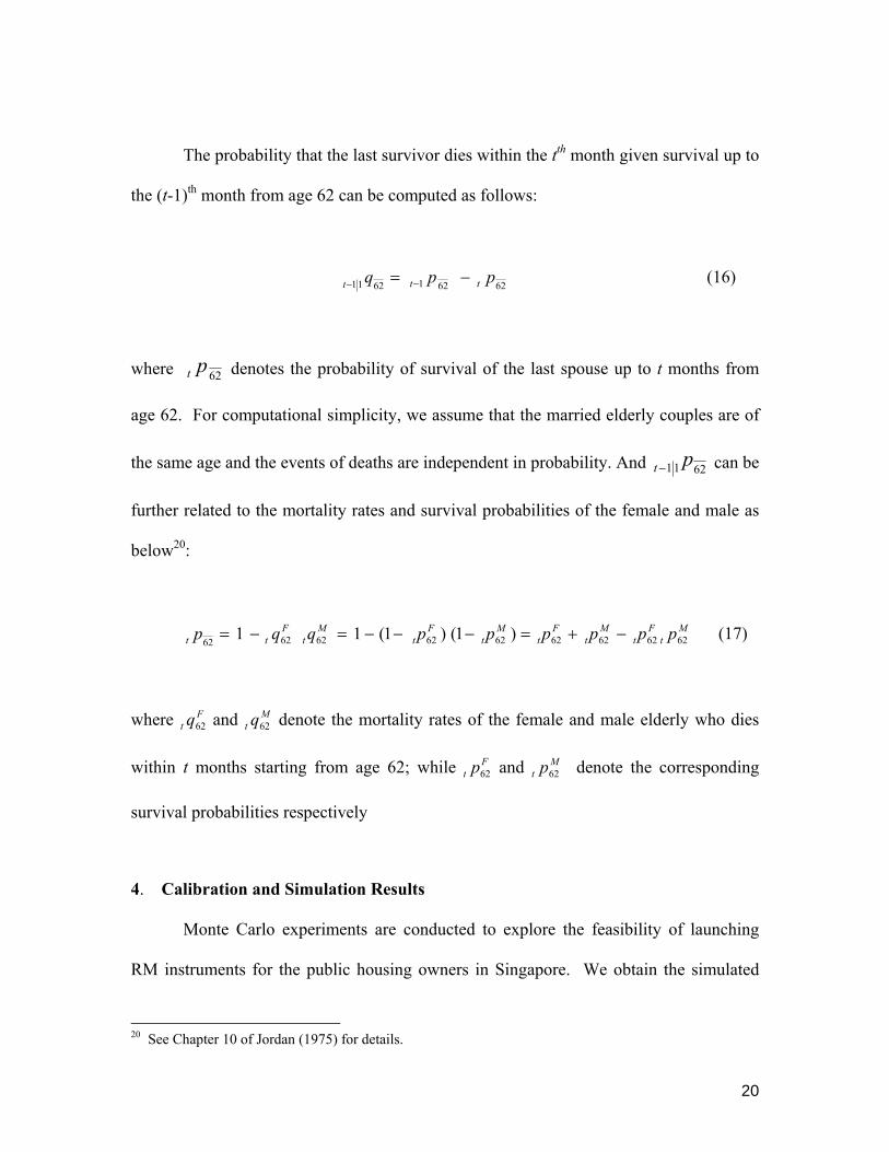
The probability that the last survivor dies within the tth month given survival up to
the (t-1)th month from age 62 can be computed as follows:
626216211 ppq ttt −= −− (16)
where 62pt denotes the probability of survival of the last spouse up to t months from
age 62. For computational simplicity, we assume that the married elderly couples are of
the same age and the events of deaths are independent in probability. And 6211 pt − can be
further related to the mortality rates and survival probabilities of the female and male as
t q62 denote the mortality rates of the female and male elderly who dies
within t months starting from age 62; while Ft p62 and M
t p62 denote the corresponding
survival probabilities respectively
4. Calibration and Simulation Results
Monte Carlo experiments are conducted to explore the feasibility of launching
RM instruments for the public housing owners in Singapore. We obtain the simulated
20 See Chapter 10 of Jordan (1975) for details.
21
values of Lt and Pt using equations (1) and (4) by alternative model parameterisations,
including different initial home values (P0), rates of property appreciation (α), interest
rate paths to reflect different risk premium, and joint cohort survival probabilities. All
computations and estimations are coded in Gauss. It is possible to generate infinitely
many interest-rate paths by the CIR model as described in equation (13), but we have
confined our simulation to 5,000 runs.
We choose the 4-room public housing owners as the benchmark household. This
is supported by the empirical evidence that the largest proportion of HDB owners (about
39%) in year 2002 are in 4-room flats. In fact, 68% of the residents are living in HDB 4-
room or larger flats or private housing, up from 52% in 1990. While a decade ago, the
greatest proportions of the HDB owners (about 35%) were in 3-room flats. Because of
greater affluence, 42% of these 3-room HDB owners have moved to 4-room or larger
flats or private properties in 2000.21 Table 2 shows the price range of the new 4-room
flats offered by HDB for different residential zone and town in 2000. In pricing new flats
for sale, HDB takes into consideration the affordability factor. The prices of new 4-room
flat are pegged to the average household income levels to ensure that at least 70% of all
household can afford to purchase a new 4-room flat. It also shows the average valuation
of resale flat at market prices, which varies according to location.22
21 See Singapore, Department of Statistics (2001), Table 10. 22 Since March 1971, a resale market in HDB flats emerged when owners of HDB flats were allowed to sell their flats at market prices. The government intervenes in the HDB resale market by setting the minimum occupancy period requirement before resale is possible. In 1971, the period was set at three years and was extended to five years in 1973. It has remained so until 1979 when it was relaxed to two and half year. The active resale HDB market has led to the sentiment that public housing has become “a cash cow for the milking of housing subsidies”. (The Straits Times, April 19, 1997). As of January 2003, the minimum occupancy period was further reduced to one year.
22
== Insert Table 2 ===
Table 3 describes the average floor area of the different public housing types and
the profile of the households in terms of the average annual household income for
different public housing types. The demand for RM is assessed by comparing monthly
annuity payments to the replacement incomes which are proportions of pre-retirement
household incomes. We set the benchmark mean household income at $3719 and the
median household income at $3000.23
== Insert Table 3 ===
Table 4 summarises the value of parameters used in the benchmark scenario. We
first estimate the accumulated loan amount (Lt) in equation (1) by setting various monthly
annuity payouts, starting from $900 and increasing it in steps of $100. For each level of
payout, we compute the associated net accumulated property value Pt which is given in
equation (4). As long as Pt exceeds Lt , the supplier will make a profit. However at a
first breakeven month m*, such that t > m*, Lt will exceed Pt. As can be observed from
Table 5, our simulation results are consistent with the intuition that the first breakeven
month for the supplier is sooner for the higher than the lower annuity payouts. Table 5
also tabulates the probability of loss for different levels of monthly annuity payouts,
using equation (6).
23 The Census of Population 2000 indicates that for the general population, the average household income in 2000 is $4,943 and the median household income is $3,607. But for HDB dwellers, the average household income is lower at $3,719 and the median household income is $3000. (HDB, 2000).
23
== Insert Table 4 ===
The present value of profit (PVP) in equation (10) depends on the stochastic
interest rate fluctuations. Using the CIR model as described in Section 3.3, we generate a
yield curve to obtain the corresponding PVP, and the whole process is run 5000 times to
obtain the mean value of PVP (MPVP). Table 5 also tabulates the values of MPVP, the
standard deviation of PVP and its values at the 5th and 95th percentiles as well as the
probability of loss and the first breakeven months at various monthly level annuities.
== Insert Table 5 ==
Table 5 shows that for an initial property value of $240,000 and a monthly
annuity level of $1500, the probability of loss for the supplier is only 0.0367, with a later
first breakeven month, occurring at m* = 478. However, when the monthly annuity
payout is increased to $1600, the probability of loss will be much higher at 0.5374, with
the first breakeven month occurring sooner at m* = 350. If the private RM supplier is
risk averse and prefers a smaller probability of loss, then he will set a lower level of
monthly annuity, say at $1000. But in this instance, there may be no demand for the RM
as the replacement ratio will be much lower than the expected 70%.24 Hence, the
completeness of the RM market depends on setting an annuity payout that is adequate to
finance retirement expenditure, while containing the probability of loss to the supplier.
24 There is no single acceptable replacement ratio. McGill et al., (1996) recommend using a replacement rate of 73%. In Canada, financial planners typically set a ratio of 70% of post-retirement income to maintain a comparable standard of living experienced before retirement.
24
Table 5 also indicates that when the monthly payout is increased to $1700 to
attain a replacement ratio of 46% of the pre-retirement average income, the probability of
loss to the supplier is higher at 0.8024. This is in stark contrast to the negligible
probability of loss when the monthly annuity payout is $1400. Hence, we may interpret
the difference of $300 as the loading factor levied by the RM supplier. The loading
factor can be as high as 21% ($300/$1400). Our findings are consistent with Caplin
(2002) and others who accord the incompleteness of the reverse mortgage market to high
loading factors.
We next evaluate the RM market when the supplier is a non-profit motivated
supplier, for example the government. As profit is not a major consideration for the
public provider, in our computation of the accumulated loan value (Lt) in equation (1),
risk-free interest rate r is used instead of the risk-embedded rate y which incorporates
both the risk premium and profit margin. For easy comparison, we define the breakeven
annuity as the annuity which yields zero MPVP for the private supplier. We repeat the
simulation process to obtain the new breakeven month for the public provider while
setting the payout at the breakeven annuity.
Table 6 tabulates simulation results which compare the adequacy of the RM
instruments provided by profit or non-profit motivated suppliers of RM. These include
the mean monthly payout at the breakeven annuity, its standard deviation, the 5th and 95th
percentiles, the probability of loss, the first breakeven month, and replacement ratio
based on the mean and median monthly income of the household. We repeat the
25
simulations using different initial property values assumption, ranging from $220,000 to
$300,000.
== Insert Table 6 ==
As can be observed from Table 6, for a given property value of $220,000, the
mean breakeven monthly payout is $1475. This level of the breakeven annuity represents
a replacement ratio of 49% of the average household income. However, there may be no
private supplier as the probability of loss is close to 0.581, implying that it is highly
probable that the accumulated loan balance is higher than the net value of the property at
the time of repayment. As such, it is interesting to know the possible effect of
government intervention in the market. Table 6 indicates that at the same average
breakeven annuity, the probability of loss for the public provider is now almost negligible
as the public provider has lower cost of fund and is able to charge the loan balance at the
risk free interest rate.
In addition, at a higher initial property value of $300,000, the homeowner can
expect to unlock the housing equity to yield an income which is almost 67% of the pre-
retirement average income. But again the market may be missing as the probability of
loss for the private supplier is still high at 0.586. However, the probability of loss is only
0.003 for a public provider. Furthermore, compared to the private supplier, the first
breakeven month for the public provider occurs 176 months later.
26
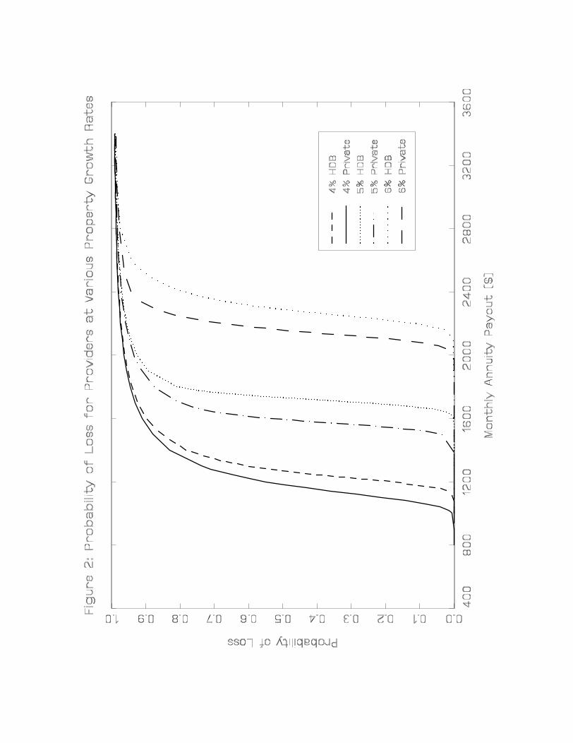
We concur that profitability is vital for the private RM suppliers but not so for the
public suppliers. Figure 2 displays the probability of loss for both the public and private
supplier using different levels of monthly annuity payouts. It also compares the
probability of loss for various property appreciation rates. As can be gleaned from Figure
2, the probability of loss is smaller at higher appreciation rates. For example, when the
annuity level is at $1600, the probability of loss for the private provider is 0.586 when α
is 5%. But at a higher appreciation rate at 6%, the probability of loss is lower at 0.476.
In addition, the probability of loss for a private supplier always lies to the left of that for a
public provider, implying that the public provider is able to support a reasonably higher
level of life annuity compared to the private supplier. Hence the market is more efficient
under a public than a private supplier.
== Insert Table 7 and Figure 2 ==
Both Figure 2 and Table 7 show that the completeness of the RM market depends
on the appreciation rates of the property. Table 7 shows that at α = 6%, the mean
monthly breakeven payout is $2154, hence implying a high replacement ratio of 72%.
This no doubt will attract a demand for RM. However, there may be no private supply as
the probability of loss is 0.476. This is due to the non-discourse nature of RM. However
at a lower appreciation rate of 3%, the mean monthly breakeven payout is $879,
representing a low replacement ratio of 30%. The probability of loss is 0.5 for the private
supplier and 0.296 for a public provider. This is clearly undesirable as even the public
provider will suffer a loss.
27
== Insert Figure 3 ==
Figure 3 plots the simulated first breakeven month m* at different monthly
annuity levels for both the public provider and the private supplier. As can be gleaned,
the higher is the appreciation rate, the higher the breakeven month. For example, using
the benchmark parameters, when α =5%, the average first breakeven month for the public
provider is at the 338th month compared to 511th month for the private supplier. With α =
6%, the first breakeven month for the public provider and the private supplier is at the
490th and 364th month, respectively.
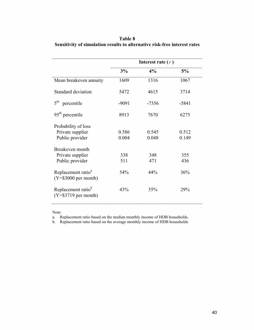
Table 8 presents simulation results using different risk-free interest rates at 3%,
4% and 5%, respectively. As the RM supplier charges a higher interest rate, the lower is
the mean breakeven payout annuity and RM becomes less adequate to finance retirement.
At the benchmark risk-free interest rate of 3%, the monthly annuity payout is $1609
which implies a replacement ratio of 54%. However at a higher interest rate of 5%, the
monthly payout is $1067, thereby implying a mere replacement ratio of 36%.
== Insert Table 8 ==
Moreover, values of the breakeven annuity are affected by various yield curves
used in the simulation exercises. Table 9 tabulates the simulated mean breakeven
monthly annuity payout with the yield curves generated by the Cox, Ingersoll and Ross
(CIR) stochastic model, fixed yield rate (FYC) and the constant yield curve (CYC)
28
models, respectively. In general both the CIR and FYC models give consistent values of
probability of loss and the first breakeven month. But values generated from the CYC
model deviate substantially from those generated from the CIR and FYC models. This
may due to using flat rates to discount cash flows.
== Insert Table 9 ==
5. Conclusion
We have examined the monthly annuity payouts in terms of replacement ratios
and drawn implications on the adequacy of RM in financing retirement needs. Using
Monte Carlo simulations, we compute the mean present value of profit for different levels
of annuity, the probability of loss and the first breakeven month. We compare the
viability of the RM under a private supplier with a public provider based on different
costs of capital. Such a comparison yields important policy implications on the need for
a low cost supplier.
Our simulation findings indicate that although most public housing homeowners
have their wealth tied up in their flats, property values are inadequate to support
retirement expenditure at the 70% replacement ratio. If these home owners are willing to
lower their expectation to attain at about 54% of the retirement income, then it is possible
to convert their house into a stream of future income by borrowing from the public
supplier. However, a replacement ratio at 54% may be moderately low compared to the
recommended ratio of 70% in most of the developed countries. But there are alternative
29
sources of retirement income in Singapore. For example, an important source is family
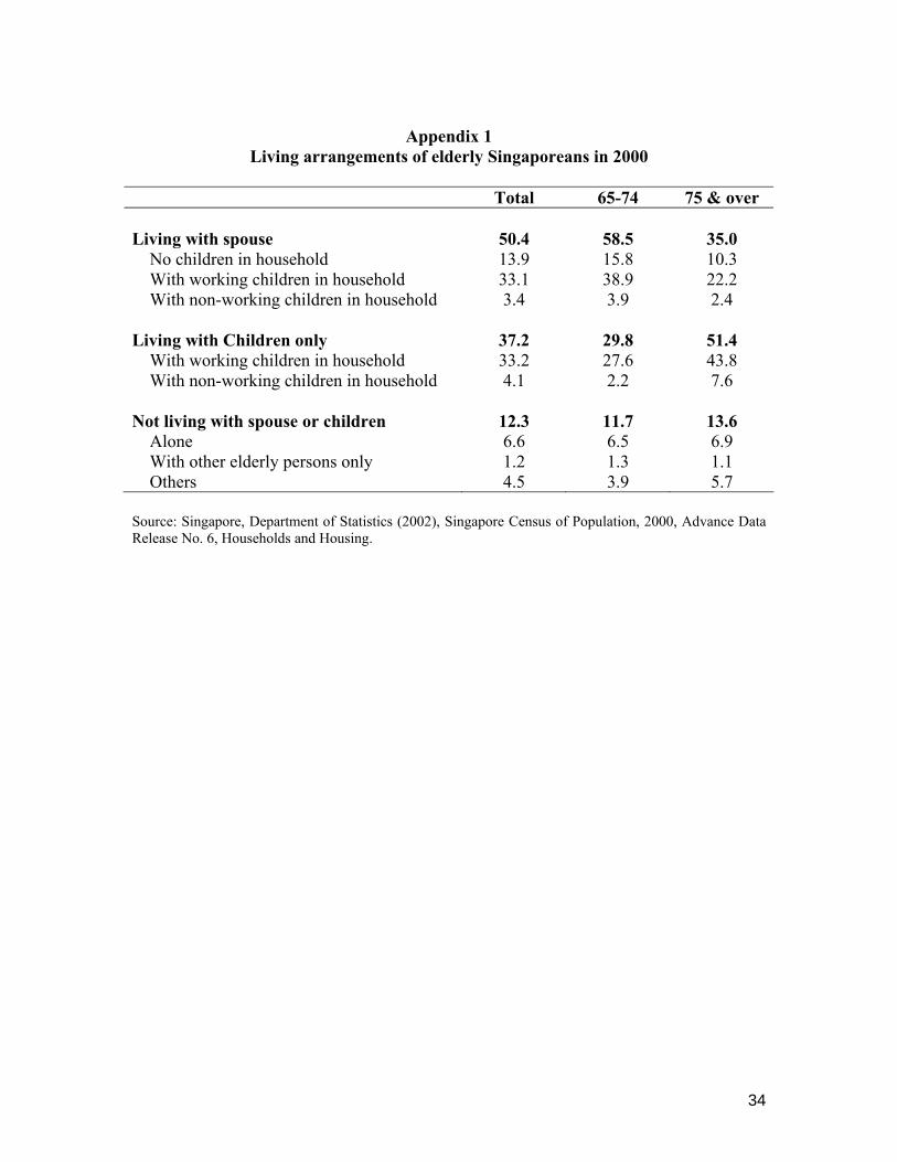
support, particularly from children.25 The living arrangement among the elderly testifies
to strong family support. As can be observed from Appendix 1, less than 13% of the
elderly are not living with spouse or children. Only 6.6% of the elderly live alone. In
2000, about 60% of the elderly live with their working children. This is especially so for
the elderly aged 75 and over, as about 50% of them live with their children.
Our study is not without caveats. For instance, we have not factored in the tenure
of HDB flats. As most HDB flats are on lease for 99 years, finance companies may not
be willing to take on a flat with less than 60 years left on the tenure. Another possible
financing option is for homeowners to down-grade to smaller flats and to convert the
financial gains from the sales of flats into some forms of annuity instruments. In fact, in
March 1998, HDB introduced the Studio Apartment Scheme, whereby the elderly flat
owners could sell off their flats in the resale market and use part of the proceeds to buy a
smaller studio apartment from HDB.26 The remaining fund may be used to top up their
medical savings account to ensure that the elderly have adequate funds to meet their
medical needs or it may be invested in annuities which yield regular monthly income.
Furthermore, since October 2003, many HDB-imposed restrictions on public housing
were lifted, thereby allowing flat owners to monetise their assets by subletting the entire
flats.
25 Singapore has a Parents Maintenance Bill, which stipulates that children are legally obliged to care for their elderly parents. 26 The studio apartments are smaller, which come in two sizes: 35 to 45 sq m. They are specially equipped with elderly-friendly features and are sold on a 30-year lease.
30
Another caveat is that we have excluded other social dimensions which could
possibly affect the success of reverse mortgages. These factors include bequest motives
and the psychological reluctance among the elderly to mortgage their homes to financial
institutions. Such social norms are likely to prevail so that even with a public provider,
the reverse mortgage market may still remain thin. However, these issues are left for
future investigation.
31
References
Asher M.G. and Phang S.Y. (1997). Singapore’s Central Provident Fund system: implications for saving, public housing and social protection. In Andersson, A.K., B. Harsman and J.M. Quigley. Government for the Future: Unification, Fragmentation and Regionalism. Amsterdam: North Holland. Beal D. J. (2001). Home equity conversion in Australia – Issues, impediments and possible solutions. Manuscript, University of Southern Queensland. Boehm, T and M. Ehrhardt (1994). Reverse mortgages and interest rate risks. Journal of the American Real Estate and Urban Economics Association, 22(2), pp 387 – 408. Bourbeau, R, J. Legare and V. Emond (1997). New birth cohort life tables for Canada and Quebec, Demographic Document, No.3, Demography Division, Statistics Canada. Campbell, J.Y., A.W. Lo and C. MacKinlay (1997) The Econometrics of Financial Markets. Princeton: Princeton University Press. Caplin A (2002). Turning assets into cash: Problems and prospects in the reverse mortgage market in O.S. Mitchell et al. Innovations in Retirement Financing, Philadelphia, PA: University of Pennsylvania Press, 2002. Chia N.C. and A.K.C. Tsui (2003a). Life annuities of compulsory savings and income adequacy of the elderly in Singapore. Journal of Pension Economics and Finance, March 2003. Chia N.C. and A.K.C. Tsui (2003b). Medical savings accounts in Singapore: How much is adequate? Manuscript. June 2003. Cox, J.C., J.E. Ingersoll and S.A. Ross (1985). A theory of the term structure of interest rates. Econometrica 53, 385-407. Gibbs I. (1992). A substantial but limited asset: the role of housing wealth in paying for residential care in J Morten (ed.) Financing Elderly People in Independent Sector Homes: The Future, London: Age Concern Institute of Gerontology. Hancock R. (1998). Can housing wealth alleviate poverty among Britain’s older population? Fiscal Studies 19(1), 249-272. Jordan, C. W. (1975). Life Contingencies. The Society of Actuaries, USA. Kutty N.K. (1998). The scope for poverty alleviation among elderly home-owners in the US through reverse mortgages. Urban Studies 35(1), 113-130.
32
Lachance M.E. and O. Mitchell (2002). Guaranteeing defined contribution pensions: The options to buy-back a defined benefit promise. NBER Working Paper 8731. Lee, R. D. and L. Carter (1992). Modeling and forecasting the time series of U.S. mortality. Journal of the American Statistical Association 87, 659-71. Mayer, C. and K. Simons (1994). Reverse mortgages and the liquidity of housing wealth. Journal of American Real Estate and Urban Economics Association 22 (2), 235-255. Merrill S. R., M. Finkel and N. Kutty (1994). Potential beneficiaries from reverse mortgage products for elderly homeowner: An analysis of American Housing Survey Data. Journal of American Real Estate and Urban Economics Association 22(2), 257-299. McCarthy, D., O. Mitchell and J. Piggott. (2002). Asset rich and cash poor: retirement provision and housing policy in Singapore. Journal of Pension Economics and Finance. 1(3), 197-222. McGill, D., K. Brown, J. Harlely and S. Scheiber (1996). Fundamentals of private pensions. 7e. University of Pennsylvania, Philadelphia, PA. Mitchell O. and J. Piggott (2003). Unlocking housing equity in Japan. Centre for Pensions and Superannuation Discussion Paper 03/01. Noguchi Y. (1997). Improvement of after-retirement income by home equity conversion mortgages: possibility and problems in Japan in Michael D. Hurd and N. Yashiro (eds) The Economic Effects of Aging in the United States and Japan. Chicago University Press. Porteba, J.M. (2001). Taxation, risk-Taking and household portfolio behaviour. National Bureau of Economic Research Working Paper 8340. Phang S.Y. and A. Tan (1991). The Singapore Experience in Public Housing. Times Academic Press, Singapore, 1991, 49 pages. Phang S.Y. (1996). Economic development and the distribution of land rents in Singapore: A Georgist implementation. The American Journal of Economics and Sociology. Vol 55 pp.489-501. Philips, W. and S. Gwin (1993). Reverse mortgages, Transactions Society of Actuaries, Vol. XLVIV, pp. 289-323. Pollard, J.H. (1989). On the derivation of a full life table from mortality data recorded in five-year age groups. Mathematical Population Studies 2(1), 1-14. Sheiner, L. and D. Weil (1993). The housing wealth of the aged. National Bureau of Economic Research Working Paper 4115.
33
Singapore, Department of Statistics (2001). Census of population 2000: Households and housing : Statistical Release 5. Singapore National Printers. Singapore, Department of Statistics (2003). Statistical Highlights 2000/01 Singapore National Printers. Singapore, Department of Statistics (2003). Wealth and liabilities of Singapore household Occasional Paper on Economic Statistics. Singapore National Printers. Singapore, Housing Development Board (2000). Profile of residents living in HDB flats. Singapore National Printers. Singapore, Housing Development Board (2001). Annual report 200/01 Singapore National Printers. Singapore, The Straits Times. Various dates. Singapore: Singapore Press Holdings. Tse, Y.K. (1995a). Stochastic behaviour of interest rates in Singapore. Advances in Pacific Basin Financial Markets 1, 255-276. Tse, Y.K. (1995b). Modelling reverse mortgages. Asia Pacific Journal of Management 12(2), 79-95. Tuljapurkar, S., N. Li and C. Boe (2000). A universal pattern of mortality decline in G7 countries. Nature 45, 509-538. Venti S. and D. Wise (1991). Ageing and the income value of housing wealth. Journal of Public Economics 44(3), 371-397. Venti S. and D. Wise (2001). Ageing and housing equity: Another look. National Bureau of Economic Research Working Paper 8608. Wilmoth, J. R. (1995). Are mortality rates falling at extremely high ages? An investigation based on a model proposed by Coale and Kisker. Population Studies 49, 281-295.
34
Appendix 1
Living arrangements of elderly Singaporeans in 2000
Total 65-74 75 & over Living with spouse
50.4
58.5
35.0
No children in household 13.9 15.8 10.3 With working children in household 33.1 38.9 22.2 With non-working children in household 3.4 3.9 2.4 Living with Children only 37.2 29.8 51.4 With working children in household 33.2 27.6 43.8 With non-working children in household 4.1 2.2 7.6 Not living with spouse or children 12.3 11.7 13.6 Alone 6.6 6.5 6.9 With other elderly persons only 1.2 1.3 1.1 Others 4.5 3.9 5.7
Source: Singapore, Department of Statistics (2002), Singapore Census of Population, 2000, Advance Data Release No. 6, Households and Housing.
35
Table 1
Household residential property asset ratios in 2000
Housing Assets/ Total Assets
(%)
Housing Assets/ Personal Disposable
Income (%)
Housing Assets/ GDP (%)
Singapore 51 452 230 United States 28 155 113 Japan 40 294 198 France 47 271 176 United Kingdom 39 292 197
Source: Singapore, Department of Statistics (2003). Wealth and Liabilities of Singapore Household, Occasional Paper on Economic Statistics.
Table 2 Sample of price range of flats offered by HDB and
Average valuation of resale flat in 2000
Town HDB list price ($) Resale price($) Sembawang 98,000 – 162,000 204,000 Jurong West 99,000 – 56,000 186,100 Woodlands 104,000 – 151,000 192,500 Choa Chu Kang 110,000 – 162,000 217,200 Bukit Panjang 110,000 – 166,000 187,400 Seng Kang 120,000 – 186,000 228,100
Source: Singapore, Housing Development Board, Annual Report. 2000/01 and HDB Average Valuation by town and flat types, available at: http://www.hdb.gov.sg
36
Table 3
Profile of household by housing types in Singapore
Note: Household incomes are estimated based on the 1997/98 Department of Statistics (DOS) Household Expenditure Survey (HES) and adjusted to 2001 levels.
Table 4 Values of parameters for the benchmark scenario
(i) Age of mortgagor at the first monthly annuity payout = 62 (ii) Typical mortgagor is a 4-room HDB dweller Average pre-retirement household income = $3,719 Median pre-retirement household income = $3,000 (iii) Initial appraised property value of the 4-room flat (P0) = $240,000 Annual growth rate of the property (α) = 5% Initiation fee (λ) = 1% of the appraised value of the property Closing fee (τ) = 3.5% of the selling price of the property (iv) Risk-free interest rate or cost of capital (r) = 3 % Cost of capital to RM private supplier (y) = r + 1% Cost of capital to RM buyer (i) = r + 2% (v) Cox-Ingersoll-Ross model of stochastic interest rates: Initial interest rate = 3% Average interest rate (ra) = 3% __________________________________________________________________
37
Table 5
Present value of profit, probability of loss for private RM suppliers using benchmark parameters
Probability of loss and first breakeven month under private and public RM suppliers using different initial property values
Initial property value
$ 220K $ 240K $ 260K $ 280K $ 300K
Mean payout of breakeven annuity
1475 1609 1743 1876 2011
Standard deviation
5010 5472 5894 6260 6675
5th percentile
-8106 -9091 -9752 -10233 -11274
95th percentile
8368 8913 9448 9791 10887
Probability of loss Private supplier 0.581 0.586 0.585 0.584 0.586 Public provider Breakeven month Private supplier Public provider Replacement ratioa (3000 per month)
0.004
339 511
49%
0.004
338 511
54%
0.004
338 511
58%
0.004
338 511
63%
0.003
338 514
67%
Replacement ratiob ($3719 per month)
40% 43% 47% 50% 54%
Note: a. Replacement ratio based on the median monthly income of HDB households. b. Replacement ratio based on the average monthly income of HDB households.
39
Table 7
Probability of loss and first breakeven month under private and public RM suppliers using different property appreciation values
Rates of property appreciation (α)
3% 4% 5% 6%
Mean payout of breakeven annuity
879
1194
1609
2154
Standard deviation
2714 3814 5472 7321
5th percentile
-4595 -6066 -9091 -12202
95th percentile
4534 6087 8913 11919
Probability of loss Private supplier 0.500 0.535 0.586 0.476 Public provider Breakeven month Private supplier Public provider
0.296
358 401
0.154
350 435
0.004
338 511
0.019
364 490
Replacement ratioa
($3000 per month)
30% 40% 54% 72%
Replacement ratiob ($3719 per month)
24%
32% 43% 58%
Note: a. Replacement ratio based on the median monthly income of HDB households. b. Replacement ratio based on the average monthly income of HDB households.
40
Table 8
Sensitivity of simulation results to alternative risk-free interest rates
Interest rate ( r )
3% 4% 5%
Mean breakeven annuity
1609 1316 1067
Standard deviation
5472 4615 3714
5th percentile
-9091 -7356 -5841
95th percentile
8913 7670 6275
Probability of loss Private supplier Public provider
0.586 0.004
0.545 0.048
0.512 0.149
Breakeven month Private supplier Public provider
338 511
348 471
355 436
Replacement ratioa (Y=$3000 per month)
54% 44% 36%
Replacement ratiob (Y=$3719 per month)
43%
35% 29%
Note: a. Replacement ratio based on the median monthly income of HDB households. b. Replacement ratio based on the average monthly income of HDB households
41
Table 9
Sensitivity of simulation results to different interest rate models
Note: The mean first breakeven month at the corresponding breakeven annuity are computed using three different yield curve models. CIR represents the yield curve generated by the Cox, Ingersoll and Ross model; CYC is the flat 4% yield curve and FYC is the fixed yield curve based on the mean spot rates of government bonds with various durations. A is the mean level monthly payout, α is the property appreciation rates.
42
Figure 1: Percentage of population housed in HDB flats
86% 85% 87%
81%
67%
9% 23%
35% 47%
0
20
40
60
80
100
1960 1965 1970 1975 1980 1985 1990 1995 2001(Mar)
Year
Estimated percentage of resident population living in HDB flats
Source: Singapore, HDB Research & Planning Department.
Note: Data from 1960 to 1979 refer to Total Population (including both residents and non-residents. From 1980 onwards, the data refer to Resident Population only (i.e. Singaporeans and permanent residents) and exclude non-residents.