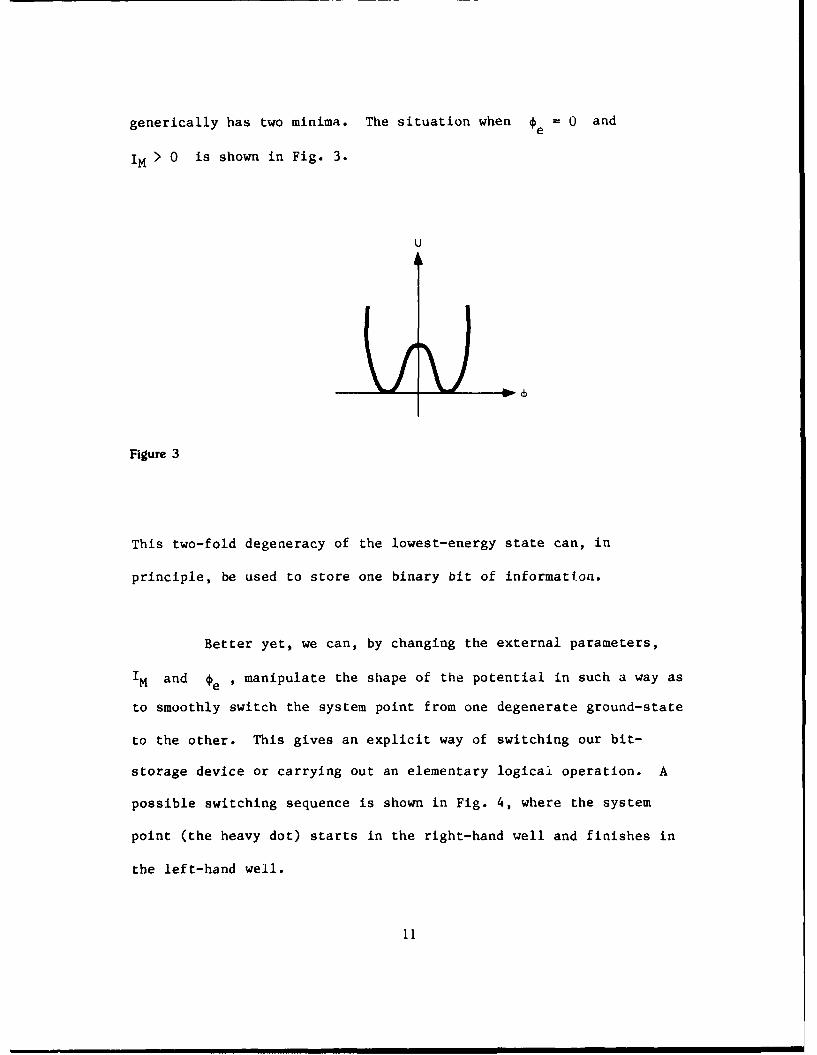
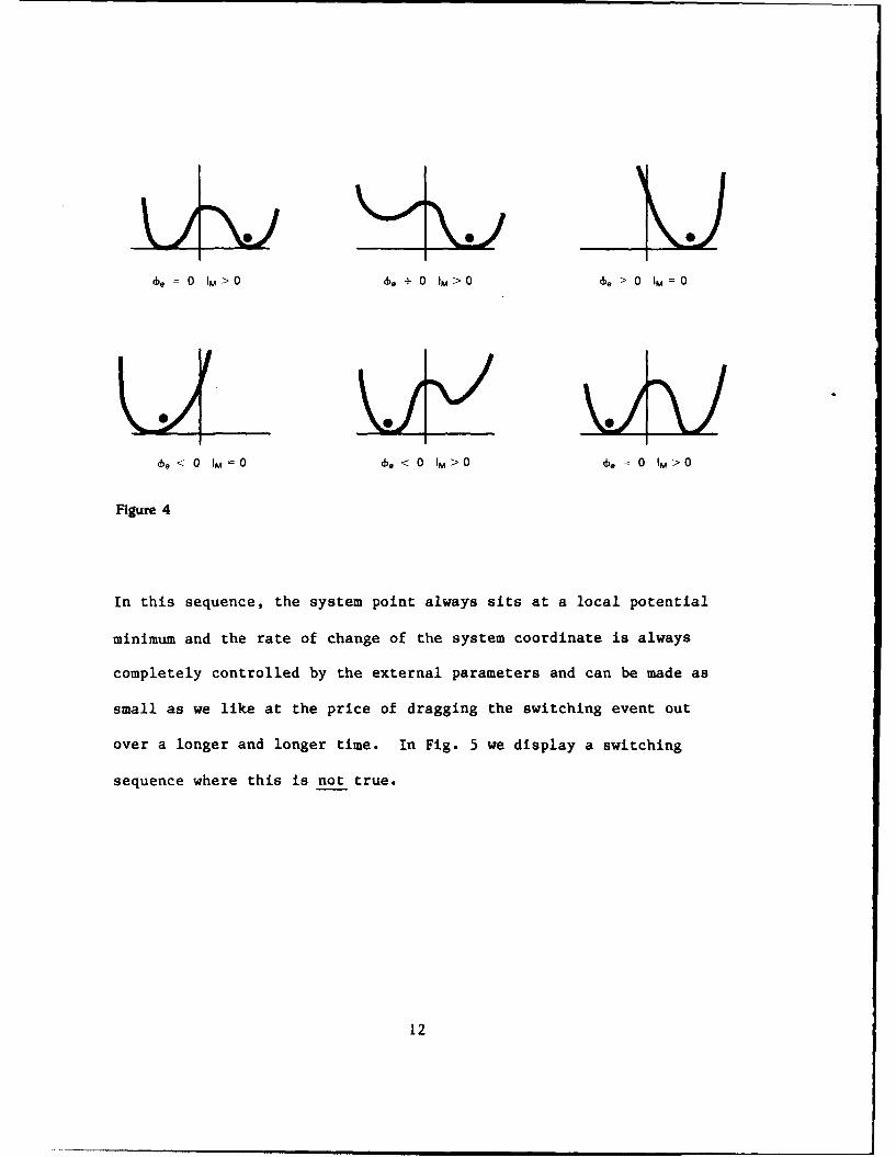
Reversible Logic as a Strategyfor Computing
C% C. CallanAccesion For
-NTIS ,CRA&I
CNDTIC TABD-~ U.oa-mouliced
Justifica,i.......
ByDist, ibutiof
AvailabilityC.
Dist Avail a d IorSpL:ciai
January 1984 LA tJSR-83- 112
JASONThe ME Corporation
1820 Dolley Madison BoulevardMcLean. Virginia 22102
REVERSIBLE LOGIC AS A STRATEGY FOR COMPUTING
During the 1983 Summer Study, a few members of JASON
attempted to survey the current status of the reversible logic
approach to digital computing. Our aim was to form an opinion on
which future developments of this subject might be relevant to
DARPA's computer-related interests and possibly worthy of its
support. We consulted one of the pioneers in this subject, Dr.
Edward Fredkin of MIT, at some length and brought ourselves up to
date on the (not very extensive) literature. Our basic conclusion
is that the importance of reversible logic depends crucially on the
physical architecture of the computer: It is irrelevant to the
current scheme in which packets of charge are stored on, and moved
between, structures of order one light wavelength in size, but might
be relevant and even essential if the basic information-handling
units were of molecular or atomic size (a distant but not
necessarily-unattainable goal). The question of physical
realization of reversible logic elements has been almost completely
neglected* in favor of the abstract questions of how, given the
existence of reversible logic elements, one could wire them up to
make a useful computer and how one would program it. We think that
*Apart from some interesting "existence proof" work ot Fredkin et
al.7
1 /
>
I
the problem of how to physically realize reversible computation at
something like the atomic scale should be the next question to be
attacked in this area. We also think that the very framework of
reversible logic suggests some interesting new approaches to the
problem of ultra-small-size computing elements which might be worth
exploring for their own sake. Although practical payoff on any of
these ideas is surely far off, the computer science and physics
issues raised are fascinating and of fundamental importance.
Investigations in this area are probably deserving of DARPA support
as topics in pure computer science. The body of this report
amplifies these remarks.
Energy Dissipation in Computing
Contemporary computers dissipate at least 10- 12 joules
(about 108 kT, if T equals room temperature) per logical
operation. The reason is that bits are stored as charges on
capacitors charged to about one volt (the typical operating voltage
of solid state electronic devices). Since there is a lower limit to
the size and capacitance of circuit elements that can be fabricated
on a chip using optical techniques, there is a lower limit to the
energy associated with storing one bit. That limit turns out to be
the above-mentioned 1012 joules, and the current style of computer
logic causes that entire energy to be dissipated each time the state
2
of a bit is changed. 1 The resulting heat load is a major barrier to
high speed computation.
A major question is the extent to which this dissipation is
an inescapable concomitant of computation and to what extent it is
due to "inefficient" physical or logical design of the computer.2
Information theoretic/thermodynamic arguments have been used to
suggest that there is a fundamental dissipation limit of kT per
operation for computers designed on current principles.
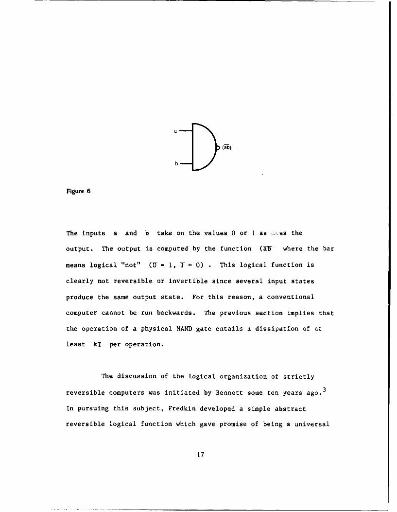
In thermodynamics there is a well-known connection between
dissipation and reversible operation of heat engines. Standard
computer logic elements, the NAND gate in particular, are not even
reversible as abstract logical operations, let alone as physical
devices. It has been suggested that if reversible logic functions
are used, it is, in principle, possible to do computing with zero
dissipationl3 ,4 In this scenario, the entire computing operation
would have to be carried out reversibly in analogy with the
dissipationless operation of a reversible heat engine.
It is hard to evaluate the relative merits of two schemes
which promise to reduce dissipation to U • kT (the claimed limit
for reversible logic) and I - kT (the claimed limit for standard
logic) per operation, respectively, when the best dissipation
3
achieved to date is 108 kTI We think it is worthwhile to pursue the
reversible logic scenario, not so much because it promises superior
practical benefits, but rather because it raises unfamiliar
questions about the nature of computing and suggests some
interesting new approaches to the physical realization of
computation.
There are two types of questions which arise when you
pursue this line. First, there are the questions of what are useful
reversible logic functions, how might they be tied together to make
a useful computer, and how might such a computer be programmed.
These questions are all answerable in the abstract, without any
reference to the physical realization of the system. This sort of
question is the major subject of the work of Fredkin and other
pioneers in reversible logic and the results are that manageable
reversible logic computers can be designed, although they are in
many interesting ways different from conventional computers. The
second question has to do with physical realization of reversible
computation. What sort of physical system can be used, what
calculation speeds can be achieved, etc.? Here very little is
known, although many interesting questions arise. We think this is
the most important aspect of the reversible computation problem and
have attempted to construct a framework for a serious exploration of
these questions.
4
Physical Realizations of Computers
To establish a useful framework for our discussion, it is
helpful to remark that there are at least two broad classes of
physical realizations of computing machines. The most important
distinction is between open (dissipative) systems and closed
(conservative) systems. The distinction is between systems in which
the computational degrees of freedom are coupled to a "heat bath"
with which energy can be exchanged and systems in which the
computational degrees of freedom are effectively isolated from the
rest of the world. The other essential distinction is between
systems in which the computational degrees of freedom can be
described classically versus those in which they must be described
quantum mechanically.
A dissipative system will behave in many respects like a
heat engine. In particular, it should be possible to design it so
that it is more and more reversible and less and less dissipative
the slower it runs. This suggests an interesting tradeoff between
dissipation and speed of operation, about which we will be more
quantitative in the next section. (The logical architecture of such
a machine could be either reversible or not.)
A conservative system is necessarily reversible because any
closed Hamiltonian system is reversible. In fact, it is physically
5
reversible whatever its speed of operation, and it would hardly make
sense for the logical architecture of such a machine to be anything
other than reversible!
Any device in which the computational degrees of freedom
are realized on a scale much larger than atomic size will inevitably
be dissipative: the total number of physical degrees of freedom
vastly outnumber those directly involved in computation, and it is
impossible to prevent leakage of energy between the computer and the
"heat bath." This is the case with all present-day machines.
On the other hand, if the computational system were
realized at the atomic scale, as some kind of cleverly constructed
lattice, for instance, then the computational degrees of freedom
would be a major fraction of the total number of degrees of
freedom. In that case, the system might function as a good
approximation to a closed reversible Hamiltonian system, and the
choice of reversible logic structure would be essential. Needless
to say, no one has any practical ideas on how to realize such a
computing system, though, of course, the entire thrust of the
development of faster computation is toward physically smaller
computing elements. The point is that if atomic scale computing
elements are ever constructed, reversible logic ideas may be most
appropriate to doing computation with them.
6
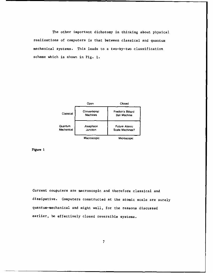
The other important dichotomy in thinking about physical
realizations of computers is that between classical and quantum
mechanical systems. This leads to a two-by-two classification
scheme which is shown in Fig. I.
Open Closed
Conventional Fredkin's BilliardClassical Machines Ball Machine
Quantum Josephson Future AtomicMechanical Junction Scale Machines?
Macroscopic Microscopic
Figure 1
Current computers are macroscopic and therefore classical and
dissipative. Computers constructed at the atomic scale are surely
quantum-mechanical and might well, for the reasons discussed
earlier, be effectively closed reversible systems.
7
Non-dissipative classical systems are consistent with
Newtonian mechanics and represent internally consistent idealized
systems which turn out to be a useful framework for demonstrating
general features of reversible computation. We will be discussing
Fredkin's billiard ball model in that light. Finally, there exist
macroscopic (i.e., dissipative) but quantum-mechanical logic devices
based on the Josephson junction which we will use to illustrate more
precisely the theoretical limits on dissipative devices.
Theoretical Limits for Dissipative Devices
The single junction superconducting interferometer provides
an example of a dissipative logic device whose properties can be
quantitatively analyzed in some detail. In this section, we
summarize the results of Likharev5 on the device schematized in
Fig. 2.
8
ICI
Figure 2
It consists of a superconducting ring, broken by a Josephson
junction (the cross in the figure), with provision for controlling
the maximum current, IM , that can flow through the junction by
varying an external current, Ic . The superconducting ring is
subject to an external magnetic field with a flux, fe I through the
ring. The ring carries a current, I , and has a net flux, , due
to the combined effects of I and *e through it. If the self-
inductance of the ring is L , the net flux satisfies
*= e -LI
9
The net flux, * , is proportional to 6 , the difference of the
superconducting order parameter phase across the junction and can be
thought of as the variable describing the "state" of this system.
To be precise, 6 = 2w /o , where * - 1 is the magnetic fluxo 2e
quantum. The system is made to function as a logic device by
manipulating the state variable through changes in the external
parameters Ic and e
The energy of this system is the sum of the magnetic field
energy
1 2 1 2UM =- LI - M ( 0 - e)
and the energy of a junction with a phase difference 6 across it
UJ3 + I 2 2w cos6
= IM o/2w cos(2w*/o )o
( IM is the maximum junction current which, as we have said, can be
manipulated from the outside.) The total energy functional,
1 (0 - Oe)2 +IMo 2wo
U( ) C o + -cos
10
I
generically has two minima. The situation when e 0 and
IM > 0 is shown in Fig. 3.
U
Figure 3
This two-fold degeneracy of the lowest-energy state can, in
principle, be used to store one binary bit of information.
Better yet, we can, by changing the external parameters,
IM and *e 9 manipulate the shape of the potential in such a way as
to smoothly switch the system point from one degenerate ground-state
to the other. This gives an explicit way of switching our bit-
storage device or carrying out an elementary logicai operation. A
possible switching sequence is shown in Fig. 4, where the system
point (the heavy dot) starts in the right-hand well and finishes in
the left-hand well.
11
de 0 IM >0 e+ 0 IM >0 (b > 0 IM = 0
KU~6e < 0 1M= 4b,
< 0 IM>O 4 0 IM>O
Figure 4
In this sequence, the system point always sits at a local potential
minimum and the rate of change of the system coordinate is always
completely controlled by the external parameters and can be made as
small as we like at the price of dragging the switching event out
over a longer and longer time. In Fig. 5 we display a switching
sequence where this is not true.
12
be = 0 'M>O (be<o IM> 0 be<0 'M>0
de < 0 IM - 0 (eb< >0 0 IM > 0
Figure 5
In the third step of this sequence, when the barrier finally
disappears, the system point is at a large positive energy with
respect to the left hand minimum. It will roll down the hili and
eventually settle down in the left-hand minimum only after
dissipating its extra energy. The rate of this motion and the
energy dissipated in it are not controllable from the outside, and
to minimize dissipation in switching we must avoid this sort of
sequence.
We finally come to the quantitative evaluation of
dissipation in the switching event. This device has many more
13
coordinates than the single flux coordinate, * , in which we are
primarily interested. The effect of these degrees of freedom can be
summarized by a viscous force
Fv =- K
which leads to damping of notions of the system coordinate (and
dissipation of energy from the * degree of freedom) at a rate
determined by K • The total energy loss in some time evolution of
is just
w-- fdtF +Kfdt ; >0
It is particularly convenient to characterise the damping
by the time, T , it takes small amplitude oscillations about ac
minimum to decay by e- l . In either of the switching scenarios
described above, $ necessarily is non-zero and there is
necessarily some dissipation. The shape of the potential during the
switching event is constrained by the requirement that spontaneous
switching into the wrong well due to classical thermal fluctuations
must be negligible (this means that the energy barrier between the
two local minima must always be much greater than kT ).
14
Given this information, it is a straightforward matter to
calculate the minimum energy dissipation (corresponding to the
sequence of Fig. 4) in a switching event carried out in a time
interval T . The result is, roughly,
T
W - kT .- cT
so long as T > T . In other words, the total energy dissipated in
a switching cycle can be made as small as we like by making the
switching time arbitrarily long compared to the basic dissipation
time scale. This is analogous to the situation with heat engines:
dissipation or entropy production can be made arbitrarily small by
running the engine arbitrarily slowly. We can also determine the
energy dissipated in a switching cycle like that of Fig. 5. In that
case it turns out that
W > kT
no matter how slowly we carry out the transition (at some stage the
system executes free fall down a potential hill whose height is
scaled by kT so that the system must dissipate energy of order
kT to come into equilibrium).
15
When this sort of device is used to make a computer, the
question of overall logical organization inevitably arises. It
turns out that if we use the conventional organization based on
(logically irreversible) NAND gates (which can be simulated by
appropriately connecting together several of the above-described
switches), then switching cycles of the type of Fig. 5 are
inescapable and dissipation at the rate of roughly kT per
operation is the theoretical limit. However, if a logically
reversible organization is used, it turns out that only switching
sequences of the type of Fig. 4 need be encountered and the
dissipation per operation can be reduced arbitrarily below kT , at
the price of reducing the rate of computation. Since the motivation
for reducing dissipation was to increase the rate of computation,
this seems rather self-defeating. Later on we will discuss
possibilities in which, at least in principle, dissipationless
reversible computation can be carried out at arbitrary speed. In
the next section we will finally make explicit what we mean by
reversible logical architecture and devices.
Reversible Computation-Abstract Issues
It is a commonplace of computer science that a computer can
be built entirely out of a Boolean logic device called a NAND
gate. The action of such a device is symbolized in Fig 6.
16
a
b:D (ab)
Figure 6
The inputs a and b take on the values 0 or I as .oies the
output. The output is computed by the function (af where the bar
means logical "not" (U = 1, T = 0) . This logical function is
clearly not reversible or invertible since several input states
produce the same output state. For this reason, a conventional
computer cannot be run backwards. The previous section implies that
the operation of a physical NAND gate entails a dissipation of at
least kT per operation.
The discussion of the logical organization of strictly
reversible computers was initiated by Bennett some ten years ago.3
In pursuing this subject, Fredkin developed a simple abstract
reversible logical function which gave promise of being a universal
17
building block for reversible computers.4 The structure and action
of this function, called the Fredkin gate, is shown in Fig. 7.
a a
b ab + ac
c 5b + ac
Figure 7
As in the case of the NAND gates, the input and output lines take on
the values 0 or 1. An examination of the truth table for this
device shows that it is invertible: the correspondence between
input and output states is one-to-one.
By ignoring some outputs and fixing some inputs, the
Fredkin gate can be made to perform any standard logical function.
For instance, the AND of a, b can be obtained by setting c = 0
and keeping only the middle output line, as in Fig. 8.
18
a
aa
abb ab
b
0 ab
Figure 8
This procedure requires a supply of input constants and a way of
disposing of the unwanLed outputs, known as "garbage." The brute
force method of carrying out reversible computation is to record
every one of the garbage constants which is produced during a
computation. This is not a very satisfactory proceeding since the
number of elementary logical operations required to carry out even a
simple arithmetic operation, let alone a complicated program, is
enormous and memory resources would be swamped.
Fredkin, Toffoli, and students have shown how to get round
this problem by really making use of the reversibility of the
system.6 ,7 The point is that if one is doing some machine
instruction such as computing the sum of two numbers which involves
a large number of logical operations, one may a) do the calculation,
19
producing a large quantity of garbage; b) record the result,
producing a very small amount of garbage; c) run the computation
backwards, eating up the garbage produced in a). If the machine
instruction itself is logically reversible, as in
(A,B) + ( A+B ), one doesn't even have to accumulate garbage in
step b). The only true garbage which needs special memory
allocation and has to be kept to the end of the program is that
associated with truly non-invertible machine instructions. By
careful design of the machine instruction set and programming
practices, it appears possible to reduce the garbage accumulated in
a typical program to a manageable size. We are not aware of a
quantitative answer to the question, if a program requires a total
of N steps to execute, what is the minimum number of garbage bits
that must be accumulated? We suspect that the answer is log N,
which would mean that only a trivial amount of memory has to be
devoted to true garbage accumulation, but we don't have a proof.
Finally, as a result of this experience, Fredkin and
students have been able to produce sketchy but credible designs for
real computers. These designs are explicit two-dimensional wiring
diagram layouts of Fredkin gates, and have been demonstrated in
computer simulation exercises to work as expected.
20
To summarize, although computers based on reversible logic
elements have some unfamiliar features, machines whose effective
operation is nearly a carbon copy of conventional computers can be
laid out as explicit two-dimensional hookups of the logically
reversible Fredkin gate. In the next section we will take up the
question whether the Fredkin gate is physically realizable.
Physical Realization of the Fredkin Gate
In order to give an existence proof for reversible
computation, Fredkin has introduced a stylized model based on
perfectly elastic collisions of billiard balls moving on a
frictionless plane. 4 Consider a two-dimensional square grid as laid
out in Fig. 9a, with unit spacing between the grid points and with
identical hard spheres of radius 1//2 moving at one lattice
spacing per time step along the principal directions of this lattice
(again, as shown in Fig. 9a). At time t = 0 , the center of every
ball lies on a grid point and that will again be true at every
integer-valued time. Balls will occasionally undergo right-angle
elastic collisions at integer-valued times (Fig. 9b).
21
0
* 0
9a 9b
Figure 9a,b
The balls emerging from the collision will again move along the
principal lattice directions and their centers will coincide with
lattice points at integer-valued times. At some lattice points a
billiard ball will be nailed down to function as a perfect reflector
of anything that comes by. The presence or absence of a billiard
ball at a lattice site at an integer time can be taken as a binary
bit of information and the Newtonian evolution of such a system of
billiard balls amounts to a "calculation" involving those bits.
The construction of the billiard ball realization of the
Fredkin gate goes in two steps. First, construct the gate shown in
Fig. 10 (called the interaction gate) where the bar represents a
fixed reflector.
22
CX/C C
cx
CX
C
Figure 10
This device lets a ball on the x path go through undeflected if iio
ball is on the c path, but switches it onto a different path if a
ball is simultaneously present on the c path (and lets the c
ball through undeflected). The information processing here amounts
to switching bits between two output paths, depending on the content
of a control path. If these interaction gates are strung together
according to Fig. 10 (where the connecting paths have appropriate
delays in them to maintain proper synchronization), it is possible
to verify that the overall system functions exactly like the Fredkin
gate.
23
C C
p cp + q
q p + cq
Figure 11
According to the previous section, a useful reversible
computer can be made by wiring together enough Fredkin gates. The
same computer can therefore be realized as a two-dimenbioaal
arrangement of appropriately aimed and placed billiard oaLls and
reflectors. The execution of a program on such a computer ii just
the carrying out of the Newtonian time evolution of the mechanical
system.
By construction, this system is dissipation-free and, since
the billiard ball velocity is arbitrary, it can operate at any speed
we like. This amounts to an existence proof for dissipation-free
fast computing via a classical conservative system.
24
Billiard Ball Machine as Cellular Automaton
The defects of the billiard ball model as a practical
physical realization of reversible computing are fairly obvious. It
does, however, have the virtue of suggesting a different abstract
framework within which some interesting new possibilities for
physical realization suggest themselves.
The essence of the billiard ball model is that at integer
time steps billiard balls are located at lattice points only and the
pattern of occupied lattice sites changes from one time step to the
next according to some rule. The rule is not made explicit, but is
the result of evolving the previous configuration according to
Newtonian mechanics. The step by ste- tuiutloa of the state of a
lattice according to a loc..L rule is the subject of cellular
automaton theory, a pzrticularly active branch of fundamental
computer science. It is natural to ask whether the essence of the
billiard ball model can be captured in some cellular automaton
rule. For the moment, this is just an idle question, but in the
next section we will see that the cellular automaton framework is
one into which it might be possible to fit real atomic physics.
There is indeed a cellular automaton version of the
billiard ball machine which we have reconstructed from remarks of
25
Fredkin. Consider a lattice divided up into individual cells by
solid and dotted lines in the manner of Fig. 12.
S1.0
Fi u re 1---+I -I-
I I _
I I I
I I I
I I II I I
Figure 12
Some of the cells are occupied, and we want to devise a transition
rule to cause the pattern of occupation to change. If we look at
the unit cells defined by the solid lines alone or the dotted lines
alone, we see that they each contain four of the unit cells of the
full lattice. The transition rule will be defined for such groups
of four cells and applied on alternate time steps to the groups
defined by the solid lines and dotted lines. The transition rules
we will use are defined in Fig. 13.
26
Rottinsofth rle pesntd realo vaid Tetasomon
0 0 0 0
efetdb hs uesi biuln-oon wihntegopo
ruesonth lttcea awleion--oe anoeesbe
A itopayn wihterlssow thtsnleocpe
Fig.r 14.
0 0 0
Figr 14.
Roaton o te uls reenedae ls vli. hetrnsorato
Figure 14
Single occupied cells, however, do not collide with each other in
the manner of billiard balls. In order for this to work out
properly, it is necessary to consider a train of two similar
occupied cells, as Fig. 15.
0
Figure 15
28
This, and the three other versions corresponding to the other
possible directions of motion propagate and collide exactly in the
manner of billiard balls. One can also construct a configuration
which does not propagate and reflects any billiard ball
configuration incident on it (see Fig. 16).
Figure 16
As the previous sections have shown, an explicit reversible
computer design is available once we have "billiard balls" and
"mirrors." Now that we know that our cellular automaton rules
produce these two types of object, it is possible, in a perfectly
explicit way, to construct a reversible cellular automaton
computer. This is interesting because, as we shall argue in the
next section, the cellular automaton framework seems particularly
well-suited to realization at the atomic lattice scale.
29
Notional Atomic Scale Realizations
We have argued that reversible computing ideas are likely
to be of most interest in the study of computers realized at the
atomic scale, where the computational degrees of freedom are not
vastly outnumbered by all the rest and a computer might function as
a good approximation to a conservative Hamiltonian system. We would
now like to explore a framework which suggests that cellular
automaton rules of the type just discussed might actually be
realizable at the atomic scale. We don't have a specific practical
proposal, but rather some general notions about the sort of physical
systems which it might be profitable to explore.
Under the right conditions, atoms or molecules will arrange
themselves in a regular lattice. For a bulk material, this lattice
will be three-dimensional, while for material adsorbed on a
convenient substrate, the lattice will be two-dimensional. Let us
consider a two-layer (i.e., essentially two-dimensional) lattice of
the type displayed in Fig. 17.
30
i I IJ / //• Foreplace sites
i"- - 0 backplane sites
I kIh--%II,- I, ' I9 /
._ __ 0 _ _ .. .0 - -
Figure 17
The lattice sites in the two layers (foreplane and backplane) are
distinguished by open and filled circles. The basic idea is that
the sites harbor some two-fold quantum mechanical degree of freedom
(such as a spin, the presence or absence of an atomic excitation,
etc.) which can be manipulated and used as a token for computing.
For convenience, we will refer to this degree of freedom as a spin,
although it need not actually be one.
There are interactions between "spins" at neighboring
sites, and we have indicated the desired pattern of interactions by
dashed and wavy lines. They will cause the "spins" on the sites to
change with time and our goal is to cause this time evolution to
occur in a way which carries out the cellular automaton rules
discussed in the previous section. The simplest way to do this is
to imagine that all the wavy line (dashed line) interactions can be
turned on or off simultaneously from outside by some macroscopically
31
controllable agency such as a laser pulse. Suppose that the wavy
line interactions can be turned on and then off in just such a way
as to exchange spins between the foreplane and backplane sites (each
wavy line connects just one foreplane and one backplane site).
Suppose further that the dashed line interactions, which connect up
cells of four sites, either all in the foreplane or all in the
backplane, can be turned on and then off in such a way as to effect
the transformation on spins corresponding to the cellular automaton
rules of the previous section. Then by alternately activating the
dashed and wavy bonds, one would effect the cellular automaton rules
as transformations on the "spins." Then by the discussion of all
the previous systems, this microscopic device could be made to
function as a reversible computer.
If we think of the site variables as really being
elementary spins, it is easy to see what is involved in obtaining
exchange. The most general interaction between two half integer
quantum-mechanical spins 36, and 32 is
HI = (t) o o 2
The bond strength, a , depends on t , since we must imagine being
able to manipulate from outside. If we turn this bond on and then
off in such a way that
32
f dt a(t) -0
(a matter of properly tailoring the laser pulse, or whatever it
actually is, that manipulates the bond) then it is easy to show that
the net effect is simply to exchange the spin values (i.e., spin up
or spin down) between the two sites. Although we have not done it
explicitly, we believe it should be possible to construct a set of
bonds for four spins which can be manipulated in such a way as to
carry out the desired cellular automaton transformation.
If a scheme of the above type can be found, it suggests
that a reversible atomic scale (and, therefore, one might hope, very
fast) computer could be built. The obvious challenge is to find
semi-realistic choices for sites, bonds, and the external driver of
the bonds. We don't have any concrete response to this challenge
but we think that materials questions of the kind raised here are a
rather natural outcome of thinking about where reversible logic fits
in the overall scheme of computing concerns. We have been struck by
the extent to which previous work on reversible computing has
focussed on abstract questions and would strongly recommend that
future work begin to focus on physics questions. The framework we
have presented is not necessarily the best one, but does give a way
33
of focussing on an interesting set of materials and physics
questions, and might have the virtue of stimulating thought.
Quantum Mechanics Issues
The previous discussions have not made much of the fact
that physics at the atomic scale is necessarily quantum
mechanical. Indeed, the whole question of the role of quantum
mechanical effects in small-scale computing devices has been only
very sketchily explored in the literature. 9 The scheme we have been
discussing has one illuminating and bizarre quantum mechanical
feature which we will explain, just to give an idea of the sort of
issues involved.
The bonds of our lattice cellular automaton are
alternatively switched on and off by some external system which acts
as a clock and driver for the whole system. This driver is itself
some mechanical system executing periodic motion. Let us for
definiteness take it to be a rotator of some kind, rotating in some
angular coordinate, 0 , such that every time e passes through
some marker angle, 0 , the bonds responsible for switching spinsO
on the lattice are briefly activated.
34
We can write down a fairly explicit Lagrangian for this
system:
N
L = 6 + a M aMp 6(U - 80J + •f ~ 1 2
The first term is just the rotator kinetic energy and says that, in
the absence of other terms, the system just executes uniform
rotational motion. The next term describes the interaction with the
"wavy" bonds of the previous section: the spins are divided up
into N pairs and he interaction of each pair with 6 is such as
to effect tne _.change transition every time 6 passes through
6 • 'ie ; factor ensures the same action on the spins no matter0
how fast a is moving. The dots indicate the terms, not yet
specified but similar in nature, responsible for the spin
transformations on four spins at a time (needed to complete the
cellular automaton rules).
In the classical approximation to the motion of 6 , the
rotator proceeds at constant velocity and one cellular automaton
transformation is executed per cycle. The quantum-mechanical
version of the motion of 6 is somewhat different. The rotator
interacts with the computer coordinates through the sum
-Ui) mi) + • • , and, as the calculation proceeds, this sum
35
takes on an essentially random sequence of values. This is roughly
equivalent to saying that e is moving in a one-dimensional random
potential.
In a random potential, there are no propagating states, and
all wave functions decay exponentially with distance. If a
computation takes N steps, we prepare the system in a state
localized around e = 0 and the computation is completed when 0
is finally observed at 2wN . The exponential decay of wave
functions probably means that the time to complete long calculations
increases exponentially with N I To know under what circumstances
this would be a practical problem, we would have to have a much more
concrete model to work with. This observation could be elaborated
further, but is meant to give an example of the peculiar phenomena
that must be understood when we try to think about computing at the
quantum mechanical level.
36
REFERENCES
1. R. W. Keyes, Proc. IEEE 69 267 (1981).
2. R. Landauer, IBM J. Research Development 3, 183 (1961).
3. C. H. Bennett, IBM J. Research Development _, 525 (1973).
4. E. Fredkin and T. Toffoli, International Journal Theory Physics
21, 219 (1982).
5. K. Likharev, ibid p. 311.
6. E. Barton, "A Reversible Computer Using Conservative Logic,"
6.895 term paper, MIT, 1978.
7. A. Ressler, "Design of a Conservative Logic Computer," MIT M.Sc
thesis, 1981.
8. See for instance "Cellular Automata: Proceedings of an
Interdisciplinary Workshop (Los Alamos, March 7-11)," to bepublished in Physics D.
9. P. Benioff, International Journal Theory Physics 21, 177 (1982).
37