69
Review
| Date post: | 20-Dec-2015 |
| Category: |
Documents |
| View: | 256 times |
| Download: | 3 times |

Review
Discrete Distributions
• Binomial distribution,
• Negative binomial distribution,
• Hypergeometric distribution,
• Poisson distribution.

Expected Value
• If X is a discrete rv and p(x) is the value of its probability distribution at x, the expected value of X is defined as
x
X xpxXE )()(
Example
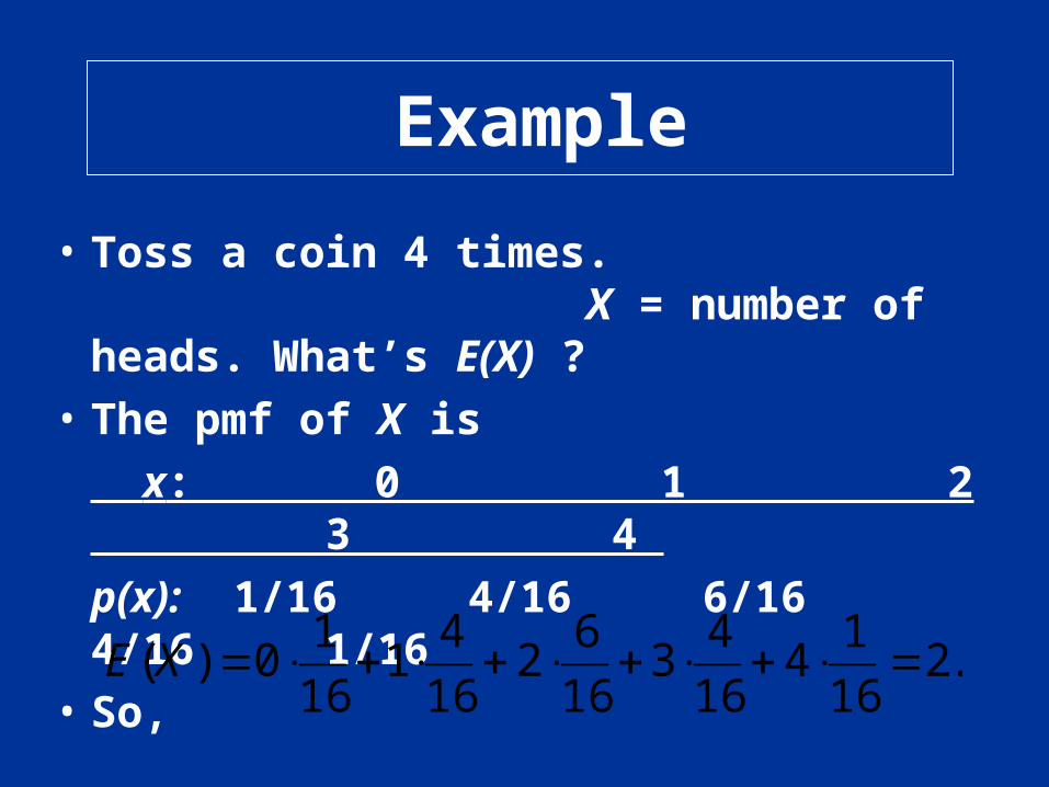
• Toss a coin 4 times. X = number of heads. What’s E(X) ?
• The pmf of X is
x: 0 1 2 3 4
p(x): 1/16 4/16 6/16 4/16 1/16
• So,
.216
14
16
43
16
62
16
41
16
10)( XE

Example
• Let X be a Bernoulli rv with pmf
Then E(X) = 0p(0) + 1p(1) = p. So the expected value of X is just the probability that X takes on the value 1.
1
0 1)(
xp
xpxp
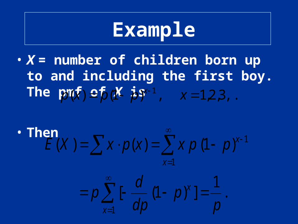
Example• X = number of children born up to and
including the first boy. The pmf of X is
• Then
,...3,2,1 ,)1()( 1 xppxp x
.1
])1( [
)1( )()(
1
1
1
pp
dp
dp
ppxxpxXE
x
x
x
x
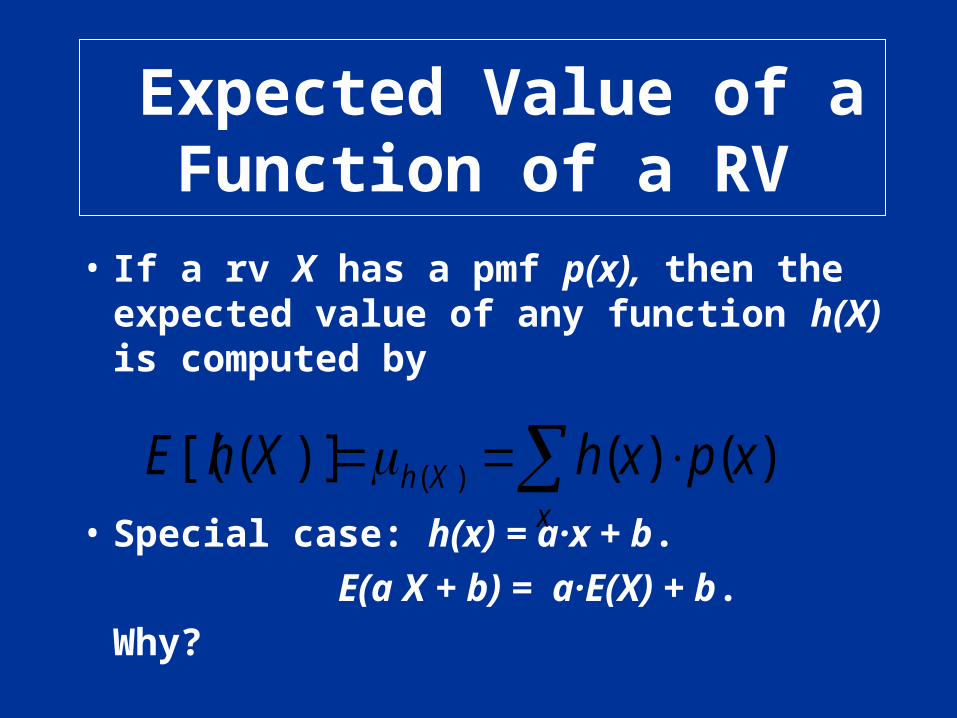
Expected Value of a Function of a RV
• If a rv X has a pmf p(x), then the expected value of any function h(X) is computed by
• Special case: h(x) = a·x + b. E(a X + b) = a·E(X) + b. Why?
x
Xh xpxhXhE )()()]([( )(

Variance
• The expected value measures the center of a probability distribution.
• Variance measures the variability of a pmf.
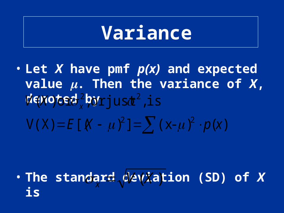
Variance
• Let X have pmf p(x) and expected value . Then the variance of X, denoted by
• The standard deviation (SD) of X is
).()-(x ])[( V(X)
is ,just or ,or )(22
22
xpXE
XV x
).(XVx

Example
• If X has pmf :
x 1 2 6 8
p(x) .4 .1 .3 .2
Then = 1×.4 + 2×.1 + 6×.3 + 8×.2 = 4 . 2 = (1 - 4)2×.4 + (2 - 4)2 × .1 + (6 - 4)2 ×.3
+ (8 - 4)2 ×.2 = 8.4.
and = 2.90.
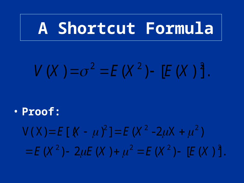
A Shortcut Formula
• Proof:
.)]([)()( 222 XEXEXV
.)]([)()(2)(
) X2-(])[( V(X)2222
222
XEXEXEXE
XEXE
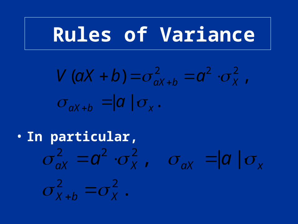
Rules of Variance
• In particular,
.||
,)(
222
xbaX
XbaX
a
abaXV
.
|| ,22
222
XbX
xaXXaX aa
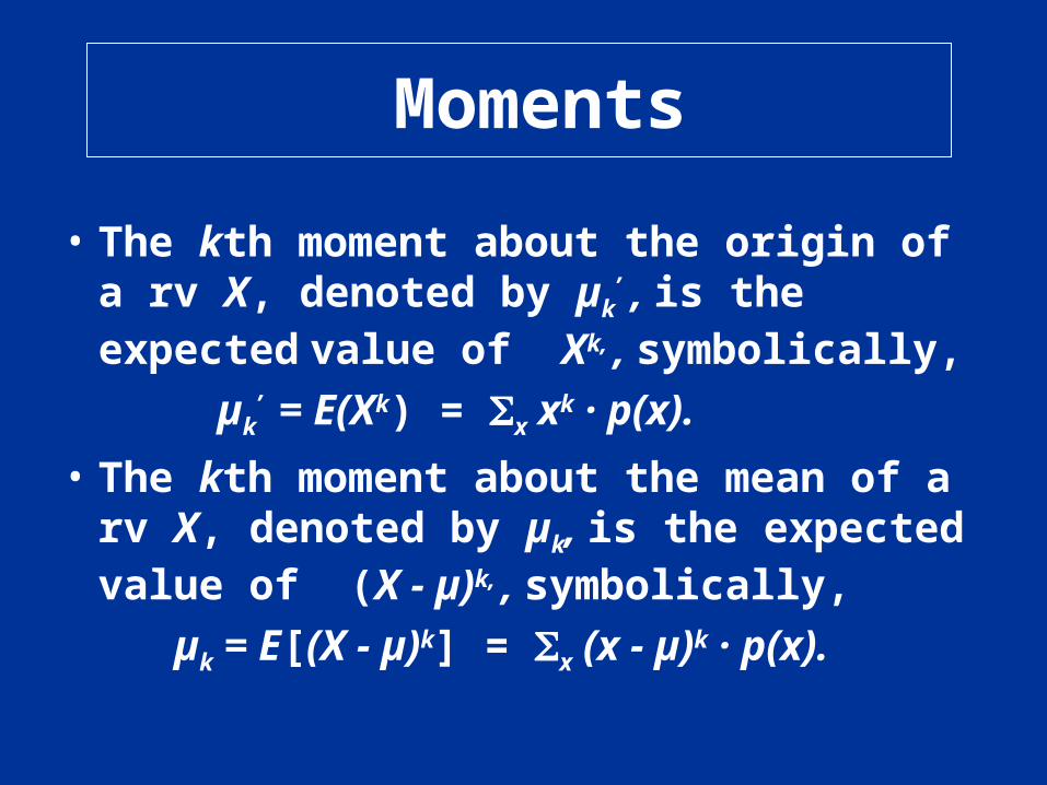
Moments
• The kth moment about the origin of a rv X, denoted by µk
’ , is the expected value of Xk, , symbolically,
µk’ = E(Xk) = x xk · p(x).
• The kth moment about the mean of a rv X, denoted by µk, is the expected value of (X - µ)k, , symbolically,
µk = E[(X - µ)k] = x (x - µ)k · p(x).

Special Cases
• The expectation, or the mean, is the 1st moment about the origin.
µ = µ1’ = E(X) = x x · p(x).
• The variance is the 2nd moment about the mean
2 = µ2 = E[(X - µ)2] = x (x - µ)2 · p(x).

The Binomial Distribution
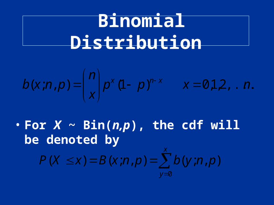
Binomial Distribution
• For X ~ Bin(n,p), the cdf will be denoted by
.,...,2,1,0 )1(),;( nxppx
npnxb xnx
x
y
pnybpnxBxXP0
),;(),;()(
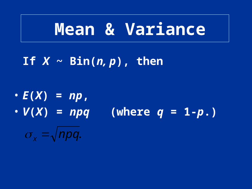
Mean & Variance
If X ~ Bin(n, p), then
• E(X) = np,
• V(X) = npq (where q = 1-p.)
.npqx

Example(Cont)
• n = 5, p = 11/32 . Then
• E(X) = n · p = 5 · 11/32 = 1.72.
• V(X) = n · p · q = 5 · 11/32 · 21/32 = 1.13. = (1.13)1/2 = 1.06.

Hypergeometric and Negative Binomial
Distribution
Introduction
• The hypergeometric and negative binomial distribution are both closely related to the binomial distribution.
Introduction
• The negative binomial distribution arises from fixing the number of S’s and letting the number of trials to be random.
• The hypergeometric distribution is the exact probability model for sampling without replacement from a finite dichotomous (S,F) population.
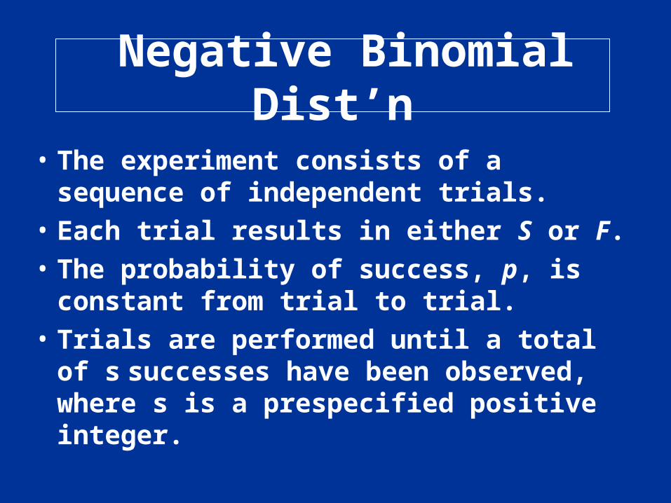
Negative Binomial Dist’n
• The experiment consists of a sequence of independent trials.
• Each trial results in either S or F.
• The probability of success, p, is constant from trial to trial.
• Trials are performed until a total of s successes have been observed, where s is a prespecified positive integer.
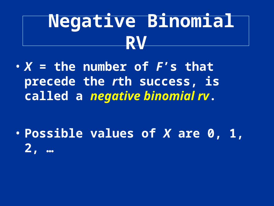
Negative Binomial RV
• X = the number of F’s that precede the rth success, is called a negative binomial rv.
• Possible values of X are 0, 1, 2, …

pmf
• Denote by nb(x; r, p) the pmf of X. Then
• Why?
• Total # of trials = x; The last trial must be a success. Among the first (x-1) trials, there are (s - 1) successes & x-s failures.
,...2,1 ,)1(1
1),;(
xpps
xpsxnb sxs
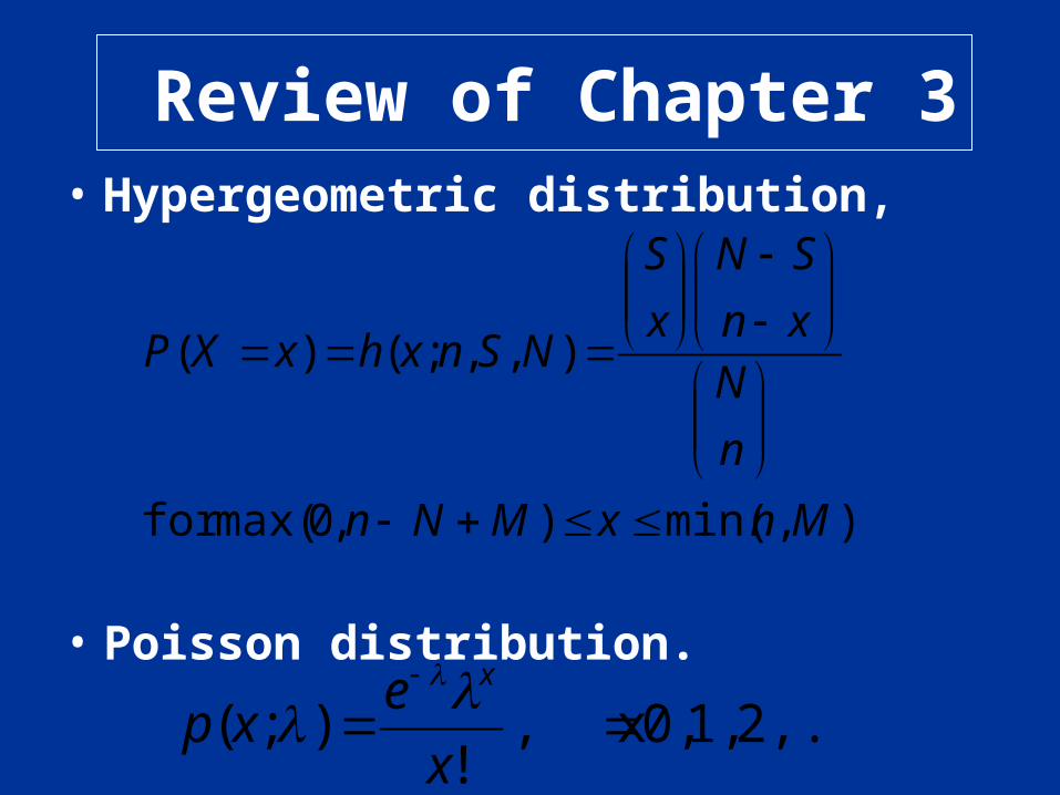
Review of Chapter 3• Hypergeometric distribution,
• Poisson distribution.
2,... 1, 0, x,!
);(
x
exp
x
).,min(),0max(for
),,;()(
MnxMNn
n
Nxn
SN
x
S
NSnxhxXP

Example
• What’s the probability that < 3 requests are received during a particular hour?
• P( X < 3) = P(0) + P(1) + P(2)
= e-5 + 5· e-5 + 52 · e-5/2
= 0.125.
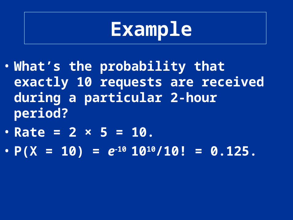
Example
• What’s the probability that exactly 10 requests are received during a particular 2-hour period?
• Rate = 2 × 5 = 10.
• P(X = 10) = e-10 1010/10! = 0.125.
Example
• How many calls do they expect to get during a 45-min period?
• E(X) = (3/4) · 5 = 3.75.

Continuous RVs&
Probability Distributions
Continuous RV
• An rv X is continuous if its set of possible values is an entire interval of numbers.
Example:
• X = the pH of a random soil sample
• X = the weight of a randomly selected
person.

• Let X be a continuous rv. Then a probability density function (pdf) of X is a function f(x) such that for any two numbers a and b with a b,
• For f(x) to be a pdf, f(x) must satisfy:
f(x) 0 for all x, and
b
adxxfbXaP .)()(
.1)(
dxxf
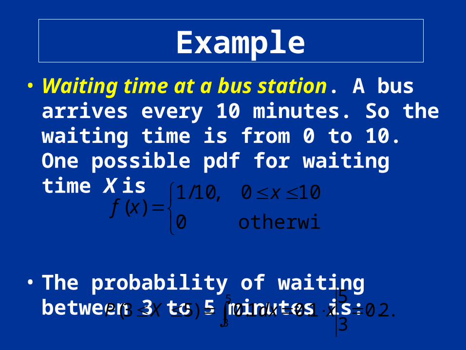
Example• Waiting time at a bus station. A bus
arrives every 10 minutes. So the waiting time is from 0 to 10. One possible pdf for waiting time X is
• The probability of waiting between 3 to 5 minutes is:
otherwise. 0
100 ,10/1)(
xxf
.2.03
5 1.0 1.0)53(
5
3 xdxXP

Uniform Distribution
• A continuous rv X is said to have a uniform distribution on the interval [A, B] if the pdf of X is
• Graphs of uniform distributions.
otherwise 0
)/(1) , ;(
BxAABBAxf

Probability at a Point
• When X is a discrete rv, each possible value is assigned positive probability. This is no longer true for continuous rv.
• If X is a continuous rv, then for any number c, P(X = c) = 0. Consequently, P(a X b) = P(a < X b) = P(a X < b)
= P(a < X < b).
Example
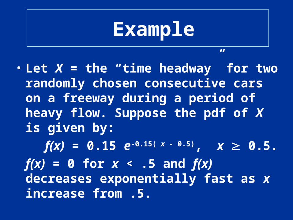
• Let X = the “time headway” for two randomly chosen consecutive cars on a freeway during a period of heavy flow. Suppose the pdf of X is given by:
f(x) = 0.15 e-0.15( x - 0.5), x 0.5.
f(x) = 0 for x < .5 and f(x) decreases exponentially fast as x increase from .5.
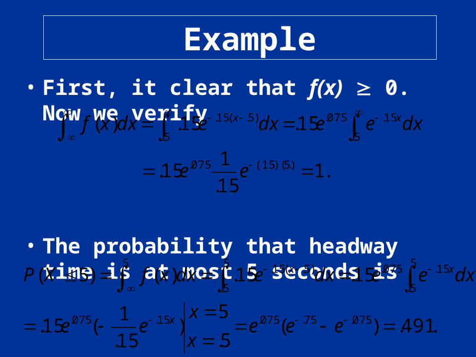
Example• First, it clear that f(x) 0. Now we verify
• The probability that headway time is at most 5 seconds is
.115.
115.
15.15.)(
)5)(.15(.075.
5.
15.075.
5.
)5.(15.
ee
dxeedxedxxf xx
.491.)(5.
5)
15.
1(15.
15.15.)()5(
075.75.075.15.075.
5
5.
15.075.5 5
5.
)5.(15.
eee
x
xee
dxeedxedxxfXP
x
xx

CDFs & Expected Values
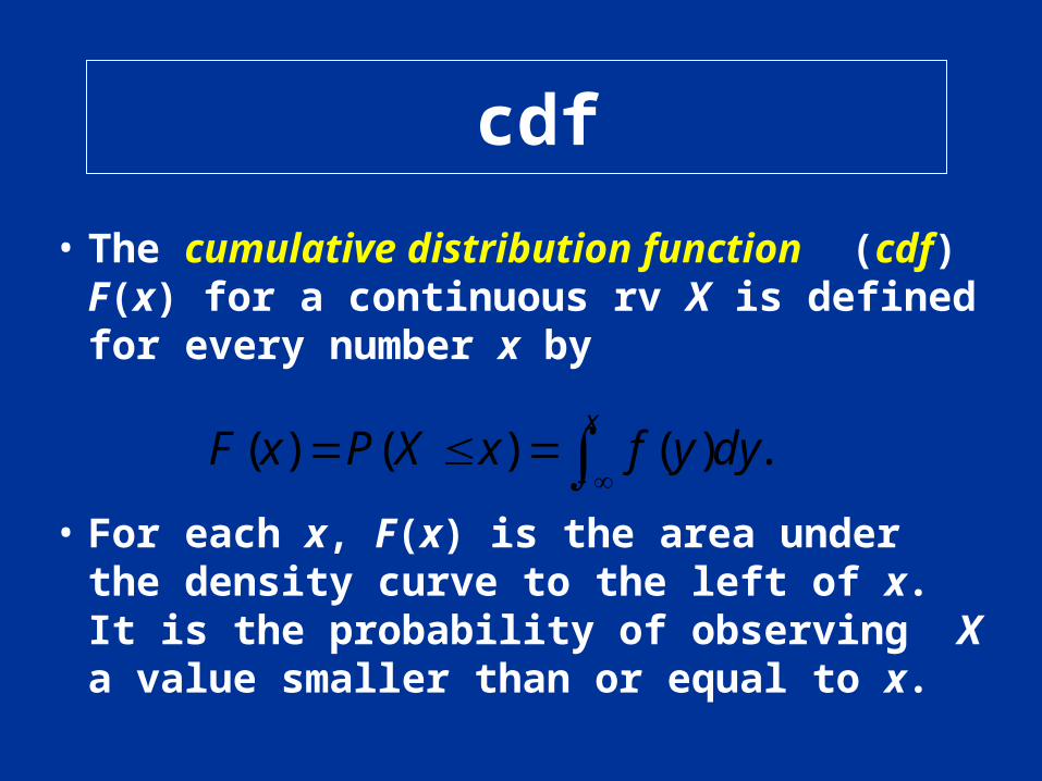
cdf
• The cumulative distribution function (cdf) F(x) for a continuous rv X is defined for every number x by
• For each x, F(x) is the area under the density curve to the left of x. It is the probability of observing X a value smaller than or equal to x.
xdyyfxXPxF .)()()(
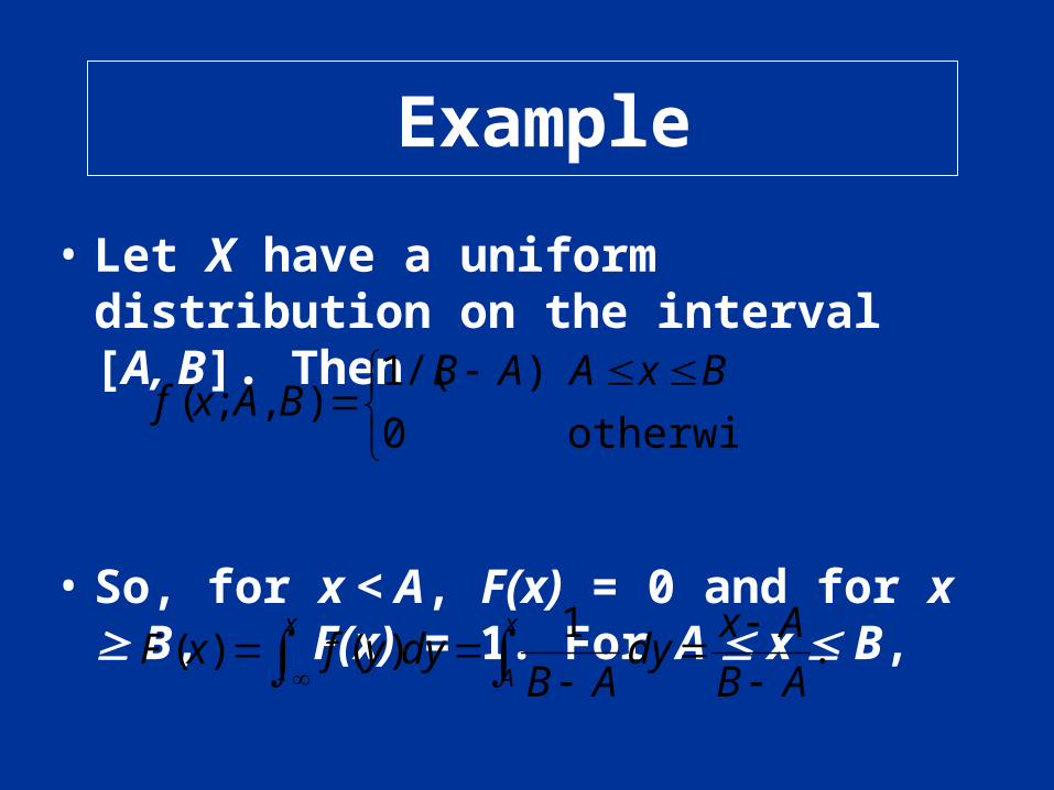
Example
• Let X have a uniform distribution on the interval [A, B]. Then
• So, for x < A, F(x) = 0 and for x B, F(x) = 1. For A x B,
otherwise 0
)/(1) , ;(
BxAABBAxf
.1
)()(
x x
A AB
Axdy
ABdyyfxF

Example
• The entire cdf is:
• The graph of the cdf looks like:
. 1
0
)(
Bx
BxAAB
AxAx
xF
Propositions
• Compute probabilities using F(x): P(a x b) = F(b) - F(a).
• Obtaining pdf from cdf:
• If X is a continuous rv with cdf F(x) differentiable at every point x, then the pdf f(x) =F ’(x).

Example
• For uniform distribution on [A, B], the cdf is
• So, for example, if A < a < b < B, then P(a < X < b) = F(b)-F(a) = (b-a)/(B-A).
• The pdf
• f(x) = F ’(x) = 1/(B-A) for A < x < B.
. 1
0
)(
Bx
BxAAB
AxAx
xF
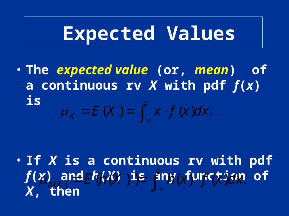
Expected Values
• The expected value (or, mean) of a continuous rv X with pdf f(x) is
• If X is a continuous rv with pdf f(x) and h(X) is any function of X, then
.)()( dxxfxXEX
.)()())(()( dxxfxhXhEXh
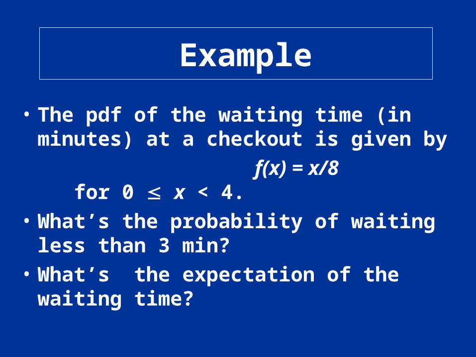
Example
• The pdf of the waiting time (in minutes) at a checkout is given by
f(x) = x/8 for 0 x < 4.
• What’s the probability of waiting less than 3 min?
• What’s the expectation of the waiting time?
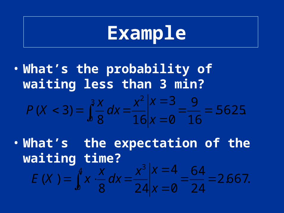
Example
• What’s the probability of waiting less than 3 min?
• What’s the expectation of the waiting time?
.5625.16
9
0
3
16
8)3(
23
0
x
xxdxx
XP
.667.224
64
0
4
24
8)(
34
0
x
xxdxx
xXE

Variance & S.D.
• The variance of a continuous rv X with pdf f(x) and mean is
• The standard deviation (S.D.) of X is
• V(X) = E(X2) - [E(X)]2.
].)[()()()( 222 xEdxxfxXVX
).(XVx

Linear Transformation
• If h(X) = a X + b and V(X) = 2, then
V(h(X))=V(a X + b) = a 2 2
and
aX+b = |a| .
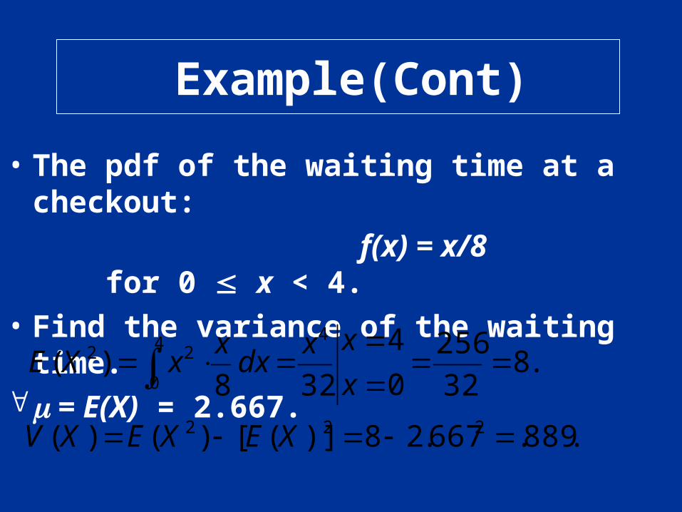
Example(Cont)
• The pdf of the waiting time at a checkout:
f(x) = x/8 for 0 x < 4.
• Find the variance of the waiting time. = E(X) = 2.667.
.889.667.28)]([)()(
.832
256
0
4
32
8)(
222
44
0
22
XEXEXV
x
xxdxx
xXE

Normal Distribution

Introduction
• The normal distribution is the most important distribution in all of probability and statistics.
• Many numerical populations have distributions that can be approximated very well by a normal curve.
Example
• Scores of standardized tests,
• Measurements of intelligence & aptitude,
• Returns of a stock (or a portfolio),
• Measurement errors …
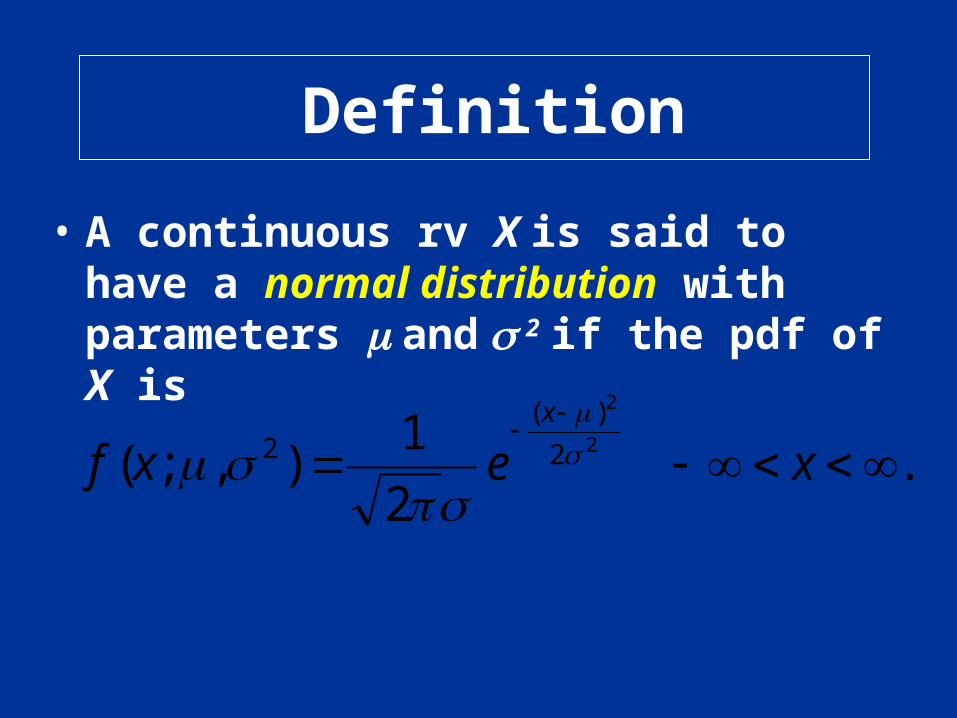
Definition
• A continuous rv X is said to have a normal distribution with parameters and 2 if the pdf of X is
. 2
1), ;(
2
2
2
)(2
xexfx
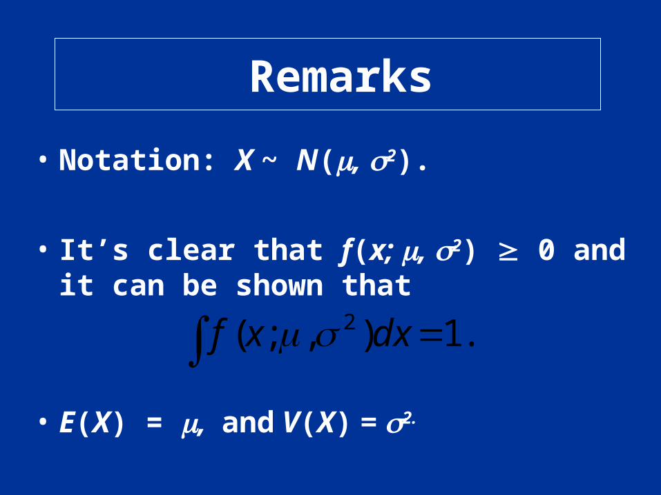
Remarks
• Notation: X ~ N(, 2).
• It’s clear that f(x; , 2) 0 and it can be shown that
• E(X) = , and V(X) = 2.
.1),;( 2 dxxf
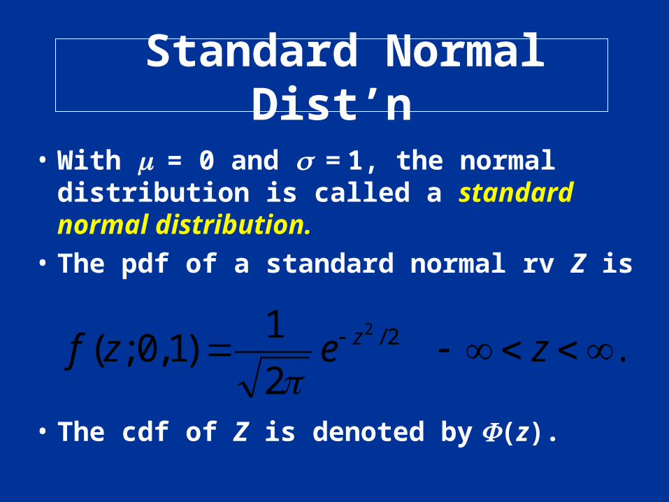
Standard Normal Dist’n
• With = 0 and = 1, the normal distribution is called a standard normal distribution.
• The pdf of a standard normal rv Z is
• The cdf of Z is denoted by (z).
. 2
1)1 ,0 ;( 2/2
zezf z
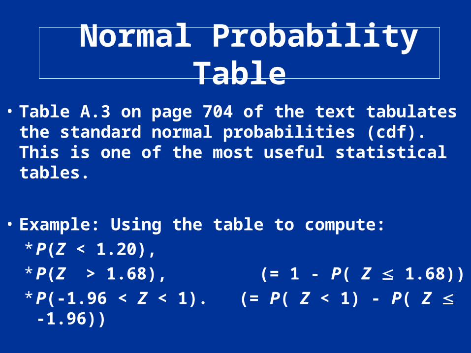
Normal Probability Table
• Table A.3 on page 704 of the text tabulates the standard normal probabilities (cdf). This is one of the most useful statistical tables.
• Example: Using the table to compute:* P(Z < 1.20), * P(Z > 1.68), (= 1 - P( Z 1.68)) * P(-1.96 < Z < 1). (= P( Z < 1) - P( Z -1.96))
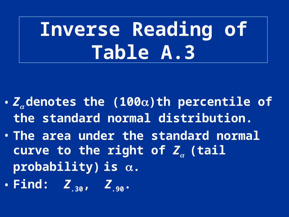
Inverse Reading of Table A.3
• Z denotes the (100)th percentile of the standard normal distribution.
• The area under the standard normal curve to the right of Z (tail probability) is .
• Find: Z.30, Z.90.

Standardization
• If Z ~ N(0, 1), then X = + Z ~ N(, 2).
• Inversely, if X ~ N(, 2), then
Z = (X - )/ ~ N(0, 1).
• The transformation
Is called standardization.
• P(X x) =P[Z (x - )/] = [(x - )/].
X
ZX
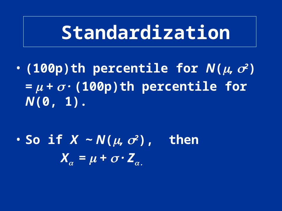
Standardization
• (100p)th percentile for N(, 2)
= + · (100p)th percentile for N(0, 1).
• So if X ~ N(, 2), then
X = + · Z .
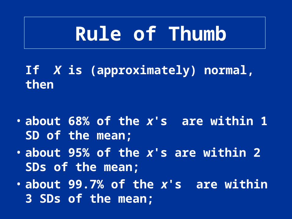
Rule of Thumb
If X is (approximately) normal, then
• about 68% of the x's are within 1 SD of the mean;
• about 95% of the x's are within 2 SDs of the mean;
• about 99.7% of the x's are within 3 SDs of the mean;

Example(Fish)
The lengths of fish in a certain fish population follows a normal distribution with = 54 mm and = 4.5 mm.
• What percentage of the fish are between 50 and 60 mm long?
* Let Z = (X - )/. Then
z1=(50 - 54)/4.5= -.89, z2=(60 - 54)/4.5=1.33.
Use Table A.3: P(50 X 60)=P(-.89Z1.33) =.9082- .1867 = .7215.
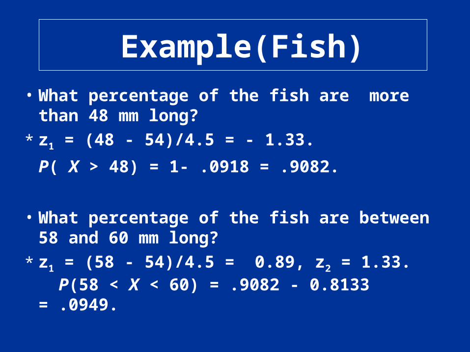
Example(Fish)
• What percentage of the fish are more than 48 mm long?
* z1 = (48 - 54)/4.5 = - 1.33.
P( X > 48) = 1- .0918 = .9082.
• What percentage of the fish are between 58 and 60 mm long?
* z1 = (58 - 54)/4.5 = 0.89, z2 = 1.33. P(58 < X < 60) = .9082 - 0.8133 = .0949.

Example(Fish)
• What is the 70th percentile of the fish length ? What is the 90th percentile?
* From Table A.3, Z.70 = 0.52. So, X.70 = 54 + 4.5 ·0.52 = 56.3
* Similarly, Z.90 = 1.29. and
X.90 = 54 + 4.5 ·1.29 = 59.80.
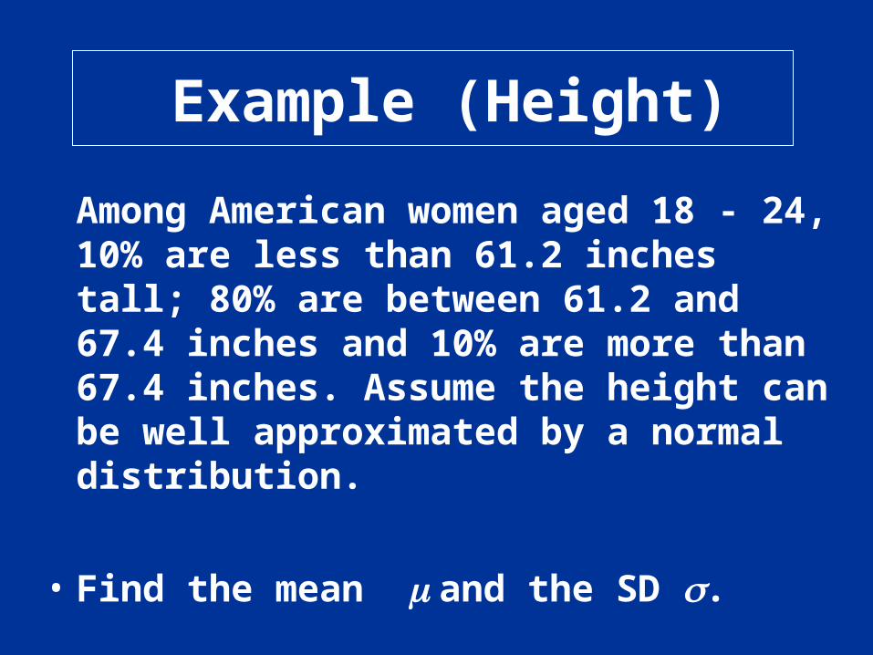
Example (Height)
Among American women aged 18 - 24, 10% are less than 61.2 inches tall; 80% are between 61.2 and 67.4 inches and 10% are more than 67.4 inches. Assume the height can be well approximated by a normal distribution.
• Find the mean and the SD .
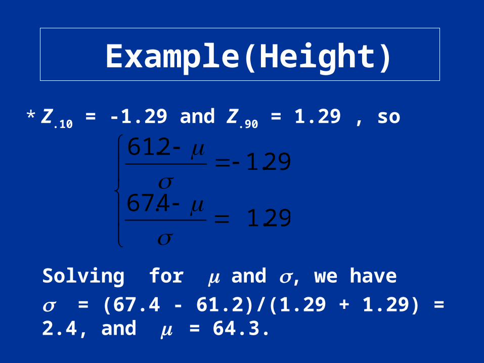
Example(Height)
* Z.10 = -1.29 and Z.90 = 1.29 , so
Solving for and , we have = (67.4 - 61.2)/(1.29 + 1.29) = 2.4, and
= 64.3.
29.1 4.67
29.12.61

Normal Approximation
• The normal distribution is often used to approximate the distribution of discrete populations.
• In particular, under certain conditions, the normal distribution can be used as an approximation to the binomial distribution.
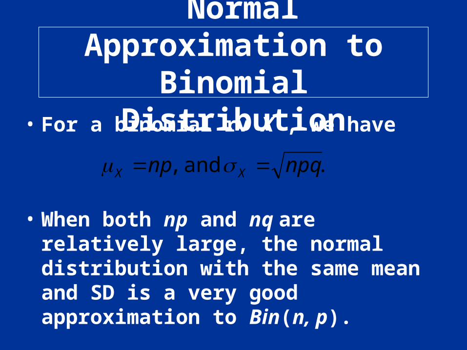
Normal Approximation to Binomial Distribution
• For a binomial rv X , we have
• When both np and nq are relatively large, the normal distribution with the same mean and SD is a very good approximation to Bin(n, p).
. and , npqnp XX

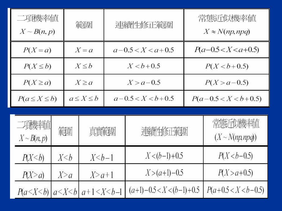
Normal Approximation to Binomial Distribution
• Let X ~ Bin(n, p), Then if np 5 and nq 5, X has approximately a normal distribution with
• This is the area under the normal curve to the left of x+.5. “+.5” is the correction for discreteness. This is called continuity correction.
. and , npqnp XX
).5.
(),;()(npq
npxpnxBxXP

Example • X ~ Bin(30, 0.3). Want: P(6 X 10).
• Mean=30 × .3 = 9, SD = (30× .3× .7)1/2=2.51.
• P(6 X 10) = P(X 10) - P(X 5) ((10 + .5 - 9)/2.51) - ((5 + .5 - 9)/2.51)
= (.598) - (-1.394)= .7257 - .0832= .6425.
• Direct calculation yields
P(6 X 10) = P(6) + … + P(10) = .6437.
• The results are very close.


