Review Impedance spectroscopy of interfaces, membranes …ucanr.edu/datastoreFiles/608-554.pdf ·...

Bioelectrochemistry and Bioenergetics 40 (1996) 79-98

Review

Impedance spectroscopy of interfaces, membranes and ultrastructures

Hans G.L. Coster * , Terry C. Chilcott, Adelle CF. Coster UNESCO Centre for Membrane Science and Technology and Department of Biophysics, School of Physrcs. Unrversrty of New South Wales, Sydney 2052.

Australia

Received 26 January 1996; accepted 26 February 1996

Abstract

For the past century, impedance spectroscopy has provided a non-invasive means of characterizing the electrical properties of many systems. Even today, it often provides the only non-invasive method for detailed structural-functional studies of these systems. This is especially so of systems in which important processes occur at the molecular level, such as those processes associated with biological and synthetic membranes and interfaces that form between solutions and various solids (e.g. metals and colloid particles).

The fundamental concepts of impedance spectroscopy are re-examined and a review is given of the role that impedance spectroscopy has played in the development of our understanding of cellular and synthetic membranes, cell biophysics and ionic systems in general. Special emphasis is given to the problems associated with solution-electrode interfaces, as well as unstirred layers, which can plague measurements on biological systems and have led to much confusion in the past.

A description is given of a new computer-controlled, four-terminal digital impedance spectrometer, which provides resolutions in impedance magnitude and phase of 0.002% and 0.001” respectively over a frequency range of lo-* to lo5 Hz and for impedances ranging from 10 to 10’ a.

We also describe impedance dispersions in terms of transfer functions which, when plotted along the negative frequency axis, yield “spectra” with distinct sharp peaks that identify fundamental frequency constants of the system. This “control engineering” form of presentation of impedance spectra demystifies the impedance analyses of these systems. The spectra and changes in these which occur as a result of perturbations to the system can he readily assessed and interpreted.

Keywords: Impedance spectroscopy; Interfaces; Membranes: Ultrastructures

1. Introduction

Impedance measurements [ 1 I provided initial evidence of notions developed in the last century [2] that living cells were contained by a membrane with a low permeability to ions [3]. It is significant that, in 1925, impedance measurements also provided the first estimate of the thickness of a cell membrane [4], and yielded a value which was very clase to that determined some three decades later using electron microscopy [S].

Although electron microscopy was successfully used to image liposomes composed of bilayer membranes of lipid purified from biological membranes, estimates of the thickness of these membranes were first obtained from impedance measurements of a single planar bilayer [6]. Subsequently, low-frequency impedance spectroscopy studies [7,8] probed the submolecular domains of such

* Corresponding author.

bilayers and achieved spatial resolutions of the order of 0.1 nm. Even now, electron microscopy and X-ray crystal- lographic studies of isolated protein purified from biological membranes have not been able to match the spatial resolutions achieved with impedance spectroscopy. The implication is that impedance studies of bilayers consisting of purified lipid and protein have an important role to play in elucidating the various mechanisms of transport [9] that have been attributed to specific proteins of biological membranes.

Of simiIar importance are the special electrochemical processes that only occur within the molecular dimensions of interfaces formed between solids and solutions. The mechanisms whereby such interfaces facilitate these processes remain unresolved.

Impedance studies of processes associated with membranes and solids immersed in solutions [ IO,1 I] are of fundamental importance to the interpretation of impedance measurements of more complex biological systems, such

0302-4598/%/$15.00 Copyright 0 1996 Elsevier Science S.A. AH rights reserved. PII SO302-4598(96)05064-7

80 H.G.L. Caster et al./ Bioclectrochemistry and Bioenergetics 40 (1996) 79-98

as single cells [12], tight epithelium of the bladder [13], striated muscle fibres [14] and even the human thorax [15] and breast [16]. This is also true of synthetic separation systems involving ultrafiltration membranes. Inevitably solid-solution interfaces develop in these systems, even if only as a consequence of the impedance electrodes making contact with the aqueous phases.

2. Impedance spectroscopy

2.1. Fundamentals

Impedance measurements are made by applying a small alternating (a.c.> current of known frequency w and small amplitude i, to a system and measuring the amplitude ua and phase difference $ of the concomitant electrical potential that develops across it. Impedance is usually represented by a phasor, the magnitude and phase of which are given by

]Z]=; and LZ=4 (1)

In Cartesian coordinates, impedance becomes a complex number

Z=R+jX where j=\r_l (2)

The real and imaginary parts of Z describe the resistance (R) and reactance (X) respectively and can be represented by appropriate electrical circuit elements in series.

It should be noted here that impedance is only a specific form of the transfer function of the system. Thus if fls] and v[ S] denote the well-known Laplace transforms of the sinusoidal functions describing the a.c. current and electrical potential respectively, the transfer function is

WI uo l-F(s)--=- ITS] io (

cos 4 + ” sin 4 6J 1

(3)

where s is the Laplace complex variable or frequency. If s=jo, then solutions to Eq. (3) are confined to the frequency domain. This restriction leads directly to the same definition of impedance given by Eq. (2)

Z=7F(jw)=$cos#+jzsin+

2.2. Why vary the frequency?

The impedance of a homogeneous material may be expressed in terms of a conductance element G in parallel with a capacitance element C, thus

1 Z(w) =

G+jwC (5)

Although G and C are, individually, constant in frequency, it is immediately plain that the impedance, expressed in this manner, will disperse with frequency.

The parameters G and C describe the ability of the homogeneous material to conduct and store electric charge respectively. For a slab of cross-sectional area A and thickness x, these properties are given by

(6)

where the constants cr and E are the electrical conductivity and dielectric permittivity of the material respectively.

Therefore an impedance measurement of this simplest of systems provides estimates of

G=Lcos$ and c= - 1

IZI - sin $ 44 (7)

for the slab and therefore its thickness via Eq. (6). Inspec- tion of Eq. (5) reveals that the dispersion becomes most pronounced for frequencies greater than G/C, with

G f&c--

C (8)

describing the condition for which the impedance measurement provides the most accurate estimates of both properties (see the dispersion of IZI in Fig. l(A)). This condition also happens to define the “natural” or characteristic frequency of this homogeneous system.

A heterogeneous system can be represented by a number of different materials or slabs sandwiched together, the total impedance of which is given by

Z,(w)= i l

n= I G, +.bC,,

(9)

where the subscript “~1” identifies the conductances and capacitances of each of the slabs. The dispersion described by Eq. (9) comprises N superimposed dispersions of the type described by Eq. (51, each of which commences near its respective “natural” frequency, i.e.

Gn w, z - cn

(10)

If these and the magnitudes of the corresponding N impedance dispersions are sufficiently different, each impedance dispersion can be immediately identified within the combined impedance dispersions. More often, however, the situation depicted in Fig. l(A) is encountered, where dispersions of the impedance magnitude for the system consisting of two slabs are indistinguishable from those for the system consisting of one slab. This illustrates that the presence of more than one characteristic frequency cannot be so readily discerned from the dispersion of the impedance magnitude alone. To detect the presence of the second slab requires a knowledge of the dispersion of the impedance phase (see Fig. l(B)). In fact, mathematical

H.G.L. Caster et al. / Bioelectrochemistry and Bioenergetics 40 (1996) 79-98 81

algorithms [17] have been devised for separating such substructural contributions from measured impedance dispersions of both the magnitude and phase.

2.3. Dispersions of conductance and capacitance

In the simple multilayered systems referred to thus far, it is often convenient to describe and present the impedance in terms of the overall parallel conductance G(w) and capacitance C(o) at a particular 0. Then

1 Z(w) =

G( co) +j,C( LO) (11)

A

0 1 F& / :,"d s-1

loo0 loo00

f% B lco.0

80.0

I e!

60.0

P P

ii

E 40.0

20.0

0.0 i

I-JL-Ii-JL-I

Fig. 1. Impedance dispersions with frequency for a single-layer ( -) and two-layer (-----I system. The equivalent circuits for the systems are shown in the insets. It should be noted that the dispersions of the impedance magnitudes (A) for the two systems are indistinguishable, whereas those for the impedance phases (B) differ slightly in the frequency range lo-lo3 rad.s- ‘. On the basis of the impedance magnitude, it is not possible to detect the additional layer present in the two-layer system.

5.4 I I I,,,,,, I I I ““‘, I I I ““,, I I , ,,q

1 10 Freqw$ /rod s-1

1OM loo00

0.04

1

.----. c ,

, , G,

, ,-\/ml-, ,-$L,

0.03

0.02

0.01

, I

1 10 100 IOCO loo00

Frequency / rad s-i

Fig. 2. The conductance and capacitance of the single-layer (- ) and two-layer (- - -1 system shown in Fig. I. The conductance and capacitance for the single-layer system are constant in frequency, whereas those of the two-layer system disperse very strongly with frequency. Generally, the range of frequencies over which the dispersion occurs tends to become wider as additional layers are introduced into the system.

For a single slab (i.e. N = l), equating Eq. (9) and Eq. (11) yields

G(w)=G, and C(o)=C, (12) i.e. conduction and capacitive properties that are constant in o, as shown in Fig. 2 for N = 1. However, for a sandwich of two or more slabs (i.e. N > 21, these properties disperse with frequency, as shown in Fig. 2 for N = 2. The dispersions for the two-slab system are

G(o)= G,G,(G, + G2) + o’(G,C; + G2C:)

(G, + G,)* + a~*( C, + C,)* (13)

C(w)= w2C,C2( C, + C,) + (C,G; + C,G:)

(G,+G2)2+w2(C,+C2)2 (14)

82 H.G.L. Caster et al./ Bioelectrochemistry and Bioenergetics 40 11996) 79-98

where the subscripts ‘* 1” and “2” identify the frequency- independent properties of each slab. With increasing numbers of slabs, these dispersions extend over a wider range of frequencies. Furthermore, the form of the dispersion curves becomes dependent on N. In contrast, the dispersions of the impedance magnitude are largely unaltered by N (cf. Fig. 1 and Fig. 2). Thus dispersions of the conductance and capacitance provide an immediate indication of the presence of substructure within the system.

A further comparison of Fig. 1 and Fig. 2 emphasizes the importance of measuring both the magnitude and phase of the impedance. Accurate measurements of the phase at each frequency enable the conductance and capacitance to be determined at each frequency (e.g. see Eq. (7)); it is the dispersions in G(o) and C(w) which so dramatically reveal the individual contributions from the different materials that constitute the system. Measurements of the dispersion of the impedance magnitude alone cannot generally be made with sufficient precision to discern the presence of substructure of biophysical interest.

2.4. Complex conductivity and complex relative permittivity

Rearrangement of Eq. (11) yields the general expression for the admittance of a heterogeneous system

Y(w) = &=G(w)+jwC(w)=;

which, for an area A and thickness x yields

Y(w)=~[o-(w)+jws(w)l=~ (16)

via definitions that normally apply to homogeneous materials (Eq. (6)). Using the definitions for current density and electric field

&; md E=-! X

which apply for a planar geometry, a definition of the complex conductivity of the material, i.e.

j u *=-= --

E a(w) +jws(o) (18)

follows. Equivalently, when the complex capacitance is defined as

c* E Y(o) A

I

44 -=- c((&)-j- jo x w I

(19)

this leads to the definition for the complex relative permittivity (or complex dielectric constant)

* _ 44 44 & =-- ‘- J E E’ - j,'

CO W&O

where cO is the permittivity of free space.

3. The origins of impedance dispersion in ionic diffusion systems

Impedance dispersions in biological systems arise from a variety of sources. In biological tissue, three distinctive relative permittivity (E) dispersions, labelled (Y, B and y in Fig. 3, have been broadly identified with specific frequency ranges and dispersion mechanisms [ 183.

In order to explain these mechanisms, it is useful to consider the Nemst-Planck-Poisson [ 191 electrodiffusion equations for ions in an electrolyte containing two univa- lent species of opposite charge.

3.1. The Nernst-Planck-Poisson electrodiffusion theory

We denote the steady state concentrations of positive and negative ions by P and N respectively, and the a.c. perturbations of these concentrations by the respective lower case characters, p and n. The Nemst-Planck equation then yields the following expression for the a.c. current density J at a position x

where E represents the steady state electric field and E” represents the a.c. perturbation of the field (k is the Boltzmann constant and T is the temperature). For a system in which there may be fixed charges F *, the steady state and a.c. forms of Poisson’s equation are

dE -= dX

-%(N-P-F*) and z= -:(n-p)

(22)

The effects of diffusion are represented by the first term in Eq. (21), which is the product of the electronic charge

I b lo2 IO' 1O'O

Frequency

Fig. 3. A schematic illustration of the three major regions (a, p. y) in the dispersions of the relative dielectric permittivity with frequency found in biological tissue.

H.G.L. Caster er ul. /Bioelecrrochrmi.stry ond Bioenergetics 40 (1996) 79-98 83

(q), the diffusion constant (0) and the gradients in the a.c. concentration of the positive and negative ions.

For positions remote from membranes and electrode interfaces, where there are no fixed charges (F * = O), the conditions N = P and n = p hold to a good approxima- tion. Eq. (22) then yields a steady state and an a.c. electric field which are constant in x and gradients that are the same for both positive and negative ions. Thus, in the bulk phases of the solution, the effects of diffusion on the a.c. impedance are negligible.

If no steady electric field is applied (i.e. E = O), the second term, which represents the drift current, is also negligible. Thus, for a homogeneous electrolyte system alone, we have from Eq. (21)

J q2Dbulk -- --(P+N) +jmbulk Ebulk

(23)

which yields the same form of complex conductivity as Eq. (18). Thus the specific intrinsic conductance of the system is

ub*ulk = (Tbulk + hEbulk

where

3.2. The (Y dispersion

The CY dispersion occurs as a consequence of the frequency dependence of the relative magnitudes of the a.c. diffusion and a.c. field-driven currents in the a.c. Nernst- Planck equation (the first two ’ terms in Eq. (21) relative to the last term). An a.c. electric field (.!?> of low frequency will establish (a.c.) ionic concentrations and gradients, which will generally be different for positive and negative ions. Such conditions yield diffusion currents that can be significantly larger than the field-driven current (i.e. the last term in Eq. (21)). Since the former current involves the establishment of (a.c.) ionic concentrations and gradients, they will be out of phase with ,l? and, conse- quently, will lead to impedances with characteristics similar to those of very large capacitors. For increasing frequencies (approaching 100 Hz for biological systems), the time available in each half a.c. cycle for the establishment of a.c. ionic concentrations and gradients diminishes, and the a.c. diffusion currents then become negligible com- pared with the a.c. field-driven term. This leads to a decrease in the reactive component (capacitance) of the impedance as the frequency increases.

Beyond the c1 dispersion, the bulk (intrinsic) electrical properties pertain for each component of the system (electrolyte, membrane, etc.). Thus, for each component, we can identify a complex conductance

u * = afj6x (25) which derives from the a.c. field-driven current in the a.c. Nemst-Planck equation.

When a permeable membrane with a high concentration of fixed charges (F * # 0) is immersed in an electrolyte, the steady concentration of those ions with opposite charge to that of the fixed charges (counter-ions) will be larger than, and independent ’ of, the bulk electrolyte values. On the other hand, the co-ion concentrations will be much smaller than the bulk electrolyte values. The conductance of the fixed charge membrane is determined by the steady concentrations of counter-ions and is given by

q*D u~-F+ kT

which is independent of the concentration of the electrolyte. For the interface regions between the membrane and the bulk solution, the ionic concentrations and gradients will be different for anions and cations. This will lead to conditions 3 (determined by the second term in JZq. (21)) which will produce an (Y dispersion at low frequency.

As the 0: dispersion is intimately connected with diffusion terms in the Nemst-Planck equation, the dispersion is characteristically temperature dependent. This is in contrast with the dispersion arising from, for instance, interfacial polarization which is discussed below.

3.3. The p dispersion: inteeacial polarization

When a system is composed of two or more layers or components, the total impedance of the system at frequencies above the CY dispersion can be determined from the intrinsic conduction and dielectric properties (i.e. complex conductance or complex dielectric constant) of the components making up the system. For our example of a biological membrane immersed in an electrolyte solution, Eq. (23) and Eq. (25) then yield the area-specific impedance of the system

Z,,,( w > 100Hz)

=

’ It should be noted that the second term in Eq. (21) is not necessarily zero when only an a.c. field is applied; in many cases (for instance, at the interface between a membrane or electrode and an electrolyte), the steady state concentrations of cations and anions are not equal (P Z N), and the steady electric field E will not always be zero, even when the steady applied field is zero.

*The condition for this is that yC, +z F, where y is the partition coefficient for ions between the bulk electrolyte and the membrane and C, is the concentration (P or N) of ions in the solution (see Ref. [20]).

3 Other properties, such as unequal ion partitioning into a membrane due to dielectric (Born energy) effects, can also give rise to these conditions (see also Section 4.3).

84 H.G.L. Coster et al. / Bioelectrochemistry and Bioenergetics 40 (1996) 79-98

which, using Eq. (61, can be identified as the type of dispersion described thus far by Eq. (9) and illustrated in Fig. 1 and Fig. 2. Such dispersions arise from polarization effects at the interface 4 between the bulk phases as a consequence of the boundary condition

&bulk 2 bulk = %em Rmil (28)

which the internal electric field must satisfy at the interfaces. These dispersions do not arise from within the bulk phases themselves, as the conductance and capacitance of each phase is constant in frequency (see Fig. 2).

3.4. The y dispersion: polar relaxation

Molecules which have a dipole moment will rotate in an a.c. electric field. Any induced net polarization effect arising from this will tend to be diminished by Brownian motion. This results in losses which give rise to a dispersion of the dielectric permittivity with frequency [21]. The characteristic frequencies of these dispersions decrease with increasing molecular size (and mass). Typically, for water and protein they are 20000 MHz and 1 MHz respectively. Since this review is concerned with impedance dispersions below 100 kHz, we refer readers to other sources for more comprehensive descriptions of polar relaxation and the y dispersion [22,23].

4. Examples in ionic and biophysical systems

4.1. The electrode-electrolyte interface

At a phase boundary between an electrolyte and the surface of an electrode, an electrochemical double layer is formed. It is the result of an unequal distribution of ions between the two phases. For instance, charges may diffuse from the electrode into solution, resulting in a surface with a net charge. This surface charge establishes an electric field which, in turn, modulates the ionic atmosphere about the surface. Ions in the solution are attracted and adsorbed to the surface. Further from this layer of adsorbed ions, the ions in the solution form a “diffuse layer” about the surface (see Fig. 4). The layer of charges at the surface and the diffuse layer in the solution together constitute what is termed the “double layer”.

Simple impedance models of this generally have the form of a resistance representing the solution in series with a capacitor representing the “double layer”, i.e.

Z=R-(jWC)-’ This is of course an oversimplification. For explicit impedance element should be added

(29) instance, an to take into

4 Hence the nomenclature: intcrfacial polarization.

I I Stern Gouy-Chapman Layer Layer

Fig. 4. Schematic representation of the electrode-electrolyte interface depicting the Stem layer and the Gouy-Chapman diffuse space charge region which extends from the Stem layer into the solution.

account the adhered layer of ions on the surface of the electrode, which is known as the “Stem” layer. The impedance of the whole system can be more accurately represented by a series combination of impedance elements representing each of the following regions: the Stem layer, the diffuse (Gouy-Chapman) double layer and the bulk solution (far from the electrode).

Impedance measurements made in our laboratory [24] of the gold-electrolyte interface at ultralow frequencies suggest that even this three-layer model is insufficient .to describe the impedance dispersion even qualitatively. A good fit to the data can be obtained if we introduce additional layers, i.e. additional elements with other characteristic frequencies. This is illustrated in Fig. 5, which shows the fit of Eq. (9) to the experimental conductance and capacitance dispersions obtained for the gold interface in a 10 mol me3 KC1 solution. This fit allows various elements to be assigned qualitatively to either the Gouy- Chapman or Stem layers on the basis of the characteristic frequencies (or time constants) of the elements. Such an assignment allows the thickness of the Stem layer to be estimated assuming a dielectric constant E N 5, a theoreti- cally expected value for this region due to dielectric saturation effects in the extremely high electric field which pertains therein (cf. Hasted et al. [25]). This yields a value of 0.27 nm for the thickness of the Stem layer, assuming that the topology of the metal surface at this scale of interest can be taken to consist of a mosaic of hemispheres corresponding to the gold atoms (as an initial approxima- tion of the roughness of the electrode surface, cf. Fig. 4). This estimate for the Stem layer thickness corresponds almost exactly to the diameter of a potassium ion.

The electrode-electrolyte polarization impedance for many electrode-electrolyte systems has been shown [26] experimentally to have the form

H.G.L. Cosrer et al./ Bioelectrochemistry and Bioenergetics 40 (1996) 79-98 85

1”

0.25

Frequency/Hz

Fig. 5. Dispersions of the conductance (A) and capacitance (B) with frequency for the gold electrode-electrolyt for a 10 mol m-3 KC1 solution. The vertical solid bars indicate the experimental data and error bars. The full line is a fit to the data, based on a seven-element Maxwell-Wagner model. The dispersion extends over a wide range of frequencies, indicating the presence of a range of time constants; the gold-electrolyte interface therefore cannot be simply modelled in terms of a combination of a Stem layer in series with a Gouy-Chapman diffuse layer.

where (Y is in the range O-l. A consequence of this fractional power relationship is that the polarization capacitance is an impedance element of constant phase angle. To account for this fractional power relation, it has been suggested [27-291 that the impedance dispersion arises from the effects of surface roughness. In this case, the electrode interface can be modelled using ladder networks of capacitors and resistors representing the branching impedance elements due to the solution in series with the local (Helmholtz) double layer [30,31].

Eq. (30) also implies that the double layer capacitance is necessarily frequency dependent. Precise measurements of the gold-KC1 interface at ultralow frequencies show that the dispersion in capacitance at very low frequencies is not consistent with that predicted 5 by Eq. (30) although the impedance magnitude follows this form closely. This emphasizes the requirement of an independent measurement of phase at low frequencies for distinguishing between impedance models.

5 Eq. (13) and EIq. (14) can bc used to calculate the equivalent frequency-dependent capacitance in a parallel configuration.

4.2. When intelfacial polarization effects between electrodes and solutions are a nuisance

Impedance measurements in membrane systems invari- ably involve the use of electrodes in contact with electrolyte solutions. However, as illustrated in Fig. 5, the impedances of the interfaces which form between these phases exhibit dispersions at frequencies which are also characteristic of membrane systems. For an accurate determination of the impedance of these systems, it is therefore important to be able to eliminate or, at the very least, identify the “nuisance” contributions arising from the complex impedance of the electrode-solution interface.

In principle, it is always possible to measure the interfacial electrode impedance separately and subtract it from the total to obtain an estimate of the system impedance. However, it has been shown that such estimates are thwarted by large experimental errors [32]. Since the subtraction involves complex quantities, very high accuracy is required for both the electrode and system + electrode measurements in order to minimize such errors.

One of the significant advantages introduced by the digital ultralow-frequency impedance technology described later is the capacity to perform four-terminal impedance measurements [33]. This technique utilizes a high-input impedance differential amplifier for sensing the electrical potentials of the system via electrodes separate from those used to inject the current (see also Fig. 15, Section 6). Thus electrical potentials which develop across the interfaces of the current injecting electrodes are simply not measured, and those which develop across the other interfaces can be neglected, since the amplifiers draw essentially zero current from the system. Four-terminal measurements therefore avoid measuring the impedance contributions from all the electrode-solution interfaces.

4.3. Unstirred layers at membrane-solution inte$aces

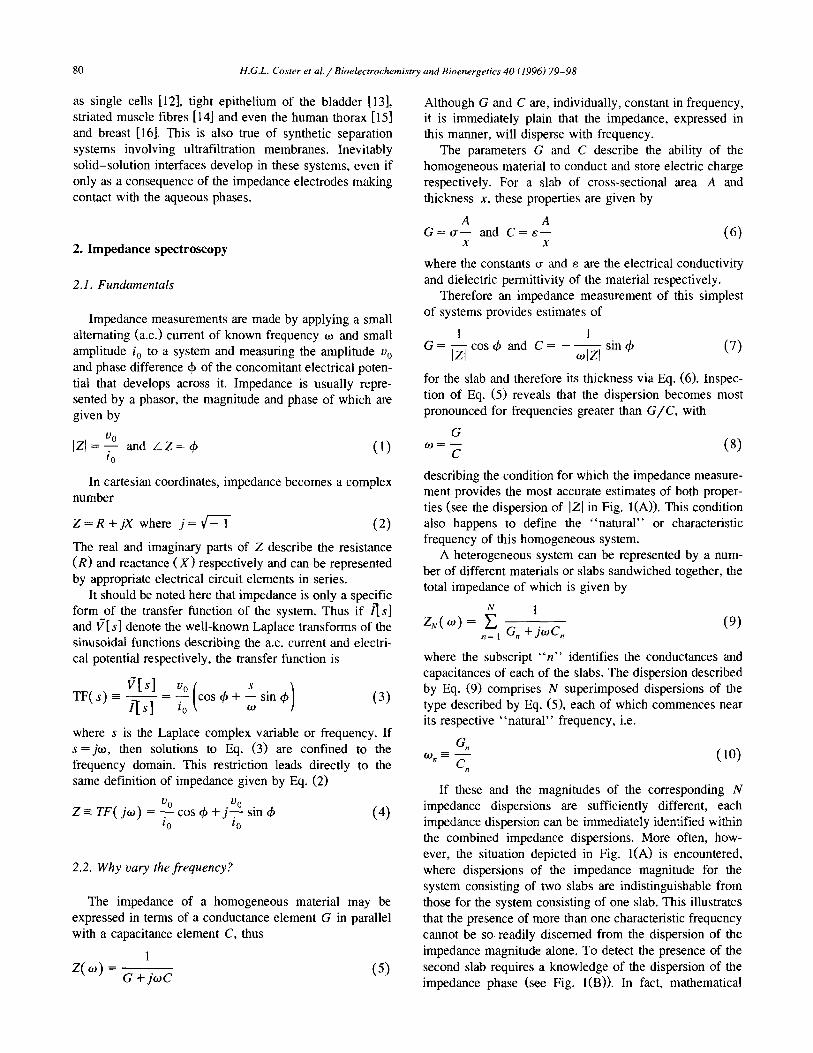
Even when the bulk solution adjacent to a surface (such as a membrane) is stirred, there is a region of static fluid immediately adjacent to the surface where thermal convec- tion or density gradients do not cause any significant mixing of the solution [34]. In most circumstances, unstirred layers are notorious for hindering measurements of membrane performance parameters. Unstirred layers can also give rise to strong dispersions in the impedance. As an example, we consider the role of unstirred layers when the transport numbers (fraction of total current carried by an ion species) for the ions in the bulk solution are different from those for the ions in the membrane separating two electrolyte solutions.

When electric currents flow through such an electrolyte-membrane-electrolyte system, the transport number differences give rise to concentration gradients in the unstirred layers (see Fig. 6(A)). When these gradients are perturbed by a very low-frequency electric field, the ions

86 H.G.L. Caster et al./ Bioelectrochemistry and Bioenergetics 40 (1996) 79-98

1 .o L r

ij .,()L l l

1 / / / I

1 10 100 1000

Hertz Fig. 6. (A) Illustration of how ionic concentrations can change in the unstirred layers next to the membrane-solution boundaries during the flow of electric current through a membrane in which the transport numbers of anions and cations in the membrane and solution are unequal. The relative fraction of the total current (i.e. transport number T) carried by each ionic species is indicated in the diagram by the width of the appropriate arrows. The arrows show the direction of the ionic flow. These differences in the transport numbers in the membrane and solution lead to an accumulation of both cations and anions on one side of the membrane and a depletion of the ions on the other side. The accumulation and depletion effects, and their effect on the impedance, are most pronounced at very low frequencies, but vanish at very high frequencies because there is then insufficient time during each half cycle of the a.c. current to modulate significantly the concentration profiles. (B) Examples of two distinct types of low-frequency dispersion characteristics of capacitance (open and filled circles) arising from differences in the transport number in a cell of Churn corallina. These very different types of dispersion in capacitance have identical dispersions in conductance (error bars smaller than the points drawn). The full lines are the theoretical dispersion for the ultrastructural model [35] fitted to the data (shown with error bars). These data indicated with error bars are the average of 16 spectra (and include the two very different spectra represented by the open and tilled circles).

diffuse slowly across the membrane, inducing a phase shift which can give rise to a “pseudo’‘-capacitance [36,37]. This capacitance, which disperses with frequency, is usually orders of magnitude larger than dielectric geometrical capacitances of the system. At higher frequencies, this diffusion polarization capacitance vanishes because the ion concentration gradients which build up in each half cycle of the a.c. current become negligible when the period of the a.c. signal is very short. In this respect, the dispersion is characteristic of an ‘x-type dispersion. Sometimes, elec- trophoretic effects [38] (i.e. a coupling of water flow to ionic fluxes) in the membrane and the unstirred layers give rise to a phase shift in the opposite direction, and this is manifested as negative capacitances or “pseudo”-induc- tance [39,40]. Such dispersions are distinctly different from the more usual ci type.

Examples of the two characteristic capacitance dispersions for the same plant membrane are shown in Fig. 6(B). Interestingly, the corresponding conductance dispersions for these two extreme examples are indistinguishable, indicating that the “capacitive” and “inductive” dispersions arise substantially from phase shifts induced by interference between impedance measurements and ionic diffusion currents established by polarization between the juxta- posed unstirred layers of the membrane. That these dispersions move to lower frequencies whenever the membrane conductance decreases [35] (not shown), demonstrates that ionic diffusion through the membrane, and hence the transport property differences between the ionic species therein, directly influences the polarization between the layers. Although these dispersions can be characteristically “capacitive” or “inductive”, at other times, the dispersion can fluctuate between these states as a function of frequency [35]. If sufficient individual impedance spectra are obtained over a longer time period, the averaged impedance dispersion spectrum (see theoretical curve in Fig. 6) is reminiscent of an a dispersion, even at low frequencies. The large experimental errors (e.g. see Fig. 6(B)) that arise as a consequence of this statistical averag- ing, however, identify the presence of transport number polarization effects in unstirred layers. At higher frequencies, these errors diminish with respect to the unstirred layer impedances, revealing characteristic CX- and B-type dispersions [35].

4.4. Bimolecular lipid membranes

It was found that, in an aqueous environment, lipids spontaneously assemble into various aggregates, including a bimolecular membrane structure. Initial measurements of the impedance of lipid membranes provided the first good estimates of the membrane thickness [6], from which it was confirmed that the membrane simply consisted of two molecular layers of lipid, from whence came the name bimolecular lipid membrane or BLM.

H.G.L. Caster et al./Bioelectrochemistry and Bioenergetics 40 (1996) 79-98 87

These early pioneering studies were restricted to measurements of the total impedance of the BLM- electrolyte-electrode system using bridge techniques. Later, studies [32] were based on accurate two-terminal impedance measurements of the BLM-electrolyte-electrode system as well as the electrolyte-electrode system alone (i.e. without the BLM), from which the impedance of the BLM was obtained by subtraction of the complex

components. The dispersions of the BLM capacitance and

conductance at low frequency provided the first insights into the substructure of the bilayer lipid membrane.

Precise data for the BLM itself, as distinct from that of the membrane and the metal electrodes together, required a four-terminal impedance measuring system [33], which was capable of measuring the impedance and phase very accurately, especially at ultralow frequencies. Earlier ver-

A

6.8 -

E

g 6.6 -

s 5 $ 6.4 -

4

6.2 -

l ImMKCI 0 IOmMKCI

. 1OOmM KCI

B

IO3 IO2 IO3 IO2 IO” 1 10’ IO2 10’ 10’ IO” 1 10’ IO2 10’ 10’ FREQUENCY HERTZ FREQUENCY HERTZ

IO’ IO’ l ImMKCI l ImMKCI 0 IOmM KC, 0 IOmM KC,

10’ 10’ . iCOmt.4 KCI . iCOmt.4 KCI

1 1

IO” IO”

1 o-2 1 o-2

lo-’ lo-’

C

C mFlm2

&,

IO” IO2 10-l 1 10’ lo2 IO3 10’

FREQUENCY HERTZ 1 nm

.i

60-30

. H2 \./ \./‘\./

\/\.A../

25.4

2.13

Fig. 7. The equivalent parallel capacitance (A) and conductance (B) of representative egg phosphatidylcholine bilayer-electrolyte systems formed from n-hexadecane solutions of the lipid (from Ref. [42]). The error bars (generally too small to be visible) give the standard error of three to five frequency scans on a single bilayer. (C) A schematic diagram of an egg phosphatidylcholine molecule showing the putative location of each distinct dielectric region determined from a Maxwell-Wagner model for the bilayer fitted to the data. The range of dielectric constant of each distinct layer so estimated is shown in the accompanying table for the case of a BLM in I mM KCl. The data are representative, in each case, of an average of ten phosphatidylcholine bilayers. The polar head of the phosphatidylcholine molecule is shown here at approximately 45” to the bilayer normal; however, other orientations are equally likely. The dielectric constant E,, capacitance C and thickness d of any region are related by C = .s,e,,/d, where E,, is the pennittivity of free space. H 1 and H2 refer to the hydrophobic regions, Al and A2 to the acetyl regions and Pl -P3 to the polar head regions. It must be stressed, however, that these dielectric regions need not correspond to specific regions of the phosphatidylcholine molecules, but, because of thermal motions, will represent both time and spatial average values over different parts of the phosphatidylcholine molecules.

88 H.G.L. Caster et al./Bioelectrochemistty and Bioenergetics 40 (1996) 79-98

sions (1974) of a computer-based instrument ( 10e2 Hz < o < lo* Hz) revealed the electrical and geometrical properties of the hydrophobic and hydrophilic structures of the BLM [7]. Improved versions (after 1983), capable of 0.01” accuracy at low frequencies, were able to resolve a further four layers within the hydrophilic regions [41], achieving resolutions of 0.1 nm over the range IO-* Hz < w < IO4 Hz (see Fig. 7).

The effects of external electrolyte [43], local anaesthet- its [44], growth hormones [45] and cholesterol [42] on BLMs have been characterized in this manner. Further- more, important advances in the understanding of the ways in which cholesterol [46] and temperature 1471 modulate the interactions between anaesthetics and BLMs have been made.

4.5. Interfacial polarization in cell suspensions

Although so far we have chosen to describe interfacial polarization impedance dispersions in terms of a system with planar geometry, the earliest examples were observed in a suspension of spherical cells. Models for this system were first developed by Maxwell [48] for the d.c. case and Wagner [49] for the a.c. case. The results are illustrated in Fig. 8, where the flow of current around a spherical cell is shown when an a.c. electric field is applied to the suspension. For low frequencies, the membrane effectively insu- lates the cytoplasm and current can only flow around the cell (see Fig. 8(A)). As the frequency increases and the membrane becomes more conducting, the current flow begins to depend on the ratio of the complex conductivity of the cytoplasm to that of the bulk solution, which is approximately equal to that of the conductivities alone at moderate frequencies (cf. Eq. (18)). For higher frequencies and hence higher ratios of the complex conductivities, interfacial polarization effects at the interfaces between the electrolyte and the membrane, as well as between the membrane and the cytoplasm, give rise to flow across the membrane into the cytoplasm (see Fig. 8(B)). The flow into the cytoplasm increases as this ratio increases further with increasing frequency (see Fig. 8(C)). It should be noted that, at sufficiently high frequencies, the ratio of the complex conductivities approaches that of the permittivity of the cytoplasm to that of the bulk solution. Since both are aqueous phases, this limiting ratio is approximately unity.

Further modelling by Fricke [50] led to the equivalent circuit for the suspension, shown in Fig. 8(D), the impedance of which is

1 -1

R, + l/(.bC,,,) 1 (31)

and contains contributions from the bulk solution (R,), the cytoplasm CR,) and the membrane (C,). It is clear from Fig. 8(A)Fig. 8(B)Fig. 8(C) that the presence of cells in the

C

II’

0

0 R. R. C.

E -Xohms

Fig. 8. Interfacial polarization in cell suspensions. Lines of current flow around a cell placed in a uniform a.c. field arc shown for increasing frequency ((A). (B) and (C)). (D) An equivalent circuit for a red blood cell suspension. R, represents the resistance of the electrolyte, R, the resistance of the cell cytoplasm and C, the capacitance of the cell membranes. The total impedance of the circuit is given by Eq. (31). (E) A complex impedance plane representation, R vs. - X, of cell suspension impedance data from Ref. (121.

suspension impedes the flow of current more strongly at low frequencies than at high frequencies. This is also described by Eq. (31), in which the impedance decreases from a value of R, at low frequencies to a value corresponding to R, in parallel with R, at high frequencies. Furthermore, Eq. (31) can be represented by a semicircle in the complex impedance plane (see Fig. 8(E)) from which these low- and high-frequency limits (denoted by R, and R, respectively) can be readily identified. Contri- butions of the membrane capacitance C, can be determined from the radius of the semicircular locus. Using appropriate impedance models developed especially for red blood cell suspensions [51,52], and assuming a dielectric constant for the membrane of approximately three, Fricke and Morse [4] made the first estimate of the thickness of a cell membrane in 1925. Their value of 3.3 nm indicated, for the first time, that the membrane thickness was of the order of molecular dimensions and was remark- ably accurate. 6

6 Modem estimates based on electron microscopy and X-ray crystal- lography give a value of 2.2 nm for the thickness of the central hydrophobic region of the membrane and 6 nm for the total thickness (e.g. [SD.

H.G.L. Caster et al./ Bioelectrochmistry and Bioenergetics 40 (1996) 79-98

By 193 1, Fricke had also shown that red blood cells from human, calf, dog, rabbit, chicken and turtle had the same membrane capacitance of 80 mF m-* and that this capacitance did not depend on the electrical properties of the suspending solution or the measuring frequency [53]. Subsequently, similar experiments on suspensions of spherical eggs of Arbaciu [54], Asterias [55] and frog [56] indicated that they had a membrane similar to red blood cells, as did single marine eggs [57]. This was also confirmed for cells of Valonia and Nitella [58] from the plant kingdom, and even for chloroplasts obtained from cells of Charu corallina [59].

Early impedance measurements of cell suspensions were technologically limited to mainly characterizations of the bulk electrical properties of the suspension and of the cell membrane and cytoplasm. These measurements established that the membrane had the properties of a parallel plate capacitor, but could not establish clearly to what extent the membrane was impermeable to ions. For that, other elec- trophysiological techniques were developed [58].

For the two decades after the Second World War, the emphasis of investigations of the electrical properties of cell membranes shifted from the frequency domain (impedance spectroscopy) into the time domain (voltage clamp), towards characterizing the voltage-dependent and time-dependent gating properties of the individual ionic permeation pathways [60]. Further improvements to early impedance models of cell suspensions [6 1,621 have been made to include the effects of charge 1631 on the cell membrane and diffusion through it [64]. Recent work by Gheorghiu [65] has also shown that impedance measurements of cell suspensions at low frequency can determine the membrane potential of the cells non-invasively.

4.6. Ultralow-frequency impedance dispersions in cell membranes

By 1964, impedance spectroscopy had established that lipid only forms an insulating matrix [6] for the proteins in biological membranes. Therefore the membrane proteins must form the ionic permeation pathways that confer the properties of selectivity and voltage gating to the cell membrane. Until pure transport proteins could be isolated and inserted into artificial lipid membranes, impedance studies for elucidating protein structure and function were confined to studies on the whole cell membrane.

Direct measurements using intracellular electrodes revealed strong dispersions in the impedance of the plasma membrane of cells [40,66-681. The observed impedance dispersion, as well as many of the other electrical characteristics [20,69-721 of these cell membranes, were similar to those of a membrane in which one half contains fixed positive charges whilst the other half contains fixed negative charges: the so-called double fixed charge membrane (DFCM). Additional evidence indicating that biological membranes have an overall charge structure which resem-

?$j 1

\

8 0.1 i-i 5 3 0.01

5 0 5 0.001

g 0.0001

0.1 10 100 1000 10000

Frequency Hz

IOOmV

EJz+\

5 0.01 k

t. , , , , , 0.1 1 10 100 1000 10000

Frequency /Hz

Fig. 9. Dispersions of the double fixed charge membrane (DFCM) conductance and capacitance with frequency as a function of the depletion layer potential difference (V,) (from Ref. [SO]). The dispersions are similar to those of a two-element Maxwell-Wagner system, but the elements required for the latter may not be identified with the separate regions of the DFCM. The capacitance at low frequencies arises from an enhanced capacity of these membranes to store electric charge. This low-frequency capacitance is dependent on V,. unlike that at high frequency which depends only on the dielectric and geometrical properties of the membrane.

bles a DFCM arose from impedance studies of the alkaline and acid regions which form at the surface of a single cell of Char-u [73]. These regions were strongly correlated with the observed spatial distributions of membrane conductance [74,75], low-frequency capacitance [76] and proton ATP synthase surface density [77], in a manner consistent with pH regulating the degree of ionization of fixed charges in a DFCM.

Derivations of the DFCM impedance commenced from considerations of the membrane capacitance [78]. How- ever, those based on solutions of the Nemst-Planck-Pois- son equations (Eq. (21) and Eq. (22)) showed that the capacitance and conductance dispersed with frequency [79] in a frequency range characteristic of an a-type dispersion. The dependences of the capacitance and conductance dispersions on the internal d.c. electrical potential (see Fig. 9) were also consistent with this classification. Only at high frequencies did these dependences diminish, indicating that the capacitance and conductance at these frequencies derive from the bulk electrical properties of the DFCM [66,81] (cf. Eq. (27)). The dispersion at these higher frequencies can therefore be characterized as B type. More

90 H.G.L. Caster et al. / Bioelectrochemistry and Bioenergetics 40 (1996) 79-98

recent analyses of the DFCM impedance have revealed that the overall dispersion can be represented by two characteristic frequency constants (E!q. (lo)), although such constants do not derive from layers (i.e. interfacial polarization effects) within the membrane [82].

4.7. Impedance dispersions arising from cell ultrastructure

Once the impedance of the cell membrane had been characterized, it was possible to identify other contributions to the measured impedance dispersions of cells. These contributions essentially arise from interfacial polarization effects between ultrastructural regions within the cell. Impedance spectroscopy studies have been able to characterize cell ultrastructure electrically, such as the static cytoplasm [83], charasomes [84] and the plasma membrane coat [35]. Based on these ultrastructural characterizations and those of the electrode-electrolyte interface, it has been possible to extend these studies to other functionally important organelles in plant cells, such as plasmodesmata [85], which are pore-like structures form- ing cytoplasmic connections between cells [86] for the regulation of the growth and development of the whole plant.

For the plant cell systems, the knowledge gained from impedance studies of individual molecular structures in isolation (such as the plasmalemma or tonoplast membranes) has formed the framework for impedance studies of the macroscopic cellular system in which these molecular structures are embedded.

4.8. Synthetic membranes

The following summarizes the progress which has been made in fundamental impedance studies of a variety of synthetic membrane systems.

4.8.1. Ultrafiltration membranes A knowledge of the skin layer morphology of synthetic

polymeric membranes, used in reverse osmosis and ultrafiltration, can help to elucidate their separation mechanism, since the pore structure and distribution determine the intrinsic permeation properties. Fig. 10 shows a schematic representation of an ultrafiltration membrane depicting the skin layer supported by the more open sublayer. The equivalent electrical circuit of the membrane-electrolyte system is shown. The elements of this equivalent circuit can be determined, non-invasively, from four-terminal impedance measurements in the frequency range 103-lo4 Hz using electrodes placed in the external electrolytes [87]. At these frequencies, contributions to the total impedance from unstirred layers and fixed charges (see Fig. 6 and Fig. 9) will be negligible and need not be taken into account. From a knowledge of the dielectric constant of water and that of the membrane polymer, the porosity of the membrane may be estimated from the value for the capacitance

skin layer sub layer

-7 \ / pores current flow

3 \ c I T electrolyte electrolyte

SW--

Gskin Gsub Fig. 10. An equivalent circuit of an ultrafiltration membrane-electrolyte system. The skin and sublayers of the membrane are each represented by the parallel combination of a conductance (G) and capacitance (C) element. The slices of electrolyte between each membrane surface and the plane containing the adjacent voltage electrode are represented by the conductance elements G&t and Gi,,, (from Ref. [87]).

of the skin layer (CSkin) determined by impedance spectroscopy.

4.8.2. Supported liquid membranes The principles outlined above have also been applied to

supported liquid membranes (SLMs). In these membranes, the polymer membrane matrix is filled with organic liquids in which the solute(s) of interest in the feed stream (which is often an aqueous solution) is more soluble than in the membrane-supported liquid. In this way, highly selective membrane filtration systems can be constructed, particularly for the removal of organic compounds from aqueous solutions. One problem with SLMs is that the feed solution gradually displaces the liquid supported by the polymeric membrane, i.e. membrane liquid is lost to the adjacent aqueous solution [88]. Using impedance spectroscopy, it is possible to monitor the dynamics of this process. This displacement of the membrane liquid is observed as an increase in the total capacitance when membrane liquid of low dielectric constant is displaced by an aqueous solution of high dielectric constant.

4.8.3. Electrically conducting synthetic membranes Conducting synthetic membranes may be used to advan-

tage in electrically driven separation processes, because electric fields can be generated via direct electrical contacts with the membrane or between the membrane and the aqueous solution. By varying the field strength and direction of the electric field in/or through the conducting membrane, the surface charge densities and concentration polarization of the solute-membrane interfaces and electric double layer (within which the adsorption of solutes

H.G.L. Caster et al. /Bioelecfrochemistry and Bioenergetics 40 (1996) 79-98 91

I current flow

double layer \

electrolvte

2 J! metal

Fig. 11. Schematic cross-section of a conducting (metal-coated) membrane. The electrical current used for the impedance measurements enters the membrane via direct electrical contacts with the membrane and passes along its metal surface. The current so injected also couples to the solution via the ionic double layer at the interface between the metal coating and tire solution.

presumably leads to fouling) can perhaps be modulated, thereby controlling both the separation characteristics and the fouling processes. Impedance spectroscopy immediately suggests itself as a method for monitoring the effects of the field on these membrane processes.

For instance, one crucial parameter in using conducting membranes is the intrinsic conductivity of the membrane. The monitoring of this during separation processes can be achieved using measurements of the longitudinal impedance (in the plane of the membrane). Impedance measurements of the membrane can be made with electrodes attached directly to the metal surface (see Fig. 11). At low frequencies, the current used for the impedance measurements will pass mainly through the metal because the double layer impedance, which is very large at these frequencies, will insulate the metal from the electrolyte, even within the pores. Thus impedance measurements at these frequencies can be used to determine the intrinsic conductivity.

As the double layer impedance becomes smaller with increasing frequency, its insulating properties diminish, and the impedance measurements increasingly reflect the properties of the electrolyte, double layer and the pores [89]. Therefore longitudinal impedance measurements at these frequencies can also monitor other important membrane processes.

4.8.4. Bipolar membranes In bipolar membranes, the inner part of the membrane

contains fixed charges of one sign, whilst the outer part contains fixed charges of the opposite sign. They are the synthetic equivalent of the DFCM already discussed in the context of cell membranes earlier. Bipolar membranes are used in the recovery of recyclable products from industrial waste. They are used for the regeneration of acids and

alkalis from salts in waste solutions and other industrial chemical processes [90-921.

Impedance studies of bipolar membranes [81,93] reveal similar capacitance dispersions (see Fig. 9) to those reported for biological membranes [66]. Further theoretical studies [SO] and impedance characterizations using a new presentation of spectra [82] may provide insights into methods to optimize separation processes performed by synthetic bipolar membranes.

5. Advanced interpretation techniques

As we have seen, impedance data can be presented in a variety of ways. A common notion in these presentations is the concept of “time constants” or their reciprocals (“frequency constants”). This concept is particularly appropriate for a system of planar layers in which interfacial polarization effects lead to a dispersion of the impedance with frequency. However, it also applies to systems which exhibit ionic diffusion polarization [82] as well as active transport processes. The notions of “time” and “frequency” arise from the same set of differential equations which describe the electrical response of the system. The Laplace transforms of these response functions lead to an expression of the system’s transfer function [94] which, for all the systems described so far, has the general form

TF(s)= 2 ‘n n=l JfW,

(32)

where o, are the frequency constants and rn are the residues which can be determined [95] directly from the integral of Eq. (32), thus

1 r E- n 2rj #

TF( s)ds (33) S-*-W”

As described for Eq. (3) and Eq. (4), the restriction s = jw leads directly to an expression for the impedance of N slabs sandwiched together (i.e. Eq. (9)), where the frequency constants are given by Eq. (10) and the “residues” are given by

1 rn = -

cl2 (34)

However, Eq. (9) is a general form of the impedance of many systems in which the C, values need not necessarily derive from geometrical capacitances and, in some special circumstances, may be negative or even complex.

As an example of the more general form of the transfer function, we present a plot (Fig. 12) of its magnitude for a system with two time constants as a function of the Laplace variable ‘Is”. However, this variable has real (a> and imaginary (w) components, and therefore the transfer function can be presented as a three-dimensional plot in the variables u and o.

92 H.G.L. Caster et (II./ Bioelectrochemistry and Bioenergetics 40 (1996) 79-98

When s is real and negative, the transfer function has discontinuities at

s= -id,,- 02 (35) These points of discontinuity are discernible as peaks in the three-dimensional surface in Fig. 12. The positions of the peaks correspond to the magnitude of the frequency constants of the system.

The integral of the transfer function along the negative u axis is

1 Ip = -

/ -bF( s)ds 23-j s=o (36)

which is shown below the three-dimensional representation of the transfer function in Fig. 12. The steps in the integral align with the transfer function peaks and the size of the steps gives the residues (Eq. (33)). Thus the transfer function (Eq. (32)) and the integral (Eq. (36)) reveal all the important electrical parameters of the system.

TW t TF(s=-cr)

\

Transfer Function

Fig. 12. Three-dimensional representation of the magnitude of the transfer function for a two-layer system (cf. Eq. (32) for N = 2). For s = jw, the transfer function becomes the impedance, which can be seen to disperse with frequency in the same manner as depicted in Fig. l(A). For s < 0, the transfer function resembles a spectrum in which two peaks identify the frequency constants or “natural” frequencies, W, and 02. of the system (Eq. (10)). Shown beneath the transfer function is the integral of the transfer function along the negative frequency axis (Eq. (36)). The steps in the integral identify the parameters r, and rz in the transfer function.

Fig. 13. Transfer function spectra for bimolecular membranes of lecithin (A) showing the effects on the peaks (frequency constants) of the addition of cholesterol (B) and cholesterol plus cyclosporin-A (Cl (see Fig. 7(C) for a schematic diagram of the lecithin molecule which identifies the regions referred to by labels on the spectra shown).

Algorithms have been developed for fitting Eq. (9) to impedance data [17]; thus the transfer function (Eq. (32)) can be readily obtained and displayed for most systems. Fig. 13 illustrates this utility for the transfer function “spectra” obtained from impedance measurements [96] of BLMs made from phosphatidylcholine (lecithin). The positions of the peaks in the spectra identify the frequency constants for the membrane system. These constants can be identified with the corresponding substructural layers of the lecithin molecule (cf. Fig. 13(A) and Fig. 7(C)).

The effect of the addition of cholesterol in the BLM is shown in the spectrum in Fig. 13(B). This shows that the peaks corresponding to regions containing the acetyl (oxygen) moieties and, to a lesser extent, those corresponding to the glycerol bridge region are shifted to higher frequencies. In contrast, the peak corresponding to the hydrocarbon region is shifted to lower frequencies. These shifts identify the substructural regions in which the cholesterol and lecithin molecules interact within the BLM. The shift in the hydrocarbon peak is related to changes in thickness of the hydrocarbon region when cholesterol is added to lecithin membranes. The shift in the acetyl peak

H.G.L. Crater et al./ Bioelectrochemistry and Bioencrgetics 40 (1996) 79-98 93

OCCURS because the OH group on the cholesterol aligns

with the acetyl groups on the lecithin molecules.

Fig. 13(C) shows a spectrum for a lecithin-cholesterol BLM to which cyclosporin-A (an immunosuppressant drug used in transplant therapy) has been added. The shifts in the peaks, in this instance, indicate a profound effect of cyclosporin-A on the polar head region, but only a very small effect on the hydrocarbon region of lecithin- cholesterol BLMs.

The impedance dispersions for this system [97] have shed light on the location and orientation of cyclosporin-A. The alternative presentation, using the transfer function “spectra”, facilitates a direct physical interpretation of these effects, from whence a better understanding can be obtained of the physiological role of cyclosporin-A as an immunosuppressant drug in transplant therapy.

6. Ultralow-frequency impedance spectrometer

The a.c. impedance can, in principle, be measured using a bridge. However, determining the null point becomes difficult and tedious for the very low frequencies (typically 0.01 - 100 Hz) necessary for characterizing many biological and synthetic systems. These very low-frequency impedance measurements only became feasible when com- puters became sufficiently miniaturized and affordable and digital technologies were developed for precision computer-controlled data acquisition of analogue signals. This provided the basis for the development of the first computer-controlled ultralow-frequency impedance spectrometer [331. While some commercial instruments are now available, they generally do not offer sufficient resolution simultaneously in phase and magnitude over the entire frequency and impedance ranges of interest for the systems reported here.

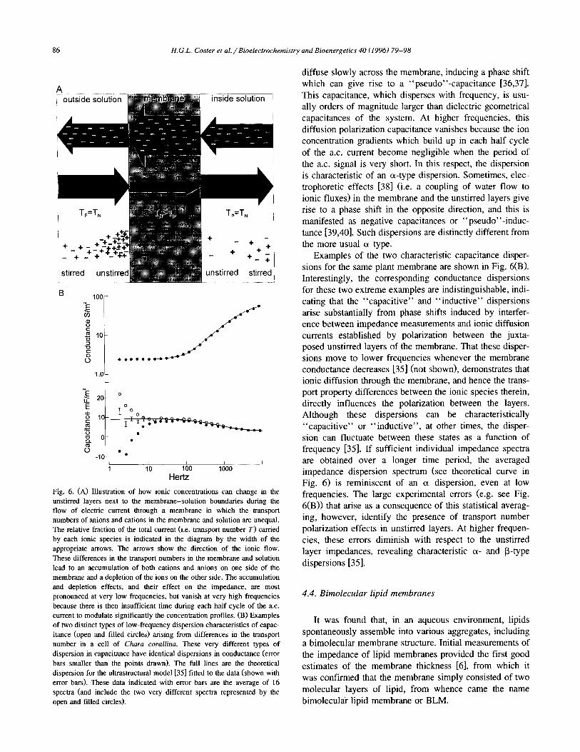
We have now constructed a digital impedance spectrometer capable of a phase resolution to 0.001” and impedance magnitude resolution to 0.002% over the frequency range O.Ol- 100000 Hz for impedances in the range lo-lo9 fl (see Fig. 14).

6.1. Principles of operation

The accurate measurement of the impedance requires the simultaneous measurement of the magnitude of the sinusoidal current and voltage and the phase shift between them. In the present technique, both the magnitude and phase shift are measured by sampling the current and voltage at precisely phase-locked intervals during a cycle of the a.c. signal. The magnitude and phase shift can then be very precisely obtained by fitting sine functions (of predetermined frequency) to these digital data.

The basic functional units of the ultralow-frequency impedance spectrometer are a signal generator board and two data acquisition boards that are interconnected via a

(0.02%) t

: 1000.7 +

I .

1 10 100 1000 10000 100000 Frequency/Hz

0.01

I

-0.01 I .-.-____

i l-0 160 IciOO 10000 100000 Frequency /Hz

Fig. 14. Typical performance characteristics of the new impedance spec trometer. Impedance measurements of a 1000.60 ( !L 0.02) R resistor are shown for frequencies ranging from I to IO5 Hz. The signal amplitude for these measurements was set to 20 mV. a level which was suitably small for most membrane characterizations. The standard errors for the magnitude and phase are approximately 0.002% and 0.001” for all individual frequencies, except at 50 Hz (as expected; the line frequency in Australia) and frequencies approaching 10’ Hz. The magnitude and phase are independent of frequency to within +O.C02% for the magnitude and +O.OOl” for the phase at frequencies below lo4 Hz. For frequencies greater than IO4 Hz, the margins are well within those determined for the previous version of the spectrometer (i.e. & 0.02% for the magnitude and 50.01” for the phase). The performance characteristics were typical of resistors with higher values once the effects of amplifier “stray” capacitances, and the frequency dependence of these, were accounted for (not shown). Even better characteristics were obtained for amplitudes greater than 20 mV and amplifiers with smaller gains (not shown).

mother board. The spectrometer interfaces to a computer through a 32-bit bidirectional parallel interface. A block diagram of the main aspects of the ultralow-frequency impedance spectrometer is given in Fig. 15.

6.2. Signal generation

A very pure sinusoidal signal is synthesized digitally on the signal generator board. To achieve this a sine function table is loaded into a 65k X 16-bit random access memory (RAM) located on the board. By clocking this RAM, the table entries are latched sequentially onto a 16-bit digital- to-analogue converter (DAC), producing a raw ax. analogue signal. Filters remove the digital glitches from the signal and generate a smooth low-distorted sinusoidal signal, the amplitude and offset of which can also be controlled by the computer. The a.c. amplitude is maintained at less than 20 mV in order to avoid distortion of the a.c.

94 H.G.L. Caster et al. / Bioelectrochemistry and Bioenergetics 40 (1996) 79-98

From s-.

,’ *. . computer .._a’

MU+ FWJI

,./“.., ..: \

: .,., / %

DAC Filter

I 77-l A clock

I L I [+XZinal cOnfigUMi0n/ __. - - t I

‘. ‘.._.,

7. ‘....._,I “..pC offset ‘....._

Yzl DAC

’ ? t ADC I

To computer

control latches I

From computer

Fig. 15. Schematic diagram of the computer-controlled ultralow-frequency impedance spectrometer. Depicted are the random access memory (RAM), the digital-to-analogue converter (DAC) and the filter which together generate the undistorted sinusoidal (a.c.) analogue signal which is applied to the series combination of the standard impedance and the unknown system. The a.c. signals which develop across the standard and the system are amplified with high-input impedance (10” fI) differential amplifiers (A = loo), measured with separate analogue-to-digital converters (ADCs) and stored in the appropriate RAMS. The signal generation and data acquisition are controlled by a single clock, the rate of which is pro- grammed by the control latches via the computer. Separate computer-controlled DACs offset d.c. signals that could be otherwise present at the outputs of each amplifier.

signal by non-linear characteristics within the system. The clock derives from programmable digital frequency di- viders driven by an extremely stable (drift, less than 3 ppm) crystal oscillator. This clock also provides the timing for the sampling of the current and voltage.

6.3. Four-terminal configuration

The four-terminal configuration eliminates the effects of the (frequency-dependent) impedances arising from electrode-solution interfaces (see Section 4.2).

The signal is applied to the series combination of the standard impedance and the unknown impedance. The standard impedance consists of accurately known circuit components (resistors and capacitors) comprising a Maxwell-Wagner network of one, two or three elements.

These components are chosen such that the impedance dispersion of the standard is similar to that of the unknown system. This arrangement ensures that the potentials developed across the standard and unknown are very similar, and this allows the two high-input impedance amplifiers to operate with the same maximum gain settings to optimize the signal-to-noise ratio (SNR) over the whole frequency range.

6.4. Data acquisition

The sampling of the a.c. electrical potentials that develop across the standard impedance and the system is performed with separate data acquisition boards. Each board contains both fast (12-bit, 10 MHz) and high-resolution (16-bit, 500 kHz) analogue-to-digital converters (AD&) that write into a 65k X 16-bit RAM. The sampling of the two signals (voltage and current) is phase locked as the sampling triggers are derived from the same clock as used to generate the sinusoidal signal applied to the unknown impedance. This enables the independent and accurate determination of the phase difference between these responses.

Effectively, 65k samples of each a.c. electrical potential cycle are obtained, temporarily stored in the “on board” RAMS and then transferred to the computer memory where an optimized least-squares sinusoidal fitting routine (writ- ten in machine code to speed up the operations) determines the magnitude, phase, offset and SNR for each data set.

The SNR is a quantitative estimate of the sinusoidal quality which further indicates the accuracy to which the magnitude and phase have been determined. Data acquisition is repeated if the SNRs are not sufficiently large. The software appropriately compensates for d.c. offsets and/or adjusts the amplitude and filter in order to maximize the SNRs.

6.5. Spectrometer calibration

The measured magnitudes and phases of the a.c. responses need to be corrected for frequency-dependent anomalies in the gains of the amplifiers and/or within the instrument in general. These gain corrections are experimentally determined in a calibration procedure using precision resistors and capacitors for the “unknown”. The stray capacitances of the amplifiers are also measured during this procedure. The instrument characteristics for each frequency used are stored in the parameter file to correct any future measurements.

6.6. Software control

The computer software initiates signal generation at various frequencies from a file containing parameters for programming the clocks, amplitudes, offsets and filters on the signal generator board. The parameter file also contains

H.G.L. Caster et al./ Bioelectrochemistry and Bbenergetics 40 (1996) 79-98 95

the sampling rates for data acquisition at these frequencies, as well as the instrument characteristics for correcting the amplifier gains and stray capacitances. After acquisition, the software computes the magnitudes, phases and frequencies of the impedances as well as the SNRs and the d.c. levels. The results are stored in a separate data file.

6.7. Calculation of impedance

Once the magnitude and phase for the two signals (across the standard and unknown impedances) have been determined, the impedance magnitude and phase for the unknown are calculated using the known values of the components in the standard impedance and the stray capacitances present across each amplifier.

The software then repeats the operations for the next entry in the parameter file until all impedance measurements at the selected frequencies have been completed.

6.8. Special design features

68.1. Circuit boards The signal generator and the data acquisition boards

utilize four layers to achieve a high packing density of ADCs, DACs, RAMS, clocks, decoders and associated control circuitry and for providing ground planes to shield highly sensitive analogue components from external noise and digital interference. Further minimization of noise is achieved by powering these sensitive components with separate power supplies that are electrically isolated from the main power source and appropriately filtered.

The optical isolation of digital lines controlling analogue components on the signal generator board further minimizes the transmission of digital noise to the analogue output. This feature also renders this output floating, thereby eliminating a ground loop which is another likely source of noise.

These design features make it possible to achieve the full 16-bit resolution of the high-resolution (0.5 MHz) ADCs and, at the same time, provide the very short electrical connections necessary to achieve the 10 MHz sampling rates of the fast (12-bit) ADCs.

6.8.2. Cables All analogue connections between the signal generator,

amplifiers and data acquisition boards are via 50 fi cables. The correct termination of these cables ensures that distortion of the transmitted signals does not arise from reflec- tions. A.c. signals are transmitted differentially in order to further minimize ground loop noise. Line drivers capable of driving 50 fi and maintaining the 16-bit linearity specifications of the data acquisition system are used to drive the cables.

6.8.3. Amplijers The resolutions achieved with the signal generator and

data acquisition boards can be completely lost if the

amplifiers are not optimally designed for the four-terminal configuration which is so important in eliminating the contributions from electrode-solution interfaces. The four-terminal configuration requires that the amplifiers am- plify low-level differential signals (such as those which develop across the standard impedance and the system), while rejecting unwanted common-mode signals of the electrode-solution interfaces. Thus the common-mode re- jection (CMR) specification becomes a very important consideration in the amplifier design for this application [981.

Good CMR specifications are obtained when resistors integrated into the amplifier IC are accurately matched. However, at high frequencies, stray capacitances within the IC reduce this accuracy, resulting in a deterioration of CMR performance, and in the case of impedance measurements, erroneous dispersions with frequency. The best CMR performance is achieved when the common-mode signal is small and the differential signal is symmetrical about the IC ground. For this situation, the adverse effects of stray capacitances tend to cancel, resulting in a better CMR performance overall, as well as at high frequencies.

These optimal CMR conditions can be realized for each amplifier used in the four-terminal configuration if their power supplies are subregulated independently of the four-terminal circuitry, such that the common-mode signals, with respect to the respective amplifier grounds, are zero. Although analogue circuits are available for common-mode driven supplies [99], our design philosophy is for the software to determine the common-mode signals and drive the supplies. This provides a stable four-terminal front end which can accommodate a wide range of impedances (lo-lo9 a) and frequencies (lo-*-10’ Hz).

7. The future of impedance spectroscopy

The submolecular resolutions that can be achieved using impedance measurements of BLMs, for example, are ultimately limited by the resolutions available in the impedance magnitude and phase. A number of other av- enues for improving the SNR have recently been developed [lOO]. We are confident that the improvements now in hand will enable structural-functional impedance studies of proteins inserted in BLMs to be performed. The improvements in phase resolution will be of equal signifi- cance in synthetic membrane studies, where capacitance measurements of highly conducting systems can reveal membrane and double layer structures that are important to the membrane separation function. Novel methods [ 101,102] to obtain rapid (even real-time) evaluation of impedance may open new areas of application. We further foresee applications in studies of electrochemical processes occurring at interfaces and unstirred layers in such diverse systems as synthetic catalytic membranes and sensing electrodes. These fundamental studies will form the basis for

96 H.G.L. Cos~er et al./ Bioelectrochemistry and Binenergetics 40 (1996) 79-98

interpreting impedance data from cells and other biological tissues. Novel imaging tomography applications in both plants and animals may also emerge.

References

[I] R. HGber, Eine Methode, die elektrische Leitfahigkeit im Innem von Zellen zu messen. Arch. Ges. Physiol.. 133 (1910) 237-259.

[2] J. Bernstein, Uber den zeitlichen Verlauf der negativen Schwankung des Nervenstroms, Arch. Ges. Physiol., I (1868) 173-207.

[3] E. Overton, Ueber die allgemeinen osmotischen Eigenschaften der Zelle, ihre vermutlichen Ursachen und ihre Bedeutung fur die Physiologic, Vjschr. Naturf. Ges. Zurich, 44 (1899) 88- 113.

[4] H. Fricke and S. Morse, The electrical resistance and capacity of blood for frequencies between 800 Hz and 4.5 MHz, J. Gen. Physiol., 9 (1925) 153-167.

[5] J.D. Robertson, The molecular structure and contact relationships of cell membranes, Prog. Biophys., IO (1960) 343-418.

[6] T. Hanai, D.A. Haydon and J.L. Taylor, An investigation by electrical methods of lecithin-in-hydrocarbon films in aqueous solution, Proc. R. Sot. London, Ser. A, 281 (1964) 337-391.

[7] H.G.L. Coster and J.R. Smith, The molecular organisation of bimolecular lipid membranes. A study of the low frequency Maxwell-Wagner impedance dispersion, Biochim. Biophys. Acta. 373 (1974) 151-164.

[8] R.G. Ashcroft, H.G.L. Coster, D.R. Laver and J.R. Smith, The effects of cholesterol inclusion on the molecular organisation of bimolecular lipid membranes, B&him. Biophys. Acta, 730 (1983) 23 l-238.

[9] T.C. Chilcott, S. Frost-Shartzer, M.W. Iverson, D. Garvin, L.V. Kochian and W.J. Lucas, Potassium transport kinetics of KATl expressed in Xenopus oocytes: a proposed molecular structure and field effect mechanism for membrane transport, C.R. Acad. Sci., 318 (1995) 761-771.

[lo] J.R. MacDonald and J.R. Garber, Analysis of impedance and admittance data for solids and liquids, J. Electrochem. Sot.: Elec- trochem. Sci. Technol., 124 (7) (1977) 1022- 1030.

[11] J.B. Bates, J.C. Wang and Y.T. Chu, Impedance of metal-solid electrolyte interfaces, Solid State tonics, 18/l 9 (I 986) 1045- 1049.

[12] K.S. Cole, Membrane, Ions and Impulses, University of California Press, Berkeley, 1972.

[13] C. Clausen, S.A. Lewis and J.M. Diamond, Impedance analysis of a tight epithelium using a distributed resistance model, Biophys. J., 26 (1979) 291-318.

[14] G. Falk and P. Fatt, Linear electrical properties of striated muscle tibres observed with intracellular electrodes, Proc. R. Sot. London, Ser. B, 160 (1964) 69-123.

[15] R.P. Henderson and J.G. Webster, An impedance camera for spatial specific measurements of the thorax, IEEE Trans. Biomed. Eng., BME-25 (1978) 250-254.

[16] R. Skidmore, J.M. Evans, D. Jenkins and P.N.T. Wells, A data collection system for gathering electrical impedance measurements from the human breast, Clin. Phys. Physiol. Meas., 8 (Suppl. A) (1987) 999102.

[17] E.C. Levy, Complex curve fitting, IEEE Trans. Automatic Control, 4 (1959) 37-43.

[I81 H.P. Schwan, Electrical properties of tissues and cell suspensions, in Advances in Biological and Medical Physics, Vol. 5, Academic Press, New York, 1957, pp. 147-209.

1191 W. Nemst, Die elektromototische Wirksamkeit der Ionen, Z. Phys. Chem., 4 (1889) 129-181.

[20] H.F.L. Coster, The double fixed charge membrane: solution-membrane ion partition effects and membrane potentials, Biophys. J., 13 (1973) 133-142.

[21] P. Debye, Polar Molecules, Chemical Catalog Co., New York, 1929.

[22] J.L. Oncley, The electric moments and the relaxation times of proteins measured from their influence upon the dielectric constants of solutions, in E.J. Cohn and J.T. Edsall (Eds.), Proteins, Amino Acids and Peptides, Reinhold, New York, 1943, pp. 543- 568.

[23] S. Takashima, Dielectric properties of proteins. I. Dielectric relaxation, in Physical Principles and Techniques of Protein Chemistry, Part A, Academic Press, New York, 1969, pp. 291-333.

[24] A.C.F. Coster, H.G.L. Coster, T.C. Chilcott, J.R. Smith and J. Wolfe, Ultra low frequency impedance of the gold-electrolyte interface, in preparation.

[25] J.B. Hasted, D.M. Ritson and C.H. Collie, Dielectric properties of aqueous ionic solutions, J. Chem. Phys., 16 (1948) 1.

[26] D.C. Grahame, The electrical double layer and the theory of electrocapillarity, Chem. Rev., 31 (1947) 44-501.

[27] R. de Levie, The influence of surface roughness of solid electrodes on electrochemical measurements, Electrochim. Acta, 10 (1965) 113-130.

[28] T.C. Halsey, Frequency dependence of the double layer impedance at a rough surface, Phys. Rev. A, 35 (19861 3512-3521.

[29] L. Nyikos and T. Pajkossy, Fractal dimension and fractional power frequency-dependent impedance of blocking electrodes, Elec- trochim. Acta, 30 (1985) 1533-1540.

[30] S.H. Liu and T. Kaplan, AC response of fractal interfaces, Solid State Ionics, 18 (1986) 65-71.

[31] W. Geertsma and J.E. Gols, Theoretical model of the impedance of a fractal metal-solution interface, Physica A, 158 (1989) 691-705.

[32] H.G.L. Coster and R. Simons, Anomalous dielectric dispersions in bimolecular lipid membranes, B&him. Biophys. Acta, 203 (1970) 17-27.

[33] D.J. Bell, H.G.L. Coster and J.R. Smith, A computer based, four terminal impedance measuring system for low frequencies, J. Phys. E, 8 (1974) 66-70.

[34] P.H. Barry and J.M. Diamond, Effects of unstirred layers on membrane phenomena, Physiol. Rev., 64 (3) (1984) 763-872.

[35] T.C. Cbilcott and H.G.L. Coster, AC impedance measurements on Chara corallina. III. Characterisation of the plasma membrane coat using a new presentation of impedance spectra, Aust. J. Plant Physiol., 21 (1994) 147-168.

[36] J.R. Segal, Electrical capacitance of ion-exchanger membranes, J. Theor. Biol., 14 (1967) 1 l-34.

[37] P.H. Barry, Transport number effects in the transverse tubular system and their implications for low frequency impedance measurement of capacitance of skeletal muscle fibres, J. Membr. Biol., 34 (1977) 243-292.

[38] J.R. Smith, Electrical characterisation of biological membranes in different environments, Ph.D. Thesis, University of New South Wales, Sydney, Australia, 1977.

[39] K.S. Cole and R.F. Baker, Longitudinal impedance of the squid giant axon, J. Gen. Physiol.. 24 (1941) 771-788.

1401 H.G.L. Coster and J.R. Smith, Low-frequency impedance of Chum corallina: simultaneous measurements of the separate plasmalemma and tonoplast capacitance and conductance, Aust. J. Plant Physiol., 4 (1977) 667-674.

[41] D.R. Laver, J.R. Smith and H.G.L. Coster, The thickness of the hydrophobic and polar regions of glycerol monooleate bilayers determined from the frequency-dependence of bilayer capacitance, Biochim. Biophys. Acta, 772 (1984) l-9.

[42] R.G. Ashcroft, H.G.L. Coster, D.R. Laver and J.R. Smith The effects of cholesterol inclusion on the molecular organisation of bimolecular lipid membranes, B&him. Biophys. Acta, 730 (1983) 23 l-238.

[43] J.R. Smith, H.G.L. Coster and D.R. Laver, The dependence of the conductance of phosphatidylcholine bilayers upon the concentra

H.G.L. Caster et d./ Bioelectmchemistry and Bioenergetics 40 (19961 79-98 97

tion and composition of the external electrolyte, Biochim. Biophys. Acta, 812 (1985) 181-192.

[44] R.G. Ashcroft, H.G.L. Coster and J.R. Smith, The molecular organisation of bimolecular lipid membranes. The effect of benzyl alcohol on the structure, B&him. Biophys. Acta, 469 (1977) 13-22.

1451 U. Zin~mermann, R.G. Ashcroft, H.G.L. Caster and J.R. Smith, The molecular organisation of bimolecular lipid membranes. The effect of KC1 on the location of indoleacetic acid in the membrane, Biochim. Biophys. Acta, 469 (1977) 23-32.

[46] H.G.L. Coster and D.R. Laver, The effect of benzyl alcohol and cholesterol on the acyl chain order and alkane solubility of bimolecular phosphatidylcholine membranes, Biochim. Biophys. Acta, 861 (1986) 406-412.

[47] H.G.L. Caster and D.R. Laver, The effect of temperature on lipid- n-alkane interactions in lipid bilayers, B&him. Biophys. Acta, 857 (1986) 9S- 104.

[48] J.C. Maxwell, Treatise on Electricity and Magnetism, Oxford Uni- versity Press, London, 1873.

[49] K.W. Wagner, Arch. Electrochem.. 2 (1914) 371. [XI] H. Fricke, The electric capacity of cell suspensions, Phys. Rev., 21

(1923) 708-709. [51] H. Fricke, A mathematical treatment of the electrical conductivity

of colloids and cell suspensions, J. Gen. Physiol., 6 (1924) 375-384. [52] H. Fricke, A mathematical treatment of the electrical conductivity

and capacity of dispersive systems. I. The electrical conductivity of a suspension of homogeneous spheroids, Phys. Rev., 24 (1924) 575-587.

[53] H. Fricke, The electrical conductivity and capacity of disperse systems, Physics, 1 (1931) lO6- 115.

[54] KS. Cole, Electric impedance of suspensions of Arhaciu eggs, J. Gen. Physiol., 12 (1928) 37-54.

[55] KS. Cole and R.H. Cole, Electric impedance of Asterias eggs, J. Gen. Physiol., 19 (1936) 609-623.

[56] K.S. Cole and R.M. Guttman, Electric impedance of the frog egg, J. Gen. Physiol., 25 (1942) 765-775.

[57] K.S. Cole and H.J. Curtis, Electric impedance of single marine eggs, J. Gen. Physiol., 21 (1938) 591-599.

[58] L.R. Blinks, The effects of current flow in large plant cells, Cold Spring Harbor Symp. Q. Biol., 4 (1936) 34-42.

[59] A.B. Hope, The electrical properties of plant membranes, Aust. J. Biol. Sci., 9 (1956) 53-66.

[60] A.L. Hodgkin, The ionic basis for nerve conduction, Science, 145 (1964) 1148-l 154.

[61] H. Danzer, Uber das verhalten biologischer Korper bei Hochfre- quenz, AM. Phys., 21 (1934) 783-790.

[62] H. Pauly and H.P. Schwan. Uber die Impedanz einer suspension von kugelfomrigen Teilchen mit einer Schale, 2. Naturforsch., Teil B, 14 (1959) 125-131.

[63] A. Garcia, R. Barchini and C. Grosse, The influence of diffusion on the permittivity of a suspension of spherical particles with insulating shells in an electrolyte, J. Phys. D, 18 (1985) 1891-1896.

[64] E. Gheorghiu, The dielectric behaviour of suspensions of spherical cells: a unitary approach, J. Phys. A, 27 (1994) 3883-3893.

[65] E. Gheorghiu, The resting potential in relation to the equivalent complex permittivity of a spherical cell suspension, Phys. Med. Biol., 38 (1993) 979-988.

[66] H.G.L. Coster and J.R. Smith, Effect of pH on the low frequency capacitance of the membrane of Chrra corallina, in J. Dainty and U. Zimmermann (Eds.), Membrane Transport in Plants and Plant Organelles, Springer-Verlag, Heidelberg, 1974, pp. 154- 161.

[67] J. Bemhardt and H. Pauly, Dielectric measurements of Niteilopsis ohrusa cells with intra-cellular electrodes, Radiat. Environ. Bio- phys., 11 (1974) 91-109.

[68] J.R. Smith and H.G.L. Coster, Frequency dependence of the AC membrane impedance of Charu: the effects of temperature, in R.M. Spanswick, W.J. Lucas and J. Dainty (Eds.), Plant Membrane

Transport: Current Conceptual Issues, Elsevier/North Holland, Amsterdam, 1980, pp. 609-610.

[69] J.R. Smith, The tonoplast impedance of Chum, J. Exp. Bot., 34 (1983) 120-129.

[70] H.G.L. Coster, A quantitative analysis of the voltage-current relationships of fixed charge membranes and the associated property of “punch-through”, Biophys. J., 5 (1965) 669-686.

[71] H.G.L. Coster, The role of pH in the punch-through effect in the electrical characteristics of Chara uustrulis, Aust. J. Biol. Sci., 22 (1969) 365-374.

[72] H.G.L. Caster, Electrochemical stresses and the effect of pH on membrane structure, Biochim. Biophys. Acta, 382 (1975) 142-146.

[73] T.C. Chilcott and H.G.L. Coster, Double fixed charge membrane: a model for proteins in the cell membrane of C!rura, in J. Dainty and E. Maree (Eds.), Plant Membrane Transport, Elsevier, Amsterdam, 1989.

[74] K. Ogata, The water-film electrode: a new device for measuring the Characean electro-potential and -conductance distributions along the length of the internode, Plant Cell Physiol., 24 (1983) 695-703.

[75] K. Ogata, T.C. Chilcott and H.G.L. Coster, Spatial variations of the electrical properties of Chard australis. I. Electrical potentials and membrane conductance, Aust. J. Plant Physiol., IO (1983) 339-351.

[76] T.C. Chilcott, Admittance tomography on cells of Chara corallina, Ph.D. Thesis, University of New South Wales, Sydney. Australia, 1988.

[77] G.D. Price, M.R. Badger, M.E. Bassett and M.I. Whitecross, Involvement of plasmalemma and carbonic anhydrase in photosyr- thetic utihsation of bicarbonate in Chow cordlinu, Aust. J. Plant. Physiol., 12 (I 985) 241-256.

[78] A. Mauro, Space charge regions in fixed charge membranes and the associated property of capacitance, Biophys. J., 2 (1962) 179- 198.

[79] H.G.L. Coster, The double fixed charge membrane-low frequency dielectric dispersion, Biophys. J., 13 (1973) 118-132.

[80] T.C. Chilcott, H.G.L. Coster and E.P. George, AC impedance of the bipolar membrane at low and high frequencies, J. Membr. Sci., 100 (1995) 77-86.

[8 I] R. Simons, A theory for the frequency dependence of the complex admittance of bipolar membranes, J. Membr. Biol., 16 (1974) I75- 194.

[82] T.C. Chilcott, H.G.L. Coster and E.P. George, Novel method for the characterisation of the bipolar (double tixed charged) membrane, J. Membr. Biol., 108 (1995) 185-198.

[83] T.C. Chilcott and H.G.L. Coster, AC impedance measurements on Chara corallina. 1. Characterisation of the static cytoplasm, Aust. J. Plant Physiol., 18 (1991) 191-199.

[84] T.C. Chilcott and H.G.L. Coster, AC impedance measurements on Chard corallina. II. Can the presence of plasmalemmasomes be detected? Aust. J. Plant Physiol., 18 (1991) 201-207.

[85] T.C. Chilcott, H.G.L. Coster, V.R. Franceschi and W.J. Lucas, Novel method for in vivo studies of plasmodesmata in Chum corallim using impedance spectroscopy, CR. Acad. Sci., 319 (19%) 17-27.

[86] W.J. Lucas, Plasmodesmata: intercellular channels for macromolec- ular transport in plants, Curr. Opinion Cell Biol., 7 (1995) in press.

[87] H.G.L. Coster, K.J. Kim, K. Dahlan, J.R. Smith and C.J.D. Fell, Characterisation of ultrafiltration membranes by impedance spectroscopy. I: Determination of the separate electrical parameters and porosity of the skin and sublayers, J. Membr. Sci., 66 (1992) 19-26.

[88] F.F. Zha, H.G.L. Caster and A.G. Fane, A study of supported liquid membranes by impedance spectroscopy, J. Membr. Sci., 93 (1994) 255-271.

[89] T. Nantawisarakul, A study of metal and conducting polymer electrodes and membranes, Ph.D. Thesis, University of New South Wales, Sydney, Australia, 1994.

98 H.G.L. Coster et al./ Bioelectrochemistry and Bioenergetics 40 (1996) 79-98

[90] R. Simon& Process for the generation of caustic soda and chloric acid, Australian Provisional Patent Application No. P10478, 1994.

[91] R. Simons, Trace element removal from ash dam waters by nanotil- tration and diffusion analysis, Desalination, 89 (1993) 325-341.

[921 R. Simons, Preparation of a high performance bipolar membrane, J. Membr. Sci., 78 (1993) 13-23.

[93] R. Simons and N. Sajkewycz, AC electrical properties of bipolar membranes: experiments and models, J. Membr. Biol., 34 (1977) 263-276.

[94] J.J. DiStephano, A.R. Stubberud and I.J. Williams, Theory and Problems of Feedback and Control Systems, Schaum’s Outlines, McGraw-Hill, New York, 1967.

[9.5] E. Kreyszig, Advanced Engineering Mathematics, Wiley, New York, London, 1967.

[96] C. Karolis, H.G.L. Coster and T.C. Chilcott, Effects of cholesterol on lipid membranes, B&him. Biophys. Acta, in preparation.

[97] C. Karolis, The dielectric characterisation of bilayer lipid membranes, Ph.D. Thesis, University of New South Wales, Sydney, Australia, 1993.

[98] J.R. Smith, Phasing of harmonic components to optimise signal-to- noise ratios of transfer functions, Meas. Sci. Technol., 6 (1995) l-6.

[99] R.M. Stitt, Boost instrument amp CMR with common-mode driven supplies, Burr-Brown Appl. Bull., AB-025 (1991) l-8.

[lo01 J.R. Smith, The reduction of common-mode errors in impedance spectroscopy, Meas. Sci. Technol., 5 (1994) 333-336.

[loll J.R. Smith, Rapid measurements of transfer functions using less than one complete cycle, Meas. Sci. Technol., 6 (1995) l-3.

[ 1021 J.R. Smith and S.M. Sandier, A simple algorithm for the real-time evaluation of quadrature components, Meas. Sci. Technol., 6 (1995) 143-148.

Date post:	12-Aug-2018
Category:	Documents
Upload:	buihanh
View:	216 times
Download:	0 times

Review Impedance spectroscopy of interfaces, membranes …ucanr.edu/datastoreFiles/608-554.pdf ·...

Documents