26
A Review on Image Distortion Measures
Axel Becker1
March 13, 2000
1Abteilung "Modelle und Algorithmen in der Bildverarbeitung"

Abstract
Within this paper we review image distortion measures. A distortion measure is a criterion that assigns
a "quality number" to an image. We distinguish between mathematical distortion measures and those
distortion measures in-cooperating a priori knowledge about the imaging devices ( e.g. satellite images),
image processing algorithms or the human physiology. We will consider representative examples of dif-
ferent kinds of distortion measures and are going to discuss them.
Key words: distortion measure, human visual system

Contents
PREFACE iii
Mathematical Distortion Measures 1
MSE and PSNR . . . . . . . . . . . . . . . . . . . . . . . . . . . . . . . . . . . . . . . . . . . . 1
Distortion Measure based on the Hausdor� Distance . . . . . . . . . . . . . . . . . . . . . . . . 1
Discussion . . . . . . . . . . . . . . . . . . . . . . . . . . . . . . . . . . . . . . . . . . . . . . . . 4
Distortion Measures In-cooperating the HVS 7
The Spatial Fourier CoeÆcients Weighted Approach . . . . . . . . . . . . . . . . . . . . . . . . 7
Invariant Power Spectrum Approach . . . . . . . . . . . . . . . . . . . . . . . . . . . . . . . . . 9
The Regression Approach of Five Distortion Factors . . . . . . . . . . . . . . . . . . . . . . . . 11
Discussion and Examples . . . . . . . . . . . . . . . . . . . . . . . . . . . . . . . . . . . . . . . 15
ii
Preface
Within this paper we review image distortion measures. A distortion measure is a criterion that assigns a
"quality number" to an image. We are especially interested in applications of distortion measures for the
purposes of lossy wavelet image compression and in the situation that a human observer has to examine
the distorted (monochrome) image.
Compression algorithms for the transmission or storage of images have made impressive progress in
the last few years. Practically all this progress stems from a more elaborate modeling of the image sources.
Such models are e.g. the autoregressive or the Markov Random Fields model, or Gaussian sources with
or without memory. However, an optimum encoding scheme is not only determined by the model of the
image source. The mathematical theory treating this is just the Rate Distortion Theory [29] [30], which
was developed by C. E. Shannon. This theory is a tool to benchmark whole encoding systems.
In the well known Shannon Lower Bound one term depends on the modeling of the source, whereas the
other does mainly depend on the choice of the distortion measure. As we have already mentioned the
former improvements of encoding systems mainly origined of the study of the source but research on the
other term (concerning the distortion measure) promises further progress. This is the reason we deal
with distortion measures.
We distinguish between mathematical distortion measures and those distortion measures in-cooperating
a priori knowledge about the imaging devices ( e.g. satellite images), image processing algorithms ( e.g.
JPEG compression) or the human physiology. Because of this in-cooperating of a priori knowledge this
technical report is to the largest extend engineering. Nearly all research on the topic distortion mea-
sure was done in the engineering sciences. We explain �ve examples of di�erent distortion measures.
Of course, a choice of �ve di�erent approaches is not exhaustive but at least it o�ers a representative
outlook over all approaches known to us. First, we discuss the very well known mean squared error and
present a scheme how to generate images where (for the image quality) the mean squared error indicates
the contrary to the opinion of human observers. We explain although another mathematical distortion
measure suggested by D. L. Wilson, A. J. Braddeley and R. A. Owens that mainly bases on the Hausdor�
distance.
Second, we come to those distortion measures in-cooperating a priori knowledge. Pioneering in in-
cooperating frequency weights in digital image processing which are adjusted to the human visual system
is the work of D. J. Sakrison. Nevertheless as a �rst explicit attempt of creating an improved distor-
tion measure we discuss the one which was undertaken by W. A. Pearlman, because the discussion of
frequency weighting is covered by several contributions we will present. W. A. Pearlman designed a
frequency weighted summation of the Fourier coeÆcients. The weighting does not only depend on the
index of the coeÆcients, but also on their amplitude.
We proceed our overview with the e�ort of N. B. Nill and B. H. Bouzas which is outstanding in so far
that they do not take any kind of di�erence between two images. They assign each single image a number
that should indicate the image quality. Of course, one needs a �xed entity to refer to while mapping a
number for the quality to a single image. For N. B. Nill and B. H. Bouzas this entity is the invariance of
the power spectrum.
Next, we consider a regression approach of �ve di�erent distortion factors which was carried out by V. R.
Algazi, Y. Kato, M. Miyahara and K. Kotani. They make use of the Weber{Fechner{law of psychophysics,
frequency weights, check the images for periodic disturbances, threshold the visibility of errors and at
iii
least make use of a masking, which is very similar to the frequency weighting. Of course, those �ve
di�erent distortion factors are correlated and therefore a so-called principal component analysis is done.
I.e. the uncorrelated contribution of each single distortion factor to the total distortion is computed. We
want to highlight that V. R. Algazi et al. belong to the rare authors which provided their contributions
with benchmarks (in form of �gures and a binary of their implementation) in order to make their progress
transparent. And so we take the opportunity and close this section by a practical trial of V. R. Algazi et
al.'s distortion measure.
Of course it would have been of cardinal interest to compare the presented distortion measures with
each other. But this is impossible. W. A. Pearlman undertook his work ahead in time in computer stone
age, N. B. Nill and B. H. Bouzas focus their attention on aerial images and the binary of V. R. Algazi
et al. is very restricted. D. L. Wilson et al. bench-marked their own approach self-critically. And even
apart of this problems there is a lack of test images which are endowed with a subjective rating such that
one could check whether a newly proposed distortion measure really coincides with the human perception.
We call a real{valued and nonnegative function of two images f and g a distortion measure, when we
use it to represent the accuracy from g to f . The term "accuracy from g to f" is rather unspeci�c, butit is impossible to present a more formal de�nition of a distortion measure without excluding quali�ed
approaches. One can distinguish distortion measures by the fact whether "non-mathematical knowledge"
about e.g. the human physiology or the imaging device are in-cooperated or not. If such additional
information is not in-cooperated we name the distortion measures "mathematical distortion measures".
Within this report we restricted ourself to monochrome images. All the distortion measures not
incooperating the HVS could easily transfered to colored images. E.g. by representing the image in the
YUV space and applying the distortion measures on each channel with an appropriate downsampling
weighting ( e.g. 4:1:1 ).
Of course, we will consider representative examples of di�erent kinds of distortion measures and are
going to discuss them. We do not claim our choices to be exhaustive, but to fairly represent the former
developments.
iv
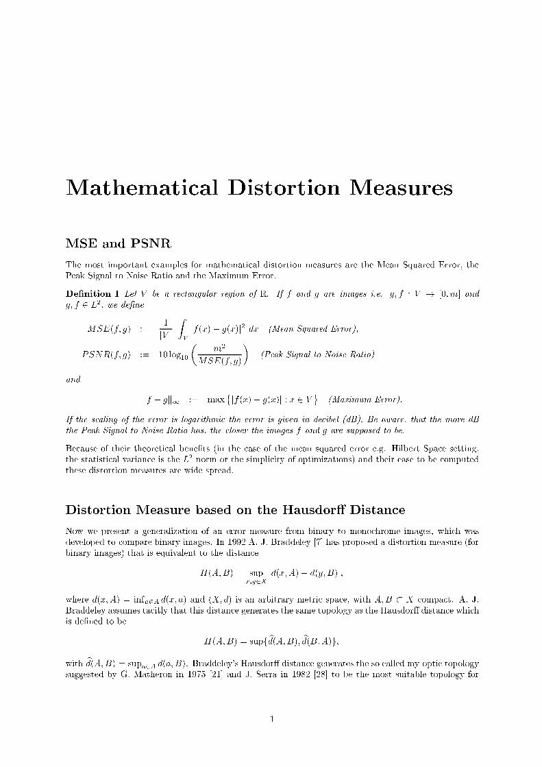
Mathematical Distortion Measures
MSE and PSNR
The most important examples for mathematical distortion measures are the Mean Squared Error, the
Peak Signal to Noise Ratio and the Maximum Error.
De�nition 1 Let V be a rectangular region of R. If f and g are images i.e. g; f : V ! [0;m] and
g; f 2 L2, we de�ne
MSE(f; g) :=1
jV j
ZV
jf(x)� g(x)j2 dx (Mean Squared Error),
PSNR(f; g) := 10 log10
�m2
MSE(f; g)
�(Peak Signal to Noise Ratio)
and
kf � gk1 := max�jf(x)� g(x)j : x 2 V
(Maximum Error).
If the scaling of the error is logarithmic the error is given in decibel (dB). Be aware, that the more dB
the Peak Signal to Noise Ratio has, the closer the images f and g are supposed to be.
Because of their theoretical bene�ts (in the case of the mean squared error e.g. Hilbert Space setting,
the statistical variance is the L2 norm or the simplicity of optimizations) and their ease to be computed
these distortion measures are wide spread.
Distortion Measure based on the Hausdor� Distance
Now we present a generalization of an error measure from binary to monochrome images, which was
developed to compare binary images. In 1992 A. J. Braddeley [7] has proposed a distortion measure (for
binary images) that is equivalent to the distance
H(A;B) = supx;y2X
jd(x;A)� d(y;B)j;
where d(x;A) = infa2A d(x; a) and (X; d) is an arbitrary metric space, with A;B � X compact. A. J.
Braddeley assumes tacitly that this distance generates the same topology as the Hausdor� distance which
is de�ned to be
H(A;B) = supfbd(A;B); bd(B;A)g;with bd(A;B) = supa2A d(a;B). Braddeley's Hausdor� distance generates the so called my-optic topology
suggested by G. Matheron in 1975 [21] and J. Serra in 1982 [28] to be the most suitable topology for
1
binary image comparisons. A. J. Braddeley changes the Hausdor� distance and bounds the result by a
constant c:
�binary(A;B) =
(1
jX jXx2X
jd�(x;A)� d�(x;B)jp) 1
p
;
with 1 � p < 1 and d�(x;A) = minfinfa2A d(x;A); cg. The constant c ensures that no points farther
than c "pixels" away from the sets A or B contribute to the numerical value of the metric. The parameter
p controls the relative weight of errors of di�erent magnitude and for p ! 1 the metric �binary(A;B)tends towards the Hausdor� metric.
Of course, this concept of a binary image comparison can be generalized to a new image metric for grey
scale images as it was done by D. L. Wilson, A. J. Braddeley and R. A. Owens in 1997 [36]. They
regarded the distance of two images f and g to be the distance from the graph of f to the graph of ginterpreted as sets. According to Matheron (1975) [21] the subgraph of an image f : X ! Y � R is
de�ned as �f = f(x; y) : x 2 X; y 2 Y with y � f(x)g. A metric de�ned on the class of all continuous
subgraphs generates a topology know as the sup vague topology, �rst introduced by W. Vervaat in 1988
[34]. The de�nition of the distance between the graphs of images is derived as follows: De�ne a metric
on the space X � Y as
d((x; y); (x0; y0)) = maxfd(x; x0); jy � y0jg:
This was chosen out of many other possibilities because of the ease of computation in practical applica-
tions. For an image de�ne the upper level set as Xy = fx 2 X : f(x) � yg, whereas y is a grey level
intensity and set the distance from a point x 2 X to the upper level set Xy to be
d(x;Xy(f)) = infx02Xy(f)
d(x; x0):
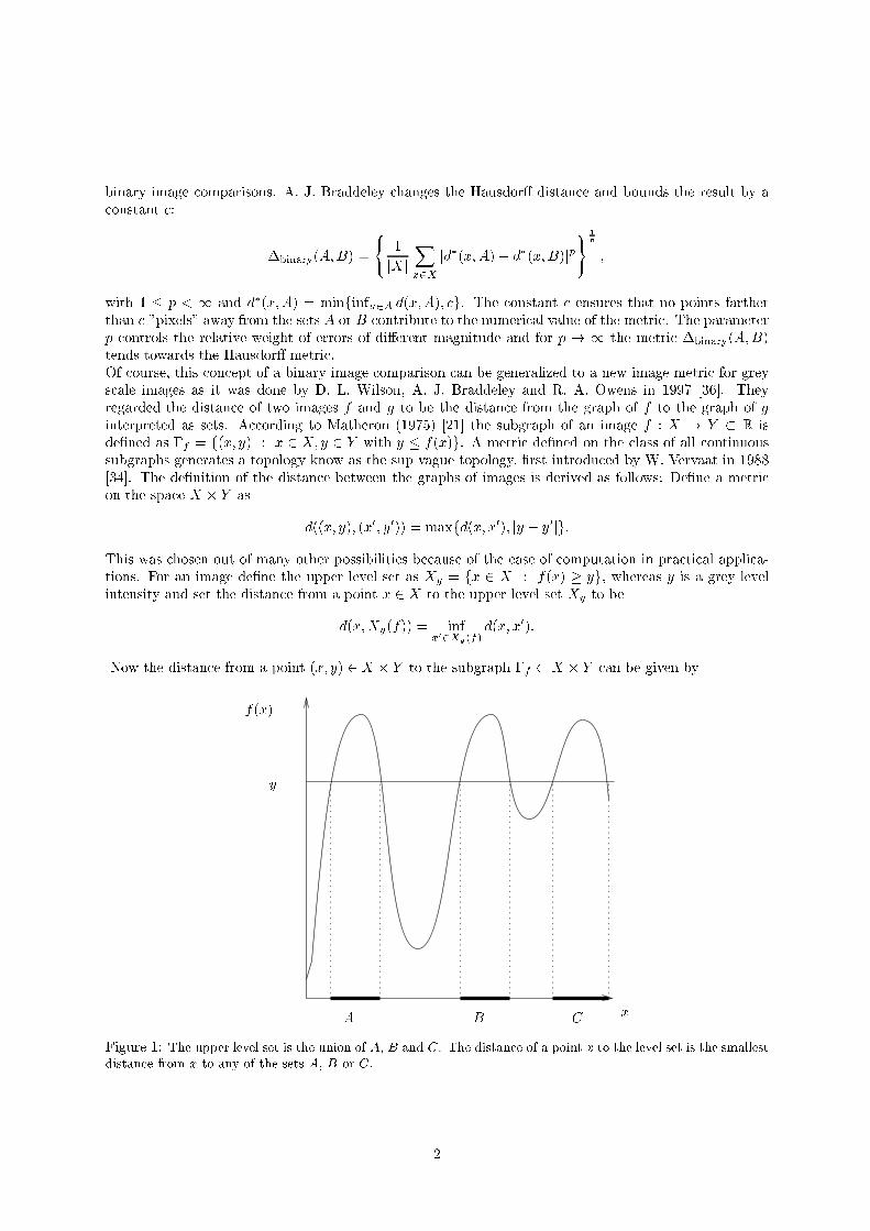
Now the distance from a point (x; y) 2 X � Y to the subgraph �f � X � Y can be given by
f(x)
x
y
A B C
Figure 1: The upper level set is the union of A, B and C. The distance of a point x to the level set is the smallest
distance from x to any of the sets A, B or C.
2
d((x; y);�f ) = inf�d�(x; y); (x0; y0)
�: (x0; y0) 2 �f
= inf
y02Y
�inf
x02Xy0 (f)
�max
�d(x; x0); jy � y0j
��= inf
y02Y
�maxf inf
x02Xy0 (f)
fd(x; x0); jy � y0jgg�
= infy02Y
fmax fd(x;Xy0(f)); jy � y0jgg :
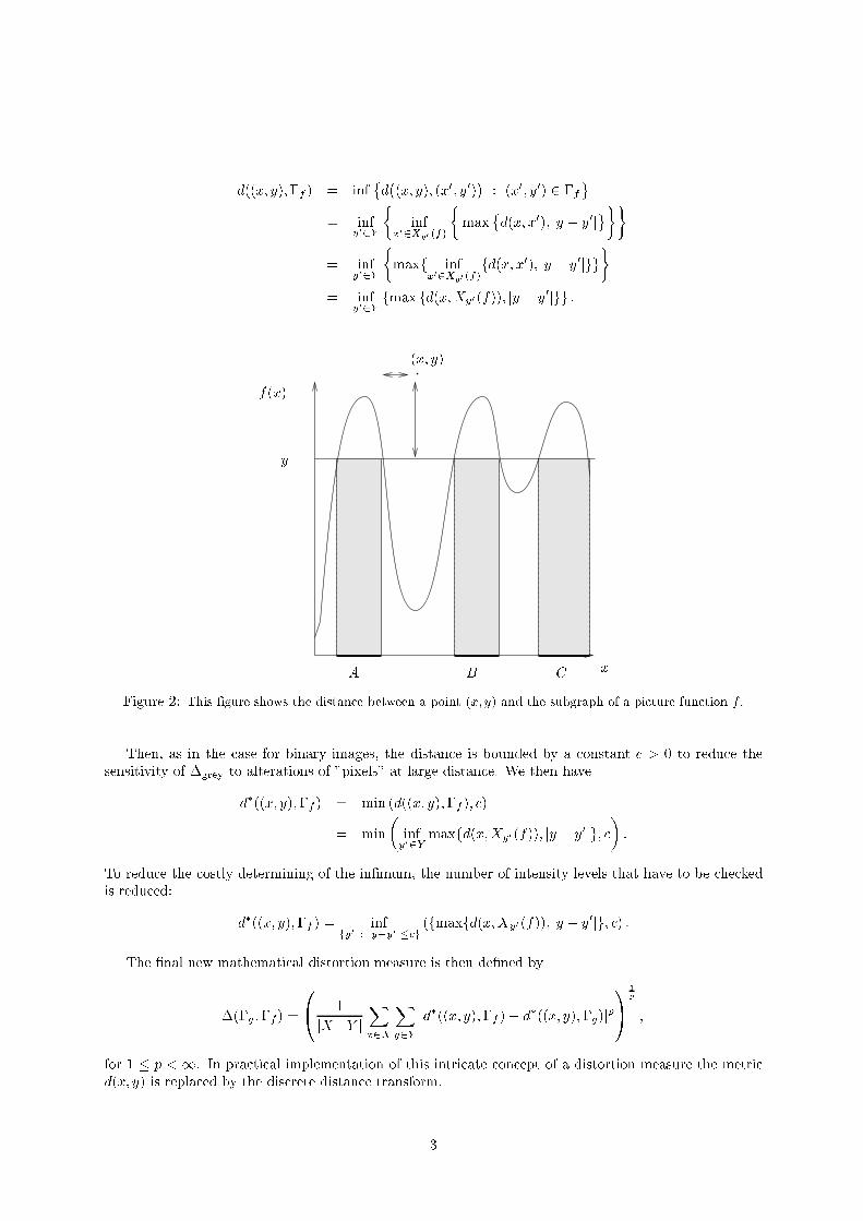
.
f(x)
x
y
A B C
(x; y)
Figure 2: This �gure shows the distance between a point (x; y) and the subgraph of a picture function f .
Then, as in the case for binary images, the distance is bounded by a constant c > 0 to reduce the
sensitivity of �grey to alterations of "pixels" at large distance. We then have
d�((x; y);�f ) = min (d((x; y);�f ); c)
= min
�infy02Y
maxfd(x;Xy0(f)); jy � y0jg; c�:
To reduce the costly determining of the in�mum, the number of intensity levels that have to be checked
is reduced:
d�((x; y);�f ) = inffy0 : jy�y0j�cg
(fmaxfd(x;Xy0(f)); jy � y0jg; c) :
The �nal new mathematical distortion measure is then de�ned by
�(�g ;�f ) =
0@ 1
jX j jY jXx2X
Xy2Y
jd�((x; y);�f )� d�((x; y);�g)jp1A
1
p
;
for 1 � p < 1. In practical implementation of this intricate concept of a distortion measure the metric
d(x; y) is replaced by the discrete distance transform.
3
Discussion
It has long been accepted that the MSE and PSNR measures are inaccurate in predicting a reasonable
correspondence with the subjective evaluation of an observer or interpreter of an image. In the context of
image compression, there is at most at high and medium bit rate a correlation between the image quality
and the above introduced measures.
Remember, that
bit rate =bits
pixel
compressed image size
original image size:
In the following we are going to explain a scheme of how to construct images with qualities that are not
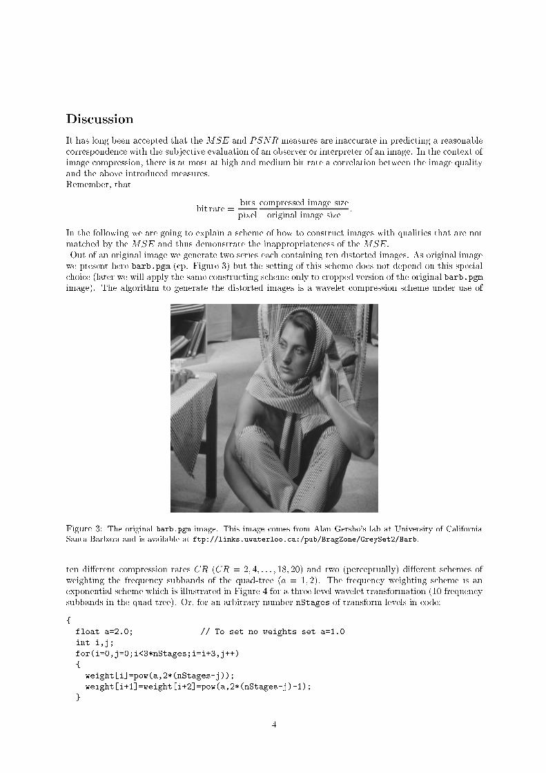
matched by the MSE and thus demonstrate the inappropriateness of the MSE.Out of an original image we generate two series each containing ten distorted images. As original image
we present here barb.pgm (cp. Figure 3) but the setting of this scheme does not depend on this special
choice (later we will apply the same constructing scheme only to cropped version of the original barb.pgm
image). The algorithm to generate the distorted images is a wavelet compression scheme under use of
Figure 3: The original barb.pgm image. This image comes from Alan Gersho's lab at University of California
Santa Barbara and is available at ftp://links.uwaterloo.ca:/pub/BragZone/GreySet2/Barb.
ten di�erent compression rates CR (CR = 2; 4; : : : ; 18; 20) and two (perceptually) di�erent schemes of
weighting the frequency subbands of the quad-tree (a = 1; 2). The frequency weighting scheme is an
exponential scheme which is illustrated in Figure 4 for a three level wavelet transformation (10 frequency
subbands in the quad-tree). Or, for an arbitrary number nStages of transform levels in code:
{
float a=2.0; // To set no weights set a=1.0
int i,j;
for(i=0,j=0;i<3*nStages;i=i+3,j++)
{
weight[i]=pow(a,2*(nStages-j));
weight[i+1]=weight[i+2]=pow(a,2*(nStages-j)-1);
}
4
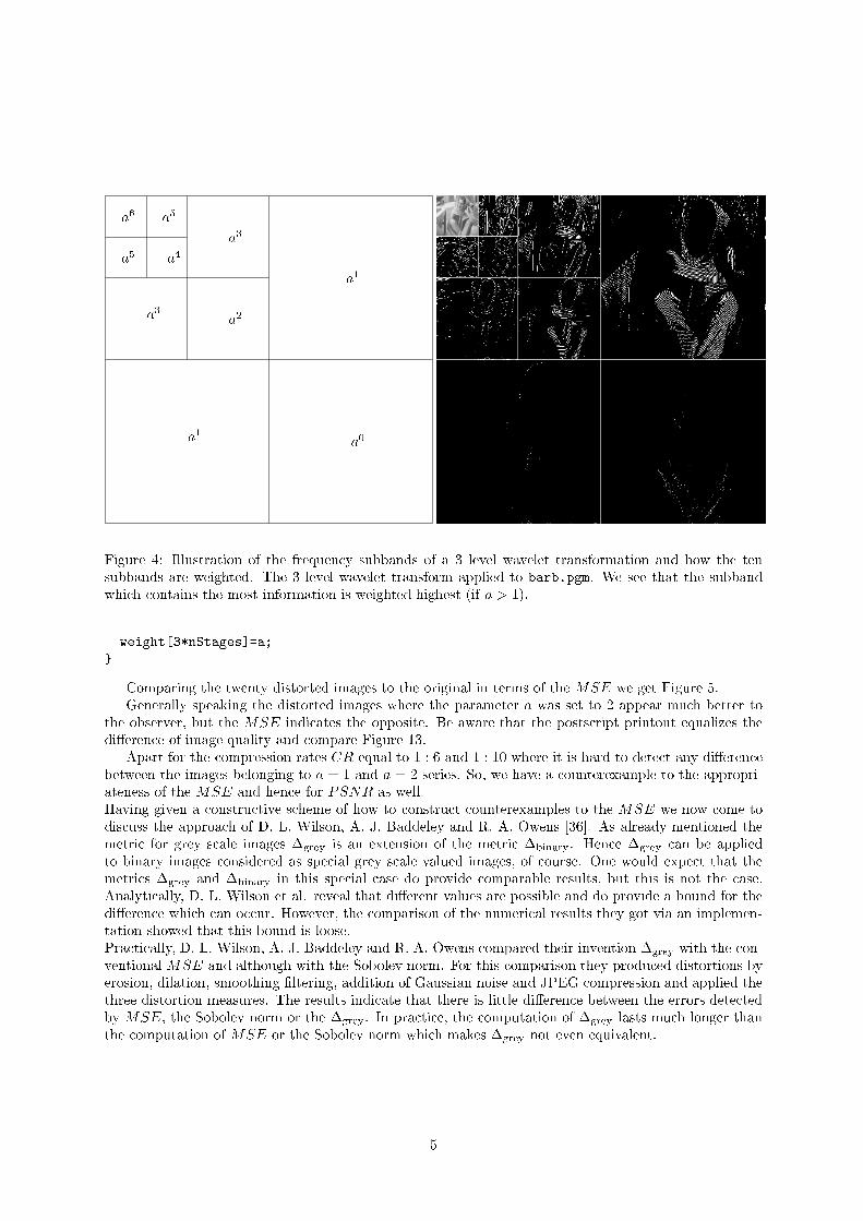
a0a1
a1
a2a3
a3
a4a5
a5a6
Figure 4: Illustration of the frequency subbands of a 3 level wavelet transformation and how the ten
subbands are weighted. The 3 level wavelet transform applied to barb.pgm. We see that the subband
which contains the most information is weighted highest (if a > 1).
weight[3*nStages]=a;
}
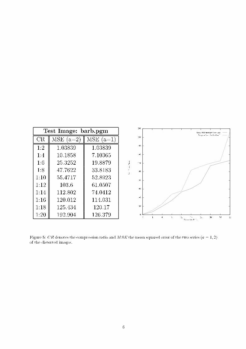
Comparing the twenty distorted images to the original in terms of the MSE we get Figure 5.
Generally speaking the distorted images where the parameter a was set to 2 appear much better to
the observer, but the MSE indicates the opposite. Be aware that the postscript printout equalizes the
di�erence of image quality and compare Figure 13.
Apart for the compression rates CR equal to 1 : 6 and 1 : 10 where it is hard to detect any di�erence
between the images belonging to a = 1 and a = 2 series. So, we have a counterexample to the appropri-
ateness of the MSE and hence for PSNR as well.
Having given a constructive scheme of how to construct counterexamples to the MSE we now come to
discuss the approach of D. L. Wilson, A. J. Baddeley and R. A. Owens [36]. As already mentioned the
metric for grey scale images �grey is an extension of the metric �binary. Hence �grey can be applied
to binary images considered as special grey scale valued images, of course. One would expect that the
metrics �grey and �binary in this special case do provide comparable results, but this is not the case.
Analytically, D. L. Wilson et al. reveal that di�erent values are possible and do provide a bound for the
di�erence which can occur. However, the comparison of the numerical results they got via an implemen-
tation showed that this bound is loose.
Practically, D. L. Wilson, A. J. Baddeley and R. A. Owens compared their invention �grey with the con-
ventional MSE and although with the Sobolev norm. For this comparison they produced distortions by
erosion, dilation, smoothing �ltering, addition of Gaussian noise and JPEG compression and applied the
three distortion measures. The results indicate that there is little di�erence between the errors detected
by MSE, the Sobolev norm or the �grey. In practice, the computation of �grey lasts much longer than
the computation of MSE or the Sobolev norm which makes �grey not even equivalent.
5
Test Image: barb.pgm
CR MSE (a=2) MSE (a=1)
1:2 1.03839 1.03839
1:4 10.1858 7.10365
1:6 25.3252 19.8879
1:8 47.7622 33.8183
1:10 55.4717 52.8923
1:12 103.6 61.0507
1:14 112.802 74.0412
1:16 120.012 114.031
1:18 125.434 120.17
1:20 192.904 126.379
200
180
160
140
120
100
80
60
40
0
Compression Ratio
MeanSquareError
2 4 6 8 10 12 14 16 18 20
20
Image with unweighted subbands
Image with weighted subbands
Figure 5: CR denotes the compression ratio andMSE the mean squared error of the two series (a = 1; 2)
of the distorted images.
6
Distortion Measures In-cooperating
the Human Visual System or
Imaging Device
As we already saw in the last discussion there is a need to derive new distortion measures from an
acceptable visual system model. Here in the present section we will present an overview over the
attempts which have been undertaken on this subject in the past decades.
The Spatial Fourier CoeÆcients Weighted Approach
Due to our knowledge the very �rst attempt was undertaken by William A. Pearlman, in 1977 [25]. The
reasons governing his choice of a weighted squared error are the following:
1. squared error is the commonly used criterion for image processing,
2. any newly proposed criterion must establish its superiority over squared error in some respect,
3. demonstrated superiority of the new criterion over squared error would strongly suggest it as a
more accurate model of the system's performance change under intensity variation, and
4. the mathematical properties of the new criterion point naturally to squared error for comparison.
5. Rate distortion algorithms are often justi�ed strictly only for distortion measures provided the
distortion measure for the code blocks is additive. This additive property is is satis�ed by MSE or
frequency weighted MSE.
His new criterion is an amplitude{weighted, absolute squared di�erence in the spatial Fourier coef-
�cients of the image, not to be confused with a common index{weighted measure of the of the formPj wj cj , if cj are the Fourier coeÆcients.Pearlman's new distortion measure is derived from A. D. Schnitzler's [27] model of the human visual
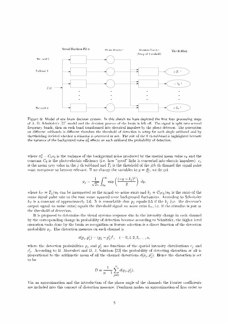
system, which consists of four basic steps: The incident light is a�ected by the optical system of the eye
consisting of the lens and the pupil, which are de�ning a modulation function. The retinal elements are
image sensors which may be regarded as photo cells where the incident photons of light are absorbed
and converted into electrical impulses. The electrical impulses are transmitted to the brain and �nally
the brain processes the electrical impulses. In this model, Pearlman does envision the human eye{brain
system as a bank of parallel, narrow band �lters each tuned to a di�erent spatial frequency. For an
illustration see Figure 6. The probability of detection of a complex object is the sum of the probabilities
of detection in each channel, consistent with the assumption of channel independence and the detection
results of H. Mostafavi and D. J. Sakrison [22]. The probability of detecting an error in the jth frequencysubband is
pj =1p2�
Z 1
Tj
1
j�0jexp
�� (x� C0cj)
2
(2�20)
�dx;
7
.
.
....
.
.
....
Subband 0
Subband 1
Subband n
f(x)
Spatial Bandpass Filter Photo Detector Decision Counter
(Setup of Threshold)Thresholding
> T1 ?
> T2 ?
> Tn ?
Figure 6: Model of eye{brain decision system. In this sketch we have depicted the �rst four processing steps
of A. D. Schnitzler's [27] model and the decision process of the brain is left o�. The signal is split into severalfrequency bands, then on each band transformed into electrical impulses by the photo detector. The perceptionon di�erent subbands is di�erent therefore the threshold of detection is setup for each single subband and by
thresholding decided whether a stimulus is perceived or not. The role of the 0 th subband is highlighted becausethe variance of the background noise �20 e�ects on each subband the probability of detection.
where �20 = C0c0 is the variance of the background noise produced by the spatial mean value c0 and the
constant C0 is the photo-electric eÆciency (i.e. how "good" light is converted into electric impulses). cjis the mean grey value in the j th subband and Tj is the threshold of the jth th channel the signal pulse
must overpower to become relevant. If we change the variables to y = x�0, we do get
pj =1p2�
Z 1
kT
exp
�(�y � kj)
2
2
�dy;
where kT = Tj=�0 can be interpreted as the signal{to{noise{ratio and kj = C0cj=�0 is the ratio of the
mean signal pulse rate to the root mean squared error background uctuation. According to Schnitzler
kT is a constant of approximately 2:6. It is remarkable that pj equals 0:5 if the kj (i.e. the detector's
output signal{to{noise{ratio) equals the threshold signal{to{noise ratio kT , i.e. if the stimulus is just atthe threshold of detection.
It is proposed to determine the visual systems response due to the intensity change in each channel
by the corresponding change in probability of detection because according to Schnitzler, the higher level
operation tasks done by the brain as recognition or feature selection is a direct function of the detection
probability pj . The distortion measure on each channel is
d(pj ; p0
j) = (pj � p0j)2; i = 0; 1; 2; 3; : : : ; n;
where the detection probabilities pj and p0j are functions of the spatial intensity distributions cj and
c0j . According to H. Mostafavi and D. J. Sakrison [22] the probability of detecting distortion at all is
proportional to the arithmetic mean of all the channel distortions d(pj ; p0j). Hence the distortion is set
to be
D =1
n+ 1
nXj=0
d(pj ; p0
j):
Via an approximation and the introduction of the phase angle of the channels the Fourier coeÆcients
are included into this concept of distortion measure. Pearlman makes an approximation of �rst order to
8
make the resulting distortion measure more handy:
d(p(cj); p(c0
j)) = (pj � p0j)2
��@p
@cj(cj � c0j)
�2
=1
2�c20exp
��(kT � kj)
2� ��cj � c0j
��2=
1
2�c20exp
��kT �
C0
�0cj
�2!
| {z }=:w(cj)
��cj � c0j��2 :
Remind, that until now this concept of a distortion measure does not involve the phase angle of the
subbands at all. However, performing the decision process the brain has to synthesize the set of subband
information and thus does involve the phase angle. Pearlman does compose the scalar product
aj =
ZR
cj exp(i�j) d� and a0j =
ZR
c0j exp(i�0
j) d�:
Because of
jcj � c0j j � jaj � a0j j
we can simply substitute cj by aj and get �nally as the total distortion
D � 1
n+ 1
nXj=0
w(aj)��aj � a0j
��2 ;where the weighting function w(�) depends not only on the index j of the Fourier coeÆcients of the
original image, but although on their amplitude.
Invariant Power Spectrum Approach
This approach was developed by N. B. Nill and B. H. Bouzas in 1991 [23]. As in the case of the spatial
Fourier coeÆcients weighted methods, the following foundation of a distortion measure will depend on
the Fourier coeÆcients, too. However, the major di�erence to any other approach is the assumption that
the power spectrum of an image is invariant under the change of scale. This assumption guarantees N. B.
Nill and B. H. Bouzas an invariant entity which makes it possible to assign each single image a number
of quality. All other approaches compare two images and measure the di�erence.
The assumption that the power spectra of natural scenes are one and the same is justi�ed according to
N. B. Nill and B. H. Bouzas due to a fundamental order in natural scene, namely by the fractal structure.
Without such an assumption there would be a lack of a constant entity necessary to assign a single image
with an image quality measure, of course.
The power spectrum of an image f(x) is de�ned as j bf(!)j2, when bf(!) is the Fourier transformationof the image. To compensate the e�ect of brightness variation from image to image the power spectrum
is normalized by the mean grey value � of the image. Of course, the power spectrum also depends on
the number of pixels jV j contained in the image, so that one also has to divide by the number of pixels
which results in
P (!) =j bf(!)j2�2jV j :
This normalized power spectrum P (!) is used to separate the image into parts, where the image infor-
mation is concentrated because by N. B. Nill and B. H. Bouzas human observers are supposed to ignore
9
uniform large regions and base their subjective quality ratings on the structured regions. The larger an
uniform image region is involved in the consideration the less signi�cant is their IQM (Image Quality
Measure).
The human visual system is invoked in this approach to a distortion measure by the work of J. L.
Mannos and D. J. Sakrison [20] as well as by the work of J. J. DePalma and E. M. Lowry [11]: the human
visual system acts as a bandpass �lter with the impulse response
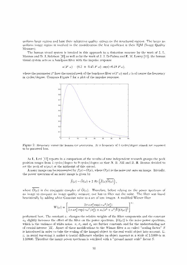
w(P !) = (0:2 + 0:45 P !) exp(�0:18 P !);
where the parameter P �xes the spatial peek of the bandpass �lter w(P !) and ! is of course the frequency
in cycles/degree. Compare Figure 7 for a plot of the impulse response.
0 5 10 15 20 25 30 35 400
0.1
0.2
0.3
0.4
0.5
0.6
0.7
0.8
0.9
1
Figure 7: Frequency versus the human eye perception. At a frequency of 5 cycles/degree stimuli are supposed
to be perceived best.
As L. Levi [17] reports in a comparison of the results of nine independent research groups the peek
position ranges from 1 cycles/degree to 9 cycles/degree so that N. B. Nill and B. H. Bouzas decided to
set the peek of w(p!) at the midpoint of this spread.A noisy image can be represented by f(x)+O(x), where O(x) is the noise put onto an image. Trivially,
the power spectrum of an noisy image is given by
bf(!) + bO(!) + 2 Re�bf(!) bO(!)� ;
where bO(!) is the conjugate complex of bO(!). Therefore, before relying on the power spectrum of
an image to compute an image quality measure, one has to �lter out the noise. The �lter was found
heuristically by adding white Gaussian noise to a set of test images. A modi�ed Wiener �lter
W (!) =
"2� a �2s exp(�!2=�2g)
2� a�2s exp(�!2=�2g) + �1(a2 + !2)3
2 jO(!)j2
#�2performed best. The constant �1 changes the relative weights of the �lter components and the constant
�2 slightly increases the e�ect of the �lter on the power spectrum. jO(!)j is the noise power spectrum,which is the variance of white noise. a, �s and �g are further constants and for the understanding not
of crucial interest [23]. Apart of these modi�cations to the Wiener �lter a so called "scaling factor" Sis introduced in order to take the scaling of the imaged object to the real world object into account. E.
g. in aerial surveying it makes a crucial di�erence whether an object appears at a scale of 1:1000 or at
1:10000. Therefore the image power spectrum is weighted with a "ground image scale" factor S.
10
From these di�erent aspects the IQM is derived from the normalized power spectrum, weighted by the
square of modulation transfer function of the human visual system w(!) and the scale factor S, �lteredwith the Wiener �lter W (!):
IQM =1
jV j
Z +�
��
Z 1
2
1
100
P (!) W (!) w2(!)S(!;�) d! d�:
The integration boundaries are explained by heuristics and are not of general importance.
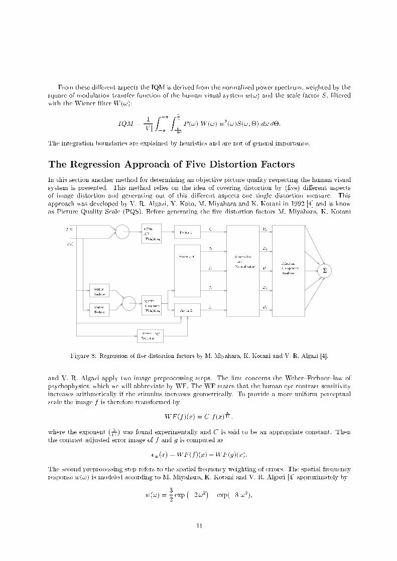
The Regression Approach of Five Distortion Factors
In this section another method for determining an objective picture quality respecting the human visual
system is presented. This method relies on the idea of covering distortion by (�ve) di�erent aspects
of image distortion and generating out of this di�erent aspects one single distortion measure. This
approach was developed by V. R. Algazi, Y. Kato, M. Miyahara and K. Kotani in 1992 [4] and is know
as Picture Quality Scale (PQS). Before generating the �ve distortion factors M. Miyahara, K. Kotani
Σ
f(x)
g(x)
Weber
Weber
Fechner
Fechner
CCIR
567{1
Weighting
Weighting
Spatial
Frequency
Kirsch Edge
Detection
Factor 1
Factor 2{4
Factor 5
Summation
and
NormalizationPrincipal
Component
Analysis
{
{
D1
D2
D3
D4
D5
f1
f2
f3
f4
f5
Figure 8: Regression of �ve distortion factors by M. Miyahara, K. Kotani and V. R. Algazi [4].
and V. R. Algazi apply two image preprocessing steps. The �rst concerns the Weber{Fechner{law of
psychophysics, which we will abbreviate by WF. The WF states that the human eye contrast sensitivity
increases arithmetically if the stimulus increases geometrically. To provide a more uniform perceptual
scale the image f is therefore transformed by
WF (f)(x) = C f(x)5
11 ;
where the exponent ( 511) was found experimentally and C is said to be an appropriate constant. Then
the contrast adjusted error image of f and g is computed as
ew(x) =WF (f)(x)�WF (g)(x):
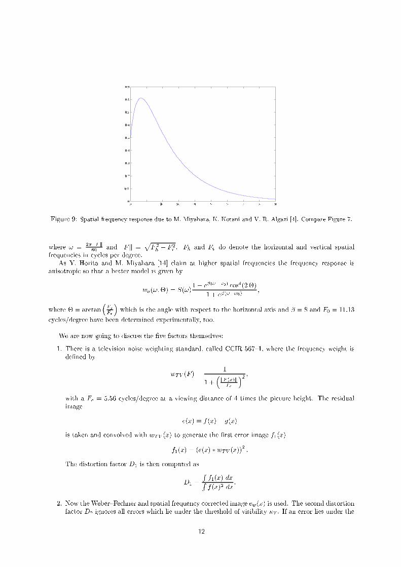
The second preprocessing step refers to the spatial frequency weighting of errors. The spatial frequency
response w(!) is modeled according to M. Miyahara, K. Kotani and V. R. Algazi [4] approximately by
w(!) =3
2exp
��2!2
�� exp(�8 !2);
11
0.9
0.8
0.7
0.6
0.5
0.4
0.3
0.2
0.1
00 10 20 30 40 5 6 7 8 9
Figure 9: Spatial frequency response due to M. Miyahara, K. Kotani and V. R. Algazi [4]. Compare Figure 7.
where ! =2� kFk
60and kFk =
pF 2h + F 2
v . Fh and Fv do denote the horizontal and vertical spatial
frequencies in cycles per degree.
As Y. Horita and M. Miyahara [14] claim at higher spatial frequencies the frequency response is
anisotropic so that a better model is given by
wa(!;�) = S(!)1 + e�(!�!0) cos4(2�)
1 + e�(!�!0);
where � = arctan�FyFx
�which is the angle with respect to the horizontal axis and � = 8 and F0 = 11:13
cycles/degree have been determined experimentally, too.
We are now going to discuss the �ve factors themselves:
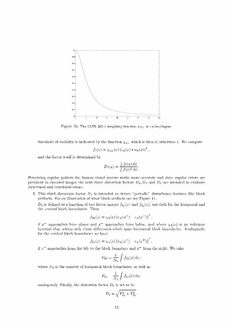
1. There is a television noise weighting standard, called CCIR 567{1, where the frequency weight is
de�ned by
wTV (F ) =1
1 +�kF (x)k
Fc
�2 ;with a Fc = 5:56 cycles/degree at a viewing distance of 4 times the picture height. The residual
image
e(x) = f(x)� g(x)
is taken and convolved with wTV (x) to generate the �rst error image f1(x)
f1(x) = (e(x) � wTV (x))2 :
The distortion factor D1 is then computed as
D1 =
Rf1(x) dxRf(x)2 dx
:
2. Now the Weber{Fechner and spatial frequency corrected image ew(x) is used. The second distortionfactor D2 ignores all errors which lie under the threshold of visibility �T . If an error lies under the
12
1
0.9
0.8
0.7
0.6
0.5
0.4
0.3
0.2
0.1
00 10 15 20 25 30 35 405
Figure 10: The CCIR 567-1 weighting function wTV in cycles/degree.
threshold of visibility is indicated by the function ��T which is then 0, otherwise 1. We compute
f2(x) = ��T (x) (ew(x) � wa(x))2 ;
and the factor itself is determined by
D2(x) =
Rf2(x) dxRf(x)2 dx
:
Perceiving regular pattern the human visual system works more accurate and since regular errors are
prevalent in encoded images the next three distortion factors D3; D4 and D5 are intended to evaluate
structured and correlated errors.
3. This third distortion factor D3 is intended to detect "periodic" disturbance features like block
artifacts. For an illustration of what block artifacts are see Figure 11.
D3 is de�ned as a function of two factor images f3h(x) and f3v(x), one each for the horizontal and
the vertical block boundaries. Thus,
f3h(x) = �h(x)�ew(x
�)� ew(x+)�2;
if x� approaches from above and x+ approaches from below, and where �h(x) is an indicator
function that selects only those di�erences which span horizontal block boundaries. Analogously
for the vertical block boundaries we have
f3v(x) = �v(x)�ew(x
�)� ew(x+)�2;
if x� approaches from the left to the block boundary and x+ from the right. We take
F3h =1
Nh
Zf3h(x) dx;
where Nh is the number of horizontal block boundaries, as well as
F3v =1
Nv
Zf3v(x) dx;
analogously. Finally, the distortion factor D3 is set to be
D3 =
qF 23v + F 2
3h:
13
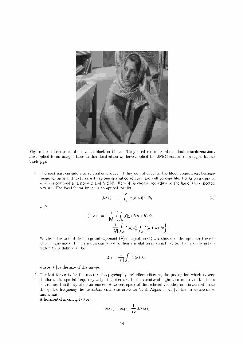
Figure 11: Illustration of so called block artifacts. They used to occur when block transformations
are applied to an image. Here in this illustration we have applied the JPEG compression algorithm to
barb.pgm.
4. The next part considers correlated errors even if they do not occur at the block boundaries, because
image features and textures with strong spatial correlation are well perceptible. Let Q be a square,
which is centered at a point x and h 2 W . Here W is chosen according to the lag of the expected
texture. The local factor image is computed locally
f4(x) =
ZW
jr(x; h)j 14 dh; (1)
with
r(x; h) =1
jQj
�ZQ
f(y) f(y + h) dy
� 1
jQj
ZQ
f(y) dy
ZQ
f(y + h) dy
�:
We should note that the integrand exponent�14
�in equation (1) was chosen to deemphasize the rel-
ative magnitude of the errors, as compared to their correlation or structure. So, the next distortion
factor D4 is de�ned to be
D4 =1
jV j
ZV
f4(x) dx;
where jV j is the size of the image.
5. The last factor is for the matter of a psychophysical e�ect a�ecting the perception which is very
similar to the spatial frequency weighting of errors: in the vicinity of hight contrast transition there
is a reduced visibility of disturbances. However, apart of the reduced visibility and interrelation to
the spatial frequency the disturbances in this areas for V. R. Algazi et al. [4] this errors are most
important.
A horizontal masking factor
Sh(x) = exp(� 1
25Mh(x))
14
was introduced by J. O. Limb in 1979 [18] in terms of a horizontal local contrast activity function
Mh(x) =1
2
���f(x�)� f(x+)���:
Analogously, we de�ne the vertical local contrast activity function Sv(x). The masked error at the
pixel x is then computed as
f5(x) = �M (x) jew(x)j (Sh(x) + Sv(x));
where the function �M (x) is an indicator function which selects the pixels "close" to high intensity
transitions. The �nal factor D5 is then computed as
D5 =1
N
Zf5(x) dx;
where N is now the number of pixels chosen to have high intensity transitions. This choice is done
using the response of the Kirsch edge [16] detection operator.
The factors D1; : : : ; D5 have been de�ned to evaluate di�erent speci�c types of impairment. It is
obvious that some of the local image distortions will contribute to several of the factors or to all of the
factors: the factors D1; : : : ; D5 are correlated. E.g. there is a multiple frequency weighting (CCIR 567-1
and Mannos and Sakrison [20]) as well as a multiple coverage of correlated errors (block artifacts and
other structured disturbances). To carry out these multiple coverages an "principal component analysis"
is done by computing the covariance matrix
CD = E�( ~D � �D)( ~D � �D)
T;
where E is the matrix of eigenvectors to diagonalize the matrix ( ~D � �D)( ~D � �D)T with ~D =
(D1; D2; : : : ; D5) and the entries of vector �D are the arithmetic means of the distortion factors Di
of the set of images to which the objective picture quality scale will be applied. The eigenvalues �iindicate the relative contribution of the corresponding distortion factor Di to the total distortion and
are uncorrelated. Now the more important components are chosen and ultimately the objective picture
quality scale for image coding is derived by an linear combination of these principal components.
Discussion and Examples
In this section we take the opportunity to give the PQS approach a practical trial. A more thorough
evaluation can be found in the original papers [3] and [4]. We use the PQS implementation provided by
R. Estes and V. R. Algazi [12]. We cropped a window of size 256 starting at the pixel (192; 0) out of theoriginal barb.pgm image (cp. Figure 3 and Figure 13). We have to do so, because the implementation
provided by R. Estes and V. R. Algazi handles only images of this size. Out of this clip we generated
two series of images (cp. Figure 13) according to the scheme we already described on page 4.
It is remarkable, that PQS 6= 0 even if we compare two identical images. Here in this example, the
original barbface.pgm image compared with itself one gets PQS = 5:79 and the closer the PQS is to
this value the better are the reconstructed images supposed to be. Apart of the fact that the PQS is an
engineering approach it lacks at speediness of the computation. Theoretically, there are little chances to
study the PQS mathematically to optimize routines for this distortion measure.
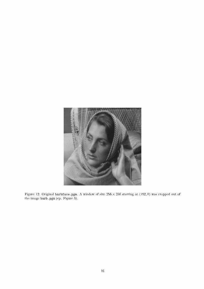
Figure 12: Original barbface.pgm. A window of size 256� 256 starting at (192; 0) was cropped out of
the image barb.pgm (cp. Figure 3).
16
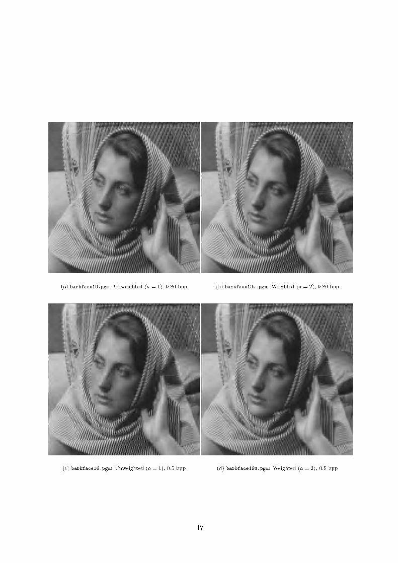
(a) barbface10.pgm: Unweighted (a = 1), 0:80 bpp (b) barbface10w.pgm: Weighted (a = 2), 0:80 bpp
(c) barbface16.pgm: Unweighted (a = 1), 0:5 bpp (d) barbface16w.pgm: Weighted (a = 2), 0:5 bpp
17
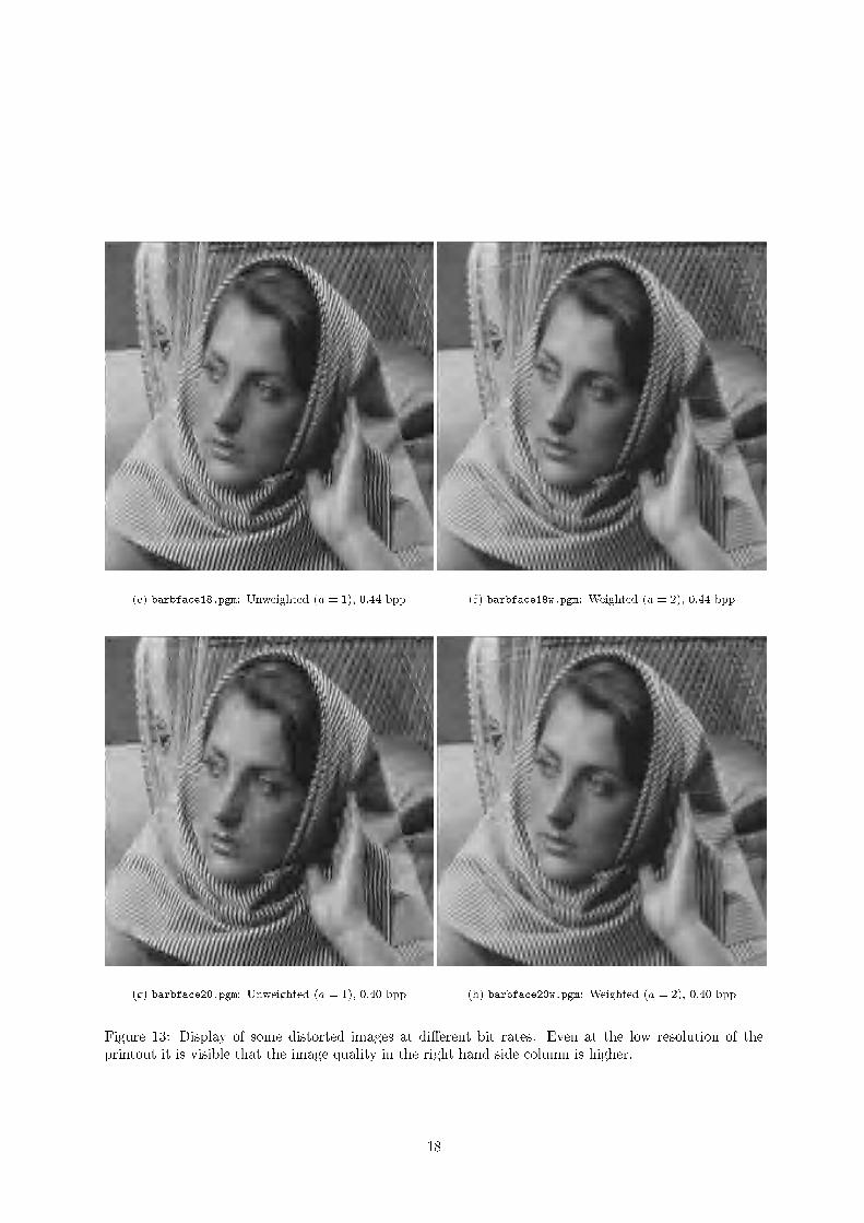
(e) barbface18.pgm: Unweighted (a = 1), 0:44 bpp (f) barbface18w.pgm: Weighted (a = 2), 0:44 bpp
(g) barbface20.pgm: Unweighted (a = 1), 0:40 bpp (h) barbface20w.pgm: Weighted (a = 2), 0:40 bpp
Figure 13: Display of some distorted images at di�erent bit rates. Even at the low resolution of the
printout it is visible that the image quality in the right hand side column is higher.
18
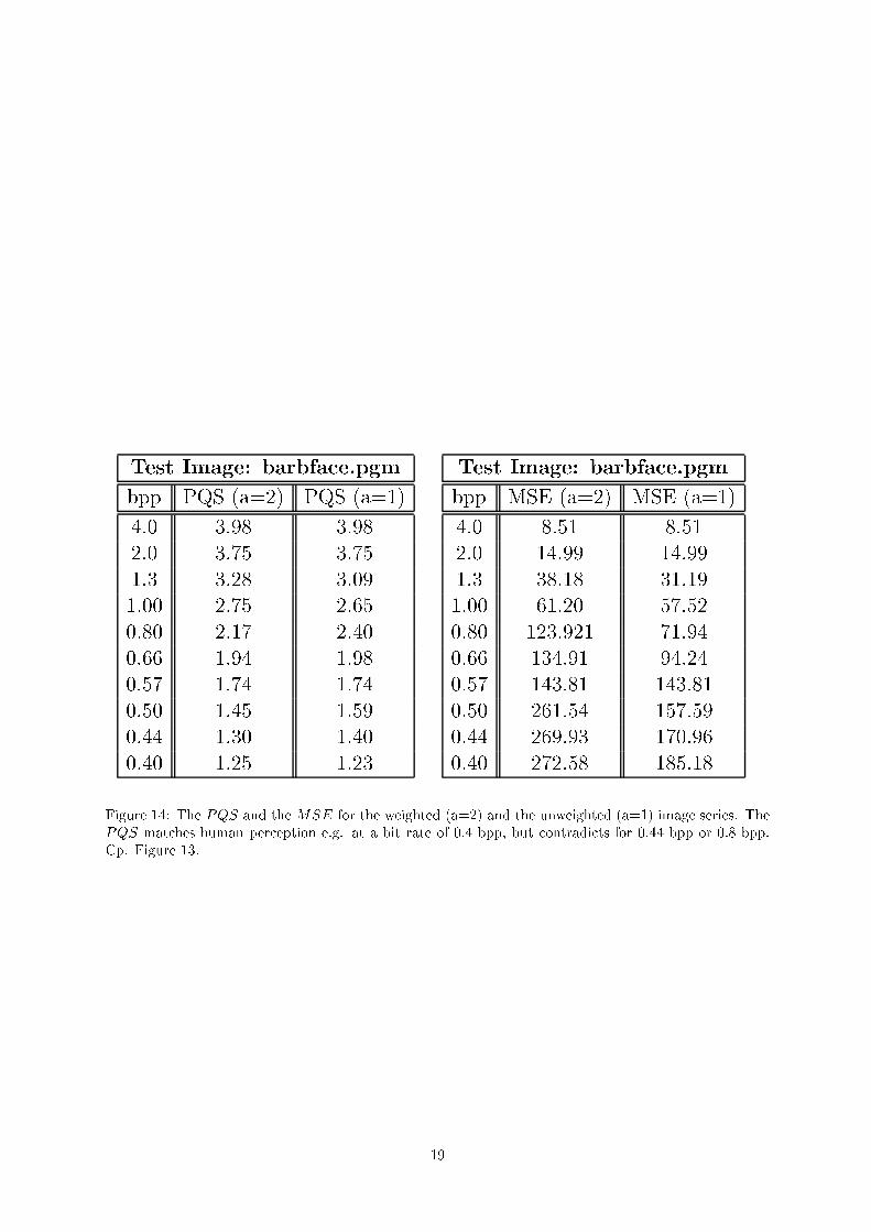
Test Image: barbface.pgm
bpp PQS (a=2) PQS (a=1)
4.0 3.98 3.98
2.0 3.75 3.75
1.3 3.28 3.09
1.00 2.75 2.65
0.80 2.17 2.40
0.66 1.94 1.98
0.57 1.74 1.74
0.50 1.45 1.59
0.44 1.30 1.40
0.40 1.25 1.23
Test Image: barbface.pgm
bpp MSE (a=2) MSE (a=1)
4.0 8.51 8.51
2.0 14.99 14.99
1.3 38.18 31.19
1.00 61.20 57.52
0.80 123.921 71.94
0.66 134.91 94.24
0.57 143.81 143.81
0.50 261.54 157.59
0.44 269.93 170.96
0.40 272.58 185.18
Figure 14: The PQS and the MSE for the weighted (a=2) and the unweighted (a=1) image series. The
PQS matches human perception e.g. at a bit rate of 0:4 bpp, but contradicts for 0:44 bpp or 0:8 bpp.
Cp. Figure 13.
19
Bibliography
[1] E. H. Adelson, E. P. Simoncelli, and R. Hingorani, Orthogonal pyramid transforms for
image coding, in Proceedings of SPIE, Vol.. 845 (1987).
[2] E. H. Adelson and E. P. Simoncelli, Truncated Subband Coding of Images, U.S. Patent Num-
ber 4, 917, 812 (1989).
[3] V. R. Algazi, Y. Kato, M. Miyahara, and K. Kato, Objective Picture Quality Scale (PQS)
For Image Coding, Technical report, Center for Image Processing and Integrated Computing (1996).
[4] V. R. Algazi, Y. Kato, M. Miyahara, and K. Kato, Comparison of Image Coding Techniques
with a Picture Quality Scale, SPIE Vol. 1771, Applications of Digital Image Processing XV (1992).
[5] T. Berger, Rate distortion theory: a mathematical basis for data compression, Prentice-Hall,
Englewood Cli�s (1971).
[6] A. Bernadino and J. S. Victor, Sensor Geometry for dynamic vergence: characterisation and
performance evaluation, in Proceedings of the ECCV Workshop on Performance Characteristics of
Vision Algorithms, Cambridge, UK (1996).
[7] A. J. Braddeley, An error metric for binary images, in Robust Computer Vision, W. F�orster
and S. Rudwiedel (eds.), Karlsruhe, Wichmann (1992).
[8] M. Brand, Physics-Based Visual Understanding, Computer Vision and Image Understanding,
Special Issue on Physics-Based Modeling and Reasoning, 65 (2), pp. 192{205 (1997).
[9] H. Bunke and P. S. P. Wang (eds.), Experimental Environments for Computer Vision and
Image Processing, World Scienti�c (1994).
[10] P. C. Cosman, R. M. Gray, and R. A. Olsen, Evaluating Quality of Compressed Medical
Images: SNR, Subjective Rating, and Diagnostic Accuracy, Proc. of the IEEE vol. 82, no. 6 (1994).
[11] J. J. DePalma and E. M. Lowry, Sine wave response of the visual system, II: sine wave and
square wave contrast sensitivity, J. Opt. Soc. Am. 52 (3) (1962), pp. 328{335.
[12] R. Estes and V. R. Algazi, PQS Implementation, http://info.cipic.ucdavis.edu/scripts/reportPage?96-
or ftp://info.cipic.ucdavis.edu/pub/cipic/code/pqs
[13] R. M. Gray et al. Image Quality in Lossy Compressed Digital Mammogramsin Signal Processing,
Special Section on Medical Image Compression, pp. 189{210, Vol. 59, No. 2 (June 1997).
[14] Y. Horita and M. Miyahara, Image coding and quality estimation in uniform perceptual space,
IECE Technical Report IE87{115, IECE (1987).
[15] M. K�ammerer and P. Mildeberger, Study on Detection of Subtle Abnormalities in Radiographs
after Lossy Wavelet Compression. Accepted for the Annual Meeting of the Radiological Society of
North America, Chicago (1999).
20
[16] R. Kirsch, Computer Determination of the Constituent Structure of Biomedical Images, Comput-
ers and Biomedical Research, 4, 3 (1971), pp. 315.
[17] L. Levi, Vision in communication, in Progress in Optics, E. Wolf (ed.), Vol. 8, p. 358, American
Elsevier, New York (1970).
[18] J. O. Limb, Distortion criteria of the human viewer, IEEE Transactions on System, Man and
Cybernetics, Vol. SMC{9 (1979), pp. 778{793.
[19] J. Magarey, N. Kingsbury, Motion Estimation Using a Complex{valued Wavelet Transform,
IEEE Trans. on Signal Processing, 46 (4), pp. 1069{1084 (1998).
[20] J. L. Mannos and D. J. Sakrison, The e�ects of a visual �delity criterion on the encoding of
images, IEEE Trans. Inform. Theory IT 20(4) (1974), pp. 525{536.
[21] G. Matheron, Random Sets and Integral Geometry, John Wiley & Sons: New York (1975).
[22] H. Mostafavi and D. J. Sakrison, Structure and properties of a single channel in the human
visual system, Vision Res. 16 (1976), pp. 957{968.
[23] N. B. Nill and B. H. Bouzas, Objective image quality measure derived from digital image power
spectra, Opt. Engineering, Vol. 41, No. 4 (1992).
[24] W. Osberger, N. Bergmann and A. J. Maeder,An Automatic Image Quality Assessment
Technique Incorporating Higher Level Perceptual Factors, ICIP-98, Chicago, USA, (October 1998).
[25] W. A. Pearlman, A visual model and a new distortion measure in the context of image processing,
J. Opt. Soc. Am., Vol. 68, No. 3 (1978).
[26] D. J. Sakrison, The rate distortion function for a class of sources, Information and Control, 15(2)
(1969), pp. 165-195.
[27] A. D. Schnitzler, Image{detector model and parameters of the human visual system, J. Opt.
Am. 63 (1973), pp. 1357-1368.
[28] J. Serra, Image Anaysis and Mathematical Morphology, Academic Press, London (1982).
[29] C. E. Shannon, The Mathematical Theory of Communication, Univ. of Ill. Press, Urbana, 1949
(1969), part V.
[30] C. E. Shannon, Coding Theorems for a Discrete Source with a Fidelity Criterion, in Information
and Decision Processes, R. E. Machol (ed.), McGraw{Hill, New York (1969), pp. 93{126.
[31] E. P. Simoncelli, Orthogonal Subband Image Transforms. Master's Thesis, EECS Department,
Massachusetts Institute of Technology (1988).
[32] E. P. Simoncelli and E. H. Adelson, Subband Transforms, in Subband Image Coding, John
Woods (ed.), Kluwer Academic Publishers (1990).
[33] D. Taubman and A. Zakhor, Multirate 3-D-subband coding of video, IEEE Transactions on
Image Processing, Vol. 3, No. 5 (1994).
[34] W. Vervaat, Narrow and vague convergence of set functions, Statistics and Probability Letters,
Vol. 6 (1988).
[35] A. B. Watson, Digital Images and Human Vision, MIT Press, Cambridge Massachusetts (1993).
[36] D. L. Wilson, A. J. Baddeley, and R. A. Owens, A New Metric of Grey{Scale Image Com-
parison, International Journal of Computer Vision, Vol. 24(1) (1997).
21


