Review of Alternative GPCI Payment Locality Structures...1. For a complete discussion of the...

Review of Alternative GPCI Payment Locality Structures Margaret O’Brien-Strain West Addison Elizabeth Coombs Nicole Hinnebusch Marika Johansson Sean McClellan

REPORT PREPARED: JULY 28, 2008

Acumen, LLC

500 Airport Blvd., Suite 365

Burlingame, CA 94010

Acumen, LLC | Review of Alternative GPCI Payment Locality Structures i

SUMMARY

As required by Section 1848(e) of the Social Security Act, the Centers for Medicare and

Medicaid Services (CMS) establish the Geographic Practice Cost Index, or GPCI, as part of the

Resource-Based Relative Value Scale method for reimbursing physicians. Like the relative

value units (RVUs), which are designed to provide physicians with higher reimbursements for

more costly services, the GPCI is split into three components: the physician work GPCI, the

practice expense GPCI and the malpractice insurance GPCI. While the RVUs distinguish among

services, the GPCI adjusts payments for geographic variation in the costs of providing services.

The data used to generate the GPCIs are intended to proxy for the costs of providing care in the

existing payment localities. Although values are constructed for each county, the data sources

reflect existing payment localities, rather than individual counties. The physician work GPCI

compares wages by region for professional workers, using data from the 2000 Census. The

practice expense GPCI reflects regional differences in the wages of employees in physician

practices, such as nurses and office staff, and differences in median residential rents, which serve

as a proxy for office rent. The employee wage data is drawn from the 2000 Census. The rental

data are compiled annually by the U.S. Department of Housing and Urban Development.

Finally, the malpractice GPCI compares premiums for professional liability insurance based on

premium filings submitted to state departments of insurance. The value for each U.S. county is

normed to a national index value, so that a GPCI of 1.0 is equal to the national average. GPCIs

for a given region or “locality” are then calculated as RVU-weighted averages of the counties

included in the locality. The three GPCIs can be summarized into one Geographic Adjustment

Factor (GAF), which weights the physician work GPCI at about 52 percent, the practice expense

GPCI at 44 percent and the malpractice GPCI four percent.

The current 89 GPCI payment localities were defined in 1996. Since then, many of these

localities have experienced shifts in population and economic development. In some localities,

areas that were once rural may now be suburban or urban, resulting in changes to the cost

structure of rents and wages.

This report considers four potential alternative scenarios for redefining the existing 2009

Fully Implemented GPCI locality configuration:

1. CMS CBSA: Based on geographic areas defined by OMB, the CMS CBSA option uses Metropolitan Statistical Areas (MSAs) and Metropolitan Divisions (MDs) to form localities in each state. Counties not included in MSAs are combined into non-MSA rest of state areas.

2. Separate High Cost Counties From Existing Localities: Starting with the existing GPCI localities, this scenario iteratively removes high cost counties.

3. Separate High Cost MSAs from Statewide Localities: Conceptually similar to the second alternative, the third alternative scenario starts with statewide localities and iteratively removes high cost MSAs.

4. Statewide Tiers: The fourth alternative we consider groups counties into tiers within states based on their costs. This option was designated by CMS as “Option 3” in its Proposed Rule (72 FR 38141) of July 12, 2007.

In assessing the alternatives, we consider both the conceptual differences as well as the

distributional impacts in terms of the change in the GAF by county, relative to the 2009 Fully

Implemented GPCIs and summarized GAFs (the Baseline values used for all comparisons). For

the first three of these scenarios, we apply a “smoothing” adjustment that eliminates GAF

differences of more than ten percent between adjacent counties.1 Because all of the alternatives

are budget neutral, some counties would have lower GAFs, while others would have higher

GAFs under the alternatives.

We first compare the distributional impacts of the four scenarios.2 As shown in Table 1,

all of the alternatives would result in an increase in the number of localities relative to the

existing Baseline (2009 Fully Implemented GPCI) locality definitions. The CMS CBSA

alternative leads to the largest number of localities because it creates a locality for each MSA or

MD within MSA.3 The Separate MSA alternative creates relatively few localities because it

starts with statewide areas and separates only high cost MSAs within the states. All of the

additional localities created under the Separate Counties option are single-county localities,

representing the highest cost county or counties in existing locality areas. Table 1 also lists

localities for the Statewide Tiers; these actually represent between 1 and 5 cost tiers per state,

1 For a complete discussion of the smoothing methodology, see page 7 of the background section. 2 In order to condense the executive summary, we opted to discuss only the smoothed data impacts for alternatives locality configurations in which we applied “smoothing.” For an analysis of alternative locality configurations without smoothing see sections 1, 2 and 3 of the report 3 This scenario is most similar to the localities used to pay other Medicare providers, such as hospitals, skilled nursing facilities and ambulatory surgery centers, which allow for a more focused recognition of geographic cost differences.

Acumen, LLC | Review of Alternative GPCI Payment Locality Structures ii

Acumen, LLC | Review of Alternative GPCI Payment Locality Structures iii

where counties within the same tier need not be adjacent. This alternative, like the Separate

MSAs from Statewide Localities alternative, typically does not yield single-county localities.

Table 1: Number of Localities under Each Scenario

Indicator Baseline (Unsmoothed)

CMS CBSA

Separate Counties

Separate MSAs

Statewide Tiers

Number of localities 89 523 267 203 140

Average number of counties per locality 36 6 12 16 23

The following maps graphically illustrate the impact of each of the scenarios compared to

the Baseline. Counties that have a GAF that is more than one percent lower than they have

under the existing localities are shaded blue, with the deeper blues indicating a larger percentage

decline. Counties with increases greater than one percent are shown in orange, with a deeper

shade indicating a larger increase.

As these maps illustrate, the alternatives have different distributional effects on individual

counties, and the winners and losers may not be the same across the scenarios. Examining the

impacts by counties, our general findings for the scenarios are described below and presented in

Table 2:

GAF decreases are far more common than GAF increases. This is largely because the beneficial impacts of changing localities are concentrated in a few counties that have higher costs than other localities in their area, as well as because these changes must be budget neutral. Under the Separate Counties and Separate MSAs options, for example, only the highest cost areas are pulled out from their initial configurations to become new localities.

All of the alternative scenarios result in disproportionately lower GAFs for non-MSA counties, although the effect is lowest for the Separate Counties and Separate MSAs options. On average, counties in MSAs experience increases, while non-MSAs experience decreases. For the CMS CBSA and statewide tier options, the decreases for non-MSAs average about three percent, compared to about one percent under the Separate Counties and Separate MSAs options.4

The CMS CBSA and Statewide Tiers options would result in a change of greater than one percent for the vast majority of counties. These options also often leave a small number of counties in the lowest GAF localities in each state.

4 The data used to create these alternatives are the data used to create the 2009 Fully Implemented GPCIs. These data are generally not available for individual counties outside of major metropolitan areas. Therefore, the underlying data do not necessarily capture the full differences in costs across counties, especially in rural areas.

Figure 1: GAF Percent Change: Baseline to CMS CBSA (Smoothed)

Note: An analysis of the CMS CBSA locality configuration without smoothing (including impact maps) may be found in Sections 1.2 and 1.3 of the report.

Acumen, LLC | Review of Alternative GPCI Payment Locality Structures iv

Figure 2: GAF Percent Change: Baseline to Separate Counties (Smoothed)

Note: An analysis of the Separate Counties from Existing Localities configuration without smoothing (including impact maps) may be found in Sections 2.2 and 2.3 of the report.

Acumen, LLC | Review of Alternative GPCI Payment Locality Structures v

Acumen, LLC | Review of Alternative GPCI Payment Locality Structures viAcumen, LLC | Review of Alternative GPCI Payment Locality Structures vi

Figure 3: GAF Percent Change: Baseline to Separate MSAs (Smoothed)

Note: An analysis of the Separate MSAs locality configuration without smoothing (including impact maps) may be found in Sections 3.2 and 3.3 of the report.

Figure 4: GAF Percent Change: Baseline to Statewide Tiers

Acumen, LLC | Review of Alternative GPCI Payment Locality Structures vii

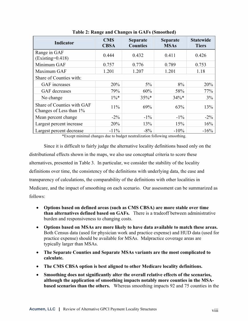
Table 2: Range and Changes in GAFs (Smoothed)

Indicator CMS CBSA

Separate Counties

Separate MSAs

Statewide Tiers

Range in GAF (Existing=0.418) 0.444 0.432 0.411 0.426

Minimum GAF 0.757 0.776 0.789 0.753 Maximum GAF 1.201 1.207 1.201 1.18 Share of Counties with: GAF increases 20% 5% 8% 20% GAF decreases 79% 60% 58% 77% No change 1%* 35%* 34%* 3%Share of Counties with GAF Changes of Less than 1%

11% 69% 63% 13%

Mean percent change -2% -1% -1% -2%Largest percent increase 20% 13% 15% 16%Largest percent decrease -11% -8% -10% -16%

*Except minimal changes due to budget neutralization following smoothing.

Since it is difficult to fairly judge the alternative locality definitions based only on the

distributional effects shown in the maps, we also use conceptual criteria to score these

alternatives, presented in Table 3. In particular, we consider the stability of the locality

definitions over time, the consistency of the definitions with underlying data, the ease and

transparency of calculations, the comparability of the definitions with other localities in

Medicare, and the impact of smoothing on each scenario. Our assessment can be summarized as

follows:

Options based on defined areas (such as CMS CBSA) are more stable over time than alternatives defined based on GAFs. There is a tradeoff between administrative burden and responsiveness to changing costs.

Options based on MSAs are more likely to have data available to match these areas. Both Census data (used for physician work and practice expense) and HUD data (used for practice expense) should be available for MSAs. Malpractice coverage areas are typically larger than MSAs.

The Separate Counties and Separate MSAs variants are the most complicated to calculate.

The CMS CBSA option is best aligned to other Medicare locality definitions.

Smoothing does not significantly alter the overall relative effects of the scenarios, although the application of smoothing impacts notably more counties in the MSA-based scenarios than the others. Whereas smoothing impacts 92 and 75 counties in the

Acumen, LLC | Review of Alternative GPCI Payment Locality Structures viii

CMS CBSA and Separate MSAs alternatives, respectively, it impacts only 33 and 54 counties in the Baseline and Separate Counties alternatives.

Table 3: Rank Ordering of Alternatives on Conceptual Criteria (Ties are scored at the average of the remaining rankings)

Criteria Baseline CMS CBSA

Separate Counties

Separate MSAs

Statewide Tiers

Stability over time 1 2 3 4 5

Alignment with underlying data 3 1 4 2 5

Ease of calculation 1 2 4 5 3

Comparability with other Medicare defn 4 1 4 4 4

Impact of Smoothing 1 4 2 3 N/A

Acumen, LLC | Review of Alternative GPCI Payment Locality Structures ix

Table of Contents

Summary......................................................................................................................................... i Introduction................................................................................................................................... 1

Report Organization.................................................................................................................... 3 Background ................................................................................................................................... 4

Data Sources ............................................................................................................................... 4 Smoothing Methodology ............................................................................................................ 7

0 ....................................................................... 11 Baseline: Fully Implemented 2009 GPCIs0.1 ............................................. 11 Approach to Defining Localities and Calculating GPCIs0.2 .......................................................... 12 Summary Statistics of Localities (Unsmoothed)0.3 .................................................................................... 14 Summary of Smoothing Impact

1 ..................................................................................................... 19 Scenario 1: CMS CBSA1.1 ............................................. 19 Approach to Defining Localities and Calculating GPCIs1.2 .......................................................... 20 Summary Statistics of Localities (Unsmoothed)1.3 .......................................................... 22 Summary of Impact on Counties (Unsmoothed)1.4 ............................................................... 27 Summary Statistics of Localities (Smoothed)1.5 .............................................................. 29 Summary of Impact on Counties (Smoothed)1.6 ..................................................................................................... 34 Impact of Smoothing

2 .............................. 38 Scenario 2: Separate High Cost Counties from Existing Localities2.1 ............................................. 38 Approach to Defining Localities and Calculating GPCIs2.2 .......................................................... 41 Summary Statistics of Localities (Unsmoothed)2.3 .......................................................... 42 Summary of Impact on Counties (Unsmoothed)2.4 ............................................................... 47 Summary Statistics of Localities (Smoothed)2.5 .............................................................. 49 Summary of Impact on Counties (Smoothed)2.6 ..................................................................................................... 53 Impact of Smoothing

3 ........................................................................................................................................ 56

Scenario 3: Separate High Cost Metropolitan Statistical Areas from statewide localities

3.1 ............................................. 56 Approach to Defining Localities and Calculating GPCIs3.2 .......................................................... 58 Summary Statistics of Localities (Unsmoothed)3.3 .......................................................... 60 Summary of Impact on Counties (Unsmoothed)3.4 ............................................................... 65 Summary Statistics of Localities (Smoothed)3.5 .............................................................. 66 Summary of Impact on Counties (Smoothed)3.6 ..................................................................................................... 71 Impact of Smoothing

4 ............................................................................................... 74 Scenario 4: Statewide Tiers4.1 ............................................. 74 Approach to Defining Localities and Calculating GPCIs4.2 .................................................................................. 75 Summary Statistics of Localities4.3 .................................................................................. 76 Summary of Impact on Counties

5 ............................................................................................. 81 Cross-Scenario Comparisons5.1 ................................................................................................. 81 Conceptual Differences5.2 ....................................................................... 83 Magnitude and Distribution of Changes5.3 ..................................................................................................... 86 Impact of Smoothing

Acumen, LLC | Review of Alternative GPCI Payment Locality Structures x

List of Tables and Figures

Table 1: Number of Localities under Each Scenario ..................................................................... iii Figure 1: GAF Percent Change: Baseline to CMS CBSA (Smoothed) ......................................... iv Figure 2: GAF Percent Change: Baseline to Separate Counties (Smoothed)................................. v Figure 3: GAF Percent Change: Baseline to Separate MSAs (Smoothed).................................... vi Figure 4: GAF Percent Change: Baseline to Statewide Tiers....................................................... vii Table 2: Range and Changes in GAFs (Smoothed) ..................................................................... viii Table 3: Rank Ordering of Alternatives on Conceptual Criteria ................................................... ix Stylized Example: A Demonstration of the Smoothing Methodology ........................................... 9 Table 0-1: Number of Localities per State, Baseline................................................................... 13 Table 0-2: Number of Counties per Locality, Baseline ............................................................... 13 Figure 0-1: GAF Percent Change: Baseline to Baseline (Smoothed)........................................... 15 Table 0-3: Summary of GAF Differences, Baseline to Baseline (Smoothed)............................. 16 Table 0-4: Number of Localities per State, Baseline to Baseline (Smoothed) ............................ 17 Table 0-5: Number of Counties per Locality, Baseline to Baseline (Smoothed) ........................ 17 Table 0-6: Counties Impacted by Smoothing of the Baseline ...................................................... 18 Table 1-1: Number of Localities per State, Baseline to CMS CBSA (Unsmoothed).................. 21 Table 1-2: Number of Counties per Locality, Baseline to CMS CBSA (Unsmoothed) .............. 21 Figure 1-1: GAF Percent Change: Baseline to CMS CBSA (Unsmoothed) ................................ 23 Table 1-3: Summary of GAF Differences, Baseline to CMS CBSA (Unsmoothed)................... 24 Table 1-4: Top 20 Increases, Baseline to CMS CBSA (Unsmoothed)........................................ 25 Table 1-5: Top 20 Decreases, Baseline to CMS CBSA (Unsmoothed) ...................................... 26 Table 1-6: Number of Localities per State, Baseline to CMS CBSA (Smoothed) ...................... 28 Table 1-7: Number of Counties per Locality, Baseline to CMS CBSA (Smoothed) .................. 28 Figure 1-2: GAF Percent Change: Baseline to CMS CBSA (Smoothed)..................................... 30 Table 1-8: Summary of GAF Differences, Baseline to CMS CBSA (Smoothed)....................... 31 Table 1-9: Top 20 Increases, Baseline to CMS CBSA (Smoothed) ............................................ 32 Table 1-10: Top 20 Decreases, Baseline to CMS CBSA (Smoothed)......................................... 33 Figure 1-3: Impact of Smoothing: CMS CBSA (Unsmoothed) to CMS CBSA (Smoothed)....... 34 Table 1-11: Counties Impacted by Smoothing under the CMS CBSA Scenario ........................ 35 Table 2-1: Example Case – Separate Counties Scenario Calculations Where a Gap Lower in the

GAF Ranking Does Not Yield Separate Localities .................................................. 40 Table 2-2: Number of Localities per State, Baseline to Separate Counties (Unsmoothed)......... 41 Table 2-3: Number of Counties per Locality, Baseline to Separate Counties (Unsmoothed)..... 42 Figure 2-1: GAF Percent Change: Baseline to Separate Counties (Unsmoothed) ....................... 43 Table 2-4: Summary of GAF Differences, Baseline to Separate Counties (Unsmoothed) ........ 44 Table 2-5: Top 20 Increases, Baseline to Separate Counties (Unsmoothed).............................. 45 Table 2-6: Top 20 Decreases, Baseline to Separate Counties (Unsmoothed) ............................ 46 Table 2-7: Number of Localities per State, Baseline to Separate Counties (Smoothed)............. 48 Table 2-8: Number of Counties per Locality, Baseline to Separate Counties (Smoothed) ......... 48 Table 2-9: Summary of GAF Differences, Baseline to Separate Counties (Smoothed)............. 49 Figure 2-2: GAF Percent Change: Baseline to Separate (Smoothed)........................................... 50 Table 2-10: Top 20 Increases, Baseline to Separate Counties (Smoothed) ................................ 51 Table 2-11: Top 20 Decreases, Baseline to Separate High Cost Counties (Smoothed) .............. 52

Acumen, LLC | Review of Alternative GPCI Payment Locality Structures xi

Acumen, LLC | Review of Alternative GPCI Payment Locality Structures xii

Figure 2-3: Impact of Smoothing: Separate Counties (Unsmoothed) to Separate Counties (Smoothed)................................................................................................................ 53

Table 2-12: Counties Impacted by Smoothing under the Separate Counties Scenario ................ 54 Table 3-1: Number of Localities per State, Baseline to Separate MSAs (Unsmoothed)............. 59 Table 3-2: Number of Counties per Locality, Baseline to Separate MSAs from Statewide

Localities (Unsmoothed)........................................................................................... 59 Figure 3-1: GAF Percent Change: Baseline to Separate MSAs (Unsmoothed) ........................... 61 Table 3-3: Summary of GAF Differences, Baseline to Separate MSAs (Unsmoothed) ............. 60 Table 3-4: Top 20 Increases, Baseline to Separate MSAs (Unsmoothed)................................... 63 Table 3-5: Top 20 Decreases, Baseline to Separate MSAs (Unsmoothed) ................................. 64 Table 3-6: Number of Localities per State, Baseline to Separate MSAs (Smoothed)................. 66 Table 3-7: Number of Counties per Locality, Baseline to Separate MSAs (Smoothed) ............. 66 Figure 3-2: GAF Percent Change: Baseline to Separate MSAs (Smoothed)................................ 67 Table 3-8: Summary of GAF Differences, Baseline to Separate MSAs (Smoothed).................. 68 Table 3-9: Top 20 Increases, Baseline to Separate MSAs (Smoothed)....................................... 69 Table 3-10: Top 20 Decreases, Baseline to Separate MSAs (Smoothed).................................... 70 Figure 3-3: Impact of Smoothing: Separate MSAs (Unsmoothed) to Separate MSAs (Smoothed)

................................................................................................................................... 71 Table 3-11: Counties Impacted by Smoothing under the Separate MSAs Scenario .................... 72 Table 4-1: Number of Localities per State, Baseline to Statewide Tiers.................................... 76 Table 4-2: Number of Counties per Locality, Baseline to Statewide Tiers ................................. 76 Table 4-3: Summary of GAF Differences, Baseline to Statewide Tiers...................................... 77 Figure 4-1: GAF Percent Change: Baseline to Statewide Tiers ................................................... 78 Table 4-4: Top 20 Increases, Baseline to Statewide Tiers........................................................... 79 Table 4-5: Top 20 Decreases, Baseline/Statewide Tiers ............................................................. 80 Table 5-1: Rank Ordering of Alternatives on Conceptual Criteria.............................................. 81 Table 5-2: Number of Localities under Each Scenario................................................................. 84 Table 5-3: Range and Changes in GAFs (Smoothed)................................................................... 84 Table 5-4: Impacts for Counties in MSAs Compared to Non-MSAs (Smoothed) ....................... 86 Table 5-5: Range and Changes in GAF ........................................................................................ 87 Table 5-6: Number of Counties Impacted by Smoothing............................................................. 87

INTRODUCTION

This report examines four alternatives to the current GPCI payment locality structure, based on geographic areas or costs.

As required by Section 1848(e) of the Social Security Act,

the Centers for Medicare and Medicaid Services (CMS) establish

geographic indices as part of the Resource-Based Relative Value

Scale (RBRVS) method for reimbursing physicians. Called the

Geographic Practice Cost Index or GPCI, geographic adjustment

was first implemented as part of the Medicare physician fee schedule

in 1992 and is required to be updated at least every three years. Like

the relative value units (RVUs), which are designed to provide

physicians with higher reimbursements for more costly services, the

GPCI is split into three components: the physician work GPCIW, the

practice expense GPCIPE and the malpractice insurance GPCIMP.

While the RVUs distinguish among services, the GPCI adjusts

payments for geographic variation in the costs of providing services.

By design, the GPCI balances the goal of accurately adjusting for

local cost differences with the goal of ensuring that physicians in

less expensive areas, especially rural areas, are not unduly

disadvantaged by downward adjustments in the GPCI.

The current GPCIs are calculated for 89 areas, down from

an original set of 210 payment areas prior to 1997. Since the

physician payment localities were last defined in 1996, there may

have been shifts in population and economic development. In some

localities, areas that were once rural may now be suburban or urban,

resulting in changes to the cost structure of rents and wages. CMS,

the General Accounting Office (GAO) and the Medicare Payment

Advisory Commission (MedPAC) have all published suggestions for

changes and/or improvements to the GPCI payment locality

structure.

Acumen, LLC | Review of Alternative GPCI Payment Locality Structures 1

Core Based Statistical Areas: CBSAs have at least one core urban area with a population of 10,000 or greater. CBSAs may also include adjacent areas having “a high degree of social and economic integration with the core as measured by commuting ties.”

Metropolitan Statistical Area: MSAs are core areas with a population of 50,000 or greater, plus adjoining areas that have “a high degree of social and economic integration with the core as measured by commuting ties.”

Micropolitan Statistical Area: Micropolitans are core areas with at least one urban area having a population of 10,000 or greater but which also have a total population of less than 50,000, plus adjoining areas that have “a high degree of social and economic integration with the core as measured by commuting ties.”

Metropolitan Division: OMB added Metropolitan Divisions in 2003, in order to differentiate smaller groupings of counties within MSAs that have a population of 2.5 million or more. The concept of Metropolitan Divisions replaces that of Primary Metropolitan Statistical Areas (PMSAs).

Source: Office of Management and Budget. November 2007. Update of Statistical Area Definitions and Guidance on Their Uses. OMB Bulletin No. 08 – 01.

In this report, we consider potential scenarios for redefining the GPCI locality areas, with

analysis that compares these alternative locality configurations to the Fully Implemented

CY2009 Payment Structure (the Baseline) now used to calculate GPCI reimbursements. The

alternative scenarios distinguish locality payment structures based on two primary

characteristics: (1) the base geographic unit used to structure the locality payment option (i.e.,

counties or Metropolitan Statistical Areas (MSAs)) and (2) whether the payment structure option

uses costs to define the areas or uses an external geographical definition. The four scenarios are:

1. CMS CBSA – Based on geographic areas defined by OMB, the CMS CBSA option uses Metropolitan Statistical Areas (MSAs) and Metropolitan Divisions (MDs) to form localities in each state. Counties not included in MSAs are combined into non-MSA rest of state areas. This option most closely matches locality definitions used in other aspects of the Medicare program.

2. Separate High Cost Counties From Existing Localities – Starting with the existing GPCI localities, this scenario iteratively removes high cost counties.

3. Separate High Cost MSAs from Statewide Localities – Conceptually similar to the second alternative, the third alternative scenatio starts with statewide localities and iteratively removes high cost MSAs.

4. Statewide Tiers – The fourth alternative we consider groups counties into tiers within states based on their costs. This option was designated by CMS as “Option 3” in its Proposed Rule (72 FR 38141) of July 12, 2007.

Moreover, for three of these four locality definitions, we analyze the scenario with and without

the implementation of a smoothing methodology suggested by MedPAC, essentially leading to


seven alternative locality configurations in total.5 Smoothing is designed to limit the maximum

difference in GAFs between any two adjacent counties to ten percent.

Report Organization

The report is organized as follows. The background section reviews the data used in the

development of the GPCIs and, by extension, in the definition of the cost-based locality

scenarios. The background also presents the smoothing methodology applied to each scenario.

We then present the Baseline (existing 2009 locality definitions) and each of the alternative

scenarios. For each option we provide an overview of the definition of the localities. We also

present summary statistics for the GAF values under each definition and consider the county-

level impacts of changing from the existing localities to this alternative, first without smoothing

and then with smoothing when applied. Lastly, for scenarios with smoothing, we present the

impact of the smoothing methodology relative to the unsmoothed scenario. The final chapter

compares the alternatives, offering pros and cons for the different options. Two appendices are

not included in the report, but may be found at the following link:

http://www.cms.hhs.gov/PhysicianFeeSched/downloads/GPCIappendices.zip. Appendix A

contains tables listing all counties showing GAF increases of greater than five percent in any

scenario. Finally, both unsmoothed and smoothed GPCI locality values generated under each

option are included in Appendix B.

5 This report does not include a Statewide Tiers alternative with smoothing because the tiers are constructed according to county GAFs rather than according to county’s proximity to and economic relation with metropolitan areas. Whereas the other localities are at least partially defined using geographic location, the Statewide Tiers option defines localities according to GAF, by state.


http://www.cms.hhs.gov/PhysicianFeeSched/downloads/GPCIappendices.zip

BACKGROUND

The scenarios presented in this paper are all based on a common set of “county-level

GPCI” values. These values were developed following the methodology used for the 2009 GPCI

update, except that all counties were treated as individual localities. (See Medicare Physician

Fee Schedule Geographic Practice Cost Index (GPCI) Fifth Update, Final Report, November

2007.) In addition, the smoothing methodology we employ is the same across the different

scenarios. As background to the analyses that follow, this section reviews the data sources,

including important caveats in interpreting the data. It then describes the smoothing

methodology.

Data Sources

Although each of the scenarios we present are based on a data set of “county-level GPCI”

values, the underlying data do not typically represent physician practice costs in individual

counties. That is, the data are not county-level information, because the data sources were

chosen to reflect the existing 89 payment localities, rather than individual counties. In practical

terms, the four major data sources used in the development of the GPCIs are provided at

different geographic levels, usually representing more than a single county. As a result, the

county-level values are not necessarily the same as the estimates one would get if the data

collection were designed to reflect actual county costs. The specific sources and geographic

units are:

Source Data Used GPCI Geographic Unit

Decennial Census

Earnings and employment information for professional

occupations and non-physician practice employees

Physician Work Practice

Expense Census Work Area

HUD Median rent for 2-bedroom apartments

Practice Expense

MSA, HUD FMR Areas, County or

New England Towns


Source Data Used GPCI Geographic Unit

Insurance Carrier Rate Filings

Malpractice/professional liability insurance premiums Malpractice Insurer rating

territories

CMS Relative value units (RVUs) All County

The Physician Work and Practice Expense GPCIs both rely on data on earnings and the

number of workers drawn from the 2000 Census. The Census data are provided by “Census

work areas.” The Census work areas generally represent the smallest reliable units that align

with the Medicare payment locality definitions; the data were provided by Census through a

special tabulation. There are 545 work areas including the 233 counties that comprise the 19

consolidated metropolitan statistical areas (CMSAs),6 262 metropolitan statistical areas (MSAs)

or New England County metropolitan areas (NECMAs), and 50 rural “balance of state” areas.

For work areas that encompass multiple counties, all counties in the work area were assigned the

same occupational data. Census suppresses data in areas with too few observations in a given

occupation. For example, Census suppressed data on pharmacists in 28 work areas. All

combined, occupation-by-work-area results were suppressed in 74 cases, including 55 in Puerto

Rico.

The rent data collected by the U.S. Department of Housing and Urban Development

(HUD) are calculated for HUD areas. The HUD areas are commonly metropolitan statistical

areas, although in some cases HUD creates its own area definitions. In New England, the areas

are defined based on sets of towns, largely based on defined New England City and Town Areas

(NECTA). Outside of MSAs and NECTAs, HUD presents rent data for non-metropolitan areas

at the county level. In the MSAs and NECTAs, the rent data incorporates information from

ongoing housing surveys. In the non-metropolitan counties, the HUD data merely update

information from the 2000 Census.

The largest geographical boundaries are typically those used as inputs for the Malpractice

GPCI, where the GPCIs rely on insurance carrier rate filings, and therefore use the rating

territories defined by insurers. Within a given state, different insurers will have different rate 6 CMSAs are no longer used in OMB statistical definitions. They represent the MSAs that now include Metropolitan Divisions. Using current terminology, both the 2000 CMSAs and MSAs are now considered MSAs.


boundaries, and the sizes of these boundaries differ by carrier and state. In some states, specific

counties or cities may have separate rate territories, but the territories are more often regional.

For example, in California, the three insurers included in the malpractice data had nine, six and

five territories each, although the insurer with five territories had switched which counties were

in which territory.

Finally, the GPCI data are all weighted by RVUs for the purpose of developing national

average values as well as aggregating counties within localities. Since RVUs are based on CMS’

own claims data, these data are available at fine levels of detail (and represent the universe of

data rather than a sample). The RVU information is provided by CMS at the county level.

Caveats

There are three caveats to note as background for these calculations. First, we had to

adjust some data to account for missing RVUs. Second, we do not have underlying data for

three territories: American Samoa, the Northern Mariana Islands and Guam. Third, the data has

not been budget neutralized for updates made to the 2009 GPCIs. We briefly review each of

these issues below.

There are two groups of counties or regions that are problematic when using the county-

level GPCI values. First, there are 87 counties that had no RVUs in the 2005 RVU file used to

create the updated GPCIs. An additional 12 counties had no physician work RVUs, but did have

RVUs for practice expense or malpractice insurance. RVUs are used at multiple stages in the

GPCI calculation to create weighted averages, including national averages to norm the GPCIs

around one. If a county’s RVUs are missing at any step in the analysis, the county-level GPCI

value for that county is missing. This is not a problem under the existing locality definitions,

because the localities are predefined, and the GPCI information from the remaining counties in

the locality then determines the locality GPCI. In some of the alternative scenarios, however,

county-level GPCI values (summarized as the Geographic Adjustment Factor or GAF) are used

to define localities.

To ensure that localities were defined for every county under every scenario, we re-

created the county-level GPCI values. We addressed the issue of missing RVUs by setting the

RVU values for those counties to very near zero. This prevents the generation of missing values

for the county-level GPCIs without affecting the locality level GPCIs as previously calculated.


The second problem is more difficult to resolve. Among the territories, Census data

were only available for Puerto Rico, and HUD data were available only for Puerto Rico and the

Virgin Islands. No malpractice premium data were available for any of the territories. In the

existing GPCIs, Puerto Rico and Virgin Islands are separate localities. For Puerto Rico, the

updated GPCIs use the appropriate Census and HUD data and simply keep the previous GPCI

value for the malpractice premium. For the Virgin Islands, the updated GPCIs use the available

HUD data and set all other values to 1.0, in the absence of other data. This leaves American

Samoa, Guam and the Northern Mariana Islands as the only territories without any underlying

data. Therefore, following the method used in the existing GPCIs, we assigned these territories

the same GPCI values as non-metropolitan Hawaii in all alternative scenarios.

Finally, we note that the values calculated here represent non-budget neutralized GAFs

and GPCIs, in the sense that they do not include the budget neutrality factors for the 2009 update

of the GPCIs. These changes were minimal. In any case, the budget neutralization primarily

addresses changes in the distribution of the RVUs over time. If more resource use growth has

occurred in high cost areas than in low cost areas, budget neutralization is required to hold

updated GPCIs constant when weighted by RVUs. More importantly, the adjustments required

are identical across all of the locality definitions, because the RVU weights are already

accounted for in the initial county-level data set.

Although the calculations do not account for the budget neutralization to the 2009 value,

all of the alternatives are budget neutral to the baseline. That is, the net RVU-weighted change is

identically equal to zero for all scenarios.

Smoothing Methodology

All of the alternative locality configuration scenarios in this report, other than the

Statewide Tiers option, include smoothing to eliminate large differences (or “cliffs”) between

adjacent counties. For all cases, we employ the smoothing methodology recommended by

MedPAC for the hospital wage index in their June 2007 report to Congress.7 MedPAC refers to

their smoothing approach as “step smoothing,” which is done in four steps:

1. Compare all counties to each adjacent county 7 See “Additional technical information on constructing a compensation index from BLS data,” in the appendix to Chapter 6 of the Report to the Congress: Promoting Greater Efficiency in Medicare (June 2007).


2. Find the greatest differences between pairs of adjacent counties

3. If the difference between adjacent counties exceeds ten percent (or another threshold), increase the lower index to 90 percent of the greater index in the pair, and

4. Repeat as needed.

At the end of this process, the smoothed values need to be budget neutralized to account for the

increases applied in Step 3 (that is, to keep them budget neutral relative to the existing GPCIs).

We have confirmed with MedPAC analysts that this smoothing is conducted nationwide.8

Therefore, the smoothing eliminates large differences between adjacent counties even if the

counties are in different states. Because the smoothing crosses state boundaries, the budget

neutralization is also nationwide. Although the impacts will be very small, this approach does

mean that states without any cliffs will help pay for the increased GAFs for counties subject to

the smoothing.

The following example details the smoothing approach. Imagine there were only two

states with eight counties, as shown below. To implement the smoothing, we compare the GAF

value for each county (shown in the figure) to the values for all adjacent counties, as listed below

the figure. For each row, we identify the maximum GAF. If this maximum is greater than 110

percent of that county’s GAF, the county is assigned a GAF equal to 90 percent of that maximum

GAF. Among the counties shown in the figure, only County D and County G have adjacent

counties with GAFs greater than 110 percent. In this example, County D’s GAF is smoothed to

90% of County A and County G’s GAF is set to 90 percent of County E. These new values are

shown for Round 1 of the Smoothing. However, County D’s new GAF is now more than 110

percent of County H, so in the second round, the GAF for County H also increases.

8 Personal communication with David Glass and Jeff Stensland, 4/22/08.


Stylized Example: A Demonstration of the Smoothing Methodology

Notably, for the case of counties not belonging to single-county localities, smoothing

effectively results in the creation of an additional locality because it raises the GAF of only those

counties with cliffs of ten percent or greater. When smoothed counties are the only county in


their locality, as sometimes occurs, no additional locality is created. However, as is most often

the case, when a county belongs to a locality that also contains other counties, smoothing has the

effect of pulling that county out of the old locality and creating a new, single-county locality. In

these multi-county locality cases, the GAF of the old locality will be unaffected by the change,

with the exception of the budget neutralization applied to all counties, as explained below.

Finally, because Counties D, G and H have higher GAFs after smoothing, the last step is

to budget neutralize all values so that they reflect the same total weighted GAF value as prior to

the smoothing process. To do this, we calculate the sum of the pre-smoothed RVU-weighted

GAFs as a share of the sum of the smoothed RVU-weighted GAFs, or:

993.684.862.8

)*(

)*(

,

,

H

Accsmoothedc

H

Accunsmoothedc

RVUGAF

RVUGAF.

In other words, in this example, all of the GAFs (i.e. all of the underlying GPCIs) need to be

reduced by 0.7 percent (1-0.993) to account for the increases made in the smoothing process.

This example is extreme – in practice, the final reductions are less than 0.1 percent applied for all

counties.


0 BASELINE: FULLY IMPLEMENTED 2009 GPCIS

Unsmoothed Baseline: The “Baseline” locality definitions are the existing 89 localities

currently used by CMS to calculate GPCIs.

0.1 Approach to Defining Localities and Calculating GPCIs

The current GPCIs are calculated for 89 areas defined by CMS, as shown on Figure 0-1.

The 89 locality structure was established to rationalize the original system of 210 localities

established by the Part B carrier with the goals of simplifying payment areas and reducing

differences between payment areas. The 1996 locality definitions kept 22 pre-existing statewide

localities. For the remaining 28 states, the new localities were calculated by grouping localities

where the GAFs were not sufficiently different from the rest of the state to meet the threshold for

a separate locality. In Massachusetts, Missouri and Pennsylvania, localities had to be redefined

to eliminate non-contiguous subcounty areas. (The use of subcounty level localities was viewed

as overly burdensome, since all of the underlying data had to be mapped down to zip codes and

city boundaries.)

Geographic Units:

Blend of states, metropolitan areas, individual counties, and “rest of state” areas.

Calculations:

As defined-area localities, the baseline GPCIs are RVU-weighted averages of the county

values derived from the GPCI input data. For example, if we denote the county-level values of

the inputs for the Physician Work GPCI as GPCIPW,c then for each locality L, the existing

locality GPCIs are calculated as:

(0.1)

C

ccPW

C

ccPWcPW

RVU

RVUGPCI

1,

1,,

L PW,

)*(GPCI ,

where the value of C depends on the number of counties in the locality. For single county

localities, C is equal to 1. For entire state localities, C is equal to the number of counties in the


state. A parallel calculation is done to yield the Practice Expense GPCI for each locality L,

GPCIPE,L, and the Malpractice Premium GPCI for each locality, GPCIMP,L.

For comparison purposes, the three GPCIs for any given locality are summarized using

the Geographic Adjustment Factor (GAF), calculated for locality L as:

(0.2) 03865.0*43669.0*52466.0* GPCIGPCIGPCIGAF ,,, LMPLPELPWL .

0.2 Summary Statistics of Localities (Unsmoothed)

To summarize the findings for each alternative, we review summary statistics by locality.

In this section, we consider the summary statistics for the Baseline, which will serve as the basis

of comparison for each alternative. The core measures we consider for localities include:

Number of localities: 89

Highest GAF: 1.208 (San Mateo, CA)

Lowest GAF: 0.790(Puerto Rico, PR)

Range in GAF (Highest – Lowest): 0.418

As shown in Table 0-1, another way of summarizing the alternative scenarios is to

consider the number of localities generated in each state. Under the Baseline, the smallest

number of localities per state is 1 – for the statewide localities – and the highest is 9, found in

California. There are as many as 245 counties in a given locality (Rest of Texas) and as few as

one county.


Table 0-1: Number of Localities per State, Baseline

State Baseline Localities State Baseline

Localities

Alabama 1 Nebraska 1 Alaska 1 Nevada 1 Arizona 1 New Hampshire 1 Arkansas 1 New Jersey 2 California 9 New Mexico 1 Colorado 1 New York 5 Connecticut 1 North Carolina 1 Delaware 1 North Dakota 1 District of Columbia 1 Ohio 1 Florida 3 Oklahoma 1 Georgia 2 Oregon 2 Hawaii 1 Pennsylvania 2 Idaho 1 Puerto Rico 1 Illinois 4 Rhode Island 1 Indiana 1 South Carolina 1 Iowa 1 South Dakota 1 Kansas 1 Tennessee 1 Kentucky 1 Texas 8 Louisiana 2 Utah 1 Maine 2 Vermont 1 Maryland 2 Virgin Islands 1 Massachusetts 2 Virginia 1 Michigan 2 Washington 2 Minnesota 1 West Virginia 1 Mississippi 1 Wisconsin 1 Missouri 3 Wyoming 1 Montana 1 Total 89

Table 0-2: Number of Counties per Locality, Baseline

Baseline Mean 36 Median 12.5 Standard Deviation 44 Maximum 247 Minimum 1 Range 246



0.3 Summary of Smoothing Impact

Baseline Smoothed: The “Baseline Smoothed” locality scenario uses the existing

baseline GPCIs but applies the smoothing methodology to eliminate differences exceeding 10

percent between adjacent counties. We provide this option to highlight the impact of the

smoothing from the impact of the alternative locality definitions.

Smoothing the Baseline scenario does not change the highest and lowest GAF values and

their respective counties. However, because smoothing effectively pulls out high-GAF counties

from their former localities when they reside in multi-county localities, the summary statistics for

the number of localities per state and counties per locality generally decrease.

Number of GAF decreases: 0

Number of GAF increases: 30

Number with no change*: 3198

Number with less than 1% change: 3206

Mean percentage change: -0.0%**

Largest percent increase: 7.1% (Santa Cruz, California)

Largest percent decrease: -0.1% (3195 counties) *Counties that only experienced a change due to the budget neutrality from smoothing were excluded from the GAF decreases and considered as “no change.”

**Value represents a negative change less than 0.05%.

The smoothing primarily benefits counties currently included in “Rest of State” localities

in California, Pennsylvania and the Virginia/Maryland area, as well as a handful of counties

outside Chicago. Overall, 30 counties benefit from smoothing – these are listed in Table 0-6 and

depicted in Figure 0-1. Three additional counties had increases due to smoothing but too

minimal to offset the (also minimal) decrease due to budget neutralization. All other counties are

only affected by the very minor decline of 0.1 percent, the impact of budget neutralization

applied to all counties following the smoothing. As a result we have grouped those counties

(along with the three minimally decreasing smoothed counties) that only experienced a change

due to budget neutrality from smoothing as “no change” since there is no direct effect on these

counties.

Figure 0-1: GAF Percent Change: Baseline to Baseline (Smoothed)


Table 0-3: Summary of GAF Differences, Baseline to Baseline (Smoothed)

GAF Differences Index Value Difference

Percent Difference

Mean 0.000 -0.0%** RVU Weighted Mean 0.000 0.0%* Median 0.000 -0.1% Minimum -0.001 -0.1% 25th Percentile 0.000 -0.1% 75th Percentile 0.000 -0.1% Maximum 0.072 7.1% Range 0.072 7.1% Std. Dev 0.003 0.3% * Value represents a positive change less than 0.05%. **Value represents a negative change less than 0.05%.


Table 0-4: Number of Localities per State, Baseline to Baseline (Smoothed)

State Baseline Baseline Smoothed State Baseline Baseline

Smoothed Alabama 1 1 Nebraska 1 1 Alaska 1 1 Nevada 1 1 Arizona 1 1 New Hampshire 1 2 Arkansas 1 1 New Jersey 2 2 California 9 18 New Mexico 1 1 Colorado 1 1 New York 5 6 Connecticut 1 1 North Carolina 1 1 Delaware 1 1 North Dakota 1 1 District of Columbia 1 1 Ohio 1 1 Florida 3 3 Oklahoma 1 1 Georgia 2 2 Oregon 2 2 Hawaii 1 1 Pennsylvania 2 8 Idaho 1 4 Puerto Rico 1 1 Illinois 4 9 Rhode Island 1 1 Indiana 1 2 South Carolina 1 1 Iowa 1 1 South Dakota 1 1 Kansas 1 1 Tennessee 1 1 Kentucky 1 1 Texas 8 8 Louisiana 2 2 Utah 1 1 Maine 2 2 Vermont 1 1 Maryland 2 5 Virgin Islands 1 1 Massachusetts 2 2 Virginia 1 3 Michigan 2 2 Washington 2 2 Minnesota 1 1 West Virginia 1 1 Mississippi 1 1 Wisconsin 1 2 Missouri 3 3 Wyoming 1 1 Montana 1 1 Total 89 122*

*Including 33 counties affected by Smoothing.

Table 0-5: Number of Counties per Locality, Baseline to Baseline (Smoothed)

Baseline Baseline Smoothed

Mean 36 26 Median 12.5 4 Standard Deviation 44 41 Maximum 247 247 Minimum 1 1 Range 246 246



Table 0-6: Counties Impacted by Smoothing of the Baseline Baseline GAF

County State Unsmoothed Smoothed and

Budget Neutralized Value

Difference Percent

Difference Santa Cruz CA 1.015 1.087 0.072 7.1% Loudoun VA 0.955 1.012 0.057 6.0% Prince William VA 0.955 1.012 0.057 6.0% Monroe PA 0.969 1.024 0.055 5.7% Northampton PA 0.969 1.024 0.055 5.7% Pike PA 0.969 1.024 0.055 5.7% Lake IN 0.944 0.978 0.034 3.6% McHenry IL 0.945 0.978 0.033 3.5% Hillsborough NH 0.989 1.023 0.034 3.4% Calvert MD 0.987 1.012 0.025 2.5% Charles MD 0.987 1.012 0.025 2.5% Frederick MD 0.987 1.012 0.025 2.5% Kenosha WI 0.939 0.959 0.02 2.1% Merced CA 1.015 1.036 0.021 2.1% San Benito CA 1.015 1.036 0.021 2.1% Stanislaus CA 1.015 1.036 0.021 2.1% DeKalb IL 0.945 0.959 0.014 1.4% Grundy IL 0.945 0.959 0.014 1.4% Kankakee IL 0.945 0.959 0.014 1.4% Kendall IL 0.945 0.959 0.014 1.4% Orange NY 1.037 1.049 0.011 1.1% Putnam NY 1.037 1.049 0.011 1.1% Sacramento CA 1.015 1.021 0.006 0.6% San Joaquin CA 1.015 1.021 0.006 0.6% Riverside CA 1.015 1.018 0.003 0.3% San Bernardino CA 1.015 1.018 0.003 0.3% San Diego CA 1.015 1.018 0.003 0.3% Berks PA 0.969 0.969 0.000 0.0%* Lancaster PA 0.969 0.969 0.000 0.0%* Lehigh PA 0.969 0.969 0.000 0.0%* Cassia ID 0.917 0.917 0.000 -0.0%** Owyhee ID 0.917 0.917 0.000 -0.0%** Twin Falls ID 0.917 0.917 0.000 -0.0%**

*Value represents a positive change less than 0.05%. **Value represents a negative change less than 0.05%.

1 SCENARIO 1: CMS CBSA

CMS CBSA: The CMS CBSA localities are Metropolitan Statistical Areas (MSAs), or

Metropolitan Divisions (MDs) within MSAs, and “non-MSA” rest of state areas.


The first scenario, called the CMS CBSA option, follows the approach CMS uses to

develop geographic payment adjustments for the End Stage Renal Disease (ESRD), the skilled

nursing facility ambulatory surgical center (SNF ASC), and home health benefits. The localities

are a variant of the Core Base Statistical Areas (CBSAs) established by the Office of Budget and

Management. CBSAs include three types of defined areas: Metropolitan Statistical Areas

(MSAs), subsets of MSAs known as Metropolitan Divisions (MDs) and Micropolitan Statistical

Areas. The CMS CBSA option uses MSAs and, within MSAs the MDs to distinguish urban

areas from rural areas but does not use Micropolitan Areas. All non-MSA counties, including

Micropolitan Areas, are grouped together in “non-MSA” rest of state areas.

Geographic Units:

MSAs, MSA MDs and non-MSAs. There are no statewide localities in this scenario.

Calculations:

The CMS CBSA localities are similar to the Baseline localities in that they are defined-

area localities. The MSAs and MSA MDs were identified using the January 11, 2008 State and

County to CBSA Crosswalk provided by CMS. All counties in a defined MSA or MSA-MD are

combined into a locality, taking the RVU-weighted average value for the GPCIs for the counties

in the locality. All counties not comprising MSAs within a state are included in the State’s non-

MSA locality. This approach is identical to that for the Baseline, using redefined localities.

For example, if we denote the county-level values of the inputs for the Physician Work GPCI as

GPCIPW,c then for each MSA, MSA-MD or non-MSA area, the CMS CBSA locality GPCIs are

calculated as:


(1.1)

C

ccPW

C

ccPWcPW

PW, M

RVU

RVUGPCI

1,

1,, )*(

GPCI ,

where the value of C depends on the number of counties in the MSA, MSA-MD or non-MSA

area, denoted by M. A parallel calculation is done to yield the Practice Expense GPCI for each

area M, GPCIPE,M, and the Malpractice Premium GPCI for each locality, GPCIMP,M. To

summarize these GPCIs, GAFs are calculated using the same formula as in (0.1).


As with the Baseline, we summarize the findings for the CMS CBSA alternative by first

examining the summary statistics for the locality. This approach yields a much larger number of

localities, compared to the Baseline:


Highest GAF: 1.201 (San Fran-San Mateo-Redwood City, CA)

Lowest GAF: 0.757 (Aguadilla-Isabela-San Sebastián, PR)

Range in GAF: 0.444


Table 1-1: Number of Localities per State, Baseline to CMS CBSA (Unsmoothed)

State Baseline CBSA State Baseline CBSA

Alabama 1 12 Nebraska 1 4 Alaska 1 3 Nevada 1 4 Arizona 1 7 New Hampshire 1 3 Arkansas 1 8 New Jersey 2 7 California 9 28 New Mexico 1 5 Colorado 1 8 New York 5 14 Connecticut 1 5 North Carolina 1 15 Delaware 1 3 North Dakota 1 4 District of Columbia 1 1 Ohio 1 13 Florida 3 23 Oklahoma 1 4 Georgia 2 15 Oregon 2 7 Hawaii 1 2 Pennsylvania 2 15 Idaho 1 6 Puerto Rico 1 9 Illinois 4 11 Rhode Island 1 1 Indiana 1 15 South Carolina 1 9 Iowa 1 9 South Dakota 1 3 Kansas 1 4 Tennessee 1 11 Kentucky 1 6 Texas 8 26 Louisiana 2 9 Utah 1 6 Maine 2 4 Vermont 1 2 Maryland 2 6 Virgin Islands 1 1 Massachusetts 2 8 Virginia 1 10 Michigan 2 16 Washington 2 12 Minnesota 1 5 West Virginia 1 7 Mississippi 1 5 Wisconsin 1 13 Missouri 3 8 Wyoming 1 3 Montana 1 4 Total 89 439

Table 1-2: Number of Counties per Locality,

Baseline to CMS CBSA (Unsmoothed) Baseline CMS CBSA Mean 36 7 Median 12.5 2 Standard Deviation 44 17 Maximum 247 177 Minimum 1 1 Range 246 176



1.3 Summary of Impact on Counties (Unsmoothed)

We compare each of the alternative scenarios to the Baseline to understand its impact on

individual counties. For each scenario, we determine the number of counties experiencing a

decrease, increase or no change in the GAF, as well as the magnitude of these changes. These

findings are depicted graphically in the map and are also summarized below and in Table 1-3.

The map in Figure 1-1 shows the percentage change in GAFs between the Baseline and

the CMS CBSA alternative. Counties that have a GAF under this alternative that is more than

1% lower than they have under the existing localities are shaded blue, with the deeper blue

indicating a larger percentage decline. Counties with increases greater than 1% are shown in

orange, with a deeper shade indicating a larger increase.

Number of GAF decreases: 2,582


Number with no change: 13


Mean percentage change: -2.0%

Largest percent increase: 20.0% (Jefferson County, West Virginia)

Largest percent decrease: -15.6% (Monroe County, Florida)

Figure 1-1: GAF Percent Change: Baseline to CMS CBSA (Unsmoothed)


Table 1-3: Summary of GAF Differences, Baseline to CMS CBSA (Unsmoothed)


Percent Difference

Mean -0.019 -2.0% RVU Weighted Mean 0.000 0.0%* Median -0.028 -3.1% Minimum -0.174 -15.6% 25th Percentile -0.035 -3.7% 75th Percentile -0.006 -0.7% Maximum 0.185 20.0% Range 0.359 35.5% Std. Dev 0.031 3.3% * Value represents a positive change less than 0.05%.

Compared to Baseline, the CMS CBSA option primarily benefits metropolitan areas in

statewide localities, as well as some more urbanized areas within existing “Rest of State”

localities. Most counties would have a decrease in their GAFs in shifting to the CMS CBSA

alternative, with an (unweighted) average decline of about two percent. The median county

would experience a decline of 3.1 percent; just less than one-fourth of counties experience an

increase. Table 1-4 and Table 1-5 report the counties experiencing the largest changes.


Table 1-4: Top 20 Increases, Baseline to CMS CBSA (Unsmoothed)

GAF County State Baseline Locality CMS CBSA Locality

Baseline CMS CBSA

Value Difference

Percent Difference

Jefferson WV West Virginia Washington-Arlington-Alexandria, DC-VA 0.927 1.112 0.185 20.0% Clarke VA Virginia Washington-Arlington-Alexandria, DC-VA 0.955 1.112 0.157 16.4% Fauquier VA Virginia Washington-Arlington-Alexandria, DC-VA 0.955 1.112 0.157 16.4% Loudoun VA Virginia Washington-Arlington-Alexandria, DC-VA 0.955 1.112 0.157 16.4% Prince William VA Virginia Washington-Arlington-Alexandria, DC-VA 0.955 1.112 0.157 16.4% Spotsylvania VA Virginia Washington-Arlington-Alexandria, DC-VA 0.955 1.112 0.157 16.4% Stafford VA Virginia Washington-Arlington-Alexandria, DC-VA 0.955 1.112 0.157 16.4% Warren VA Virginia Washington-Arlington-Alexandria, DC-VA 0.955 1.112 0.157 16.4% Fredericksburg city VA Virginia Washington-Arlington-Alexandria, DC-VA 0.955 1.112 0.157 16.4% Manassas city VA Virginia Washington-Arlington-Alexandria, DC-VA 0.955 1.112 0.157 16.4% Manassas Park city VA Virginia Washington-Arlington-Alexandria, DC-VA 0.955 1.112 0.157 16.4% Pike PA Rest of Pennsylvania Newark-Union, NJ-PA 0.969 1.125 0.156 16.1% DeKalb IL Rest of Illinois Chicago-Naperville-Joliet, IL 0.945 1.079 0.134 14.2% Grundy IL Rest of Illinois Chicago-Naperville-Joliet, IL 0.945 1.079 0.134 14.2% Kendall IL Rest of Illinois Chicago-Naperville-Joliet, IL 0.945 1.079 0.134 14.2% McHenry IL Rest of Illinois Chicago-Naperville-Joliet, IL 0.945 1.079 0.134 14.2% San Benito CA Rest of California San Jose-Sunnyvale-Santa Clara, CA 1.015 1.149 0.134 13.2% Kenosha WI Wisconsin Lake County-Kenosha County, IL-WI 0.939 1.058 0.119 12.6% Calvert MD Rest of Maryland Washington-Arlington-Alexandria, DC-VA 0.987 1.112 0.125 12.6% Charles MD Rest of Maryland Washington-Arlington-Alexandria, DC-VA 0.987 1.112 0.125 12.6%


Table 1-5: Top 20 Decreases, Baseline to CMS CBSA (Unsmoothed)

GAF County State Baseline Locality CMS CBSA Locality

Baseline CMS CBSA

Value Difference

Percent Difference

Monroe FL Miami, FL Florida (FL), non-MSA 1.117 0.943 -0.174 -15.6% Sullivan NY Poughkpsie/ N NYC Suburbs, NY New York (NY), non-MSA 1.037 0.925 -0.112 -10.8% Greene NY Poughkpsie/ N NYC Suburbs, NY New York (NY), non-MSA 1.037 0.925 -0.112 -10.8% Delaware NY Poughkpsie/ N NYC Suburbs, NY New York (NY), non-MSA 1.037 0.925 -0.112 -10.8% Columbia NY Poughkpsie/ N NYC Suburbs, NY New York (NY), non-MSA 1.037 0.925 -0.112 -10.8% Warren NJ Northern NJ Allentown-Bethlehem-Easton, PA-NJ 1.138 1.025 -0.114 -10.0% Washington IL East St. Louis, IL Illinois (IL), non-MSA 0.991 0.904 -0.087 -8.8% Randolph IL East St. Louis, IL Illinois (IL), non-MSA 0.991 0.904 -0.087 -8.8% Montgomery IL East St. Louis, IL Illinois (IL), non-MSA 0.991 0.904 -0.087 -8.8% Allegany MD Rest of Maryland Cumberland, MD-WV 0.987 0.906 -0.080 -8.2% Yellow Medicine MN Minnesota Minnesota (MN), non-MSA 0.962 0.887 -0.075 -7.8% Winona MN Minnesota Minnesota (MN), non-MSA 0.962 0.887 -0.075 -7.8% Wilkin MN Minnesota Minnesota (MN), non-MSA 0.962 0.887 -0.075 -7.8% Watonwan MN Minnesota Minnesota (MN), non-MSA 0.962 0.887 -0.075 -7.8% Waseca MN Minnesota Minnesota (MN), non-MSA 0.962 0.887 -0.075 -7.8% Wadena MN Minnesota Minnesota (MN), non-MSA 0.962 0.887 -0.075 -7.8% Traverse MN Minnesota Minnesota (MN), non-MSA 0.962 0.887 -0.075 -7.8% Todd MN Minnesota Minnesota (MN), non-MSA 0.962 0.887 -0.075 -7.8% Swift MN Minnesota Minnesota (MN), non-MSA 0.962 0.887 -0.075 -7.8% Stevens MN Minnesota Minnesota (MN), non-MSA 0.962 0.887 -0.075 -7.8%


1.4 Summary Statistics of Localities (Smoothed)

As with the unsmoothed CMS CBSA, we summarize the findings for the smoothed

alternative by first examining the summary statistics for the localities. This approach yields a

much larger number of localities compared to the Baseline:

Number of localities: 523*


Lowest GAF: 0.757 (Aguadilla-Isabela-San Sebastián, PR)

Range in GAF: 0.444 *Including 84 counties affected by smoothing that were not previously a single-county locality.


Table 1-6: Number of Localities per State, Baseline to CMS CBSA (Smoothed)

State Baseline CBSA Smoothed State Baseline CBSA

Smoothed Alabama 1 15 Nebraska 1 2 Alaska 1 9 Nevada 1 4 Arizona 1 7 New Hampshire 1 3 Arkansas 1 3 New Jersey 2 9 California 9 31 New Mexico 1 9 Colorado 1 8 New York 5 15 Connecticut 1 5 North Carolina 1 16 Delaware 1 3 North Dakota 1 2 District of Columbia 1 1 Ohio 1 15 Florida 3 27 Oklahoma 1 4 Georgia 2 19 Oregon 2 9 Hawaii 1 2 Pennsylvania 2 18 Idaho 1 9 Puerto Rico 1 9 Illinois 4 17 Rhode Island 1 1 Indiana 1 18 South Carolina 1 9 Iowa 1 9 South Dakota 1 3 Kansas 1 6 Tennessee 1 8 Kentucky 1 7 Texas 8 46 Louisiana 2 12 Utah 1 5 Maine 2 4 Vermont 1 2 Maryland 2 7 Virgin Islands 1 1 Massachusetts 2 8 Virginia 1 22 Michigan 2 19 Washington 2 12 Minnesota 1 17 West Virginia 1 5 Mississippi 1 6 Wisconsin 1 13 Missouri 3 5 Wyoming 1 3 Montana 1 4 Total 89 523*

*Including 84 counties affected by smoothing that were not previously a single-county locality.

Table 1-7: Number of Counties per Locality, Baseline to CMS CBSA (Smoothed)

Baseline CMS CBSA Smoothed




1.5 Summary of Impact on Counties (Smoothed)

Our findings from comparing the CMS CBSA scenario to Baseline are depicted

graphically in the map Figure 1-2 and are also summarized below and in Table 1-8.



Number with no change:* 24



Largest percent increase: 19.9% (Jefferson County, West Virginia)

Largest percent decrease: -10.9% (Monroe County, Florida) *Counties that experienced a change less than zero due only to the budget neutrality from smoothing were excluded from the GAF decreases and considered as “no change.”

Figure 1-2: GAF Percent Change: Baseline to CMS CBSA (Smoothed)


Table 1-8: Summary of GAF Differences, Baseline to CMS CBSA (Smoothed)


Percent Difference

Mean -0.018 -2.0% RVU Weighted Mean 0.000 0.0%* Median -0.028 -3.1% Minimum -0.116 -10.9% 25th Percentile -0.035 -0.6% 75th Percentile -0.005 -3.8% Maximum 0.184 19.9% Range 0.301 30.7% Std. Dev 0.031 3.3% *Value represents a positive change less than 0.05%.

Compared to Baseline, the CMS CBSA option primarily benefits metropolitan areas in

statewide localities, as well as some more urbanized areas within existing “Rest of State”

localities. Most counties would have a decrease in their GAFs in shifting to the CMS CBSA

alternative, with an (unweighted) average decline of about two percent. The median county

would experience a decline of 3.1%; just less than one-fourth of counties experience an increase.

Table 1-9 and Table 1-10 report the counties experiencing the largest changes.


Table 1-9: Top 20 Increases, Baseline to CMS CBSA (Smoothed)

GAF

County State Baseline Locality CMS CBSA Locality Baseline CMS

CBSA Value

Difference Percent

Difference

Jefferson WV West Virginia Washington-Arlington-Alexandria, DC-VA 0.927 1.111 0.184 19.9% Clarke VA Virginia Washington-Arlington-Alexandria, DC-VA 0.955 1.111 0.156 16.4% Fauquier VA Virginia Washington-Arlington-Alexandria, DC-VA 0.955 1.111 0.156 16.4% Loudoun VA Virginia Washington-Arlington-Alexandria, DC-VA 0.955 1.111 0.156 16.4% Prince William VA Virginia Washington-Arlington-Alexandria, DC-VA 0.955 1.111 0.156 16.4% Spotsylvania VA Virginia Washington-Arlington-Alexandria, DC-VA 0.955 1.111 0.156 16.4% Stafford VA Virginia Washington-Arlington-Alexandria, DC-VA 0.955 1.111 0.156 16.4% Warren VA Virginia Washington-Arlington-Alexandria, DC-VA 0.955 1.111 0.156 16.4% Fredericksburg City VA Virginia Washington-Arlington-Alexandria, DC-VA 0.955 1.111 0.156 16.4% Manassas City VA Virginia Washington-Arlington-Alexandria, DC-VA 0.955 1.111 0.156 16.4% Manassas Park City VA Virginia Washington-Arlington-Alexandria, DC-VA 0.955 1.111 0.156 16.4% Pike PA Rest of Pennsylvania Newark-Union, NJ-PA 0.969 1.124 0.156 16.1% DeKalb IL Rest of Illinois Chicago-Naperville-Joliet, IL 0.945 1.079 0.133 14.1% Grundy IL Rest of Illinois Chicago-Naperville-Joliet, IL 0.945 1.079 0.133 14.1% Kendall IL Rest of Illinois Chicago-Naperville-Joliet, IL 0.945 1.079 0.133 14.1% McHenry IL Rest of Illinois Chicago-Naperville-Joliet, IL 0.945 1.079 0.133 14.1% San Benito CA Rest of California San Jose-Sunnyvale-Santa Clara, CA 1.015 1.149 0.134 13.2% Kenosha WI Wisconsin Lake County-Kenosha County, IL-WI 0.939 1.057 0.118 12.6% Calvert MD Rest of Maryland Washington-Arlington-Alexandria, DC-VA 0.987 1.111 0.124 12.6% Charles MD Rest of Maryland Washington-Arlington-Alexandria, DC-VA 0.987 1.111 0.124 12.6%



Table 1-10: Top 20 Decreases, Baseline to CMS CBSA (Smoothed)

GAF

County State Baseline Locality CMS CBSA Locality Baseline

CMS CBSA

Value Difference

Percent Difference

Greene NY Poughkpsie NYC Suburbs New York (NY), non-MSA 1.037 0.925 -0.113 -10.9% Delaware NY Poughkpsie NYC Suburbs New York (NY), non-MSA 1.037 0.925 -0.113 -10.9% Warren NJ Northern NJ Allentown-Bethlehem-Easton, PA-NJ 1.138 1.024 -0.114 -10.0% Monroe FL Miami, FL Florida (FL), non-MSA 1.117 1.006 -0.111 -9.9% Washington IL East St. Louis, IL Illinois (IL), non-MSA 0.991 0.904 -0.088 -8.8% Randolph IL East St. Louis Illinois (IL), non-MSA 0.991 0.904 -0.088 -8.8% Montgomery IL East St. Louis Illinois (IL), non-MSA 0.991 0.904 -0.088 -8.8% Allegany MD Rest of Maryland Cumberland, MD-WV 0.987 0.906 -0.081 -8.2% Yellow Medicine MN Minnesota Minnesota (MN), non-MSA 0.962 0.887 -0.075 -7.8% Winona MN Minnesota Minnesota (MN), non-MSA 0.962 0.887 -0.075 -7.8% Wilkin MN Minnesota Minnesota (MN), non-MSA 0.962 0.887 -0.075 -7.8% Watonwan MN Minnesota Minnesota (MN), non-MSA 0.962 0.887 -0.075 -7.8% Waseca MN Minnesota Minnesota (MN), non-MSA 0.962 0.887 -0.075 -7.8%Wadena MN Minnesota Minnesota (MN), non-MSA 0.962 0.887 -0.075 -7.8% Traverse MN Minnesota Minnesota (MN), non-MSA 0.962 0.887 -0.075 -7.8% Todd MN Minnesota Minnesota (MN), non-MSA 0.962 0.887 -0.075 -7.8% Swift MN Minnesota Minnesota (MN), non-MSA 0.962 0.887 -0.075 -7.8% Stevens MN Minnesota Minnesota (MN), non-MSA 0.962 0.887 -0.075 -7.8% Steele MN Minnesota Minnesota (MN), non-MSA 0.962 0.887 -0.075 -7.8% Roseau MN Minnesota Minnesota (MN), non-MSA 0.962 0.887 -0.075 -7.8%

1.6 Impact of Smoothing

Figure 1-3: Impact of Smoothing: CMS CBSA (Unsmoothed) to CMS CBSA (Smoothed)


Table 1-11: Counties Impacted by Smoothing under the CMS CBSA Scenario CMS CBSA GAF

County State Unsmoothed

Smoothed and Budget

Neutralized

Value Difference

Percent Difference

Culpeper VA 0.899 1.000 0.101 11.3% King George VA 0.899 1.000 0.101 11.3% Orange VA 0.899 1.000 0.101 11.3% Page VA 0.899 1.000 0.101 11.3% Rappahannock VA 0.899 1.000 0.101 11.3% Shenandoah VA 0.899 1.000 0.101 11.3% Sullivan NY 0.925 1.012 0.087 9.4% Frederick VA 0.920 1.000 0.080 8.7% Merced CA 0.953 1.034 0.081 8.5% Monroe PA 0.934 1.012 0.078 8.3% Wayne PA 0.934 1.012 0.078 8.3% Walworth WI 0.903 0.971 0.068 7.5% La Salle IL 0.904 0.971 0.066 7.3% Lee IL 0.904 0.971 0.066 7.3% Livingston IL 0.904 0.971 0.066 7.3% Ogle IL 0.904 0.971 0.066 7.3% Fresno CA 0.966 1.034 0.068 7.0% Monroe FL 0.943 1.006 0.063 6.7% Adams PA 0.934 0.995 0.060 6.5% Franklin PA 0.934 0.995 0.060 6.5% Hendry FL 0.943 0.997 0.054 5.7% Stanislaus CA 0.982 1.034 0.051 5.2% Washington MD 0.952 1.000 0.048 5.0% Berkeley WV 0.952 1.000 0.048 5.0% Kern CA 0.976 1.012 0.036 3.6% Kings CA 0.939 0.972 0.034 3.6% Columbia NY 0.925 0.958 0.033 3.5% Glades FL 0.943 0.975 0.032 3.4% Okeechobee FL 0.943 0.975 0.032 3.4% St. Mary's MD 0.971 1.000 0.029 3.0% Sanilac MI 0.936 0.962 0.026 2.8% Shiawassee MI 0.936 0.962 0.026 2.8% Tuscola MI 0.936 0.962 0.026 2.8% Cleburne AL 0.882 0.906 0.024 2.7% Randolph AL 0.882 0.906 0.024 2.7% Pearl River MS 0.890 0.911 0.020 2.3% Caroline VA 0.978 1.000 0.022 2.2% Hanover VA 0.978 1.000 0.022 2.2% Louisa VA 0.978 1.000 0.022 2.2% St. James LA 0.895 0.911 0.016 1.7% Tangipahoa LA 0.895 0.911 0.016 1.7% Washington LA 0.895 0.911 0.016 1.7% Los Alamos NM 0.909 0.925 0.015 1.7%


CMS CBSA GAF


Smoothed and Budget

Neutralized

Value Difference

Percent Difference

Mora NM 0.909 0.925 0.015 1.7% Rio Arriba NM 0.909 0.925 0.015 1.7% San Miguel NM 0.909 0.925 0.015 1.7% Lake CA 0.957 0.973 0.016 1.7% Mendocino CA 0.957 0.973 0.016 1.7% Goodhue MN 0.887 0.902 0.015 1.7% Kanabec MN 0.887 0.902 0.015 1.7% Le Sueur MN 0.887 0.902 0.015 1.7% McLeod MN 0.887 0.902 0.015 1.7% Meeker MN 0.887 0.902 0.015 1.7% Mille Lacs MN 0.887 0.902 0.015 1.7% Pine MN 0.887 0.902 0.015 1.7% Rice MN 0.887 0.902 0.015 1.7% Sibley MN 0.887 0.902 0.015 1.7% San Joaquin CA 1.010 1.021 0.011 1.1% Colorado TX 0.902 0.910 0.007 0.8% Fayette TX 0.902 0.910 0.007 0.8% Grimes TX 0.902 0.910 0.007 0.8% Matagorda TX 0.902 0.910 0.007 0.8% Polk TX 0.902 0.910 0.007 0.8% Trinity TX 0.902 0.910 0.007 0.8% Walker TX 0.902 0.910 0.007 0.8% Washington TX 0.902 0.910 0.007 0.8% Wharton TX 0.902 0.910 0.007 0.8% Harney OR 0.920 0.927 0.007 0.8% Lake OR 0.920 0.927 0.007 0.8% Camden GA 0.907 0.911 0.004 0.4% Charlton GA 0.907 0.911 0.004 0.4% Clinch GA 0.907 0.911 0.004 0.4% Ware GA 0.907 0.911 0.004 0.4% Cooke TX 0.902 0.906 0.003 0.4% Fannin TX 0.902 0.906 0.003 0.4% Franklin TX 0.902 0.906 0.003 0.4% Henderson TX 0.902 0.906 0.003 0.4% Hill TX 0.902 0.906 0.003 0.4% Hopkins TX 0.902 0.906 0.003 0.4% Lamar TX 0.902 0.906 0.003 0.4% Navarro TX 0.902 0.906 0.003 0.4% Rains TX 0.902 0.906 0.003 0.4% Red River TX 0.902 0.906 0.003 0.4% Van Zandt TX 0.902 0.906 0.003 0.4% Lake IN 0.967 0.971 0.003 0.3% Cassia ID 0.901 0.904 0.003 0.3% Twin Falls ID 0.901 0.904 0.003 0.3%



CMS CBSA GAF


Smoothed and Budget

Neutralized

Value Difference

Percent Difference

Sonoma CA 1.078 1.081 0.003 0.3% Imperial CA 0.948 0.950 0.002 0.3% Essex VA 0.899 0.900 0.001 0.2% Madison VA 0.899 0.900 0.001 0.2% Westmoreland VA 0.899 0.900 0.001 0.2%

2 SCENARIO 2: SEPARATE HIGH COST COUNTIES FROM EXISTING LOCALITIES

Separate High Cost Counties From Existing Localities: The High Cost Counties scenario

uses the existing CMS localities, as in the Baseline, but separates high GAF counties into

independent localities.


MedPAC, which initially devised the methodology for this scenario, describes the

alternative as follows:

In the first iteration, we compare the GAF for the highest-cost county in a locality to the average GAF among the lower cost counties in the locality. If the GAF of the highest-cost county exceeds the average of the other counties by more than a pre-set threshold (five percent), the highest-cost county becomes a separate locality. In the next iteration, we compare the GAF of the second-highest county to the average GAF of the remaining lower-cost counties. If the GAF of the second-highest county exceeds the average of the lower-cost counties by the pre-set threshold, it becomes a separate locality. The process stops when the GAF of the highest-cost remaining county does not exceed the average of the lower-cost counties by the pre-set threshold, and the remaining counties form a single locality. (Letter to Herb B. Kuhn, Acting Deputy Administrator from Glenn M. Hackbarth, Chairman, Re: File code CMS-1385-P, August 30, 2007.)

Essentially, starting with the most expensive county in an existing locality, any county

that exceeds the average GAF for the remainder of the locality by five percent is removed from

the existing locality. This is a county-by-county approach that has the primary effect of pulling

high cost counties out of localities. Two adjacent high cost counties within the same existing

locality with nearly identical GAFs would become two additional localities, not a combined

separate locality.

Geographic Units:

CMS localities (states, metropolitan areas and individual counties) plus additional individual

counties.


Calculations:

To determine the localities under the High Cost Counties Scenario, we first rank order all

counties within each locality. We then create a series of RVU-weighted average GAFs for low-

cost counties within the locality. If there are C counties in locality L, and county 1 is the highest

cost county, we denote the GAF for county 1 as GAF1. For the remaining counties, we calculate

the GAF excluding county 1 as:

(2.1)

C

cc

C

ccc

L

RVU

RVUGAF

2

21-

)*(GAF

05.1GAFGAF

1-

1 L

C

cc

C

ccc

L

RVU

RVUGAF

3

32-

)*(FG(2.3) A

.

.

We then compare GAF1 to GAFL-1 to determine whether county 1 should become a

separate locality. If

(2.2)

then county 1 becomes a separate locality. If not, the existing locality is left unchanged.

If county 1 is pulled out as a separate locality, we then calculate the GAF excluding

county 1 and county 2 as:

If GAF2 is more than five percent greater than GAFL-2, then county 2 also becomes a separate

locality. This continues until a high ranked county does not meet the five percent threshold to

break it off from the rest of the locality.

These iterations are used to define the localities. Once the localities are defined, the

GPCIs are recomputed using the new locality definitions, comparable to equation (0.1).

As mentioned in the overview of the approach, this scenario has the effect of pulling out

only highest cost counties. Gaps of five percent or more that fall farther down the ranking of

counties within the locality do not result in separate localities, because the iterations stop if a five


percent gap is not found between the two highest cost counties. Table 2-1 below demonstrates

how this can work in an example case, imagining a locality with ten counties. As shown here,

County A has a GAF that exceeds the average for the remaining counties by more than five

percent. Therefore, County A would be pulled out as a separate locality. When the approach

moves to the next iteration, County B is compared to the average GAF for Counties C through J.

Because it does not exceed this average by five percent, the iterations would stop, and no

additional counties would be pulled out of the set. However, in the county-level GAF data, there

is a gap exceeding five percent between Counties F and G. In fact, if B and C had already been

in a separate locality, Counties D, E and F all would have exceeded the average for the

remainder of the locality by more than five percent and hence would have been separate

localities. Because the iteration stops with the highest-GAF county that does not meet the

threshold, a locality with Counties B through J stays intact, missing the largest gap, which falls

between Counties F and G.9

Table 2-1: Example Case – Separate Counties Scenario Calculations Where a Gap Lower in the GAF Ranking Does Not Yield Separate Localities

County County-Level GAF

Average GAF of Counties

Below

% Difference from Average

Below A 1.18 1.108 6.5% B 1.15 1.103 4.8% C 1.145 1.097 4.9% D 1.143 1.090 5.5% E 1.14 1.079 6.1% F 1.132 1.066 6.5% G 1.075 1.063 1.4% H 1.07 1.060 1.3% I 1.07 1.050 1.9% J 1.05 -- --

9 We have not done an exhaustive search to determine all cases where such gaps occur in the data. However, we did confirm that it occurs at least once in the data (in the “rest of Virginia” locality) to check that it is not theoretical case.



The Separate Counties scenario results in a larger number of localities than the Baseline,

with the same maximum locality GAF, but has a somewhat lower minimum, resulting in a larger

range in GAF than in the Baseline. All of the additional localities are single-county localities; as

shown in Table 2-2, this means that more than half of all localities are single counties.


Highest GAF: 1.208 (San Mateo, CA 01)

Lowest GAF: 0.776 (Puerto Rico 05)

Range in GAF: 0.432

Table 2-2: Number of Localities per State, Baseline to Separate Counties (Unsmoothed)

State Baseline Separate Counties State Baseline Separate

Counties Alabama 1 1 Nebraska 1 6 Alaska 1 1 Nevada 1 1 Arizona 1 1 New Hampshire 1 3 Arkansas 1 7 New Jersey 2 3 California 9 17 New Mexico 1 6 Colorado 1 3 New York 5 8 Connecticut 1 2 North Carolina 1 7 Delaware 1 2 North Dakota 1 1 District of Columbia 1 1 Ohio 1 2 Florida 3 6 Oklahoma 1 1 Georgia 2 8 Oregon 2 2 Hawaii 1 1 Pennsylvania 2 5 Idaho 1 1 Puerto Rico 1 5 Illinois 4 6 Rhode Island 1 1 Indiana 1 1 South Carolina 1 1 Iowa 1 5 South Dakota 1 1 Kansas 1 5 Tennessee 1 1 Kentucky 1 1 Texas 8 18 Louisiana 2 5 Utah 1 1 Maine 2 3 Vermont 1 1 Maryland 2 7 Virgin Islands 1 1 Massachusetts 2 5 Virginia 1 10 Michigan 2 3 Washington 2 3 Minnesota 1 13 West Virginia 1 1 Mississippi 1 5 Wisconsin 1 3 Missouri 3 10 Wyoming 1 2 Montana 1 1 Total 89 214



Table 2-3: Number of Counties per Locality, Baseline to Separate Counties (Unsmoothed)

Baseline Separate Counties Mean 36 15 Median 12.5 1 Standard Deviation 44 32 Maximum 247 237 Minimum 1 1 Range 246 236






Figure 2-1: GAF Percent Change: Baseline to Separate Counties (Unsmoothed)


Table 2-4: Summary of GAF Differences, Baseline to Separate Counties (Unsmoothed)


Percent Difference

Mean -0.006 -0.6% RVU Weighted Mean 0.000 0.0%* Median -0.004 -0.5% Minimum -0.108 -8.1 25th Percentile -0.009 0.0% 75th Percentile 0.000 0.0%* Maximum 0.124 12.9% Range 0.232 23.6% Std. Dev 0.018 1.9% * Value represents a positive change less than 0.05%.

As these findings demonstrate, most counties experience no or only minor changes under

this scenario. The 125 counties with GAF increases are all the new single-county localities,

including those that have relatively high GAFs, but are not metropolitan areas, such as Teton

County, Wyoming (Jackson micropolitan area).



Number with no change: 1,147



Largest percent increase: 12.9% (Prince William, Virginia)

Largest percent decrease: -8.1% (Monroe, Florida)


Table 2-5: Top 20 Increases, Baseline to Separate Counties (Unsmoothed)

GAF County State Baseline Locality Separate Counties Locality

Baseline Separate Counties

Value Difference

Percent Difference

Prince William VA Virginia Virginia 01 0.955 1.078 0.124 12.9% Manassas city VA Virginia Virginia 02 0.955 1.076 0.121 12.7% Loudoun VA Virginia Virginia 03 0.955 1.071 0.116 12.2% McHenry IL Rest of Illinois Rest of Illinois 01 0.945 1.044 0.098 10.4% Calvert MD Rest of Maryland Rest of Maryland 01 0.987 1.082 0.095 9.6% Fauquier VA Virginia Virginia 04 0.955 1.044 0.089 9.3% Los Alamos NM New Mexico New Mexico 01 0.944 1.031 0.087 9.3% St. Charles LA Rest of Louisiana Rest of Louisiana 02 0.930 1.013 0.083 9.0% St. John the Baptist LA Rest of Louisiana Rest of Louisiana 01 0.930 1.013 0.083 9.0% Santa Fe NM New Mexico New Mexico 02 0.944 1.028 0.084 9.0% St. Tammany LA Rest of Louisiana Rest of Louisiana 03 0.930 1.011 0.081 8.7% Fredericksburg city VA Virginia Virginia 05 0.955 1.038 0.083 8.7% Santa Cruz CA Rest of California Rest of California 01 1.015 1.102 0.087 8.5% Cass MO Rest of Missouri Rest of Missouri 01 0.898 0.974 0.076 8.5% Ceiba Municipio PR Puerto Rico Puerto Rico 01 0.790 0.856 0.066 8.4% Clinton MO Rest of Missouri Rest of Missouri 04 0.898 0.972 0.075 8.3% Lafayette MO Rest of Missouri Rest of Missouri 02 0.898 0.972 0.075 8.3% Ray MO Rest of Missouri Rest of Missouri 03 0.898 0.972 0.075 8.3% Collin TX Rest of Texas Rest of Texas 01 0.936 1.010 0.074 8.0% Clarke VA Virginia Virginia 06 0.955 1.030 0.075 7.9%



Table 2-6: Top 20 Decreases, Baseline to Separate Counties (Unsmoothed)



Value Difference

Percent Difference

Monroe FL Miami, FL Miami, FL 02 1.117 1.026 -0.091 -8.1% Ulster NY Poughkpsie/ N NYC Suburbs Poughkpsie/ N NYC Suburbs, NY 04 1.037 0.956 -0.081 -7.8% Sullivan NY Poughkpsie/ N NYC Suburbs Poughkpsie/ N NYC Suburbs, NY 04 1.037 0.956 -0.081 -7.8% Greene NY Poughkpsie/ N NYC Suburbs Poughkpsie/ N NYC Suburbs, NY 04 1.037 0.956 -0.081 -7.8% Delaware NY Poughkpsie/ N NYC Suburbs Poughkpsie/ N NYC Suburbs, NY 04 1.037 0.956 -0.081 -7.8% Columbia NY Poughkpsie/ N NYC Suburbs Poughkpsie/ N NYC Suburbs, NY 04 1.037 0.956 -0.081 -7.8% Yellow Medicine MN Minnesota Minnesota 13 0.962 0.896 -0.066 -6.8% Winona MN Minnesota Minnesota 13 0.962 0.896 -0.066 -6.8% Wilkin MN Minnesota Minnesota 13 0.962 0.896 -0.066 -6.8% Watonwan MN Minnesota Minnesota 13 0.962 0.896 -0.066 -6.8% Waseca MN Minnesota Minnesota 13 0.962 0.896 -0.066 -6.8% Wadena MN Minnesota Minnesota 13 0.962 0.896 -0.066 -6.8% Wabasha MN Minnesota Minnesota 13 0.962 0.896 -0.066 -6.8% Traverse MN Minnesota Minnesota 13 0.962 0.896 -0.066 -6.8% Todd MN Minnesota Minnesota 13 0.962 0.896 -0.066 -6.8% Swift MN Minnesota Minnesota 13 0.962 0.896 -0.066 -6.8% Stevens MN Minnesota Minnesota 13 0.962 0.896 -0.066 -6.8% Steele MN Minnesota Minnesota 13 0.962 0.896 -0.066 -6.8% Stearns MN Minnesota Minnesota 13 0.962 0.896 -0.066 -6.8% Sibley MN Minnesota Minnesota 13 0.962 0.896 -0.066 -6.8%


Like its unsmoothed version, the Separate Counties (Smoothed) scenario also results in a

larger number of localities than the Baseline, with a similar maximum locality GAF, but a

somewhat lower minimum, resulting in a larger range in GAF than in the Baseline. All of the

additional localities are single-county localities; as shown in Table 2-7, this means that more

than half of all localities are single counties.


Highest GAF: 1.207 (San Mateo, CA 01)


Range in GAF: 0.431



Table 2-7: Number of Localities per State, Baseline to Separate Counties (Smoothed)

State Baseline Separate Counties State Baseline Separate

Counties Alabama 1 1 Nebraska 1 12 Alaska 1 7 Nevada 1 1 Arizona 1 1 New Hampshire 1 3 Arkansas 1 1 New Jersey 2 3 California 9 24 New Mexico 1 10 Colorado 1 3 New York 5 10 Connecticut 1 2 North Carolina 1 7 Delaware 1 2 North Dakota 1 1 District of Columbia 1 1 Ohio 1 2 Florida 3 8 Oklahoma 1 1 Georgia 2 8 Oregon 2 2 Hawaii 1 1 Pennsylvania 2 9 Idaho 1 4 Puerto Rico 1 5 Illinois 4 9 Rhode Island 1 1 Indiana 1 2 South Carolina 1 1 Iowa 1 5 South Dakota 1 1 Kansas 1 5 Tennessee 1 1 Kentucky 1 1 Texas 8 18 Louisiana 2 5 Utah 1 1 Maine 2 3 Vermont 1 1 Maryland 2 8 Virgin Islands 1 1 Massachusetts 2 7 Virginia 1 10 Michigan 2 3 Washington 2 3 Minnesota 1 24 West Virginia 1 3 Mississippi 1 7 Wisconsin 1 5 Missouri 3 10 Wyoming 1 2 Montana 1 1 Total 89 267*


Table 2-8: Number of Counties per Locality, Baseline to Separate Counties (Smoothed)

Baseline Separate Counties Smoothed





As these findings demonstrate, most counties experience no or only minor changes under

this scenario. 125 of the 143 counties with GAF increases are all the new single-county

localities, including those that have relatively high GAFs, but are not metropolitan areas, such as

Teton County, Wyoming (Jackson micropolitan area). The other 18 increases occurred due to

smoothing.







Largest percent decrease: -8.2% (Monroe, Florida) *Counties that experienced a change less than zero due only to the budget neutrality from smoothing were excluded from the GAF decreases and considered as “no change.”

Table 2-9: Summary of GAF Differences, Baseline to Separate Counties (Smoothed)


Percent Difference

Mean -0.006 -0.7% RVU Weighted Mean 0.000 0.0%* Median -0.005 -0.5% Minimum -0.109 -8.2% 25th Percentile -0.010 -1.0% 75th Percentile -0.001 -0.1% Maximum 0.123 12.9% Range 0.232 21.04% Std. Dev 0.018 1.9% * Value represents a positive change less than 0.05%.

Figure 2-2: GAF Percent Change: Baseline to Separate (Smoothed)


Table 2-10: Top 20 Increases, Baseline to Separate Counties (Smoothed)



Value Difference

Percent Difference

Prince William VA Virginia Virginia 01 0.955 1.078 0.123 12.9% Manassas city VA Virginia Virginia 02 0.955 1.075 0.121 12.6% Loudoun VA Virginia Virginia 03 0.955 1.070 0.115 12.1% McHenry IL Rest of Illinois Rest Of Illinois 01 0.945 1.043 0.098 10.3% Calvert MD Rest of Maryland Rest Of Maryland 01 0.987 1.081 0.094 9.5% Fauquier VA Virginia Virginia 04 0.955 1.043 0.089 9.3% Los Alamos NM New Mexico New Mexico 01 0.944 1.031 0.087 9.2% St. Charles LA Rest of Louisiana Rest of Louisiana 02 0.930 1.013 0.083 8.9% St. John the Baptist LA Rest of Louisiana Rest of Louisiana 01 0.930 1.013 0.083 8.9% Santa Fe NM New Mexico New Mexico 02 0.944 1.028 0.084 8.9% St. Tammany LA Rest of Louisiana Rest of Louisiana 03 0.930 1.010 0.080 8.6% Fredericksburg city VA Virginia Virginia 05 0.955 1.037 0.082 8.6% Santa Cruz CA Rest of California Rest of California 01 1.015 1.101 0.086 8.5% Cass MO Rest of Missouri Rest of Missouri 01 0.898 0.973 0.076 8.4% Ceiba Municipio PR Puerto Rico Puerto Rico 01 0.790 0.855 0.065 8.3% Clinton MO Rest of Missouri Rest of Missouri 04 0.898 0.972 0.074 8.3% Lafayette MO Rest of Missouri Rest of Missouri 02 0.898 0.972 0.074 8.3% Ray MO Rest of Missouri Rest of Missouri 03 0.898 0.972 0.074 8.3% Collin TX Rest of Texas Rest of Texas 01 0.936 1.010 0.074 7.9% Clarke VA Virginia Virginia 06 0.955 1.029 0.075 7.8%


Table 2-11: Top 20 Decreases, Baseline to Separate High Cost Counties (Smoothed)

GAF

County State Baseline Locality Separate Counties Locality Baseline Separate

Counties Value

Difference Percent

Difference

Monroe FL Miami, FL Miami, FL 02 1.117 1.025 -0.091 -8.2% Greene NY Poughkpsie/ N NYC Suburbs, NY Poughkpsie/ N NYC Suburbs, NY 04 1.037 0.956 -0.082 -7.9% Delaware NY Poughkpsie/ N NYC Suburbs, NY Poughkpsie/ N NYC Suburbs, NY 04 1.037 0.956 -0.082 -7.9% Columbia NY Poughkpsie/ N NYC Suburbs, NY Poughkpsie/ N NYC Suburbs, NY 04 1.037 0.956 -0.082 -7.9% Ulster NY Poughkpsie/ N NYC Suburbs, NY Poughkpsie/ N NYC Suburbs, NY 04 1.037 0.961 -0.076 -7.3% Sullivan NY Poughkpsie/ N NYC Suburbs, NY Poughkpsie/ N NYC Suburbs, NY 04 1.037 0.961 -0.076 -7.3% Yellow Medicine MN Minnesota Minnesota 13 0.962 0.896 -0.066 -6.9% Winona MN Minnesota Minnesota 13 0.962 0.896 -0.066 -6.9% Wilkin MN Minnesota Minnesota 13 0.962 0.896 -0.066 -6.9% Watonwan MN Minnesota Minnesota 13 0.962 0.896 -0.066 -6.9% Waseca MN Minnesota Minnesota 13 0.962 0.896 -0.066 -6.9% Wadena MN Minnesota Minnesota 13 0.962 0.896 -0.066 -6.9% Wabasha MN Minnesota Minnesota 13 0.962 0.896 -0.066 -6.9% Traverse MN Minnesota Minnesota 13 0.962 0.896 -0.066 -6.9% Todd MN Minnesota Minnesota 13 0.962 0.896 -0.066 -6.9% Swift MN Minnesota Minnesota 13 0.962 0.896 -0.066 -6.9% Stevens MN Minnesota Minnesota 13 0.962 0.896 -0.066 -6.9% Steele MN Minnesota Minnesota 13 0.962 0.896 -0.066 -6.9% St. Louis MN Minnesota Minnesota 13 0.962 0.896 -0.066 -6.9% Roseau MN Minnesota Minnesota 13 0.962 0.896 -0.066 -6.9%



Figure 2-3: Impact of Smoothing: Separate Counties (Unsmoothed) to Separate Counties (Smoothed)


Separate Counties GAF

Table 2-12: Counties Impacted by Smoothing under the Separate Counties Scenario


Smoothed and Budget

Neutralized

Value Difference

Percent Difference

Monroe PA 0.963 1.024 0.061 6.3%Pike PA 0.963 1.024 0.061 6.3%Merced CA 0.987 1.036 0.050 5.0% San Benito CA 0.987 1.036 0.050 5.0% Stanislaus CA 0.987 1.036 0.050 5.0%Jefferson WV 0.927 0.963 0.036 3.9% Lake IN 0.944 0.978 0.034 3.6% San Joaquin CA 0.987 1.021 0.034 3.5% Riverside CA 0.987 1.018 0.032 3.2% San Bernardino CA 0.987 1.018 0.032 3.2% Kern CA 0.987 1.012 0.025 2.6%Manassas Park City VA 0.946 0.970 0.024 2.5% Kenosha WI 0.939 0.959 0.020 2.2% Rio Arriba NM 0.909 0.927 0.019 2.0% DeKalb IL 0.940 0.959 0.018 2.0%Kankakee IL 0.940 0.959 0.018 2.0% Kendall IL 0.940 0.959 0.018 2.0% Mora NM 0.909 0.925 0.016 1.7%San Miguel NM 0.909 0.925 0.016 1.7% Torrance NM 0.909 0.925 0.016 1.7% Chase NE 0.862 0.876 0.015 1.7%Cheyenne NE 0.862 0.876 0.015 1.7% Deuel NE 0.862 0.876 0.015 1.7%Dundy NE 0.862 0.876 0.015 1.7%Kimball NE 0.862 0.876 0.015 1.7%Perkins NE 0.862 0.876 0.015 1.7%Washington MD 0.950 0.963 0.013 1.4% Hancock MS 0.897 0.909 0.012 1.4%Pearl River MS 0.897 0.909 0.012 1.4% Collier FL 0.992 1.006 0.014 1.4%Goodhue MN 0.896 0.907 0.011 1.2%Hendry FL 0.990 0.997 0.007 0.7%Berks PA 0.963 0.969 0.007 0.7%Lancaster PA 0.963 0.969 0.007 0.7% Benton MN 0.896 0.902 0.005 0.6% Kanabec MN 0.896 0.902 0.005 0.6%Le Sueur MN 0.896 0.902 0.005 0.6% McLeod MN 0.896 0.902 0.005 0.6%Meeker MN 0.896 0.902 0.005 0.6%Mille Lacs MN 0.896 0.902 0.005 0.6% Pine MN 0.896 0.902 0.005 0.6%Rice MN 0.896 09.02 0.005 0.6%


Separate Counties GAF


Smoothed and Budget

Neutralized

Value Difference

Percent Difference

Sibley MN 0.896 0.902 0.005 0.6% Stearns MN 0.896 0.902 0.005 0.6% Sullivan NY 0.956 0.961 0.005 0.6% Ulster NY 0.956 0.961 0.005 0.6% Northampton PA 1.018 1.024 0.005 0.5% Bristol MA 1.018 1.023 0.004 0.4% Worcester MA 1.018 1.023 0.004 0.4% Walworth WI 0.939 0.939 0.000 0.0%* Cassia ID 0.917 0.917 0.000 -0.0%** Owyhee ID 0.917 0.917 0.000 -0.0%** Twin Falls ID 0.917 0.917 0.000 -0.0%** Berkeley WV 0.927 0.926 0.000 -0.0%**



3 SCENARIO 3: SEPARATE HIGH COST METROPOLITAN STATISTICAL AREAS FROM STATEWIDE LOCALITIES

Separate High Cost MSAs from Statewide Localitiess: The Separate MSAs approach

starts with statewide localities and iteratively removes high cost MSAs into independent

localities.


The Separate MSAs from Statewide Localities option is conceptually similar to the

Separate Counties option, except that the Separate MSAs option starts with states and removes

MSAs, whereas the Separate Counties option started with localities and removed counties. As a

result, the Separate MSAs option yields localities that are MSAs or larger. MedPAC, which

initially devised the methodology for this scenario, describes the option as follows:

The other method we developed, which we refer to as the metropolitan statistical area (MSA) option, starts at the state level. We collect the urban counties in each state into MSAs and the nonurban counties into a nonurban area. An iterative process follows. In the first iteration, we compare the GAF of the highest-cost MSA in a state to the average GAF of the other areas in the state. If the GAF of the highest-cost MSA exceeds the average of the lower-cost areas by a pre-set threshold (five percent) the highest-cost MSA becomes a separate locality. In the next iteration, we compare the MSA with the second-highest GAF to the average GAF of the remaining lower-cost areas. If the second-highest GAF exceeds the average of the lower-cost areas by more than the pre-set threshold, the second-highest MSA becomes a separate locality. The process stops when the GAF of the highest-cost remaining MSA does not exceed the average of the lower-cost areas by the pre-set threshold, and the remaining areas form a single locality. (Letter to Herb B. Kuhn, Acting Deputy Administrator from Glenn M. Hackbarth, Chairman, Re: File code CMS-1385-P, August 30, 2007.)

In developing the localities under this scenario, we interpreted “MSA” literally, meaning

that we compared MSAs and not MSA MDs. In this way, the concept of MSA in the Separate

MSAs alternative differs from the CBSA concept used in the first scenario.

Geographic Units:

States, MSAs or rest of state areas.


Calculations:

To determine the localities under the Separate MSAs scenario, we first create MSA-level

GAFs. The MSA-level GAFs are RVU-weighted averages of the counties in each MSA within

a state. So, for a state, we calculate the GAF for each MSA, denoted as GAFm. For the first

MSA in a state,

(3.1)

1

1

1

11

)*(GAF C

cc

C

ccc

RVU

RVUGAF, where the MSA has C1 counties.

Equivalent GAFs are created for each MSA in the state. We then rank the MSAs in order by

their GAFs.

To determine whether or not to make an MSA a separate locality, we start with the highest

cost MSA and calculate the GAF for the balance of the state excluding this MSA. This balance

of the state GAF is calculated as:

(3.2)

C

Ccc

C

Cccc

S

RVU

RVUGAF

11

111-

)*(GAF , for a state with C counties.

In other words, we calculate the GAF for the first MSA and then calculate the average GAF for

all counties in the state not included in the MSA. If

(3.3) 05.1GAFGAF

1-

1 S

then MSA 1 becomes a separate locality. If not, the state is kept as a statewide locality.

If MSA 1 does become its own locality, we iterate these steps. We then calculate GAFS-1-2

as the balance of state GAF, excluding the first and second MSA. If

(3.4) 05.1GAFGAF

2-1-

2 S

, then the second MSA also becomes a new area.

The iterations continue until one of the MSAs does not meet the five percent threshold or there

are no remaining MSAs in the state.


The localities in the state are then defined by these separated MSAs and the rest of the

state. The GPCIs are then recomputed for these localities following the formula for (0.1) above.


Because this scenario starts from states and pulls out MSAs, the configuration of

localities can be quite different from the Baseline localities. In California, for example, some

counties that were single-county localities become multi-county localities because they are

grouped with the rest of their MSAs, while some statewide localities have MSAs broken out.

Therefore, although overall there is about a 50 percent increase in the number of localities when

compared to the Baseline, some states end up with fewer localities (such as New Jersey, New

York and Texas), while even states with multiple localities under the baseline often double or

triple the number of localities (California, Maryland, Massachusetts, Michigan and

Pennsylvania).



Lowest GAF: 0.790 (Puerto Rico, PR)

Range in GAF: 0.412


Table 3-1: Number of Localities per State, Baseline to Separate MSAs (Unsmoothed)

State Baseline Separate MSAs State Baseline Separate

MSAs

Alabama 1 1 Nebraska 1 3 Alaska 1 1 Nevada 1 1 Arizona 1 1 New Hampshire 1 2 Arkansas 1 3 New Jersey 2 1 California 9 18 New Mexico 1 3 Colorado 1 3 New York 5 4 Connecticut 1 2 North Carolina 1 3 Delaware 1 2 North Dakota 1 1 District of Columbia 1 1 Ohio 1 2 Florida 3 4 Oklahoma 1 1 Georgia 2 2 Oregon 2 2 Hawaii 1 1 Pennsylvania 2 4 Idaho 1 1 Puerto Rico 1 1 Illinois 4 5 Rhode Island 1 1 Indiana 1 1 South Carolina 1 1 Iowa 1 2 South Dakota 1 3 Kansas 1 3 Tennessee 1 1 Kentucky 1 1 Texas 8 5 Louisiana 2 2 Utah 1 1 Maine 2 2 Vermont 1 2 Maryland 2 5 Virgin Islands 1 1 Massachusetts 2 4 Virginia 1 2 Michigan 2 6 Washington 2 2 Minnesota 1 3 West Virginia 1 1 Mississippi 1 1 Wisconsin 1 2 Missouri 3 3 Wyoming 1 1 Montana 1 1 Total 89 130

Table 3-2: Number of Counties per Locality, Baseline to Separate MSAs from Statewide Localities (Unsmoothed)

Baseline Separate MSAs Mean 36 25 Median 12.5 5 Standard Deviation 44 37 Maximum 247 227 Minimum 1 1 Range 246 226













Largest percent increase: 14.6% (Clarke, Virginia)


Table 3-3: Summary of GAF Differences, Baseline to Separate MSAs (Unsmoothed)

GAF Differences

Index Value

Difference Percent

Difference Mean -0.006 -0.6% RVU Weighted Mean 0.000 0.0%* Median -0.004 -0.5% Minimum -0.126 -11.3% 25th Percentile -0.010 -1.1% 75th Percentile 0.000 0.0%* Maximum 0.140 14.6% Range 0.266 25.9% Std. Dev 0.023 2.4%

*Value represents a positive change less than 0.05%.

Figure 3-1: GAF Percent Change: Baseline to Separate MSAs (Unsmoothed)


The following tables report the specific counties experiencing the greatest increases and

decreases in the GAF. Those with the greatest increases include suburban counties within

certain metropolitan areas, where the suburban counties are not included in the Baseline locality,

such as with the increases seen around Dallas, Kansas City and Atlanta. Counties in high cost

MSAs within statewide localities also benefit. Those which experience losses are typically “Rest

of State” areas, primarily rural counties. In a handful of cases, counties that were grouped with

higher GAF counties in the Baseline are not kept with these counties under this scenario. This

occurs, for example, for counties in the Fort Lauderdale, FL existing locality.


Table 3-4: Top 20 Increases, Baseline to Separate MSAs (Unsmoothed)

GAF County State Baseline Locality Separate MSAs Locality

Baseline Separate MSAs

Value Difference

Percent Difference

Clarke VA Virginia Washington-Arlington-Alexandria, VA 0.955 1.094 0.140 14.6% Fauquier VA Virginia Washington-Arlington-Alexandria, VA 0.955 1.094 0.140 14.6% Loudoun VA Virginia Washington-Arlington-Alexandria, VA 0.955 1.094 0.140 14.6% Prince William VA Virginia Washington-Arlington-Alexandria, VA 0.955 1.094 0.140 14.6% Spotsylvania VA Virginia Washington-Arlington-Alexandria, VA 0.955 1.094 0.140 14.6% Stafford VA Virginia Washington-Arlington-Alexandria, VA 0.955 1.094 0.140 14.6% Warren VA Virginia Washington-Arlington-Alexandria, VA 0.955 1.094 0.140 14.6% Fredericksburg City VA Virginia Washington-Arlington-Alexandria, VA 0.955 1.094 0.140 14.6% Manassas City VA Virginia Washington-Arlington-Alexandria, VA 0.955 1.094 0.140 14.6% Manassas Park City VA Virginia Washington-Arlington-Alexandria, VA 0.955 1.094 0.140 14.6% DeKalb IL Rest of Illinois Chicago-Naperville-Joliet, IL 0.945 1.079 0.134 14.2% Grundy IL Rest of Illinois Chicago-Naperville-Joliet, IL 0.945 1.079 0.134 14.2% Kendall IL Rest of Illinois Chicago-Naperville-Joliet, IL 0.945 1.079 0.134 14.2% McHenry IL Rest of Illinois Chicago-Naperville-Joliet, IL 0.945 1.079 0.134 14.2% San Benito CA Rest of California San Jose-Sunnyvale-Santa Clara, CA 1.015 1.149 0.134 13.2% Frederick MD Rest of Maryland Bethesda-Frederick-Gaithersburg, MD 0.987 1.106 0.119 12.1% Putnam NY Poughkpsie/N NYC Suburbs New York-White Plains-Wayne, NY 1.037 1.155 0.117 11.3% Calvert MD Rest of Maryland Washington-Arlington-Alexandria, MD 0.987 1.096 0.109 11.1% Charles MD Rest of Maryland Washington-Arlington-Alexandria, MD 0.987 1.096 0.109 11.1% Lapeer MI Rest of Michigan Warren-Troy-Farmington-Hills, MI 0.971 1.069 0.098 10.1%



Table 3-5: Top 20 Decreases, Baseline to Separate MSAs (Unsmoothed)



Value Difference

Percent Difference

Monroe FL Miami, FL Rest of Florida (FL) 1.117 0.990 -0.126 -11.3% Ulster NY Poughkpsie/ N NYC Suburbs Rest of New York (NY) 1.037 0.945 -0.092 -8.9% Sullivan NY Poughkpsie/ N NYC Suburbs Rest of New York (NY) 1.037 0.945 -0.092 -8.9% Greene NY Poughkpsie/ N NYC Suburbs Rest of New York (NY) 1.037 0.945 -0.092 -8.9% Delaware NY Poughkpsie/ N NYC Suburbs Rest of New York (NY) 1.037 0.945 -0.092 -8.9% Columbia NY Poughkpsie/ N NYC Suburbs Rest of New York (NY) 1.037 0.945 -0.092 -8.9% Yellow Medicine MN Minnesota Rest of Minnesota (MN) 0.962 0.897 -0.065 -6.8% Winona MN Minnesota Rest of Minnesota (MN) 0.962 0.897 -0.065 -6.8% Wilkin MN Minnesota Rest of Minnesota (MN) 0.962 0.897 -0.065 -6.8% Watonwan MN Minnesota Rest of Minnesota (MN) 0.962 0.897 -0.065 -6.8% Waseca MN Minnesota Rest of Minnesota (MN) 0.962 0.897 -0.065 -6.8% Wadena MN Minnesota Rest of Minnesota (MN) 0.962 0.897 -0.065 -6.8% Traverse MN Minnesota Rest of Minnesota (MN) 0.962 0.897 -0.065 -6.8% Todd MN Minnesota Rest of Minnesota (MN) 0.962 0.897 -0.065 -6.8% Swift MN Minnesota Rest of Minnesota (MN) 0.962 0.897 -0.065 -6.8% Stevens MN Minnesota Rest of Minnesota (MN) 0.962 0.897 -0.065 -6.8% Steele MN Minnesota Rest of Minnesota (MN) 0.962 0.897 -0.065 -6.8% Stearns MN Minnesota Rest of Minnesota (MN) 0.962 0.897 -0.065 -6.8% Sibley MN Minnesota Rest of Minnesota (MN) 0.962 0.897 -0.065 -6.8% St. Louis MN Minnesota Rest of Minnesota (MN) 0.962 0.897 -0.065 -6.8%


As with its unsmoothed alternative, because the Separate MSAs scenario starts from

states and pulls out MSAs, the configuration of localities can be quite different from the Baseline

localities. In California, for example, some counties that were single-county localities become

multi-county localities because they are grouped with the rest of their MSAs, while some

statewide localities have MSAs broken out. Therefore, although overall this alternative contains

more than double the number of localities seen in the Baseline, some states end up with fewer

localities (such as New Jersey and Texas), while even states with multiple localities under the

baseline often double or triple the number of localities (such as California, Maryland,

Massachusetts, Michigan and Pennsylvania).



Lowest GAF: 0.789 (Puerto Rico, PR)

Range in GAF: 0.411




Table 3-6: Number of Localities per State, Baseline to Separate MSAs (Smoothed)

State Baseline Separate MSAs State Baseline Separate

MSAs Alabama 1 1 Nebraska 1 3 Alaska 1 3 Nevada 1 1 Arizona 1 1 New Hampshire 1 3 Arkansas 1 1 New Jersey 2 1 California 9 25 New Mexico 1 7 Colorado 1 3 New York 5 7 Connecticut 1 2 North Carolina 1 3 Delaware 1 2 North Dakota 1 1 District of Columbia 1 1 Ohio 1 2 Florida 3 7 Oklahoma 1 1 Georgia 2 2 Oregon 2 2 Hawaii 1 1 Pennsylvania 2 10 Idaho 1 4 Puerto Rico 1 1 Illinois 4 11 Rhode Island 1 1 Indiana 1 2 South Carolina 1 1 Iowa 1 2 South Dakota 1 3 Kansas 1 3 Tennessee 1 1 Kentucky 1 1 Texas 8 5 Louisiana 2 2 Utah 1 1 Maine 2 2 Vermont 1 2 Maryland 2 7 Virgin Islands 1 1 Massachusetts 2 7 Virginia 1 12 Michigan 2 11 Washington 2 2 Minnesota 1 14 West Virginia 1 3 Mississippi 1 3 Wisconsin 1 4 Missouri 3 5 Wyoming 1 1 Montana 1 1 Total 89 203* *Including 73 counties affected by smoothing that were not previously a single-county locality.

Table 3-7: Number of Counties per Locality, Baseline to Separate MSAs (Smoothed)

Baseline Separate MSAs Mean 36 16 Median 12.5 1 Standard Deviation 44 31 Maximum 247 227 Minimum 1 1 Range 246 226


The changes under the Separate MSAs scenario are described in the map (Figure 3-3) and

in Table 3-8.

Figure 3-2: GAF Percent Change: Baseline to Separate MSAs (Smoothed)







Largest percent increase: 14.5% (Clarke, Virginia)


* Counties that experienced a change less than zero due only to the budget neutrality from smoothing were excluded from the GAF decreases and considered as “no change.”

Table 3-8: Summary of GAF Differences, Baseline to Separate MSAs (Smoothed)

GAF Differences

Index Value

Difference Percent

Difference Mean -0.006 -0.7% RVU Weighted Mean 0.000 0.0%* Median -0.005 -0.5% Minimum -0.111 -9.9% 25th Percentile -0.011 -1.2% 75th Percentile -0.001 -0.1% Maximum 0.139 14.5% Range 0.250 24.5% Std. Dev 0.023 2.4%

*Value represents a positive change less than 0.05%.

The tables below report the specific counties experiencing the greatest increases and

decreases in the GAF. Those with the greatest increases include suburban counties within

certain metropolitan areas, where the suburban counties are not included in the Baseline locality,

such as with the increases seen around Dallas, Kansas City and Atlanta. Counties in high cost

MSAs within statewide localities also benefit. Those which experience losses are typically “Rest

of State” areas, primarily rural counties. In a handful of cases, counties that were grouped with

higher GAF counties in the Baseline are not kept with these counties under this scenario. This

occurs, for example, for counties in the Fort Lauderdale, FL existing locality.


Table 3-9: Top 20 Increases, Baseline to Separate MSAs (Smoothed)



Value Difference

Percent Difference

Clarke VA Virginia Washington-Arlington-Alexandria, VA 0.954767 1.093 0.139 14.5% Fauquier VA Virginia Washington-Arlington-Alexandria, VA 0.954767 1.093 0.139 14.5% Loudoun VA Virginia Washington-Arlington-Alexandria, VA 0.954767 1.093 0.139 14.5% Prince William VA Virginia Washington-Arlington-Alexandria, VA 0.954767 1.093 0.139 14.5% Spotsylvania VA Virginia Washington-Arlington-Alexandria, VA 0.954767 1.093 0.139 14.5% Stafford VA Virginia Washington-Arlington-Alexandria, VA 0.954767 1.093 0.139 14.5% Warren VA Virginia Washington-Arlington-Alexandria, VA 0.954767 1.093 0.139 14.5% Fredericksburg city VA Virginia Washington-Arlington-Alexandria, VA 0.954767 1.093 0.139 14.5% Manassas city VA Virginia Washington-Arlington-Alexandria, VA 0.954767 1.093 0.139 14.5% Manassas Park city VA Virginia Washington-Arlington-Alexandria, VA 0.954767 1.093 0.139 14.5% DeKalb IL Rest of Illinois Chicago-Naperville-Joliet, IL 0.945356 1.078 0.133 14.1% Grundy IL Rest of Illinois Chicago-Naperville-Joliet, IL 0.945356 1.078 0.133 14.1% Kendall IL Rest of Illinois Chicago-Naperville-Joliet, IL 0.945356 1.078 0.133 14.1% McHenry IL Rest of Illinois Chicago-Naperville-Joliet, IL 0.945356 1.078 0.133 14.1% San Benito CA Rest of California San Jose-Sunnyvale-Santa Clara, CA 1.015011 1.148 0.133 13.1% Frederick MD Rest of Maryland Bethesda-Frederick-Gaithersburg, MD 0.986937 1.105 0.118 11.0% Putnam NY Poughkpsie/N NYC Suburbs, NY New York-White Plains-Wayne, NY 1.037289 1.154 0.116 11.2% Calvert MD Rest of Maryland Washington-Arlington-Alexandria, MD 0.986937 1.095 0.108 11.0% Charles MD Rest of Maryland Washington-Arlington-Alexandria, MD 0.986937 1.095 0.108 11.0% Lapeer MI Rest of Michigan Warren-Troy-Farmington-Hills, MI 0.970869 1.069 0.098 10.1%



Table 3-10: Top 20 Decreases, Baseline to Separate MSAs (Smoothed)



Value Difference

Percent Difference

Monroe FL Miami, FL Rest of Florida (FL) 1.117 1.006 -0.111 -9.9% Greene NY Poughkpsie/N NYC Suburbs Rest of New York (NY) 1.037 0.944 -0.093 -9.0% Delaware NY Poughkpsie/N NYC Suburbs Rest of New York (NY) 1.037 0.944 -0.093 -9.0% Ulster NY Poughkpsie/N NYC Suburbs Rest of New York (NY) 1.037 0.958 -0.080 -7.7% Sullivan NY Poughkpsie/N NYC Suburbs Rest of New York (NY) 1.037 0.958 -0.080 -7.7% Columbia NY Poughkpsie/N NYC Suburbs Rest of New York (NY) 1.037 0.958 -0.080 -7.7% Yellow Medicine MN Minnesota Rest of Minnesota (MN) 0.962 0.896 -0.066 -6.9% Winona MN Minnesota Rest of Minnesota (MN) 0.962 0.896 -0.066 -6.9% Wilkin MN Minnesota Rest of Minnesota (MN) 0.962 0.896 -0.066 -6.9% Watonwan MN Minnesota Rest of Minnesota (MN) 0.962 0.896 -0.066 -6.9% Waseca MN Minnesota Rest of Minnesota (MN) 0.962 0.896 -0.066 -6.9% Wadena MN Minnesota Rest of Minnesota (MN) 0.962 0.896 -0.066 -6.9% Traverse MN Minnesota Rest of Minnesota (MN) 0.962 0.896 -0.066 -6.9% Todd MN Minnesota Rest of Minnesota (MN) 0.962 0.896 -0.066 -6.9% Swift MN Minnesota Rest of Minnesota (MN) 0.962 0.896 -0.066 -6.9% Stevens MN Minnesota Rest of Minnesota (MN) 0.962 0.896 -0.066 -6.9% Steele MN Minnesota Rest of Minnesota (MN) 0.962 0.896 -0.066 -6.9% St. Louis MN Minnesota Rest of Minnesota (MN) 0.962 0.896 -0.066 -6.9% Roseau MN Minnesota Rest of Minnesota (MN) 0.962 0.896 -0.066 -6.9% Rock MN Minnesota Rest of Minnesota (MN) 0.962 0.896 -0.066 -6.9%


Figure 3-3: Impact of Smoothing: Separate MSAs (Unsmoothed) to Separate MSAs (Smoothed)


Table 3-11: Counties Impacted by Smoothing under the Separate MSAs Scenario Separate MSAs GAF

County State Unsmoothed Smoothed and

Budget Neutralized Value

Difference Percent

Difference Fresno CA 0.96 1.034 0.074 7.70% Merced CA 0.96 1.034 0.074 7.70% Stanislaus CA 0.96 1.034 0.074 7.7% Berkeley WV 0.927 0.984 0.057 6.2% Jefferson WV 0.927 0.984 0.057 6.2% Kern CA 0.96 1.012 0.052 5.4% Monroe PA 0.958 1.004 0.046 4.8% Pike PA 0.958 1.004 0.046 4.8% Washington MD 0.954 0.995 0.041 4.3% Caroline VA 0.946 0.984 0.038 4.0% Culpeper VA 0.946 0.984 0.038 4.0% Frederick VA 0.946 0.984 0.038 4.0% Hanover VA 0.946 0.984 0.038 4.0% King George VA 0.946 0.984 0.038 4.0% Louisa VA 0.946 0.984 0.038 4.0% Orange VA 0.946 0.984 0.038 4.0% Page VA 0.946 0.984 0.038 4.0% Rappahannock VA 0.946 0.984 0.038 4.0% Shenandoah VA 0.946 0.984 0.038 4.0% Adams PA 0.958 0.995 0.037 3.8% Franklin PA 0.958 0.995 0.037 3.8% Boone IL 0.937 0.971 0.034 3.6% La Salle IL 0.937 0.971 0.034 3.6% Lee IL 0.937 0.971 0.034 3.6% Livingston IL 0.937 0.971 0.034 3.6% Ogle IL 0.937 0.971 0.034 3.6% Winnebago IL 0.937 0.971 0.034 3.6% Kenosha WI 0.939 0.971 0.032 3.4% Walworth WI 0.939 0.971 0.032 3.4% St. Mary's MD 0.954 0.986 0.032 3.4% Lake IN 0.944 0.971 0.026 2.8% Rockingham NH 0.973 0.993 0.019 2.0% Collier FL 0.99 1.006 0.015 1.6% Monroe FL 0.99 1.006 0.015 1.6% Los Alamos NM 0.912 0.925 0.013 1.4% Mora NM 0.912 0.925 0.013 1.4% Rio Arriba NM 0.912 0.925 0.013 1.4% San Miguel NM 0.912 0.925 0.013 1.4% Columbia NY 0.945 0.958 0.012 1.3% Sullivan NY 0.945 0.958 0.012 1.3% Ulster NY 0.945 0.958 0.012 1.3% Lake CA 0.96 0.972 0.012 1.3% Mendocino CA 0.96 0.972 0.012 1.3%


Separate MSAs GAF County State

Unsmoothed Smoothed and Budget Neutralized

Value Difference

Percent Difference

Kings CA 0.96 0.972 0.012 1.3% Goodhue MN 0.897 0.907 0.011 1.2% Berks PA 0.958 0.969 0.011 1.2% Lancaster PA 0.958 0.969 0.011 1.2% San Joaquin CA 1.01 1.021 0.011 1.1% Hendry FL 0.99 0.996 0.006 0.6% Benton MN 0.897 0.902 0.005 0.6% Kanabec MN 0.897 0.902 0.005 0.6% Le Sueur MN 0.897 0.902 0.005 0.6% McLeod MN 0.897 0.902 0.005 0.6% Meeker MN 0.897 0.902 0.005 0.6% Mille Lacs MN 0.897 0.902 0.005 0.6% Pine MN 0.897 0.902 0.005 0.6% Rice MN 0.897 0.902 0.005 0.6% Sibley MN 0.897 0.902 0.005 0.6% Stearns MN 0.897 0.902 0.005 0.6% Sonoma CA 1.078 1.08 0.003 0.3% Pike MO 0.894 0.896 0.002 0.3% Ste. Genevieve MO 0.894 0.896 0.002 0.3% Ingham MI 0.96 0.962 0.001 0.0%* Jackson MI 0.96 0.962 0.001 0.0%* Sanilac MI 0.96 0.962 0.001 0.0%* Shiawassee MI 0.96 0.962 0.001 0.0%* Tuscola MI 0.96 0.962 0.001 0.0%* Hancock MS 0.91 0.911 0.00 0.0%* Pearl River MS 0.91 0.911 0.00 0.0%* Barnstable MA 1.019 1.019 0.00 0.0%* Bristol MA 1.019 1.019 0.00 0.0%* Worcester MA 1.019 1.019 0.00 0.0%* Cassia ID 0.917 0.916 0.00 -0.0%** Owyhee ID 0.917 0.916 0.00 -0.0%** Twin Falls ID 0.917 0.916 0.00 -0.0%**



4 SCENARIO 4: STATEWIDE TIERS

Statewide Tiers: Rather than delineating localities by defined areas, the Statewide Tiers

option combines counties within a state into tiers based on GAFs. The counties grouped into

tiers need not be contiguous.


The Statewide Tiers option was presented in the July 2007 proposed rule as “Option 3.”

The proposed methodology described five main steps:

1. Rank order counties by descending GAFs.

2. Assign the county with the highest GAF to the first locality or “cost tier.” This

highest GAF becomes the standard for that cost tier.

3. Compare the GAF for the county with next highest GAF to the standard for the tier.

If the difference is less than five percent, keep the county in the same tier.

4. If the difference is greater than five percent, the comparison county is placed in a new

cost tier, and its GAF becomes the standard for that tier.

5. Iterate through all counties in the state.

Geographic Units:

Sets of counties within states.

Calculations:

As noted in step 2 above, the tier definitions are based on a standard GAF for a cost tier.

The standard for the first tier in a state is the GAF for the highest cost county. The first

calculation compares the GAF for the first county, GAF1, to the GAF for the second county,

GAF2. If

(4.1) 05.1GAFGAF

2

1 ,

then county 2 stays in the same tier as county 1. County 1 is then compared to county 3.


(4.2) 05.1GAFGAF

3

1

05.1GAFGAF

comparison

standard

, then county 3 also stays in the first tier.

This continues until the GAF for county 1 is more than 1.05 times the GAF for a lower

cost county. The first county not to meet the threshold for tier 1 becomes the standard for tier 2,

and the next rank counties are compared to this new standard, checking if

(4.3) .

This continues until all counties in the state are compared against the standards for the

preceding tier. The number of tiers in a state will depend on the range of GAFs in the state.

The localities in the state are then defined by these tiers. The GPCIs are then recomputed

for each tier following the formula for (0.1) above.

4.2 Summary Statistics of Localities

Unlike the Baseline, the Statewide Tiers scenario does not use existing geographic area

definitions to group counties into localities. Instead, it groups counties with similar costs,

yielding between 1 and 5 localities per state. For the two states with more than 6 localities in the

Baseline – California and Texas – this alternative reduces the number of localities. In general,

however, it increases the number of localities per state. Only D.C, Nevada, Rhode Island and the

Virgin Islands end up as “statewide” localities. Also, because the Statewide Tiers scenario uses

a cost-based method for defining localities rather than a geography-based method like those used

by the other scenarios, this scenario does not include a section incorporating smoothing.


Highest GAF: 1.180 (California 01)


Range in GAF: 0.426


Table 4-1: Number of Localities per State, Baseline to Statewide Tiers

State Baseline Statewide Tiers State Baseline Statewide

Tiers Alabama 1 2 Nebraska 1 2 Alaska 1 2 Nevada 1 1 Arizona 1 2 New Hampshire 1 3 Arkansas 1 2 New Jersey 2 3 California 9 5 New Mexico 1 3 Colorado 1 3 New York 5 5 Connecticut 1 3 North Carolina 1 3 Delaware 1 2 North Dakota 1 2 District of Columbia 1 1 Ohio 1 3 Florida 3 3 Oklahoma 1 2 Georgia 2 3 Oregon 2 2 Hawaii 1 2 Pennsylvania 2 4 Idaho 1 2 Puerto Rico 1 3 Illinois 4 4 Rhode Island 1 1 Indiana 1 3 South Carolina 1 2 Iowa 1 2 South Dakota 1 2 Kansas 1 2 Tennessee 1 2 Kentucky 1 3 Texas 8 3 Louisiana 2 3 Utah 1 2 Maine 2 2 Vermont 1 2 Maryland 2 5 Virgin Islands 1 1 Massachusetts 2 4 Virginia 1 6 Michigan 2 4 Washington 2 3 Minnesota 1 2 West Virginia 1 2 Mississippi 1 2 Wisconsin 1 3 Missouri 3 3 Wyoming 1 2 Montana 1 2 Total 89 140

Table 4-2: Number of Counties per Locality, Baseline to Statewide Tiers

Baseline Statewide Tiers Mean 36 23 Median 12.5 12.5 Standard Deviation 44 27.6 Maximum 247 200 Minimum 1 1 Range 246 199



4.3 Summary of Impact on Counties

Compared to Baseline, this alternative has significant impact on a large number of

counties. About one in five counties experiences an increase, with four in five experiencing a

decrease, with shifts typically in excess of one percent. Although rural areas are more likely to

experience a decrease, this strategy is likely to group counties beyond metropolitan areas, so the

increases are not necessarily concentrated around MSAs. In a few instances, individual lower-

GAF counties were grouped under the Baseline with relatively high cost counties (as in specific

counties in New York and Florida). These counties experience relatively large decreases under

the tiers.







Largest percent decrease: -16.1% (Ohio, Indiana)

Table 4-3: Summary of GAF Differences,

Baseline to Statewide Tiers

GAF Differences Index Value

Difference

Percent Difference

Mean -0.02 -2.2% RVU Weighted Mean 0.00 0.0%* Median -0.026 -2.8% Minimum -0.152 -16.1% 25th Percentile -0.036 -3.9% 75th Percentile -0.003 -0.4% Maximum 0.156 16.4% Range 0.308 32.5% Std. Dev 0.024 2.5%

* Value represents a positive change less than 0.05%.

Figure 4-1: GAF Percent Change: Baseline to Statewide Tiers


Table 4-4: Top 20 Increases, Baseline to Statewide Tiers

GAF County State Baseline Locality

Statewide Tiers

Locality Baseline Statewide Tiers Value Difference

Percent Difference

Prince William VA Virginia VA1 0.955 1.111 0.156 16.4% Manassas city VA Virginia VA1 0.955 1.111 0.156 16.4% McHenry IL Rest of Illinois IL1 0.945 1.080 0.135 14.3% Calvert MD Rest of Maryland MD1 0.987 1.111 0.124 12.6% Santa Cruz CA Rest of California CA2 1.015 1.121 0.106 10.4% Clarke VA Virginia VA2 0.955 1.047 0.092 9.7% Fauquier VA Virginia VA2 0.955 1.047 0.092 9.7% Loudoun VA Virginia VA2 0.955 1.047 0.092 9.7% Stafford VA Virginia VA2 0.955 1.047 0.092 9.7% Fredericksburg City VA Virginia VA2 0.955 1.047 0.092 9.7% Putnam NY Poughkpsie / N NYC Suburbs, NY NY2 1.037 1.135 0.097 9.4% Los Alamos NM New Mexico NM1 0.944 1.029 0.085 9.0% Santa Fe NM New Mexico NM1 0.944 1.029 0.085 9.0% St. Charles LA Rest of Louisiana LA1 0.930 1.013 0.083 8.9% St. John the Baptist LA Rest of Louisiana LA1 0.930 1.013 0.083 8.9% St. Tammany LA Rest of Louisiana LA1 0.930 1.013 0.083 8.9% Cass MO Rest of Missouri MO1 0.898 0.974 0.076 8.5% Clinton MO Rest of Missouri MO1 0.898 0.974 0.076 8.5% Franklin MO Rest of Missouri MO1 0.898 0.974 0.076 8.5% Lafayette MO Rest of Missouri MO1 0.898 0.974 0.076 8.5%



Table 4-5: Top 20 Decreases, Baseline/Statewide Tiers

GAF County State Baseline Locality State Tiers

Locality Baseline State Tiers Value Difference

Percent Difference

Ohio IN Indiana IN3 0.944 0.792 -0.152 -16.1% South Boston City VA VIirginia VA6 0.955 0.817 -0.137 -14.4% Delaware NY Poughkpsie / N NYC Suburbs, NY NY5 1.037 0.920 -0.118 -11.3% Yellowstone Park, MT MT Montana MT2 0.897 0.800 -0.097 -10.8% Monroe FL Miami, FL FL2 1.117 1.004 -0.112 -10.1% Indian River FL Fort Lauderdale, FL FL3 1.053 0.956 -0.097 -9.2% Washington IL East St. Louis IL4 0.991 0.900 -0.091 -9.2% Randolph IL East St. Louis IL4 0.991 0.900 -0.091 -9.2% Montgomery IL East St. Louis IL4 0.991 0.900 -0.091 -9.2% Macoupin IL East St. Louis IL4 0.991 0.900 -0.091 -9.2% Bond IL East St. Louis, IL IL4 0.991 0.900 -0.091 -9.2% Allegany MD Rest of Maryland MD5 0.987 0.905 -0.082 -8.3% Ulster NY Poughkpsie / N NYC Suburbs NY4 1.037 0.956 -0.082 -7.9% Sullivan NY Poughkpsie / N NYC Suburbs NY4 1.037 0.956 -0.082 -7.9% Greene NY Poughkpsie / N NYC Suburbs NY4 1.037 0.956 -0.082 -7.9% Columbia NY Poughkpsie / N NYC Suburbs NY4 1.037 0.956 -0.082 -7.9% Butts GA Atlanta, GA GA2 1.008 0.931 -0.077 -7.6% Coos NH New Hampshire NH3 0.989 0.917 -0.072 -7.3% Windham CT Connecticut CT3 1.103 1.025 -0.078 -7.1% Yellow Medicine MN Minnesota MN2 0.962 0.896 -0.066 -6.8%

5 CROSS-SCENARIO COMPARISONS

Our examination of each alternative scenario has focused on the impact of switching

from the existing localities to this alternative, as well as the impact of smoothing on the

alternative. In this section, we consider the pros and cons of the different strategies across the

scenarios, using two domains of criteria: conceptual differences and the magnitude and

distribution of the impacts.

5.1 Conceptual Differences

Our first set of criteria to judge the alternative scenarios addresses the conceptual

differences among the different strategies. In particular, we consider the stability of the locality

definitions over time, the consistency of those definitions with underlying data, the ease and

transparency of calculations, the comparability of the definitions with other localities in

Medicare, and the impact of smoothing. Table 5-1 summarizes our rankings for the scenarios on

these measures. We explain these rankings below.

Table 5-1: Rank Ordering of Alternatives on Conceptual Criteria (Ties are scored at the average of the remaining rankings)

Criteria Baseline CMS CBSA

Separate Counties

Separate MSAs

Statewide Tiers

Stability over time 1 2 3 4 5

Alignment with underlying data 3 1 4 2 5

Ease of calculation 1 2 4 5 3

Comparability with other Medicare defn 4 1 4 4 4

Impact of Smoothing 1 4 2 3 N/A Defined-area localities are subject to minor changes annually; cost-based localities are

subject to substantial changes with each GPCI update. Because they were defined by CMS,

the existing GPCI localities have been stable since their introduction, but they are now viewed as

insufficiently responsive to changing economic conditions. Responsiveness cuts both ways:

locality definitions that adapt to changing input costs will be more effective in adjusting for the

costs faced by physicians. At the same time, frequent changes create administrative burdens.


Among the four alternatives we consider, only the CMS CBSA scenario is purely a defined-area

locality, meaning the definition is set external to the data. CBSAs are designed to represent areas

that are economically and socially integrated, as evidenced by commuting patterns. The CBSAs

are largely stable over time, although they are updated annually based on Census population

predictions. An update of the GPCIs will not induce a change in the localities. In contrast, the

purely cost-based alternative, the Statewide Tiers, is likely to change significantly with each

update of the GPCIs. The Separating Counties and Separating MSAs options fall in the middle,

incorporating aspects of the defined-area localities (existing and CBSA) with the cost-based

tiered approach.

The CMS CBSA option can be best aligned with the underlying data sources. As noted

in the background section, the source data used to generate these alternative scenarios are

typically not available at the county level. The Census data, in particular, were provided at the

county level for only 233 counties. Other areas were provided at the MSA or “Rest of State”

level. While this particular structure reflected the needs for the existing localities, it is unlikely

that county-level Census data would be available for earnings in specific occupations in rural

counties. Even with the work area definitions used, occupational data were occasionally

suppressed due to low sample sizes. HUD rental data are available at the MSA level or the

county level for rural counties, but the county data are only inflated between decennial censuses,

rather than representing updated survey information. Finally, the malpractice premium areas are

usually broad, although in some special cases (Florida, Michigan) the premiums may be set at a

city or county level. Altogether, this means that the definitions based on county-level GAFs will

in fact rely on data from larger areas. In contrast, the CBSA areas are “intended to provide

nationally consistent definitions for collecting, tabulating, and publishing Federal statistics,”

(OMB November 2007) and therefore are more commonly available measures.

The defined-area localities are the easiest to calculate, while the “Separate” variants

are the most difficult. The defined-area localities (existing and CBSA) are the easiest to

calculate because they are simply weighted-averages of the county-level GPCIs. The next

easiest are the tiers; given ranked GAFs by county, the tiers are identified through simple

comparisons. Once the tiers are identified, the GPCIs are created as weighted averages within

the tiers. Within these scenarios, calculations are slightly easier when there are fewer localities.

The two “Separate” options are the most difficult because of their iterative nature. Take, for


example, the Separate MSAs option. In the first step, GPCIs and then GAFs must be calculated

for each MSA in order to rank the MSAs. Once the MSAs are ranked, GPCIs/GAFs must be

calculated for the state minus the top cost MSA. If the top MSA passes the threshold criteria,

then GPCIs/GAFs must be calculated for the state minus the top two MSAs and so on.

Only the CMS CBSA is comparable to other Medicare locality definitions. The CMS

CBSA locality configuration is consistent with the geographic adjustments used for other

Medicare payment systems. Other alternative locality configurations discussed in this report are

not currently used to calculate the geographic payment adjustments for Medicare payment

systems.

Smoothing impacts the MSA-based scenarios the most. Although smoothing does not

alter the general results for any scenario, it does impact more counties in the MSA-based

scenarios (CMS CBSA and Separate MSAs) than in the others. Counties in MSAs tend to have

significantly higher GAFs than non-MSA counties; because the MSA-based localities often

group these high-GAF MSA counties together, this produces a greater number of large cliffs than

in the other configurations (as summarized in Section 5.3). Smoothing is not applied to the

Statewide Tiers.

5.2 Magnitude and Distribution of Changes

The scenarios are more difficult to judge on the basis of the magnitude of the changes,

because it is more difficult to determine what changes are more beneficial. This is particularly

true given that implementing any of the locality alternatives will be zero-sum: some areas will

have diminished GAFs while the GAFs of others will increase. For this reason, we compare the

alternatives on the magnitude of changes relative to the baseline, but we do not rank order these

as outcomes. Unless otherwise specified, in the values presented below we display smoothed

data for all alternative scenarios where smoothing is applied.10

All alternative scenarios increase the number of localities. When the existing localities

were introduced in 1996, one goal was to reduce the number of localities, which had been 210.

As shown in Table 5-2, the number of localities ranges from 523, for the CMS CBSA option,

10 Smoothing is not applied to the Statewide Tiers because counties in each tier need not be adjacent.


down to 140 for the Statewide Tiers option. The Separate MSAs and Statewide Tiers options

both expand the number of localities, but remain below the pre-1997 level.

Table 5-2: Number of Localities under Each Scenario

Indicator Baseline (Unsmoothed)

CMS CBSA

Separate Counties

Separate MSAs

Statewide Tiers

Number of localities 89 523 267 203 140

Average number of counties per locality 36 6 12 16 23

The CBSA option creates the widest range of GAFs; only the Separate MSAs option

creates a narrower range of GAFs than the existing localities. Under the existing localities, the

difference between the highest and the lowest GAF is 0.418, ranging from 1.208 in San Mateo,

CA to 0.790 in Puerto Rico. The range is higher for the CMS CBSA option, as shown in Table

5-3, although the top and bottom localities remain nearly the same: the San Francisco-San

Mateo-Redwood City CA MSA leads at 1.201, and the Aguadilla-Isabela-San Sebastian PR

MSA is last at 0.757. The Separate MSAs alternative has the narrowest range at 0.411, because

the top area is the somewhat lower combined San Francisco-San Mateo-Redwood City CA MSA

at 1.201, but no MSAs in Puerto Rico are pulled out of the statewide locality, so it keeps its

0.789 statewide (territory-wide) value after adjusting for smoothing. The CMS CBSA option

creates the largest range of 0.444.

Table 5-3: Range and Changes in GAFs (Smoothed)

Indicator CMS CBSA

Separate Counties

Separate MSAs

Statewide Tiers

Range in GAF (Existing=0.418) 0.444 0.432 0.411 0.426

Minimum GAF 0.757 0.776 0.789 0.753 Maximum GAF 1.201 1.207 1.201 1.180 Share of Counties with: GAF increases 20% 4% 8% 20% GAF decreases 79% 60% 58% 77% No change 1%* 36%* 34%* 3% Share of Counties with GAF Changes of Less than 1% 11% 69% 63% 13%

Mean percent change -2.0% -0.7% -0.7% -2.2%Largest percent increase 19.9% 12.9% 14.5% 16.4%Largest percent decrease -10.9% -8.6% -9.9% -16.1%

*Except minimal changes due to budget neutralization following smoothing.


Under all of the alternative scenarios, a majority of counties will have lower GAFs,

although the changes are smallest under the “Separate” options. The alternative scenarios

tend to significantly benefit a small share of counties, with the remaining counties facing

decreases. The “Separate” options are most likely to leave GAFs unchanged, and when they do

change they are likely to be small changes. This occurs because only the very top areas get

pulled out of existing localities or statewide areas. The tiers and the CBSA option all lead to

decreases for about 80 percent of counties, with an average fall of about two percent.

All of the alternatives disproportionately lower GAFs for non-MSA counties, although

the effect is lowest in the “Separate” options. Table 5-4 shows the number of counties

experiencing decreases and increases in each option, split by MSA and non-MSA counties. The

last row in each group shows the RVU-weighted average change in the GAFs. In the “Separate”

options, non-MSA counties on average experience a 0.9 to 1.1 percent decrease, while MSA

counties experience gains of 0.1 or 0.2 percent on average. Under the other options, the non-

MSAs experience an average decrease exceeding three percent, and MSAs experience an

average increase of 0.4 to 0.5 percent.



Table 5-4: Impacts for Counties in MSAs Compared to Non-MSAs (Smoothed)

Counties in MSAs Non-MSA Counties

CMS CBSA

Separate Counties

Number decreased 515 2043

Number increased 624 22

Number no change* 21 3

8.6%Maximum 19.9%

Minimum -10.0% -10.9%

-3.4%RVU-weighted mean 0.5%

Separate MSAs




Maximum 12.9% 9.2%

Minimum -7.3% -8.2%

RVU-weighted mean 0.1% -0.9%

Statewide Tiers




Maximum 14.5% 8.1%

Minimum -7.7% -9.9%

RVU-weighted mean 0.2% -1.1%



Number no change 22 68

Maximum 16.4% 9.0%

Minimum -16.1% -14.4%

RVU-weighted mean 0.4% -3.0%*Except minimal changes due to budget neutralization following smoothing.


We apply smoothing to three of the four scenarios discussed above: CMS CBSA,

Separate High Cost Counties from Existing Localities and Separate High Cost MSAs from

Statewide Localities. The Statewide Tiers alternative does not require smoothing because

counties in each tier need not be adjacent to one another. Smoothing eliminates discrepancies in

the GAFs between adjacent counties of greater than ten percent, thereby reducing the potential

complications of having counties with dramatically different GAFs adjacent to one another.


While smoothing does positively impact the GAFs of a limited number of counties in

each scenario, the GAF decrease for all remaining counties is minor (less than 0.1%) across all

scenarios. As Table 5-5 demonstrates, the application of smoothing does not fundamentally

change the relative impacts of each scenario in comparison to the Baseline.

Table 5-5: Range and Changes in GAF

Indicator Baseline

Smoothed CMS CBSAUnsmoothed

CMS CBSA

Smoothed

Separate Counties

Unsmoothed Smoothed

Separate Counties

Separate MSAs

Unsmoothed

Separate MSAs

SmoothedRange in GAF 0.418 0.444 0.444 0.432 0.432 0.412 0.411 Minimum GAF 0.790 0.757 0.757 0.776 0.776 0.790 0.789Maximum GAF 1.208 1.201 1.201 1.208 1.207 1.201 1.201Share of Counties with: GAF increases 1% 20% 20% 4% 4% 10% 8% GAF decreases 0% 80% 79% 61% 60% 59% 58% No change 99%* 0% 1%* 35% 36%* 31% 34%* Share of Counties with GAF Changes of Less than 1%

99% 10% 11% 72% 69% 66% 63%

Mean percent change (not weighting for RVUs)

-0.0%** -2.0% -2.0% -0.6% -0.7% -0.6% -0.7%

Largest percent increase 7.1% 20.0% 19.9% 12.9% 12.9% 14.6% 14.5%Largest percent decrease -0.1% -15.6% -10.9% -8.1% -8.1% -11.3% -9.9%

*Except minimal changes due to budget neutralization following smoothing. ** Value represents a negative change less than 0.05%

Moreover, Table 5-6 shows that, of the total 3,228 counties or county equivalents

included in this analysis, relatively few are impacted by smoothing in any scenario. Even with

the CMS CBSA locality configuration, where 92 counties are impacted by smoothing, leading to

the creation of 84 new single-county localities, the application of smoothing does not impact the

vast majority of counties. Thus, the impact of implementing smoothing is primarily what is

intended – that large cliffs between adjacent counties be reduced.

Table 5-6: Number of Counties Impacted by Smoothing

Indicator Baseline CMS CBSA

Separate Counties

Separate MSAs

Number of localities (unsmoothed) 89 439 214 130

Number of localities (smoothed) 122 523 267 203

Number of counties impacted by smoothing 33 92 54 75

Date post:	04-Jul-2020
Category:	Documents
Upload:	others
View:	1 times
Download:	0 times

Review of Alternative GPCI Payment Locality Structures...1. For a complete discussion of the...

Documents