The UNIVERSITY of NORTH CAROLINA at CHAPEL HILL

Review of Exam I

Sections 2.2 -- 4.5

Jiaping Wang

Department of Mathematical Science

02/18/2013, Monday

The UNIVERSITY of NORTH CAROLINA at CHAPEL HILL

Outline Sample Space and Events Definition of Probability Counting Rules Conditional Probability and Independence Probability Distribution and Expected Values Bernoulli, Binomial and Geometric Distributions

The UNIVERSITY of NORTH CAROLINA at CHAPEL HILL

Part 1. Sample Space and Events

The UNIVERSITY of NORTH CAROLINA at CHAPEL HILL

Definition 2.1 A sample space S is a set that includes all possible outcomes for

a random experiment listed in a mutually exclusive and exhaustive way. Mutually Exclusive means the outcomes of the set do not overlap. Exhaustive means the list contains all possible outcomes. Definition 2.2: An event is any subset of a sample space.

The UNIVERSITY of NORTH CAROLINA at CHAPEL HILL

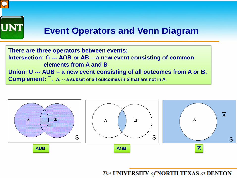
There are three operators between events: Intersection: ∩ --- A∩B or AB – a new event consisting of common elements from A and B Union: U --- AUB – a new event consisting of all outcomes from A or B. Complement: ¯, A, -- a subset of all outcomes in S that are not in A.

Event Operators and Venn Diagram

AUB A∩B A

S S S

The UNIVERSITY of NORTH CAROLINA at CHAPEL HILL

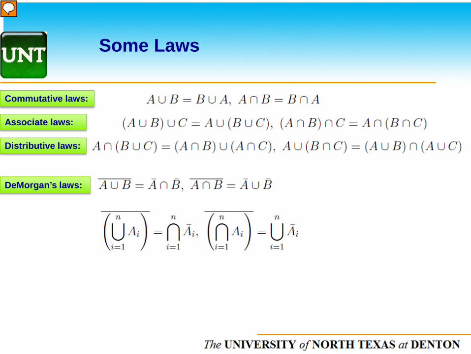
Commutative laws:

Associate laws:

Distributive laws:

DeMorgan’s laws:

Some Laws

The UNIVERSITY of NORTH CAROLINA at CHAPEL HILL

Part 2. Definition of Probability

The UNIVERSITY of NORTH CAROLINA at CHAPEL HILL

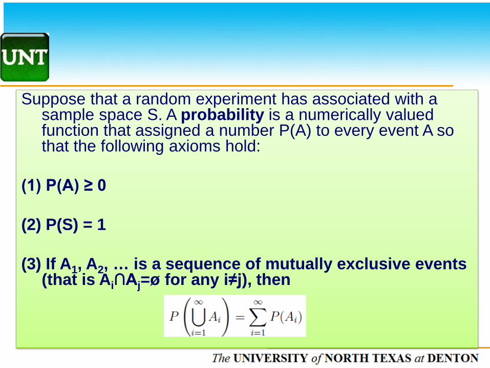
Suppose that a random experiment has associated with a sample space S. A probability is a numerically valued function that assigned a number P(A) to every event A so that the following axioms hold:

(1) P(A) ≥ 0

(2) P(S) = 1 (3) If A1, A2, … is a sequence of mutually exclusive events

(that is Ai∩Aj=ø for any i≠j), then

The UNIVERSITY of NORTH CAROLINA at CHAPEL HILL

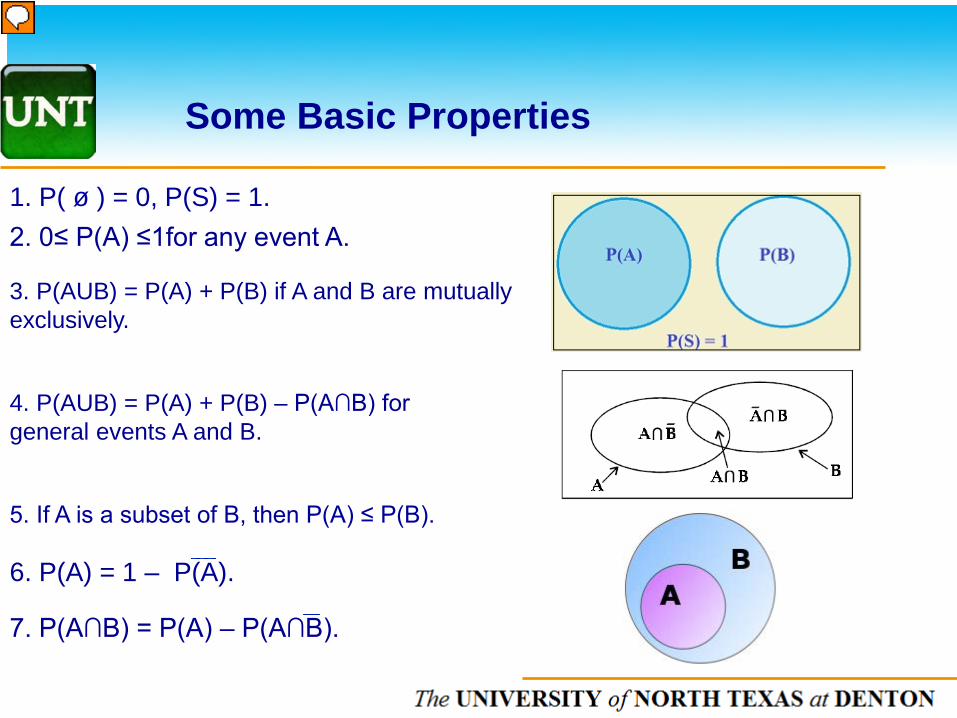
2. 0≤ P(A) ≤1for any event A.

3. P(AUB) = P(A) + P(B) if A and B are mutually exclusively.

Some Basic Properties

1. P( ø ) = 0, P(S) = 1.

5. If A is a subset of B, then P(A) ≤ P(B).

4. P(AUB) = P(A) + P(B) – P(A∩B) for general events A and B.

6. P(A) = 1 – P(A).

7. P(A∩B) = P(A) – P(A∩B).

The UNIVERSITY of NORTH CAROLINA at CHAPEL HILL

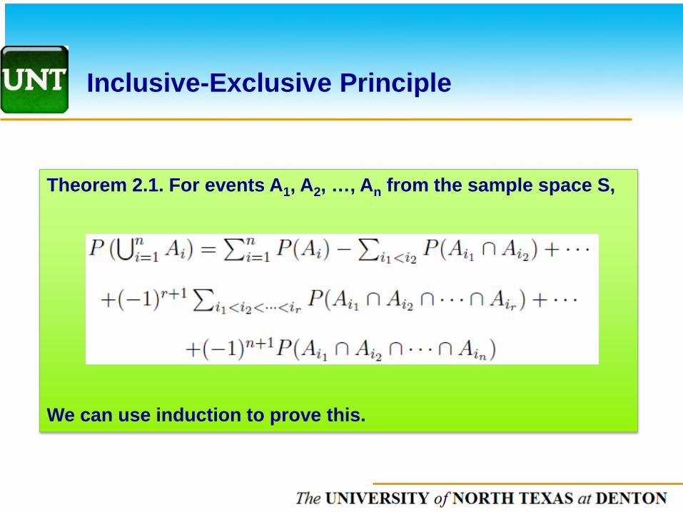
Theorem 2.1. For events A1, A2, …, An from the sample space S, We can use induction to prove this.

Inclusive-Exclusive Principle

The UNIVERSITY of NORTH CAROLINA at CHAPEL HILL

Determine the Probability Values

The definition of probability only tells us the axioms that the probability function must obey; it doesn’t tell us what values to assign to specific event.

For example, if a die is balanced, then we may think P(Ai)=1/6 for Ai={ i }, i = 1, 2, 3, 4, 5, 6

The value of the probability is usually based on empirical evidence or on careful thought about the experiment.

However, if a die is not balanced, to determine the probability, we need run lots of experiments to find the frequencies for each outcome.

The UNIVERSITY of NORTH CAROLINA at CHAPEL HILL

Part 3. Counting Rules

The UNIVERSITY of NORTH CAROLINA at CHAPEL HILL

Fundamental Principle of Counting: If the first task of an experiment can result in n1 possible

outcomes and for each such outcome, the second task can result in n2 possible outcomes, then there are n1n2 possible outcomes for the two tasks together.

Theorem 2.2

The principle can extend to more tasks in a sequence.

The UNIVERSITY of NORTH CAROLINA at CHAPEL HILL

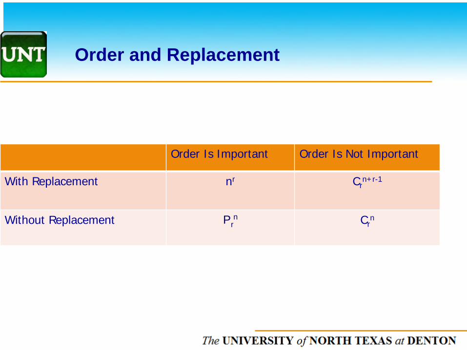
Order Is Important Order Is Not Important

With Replacement nr Crn+r-1

Without Replacement Prn Cr

n

Order and Replacement

The UNIVERSITY of NORTH CAROLINA at CHAPEL HILL

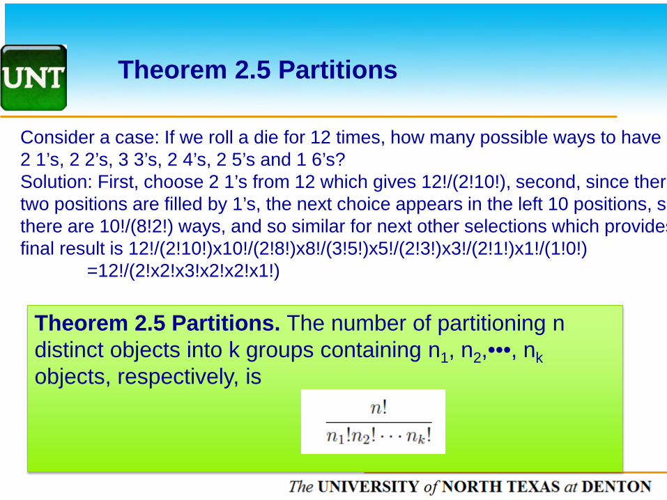
Theorem 2.5 Partitions

Consider a case: If we roll a die for 12 times, how many possible ways to have 2 1’s, 2 2’s, 3 3’s, 2 4’s, 2 5’s and 1 6’s? Solution: First, choose 2 1’s from 12 which gives 12!/(2!10!), second, since there two positions are filled by 1’s, the next choice appears in the left 10 positions, so there are 10!/(8!2!) ways, and so similar for next other selections which provides final result is 12!/(2!10!)x10!/(2!8!)x8!/(3!5!)x5!/(2!3!)x3!/(2!1!)x1!/(1!0!) =12!/(2!x2!x3!x2!x2!x1!)

Theorem 2.5 Partitions. The number of partitioning n distinct objects into k groups containing n1, n2,•••, nk objects, respectively, is

The UNIVERSITY of NORTH CAROLINA at CHAPEL HILL

Part 4. Conditional Probability and Independence

The UNIVERSITY of NORTH CAROLINA at CHAPEL HILL

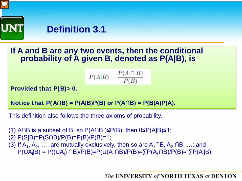
Definition 3.1

If A and B are any two events, then the conditional probability of A given B, denoted as P(A|B), is

Provided that P(B)>0. Notice that P(A∩B) = P(A|B)P(B) or P(A∩B) = P(B|A)P(A).

This definition also follows the three axioms of probability. (1) A∩B is a subset of B, so P(A∩B )≤P(B), then 0≤P(A|B)≤1; (2) P(S|B)=P(S∩B)/P(B)=P(B)/P(B)=1; (3) If A1, A2, …, are mutually exclusively, then so are A1∩B, A2 ∩B, …; and P(UAi|B) = P((UAi) ∩B)/P(B)=P(U(Ai ∩B)/P(B)=∑P(Ai ∩B)/P(B)= ∑P(Ai|B).

The UNIVERSITY of NORTH CAROLINA at CHAPEL HILL

Theorem 3.2: Multiplicative Rule. If A and B are any two events, then P(A∩B) = P(A)P(B|A) = P(B)P(A|B) If A and B are independent, then P(A∩B) = P(A)P(B).

Definition 3.2 and Theorem 3.2

Definition 3.2: Two events A and B are said to be independent if P(A∩B)=P(A)P(B). This is equivalent to stating that P(A|B)=P(A), P(B|A)=P(B) If the conditional probability exist.

The UNIVERSITY of NORTH CAROLINA at CHAPEL HILL

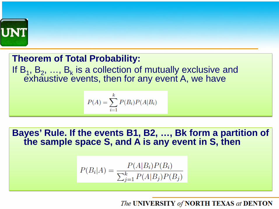
Theorem of Total Probability: If B1, B2, …, Bk is a collection of mutually exclusive and

exhaustive events, then for any event A, we have

Bayes’ Rule. If the events B1, B2, …, Bk form a partition of the sample space S, and A is any event in S, then

The UNIVERSITY of NORTH CAROLINA at CHAPEL HILL

Part 5. Probability Distribution and Expected Value

The UNIVERSITY of NORTH CAROLINA at CHAPEL HILL

A random variable X is said to be discrete if it can take on only a finite number – or a countably infinite number – of possible values x. The probability function of X, denoted by p(x), assigns probability to each value x of X so that the following conditions hold:

1. P(X=x)=p(x)≥0; 2. ∑ P(X=x) =1, where the sum is over all possible

values of x.

A random variable is a real-valued function whose domain is a sample space.

The UNIVERSITY of NORTH CAROLINA at CHAPEL HILL

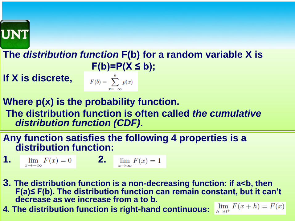
The distribution function F(b) for a random variable X is F(b)=P(X ≤ b); If X is discrete, Where p(x) is the probability function. The distribution function is often called the cumulative

distribution function (CDF). Any function satisfies the following 4 properties is a

distribution function: 1. 2. 3. The distribution function is a non-decreasing function: if a<b, then

F(a)≤ F(b). The distribution function can remain constant, but it can’t decrease as we increase from a to b.

4. The distribution function is right-hand continuous:

The UNIVERSITY of NORTH CAROLINA at CHAPEL HILL

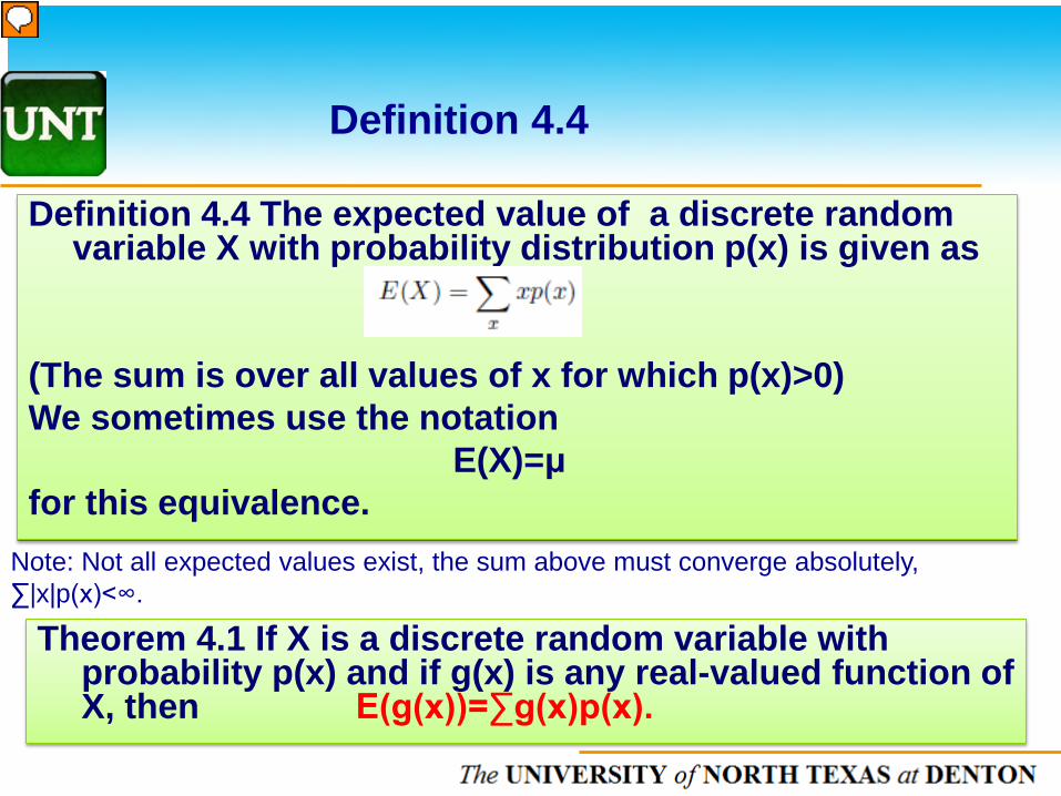
Definition 4.4 The expected value of a discrete random variable X with probability distribution p(x) is given as

(The sum is over all values of x for which p(x)>0) We sometimes use the notation E(X)=μ for this equivalence.

Definition 4.4

Note: Not all expected values exist, the sum above must converge absolutely, ∑|x|p(x)<∞.

Theorem 4.1 If X is a discrete random variable with probability p(x) and if g(x) is any real-valued function of X, then E(g(x))=∑g(x)p(x).

The UNIVERSITY of NORTH CAROLINA at CHAPEL HILL

Definitions 4.5 and 4.6

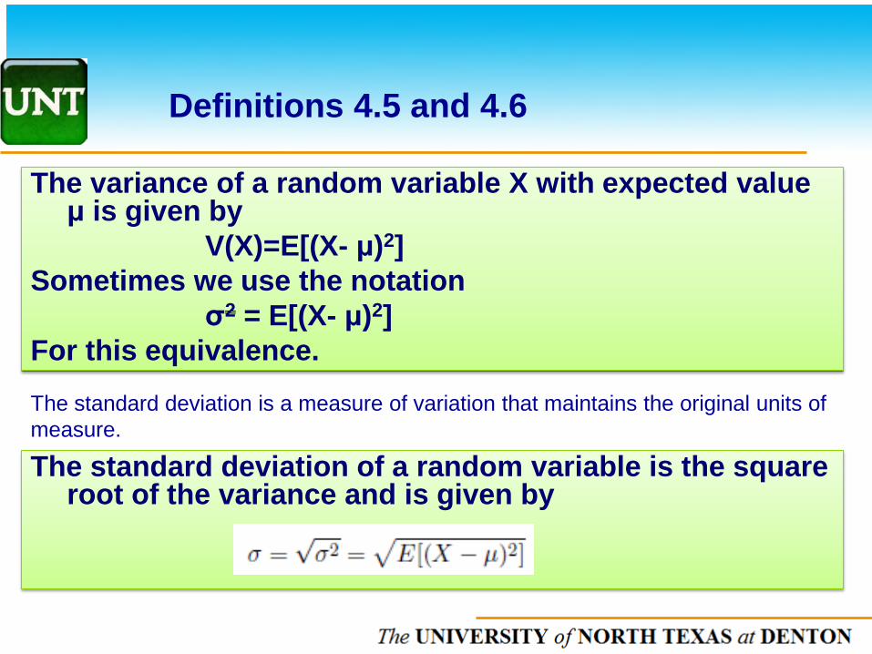
The variance of a random variable X with expected value μ is given by

V(X)=E[(X- μ)2] Sometimes we use the notation σ2 = E[(X- μ)2] For this equivalence. The standard deviation is a measure of variation that maintains the original units of measure.

The standard deviation of a random variable is the square root of the variance and is given by

The UNIVERSITY of NORTH CAROLINA at CHAPEL HILL

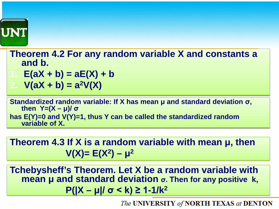
Theorem 4.2 For any random variable X and constants a and b.

1. E(aX + b) = aE(X) + b 2. V(aX + b) = a2V(X) Standardized random variable: If X has mean μ and standard deviation σ,

then Y=(X – μ)/ σ has E(Y)=0 and V(Y)=1, thus Y can be called the standardized random

variable of X.

Theorem 4.3 If X is a random variable with mean μ, then V(X)= E(X2) – μ2

Tchebysheff’s Theorem. Let X be a random variable with mean μ and standard deviation σ. Then for any positive k,

P(|X – μ|/ σ < k) ≥ 1-1/k2

The UNIVERSITY of NORTH CAROLINA at CHAPEL HILL

Part 6. Bernoulli, Binomial and Geometric Distribution

The UNIVERSITY of NORTH CAROLINA at CHAPEL HILL

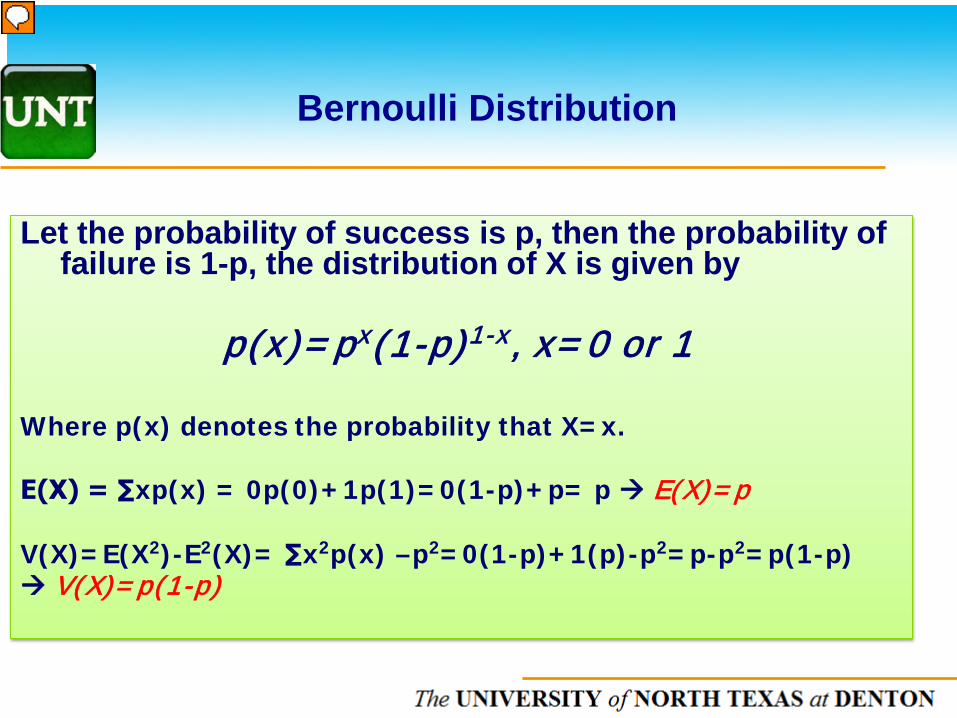
Let the probability of success is p, then the probability of failure is 1-p, the distribution of X is given by

p(x)=px(1-p)1-x, x=0 or 1 Where p(x) denotes the probability that X=x. E(X) = ∑xp(x) = 0p(0)+1p(1)=0(1-p)+p= p E(X)=p V(X)=E(X2)-E2(X)= ∑x2p(x) –p2=0(1-p)+1(p)-p2=p-p2=p(1-p) V(X)=p(1-p)

Bernoulli Distribution

The UNIVERSITY of NORTH CAROLINA at CHAPEL HILL

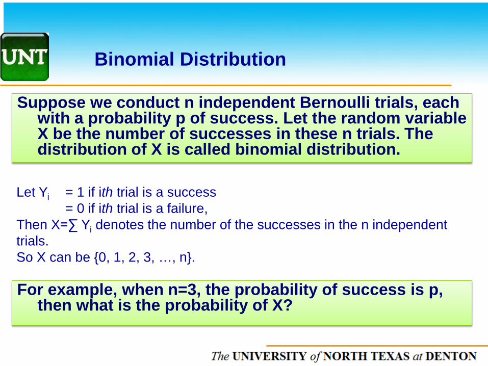
Binomial Distribution

Suppose we conduct n independent Bernoulli trials, each with a probability p of success. Let the random variable X be the number of successes in these n trials. The distribution of X is called binomial distribution.

Let Yi = 1 if ith trial is a success = 0 if ith trial is a failure, Then X=∑ Yi denotes the number of the successes in the n independent trials. So X can be {0, 1, 2, 3, …, n}.

For example, when n=3, the probability of success is p, then what is the probability of X?

The UNIVERSITY of NORTH CAROLINA at CHAPEL HILL

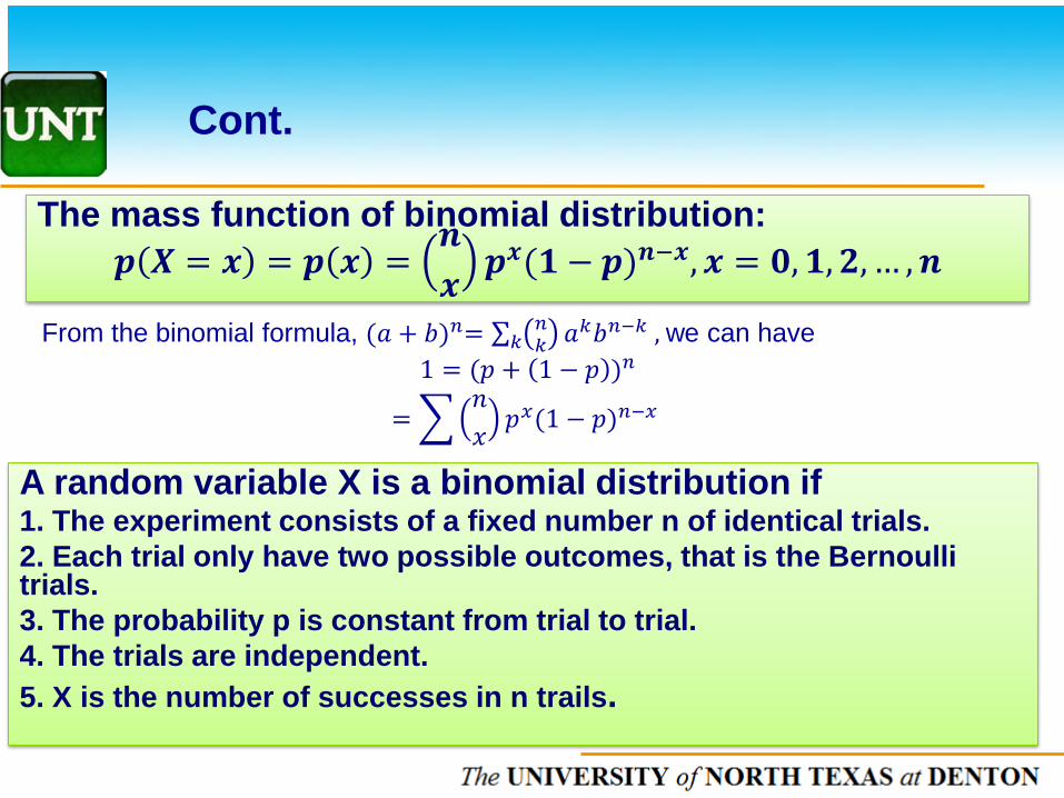
Cont.

From the binomial formula, (𝑎 + 𝑏)𝑛= ∑ 𝑛𝑘𝑘 𝑎𝑘𝑏𝑛−𝑘 , we can have

1 = (𝑝 + 1 − 𝑝 )𝑛

= �𝑛𝑥 𝑝𝑥(1 − 𝑝)𝑛−𝑥

=∑𝑝(𝑥)

The mass function of binomial distribution: 𝒑 𝑿 = 𝒙 = 𝒑 𝒙 =

𝒏𝒙

𝒑𝒙(𝟏 − 𝒑)𝒏−𝒙,𝒙 = 𝟎,𝟏,𝟐, … ,𝒏

A random variable X is a binomial distribution if 1. The experiment consists of a fixed number n of identical trials. 2. Each trial only have two possible outcomes, that is the Bernoulli trials. 3. The probability p is constant from trial to trial. 4. The trials are independent. 5. X is the number of successes in n trails.

The UNIVERSITY of NORTH CAROLINA at CHAPEL HILL

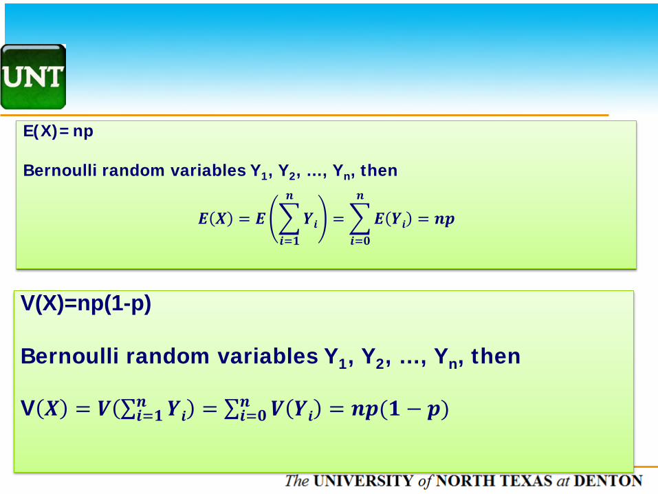
E(X)=np Bernoulli random variables Y1, Y2, …, Yn, then

𝑬 𝑿 = 𝑬 �𝒀𝒊

𝒏

𝒊=𝟏

= �𝑬 𝒀𝒊 = 𝒏𝒑𝒏

𝒊=𝟎

V(X)=np(1-p) Bernoulli random variables Y1, Y2, …, Yn, then V 𝑿 = 𝑽 ∑ 𝒀𝒊𝒏

𝒊=𝟏 = ∑ 𝑽 𝒀𝒊 = 𝒏𝒑(𝟏 − 𝒑)𝒏𝒊=𝟎

The UNIVERSITY of NORTH CAROLINA at CHAPEL HILL

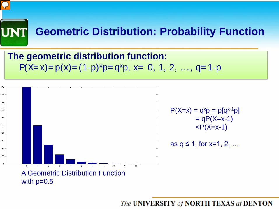
The geometric distribution function: P(X=x)=p(x)=(1-p)xp=qxp, x= 0, 1, 2, …., q=1-p

Geometric Distribution: Probability Function

P(X=x) = qxp = p[qx-1p] = qP(X=x-1) <P(X=x-1) as q ≤ 1, for x=1, 2, …

A Geometric Distribution Function with p=0.5

The UNIVERSITY of NORTH CAROLINA at CHAPEL HILL

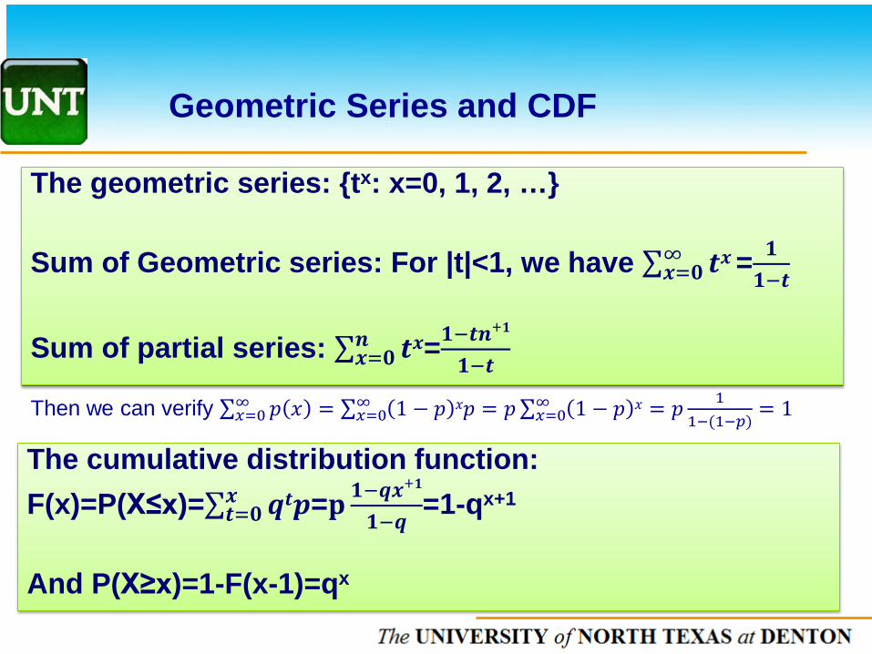
Geometric Series and CDF

The geometric series: {tx: x=0, 1, 2, …} Sum of Geometric series: For |t|<1, we have ∑ 𝒕𝒙 ∞

𝒙=𝟎 = 𝟏𝟏−𝒕

Sum of partial series: ∑ 𝒕𝒙𝒏

𝒙=𝟎 =𝟏−𝒕𝒏+𝟏

𝟏−𝒕

Then we can verify ∑ 𝑝 𝑥 = ∑ 1 − 𝑝 𝑥𝑝 = 𝑝∑ 1 − 𝑝 𝑥 = 𝑝 11−(1−𝑝)

= 1∞𝑥=0

∞𝑥=0

∞𝑥=0

The cumulative distribution function: F(x)=P(X≤x)=∑ 𝒒𝒕𝒑𝒙

𝒕=𝟎 =𝐩 𝟏−𝒒𝒙+𝟏

𝟏−𝒒=1-qx+1

And P(X≥x)=1-F(x-1)=qx

The UNIVERSITY of NORTH CAROLINA at CHAPEL HILL

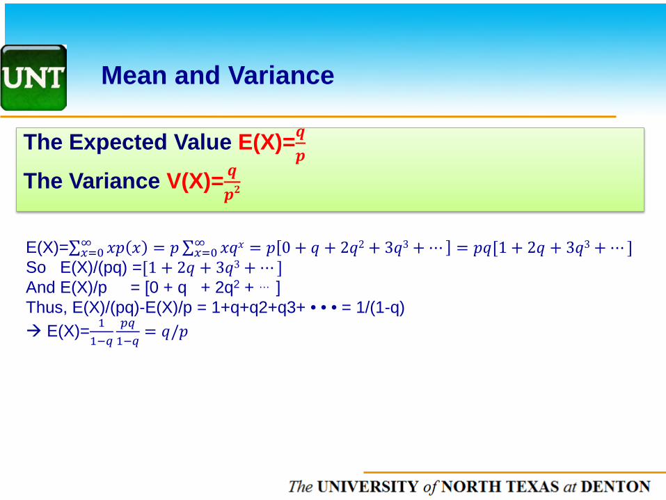
Mean and Variance

E(X)=∑ 𝑥𝑝 𝑥 = 𝑝∑ 𝑥𝑥𝑥∞𝑥=0 = 𝑝 0 + 𝑥 + 2𝑥2 + 3𝑥3 + ⋯ = 𝑝𝑥[1 + 2𝑥 + 3𝑥3 + ⋯ ]∞

𝑥=0 So E(X)/(pq) =[1 + 2𝑥 + 3𝑥3 + ⋯ ] And E(X)/p = [0 + q + 2q2 + … ] Thus, E(X)/(pq)-E(X)/p = 1+q+q2+q3+ • • • = 1/(1-q) E(X)= 1

1−𝑞𝑝𝑞1−𝑞

= 𝑥/𝑝

The Expected Value E(X)=𝒒𝒑

The Variance V(X)= 𝒒𝒑𝟐