U.S. GEOLOGICAL SURVEY CIRCULAR 1009 Review of Literature on the Finite-Element Solution of the Equations of Two-Dimensional Surface-Water Flow in the Horizontal Plane Prepared in cooperation with the United States Department of Transportation, Federal Highway Administration
Transcript
U.S. GEOLOGICAL SURVEY CIRCULAR 1009
Review of Literature on the Finite-Element Solution of the Equations of Two-Dimensional Surface-Water Flow in the Horizontal Plane
Prepared in cooperation with the United States Department of Transportation, Federal Highway Administration
Review of Literature on the Finite-Element Solution of the Equations of Two-Dimensional Surface-Water Flow in the Horizontal Plane
By JONATHAN K. LEE and DAVID C. FROEHLICH
Prepared in cooperation with the United States Department of Transportation, Federal Highway Administration
A review of computational approaches to implementing finite-element solutions of the shallow-water equations
U.S. GEOLOGICAL SURVEY CIRCULAR 1009
DEPARTMENT OF THE INTERIOR
DONALD PAUL HODEL, Secretary
U.S. GEOLOGICAL SURVEY
Dallas L. Peck, Director
Library of Congress Cataloging in Publication Data
Lee, Jonathan K. Review of literature on the finite-element solution of the equa
tions of two-dimensional surface-water flow in the horizontal plane.
(U.S. Geological Survey circular ; 1 009) "Prepared in cooperation with the United States Department of
Transportation, Federal Highway Administration." Bibliography: p. Supt. of Docs. no.: I 19.13:1009 1. Hydrodynamics-Bibliography. 2. Hydraulic
measurements-Bibliography. I. Froehlich, David C. II. United States. Federal Highway Administra-tion. Ill. Title. IV. Series.
Z5853.H9L42 1986 [TC171]
0.16.6201 '064 85-600367
Free on application to the Books and Open-File Reports Section, U.S. Geological Survey, Federal Center, Box 25425, Denver, CO 80225
CONTENTS
Abstract 1 1. Introduction 1 2. Equations of two-dimensional surface-water flow in the horizontal plane 3 3. Basic concepts of the finite-element method 5 4. Discretization of the flow domain and representation of flow variables 10
Equal-order and mixed interpolation for the shallow-water equations and their variants 10
Discontinuous interpolation 16 Resolution of the domain and network irregularity 18 Numerical integration 19 The convective terms 20
5. Treatment of boundary conditions 21 6. Time discretization 23
3 .1. Examples of two-dimensional elements 8 3.2. Two-dimensional "mapping" of some elements 9 3. 3. Finite-difference and finite-element discretizations 9 4 .1. Triangulation patterns for two-dimensional finite-element
discretizations 12 12.1. Neighborhood of node i 45 12. 2. Isoparametric quadrilateral element and center point located at
origin, i, of TJt-coordinate system 45
Review of Literature on the Finite-Element Solution of the Equations of Two-Dimensional SurfaceWater Flow in the Horizontal Plane By jonathan K. Lee and David C. Froehlich
Abstract
Published literature on the application of the finiteelement method to solving the equations of two-dimensional surface-water flow in the horizontal plane is reviewed in this report. The finite-element method is ideally suited to modeling two-dimensional flow over complex topography with spatially variable resistance. A two-dimensional finite-element surface-water flow model with depth and vertically averaged velocity components as dependent variables allows the user great flexibility in defining geometric features such as the boundaries of a water body, channels, islands, dikes, and embankments.
The following topics are reviewed in this report: alternative formulations of the equations of twodimensional surface-water flow in the horizontal plane; basic concepts of the finite-element method; discretization of the flow domain and representation of the dependent flow variables; treatment of boundary conditions; discretization of the time domain; methods for modeling bottom, surface, and lateral stresses; approaches to solving systems of nonlinear equations; techniques for solving systems of linear equations; finite-element alternatives to Galerkin's method of weighted residuals; techniques of model validation; and preparation of model input data. References are listed in the final chapter.
CHAPTER 1. INTRODUCTION
In the study of surface-water flow, vanattons in water-surface elevation and flow distribution frequently require analysis in both horizontal spatial dimensions. The finite-element method, which has been applied to fluid-flow problems only during the past 15 years, is ideally suited to modeling two-dimensional flow over complex topography with spatially variable resistance. A two-dimensional finiteelement surface-water flow model with depth and vertically averaged velocity components as dependent variables allows the user great flexibility in defining geometric features such as the boundaries of a water body, channels, islands,
dikes, and embankments. The modeler is able to use a fine network in regions where geometric or flow gradients are large and a coarse network in regions where geometry and flow are more nearly uniform. A two-dimensional finiteelement surface-water flow model eliminates the need to use empirical coefficients other than bottom-resistance coefficients in simulating subcritical flow through constrictions. In addition, the introduction of boundary conditions is easily handled in the finite-element approach.
Alternative approaches to modeling surface-water flow in two horizontal dimensions have been developed using finite-difference methods. It is useful to compare briefly the relative advantages and disadvantages of the finite-element and the finite-difference approaches.
Price and others ( 1968) show that the finite-element method requires fewer nodes and less computational time than the finite-difference method to achieve comparable accuracy in solving the one-dimensional convection-diffusion equation with a trapezoidal-rule scheme. Thacker (1978a, p. 679) shows that finite-element solutions are more accurate than finite-difference solutions in solving the equations of one-dimensional gravity-wave motion where both the depth and the grid are variable.
However, any advantage that the finite-element method has in computational time is usually lost in going from one-dimensional problems to two- and threedimensional problems because the matrices generated by the finite-element method become relatively more complex than those generated by the finite-difference method as the number of dimensions increases (Thacker, 1978b).
In particular, finite-element matrices for two- and three-dimensional problems have larger bandwidths and are less sparse than finite-difference matrices for the same problems. Moreover, the standard finite-element approach applied to time-dependent problems gives an ordinarydifferential-equation system coupled in the derivatives and requires the solution of large systems of algebraic equations at each time step, even for explicit time-stepping schemes. In addition, for an explicit time-integration scheme, the maximum allowable step size is smaller than that for the
1. Introduction 1
corresponding finite-difference scheme (Cullen, 1973, p. 18;Lynch, 1978,p. 3-10,3-16,3-17;Thacker, 1978a, p. 677, 678; Baker and Soliman, 1979, p. 311, 312).
These considerations lead Cooke (1977, p. 2) toremark: "The greatest future *** appears to lie with the approach of seeking at the outset the solution of steady state equations, where the high overhead per iterative step is offset by rapid convergence with a minimum of iterations." In light of recent developments to be discussed later in this report, Cooke's views on the use of the finite-element method for transient computations may be too pessimistic. However, in solving problems of steady free-surface flow over variable terrain, Cooke's remarks suggest that the finite-element method ought to be competitive with the finite-difference approach.
In the context of computational fluid dynamics, Roache (1975, p. 231-233) discounts the claimed geometric flexibility of the finite-element method because complex domains can be handled with regular finite-difference methods together with the use of boundary-fitted coordinates (Thames a,nd others, 1977). Although Roache's remark is valid for homogeneous domains, domain transformations are not very useful for flood plains interlaced with irregular channels. The finite-element method is much better adapted than the finite-difference method to modeling flow over variable terrain. A finite-element network can provide a much more realistic representation of topography and surface cover for a given number of nodes than can a finitedifference network. Cooke (1977, p. 29) states:
Hence, the future of the method, if any, in transient calculations, may lie in those areas where the transformation approach encounters difficulty, e.g., where the simple stretching transformations are not sufficient. Here one could envision channel flows with significant channel curvature and irregularity in cross section which varies with flow direction.
Although the finite-element method has potential advantages, most existing modeling systems based on the method are seriously flawed. A major difficulty is the large expense of using such models. Extensive manpower is required to prepare input data for model use if digitizing software is not available. Most finite-element models are costly to run in terms of both computer-core and processingtime requirements. Often, models that are less costly are applicable only under very restrictive hypotheses or are of questionable accuracy. In addition, documentation and guidelines for model use are often inadequate.
Before undertaking a program to develop an improved modeling system, it is important to survey the published literature on existing finite-element flow models. The literature on finite-difference approaches to fluid-flow modeling and other aspects of numerical analysis is also an important potential source of ideas for finite-element methods that are both more efficient and more accurate than those used in existing finite-element models.
Each subsequent chapter of this literature review is devoted to a topic important in the development of an accurate and efficient finite-element surface-water flow model.
Chapter 2 surveys the different forms of the basic equations used to describe two-dimensional surface-water flow in the horizontal plane, presents appropriate boundary conditions for each equation system, and discusses the advantages and disadvantages of the different formulations.
Chapter 3 outlines the basic concepts of the finiteelement method needed to understand the chapters that follow.
Chapter 4 discusses the discretization of the spatial domain and the representation of the dependent flow variables. Emphasis is given to the advantages and disadvantages of equal-order and mixed interpolation with various forms of the flow equations, the use of discontinuous interpolation, the effects of the resolution of the domain and network irregularity, numerical integration, and the handling of the convective terms.
Chapter 5 is devoted to ways of treating boundary conditions. Essential and natural boundary conditions and the relationship between model accuracy and the method of treating the boundary conditions are discussed.
Although many problems can be handled by steadystate analysis, it is important that a model have the capability to model unsteady flow. Moreover, time stepping is an important method for obtaining a steady-state solution. Approaches to discretizing the time domain are discussed in chapter 6. In addition, chapter 6 contains a discussion of lumping and a review of published comparisons of timestepping schemes.
Chapter 7 presents methods for modeling bottom, surface, and lateral stresses. Chapter 8 presents different approaches to handling the nonlinear terms of the flow equations, and chapter 9 discusses techniques, both direct and iterative, for solving the large systems of linear algebraic equations that are a major feature of most finite-element models.
Chapter 10 presents finite-element alternatives to Galerkin' s method of weighted residuals. Chapter 11 presents techniques for model validation. Chapter 12 discusses the preparation of model input data, including such topics as automatic network generation, the automation of the datapreparation process, and the automatic relabeling of nodes and elements. Chapter 13 presents a summary and conclusions.
Chapter 14 contains the references. Acronyms, such as FEWR 1 , refer to conference proceedings or other collections of papers and are defined at the beginning of chapter 14. Additional references are found in the reviews of Cheng (1978) and Norrie and Vries (1978).
The support of the U.S. Department of Transportation, Federal Highway Administration, is gratefully acknowledged.
CHAPTER 2. EQUATIONS OF TWO-DIMENSIONAL SURFACE-WATER FLOW IN THE HORIZONTAL PLANE
Several related sets of equations are used to describe steady and unsteady two-dimensional surface-water flow in the horizontal plane.
The most basic formulation consists of three nonlinear partial-differential equations, one for conservation of momentum in the x-direction, one for conservation of momentum in they-direction, and one for conservation of mass (Pritchard, 1971, p. 22-30):
au au au aH azo . -+U-+V-+g-+g--2 w Vsm <f> at ax ay ax ax (2.1)
-pk [a: (HTx.J+ :y (HTxy)+T~-Tf]=O, av av av aH azo . Tt+U ax +V ay +g ay +g ay +2 w U sm <f>
(2.2)
and
aH +~ (H U)+~ (H V)=O at ax ay (2.3)
where x, y =Cartesian coordinates in the positive east and
north directions, respectively, t =time,
U, V =depth-averaged velocity components in the xand y-directions, respectively,
H =total depth of water, z0 =bed elevation, p=density of water (assumed constant), w =magnitude of the angular velocity of the
Earth, <f> =latitude, g =gravitational acceleration,
T xx , T xy , =components of depth-averaged effectiveT yx , T YY stress tensor,
T~, T~ =components of surface stress (wind) in the xand y-directions, respectively, and
T~, Tt =components of bottom stress (friction) in the x- andy-directions, respectively.
Equations 2.1 through 2.3 are commonly referred to as the "shallow-water equations," and the formulation given in equations 2.1 through 2.3 is referred to as the "primitive formulation." These equations are obtained from the three-dimensional Reynolds equations for turbulent flow
by integrating with respect to the water depth under the assumption of hydrostatic pressure and by making simplifying assumptions regarding the nonlinear terms.
The first three terms of equations 2.1 and 2.2 are inertial-force terms, the first of the three representing temporal acceleration and the second and third representing convective acceleration. The fourth and fifth terms represent the pressure force due to the water-surface gradient. The sixth term represents the Coriolis force, an inertial force describing the effect of the Earth's rotation.
The seventh and eighth terms represent the combined effect of viscous stresses, Reynolds stresses, and momentum transfers due to the vertical velocity distribution (Wang and Connor, 1975, p. 64; Lean and Weare, 1979, p. 18). Some authors (Pritchard, 1971, p. 30-32; Schaffranek, 1976, p. 51) ignore the Reynolds-stress terms and handle the terms arising from vertical velocity shear in the depthaveraged equations by modifying the inertial terms of the momentum equations. This procedure requires the use of momentum-correction factors. A special case of the use of momentum-correction factors is discussed by Zienkiewicz and Heinrich (1979), who assume that the vertical velocity distribution is described by a shape function. None of the other finite-element models reviewed for this study use momentum-correction factors.
Many authors express the momentum-transfer terms in terms of the mean-flow variables by using Boussinesq' s eddy-viscosity concept, which assumes that momentum transfers due to turbulence and the vertical nonuniformity of velocity are proportional to the mean-velocity gradients. The coefficients of proportionality are referred to as "eddy viscosities." Positive and sometimes unrealistic values of eddy viscosities are often used to damp spurious oscillations in finite-element solutions of the shallow-water equations. Approaches other than viscous damping for handling unwanted oscillations are discussed in chapters 4 and 6.
The ninth and tenth terms in equations 2.1 and 2.2 represent surface and bottom stresses, respectively.
Equation 2. 3 states that the change in storage in an infinitesimally small control volume accounts for the net flux of mass into or out of the control volume.
If eddy viscosities are used to represent the turbulent stresses in equations 2.1 and 2.2, the momentum equations have a parabolic nature for positive, finite values of the Reynolds number, U0 H0/e0 , where U0 is a representative velocity, H0 a representative length, and Eo a representative value of the eddy viscosity. Large-Reynolds-number or convection-dominated flows have been the subject of much research in recent years (see reference FEMCDF), but relatively little of this research has been devoted to free-surface flows. If the eddy viscosities are set equal to zero, the shallow-water equations are a system of quasilinear hyperbolic partial-differential equations (Katapodes and Strelkoff, 1979, p. 318, 319).
2. Equations of Two-Dimensional Surface-Water Flow in the Horizontal Plane 3
A variant of the primitive shallow-water equations based on unit discharges is used by Norton and King (1973), Norton and others (1973), King and Norton (1978), and Withum and others (1979). The dependent variables are the unit discharges, UH and VH, and the depth, H. King and Norton (1978, p. 2.82) state that the advantages of this formulation include ease of representation of discharge boundary conditions and linearization of the continuity equation. Withum and others (1979, p. 703) mention the ease of ensuring the continuity of mass and momentum transfer across interelement boundaries. On the other hand, it has been observed by Teeter and McAnally ( 1981, p. 255) and the writers that a finite-element model using the unitdischarge formulation is much more sensitive to crosschannel depth changes and low eddy-viscosity values than a finite-element model formulated in terms of velocities. Unit-discharge boundary conditions are easily handled at discharge boundaries by incorporating the equations UH =constant and VH =constant into the process for handling the nonlinearities of the equations. A velocity formulation is used together with this procedure by Norton (1980).
Motivated by the experiences of earlier workers in applying finite-difference techniques to problems of computational fluid dynamics, several finite-element researchers have used different sets of equations to model twodimensional surface-water flow in the horizontal plane in an effort to obtain more accurate and efficient solution techniques.
It has been known for some time that in using a primitive-variable formulation of the Navier-Stokes equations, it is preferable to use a second-order Poisson pressure equation to enforce mass conservation rather than the primitive continuity equation (Roache, 1972, p. 194-203). In the finite-element literature, a Poisson pressure equation is used in solving the Navier-Stokes equations by Olson (1977, p. 4.191-4.194) and by Gresho, Lee, Sani, and Stullich (1978, p. 18-25).
If the nonlinear terms are neglected in equations 2.1 and 2.2, then either the velocity, U, or the depth, H, can be eliminated and the system can be reduced to a second-order wave equation in either U or H. A number of recent finiteelement models have been based on this linearized system. Fugazza and Gallati ( 1977) use the finite-element method to solve a wave equation for water-surface elevation obtained from the shallow-water equations by neglecting the convective, Coriolis, and turbulence terms. In a similar model, Mattioli ( 1981) neglects friction and assumes that the motion is harmonic but includes the Coriolis terms. Platzman (1978) uses Stokes/Helmholtz potentials instead of velocity components in his formulation of the linearized twodimensional tidal equations and shows ( 1981) that the Stokes/Helmholtz formulation is equivalent to a finiteelement wave equation. The work of other authors using a similar approach is summarized by Lynch (1978, p. 1-31-1-33).
The work discussed in the preceding paragraph forms a basis for more interesting approaches which retain all the terms of equations 2.1 through 2.3. Lynch and Gray (1979, 1980) replace the primitive continuity equation with a second-order wave continuity equation. Because the nonlinear terms are retained, the wave continuity equation couples the velocities and the depth. Thus, the wave continuity equation must be solved together with equations 2.1 and 2.2 to obtain a solution to the shallow-water equations.
As a first step, equations 2.1 and 2.2, which are given in nonconservative form , are written in conservative form by use of equation 2. 3:
a a ( ) a aH azo -(HU)+- HU2 +-(HVU)+gH-+gHat ax ay ax ax
-2 w H V sin <f> (2.4)
and
a a a ( ) aH azo - (H V)+- (H U V)+- H V2 +g H-+g Hat ax ay ay ay
+ 2 w H U sin <f> (2.5)
Then, differentiation of equation 2.3 yields
azH +_Q_[.E_ (H U)] +_Q_[.E_ (H V)] =0 (2.6) at2 ax at ay at
Substitution of equations 2.4 and 2.5 into equation 2.6 gives
a~ a{a a m a~ --- - (H U2)+- (H V U) +g H-+g H-at2 ax ax ay ax ax
-2 w H V sin,~,._![..£.. (H T )+..£.. (H T )+-r8
~ p ~ n ~ ~ x
azo 1 [a ( ) + g H ay + 2 w H u sin <f> -p ax H Tyx
+ :Y (H Ty)+r:: --rt ]}=o .
Finally, substituting equation 2.3 into equation 2. 7, and writing
(2.8)
where cb is a bottom-stress coefficient, the nonlinear wave continuity equation is obtained:
azo 1 [ a ( ) +g H --2 w H V sin<!>-- - H T OX P OX XX
+~ (H T )+Ts]}-~{~ (H U V) oy xy X oy OX
a ( ) aH ozo + iJy H V2
+ g H iJy + g H iJy + 2 w H U sin <!>
-~[:x (H Ty.)+ :y (H 7yy)+T;]}
_H u ~(cb)_H V ~(cb)=o . p ax p p iJy p
(2.9)
Lynch and Gray use the second-order equation obtained by setting T.u =Txy =Tyx =Tyy =0 in equation 2.9.
A related approach is used by Pearson and Winter (1977), who treat periodic shallow-water flow by Fourier decomposition of the dependent variables, U, V, and H, in the time domain. They obtain two coupled elliptic Helmholtz equations for each pair of Fourier coefficients of the depth, H. Le Provost and others (1981) employ a similar technique to transform the hyperbolic shallow-water equations into a set of elliptic Helmholtz equations for periodic flow phenomena. The advantages of these formulations in terms of accuracy and efficiency are discussed in chapters 4 and 6.
The appropriate boundary conditions for use with the primitive momentum equations are discussed by Wang and Connor(1975, p. 68-71), Herding (1978, p. 314, 315), and Lynch (1978, p. 1-5, 1-6). If it is assumed that the boundaries of the flow domain are fixed, and if second-order eddy-viscosity terms are not included in the momentum equations, either the normal mass flux (normal discharge) or the normal force (normal stress) must be specified at all points on the boundary of the flow domain. If eddy-viscosity terms are included in the momentum equations, an additional boundary condition is needed at all points on the boundary. Either the tangential mass flux (tangential discharge) or the tangential force (shear stress) must be specified at all boundary points. The continuity equation, used to find the elevation of the free surface, does not require any boundary conditions (Wang and Connor, 1975, p. 71).
Katapodes ( 1980) discusses boundary conditions for flows that are not completely subcritical. Pearson and Winter ( 1977) present appropriate boundary conditions for an open tidal boundary that account for landward tidal reflec-tion.
Most researchers solving two-dimensional flow problems that do not involve a free surface convert the primitive equations of flow to a parabolic vorticity-transport equation and an elliptic stream-function equation. Among the researchers who use a vorticity-stream-function finite-element formulation to study viscous incompressible flow in two dimensions are Cheng (1972), Baker (1973), Brebbia and Smith (1977), Olson and Tuann (1978a), Tuann and Olson (1978), and Moult and others (1979). Unlike the twodimensional Navier-Stokes continuity equation, however, equation 2.3 couples the depth and the velocity components. Because of this, the vorticity-stream-function approach cannot be applied to transient shallow-water flow.
Only in the case of steady flow, where the time derivatives in equations 2.1 through 2.3 vanish, is it possible to apply a vorticity-stream-function approach to twodimensional surface-water flow. This is of considerable interest because it is possible to handle as steady state most problems involving flood-plain constrictions. Franques (1971) and Franques and Yannitell (1974) develop such an approach. They define the stream function, \jl, by
iJ\jl =-H V and ~=H U ox . iJy (2.10)
and the vorticity, ,, by
a a '=-(H U)--(H V)
iJy ox (2.11)
By neglecting the convective term in the vorticity-transport equation, the authors obtain a nonlinear elliptic partialdifferential equation in \jl. The validity of the assumption that the convective term in the vorticity-transport equation can be neglected deserves further investigation. Boundary conditions consist of constant values of \jl at lateral boundaries and zero values of the normal derivative of \jl at upstream and downstream boundaries, which are assumed to be normal to the flow. Water-surface elevations are obtained from Bernoulli's equation.
CHAPTER 3. BASIC CONCEPTS OF THE FINITE-ELEMENT METHOD
The finite-element method is a numerical procedure for solving the differential equations encountered in problems of physics and engineering. Although it was originally devised to analyze structural systems, the finite-element method has developed into an effective tool for evaluating
3. Basic Concepts of the Finite-Element Method 5
a wide range of problems in the field of continuum mechanics. This development has been encouraged primarily by the continued advancement of high-speed digital computers, which provide a means of performing rapidly the many calculations involved in the method.
The fundamental concept of the finite-element method is that any smooth quantity can be approximated by a discrete model composed of a set of piecewise-smooth functions which are defined over a finite number of subdomains called elements. The piecewise-smooth functions are called interpolation, shape, trial, or basis functions, are described in terms of the values of the smooth quantity at a finite number of points in its domain, and are typically polynomials of at most the third or fifth degree. The points at which the quantity is defined are called nodes and are usually located along the element boundaries, where adjacent elements are considered to be connected, although some nodes may be positioned in the element interiors.
The nodal values of the quantity being modeled along with the selected interpolation functions completely describe the variation of the quantity within each element. For the finite-element solution of the problem, the nodal values become the unknowns. The behavior of the solution throughout the assemblage of elements is described by the interpolation functions once the unknown nodal quantities are found.
Clearly, interpolation functions cannot be selected arbitrarily; they should be able to approximate the true distri· bution of the field variable as closely as possible. In addition, at element boundaries the field variable and any of its partial derivatives up to one order less than the highest order derivative of the equation being solved must be continuous. This is known as the compatibility requirement. Elements whose interpolation functions satisfy this requirement are known as compatible or conforming elements. Another condition that must be met is that as the element size shrinks to zero, values of the field variable and of all its partial derivatives up the highest order appearing in the equation being solved must be constant over an infinitesimal part of the solution domain. This is known as the completeness requirement.
At this point it is helpful to introduce a standard defi,. nition and notation to describe the degree of continuity of the interpolation function. If the interpolated variable is continuous, it is said to have C0-continuity. If first derivatives are continuous, the interpolation function is said to have C 1-continuity. Continuous second derivatives imply C2-continuity, and so on.
Suppose the functions appearing under the integrals of the element equations contain derivatives up to the (r + 1 )st order. To satisfy the compatibility requirement, the interpolation functions must be cr-continuous at element boundaries. The completeness requirement is met if the interpolation functions are cr+ 1-continuous within each element. These requirements for interpolation functions representing
the behavior of a field variable are usually sufficient to ensure convergence to the solution as element size decreases.
Once the finite-element model has been established (that is, once the elements and their interpolation functions have been chosen), the derivation of the element equations may be achieved by direct methods, variational methods, or weighted-residual methods.
Direct methods for deriving finite-element equations are based on direct physical reasoning but can be applied only for relatively simple problems and element shapes. However, the finite-element equations that are found by direct physical reasoning can also be derived by minimizing an energy functional (Becker and others, 1981 , p. 60) with respect to the nodal variables. Thus, a general method for formulating the finite-element equations is obtained by applying variational principles governing the particular problem of interest.
The variational approach to deriving element equations is the most widely used and is the most convenient when a classical variational statement exists for a particular problem. However, many practical problems are encountered for which classical variational principles are unknown. In these cases, more generalized procedures must be used to derive the element equations.
Weighted-residual methods are general techniques for obtaining approximate solutions to linear and nonlinear partial-differential equations and include collocation, least squares, and Galerkin methods. In all of these, the unknown solution is approximated by a set of interpolation functions containing adjustable constants or functions. The chosen constants or functions define the type of weighted-residual method and attempt to provide the "best" approximation of the exact solution. Although the methods of weighted residuals offer a more general means of formulating the element equations, they are not directly related to the finite-element method.
To be more specific, the differential equation for a problem can be written as
L u-J=O (3.1)
on the domain R, where L is a differential operator, u is the field variable, and f is a known function. The dependent variable, u, is approximated as
m
u=u= 2: N;U; '
i=I (3.2)
where theN; are the assumed interpolation functions and the u; are the unknown nodal variables. When u is substituted into equation 3. 1 , it is unlikely that the equation will be satisfied; in fact, the trial solution is defined as
L u-J=e, (3.3).
where e is the residual or error because the solution is only approximate. The method of weighted residuals seeks to determine them unknowns, u;, such that the error, e, over the entire solution domain is as small as possible (Huebner, 1975, p. 106-110). One way of accomplishing this is to form a weighted average of the error and require that this weighted average vanish over the solution domain, R. If m linearly independent weighting or test functions, W;, are chosen, and the integral
f W; edR R
(3.4)
is required to vanish for each of the weighting functions (that is, e is required to be orthogonal to the space spanned by theW;), then e equals zero in some average sense. Once the weighting functions have been specified, a set of m simultaneous equations remains to be solved for the unknown nodal variables.
The particular weighted-residual methods differ from one another in the choice of the weighting functions. The technique most often used to derive finite-element equations is known as Galerkin' s method. In this method, the weighting functions are chosen to be the same as the interpolation functions of the trial solution, that is, W; =N; for i = 1, 2, ... ,m. Thus Galerkin's method requires that
f N; (L u -J) dR =0; i = 1, 2, ... ,m . (3.5) R
The left-hand side of equation 3.5 can be written as the sum of expressions governing the behavior of equation 3.1 on individual elements. The variable u can be approximated on an element as
n
u<e>="" N~e) u~e> LJ I I '
i = 1 (3.6)
where the superscript (e) denotes the restriction of the relevant variable or function to the element and n is the number of unknown nodal variables assigned to the element. Then the left-hand side of equation 3.5 can be written as the sum of expressions of the form
A set of such expressions can be developed for each element of the system and then combined. This assembly of the element, or local, expressions results in a set of global
algebraic equations, which must be solved simultaneously. The assembly process will not include any spurious contributions as long as the interpolation functions, N;, satisfy the compatibility requirement discussed earlier.
In many cases, it is possible to reduce the order of derivatives contained in the governing differential equations by applying integration by parts to the integral expressions of the finite-element equations. Hence, the interpolation functions will be required to satisfy a less stringent compatibility condition. Not only will the choice of approximating functions be less restricted, but the surface or line integrals that arise from integration by parts provide a convenient means of applying certain boundary conditions of the problem. Such boundary conditions are called natural boundary conditions. These boundary integral terms are then usually moved to the right-hand side of the system of finite-element equations. Although these boundary terms will appear in the equations for every element of the system, they need only be evaluated on boundary elements since all internal contributions will cancel. Essential boundary conditions can be applied to the combined system of equations once the assembly process is complete. Essential boundary conditions are those that the nodal values are required to satisfy directly. They are usually introduced by eliminating the finiteelement equations that govern the relevant nodal variables.
The basic idea of the finite-element method is that a solution domain of arbitrary shape can be discretized by assemblages of elements in such a way that a sequence of approximate solutions defined on successively more refined discretizations will converge to the exact solution of the governing differential equations. In most cases, these elements are geometrically fairly simple. Common twodimensional elements are shown in figure 3 .1. The threenode triangle is the simplest element that can be used to define the linear variation of a quantity in two dimensions. Because of its simplicity and its ability to model domains of nearly any shape, it is the most frequently used twodimensional finite element. The four-node quadrilateral is another commonly used linear two-dimensional element and may be formed directly or by the combination of two or four linear triangles. Elements with additional nodes are used to define higher order approximating functions. For example, the 6-node triangle can be used to model the quadratic variation of a field variable and the 10-node triangle can describe a cubic variation. Other higher order elements are possible but are not frequently used.
It is also possible to construct elements with curved sides. These elements, two of which are shown in figure 3.2, are useful in representing geometries of complex shape by allowing curved boundaries to be modeled with fewer elements. Such an element is formed by mapping a "parent" element defined in some local coordinate system into the distorted shape in the global coordinate system. The finiteelement equations are then evaluated by integrations in the local coordinate system over the parent element (Huebner,
1975, p. 186). The element geometry is described by polynomial functions in the same manner as the field variables using global coordinates as the nodal quantities. If the interpolation functions for the element geometry are of the same order as those for the field variables, the element is said to
be isoparametric. If, on -the other hand, a lower order polynomial is used to describe the geometry than is used for the field variable, the element is called subparametric. Superparametric elements are those whose geometry is defined by a function of higher order.
D "Parent" elements in
local coordinates Curved-sided elements in Cartesian coordinates
Figure 3.2. Two-dimensional "mapping" of some elements.
Like other numerical techniques for solving boundary-value problems, the finite-element method is based on the concept of discretization. In contrast to finitedifference methods, however, the idealization portrays the body as continuous and the solution is given as a piecewisesmooth approximation to the governing differential equation over the entire assemblage of elements. Since these elements can vary widely in size and shape within a single network, they can be used to represent exceedingly complex geometries. (For accuracy reasons, such variation in size and shape should be gradual.) In addition, the finite-element method has proved successful in modeling systems composed of various types of materials having very complicated properties.
The more commonly known finite-difference method, on the other hand, is based on a pointwise approximation to the governing differential equation. In this method, the differential equation is replaced by a difference equation written at a discrete set of points over some continuous region. Usually, these points are arranged in a uniform rectangular grid. When irregular geometries are encountered, however, boundaries must be represented in a discontinuous "stairstep" fashion within the model. This creates a loss of accuracy near these boundaries, where the solution is often of greatest importance. In addition, the grid spacing required to represent the most detailed portions of the study region must be used throughout the entire solution domain unless special mapping procedures are used. In many cases, numerical detail is wasted in areas where a larger grid spacing would suffice.
~ I--
r---....~
)v \ :\ /.
/~ r--: 1--~ / ' /
/.
\ /
" v :-.....
............ ~ / ;...-'
----:____ -~ A
B
Figure 3.3. Finite-difference and finite-element discretizations: (A) Typical finite-difference grid, and (8) Typical finiteelement grid.
As an example of how a finite-difference model and a finite-element model might be used to represent a complex geometrical shape, consider the two-dimensional body in figure 3. 3. A uniform finite-difference grid reasonably covers the region, but the boundaries must be approximated in a highly discontinuous manner. On the other hand, the finite-element representation, using the simplest twodimensional element, the three-node triangle, gives a much better approximation to the region and requires fewer grid points. Also, the boundary is approximated much more smoothly since it is represented by a series of straight lines.
Another advantage of the finite-element method is the relative ease with which boundary conditions of the problem can be handled. Many physical problems have boundary
3. Basic Concepts of the Finite-Element Method 9
conditions involving derivatives and, in general, the boundary of the region being modeled is irregularly shaped. Using finite-difference techniques, each boundary condition involving a derivative must be approximated by using special devices such as noncentered difference equations or fictitious external grid points. Since the finite-element method generally includes the boundary conditions as integrals in a functional which is being minimized, application presents no special problem.
Additional information on the theory and application of the finite-element method can be found in the books of Desai and Abel (1972), Strang and Fix (1973), Huebner (1975), Segerlind (1976), Pinder and Gray (1977), Zienkiewicz (1977), Chung (1978), Becker and others (1981), and Carey and Oden (1983).
CHAPTER 4. DISCRETIZATION OF THE FLOW DOMAIN AND REPRESENTATION OF FLOW VARIABLES
In simulating both steady and unsteady flow over nonuniform terrain, the method of discretizing the spatial domain requires the most careful consideration. The spatial discretization determines how well variations in topography and surface cover can be resolved and thus how well the flow model is able to resolve velocity and water-surfaceelevation gradients. The type of discretization used is related to the ability of the model to accurately approximate the solution of the continuous flow equations.
The representation of the dependent variables of surface-water flow is closely related to the type of spatial discretization used and in tum influences both the numerical methods that can be used to solve the resulting equation systems and the accuracy of the discrete solution.
In this chapter, we review the experience of researchers who have used varying methods of spatial discretization in solving the shallow-water equations and variants of the shallow-water equations. We also review the more extensive literature concerning the finite-element solution of the Stokes and Navier-Stokes equations. Information obtained from this work can suggest useful techniques that may be applied to the shallow-water equations.
Equal-Order and Mixed Interpolation for the Shallow-Water Equations and Their Variants
Many researchers solving the primitive shallow-water equations by finite-element methods use the same order of interpolation for both the velocity components and depth (equal-order interpolation). Wang and Conner (197 5), Kelley and Williams (1976), Harrington and others (1978), Kawahara, Nakazawa, Ohmori, and Hasegawa (1978), Kawahara, Takeuchi, and Yoshida (1978), and Tanaka and
others ( 1980) use equal-order linear interpolation on triangles in solving the primitive shallow-water equations, while Brebbia and Partridge (1976a, 1976b) and Partridge and Brebbia ( 1976) use equal-order quadratic interpolation on triangles. Malone and Kuo (1981) use equal-order bilinear interpolation on four-node quadrilaterals, Taylor and Davis ( 1975) use equal-order quadratic interpolation on eight-node quadrilaterals, and Gray (1977) uses equal-order biquadratic interpolation on nine-node quadrilaterals.
Researchers using equal-order interpolation report significant problems in obtaining solutions free of shortwavelength noise and resort to a variety of techniques for dealing with this problem. Gray (1977, p. 4.45) reports oscillations in his water-surface-elevation solution. Wang and Connor (1975), Tanaka and others (1980), and Malone and Kuo ( 1981) report results at element centroids, in an attempt to filter out internode oscillations. Lynch (1978, p. 4-19) shows that reporting results at element centroids has a significant smoothing effect on the solution. Walters (written commun., 1984) has pointed out that this procedure is equivalent to sampling near the nodal points of an almoststationary short-wavelength oscillation. Brebbia and Partridge (1976b), Kawahara, Nakazawa, Ohmori, and Hasegawa (1978), and Malone and Kuo (1981) use smoothing to obtain stable solutions. Wang and Connor (1975), Kelley and Williams (1976), Kawahara, Nakazawa, Ohmori, and Hasegawa (1978), Kawahara, Takeuchi, and Yoshida (1978), and Tanaka and others (1980) use eddyviscosity terms with equal-order interpolation to eliminate short-wavelength noise from the solution. Gray (1980, p. 1.126-1.128) observes that, in addition, Kawahara, Takeuchi, and Yoshida (1978) use a time-stepping scheme that is extremely dissipative. Brebbia and Partridge (1976a, 1976b) use unrealistically large bottom friction to obtain results without noise. Harrington and others (1978) use artifically large bottom friction, eddy-viscosity terms, and a dissipative fully implicit time-stepping scheme to damp spurious oscillations.
Workers solving the primitive Navier-Stokes equations have also used the same order of interpolation for both velocities and pressure. It is now recognized, however, that the use of equal-order interpolation is the cause of spurious oscillations in the pressure solution, as is discussed in detail below. Various approaches have been adopted to solve this problem. Because these approaches are useful to researchers applying finite-element methods to the shallow-water equations, they are reviewed at length below.
A widely used approach for eliminating pressure oscillations is the use of mixed interpolation, in which a lower order of interpolation is used for the pressure than for the velocity components. Hood and Taylor (1974) ascribe the need for mixed interpolation to error consistency. They suggest that the order of error associated with each dependent variable must be the same. Bratianu and Atluri (1980) state that the ratio of discrete constraint (continuity) equations to
discrete momentum equations should be as close as possible to the continuum value of 0. 5. For several meshes with small numbers of elements, they show that mixed interpolation satisfies this condition quite well and gives better results than equal-order interpolation. Schneider and others (1978) and Carey (1980) point out that the number of discrete constraint equations must not exceed the number of discrete momentum equations to avoid overconstraint of the discrete system.
Carey (1980, p. 4.68), however, remarks that mixed interpolation is no guarantee that overconstraint will be avoided:
The linear velocity-constant pressure triangle offers a convenient example. The velocity is conforming so the velocity nodes are at the vertices and the pressure node at the centroid. In an initial coarse mesh the dimension of the velocity space may exceed that of the pressure space. As the mesh is refined uniformly the number of elements increases faster than the number of nodes until the number of pressure degrees-of-freedom exceeds the number of degrees-of-freedom for velocity. This implies that the number of "constraint equations" in the finite element system increases relative to the "equilibrium equations" and the problem becomes overconstrained.
Although these observations are valid, they do not adequately explain the difficulties that mixed interpolation is used to solve. Olson (1977) and Olson and Tuann (1978b) suggest that the real problem is that the system matrix resulting from finite-element discretization of the primitive Navier-Stokes equations is nonpositive definite because the continuity constraint is uncoupled from the momentum equations. Spurious pressure modes arise because of this and mask the desired pressure solution. Mixed interpolation can be used to eliminate the spurious modes in some cases.
It is also known that solving different forms of the equations of flow eliminates the difficulties that mixed interpolation is used to solve. Schneider and others ( 1978) observe that equal-order interpolation is successful if the primitive continuity equation is replaced by a Poisson pressure equation. Another approach is to replace the primitive equations with the vorticity-stream-function equations. Reddy and Warburton (1980) adopt this approach and successfully interpolate both vorticity and stream function with bilinear interpolation functions on four-node quadrilateral elements. This scheme is chosen on the basis of the observation of Jesperson (1974) that bilinear interpolation on a patch of rectangular elements is equivalent to a scheme of Arakawa's, which is known to conserve mean kinetic energy, mean vorticity, and mean square vorticity.
Additional research into spurious pressure modes generated by some fmite-element techniques for solving the Navier-Stokes equations has accelerated in the last few years and is leading to a deeper understanding of the problem.
Huyakorn and others ( 1978) report the results of numerical experiments to compare the accuracy of several
mixed-interpolation elements in solving the Navier-Stokes equations. The elements studied are the four-one, eightfour, and nine-four rectangles and the six -three triangles. (The first number refers to the number of velocity nodes, the second to the number of pressure nodes. All interpolation is continuous except that for the pressure in the four-one rectangle.) The four-one element exhibits a spurious "checkerboard" pressure mode in an example involving steady free thermal convection. This spurious mode is suppressed by specifying pressures or total stresses on at least one boundary. The nine-four rectangle is the most accurate for both velocities and pressures. The performance of the six-three triangles depends on the triangulation pattern used. Better results are obtained when six nodes are connected to each interior node (fig. 4.1A) than when alternately four and eight nodes are connected to each interior node (fig. 4.1C). These results also illustrate that solution quality usually decreases as the irregularity of the network increpses. Hence, one must be careful in inferring information about specific elements from their behavior in particular arrangements.
Hansen and Flotow (1982) discuss standard and upwind convection operators for the same two triangulation patterns studied by Huyakorn and his coworkers. The solutions depend on the triangulation pattern used for both standard and upwind elements (see the section "The Convective Terms"). The differences are large only for Reynolds numbers greater than 100 because only the convection operator is nonsymmetric. For Reynolds numbers less than 100, there is little dependence on triangulation pattern or upwind weighting scheme.
Carey and Oden (1983, p. 96-138) and Oden and Carey (1983, p. 99-150) explain the success of some types of mixed interpolation for the steady Stokes equations, for which the pressure-mode problem is the same as for the Navier-Stokes equations. The problem is put into the context of constrained minimization of an appropriate discrete functional using a Lagrange multiplier. The Lagrange multiplier turns out to be the hydrostatic pressure, and, in general, the approximate velocity and pressure solutions lie in different function spaces. Stability and convergence are obtained for velocity and pressure spaces whose elements satisfy a discrete Ladyzhenskaya-Babuska-Brezzi (LBB) inequality. Bercovier and Pironneau ( 1977) show that this inequality is satisfied for the following conforming approximations: quadratic interpolation for velocities and linear interpolation for pressure on triangles, and biquadratic interpolation for velocities and bilinear interpolation for pressure on rectangles. In addition, the domain is required to be a polygon in the plane, and not more than one element side for triangles or two for rectangles can coincide with the boundary of the domain. On the other hand, linear interpolation for velocities and constant interpolation for pressure on triangles fails to satisfy the LBB condition (Carey, 1980, p. 4.70).
4. Discretization of the Flow Domain and Representation of Flow Variables 11
D
B E
Figure 4.1. Triangulation patterns for two-dimensional finite-element discretizations: (A) One-directional mesh with six nodes connected to each interior node and diagonals of negative slope; (8) One-directional mesh with six nodes connected to each interior node and diagonals of positive slope; (C) Mesh with alternately four and eight nodes connected to each interior node; (0) Hexagonal mesh with six nodes connected to each interior node; (f) Mesh of (0) rotated 90 degrees; (f) Two-directional mesh with six nodes connected to each interior node and diagonals of alternating positive and negative slope.
Fix and others (1979) and Fix (1980) present an alternative approach for obtaining stable and convergent solutions to the Navier-Stokes equations. These authors establish a necessary relationship between the pressure and velocity function spaces and show that the velocity spaces must satisfy a certain decomposition property.
By studying the behavior of the algebraic equations derived by applying the finite-element method to small
patches of elements for steady Stokes flow, Sani, Gresho, Lee, and Griffiths ( 1981) and Sani, Gresho, Lee, Griffiths, and Engelman ( 1981) are able to characterize conditions giving rise to spurious pressure modes for a number of elements involving both equal-order and mixed interpolation. Since the pressure-mode problem for the steady Stokes equations is equivalent to the pressure-mode problem for the steady Navier-Stokes equations, and since the steady
Navier-Stokes equations are equivalent to the steady shallow-water equations with pressure corresponding to depth and other appropriate identifications (Zienkiewicz and Heinrich, 1979, p. 681), the characterizations made by Sani and his coworkers apply equally well to the steady shallowwater equations. It must be noted, however, that the correspondence between the steady Navier-Stokes equations and the steady shallow-water equations requires that the distance, h, to the bed from a horizontal reference plane be much greater than the distance, 11· from the water surface to the reference plane.
Mixed interpolation on isoparametric quadrilaterals with continuous bilinear velocity and discontinuous constant pressure exhibits a spurious "checkerboard" pressure mode. (The discontinuous pressure approximations considered by Sani and his coworkers use Gauss-point pressure nodes.) Filtering and smoothing techniques (Sani, Gresho, Lee, and Griffiths, 1981, p. 36-38) must be used to obtain useful pressures. Equal-order interpolation with continuous bilinear velocity and either continuous or discontinuous bilinear pressure on isoparametric quadrilaterals displays multiple pressure degeneracies. The situation is worse with equalorder interpolation on higher order elements.
Mixed interpolation with continuous biquadratic velocity and continuous bilinear pressure has no spurious pressure modes. Mixed interpolation with continuous biquadratic velocity and discontinuous bilinear pressure exhibits one spurious pressure mode, which can be suppressed by avoiding the specification of the tangential component of velocity on the boundary of the domain. A pressure filter is described by Sani, Gresho, Lee, Griffiths, and Engelman (1981, p. 177, 178) for obtaining physical pressures in this case.
The continuous eight-node "serendipity" velocity element with continuous bilinear pressure exhibits no spurious pressure modes. However, the element has other difficulties related to the imbalance in the number of nodes along the side and through the center of the element. If discontinuous bilinear pressure is used with the same velocity element, at least three spurious modes occur. Mixed interpolation with continuous biquadratic velocity and discontinuous linear instead of discontinuous bilinear pressure (the nine-three element) has no spurious modes. This element is also discussed by Engelman, Sani, Gresho, and Bercovier (1982).
These results are related to those of Bercovier and Pironneau ( 1977) by the fact that the existence of spurious pressures modes implies that the LBB inequality does not hold (Carey, 1980, p. 4.68, 4.69; Sani, Gresho, Lee, Griffiths, and Engelman, 1981, p. 180).
Jackson and Cliffe (1981) examine in detail the spurious pressure modes on quadrilaterals with continuous ninenode velocity interpolation and continuous eight-node pressure interpolation and show that the spurious modes can be suppressed by including one eleven-eight element in a grid. The overall ratio of pressure unknowns to velocity un-
knowns is much closer to the continuum ratio of 0. 5 than it is for the continuous nine-four, eight-four, or six-three elements. Jackson and Cliffe (1981, p. 1677) state: "It seems reasonable to expect the above methods to give improved performance over the 9-node full biquadratic velocity interpolation 4-node bilinear pressure element, due to the higher order of approximation of the pressure, together with the fact that incompressibility is more closely enforced." Jackson and Cliffe point out that this suggests the possibility of using such special elements to suppress spurious modes with equal-order interpolation.
The effect of isoparametric transformations on spurious pressure modes has been studied by both Sani and his coworkers and Jackson and Cliffe. Sani, Gresho, Lee, and Griffiths (1981, p. 32-36) note that a distorted isoparametric network gives rise to an "impure" spurious pressure mode for combinations of element types and boundary conditions supporting "pure" spurious pressure modes. These impure modes can be manifested in large velocity errors. When no spurious pressure modes are present, Jackson and Cliffe ( 1981, p. 1677) observe that a "small" isoparametric transformation cannot lead to such modes. It is apparently unknown how large the "small" can be without introducing spurious modes.
The remainder of this section is devoted to the shallowwater equations, which differ from the Navier-Stokes equations in several respects. The behavior of solution algorithms for the shallow-water equations is complicated by the coupling of depth (or water-surface elevation) and velocities in the continuity equation, which now contains the partial derivative of depth with respect to time. This added term is responsible for the phase speed (the ratio of the temporal frequency to the wavenumber in Fourier analysis) being finite for the shallow-water equations but infinite for the Navier-Stokes equations and leads to different spurious modes for the two systems of equations (R.A. Walters, written commun., 1984). In spite of these differences, many of the approaches that are useful for the Navier-Stokes equations are also useful for the shallow-water equations.
Success in solving the Navier-Stokes equations with certain types of mixed interpolation led researchers working with the shallow-water equations to apply the same technique. Quadratic interpolation for velocity components and linear interpolation for depth or water-surface elevation on triangles is used by Norton and King (1973), Norton and others (1973), Tseng (1975a, 1975b), King and Norton (1978), Walters and Cheng (1978, 1980), Norton (1980), and Gee and MacArthur ( 1982). Thien pont and Berlamont ( 1980) use quadratic interpolation for velocity components and bilinear interpolation for depth on eight-node quadrilateral elements (see p. 4.12).
In the last several years, research on the application of finite-element methods to the shallow-water equations has focused on the application of analytical techniques to understand the behavior of solution algorithms.
4. Discretization of the Flow Domain and Representation of Flow Variables 13
Gray and Lynch (1977, 1979), Lynch (1978), and Lynch and Gray (1979) apply Fourier methods to study various time-stepping schemes for the shallow-water equations with both the primitive and wave continuity equations. .These studies are done in the context of the linearized onedimensional shallow-water equations with a linearized friction term. Equal-order interpolation is used for velocity and water-surface elevation. These authors observe that most schemes using the primitive continuity equation have serious problems with short-wavelength noise and that none of
·the schemes using the primitive continuity equation propa-. gate 2dx waves, that is, waves having a wavelength twice
the grid spacing, dx (Gray and Lynch, 1979, p. 54, 55). Lynch and Gray (1979, p. 214-217) show that schemes using the wave continuity equation propagate 2dx waves and imply that this fact is related to the capability of waveequation models to yield water-surface-elevation solutions without spurious oscillations in cases where shortwavelength modes are forced. It remained for Platzman to more fully explain the short-wavelength-noise problem.
Platzman ( 1978, 1981) studies the effect of spatial discretization on model response for the linearized shallowwater equations without friction in one and two dimensions. (Platzman does not discretize time.) He considers both primitive and derivative formulations. The derivative formulation is obtained by using Stokes/Helmholtz potentials and is equivalent to a wave-equation formulation in surface elevation alone. Platzman studies these different formulations by Fourier methods, in which the effect of the different semidiscretizations on a single term of a Fourier-series solution is analyzed. A single such term, in one dimension, is written as
TJ = 11 exp [ i ( w t + k x)] (4.1)
U = U exp [i (w t+k x)]
in which tis time; xis distance; i =v'=T; w is the temporal frequency; k is ·the spatial frequency or wavenumber; TJ = H - h , the difference between the total depth, H, and the mean depth, h; U is the velocity; and 11 and U are coefficients. Substituting equation 4.1 into the linearized shallow-water equations or the linear wave equation and requiring the existence of a nontrivial solution yields the requirement
(4.2)
for an exact solution. The phase velocity, c, is defined by
w c=-
k (4.3)
Thus, for the exact solution, the phase velocity is a constant, Vih, the celerity of a gravity wave. The frequency, w, as a function of wavenumber, k, is called the dispersion rela-
tion. Thus, for the exact solution, the dispersion relation is linear with slope Viii . For the semidiscretizations considered by Platzman, the phase velocity is not constant and· the dispersion relation is not linear. For equal-order line~rinterpolation with the primitive formulation, the dispersion curve is approximately linear for small wavenumbers but reaches a maximum and decreases to zero for a wavelength of 2dx . Such a dispersion relation is said to be "folded~' in that there are multiple wavenumbers corresponding to each frequency~ The shape of the curve implies that forcing the model at a given frequency will result in model response not only at a desired small wavenumber but also at an unwanted large wavenumber. In particular, 2dx waves have zero frequency, as noted also by Gray and Lynch (1979, p. 54, 55). On the other hand, the wave-equation or derivative model gives a monotonically increasing dispersion relation, and no spurious modes exist. In particular, modes having a wavelength of 2dx propagate.
Platzman (1981, p. 41) also states that spurious modes can be avoided in primitive models by using linear interpolation for velocity and quadratic interpolation for water-surface elevation (one order higher for water-surface elevation). Walters and Carey (1983, p. 57, 58) observe that Platzman' s statement is based . on a cqtoff wavelength of 4dx rather that 2d x. In fact, linear interpolatio1;1 for velocity and quadratic interpolation for water-surface elevation suffers from multiple, spurious surface-elevation .. modes, as discussed below.
Platzman ( 1981, p. 49-59) extends his results to the linearized shallow-water equations in two. dimensions. He considers longitudinal motions (no motion in the ydirection) for the triangulation patterns shown in figures 4.1£ and 4.1C. The results· complement the findings of Huyakom and others.(1978). When six nodes. are connected to each interior node, as in figure 4.1£, the results are analogous to those for one dimension. When alternately four and eight nodes are connected. to each interior node, . as in figure 4.1C, the surface-elevation solution exhibits shortwavelength noise when a primitive model is used. This noise is eliminated by a derivative or wave-equation model.
Walters and Carey (1983, 1984) also useFourier methods to characterize the behavior of various kinds of interpolation for the linearized shallow-water equations in both one and two dimensions. Uniform meshes are used. Walters and Carey obtain the following results for one-dimensional semidiscretizations. Equal-order interpolation for velocity and water-surface elevation exhibits a spurious surfaceelevation mode. In the case of quadratic velocity and linear surface-elevation interpolation, the 4dx cutoff for surface elevation eliminates spurious surface-elevation modes. However, spurious velocity modes still exist. This explains the need for some dissipative mechanism even when 11}-ixed interpolation is used to solve the shallow-water equations.
For quadratic surface elevation and linear velocity, there are a number of spurious surface-elevation modes. As
noted above, this finding differs from the statements of Platzman (1981, p. 41). Walters and Carey also find no spurious modes for linear velocity and constant surfaceelevation interpolation. However, for this form of mixed interpolation, the surface elevation is discontinuous between elements. Furthermore, linear interpolation for velocity and constant interpolation for surface elevation may result in an overconstrained system. The effect of this form of interpolation is similar to that of a staggered-grid finite-difference scheme. Such schemes are discussed in greater detail in the section "Discontinuous Interpolation."
Walters and Carey also study the consequences of various types of discretization for the linearized twodimensional shallow-water equations. More spurious modes are exhibited by two-dimensional schemes than by their one-dimensional counterparts.
Walters and Carey analyze equal-order linear interpolation on triangles for the triangulation pattern shown in figure 4.18, in which each interior node is connected to six adjoining nodes. Three spurious modes are found. The triangulation pattern shown in figure 4.1C, with alternately four and eight nodes connected to each interior node, performs even more poorly. Mixed six-three interpolation on triangles has no spurious surface-elevation modes. The behavior of the velocity solution is not discussed, but it can be inferred from the discussion of the one-dimensional case that spatial oscillations in velocity exist. Mixed nine-four interpolation on rectangles can be inferred to have no spurious surfaceelevation modes but again to exhibit spatial oscillations in velocity. Mixed three-six interpolation on triangles has many spurious modes. Mixed three-one triangular interpolation leads to an overconstrained system for meshes with more than a few elements. Mixed four-one interpolation on rectangles exhibits a spurious "checkerboard" mode.
Walters and Carey (1983, p. 60) discuss the relationship between the steady shallow-water equations and the steady Navier-Stokes equations and observe that the evolution of spurious modes is different in the shallow-water and Navier-Stokes equations:
The analysis of steady flows for the shallow water equations with H > >11 is indentical to that for the NavierStokes equations: the time derivative in the continuity equation vanishes and the spurious elevation (pressure) modes are characterized by w=O as indicated in the onedimensional analysis. While the same modes exist for the shallow-water and Navier-Stokes problems, the evolution of these modes is entirely different, as is found experimentally and can be inferred from the equations. The spurious modes for the Navier-Stokes equations exist independently of any time-dependence of the equations. These modes will appear at the outset and have different magnitude with each solution iteration, and are uncoupled from the velocity field (P. Gresho, personal communication, 1980). On the other hand, the shallow water equations are generally free of these oscillations at least early in the flow simulation. When spurious modes exist, however, they
increase as a function of time and are coupled between the surface elevation and velocity.
Mullen and Belytschko ( 1982) carry out analyses of the two-dimensional wave equation similar to those of the linearized shallow-water equations performed by Lynch, Gray, Platzman, Walters, and Carey. (Recall that in the linearized case, the shallow-water equations can be reduced to a second-order wave equation in either velocity or surface elevation.) Mullen and Belytschko consider different directions of wave propagation in their analyses. Thus, their results add information to that obtained by the above authors. Bilinear quadrilateral elements and linear triangular elements with four different triangulation patterns are considered. The ratio of the discrete-solution phase 'velocity to the continuum-solution phase velocity, the dispersion ratio, is shown to be affected by the direction of propagation. Triangular elements yield somewhat poorer dispersion curves than do quadrilateral elements. The four triangulation patterns considered are as follows: the one-directional mesh, with six nodes connected to each interior node, shown in figure 4.1A; the hexagonal mesh, also with six nodes connected to each interior node, shown in figure 4.1D; the mesh with alternately four and eight nodes connected to each interior node, as discussed by Platzman (1981) and Walters and Carey (1983) and shown in figure 4.1C; and the mesh, also with six nodes connected to each interior node, shown in figure 4.1F. The hexagonal arrangement performs better than the other triangulation patterns and also minimizes the directional dependence of the phase velocity. Again, as in the work of Huyakorn and others (1978), solution quality decreases as the irregularity of the network increases.
Walters (1983) summarizes some of the results of Walters and Carey (1983). Six-three interpolation on triangles and nine-four interpolation on rectangles are said to be the most successful mixed-interpolation elements. Results of numerical experiments are reported that corroborate the theoretical calculations of Walters and Carey (1983). Walters uses a rectangular basin with quadratically varying depth and reports results for both mixed-interpolation primitive and equal-order-interpolation wave-equation formulations. The mixed-interpolation formulation yields smooth water-surface elevations, but oscillations are observed in the velocities. Walters observes that a physically reasonable value of the eddy viscosity is used here. Much larger values are needed to smooth the observed velocity oscillations. The wave-equation formulation yields smooth elevations and velocities.
Walters observes that an additional problem with mixed-interpolation models is that continuity is not well enforced because the ratio of discrete continuity constraints to discrete momentum equations is much smaller than the continuum ratio of 0.5. The same observation is made by Gee and MacArthur (1978), King and Norton (1978), and Walters and Cheng (1978, 1980).
4. Discretization of the Flow Domain and Representation of Flow Variables 15
These difficulties are resolved by wave-equation models. Equal-order interpolation can be used for velocities and water-surface elevations, yielding a better ratio of continuity to momentum equations. There are no spurious modes, and it is not necessary to resort to unrealistically large eddy-viscosity values to obtain smooth solutions.
Discontinuous Interpolation
Although several authors use discontinuous finiteelement approximations to model variables that are discontinuous (Thompson and Chen, 1970; Oden and Wellford, 1974; Chung, 1979), our concern in this section is the use of discontinuous approximations of continuous variables. Several discontinuous approximations, the three-one triangle, the four-one quadrilateral, and the discontinuous elements studied by Sani and his coworkers, were discussed in the preceding section.
One difficulty with discontinuous approximations is that the solutions of the discrete problems may not converge to the solution of the continuum problem as the mesh is refined. The line integrals along interelement boundaries that arise when the finite-element method is applied to second-order partial-differential equations can be neglected only if the first-derivative terms in the line integrals exhibit, at most, a finite jump discontinuity at element interfaces. If they do not, the finite-element algorithm is not likely to be consistent. (A method is called consistent if the solutions of the discrete problems converge to the solution of the continuum problem as the mesh size approaches zero.)
In the shallow-water equations, the line integrals that arise from the application of Green's theorem to the secondorder viscous terms are potentially troublesome if the velocity approximation is discontinuous at element boundaries. Since only the first derivative of water-surface elevation appears in the primitive shallow-water equations, interelement discontinuities in the surface-elevation approximation present no difficulties if the terms involving surface-elevation derivatives are intergrated by parts.
In general, finite-element theory requires that the interpolation functions and their first m -1 derivatives be continuous across element boundaries for a partial-differential equation of order 2m . Approximations satisfying this requirement are called conforming (see chap. 3). Since m = 1 for a second-order equation, continuity of interpolation functions across element boundaries is sufficient for an approximation to be conforming.
A "patch test" was suggested by Irons and Strang (Irons and Razzaque, 1972; Strang, 1972; Strang and Fix, 1973, p. 174-181; Irons, 1975) for determining whether a nonconforming approximation converges to the desired continuum solution. Most nonconforming approximations that pass the patch test do so only for regular grids. For irregular, isoparametrically distorted grids, the patch test usually fails
(Strang and Fix, 1973, p. 177). For Poisson's equation, there is one irregular nonconforming element that does pass the test. It involves linear functions on triangles with the nodes placed at the midpoints of the edges (Strange and Fix, 1973, p. 178). Unfortunately, the patch test is not equivalent to consistency. A counterexample to the patch test is given by Stummel ( 1980), who proves a generalized patch test for a class of elliptic boundary-value problems (Stummel, 1979).
The use of nonconforming approximations has received attention in solving the Navier-Stokes equations because it is necessary to weaken interelement continuity constraints to satisfy the continuity equation (iJu/iJx +iJvliJy =0) exactly. Approximations satisfying the continuity equation exactly are frequently referred to as "solenoidal" approximations. Detailed descriptions of the use of such approximations are given by Samuelsson (1978), Fortin and Thomasset (1979), and Raviart (1980).
The use of discontinuous approximations has been further motivated by the success of finite-difference researchers in solving the Navier-Stokes equations (Harlow and Welch, 1965) and the shallow-water equations (Leendertse, 1967) with the use of staggered grids, in which velocity and surface elevation are defined at alternating grid points.
Piva and others ( 1980) implement the staggered-grid marker-and-cell (MAC) scheme of Harlow and Welch in a finite-element context for the Navier-Stokes equations. Boundary-fitted coordinates (Thames and others, 1977) are implemented for this algorithm, but the method does not appear capable of being generalized to completely irregular networks.
Williams and Schoenstadt (1980) and Williams and Zienkiewicz ( 1981) show that the use of linear interpolation for velocity and constant (within an element) interpolation for surface elevation (or vice versa) applied to the linearized one-dimensional shallow-water equations has the same advantages as equal-order but staggered linear interpolation for both velocity and surface elevation. Fourier techniques are used to show the accuracy of these formulations. Although not as accurate as staggered linear interpolation in one dimension, the linear-constant formulations can be readily generalized to two dimensions. However, as noted by Walters and Carey (1983), the two-dimensional formulations employing linear velocity and constant surfaceelevation on triangles and bilinear velocity and constant surface elevation on rectangles have major difficulties (see the preceding section).
A model employing linear surface elevation and constant velocity on triangles has been implemented by Shubinski and Walton (1981). Reversing the order of interpolation on triangles eliminates the problem of an overconstrained system for large grids but makes the velocity interpolation discontinuous between elements. Shubinski and Walton (1981, p. 252) neglect the second-order terms in the
shallow-water equations and thus avoid the problem of consistency that arises with discontinuous velocity approximations in the context of second-order equations.
Platzman (1981, p. 40), in his analysis ofthe linearized one-dimensional shallow-water equations, recognizes that the advantages of staggered interpolation can be achieved by interpolating not velocity, but the indefinite integral of velocity (the Stokes/Helmholtz potential). In this way, discontinuous interpolation of velocity is avoided, and equal-order interpolation can be used for both dependent variables. As discussed in the preceding section, this approach is equivalent to the use of a wave continuity equation.
Whenever an interpolation function is associated with a node in the interior of an element (not on the boundary of the element), the equations associated with that node can be eliminated at the element level. This reduces the size of the equation system that ultimately must be solved. Several researchers have used discontinuous velocity fields for this reason. Herding (1978) solves the shallow-water equations with a "hybrid" model, in which the momentum equations are satisfied at the element level only and surface elevation is solved on linear triangles. Ultimately, the velocity is computed at element centroids. Averaging is used to report nodal velocities. Although different terminology is used, this approach is similar to that of Shubinski and Walton ( 1981). Herding uses second-order terms and does not address the consistency question that arises in this case. Herrling' s approach is also used by Meissner ( 1978a, 1978b) in solving the one-dimensional flow equations.
Another implementation of the finite-element approach involving discontinuous approximations involves penalty functions. Most of the applications of this idea have been to the Navier-Stokes equations, but the penalty approach has also been applied recently to the shallow-water equations.
In solving the Navier-Stokes equations in two spatial dimensions, this approach involves the replacement of the solenoidal velocity-field constraint,
au+ av =0 ax ay ' (4.4)
by the expression
A (au+ av)=-ax ay P ' (4.5)
where A> >0 is the penalty parameter and p is the pressure. Under suitable conditions, the solution of the penalty problem converges to the solution of the Navier-Stokes equations as A~+ oo. Substitution of the penalty function into the momentum equations permits elimination of the pressure terms, thus reducing the size of the system to be solved.
It has been found that the discrete problem is overconstrained unless the penalty term is underintegrated. The pressure approximation is then defined in terms of the
penalty term at the reduced integration points. Thus, the pressure approximation is discontinuous across interelement boundaries, and the pressures can be eliminated at the element level.
Bercovier ( 1977) discusses a number of combinations of elements and corresponding reduced integration formulas. Malkus and Hughes ( 1978) show that mixed interpolation for the Navier-Stokes equations is equivalent to a penalty-function approach with reduced integration of the penalty terms if the penalty-term integration points are the pressure nodes of the mixed method. Malkus and Hughes (1978, p. 71) give a table of velocity-element types, reduced-integration formulas, and corresponding pressureelement types that can be used with the Navier-Stokes equations. If is suggested that nine-node and four-node quadrilaterals perform better than eight-node quadrilaterals and triangular elements, each with appropriate reduced integration formulas.
Hughes and others (1978, 1979) use a penalty-function formulation of the Navier-Stokes equations with bilinear interpolation for velocity on quadrilateral elements and onepoint integration of the penalty term to solve a variety of incompressible viscous flow problems.
Four-node and nine-node isoparametric quadrilaterals with selective reduced integration are used by Heinrich and others (1978). Heinrich and Marshall (1979) compare penalty results using four-node, eight-node, and nine-node rectangles. Nine-node rectangles are reported to be superior to the other two types.
The use of the penalty method does not resolve the problem of spurious pressure modes discussed in the preceding section. In the context of Stokes flow, Carey and Oden (1983, p. 148-166) point out that the bilinear quadrilateral with one-point integration of the penalty term exhibits the same spurious mode that four-one mixed interpolation on quadrilaterals exhibits. In general, Carey and Oden show that a penalty method must satisfy a discrete LBB inequality, just as mixed interpolation must.
Oden and others ( 1980) and Song and others ( 1980) show that for certain choices of boundary conditions, bilinear quadrilaterals with one-point integration of the penalty term and biquadratic quadrilaterals with four-point integration of the penalty term both fail the LBB test. These results contradict the results obtained numerically by several of the authors cited above. On the other hand, biquadratic quadrilaterals with one-point integration and quadratic triangles with one-point integration both satisfy an LBB inequality. Nine-node biquadratic quadrilaterals with three-point integration (and thus a discontinuous linear pressure approximation) also satisfy an LBB inequality (J.T. Oden, oral commun., 1981).
The statements of Oden and his coworkers are contradicted by numerical results presented by Sani, Gresho, Lee, Griffiths, and Engelman (1981, p. 194-197), who find converging velocities and pressures for penalty formulations of
4. Discretization of the Flow Domain and Representation of Flow Variables 17
the Stokes problem using both bilinear quadrilaterals with one-point integration of the penalty term and biquadratic quadrilaterals with four-point integration of the penalty term.
Bercovier and Engelman ( 1979) use the penalty method with nine-node isoparametric quadrilaterals and four-point integration of the penalty term (and thus a discontinuous bilinear pressure approximation) to solve viscous incompressible flow problems. It is shown that this approach yields a stable, positive-definite system and thus allows Gaussian elimination without pivoting.
Sani, Gresho, Lee, Griffiths, and Engelman (1981, p. 183) show that the penalty method automatically filters the pressure and suppresses spurious pressure modes as the mesh is refined. These authors also point out that this penalty filter is very effective for the nine-node element but less so for the four-note element. Using this element, Hughes and others (1979, p. 14) must smooth the penalty pressures to eliminate spurious oscillations.
Olson and Tuann (1978a, p. 876) and Tuann and Olson (1978, p. 6) suggest that the penalty solutions of Hughes and others ( 1978) suffer from an artificial diffusion caused by the underintegration of the penalty term. This criticism is investigated by Engelman and others (1982), who compare the accuracy of two implementations of the penalty method. The first is the standard implementation, which uses the original divergence constraint in the momentum equations, together with selective reduced integration. The second uses a weaker divergence constraint, obtained by projecting the original constraint onto the function space containing the discrete pressures. Consistent integration is used with this formulation. Engelman and his coworkers show that, in general, the consistent method is more accurate than the selective-reduced-integration method. For the four-node bilinear quadrilateral and one-point integration, the two methods are equivalent. However, for the nine-node biquadratic quadrilateral with 2 x 2 integration, the methods are equivalent only for straight-sided elements. For curved-sided elements, the selective-reduced-integration method is less accurate than the consistent method. The situation is the same for the nine-node biquadratic quadrilateral with discontinuous linear pressure.
Zienkiewicz and Heinrich (1979) apply the penalty method to the steady shallow-water equations. The assumption is made that the distance, h, to the bed from a horizontal reference plane is much greater than the distance, TJ, from the water surface to the reference plane. This assumption makes the application of the penalty method much easier, but it is not valid for many river flows. Following the approach used with the Navier-Stokes equations, the steadystate continuity equation,
where X is the penalty function. This equation is used to eliminate the surface elevation, TJ, from the weak form of the momentum equations. Four-, eight-, and nine-node quadrilaterals are used with appropriate reduced integration of the penalty terms. Again, we note that the controversy about whether the penalty method converges as the mesh size approaches zero applies to the three elements used by Zienkiewicz and Heinrich.
Resolution of the Domain and Network Irregularity
In addition to model formulation, the topography, surface cover, and boundaries of the flow domain, together with the boundary conditions, determine the response of the model. The modeler must be concerned with resolving not only the topography, surface cover, and boundaries of the flow system, but also water-surface elevation and velocity gradients. In addition, the shape, grading, and positioning of the elements affect the quality of the solution.
In the section "Equal-Order and Mixed Interpolation for the Shallow-Water Equations and Their Variants," a number of finite-element algorithms that exhibit spurious short-wavelength oscillations are discussed. These shortwavelength modes can be forced by network nonuniformity or by variations in model topography or boundaries.
Kelley and Williams ( 1976) solve the shallow-water equations with equal-order linear interpolation for velocity components and depth on triangles. Some numerical noise is observed with a uniform grid, more with a nonuniform grid. The authors report that a low-resolution grid requires a much higher eddy-viscosity value to damp the noise than does a high-resolution grid. A smoothly varying grid gives somewhat better results than does an abruptly varying grid.
Thacker ( 1978b), who solves the linearized shallowwater equations with gravity and Coriolis forces but without viscous terms, uses equal-order linear interpolation for velocity components and water-surface elevation on triangles. He is able to obtain a stable solution for a circular basin of constant depth using a regular grid, but is not able to for a circular basin of constant depth using an irregular grid or for a circular basin of varying depth using a regular grid.
The experiences of Kelley and Williams and Thacker indicate that the spurious modes exhibited by equal-order interpolation are forced by both model topography and network nonuniformity. Walters (1983, p. 602) makes a similar observation for mixed interpolation:
Although mixed interpolation removes the spurious mode in sea level, it is still subject to the short wavelength mode in velocity. There is more energy being accumulated than can be dissipated with realistic values of eddy
viscosity. This can be demonstrated numerically with the use of constant depth, linearly varying depth, and quadratically varying depth in the rectangular network. In the first, viscosity is not required; in the second, moderate values are required, whereas in the last large values are required. Refinement can be of help in that it removes the short wavelength forcing (effectively, it moves it to longer wavelengths) and thus does not excite the troublesome eigenmodes. However, the problem here is clearly not the fault of an improper subgrid-scale model; rather, it is due to the poor phase speed accuracy at small wavelengths. Mercer and Faust (1977, p. 1.31-1.35) claim that de-
creasing element size is effective in removing oscillations at sharp fronts for parabolic problems but not in reducing oscillations for hyperbolic problems. This assertion is contradicted by Platzman (1981), who shows that the problem is quite complex. Platzman (1981 , p. 41, 55) discusses the effect of grid resolution on tidal-model response. Even for primitive-equation models, a smooth response is possible in spite of a folded dispersion relation if the grid size is small with respect to the principal wavelength. In this case, Platzman (1981, p. 45, 55) shows that the spurious mode is not significant except very close to one of the spurious resonances. Platzman points out that in modeling flow in a straight channel, Gray and Lynch (1979) chose their grid size such that the frequency of the slowest spurious resonance was approximately that of the second natural resonance. This explains the noisiness of their solution. Nonetheless, Platzman agrees that the absence of a folded dispersion relation in the derivative or wave-equation models gives a smoother response than can be obtained with a primitive model.
The same point is made by Cheng and Walters (1982, p. 105), who state: "*** in space discretization one picks a sufficient refinement such that there is little energy at the smallest wavelengths."
Although primitive models using mixed interpolation do not exhibit spurious surface-elevation modes (they do, however, exhibit velocity modes), they suffer from a ratio of discrete continuity equations to discrete momentum equations that is much less than the continuum ratio of 0. 5 . This can cause significant errors in mass conservation. Gee and MacArthur ( 1978) show that increasing network detail is effective in reducing these mass-conservation errors.
Even for rectangular or other simple basins having constant or regularly varying topography, the quality of the solution depends on the network design. In their study of the two-dimensional wave equation, Mullen and Belytschko (1982, p. 14, 15) show that on a regular mesh, phase velocities are a function of the direction of propagation and the effect increases with the element aspect ratio.
Cullen (1977, 1982) and Cullen and Morton (1980) state that the finite-element method on irregular grids is not recommended for time-dependent problems of a hyperbolic nature, but that the method is suitable for problems of a parabolic nature. Linear elements on a smoothly varying
grid are recommended for hyperbolic problems. Higher order elements on irregular grids are seen as useful only for steady-state problems.
The effect of element shape and distortion on solution accuracy has been studied by several researchers. The results of Mullen and Belytschko (1982) have already been mentioned. Zlamal (1968) shows that accuracy deteriorates if element angles are allowed to approach zero. In the context of isoparametric elements, Strang and Fix ( 1973, p. 163) state that all angles should be bounded away from zero and 1T to ensure that Jacobians are bounded away from zero. Also, element edges should be defined by polynomials with uniformly bounded derivatives.
Engelman, Sani, Gresho, and Bercovier (1982) study the effect of small changes in the locations of centroid and midside nodes of nine-node isoparametric quadrilaterals on the accuracy of solutions to the equations of incompressible, viscous flow by the penalty method. A large effect is found only when reduced integration of the nondiscretized penalty term is used. For consistent integration of the discretized penalty term, the effect is not large.
Numerical Integration
In most cases, especially those involving isoparametric transformations, analytic evaluation of the complicated area and line integrals that appear in finite-element formulations of two-dimensional flow equations is difficult or impossible.
The basic aspects of numerical integration for triangular and quadrilateral elements are discussed in detail in Strang and Fix (1973, p. 181-192) and Zienkiewicz (1977, p. 195-204) and will not be repeated here. In this section several features of numerical integration that have been reported in the literature and are important for finite-element formulations of the two-dimensional surface-water flow equations are presented.
A rule of thumb on the accuracy of a numerical integration technique required for convergence, based on Irons' intuition (Strang and Fix, 1973, p. 186), is that the integration rule must be sufficiently accurate to compute the element area exactly. (As discussed below, higher order integration than that necessary for convergence often gives a more accurate solution.) Strang and Fix discuss the number of integration points needed in an element, as does Jackson ( 1981), who shows that the time matrix (also called the mass or capacity matrix), defined by
(4.8)
where \jli, i = 1, 2, ... ,N, are the interpolation functions and n is the discretized domain, is singular if the number of integration points is less than the number of interpolation
4. Discretization of the Flow Domain and Representation of Flow Variables 19
functions for the element. The time matrix is important in transient analyses, where it is multiplied by the partial derivative with respect to time of the vector of unknowns.
Finite-element researchers solving a variety of partialdifferential equations have noted that the use of element nodes as integration points increases the sparsity and diagonal dominance of the time matrix and, under appropriate conditions, yields a diagonal time matrix. Mercer and Faust (1977, p. 1.33) make this observation in the context of immiscible flow in porous media.
Gray (1977, p. 4.35-4.37) uses this idea in the form of Simpson's rule for nine-node biquadratic isoparametric quadrilateral elements. He shows that the Jacobian giving the element area is a cubic polynomial in each of two independent variables and that a nine-point Simpson's rule is sufficient to integrate such a polynomial exactly. With an appropriate time-stepping scheme, the time matrix is diagonal. This work is extended in Gray and Genuchten (1978), where it is noted that Simpson's rule reduces the number of operations required to compute the elements of system matrices. Nodal integration is also used by Lynch and Gray (1979) with both nine-node quadrilaterals and three-node triangles.
On the other hand, several researchers have raised questions about whether the use of nodal lumping is sufficiently accurate. Huyakom (FEWRI, p. 4.339) reports that the accuracy with which the convective terms in the NavierStokes equations are integrated significantly affects the accuracy of the solution.
In solving the shallow-water equations in a rectangular basin having variable depth, Walters (1983, p. 597) notes larger oscillations in equal-order interpolation on nine-node quadrilaterals using nodal integration than in equal-order interpolation on six-node triangles using seven-point Gaussian integration. He suggests that the difference may be due to the lower order accuracy of nodal integration.
A related observation is made by Bercovier and Engelman (1980, p. 317). In solving the equations for incompressible non-Newtonian flow, they report that their algorithm is more stable if higher order Gaussian integration is used for the highly nonlinear terms.
The Convective Terms
The convective terms in the momentum equations are important in modeling flows that involve circulation and separation. (Circulation is defined as the line integral of the tangential component of fluid velocity around a closed curve.) Abbott and Rasmussen (1977, p. 236) point out that these phenomena can be simulated successfully only if the convective terms are correctly handled and the use of unrealistically large viscous terms is avoided. Large viscous terms tend to suppress circulations induced in part by the convective terms. Cheng and Walters (1982, p. 98, 99)
make the same point. From measurements of unsteady coastal flow, Ree and Schaap (1975) show that the convective terms are significant and should not be neglected. The importance of the convective terms is also discussed by Lean and Weare (1979, p. 23).
In the section "Equal-Order and Mixed Interpolation for the Shallow-Water Equations and Their Variants," the short-wavelength noise generated by certain models is discussed. The nonlinear convective terms "cascade" energy to shorter wavelengths and thus can contribute to the spuriousmode problem discussed there (Leendertse, 1967, p. 31-34).
In chapter 2, both conservative (divergence) and nonconservative (convective) forms of the momentum equations were presented. In solving the steady Navier-Stokes equations, Hughes and others (1979, p. 18) report no difference in solutions using the different forms of the nonlinear terms, but Tuann and Olson (1978, p. 9) recommend the divergence form of the convective terms over the convective form in schemes that alternately solve the momentum and continuity (or Poisson pressure) equations.
Cullen (1977, p. 4.238) and Cullen and Morton (1980, p. 257-261) consider different ways of computing the convective terms in a finite-element code. The authors show that either of two two-stage methods of calculating the convective terms is preferable to a single-stage method.
Recently, much interest has been focused on convection-dominated (or high-Reynolds-number) flows (see FEMCDF), those in which the convective terms are large compared with the viscous terms. Many numerical solutions of such problems are plagued by spurious oscillations.
Evans (1980, p. 208) points out that the convective terms in finite-difference models are often represented by upwind differences in order to ensure the diagonal dominance of the coefficient matrix and eliminate spurious oscillations. Upwind differencing involves the use of backward or forward differencing (depending on the flow direction), rather than central differencing, for the first-order (convective) terms. This procedure usually eliminates numerical oscillations but at the cost of a loss of accuracy (Tuann and Olson, 1978).
Christie and others (1976) adapt upwinding to a finiteelement solution of the one-dimensional convectiondiffusion equation by using nonsymmetric weighting functions. Piecewise linear elements are used in this work. Oscillations are eliminated but the solutions are not highly accurate. Heinrich and others ( 1977) extend this approach to two-dimensional bilinear quadrilateral elements and use it to solve the two-dimensional convection-diffusion equation. Heinrich and Zienkiewicz ( 1977) extend the procedure to biquadratic quadrilaterals.
Hughes (1978) shows that this approach is equivalent to the use of standard test and trial functions together with the use of a special integration rule to evaluate the convec-
tive term. This finite-element upwinding procedure is extended to two-dimensional Navier-Stokes flows by Hughes and others (1979), who use bilinear quadrilateral elements. The work mentioned here and much more is summarized in review articles by Zienkiewicz and Heinrich ( 1978) and Heinrich and Zienkiewicz ( 1979).
Other applications of upwinding to the finite-element solutions of the Navier-Stokes equations are given by Fortin and Thomasset (1979), Hughes and Brooks (1979), and Raviart (1980).
There is considerable controversy about finite-element upwinding techniques. Upwinding advocates claim that their procedures do not result in the accuracy losses that plague finite-difference upwind solutions. On the other hand, a number of authors (Gresho and Lee, 1979; Leonard, 1979; Leone and Gresho, 1981) state that finite-element upwinding causes a loss of accuracy and covers up solution features that are important to an understanding of the physical phenomenon under study.
In the section "Equal-Order and Mixed Interpolation for the Shallow-Water Equations and Their Variants," it is shown that spurious short-wavelength oscillations can often be removed by a variety of procedures in the context of standard finite elements. In the section "Resolution of the Domain and Network Irregularity" it is stated that numerous authors suggest that adequate spatial resolution resolves many problems involving numerical oscillations. This approach is also recommended by Lam ( 1977), who compares a linear finite-element scheme with an upwind finitedifference scheme using flux -corrected transport (Book and others, 1975) in solving the linear convection-diffusion equation. Gresho and Lee (1979, p. 54-57) disagree with the approach of Hughes and others (1979, p. 44-47), who use upwinding to remove oscillations in computing flow over a step in a channel. Gresho and Lee show that an accurate solution can be obtained by grid refinement without up winding. Leone and Gresho ( 1981) show that a smooth solution is not necessarily an accurate solution.
Thornton and Dechaumphai (1980) use both standard and upwind finite elements to solve a one-dimensional convective heat transport problem. They claim that the standard method is better except in regions of large gradients, where the upwind method performs better.
CHAPTER 5. TREATMENT OF BOUNDARY CONDITIONS
Boundary conditions for various formulations of the equations of two-dimensional surface-water flow in the horizontal plane are discussed in chapter 2. The two types of boundary conditions, essential and natural, that are used with the finite-element method are discussed in chapter 3. There are no unique weak differential equations of surfacewater flow, and thus there are no unique natural boundary
conditions (Strang and Fix, 1973, p. 70). Most of the possible continuum boundary conditions have been implemented as both essential and natural boundary conditions by different authors, as will be described below. Different ways of treating a given boundary condition affect the quality of the numerical solution.
Neumann boundary conditions (boundary conditions involving normal derivatives of dependent variables) are no easier to implement as essential boundary conditions in a finite-element formulation than in a finite-difference formulation unless higher order elements are used in which derivatives are nodal variables (Cooke, 1977, p. 6). However, Neumann boundary conditions are often easily implemented as natural boundary conditions.
We begin by discussing the implementation of boundary conditions for the equations of two-dimensional, viscous, incompressible flow. Roache (1972, p. 139-173) gives an extensive survey of approaches for handling boundary conditions for the vorticity and stream-function equations.
Taylor and Hood (1973, p. 78-81) discuss the treatment of boundary conditions for the primitive Navier-Stokes equations. Velocity and pressure boundary conditions are treated as essential boundary conditions, and stress and normal-velocity-gradient boundary conditions are handled as natural boundary conditions. Taylor and Hood (1973, p. 82-85) also discuss the implementation of boundary conditions for the vorticity and stream-function equations. The authors conclude that it is much easier to handle boundary conditions for the primitive equations. Fix (1975, p. 67) also notes that implementing boundary conditions for the vorticity and stream-function equations presents major difficulties.
Hughes and others (1978), who use a penalty-function formulation to solve the steady, viscous, incompressible flow equations, specify velocities and stresses (or tractions) on disjoint segments of the boundary and implement them as essential and natural boundary conditions, respectively.
Huyakom and others (1978, p. 31, 32) use four-node quadrilateral elements to simulate steady, free, thermal convection in a square cavity. The solution exhibits the spurious "checkerboard" mode if velocity boundary conditions are specified on the entire boundary. The spurious mode is suppressed if either pressures or stresses are specified on at least one side of the domain.
In solving the steady, viscous, incompressible flow equations, McComber and others (1978, p. 133) also assert that boundary conditions are easier to handle for the primitive formulation than for the vorticity-stream-function formulation of the flow equations. Working with the steady Stokes equations, the authors (McComber and others, 1978, p. 135) show that the natural boundary condition for velocity can involve either stresses or velocity gradients. The authors state that the second is easier to handle. The pressure term can be integrated by parts or left alone. If it is inte-
5. Treatment of Boundary Conditions 21
grated, pressure must be handled as part of the natural boundary condition (McComber and others, 1978, p. 136).
Jackson and Cliffe ( 1981 , p. 1662, 1663) also remark that the pressure term in the Navier-Stokes equations can be left alone or integrated by parts. In the first case, normalvelocity-gradient boundary conditions are used; in the second, stress boundary conditions are used.
Hughes and others (1979, p. 3, 4, 17) solve the steady Stokes and Navier-Stokes equations with velocity and stress boundary conditions. When velocities are specified everywhere on the boundary, a consistency condition derived from the continuity equation is used: the net flux across the boundary is zero. Sani, Gresho, Lee, Griffiths, and Engelman (1981, p. 200) also point out that if velocities are specified at all boundary nodes, an additional constraint equation must be satisfied. Either the boundary data must be adjusted to satisfy the constraint, or a natural boundary condition must be applied over part of the boundary.
In both the convection-diffusion equation and the Navier-Stokes equations, the way in which boundary conditions are handled greatly affects the quality of the numerical solution. Gartling (1978) points out that an essential outflow boundary condition is usually incorrect in a convectiondiffusion problem. The numerical solution usually exhibits oscillations for this boundary condition. The natural boundary condition is more appropriate. Similar observations are made by Roache ( 1972, p. 161-165), Gresho and Lee (1979, p. 49, 50), and Hughes and Brooks (1979, p. 26).
Jackson and Cliffe (1981, p. 1663, 1675), who study mixed interpolation for the Navier-Stokes equations, note that specifying normal stresses instead of normal velocities on one boundary segment reduces the number of spurious pressure modes because the number of available test functions is increased.
Sani, Gresho, Lee, and Griffiths (1981) and Sani, Gresho, Lee, Griffiths, and Engelman (1981) discuss the relationship between boundary conditions and the existence of spurious modes in various finite-element formulations of the Navier-Stokes equations. For example, it is shown that for mixed interpolation with continuous biquadratic velocity and discontinuous bilinear pressure (the pressure nodes are located at the 2 x 2 Gauss points), the single spurious pressure mode can be suppressed by avoiding the specification of tangential velocity components on the boundary (Sani, Gresho, Lee, Griffiths, and Engelman, 1981, p. 177).
In solving the Navier-Stokes equations, Donea and others ( 1981) show that the spurious "checkerboard" mode on square meshes of four-node elements is caused by an incorrect pressure equation at the boundary, which in turn is caused by strict application of the essential tangentialvelocity boundary condition. In the context of a fractionalsteps method, the authors weaken the application of the tangential-velocity boundary condition and remove the spurious mode.
Many of the ideas used in the treatment of boundary conditions for the Navier-Stokes equations can be carried over to the treatment of boundary conditions for the shallowwater equations.
Connor and Wang (1973) and Wang and Connor (1975, p. 84-87), whose models include viscous terms, specify flow components (including zero flow components at solid boundaries) or water-surface elevations at boundary nodes. Both dischage and surface-elevation boundary conditions are treated as essential boundary conditions. Green's theorem is applied to the second-order viscous terms to give line integrals involving the boundary-stress terms. When discharge components are specified at boundary nodes, the relevant equations are deleted from the system of equations and the boundary-stress integrals for those nodes do not need to be calculated. When surface elevations are specified at boundary nodes, all forces except pressures are neglected and the boundary-stress integrals again are not calculated. Neglecting the boundary-stress integrals is equivalent to assuming that velocity gradients at the boundary are zero. The authors also point out that in a model without eddy viscosity, the boundary-stress integrals can be justifiably neglected at boundary nodes where normal flows are specified. Wang and Connor express the momentum equations in terms of coordinates normal and tangential to the boundary in order to simplify the application of discharge boundary conditions. At each node on the external boundary, unique normal and tangential directions are determined which permit global conservation of mass (Wang and Connor, 1975, p. 99-104). This procedure is also discussed by Gray ( 1977, p. 4.41-4.44), Pinder and Gray (1977, p. 221-225, 275, 276), and Engelman, Sani, and Gresho (1982).
Norton and King (1973), Norton and others (1973), King and Norton (1978), and Norton (1980), who employ second-order terms in the shallow-water equations, specify flow components at the inflow-boundary nodes, zero normal flow at lateral-boundary nodes, and water-surface elevations at outflow-boundary nodes. Like Wang and Connor, these authors neglect the boundary-stress integrals at specified discharge and surface-elevation boundaries. They also neglect these terms at specified-normal-flow boundaries and justify this by rationalizing that shear forces along a "slip" boundary are zero (W.R. Norton, written common., 1977). Walters and Cheng (1978, 1980) and Walters (1981), who use a similar formulation, make the same assumptions. Norton and King apply integration by parts to the water-surfacegradient terms in the momentum equations. This procedure, which is analogous to that applied to the pressure terms in the Navier-Stokes equations by several of the authors discussed above, allows specified downstream water-surface elevations to be handled as natural boundary conditions. This permits continuity equations at the downstream boundary to be retained.
Isoparametric elements permit the use of smooth, curved lateral boundaries. The improvement in accuracy
obtained by using such boundaries, together with the specification of zero normal flow (tangential flow) there, is documented by Gee and MacArthur ( 1978), King and Norton (1978), and Walters and Cheng (1978, 1980) for the mixedinterpolation formulation of the surface-water flow equations:·
Lynch (1978, p. 1-20-1-25) observes that several authors misapply boundary conditions. Taylor and Davis (1975), who do notuse viscous terms, specify both depth and velocity at the open end of a rectangular channel and apply no boundary conditions at the other end. Brebbia and Partridge (1976a, 1976b), also using no viscosity, apply no-slip boundary conditions at landward boundaries. In another·application, Partridge and Brebbia (1976) use correct boundary conditions.
In a formulation without viscosity, Katapodes ( 1980, p. 5.40) overspecifies inflow-boundary conditions by specifying both normal and tangential velocities at the inflow boundary.
Walters and Cheng (1978, 1980), who use a mixedinterpolation formulation of the shallow-water equations, treat specified water-surface elevations at an open boundary as essential boundary conditions. Because this results in a lack of continuity constraints at the open boundary, such a boundary is handled by specifying the water-surface elevation· at only one node and specifying velocity directions at the remaining nodes.
·Walters (1981, p. 161, 162) shows how integration by parts can be used to incorporate specified discharges, stresses, and water-surface elevations as natural boundary conditions.
Pearson and Winter (1977, p. 526, 527) and Jamart and Winter (1982, p. 168-172) discuss open-boundary conditions with the Coriolis force included. In this case, application of a uniform elevation at the open boundary can lead to a spurious "half eddy" in the velocity field at the boundary. Pearson and Winter resolve the problem by specifying a small phase shift in the tidal elevation across the boundary. Jamart and Winter apply the procedure of Walters and Cheng discussed above.
Holz and Hennlich (1977, p. 4.29) describe the application of specified-velocity boundary conditions as natural boundary conditions introduced by applying Green's theorem to the divergence term in the continuity equation. The results (Ho1z and Hennlich, 1977, p. 4.26) are unsatisfactory. Gray (1978, p. 24-29, 43-47) reports similar results.
Herrling (1978, p. 314-316), who uses a "hybrid" method (see the section "Discontinuous Interpolation" in chapter 4) and viscous terms, specifies the symmetric stress tensor at the boundary to be zero. Specified water-surface elevations are treated as essential boundary conditions, normal discharges are introduced as natural boundary conditions into the continuity equation, and the specified stress tensor is introduced as a natural boundary condition into the momentum equations.
Withum and others (1979, p. 705) and Holz and Nitsche (1980, p. 5.115) treat depth, normal-flow, and· stress boundary conditions as natural boundary conditions.
In their penalty-function treatment of the shallow~ water equations, Zienkiewicz and Heinrich (1979, p. 683) · treat the specified surface elevation as a natural boundary condition, which facilitates the elimination of surface elevation from the momentum equations by means of the penalty function.
Several authors suggest neglecting the convective terms at the boundary (Leendertse, 1967, p. 67; Wang~ 1977, p. 4.77). Gray, in FEWR1 (p. 4.348, 4.349), states that this procedure is not necessary if boundary conditions are applied carefully.
CHAPTER 6. TIME DISCRETIZA liON
The method of time discretization affects both the efficiency and accuracy of approximate solutions to' tran- · sient problems. In this chapter, recent finite-element literature on time discretization for both the shallow-water and other transient equations is reviewed. Published work on the· effects of diagonalizing the time matrix and spectral methods is also examined.
Most finite-element models for transient problems· employ finite-element discretization in space and finitedifference discretization in time. There are two basic types of finite-difference time discretization (Ames, 1977, p. 42-54): explicit and implicit. In explicit methods, only one unknown value at time t 1 is specified in terms of known values at time t0, where t1>t0, and possibly known values at even earlier times. In implicit methods, two or more tinknown values at time t1 are specified in terms of known values at time t0 and possibly known values at even earlier times. Typically, explicit methods do not require the simultaneous solution of a system of equations, but stability requires that the size of the time step be restricted. Implicit methods, on the other hand, require simultaneous solution of a system of equations, but the size of the time step is usually unrestricted by stability requirements, although it must be restricted to obtain an· accurate solution.
For most finite-element algorithms, a system of equa.;. · tions must be solved at least once at each time step in order' to advance the numerical solution one time step, regardless·, of whether explicit or implicit finite-difference timestepping techniques are used (Cooke, 1977, p.·12; Thacker, · 1978b, p. 680; Baker and Soliman, 1979, p. 290; Malone and Kuo, 1981, p. 4029).
Guderly and Clemm (1980, p. 30, 31) point out that if a small element size is needed to express the solution with sufficient accuracy, then, in principle, a small time step is also needed. Otherwise, information contained in the initial' conditions will be lost. For accuracy reasons, one cannot use
6. Time Discretization 23
an implicit time step much larger than would be allowed in an explicit formulation. Morton and Parrott (1980, p. 250) make the same point, as do Hughes and others (1979, p. 40) for the transient Navier-Stokes equations and Cullen in FEWR1 (p. 4.339) for convective problems. Katapodes and Strelkoff (1979, p. 322, 323) claim that implicit methods are inappropriate for the solution of hyperbolic problems because only a part of the initial conditions affect the solution at a particular point.
Cullen (1973, p. 18). Lynch (1978, p. 3-10, 3-16, 3-17), and Baker and Soliman ( 1979, p. 311 , 312) point out that the maximum allowable time step for an explicit finiteelement scheme is smaller than the maximum allowable time step for a corresponding explicit finite-difference scheme. Kelley and Williams (1976, p. 24) observe that the maximum allowable time step for an explicit finite-element scheme is limited by the smallest element dimension.
Weare (1976, p. 353-355) observes that all finiteelement time-stepping procedures lead to matrix-inversion problems. The cost of generating each new nodal value is proportional to the matrix bandwidth, which increases with the size of the grid. In both explicit and implicit finitedifference schemes, the cost of generating each new nodal value does not depend on the grid size. Weare points out that this is true for implicit methods because alternatingdirection methods are usually used. Such methods break multidimensional problems down into a series of onedimensional problems.
Weare (1976, p. 356) suggests that solutions to transient problems using finite-element models will become competitive with solutions using finite-difference models only when techniques are applied that allow transient finiteelement solutions to be obtained more efficiently. He suggests consideration of iterative instead of direct methods of equation solution, the use of diagonalized time matrices, and the adaptation of alternating-direction methods to finiteelement problems. Literature on the first and third suggestions is reviewed in chapter 9. Literature on the second suggestion is reviewed in this chapter.
Time-Stepping Schemes
If we denote by un the value of the variable u at time t=ntl.t, where tl.t is the time increment, the simplest timestepping methods involve the differencing of au/at between time levels n and n + 1:
(6.1)
If other terms are evaluated at time level n, the explicit Euler scheme is obtained. If other terms are evaluated by averaging midway between time levels n and n + 1, the trapezoidalrule or Crank-Nicolson scheme is obtained. If they are evaluated at time level n + 1, the fully implicit scheme is
obtained. Other implicit schemes can be obtained by evaluating the other terms at various points between time levels nand n+l.
The Euler scheme is used by Brebbia and Smith (1977, p. 4.212, 4.213) to solve the vorticity and streamfunction equations. The fully implicit approach is used by Bercovier and Engelman (1979, p. 188) to solve the NavierStokes equations in two dimensions and by Harrington and others (1978, p. 2.46) to solve the shallow-water equations. Because the Euler scheme in the finite-element context is only marginally stable for the shallow-water equations (Wang and Connor, 1975, p. 108-115) and the fully implicit scheme is first-order accurate and thus quite dissipative (Hirsch and Warzee, 1979, p. 275, 276), these methods are little used. The trapezoidal rule, which is second-order accurate and unconditionally stable, is used extensively in a variety of transient finite-element codes (Baker, 1978, p. 212; Baker and others, 1978, p. 4.55; Baker and Soliman, 1980, p. 1.44; Connor and Christodoulou, 1981, p. 640-643).
Harrington and others (1978, p. 2.46, 2.47) employ both fully implicit and trapezoidal-rule time-integration schemes in solving the shallow-water equations. The fully implicit scheme is shown to be more stable than the trapezoidal scheme, probably because the dissipative fully implicit scheme damps spurious oscillations while the more accurate trapezoidal scheme does not.
Taylor and Davis (1975) and Partridge and Brebbia (1976, p. 1303) use the trapezoidal rule in solving the shallow-water equations. Wang and Connor (1975, p. 115-117) consider using a trapezoidal-rule scheme in solving the same equations but reject it because of the need to solve for all variables simultaneously. Pinder and Gray (1977, p. 244-252) and Lynch (1978, p. 3-11-3-14) note that the trapezoidal rule, like most schemes, introduces both amplitude and phase errors for short wavelengths when friction is included in the linearized one-dimensional shallow-water equations.
Another two-level scheme is obtained by weighting the terms other than the time derivative two-thirds of the way between time levels n and n + 1. This is equivalent to the linear finite element in time used by Grotkop ( 1973), Gray and Pinder (1974), and Taylor and Davis (1975). Lynch's analysis (1978, p. 3-11-3-14) indicates that the performance of this scheme is inferior to that of the trapezoidal rule. Both the trapezoidal-rule and the finite-elementin-time schemes are unconditionally stable (Gray and Lynch, 1977, p. 85-87; Lynch, 1978, p. 3-11).
The leapfrog scheme approximates the time derivative by
(6.2)
For the leapfrog scheme, Lynch ( 1978, p. 3-16, 3-17) shows
that f>..t must satisfy a stability constraint that is more restrictive than the stability constraint for the corresponding finitedifference scheme. Like the trapezoidal-rule scheme, the leapfrog scheme exhibits both amplitude and phase errors for short wavelengths when friction is included in the linearized one-dimensional shallow-water equations (Lynch, 1978, p. 3-18). The leapfrog method is used by Kelley and Williams (1976, p. 24, 25), Gray (1977, p. 4.39-4.41; 1978, p. 63, 64), and Gray and Lynch (1979, p. 49) in solving the primitive shallow-water equations and by Reddy and Warburton (1980, p.192, 193) in solving the vorticity and stream-function equations. Lynch (1978, p. 3-19) states that the water-surface elevation and the velocities at the new time levels are uncoupled and can be computed sequentially. He also points out that the coefficient matrices are symmetric and time invariant and that there is no need to iterate at each time level (Lynch, 1978, p. 5-1-5-9).
A split-step or split-time scheme is used by Wang and Connor (1975, p. 122-127). This scheme is equivalent to applying the leapfrog scheme at different time levels. For example, the time derivative in the continuity equation is approximated using time levels n + 1 and n -1, and the time derivatives in the momentum equations are approximated using time levels n + 2 and n. The equations are solved sequentially (Lynch, 1978, p. 3-19), and the matrices are time invariant. The nonlinear terms are not centered in time with the basic split-time scheme as they are with the leapfrog scheme. If the nonlinear terms are centered in the split-time scheme, iteration is required. The centered splittime scheme exhibits amplitude and phase errors for short wavelengths when friction is included, but the errors are less than those generated by the leapfrog scheme (Lynch, 1978, p. 3-21-3-23). The split-time scheme is used by Koutitas and Xanthopoulos (1978, p. 2.155) and Shubinski and Walton (1981, p. 244)
Gray and Lynch (1977, p. 89) and Lynch (1978, p. 3.23-3.26) discuss a second-order Adams-Bashforth scheme, which is shown to have poor phase and amplitude properties. Gray and Lynch (1977, p. 89, 90) and Lynch (1978, p. 3-26-3-28) also analyze a predictor-corrector scheme with an Adams-Bashforth predictor step and a trapezoidal-rule corrector step. In the explicit AdamsBashforth step, the nontime terms are extrapolated to time level n + 112 from the terms at time levels n and n - 1, and the extrapolated values are used to predict the velocities and water-surface elevation at time level n + 1. These predicted values are used in a scheme similar to the implicit trapezoidal-rule scheme to correct the values of the watersurface elevation and the velocities at time level n + 1. Lynch (1978, p. 3- 28) suggests that the scheme may exhibit instabilities. A similar scheme with a full trapezoidal-rule corrector step is used by Gresho, Lee, Stullich, and Sani (1978, p. 3.50, 3.51) to solve the Navier-Stokes equations and by Cheng and Walters (1982, p. 99) to solve the shallow-water equations. Gresho, Lee, Stullich, and Sani
(1978, p. 3.45, 3.46) assert that the scheme is stable and second-order accurate.
Gray and Lynch (1977, p. 90, 91) and Lynch (1978, p. 3-28-3-33) show that a Lax-Wendroff scheme, although it damps 2f>..x waves, is too highly dissipative to be useful.
Gray and Lynch (1977, p. 91, 92) and Lynch (1978, p. 3-33-3-38) analyze a three-level semi-implicit scheme, which is presented for the full shallow-water equations by Gray and Lynch (1979, p. 50, 51). In the momentum equations, the transient terms and the water-surface-gradient terms are treated implicitly, at time levels n + 1 and n - 1, the friction terms are evaluated at time level n -1, and all other terms are evaluated at time level n. The momentum equations are differentiated and substituted into the continuity equation. This yields a continuity equation that is implicit in water-surface elevation and the second partial derivatives of water-surface elevation. All other terms are evaluated at time levels n and n -1. In the semi-implicit scheme, the surface elevation and the velocities can be obtained sequentially, and the time matrix is independent of time (Lynch, 1978, p. 3-37). Short wavelengths are damped although they do not propagate. For the linearized equations, Gray and Lynch (1977, p. 92) point out that the semi-implicit scheme is stable and similar in accuracy to the trapezoidal-rule scheme.
A two-level semi-implicit scheme is also examined by Gray and Lynch (1977, p. 92, 93) and Lynch (1978, p. 3-38-3-41). Unlike the three-level scheme, the two-level scheme requires iteration. The two-level scheme is more accurate than the three-level scheme, is stable, and damps short wavelengths.
Brebbia and Smith (1977, p. 4.214-4.219) use a semi-implicit fractional-steps scheme to solve the vorticity and stream-function equations. Bercovier and Pironneau (1978, p. 189) suggest a semi-implicit scheme, implicit in the viscous terms and explicit in the convective terms, to solve the Navier-Stokes equations.
Malone and Kuo (1981, p. 4029-4031) apply to the shallow-water equations a three-level semi-implicit scheme similar to that of Gray and Lynch. The authors point out that the object is to treat the terms responsible for severe timestep restrictions implicitly and all others explicitly. In the momentum equations, the time-dependent terms, the Coriolis terms, and the surface-elevation-gradient terms are treated implicitly and the convective and friction terms are treated explicitly. In the continuity equation, all terms are treated implicitly except those involving the spatial derivatives of the product of surface-elevation and velocity. As in the model of Gray and Lynch, matrix decomposition is required only once for a problem, with calculation of the right-hand side and backsubstitution at each time step. The authors quote finite-difference results that indicate that the semi-implicit method removes the gravity-wave constraint on the time step. Walters (1981, p. 165) has used the same three-level semi-implicit scheme.
6. Time Discretization 25
In their analysis of time-stepping schemes, Gray and Lynch (1977, p. 93, 94) and Lynch (1978, p. 3-41-3-47) analyze time discretization for schemes based on the wave continuity equation discussed in chapter 2. Central differencing is used for the time derivative in the second-order continuity equation. In the linearized one-dimensional case with friction, the wave-equation schemes are shown to have monotonically increasing dispersion relations. The accuracy of the schemes and whether they are conditionally or unconditionally stable depend on where the spatial terms are evaluated between time levels n + 1 and n - 1. For the explicit wave-equation model presented by Lynch and Gray (1979, p. 212, 213), the solutions for the surface elevation and the velocities are uncoupled, and no iteration is required. Friction is handled in a way that causes the matrices to be independent of time.
To solve the convection-diffusion equation, V aroglu and Finn ( 1978, 1980) use finite elements in space and time with element sides oriented along the characteristic lines of the hyperbolic equation obtained by setting the diffusion coefficient equal to zero. Guderly and Clemm (1980) recommend this approach to obtain more accurate transient finite-element solutions of hyperbolic equations.
In conclusion, a number of time-stepping schemes seem, on the basis of the published literature, to be promising. Among the schemes deserving consideration are the trapezoidal, leapfrog, split-step, predictor-corrector, semiimplicit, and wave-equation schemes.
Lumping
As mentioned above, Weare (1976) suggests that the inherent implicitness of the finite-element method can be dealt with by diagonalizing or lumping the time matrix and thus avoiding the need to solve a matrix equation. Of course, lumping has an effect on the accuracy of the numerical solution. A number of authors address this issue.
Baker (FEWR1, p. 4.349, 4.350) comments on the use of lumping in solving transient problems. In solving the heat-conduction equation, he finds that lumping degrades accuracy but that twice as many elements can be used for the same computer cost to get accuracy comparable to that obtained with a consistent formulation. He also reports that for solving the boundary-layer equations, a lumped scheme is similar to an implicit trapezoidal-rule finite-difference scheme.
Brebbia and Smith (1977, p. 4.224-4.228) use both consistent and lumped Euler schemes to solve the vorticity and stream-function equations. Lumping is done by distributing the mass of the linear triangular elements equally at the three nodes. In modeling quasi-steady flow around a cylinder at a Reynolds number of 100, the lumped formulation gives distinctly inferior results. The authors point out
that lumping will have no effect on the solution if time stepping is used to obtain a steady-state solution.
Cooke (1977, p. 12), in studying the usefulness of the finite-element method for solving the compressible NavierStokes equations, writes: "For a nonuniform grid the lumping process globally lowers to first order the accuracy of the transient solution. However, for uniform grids this occurs only near the boundary. This deterioration in accuracy on nonuniform grids is a compelling argument against lumping."
Ehlig (1977, p. 1. 96) compares consistent and lumped finite-element solutions of the one-dimensional convection-diffusion equation. Although a lumped formulation is shown to be much less accurate than a consistent formulation, there is no discussion of the accuracy that can be obtained with the two formulations for the same computer cost.
Gresho, Lee, and Sani (1978, p. 339-343) study the effect of lumping on the accuracy of the finite-element method for convection-dominated flows. In a onedimensional pure convection problem, a consistent linear formulation is shown to be more accurate than a lumped quadratic formulation. Fourier techniques are used to compute the phase speed for the finite-element schemes studied as well as for several finite-difference schemes. The results show that lumping causes a significant phase lag, but not as much as a second-order or even a fourth-order finitedifference scheme. Lumping is also shown to degrade accuracy in pure convection in two dimensions when eight-node quadrilaterals are used. Lumped results obtained using ninenode quadrilaterals are claimed to be relatively more accurate. The authors state that in one-dimensional experiments with convection and diffusion, lumping errors increase with the ratio of convective to diffusive transport. In a twodimensional convection-diffusion problem, lumping is shown to cause a loss of accuracy.
As stated on page 25, Gresho, Lee, Stullich, and Sani (1978, p. 3.57, 3.58) use nine-four mixed interpolation on quadrilaterals and a predictor-corrector scheme with an Adams-Bashforth predictor and a trapezoidal-rule corrector to solve the time-dependent Navier-Stokes equations. They state that lumped results are little different from consistent results for flow through a sudden expansion at a Reynolds number of 60 and suggest that lumping causes less loss of accuracy at low Reynolds numbers than at large Reynolds numbers.
Gresho, Lee, Sani, and Stullich (1978, p. 13), who solve the same equations by the same techniques, report additional results on lumping. In modeling quasi-steady flow around a cylinder at a Reynolds number of about 100 with nine-four mixed interpolation, consistent and lumped results are comparable.
Gresho, Lee, and Upson (1980) present further results on vortex shedding behind a cylinder at a Reynolds number
of about 100. Lumping with four-one mixed interpolation is shown to cause serious phase-speed errors.
Gresho and Lee (1979, p. 48) report on observations made in solving the one-dimensional convection-diffusion equation using linear elements with both consistent and lumped schemes. That the consistent finite-element formulation is more accurate than a central-difference method is a consequence of the improved phase characteristics of the consistent finite-element coefficient matrix. Lumping is reported to cause these phase advantages to be lost (the lumped approach exhibits a larger phase lag than the consistent approach). Gresho and Lee (1979, p. 58, 59) conclude by remarking that the consistent formulation is to be preferred with implicit schemes but that for explicit methods, lumping is virtually mandatory for cost effectiveness in solving higher dimensional transient problems.
Baker and Soliman (1979, p. 311, 312) report that lumping reduces solution accuracy in finite-element solutions of the convection-diffusion equation. The authors state that lumping is defensible with linear elements and an explicit integration algorithm, where the lumping procedure increases the maximum allowable time-step size.
In solving the unsteady Navier-Stokes equations with a penalty-function formulation, Hughes and others (1979, p. 37, 38) use nodal integration to lump the time matrix for both four.,. and nine-node quadrilateral elements (see the section "Numerical Integration" in chap. 4).
Reddy and Warburton (1980, p. 196-209) compare consistent and lumped formulations for the vorticity and stream-function equations using a trapezoidal-rule timestepping scheme. When lumping is used, six- and nine-node elements perform much better than three- and four-node elements. However, even with the nine-node element, where the lumped approach does best, the consistent approach is clearly superior.
Cullen ( 1982, p. 235) considers lumped finiteelement formulations for hyperbolic problems. He agrees with Gresho, Lee, and Sani (1978) that eigenvalue errors resulting from lumping are less with quadratic elements than with linear elements. He states that eigenfunction errors are large.
Mullen and Belytschko (1982) report results on lumped finite-element formulations of the two-dimensional wave equation. Like Gresho and his coworkers, Mullen and Belytschko report that lumping results in a phase velocity slower than the analytic value for both quadrilateral and triangular elements. They observe that the difference operator resulting from the lumped finite-element fonnulation for the one-directional mesh pattern shown in figure 4 .1A is identical to the five-point Laplacian finite-difference operator.
Meissner (1978a, 1978b) uses a model for unsteady, one-dimensional streamflow in which some nodes are handled implicitly (by the trapezoidal rule) and others are han-
died explicitly using a lumped time matrix. This approach is said to yield the advantages of each method in different parts of the domain. A similar concept is used by Neuman and Narasimhan (1977, p. 310, 311) and Narasimhan and others (1977).
A number of authors have applied lumping techniques in solving the shallow-water equations. Wang (1977, p. 4. 77-4.80) uses both consistent and lumped formulations and compares the results of the two approaches in a model of Block Island Sound. Although differences are observed, the author recommends use of the lumped scheme because of its efficiency.
Gray (1977, p. 4.38-4.41) and Gray and Lynch (1979, p. 52, 53), following Fried and Malkus (1975), use Simpson's rule with nine-node isoparametric quadrilateral elements and a leapfrog scheme to yield a diagonal coefficient matrix. No comparison is made of the lumped results and consistent results obtained with Gaussian integration instead of Simpson's-rule integration. Lynch and Gray (1979, p. 213, 214) use nodal lumping with three-node triangles and nine-node quadrilaterals in a wave-continuityequation model. Results are compared for the explicit wave equation with and without nodal lumping (Lynch and Gray, 1979, p. 219-225) for several examples for which analytic solutions are available. The lumped results are of accuracy comparable to the consistent results.
Kawahara, Nakazawa, Ohmori, and Hasegawa (1978, p. 2.134-2.138) use a lumped two-step explicit scheme, which is shown by Gray (1980, p. 1.126-1.128) to be excessively dissipative.
Lumping with both first- and second-order timestepping schemes is discussed by Withum and others ( 1979, p. 708, 709). Shubinski and Walton (1981, p. 244, 245) use nodal integration with one-three mixed interpolation on triangles and a split-time scheme.
In conclusion, whether lumping is acceptable depends on the equations, the elements, and the time-stepping schemes used.
Comparison of Time-Stepping Schemes
A number of the authors discussed above compare different time-stepping methods. Taylor and Davis (1975) test an Adams-Moulton predictor-corrector scheme, a trapezoidal-rule scheme, and a finite-element-in-time scheme. The trapezoidal rule is selected. (See also Lynch, 1978, p. 1-20-1-22.) Wang and Connor (1975, p. 107-127) consider an Euler scheme, a trapezoidal-rule scheme, a predictor-corrector scheme, a fourth-order Runge-Kutta scheme, and a split-step scheme. The split-step scheme is selected for their work. (See also Lynch, 197 8, p. 1-15-1-20.)
6. Time Discretization 27
After performing numerical tests with the vorticity and stream-function equations, Reddy and Warburton ( 1980) select the leapfrog scheme as superior to fully implicit, finite-element-in-time, and trapezoidal-rule schemes, and a two-step scheme denoted the Matsuno scheme.
Gray and Lynch (1977) and Lynch (1978) compare a large number of schemes using analytical methods: Euler, fully implicit, trapezoidal-rule, leapfrog, split-step, secondorder Adams-Bashforth, partially corrected second-order Adams-B ashforth, Lax-Wendroff, three-level semiimplicit, two-level semi-implicit, and wave-equation schemes. They select the leapfrog, three-level semiimplicit, and wave-equation schemes as the most promising. Gray and Lynch (1979) show that the three-level semiimplicit scheme performs better than the leapfrog scheme. Lynch and Gray (1979) show that various wave-equation schemes perform better than either the leapfrog or the threelevel semi-implicit schemes because, as we have seen in chapter 4, spurious oscillations are avoided by use of the wave continuity equation.
Spectral Methods
As discussed in chapter 2, solutions to transient problems that involve periodic motion can be obtained by Fourier decomposition in the time domain and the solution of the resulting set of elliptic equations. In general, elliptic systems are easier to solve accurately than hyperbolic systems. This approach is used with the shallow-water equations by Pearson and Winter (1976, 1977), Le Provost and others (1981), Lynch (1981), and Walters (1983, p. 594, 595). Pearson and Winter (1977, p. 521) warn that their approach is not applicable for "1) very shallow estuaries where nonlinear effects are large (since solution improvement by the iterative process will then be slow), and 2) episodic phenomena, such as storm surges, where the present method may require the inclusion of an excessive number of harmonics."
Kawahara and others (1977) analyze periodic tidal flow by a finite-element perturbation method. A series of linear equations is generated and solved sequentially for the spectral components.
When applicable, spectral models can yield large savings in computer costs. Lynch (1981) makes such a comparison. Walters (1983, p. 598) reports that a spectral waveequation scheme with six-node triangles is about 50 times more efficient than a semi-implicit scheme with six-three mixed interpolation.
CHAPTER 7. COMPUTATION OF FLUID STRESSES
The equations governing two-dimensional depthaveraged surface-water flow are based on the fundamental
laws of conservation of mass and momentum. The conservation-of-momentum principle provides a relation between the summation of forces acting on the fluid in a vertical column and the time rate of change of the fluid's momentum. Horizontal forces acting on the column of water include those due to friction, pressure gradients, and the rotation of the Earth. Frictional forces consist of bottom and surface shear stresses caused by bed and wind resistance, respectively, as well as lateral shear and normal stresses. Lateral stresses on the column result from the viscous and turbulent horizontal transport of momentum and also from the vertical nonuniformity of velocity.
Bottom Shear Stress
The usual assumption for bottom shear stress, Tb, is that its magnitude is the same as that corresponding to steady, uniform flow and that it acts in the direction of the depth-averaged velocity. For one-dimensional flow, bottom shear stress (or bottom friction) is generally computed as
(7.1)
in which p is the water density, kb is a dimensionless local shear-stress coefficient which is equal to f/8, where f is the Darcy-Weisbach friction factor for conduits of noncircular cross section, and U is the average cross-sectional velocity. For two-dimensional flow, the directional components, T~ and~· of bottom shear stress are then given by
(7.2)
and
(7.3)
where U and V are the depth-averaged velocities in the horizontal x- and y -coordinate directions, respectively.
The Darcy-Weisbach friction factor,f, depends on the bottom roughness and the Reynolds number of the flow in fixed open channels and is recommended for use by the Committee on Hydromechanics of the Hydraulics Division of the American Society of Civil Engineers (1963).
Turbulent flows in most surface waters are often in the fully rough regime, and, consequently, f depends only on the relative roughness of the bottom surface. Since flow is considered two dimensional, fully developed velocity profiles for steady, uniform flow are assumed to approximately obey a logarithmic distribution (Chow, 1959, p. 200-202). On the basis of this assumption and the results of many experiments, the Committee on Hydromechanics (1963, p. 109, 110) suggests that a value for the resistance coefficient for fully rough, uniform flow in fixed channels can best be determined from
(7.4)
where R is the hydraulic radius, which is equal to the depth in two-dimensional flow, and k is a length parameter characteristic of the surface roughness and is called the roughness height. The ratio k/R of the roughness height to the hydraulic radius is known as the relative roughness.
Henderson ( 1966, p. 94) points out that "the choice of a value of k for a certain surface implies an equivalence between that surface and one which is uniformly coated with sand grains of diameter k. " If a knowledge of the bed composition is available, values of k can be computed directly; otherwise, estimates must be obtained from published values based on the surface description. Without direct field experience, however, it may not be easy to determine accurate values of k for some surfaces. For this reason, the shear-stress coefficient, kb, is more often calculated from the well-known Chezy-Manning formulation (Chow, 1959) by the expressions
g g n2 k =- and kb
b c2 2.208 H 1J3 , (7.5)
where Cis the Chezy discharge coefficient, n is the Manning roughness coefficient, g is gravitational acceleration, and H is the depth of flow. The roughness coefficient, n, was presented by Manning in 1889 and by others before him (see Chow, 1959, p. 98, 99; Henderson, 1966, p. 96). The factor 2.208 is necessary when g and H are expressed in inchpound units.
The Chezy discharge coefficient may be expected to depend, like the Darcy-Weisbach friction factor, on the Reynolds number and on boundary roughness in a fixed channel since
=(!K)l/2 c f . (7.6)
From equation 7. 5, the coefficients C and n are related by the expression
1J6
C=l.49!f_ n
(7.7)
For fully rough, turbulent flow conditions, n is a constant for each surface type.
Values of Manning's roughness coefficient, n, for natural channels and flood plains are available in a number of references, such as Chow (1959) and Barnes (1967). In addition, n may be related to a characteristic size of the bed material by any of several different formulas (Vanoni, 1975). The major problem with these estimates, however, is that they have been developed under the assumption of
one-dimensional flow and implicitly account for the effect of turbulence and deviations from a constant cross-sectional velocity. For this reason, values of Manning's n determined from calibration of a two-dimensional flow model that considers independently the effect of turbulence have been found to be somewhat lower than those reported in the literature (Lee and others, 1983, p. 30, 31).
Surface Shear Stress
As wind moves across a body of water it exerts a drag force on the water surface. This shear stress between wind and water sets the upper layers of water in motion in the direction of the wind and may also cause waves to form and break. Movement of the upper layers, especially when waves are breaking, produces turbulent kinetic energy, which is transported to greater depths by turbulent diffusion or advective motion. Within a short period of time, this shear stress will be transmitted to the entire depth of flow in a shallow system, resulting in a mean horizontal velocity in the direction of the wind. Thus the water will become deeper on the leeward end of a water body and shallower on the windward end.
The conventional method of relating surface wind stress, T 5
, to wind velocity is by the quadratic expression
(7.8)
where k5 is a drag coefficient, Pa is the density of the air, and W is a characteristic wind velocity near the water surface. In two-dimensional flow, the components, ,.~ and -r;, of the surface wind stress in the x- and y- coordinate directions, respectively, are usually expressed as
(7.9)
and
s-k w2 · .1. T y - s Pa sm 'I' ' (7.10)
where ~ is the angle between the direction of the wind and the positive x- axis.
Wind velocity is customarily measured 10 m above the water surface; however, velocities taken at other elevations may be adjusted to give values corresponding to 10m. The drag coefficient has a nondimensional value on the order of 10-3 for wind velocities measured in meters per second, but its exact value is highly variable and depends on atmospheric parameters and water-surface conditions.
Much research has been done on determining the relation between the drag coefficient and wind velocity. Garratt ( 1977) and Phillips ( 1977) present detailed reviews of the literature dealing with this subject. For a neutral atmospheric boundary layer, Garratt (1977) concludes that, for practical purposes, the relation between the drag coefficient
7. Computation of Fluid Stresses 29
and the 10-m windspeed in meters per second is given either by the power law
(7.11)
or by the linear form
(7 .12)
over the range 4<W <21 m/s. For velocities less than 4 m/s, the drag coefficient can be assumed to have a constant value of LOX 10-3.
It must be remembered, however, that factors other than wind velocity may influence the value of the windstress coefficient. For example, Hicks and others (1974) show that as water becomes very shallow, less than 2.5 m deep, longer period waves are not able to fully develop and the water surface is smoother. Under these conditions, the value of the drag coefficient remains close to 1.0 x 1 o-3 for all windspeeds.
Lateral Stresses
The three-dimensional equations of motion and continuity governing turbulent fluid flow (the Navier-Stokes equations) are concerned with the spatial and temporal variations of fluid velocity and pressure. The time and space scales of the turbulent fluid motions are so small, however, that resolving these motions in a numerical solution is currently not feasible. For this reason, it is convenient to replace the instantaneous velocity, ui, in the xi- coordinate direction with the sum of a local time-averaged value, Uj, plus a fluctuating component, u/. Because the fluctuations about the mean are both positive and negative, their local time average is zero; however, the equations of motion contain products of various fluctuating velocity components which, when averaged over time, are generally not zero. These time-averaged products of the turbulent velocity fluctuations express the mean transport of momentum by the turbulent motion and act on a fluid element as stresses. These "apparent" turbulent stresses are written as
Tij=-p u/u/ , (7.13)
where p is the fluid density and u/ u/ is the time-averaged product between fluctuating velocities in the xi- and xr coordinate directions. The turbulent stresses must be added to the stresses caused by the mean fluid motion. Equation 7.13 was first deduced by the British physicist Osborne Reynolds in 1883 (Schlichting, 1968, p. 528) in direct analogy to the kinetic theory of gases. For this reason, the time-averaged products of the turbulent velocity fluctuations are commonly referred to as Reynolds stresses.
Because of the appearance of these turbulent-stress terms, the total number of unknowns in the governing equations is greater than the total number of equations. To close this set of equations, the unknown Reynolds stresses must be expressed in terms of the mean-flow quantities. Many attempts have been made to create a mathematical basis for the investigation of mean turbulent motion with the aid of semi-empirical formulations for the Reynolds stresses. These equations constitute models of turbulence which attempt to deduce the still-missing fundamental ideas from the results of experimental measurements.
Most of the investigations in turbulence modeling have been carried out in the fields of mechanical and aeronautical engineering. Various reviews are available (Launder and Spalding, 1972; Reynolds, 1976; Rodi, 1980a, 1980b) which provide a fairly comprehensive summary of the state of the art of turbulence modeling in these fields. Relatively few turbulence models have been used with the equations governing depth-averaged surface-water flow. The purpose of this section is to review those references to turbulence-modeling approaches that are applicable to riverflood-plain flow situations either directly or with minor modifications.
The depth-averaged lateral stresses, Tij, that result from vertical integration of the equations of motion include contributions from viscous stresses, turbulent stresses, and stresses resulting from vertical variations in horizontal velocities. The first of these contributions is typically quite small compared with the others and may be safely neglected. Although the last term is typically ignored, Flokstra ( 1977) points out that it can be important when there is significant streamline curvature. Diffusive momentum transport supplied by the second and third terms is necessary to induce horizontal circulation of steady flow (Flokstra, 1977). Consequently, steady circulating flows that are produced when lateral stresses are completely neglected are the result of numerical dispersion in the solution scheme. Lean and Weare (1979) support this conclusion through numerical experiments using a finite-difference model of twodimensional depth-averaged flow in a rectangular channel with an obstruction. Therefore, although cases may exist in which the effective lateral-stress terms may be neglected, such as flows in very shallow water bodies having large horizontal dimensions, the computation of turbulent stresses is, in general, an important feature of a computational flow model.
The oldest proposal for modeling the Reynolds stresses in three-dimensional flows was formulated in 1877 by Boussinesq (Schlichting, 1968, p. 544), who assumed the turbulent stresses to be directly proportional to the meanvelocity gradients. For general flow situations, this concept is expressed as
(7 .14)
where v1 is a constant of proportionality, ui is the timeaveraged flow velocity in the xi- coordinate direction at a point in space, k=(u{u{+u:lu:l+u]u])/2 is the turbulent kinetic energy, and &ij is the Kronecker delta. The proportionality constant, v1, is called a turbulent-exchange coefficient or an "apparent" or "eddy" viscosity and is analogous to the coefficient of molecular viscosity.
The term in equation 7.14 that involves the Kronecker delta is required to satisfy the normal-stress condition (that is, when i = j). The term involving velocity gradients would yield by itself the normal stresses
The continuity equation
dU· -'=0 dXi
(7 .15)
then would require the sum of the normal stresses to equal zero. All normal stresses are by definition positive quantities, however, and their sum is
(7.16)
Inclusion of the last term in equation 7 .14 ensures that the sum of the normal stresses will be correct.
This concept has been extended to the vertically integrated equations of motion by replacing v 1 and kin equation 7.14 by vt and k' which are their depth-averaged counterparts (McGuirk and Rodi, 1978, p. 767). While not truly depth-averaged quantities in a mathematical sense, the eddy viscosity' vt' and the turbulent kinetic energy' k' are defined in such a way that when used in equation 7 .14, the proper depth-averaged turbulent stress is obtained.
Unlike the coefficient of molecular viscosity, the eddy-viscosity coefficient is not solely a property of the fluid but depends also on the state of turbulent motion and therefore may vary significantly from one point to another or with time. If not derived from another, more advanced model of turbulence, the eddy viscosity must be obtained by measurement or estimated on the basis of experience. Also, the assumption of an isotropic eddy viscosity as defined in equation 7 .14 is a simplification that is unrealistic for complex flows. Therefore, directional eddy viscosities are sometimes used to define turbulent momentum transport.
Despite the shortcomings of the eddy-viscosity concept, it has been used with success in many practical surface-water flow applications simply because the turbulent viscosity coefficient can be satisfactorily estimated in many cases. In .addition, the use of an eddy viscosity has the desirable effect of increasing the computational stability of a model (Pinder and Gray, 1977, p. 269). However, when
the turbulent stresses are of major importance in determining the behavior of a flow, a constant-eddy-viscosity formulation may be insufficient to accurately describe the fluid motion.
Eddy-viscosity terms are used in solving the primitive shallow-water equations by Connor and Wang (1973), Norton and King (1973), Norton and others (1973), Wang and Connor (1975), Kelley and Williams (1976), Sundermann ( 1977), Wang ( 1977), Harrington and others ( 1978), Kawahara, Nakazawa, Ohmori, and Hasegawa (1978), Kawahara, Takeuchi, and Yoshida (1978), King and Norton (1978), Walters and Cheng (1978, 1980), Withum and others ( 1979), Zienkiewicz and Heinrich ( 1979), Holz and Nitsche (1980), Tanaka and others (1980), Cheng and Walters (1981, 1982), and Kawahara and others (1982). Authors who avoid the use of eddy viscosities include Taylor and Davis (1975), Partridge and Brebbia (1976), Gray (1977), Holz and Hennlich (1977), Harrington and others (1978), Gray and Lynch (1979), Malone and Kuo (1981), and Shubinski and Walton (1981).
In order to advance the eddy-viscosity concept initiated by Boussinesq, it is necessary to find relations describing the distribution of the eddy viscosity. The first such model was suggested by Prandtl in 1925 (Schlichting, 1968, p. 546-549) and is known as the Prandtl mixing-length hypothesis. By assuming that eddies move around in a fluid very much like molecules in a gas, an expression for twodimensional shear-layer flows was developed which relates the kinematic eddy viscosity to the local mean-velocity gradient by
_o21dul Vr-1/m dy ' (7.17)
where u is the time-averaged velocity in the x -coordinate direction and em is defined as the mixing length. The mixing length is roughly analogous to the mean free path of a molecule in the kinetic theory of gases. A result similar to equation 7.17 was obtained earlier by G .1. Taylor (Schlichting, 1968, p. 550) on the basis of his vorticity-transport theory.
The mixing length is a function of position because it depends on the state of turbulence. Von Karman (Schlichting, 1968, p. 551-553) attempted to relate em to the meanvelocity profile by the equation
(7 .18)
in which K is a universal constant. Experiments have shown that K is not a universal constant but may vary considerably, having an average value of about 0.4. Other investigators have proposed relationships describing the distribution of the mixing length for particular types of flow. However, for flows in general the mixing-length formulation is of restricted usefulness.
7. Computation of Fluid Stresses 31
The mixing-length hypothesis may be extended to general flows (Rodi, 1980b, p. 18) in the form
(7 .19)
where the nonisotropic kinematic eddy viscosity is a function of em and the mean-velocity gradients. But this formulation as well has been used infrequently because of the difficulty in specifying em for flows that are more complex than shear layers.
Von Karman's expression for the mixing length in equation 7.18 may be used to derive the well-known logarithmic velocity distribution. On the basis of this velocity distribution, Elder (1959) considered a flow down an infinitely wide inclined plane and derived the expression
(7.20)
for the vertical eddy viscosity, v~, where K is von Karman's constant, y is the vertical distance from the plane's surface, d is the total depth of flow, and u * is the shear velocity. Averaging over the depth and taking K equal to 0.4leads to the expression
v~=0.067 d u* (7.21)
for the average kinematic eddy viscosity in the vertical direction. Experiments have shown that a similar relation exists for the transverse mixing of momentum. Values of v1/
(rr1du*) in straight uniform channels (where rr1 is the turbulent Prandtl number) are found to generally fall between 0.1 and 0.2 (Fischer and others, 1979, p. 107-112), while curves and sidewall irregularities increase the coefficient such that values of vtl(rrtdu *) in natural streams hardly ever fall below 0.4. For practical purposes,
(7 .22)
Higher values are likely if the channel has sharp curves or rapid changes in geometry. Lean and Weare (1979) use such a formulation to determine the depth-averaged horizontal eddy viscosity in a finite-difference model of twodimensional, horizontal flow in a rectangular channel. A similar relation is used by Falconer (1980) in a finitedifference model study of tide-induced circulatory velocity fields within narrow-entranced harbors and estuaries.
Horizontal-eddy-viscosity coefficients based on the theory of two-dimensional flow (Kraichnan, 1967; Leith, 1968) are used by Haney and Wright (1975) in a barotropic model of wind-driven circulation in a closed, rectangular basin. Two-dimensional turbulence has the property that the enstrophy (defined as one-half of the square vorticity) cascades from larger scales to smaller scales. To dissipate local
enstrophy in the model, Haney and Wright introduce a nonlinear eddy viscosity of the form
(7 .23)
where v0 and 'Y are constants, w is the vorticity, and dx is the finite-difference grid interval. The eddy viscosity, v1 , is a monotonically increasing function of the magnitude of the vorticity gradient computed on the grid, v0 is the minimum value of VI' and 'Y determines the variation of vt. Leendertse and Liu ( 1977) adopt a similar model for the eddy viscosity, which is written
(7.24)
where dC=(dx 2+dy2) in which dx and dy are the finitedifference grid intervals in the x- and y -coordinate directions, respectively.
One of the main shortcomings of all the previously mentioned models, as pointed out by Rodi (1982, p. 45), is that they are based on the implied assumption that turbulence is in local equilibrium, which means that at each point in the flow, turbulent energy or ens trophy is dissipated at the same rate at which it is produced. Consequently, there is no influence of turbulence production at other points or at other times; the eddy viscosity will be computed to be zero whenever the velocity gradients are zero.
In order to account for transport and history effects, turbulence models have been proposed that employ transport equations for the turbulence quantities in threedimensional flows. The simplest of these are referred to as "one-equation models." One such group of models expresses the eddy-viscosity coefficient as a function of the locally available turbulent energy, k, and a length scale, L, characteristic of the turbulent flow. The governing system of equations is closed by introducing an expression for the transport of k and by specifying the distribution of L. The eddy viscosity is then computed as
(7.25)
where c~ is an empirical constant. This formula is known as the Kolmogorov-Prandtl expression (Rodi, 1980b, p. 21) and relates the eddy viscosity to the velocity scale, Vk, and the length scale, L, of large-scale turbulent motion. As with the mixing-length model, the length scale must be empirically determined. Examples of various algebraic expressions for the length scale are given by Launder and Spalding (1972, p. 71-89).
The finite-element method is applied by Taylor and others (1978) to solve two-dimensional, incompressible pipe-flow and free-shear-flow problems using a oneequation turbulence model of kinetic-energy transport to
determine the turbulent eddy-viscosity coefficient. Thomas and others ( 1981) use a similar one-equation model in a finite-element solution of two-dimensional confined flow over a backward-facing step. In both cases, good agreement is obtained between computed and measured values. However, the limitation of having to specify the length scale in equation 7. 25 restricts the application of one-equation models to mainly shear-layer flows where algebraic expressions for the length scale are known. Gawain and Pritchett ( 1970) have developed a method for calculating the length scale in general flows; however, it has not been tested sufficiently owing to its complexity (Rodi, 1980b, p. 26).
One-equation models that do not make use of the eddy-viscosity concept have been devised. Bradshaw and others ( 1967) solve a differential equation describing the transport of turbulent shear stress in boundary-layer flows. While this equation frees the shear stress from the local mean-velocity gradient, it still requires the specification of a turbulence length scale. Nee and Kovasznay (1969) propose an equation that directly describes the transport of the kinematic eddy viscosity. As in the other one-equation models that have been discussed, a length-scale distribution must still be prescribed.
One-equation models of turbulence have been found to yield acceptable results in turbulent-flow computations, provided a precise algebraic prescription of the length scale is available. This can rarely be done for any but boundarylayer flows, and, therefore, Prandtl's mixing-length model may often give as good an account of turbulent fluid motion at a much lower cost. The difficulty in finding widely valid equations for calculating the length scale has led to the development of models in which transport effects on the turbulence length scale are also considered. These twoequation models have shown great promise in the fields of mechanical and aerospace engineering and have recently been used in simulating open-channel flow.
Several two-equation models using various dependent variables have been presented in the literature and are reviewed by Launder and Spalding (1972, 1974), Reynolds (1976), and Rodi (1980a, 1980b). In his state-of-the-art review, Rodi (1980b, p. 33) concludes that the two-equation model in which the dependent variables are the turbulent energy, k, and the dissipation rate of turbulent energy, E, is perhaps the most universal and is well suited for application to hydraulic flow problems. Since, by dimensional reasoning, the dissipation rate, E, is proportional to k312JL, the parameter pair k-E is equivalent to the pair k-L. Once the parameters k and E have been computed, the kinematic eddy viscosity can be found (again by dimensional reasoning) as
(7.26)
where cJ.L is an empirically derived constant. The distribution of the parameters k and E, and thus v1 , over the flow field
is computed by solving the transport equations for these variables simultaneously with those governing the meanflow behavior.
Applications of the k- E model to the computation of two-dimensional, turbulent shear flows are discussed by Jones and Launder (1972), Castro (1979), and Durst and Rastogi (1979). Two-dimensional, laterally averaged versions of the k -E model are used by Raith by and others (1978) to simulate flow over a rectangular depression, by Schamber and Larock (1978, 1981) and Larock and Schamber ( 1980) to model flow in a sedimentation basin, by Keller and Rastogi (1975) to model flow development on a spillway, and by Smith and Takhar (1979) to simulate longperiod waves in an open channel. Schamber (1982) discusses the numerical solution of the system of finite-element equations that are formed when using the k -E turbulence model in the analysis of laterally averaged flow in a sedimentation basin. McGuirk and Rodi ( 1979) use the k -E
turbulence model in the calculation of three-dimensional free-jet flows. Baker and Soliman (1981) employ the k-E model in a finite-element solution of three-dimensional aerodynamic flows.
McGuirk and Rodi (1978) use the k-E model in calculating depth-averaged open-channel flow and transport. Rastogi and Rodi ( 1978) use the k -E model to simulate both three-dimensional and depth-averaged flow and transport in open channels. Leschziner and Rodi (1979) use the k-E turbulence model in computing three-dimensional flow in strongly curved open channels. In adapting the k-E model for use in computing depth-averaged open-channel flow, McGuirk and Rodi (1978) and Rastogi and Rodi (1978) assume that the local depth-averaged state of turbulence can be characterized by the turbulent energy, k, and the dissipation rate, E, and that the eddy viscosity, V1 , USed in calculating the depth-averaged turbulent stresses is related to these parameters by
(7 .27)
where, as before, cJ.L is an empirical constant. Terms are also added to the transport equations to account for the production and dissipation of turbulence by bottom shear stresses. It should also be mentioned that the terms that arise from the nonuniformities in the vertical distribution of the velocities are neglected in these depth-averaged models.
Although two-equation turbulence models have been successful in simulating flows having complex geometries, it is assumed in these models that the state of turbulence is characterized by one length and one velocity scale and that the individual Reynolds stresses can be related to these scales by the Kolmogorov-Prandtl expression or some other relation. This concept implies an isotropic eddy viscosity, which may not accurately simulate the effect of turbulence on the flow. In order to determine the various Reynolds
7. Computation of Fluid Stresses 33
stresses, higher order models have been proposed that do not use the eddy-viscosity concept but determine the turbulent transport terms directly (Hanjalic and Launder, 1972; Launder and others, 1976). Second-order models provide equations for the first- and second-order quantities involving the fluctuating turbulent velocities and model the third-order terms involving the turbulent fluctuations that appear in these equations using the first- and second-order quantities (Lumley, 1980). Although these models may simulate the physical processes in a more realistic way, they involve the solution of a relatively large number of partial-differential equations and are therefore rather complex and expensive to apply. At present, they are relatively untested and have not reached the state of practical application (Rodi, 1982, p. 45, 46).
Stress-equation models do, however, offer a starting point for the development of two-equation models using nonisotropic algebraic stress relations. In many cases, a simplified algebraic stress model will yield results very close to those obtained using the complete stress-transport equations (Meroney, 1976). Rodi (1980b, p. 41), for example, proposes an algebraic relation for Reynolds stresses based on the assumption that the transport of u;' u/ is proportional to the transport of turbulent energy, k. N aot and Rodi ( 1982) use such an expression to calculate the secondary currents in both closed- and open-channel flow where the use of an isotropic eddy viscosity would fail to produce the observed secondary motions.
CHAPTER 8. SOLUTION OF SYSTEMS OF NONLINEAR FINITE-ELEMENT EQUATIONS
The depth-averaged equations of motion and continuity that describe shallow surface-water flow are, in their complete form, a coupled system of nonlinear partialdifferential equations. The many alternatives for numerically solving the system of nonlinear algebraic equations that results from the finite-element discretization of the governing partial-differential equations present such a wide choice that it is difficult to know which technique is best. Processes that are economical in one context may be uneconomical or divergent in another. The purpose of this chapter is to review the literature dealing with those solution methods that may be applied successfully to a finite-element analysis of the equations governing shallow surface-water flow.
The solution of the linear equation system
Ka=f, (8.1)
where K is a square global coefficient matrix, a is the column vector of nodal approximations to the unknown function or functions, and f is the column vector of nodal forces, can usually be accomplished without difficulty by
one of the methods discussed in the following chapter. This is not true for a nonlinear system in which the coefficient matrix is dependent on the state of the system, that is,
K=K(a) . (8.2)
The numerical solution of the nonlinear equation system represents the major part of the cost in obtaining a finite-element solution to fluid-flow problems. Computational efficiency in terms of both time and storage space dictates that a symmetric equation system be solved if possible. The coefficient matrix that is formed, however, is nonsymmetric owing to the presence of the nonlinear inertia and bottom-friction terms. Attempts to modify the coefficient matrix by placing all or part of the nonlinear terms on the right-hand side have been successful only for lowReynolds-number flows where the nonlinear and linear terms of K (a) are of comparable magnitude (Gartling and Becker, 1976a, p. 55).
A number of schemes have been used in the solution of systems of nonlinear finite-element equations that describe steady or unsteady fluid flow. These methods are all iterative in some sense and may be classified according to the principles used to generate them as • linearization methods, • nonlinear iteration methods, • continuation methods, • dynamic relaxation methods, or • perturbation methods. This classification is useful even though the different classes may overlap somewhat. In addition, some solution processes may employ a combination of methods from different classes.
Linearization Methods
The basic idea of all linearization methods consists of constructing a linear approximation of the nonlinear equation system and repeatedly solving the linear system until convergence is obtained. After each iteration or after only selected iterations, the system coefficient matrix is updated using the most recent approximations of the nodal variables. The simplest solution of this type -is one of fixed-point iteration of the form
K(a;) a;+I=f , (8.3)
in which the nonlinear terms are evaluated at the known iterate, a; , and an improved approximation is obtained as
(8.4)
This process is known as successive substitution or Picard iteration and is used in finite-element solutions of incompressible, viscous flow problems by Taylor and Hood
(1973), Hood and Taylor (1974), Gartling and Becker (1976a, 1976b), and Taylor and others (1978), and in finiteelement solutions of the shallow-water equations by Taylor and Davis (1975) and Withum and others (1979), to name just a few.
As in the case of iterative solution processes for linear systems, it may be desirable to introduce relaxation. In relaxation, the step between iterates is lengthened or shortened by some factor w; >0 by means of the equation
(8.5)
where ai+I is the (i + 1)st Picard iterate. One of the most frequently used linearization schemes
is the well-known Newton method, in which the improved approximation, ai+ I> is given by
(8.6)
where J(a;) is the Jacobian, or tangent, matrix at the known iterate and r(a) is the corresponding residual-force vector, equal to K(a;)a; -j(a). In practice, J(a;) is usually not inverted; instead, the linear system
(8.7)
is solved for the correction term, b.a;, with
(8.8)
The process is usually convergent in the vicinity of the solution; however, if the initial estimate is not sufficiently close, divergence can occur.
The Newton method belongs to a more general class of linearization schemes of the form
(8.9)
for solving a set of n nonlinear equations, f(a )=0, where s; is a scaling (or acceleration) factor, H; is an n x n matrix determined by the particular method that is used, and fi=f(a;). Letting H;=l(a;)- 1 and s;=1 yields the Newton method. An iterative line search may be used, however, to compute an alternative value of s;. If H; =J(a0)-
1, where a0
is the initial solution estimate, the modified Newton method is obtained. This method overcomes the disadvantage of having to refactor the Jacobian matrix at each iteration since J(a0)-
1 can be assembled and factored once, then stored for further use. This saving may occur, however, at the expense of slower convergence. A variation of this process would allow an updating of J (a) at selected iterations. Newton iteration and its variations have been used in a number of finite-element solutions of fluid problems; see, for example, Norton and others (1973), Gresho, Lee, Stullich, and Sani (1978), and Harrington and others (1978).
To date, the linearization methods of successive substitution and Newton iteration have been the most widely used in the solution of fluid-flow problems. Gartling and others ( 1977) compare these methods and find that in most cases the Newton iteration scheme is more efficient in the solution of the Navier-Stokes equations. Gartling and Roache (1978) find that, for a particular finite-element grid consisting of eight-node quadrilateral elements with 20 degrees of freedom (16 velocity components and 4 pressures), the full Newton algorithm is more efficient because of the reduction in the number of Gaussian eliminations due to more rapid convergence, even though it requires three times the assembly effort of successive substitution.
The major disadvantage of both successive substitution and full Newton iteration is the need to recompute and refactor the coefficient matrix. These computations can be prohibitively expensive for very large systems, especially if a converged solution is not attained within a few iterations. Successive substitution is linearly convergent, while Newton iteration converges quadratically but usually has a smaller radius of convergence. However, neither method is very effective in computing solutions to flows with very high Reynolds numbers. (See Engelman and others, 1981, p. 707.)
In a subclass of linearization techniques described by equation 8.9 and known as update, quasi-Newton, variablemetric, or modification methods (Rheinboldt, 1974, p. 53), H; is updated in a simple manner after each iteration rather than recomputed entirely (as in successive substitution or Newton iteration) or is left unchanged (as in the modified Newton method). These techniques were first applied to finite-element solutions by Matthies and Strang (1979) in the analysis of structures. While those applications led to only symmetric, positive-definite coefficient matrices, Engelman and others ( 1981) apply an update procedure to nonsymmetric coefficient matrices resulting from finiteelement analyses of fluid-flow problems. An effective technique using Broyden' s method to update the inverse of the Jacobian matrix is presented. For this reason, the algorithm may be thought of as a quasi-Newton method. It also maintains the same general convergence properties of full Newton iteration. Each iteration requires both the solution of a linear equation system, for which the triangular factors of the inverted coefficient matrix are already known, and the vector operations which provide the corrections or updates to the inverted matrix.
In comparing the efficiency of successive substitution, Newton iteration, modified Newton iteration, and Broyden update methods in solving nonlinear fluid-flow problems, Engelman and others (1981 , p. 717) conclude that implementation of the Broyden update procedure can "constitute a very effective solution by itself or in combination with other basic techniques." For low-Reynoldsnumber flows, it is found that significant reductions in solution time can be realized using the Broyden update method.
8. Solution of Systems of Nonlinear Finite-Element Equations 35
For strong nonlinearities, however, a periodic reformation of the coefficient matrix is required to achieve the most efficient solution. In addition, Engelman and others (1981, p. 717) state that "any general fluid mechanics code should allow the user a choice of solution algorithms and, more importantly, a possibility of combining them to form a solution strategy."
Nonlinear Iteration Methods
The linearization methods just discussed involve an iteration (Newton's method, say) in which a nonlinearequation system is approximated by a linear one, followed by the solution of the system of linear equations. This process continues until convergence is achieved. An alternate class of solution methods, referred to as "nonlinear iteration methods" (Ames, 1977, p. 256), is derived from the solution of linear equation systems by iterative processes. In the nonlinear Jacobi iterative process, for example, the approximate solution at step k + 1 is obtained by solving the ith equation for the i th variable using the approximate values at step k. If relaxation is introduced, this leads to
a~+ 1 =a~ +wk (a~+J -a~) I I I I '
(8.10)
where a[+ 1 is the i th component of the Jacobi iteration at step k + 1. If, in solving for the ith variable, all the other variables are set to their latest values, the nonlinear GaussSeidel process is obtained. When combined with relaxation, nonlinear Gauss-Seidel iteration is called nonlinear overrelaxation (NLOR). The optimum value of the relaxation parameter, w, lies invariably in the range 1 <w<2-hence the name "overrelaxation" rather than "underrelaxation."
Linear iterative processes may be extended to the nonlinear case in other ways. Let.fi(a )=0, i = 1, 2, ... ,n, be a system of n nonlinear algebraic equations in the unknown vector a with ith component ai. If the Jacobi process is applied to one step of Newton's method, the one-step nonlinear Jacobi-Newton process is obtained as
(8.11)
with a similar formulation for the one-step NLOR-Newton process. (See Rheinboldt, 1974, p. 37-39.)
The primary advantage of nonlinear iteration methods over linearization schemes is the reduction in both core and offline storage. For this reason, these techniques are well suited for use on small computers having limited storage. In addition, the nonlinear iteration methods may be more efficient for very large systems owing to the number of operations required for complete elimination of the coefficient matrix in direct linearization-method solutions. The larger
number of nonlinear iterations that are needed may still demand fewer operations and thus require less computation time.
Milthorpe and Steven ( 1978a) employ a "nodal solution technique" using an NLOR-type iteration in the finiteelement solution of fluid-flow problems. In the nodal solution technique, equations are assembled only on a local level for a particular node in the grid. Within the assembled subregion, an inner-boundary-value problem is solved using the peripheral nodal values as boundary conditions, and nodal unknowns are found using NLOR iteration. Two flow problems are used to compare the nodal solution method with a conventional direct bandwidth solution of the linearized equations. It is found that, for the smaller problem having 300 unknowns, the conventional solution is faster, while, for the larger problem having 540 unknowns, the nodal solution scheme employing nonlinear iteration is much more efficient. These results tend to confirm the common belief that iterative matrix solution methods are relatively more efficient for larger problems.
A nonlinear iteration scheme based on a partial application of the Gauss-Seidel technique in block form is used by Cooke and Blanchard ( 1977) to obtain finite-element solutions of the steady-state, compressible Navier-Stokes equations in primitive-variable form. The continuity and momentum solutions are uncoupled at each iterative step. First, the continuity equation is solved for density in terms of the current estimates of velocities. The momentumequation coefficient matrices are then formed simultaneously, in order to economize during the assembly process, and in tum are solved for the directional velocities. At each iterative step, the equations are solved using Crout's method of triangular decomposition.
Continuation Methods
The behavior of iterative methods for solving systems of nonlinear equations depends, in general, on the initial approximation of the solution. None of the methods discussed so far guarantees convergence in all instances. For one set of initial conditions, a process may result in rapid convergence, while a change in these data may cause the process to take more time before reaching the neighborhood of a solution, or it may result in divergence. Continuation methods (also known as incrementa/loading or pseudoload methods) attempt to reduce this dependence on the initial values. Essentially, the continuation process approximates the nonlinear problem as a series of linear problems in which the load is applied one increment at a time using the previous known solution as the initial estimate (Desai and Abel, 1972, p. 220). The procedure amounts to a piecewise linearization, and the number of loading increments should be determined by accuracy requirements.
In many cases, a problem will depend naturally on some parameter t, which will vary, say, from zero to one.
When t =0, the solution is known, and the desired solution occurs when t = 1. Even if no suitable parameter t is naturally identifiable, it is possible to embed the equation set to be solved within a system of equations whose solution is already known. These equations may be written in the form
K(a;,t)=t F+(l-t) F0 , (8.12)
where F is the desired loading at t = 1 , F 0 is the initial loading at t = 0, and a solution is sought at t; + 1 = t; + 8t; with i=O, 1, 2, ... ,n-1 such that
(8.13)
Continuation methods are analogous to numerical methods used for the integration of systems of linear or nonlinear differential equations, such as the Euler and Runge-Kutta techniques. Since a new coefficient matrix, K(a;,t), must be computed at each loading step, it is obvious that increased solution stability may be gained at the cost of additional computational effort. Improved integration schemes, such as the various Runge-Kutta methods, improve accuracy but, again, at the cost of additional effort. Alternatively, an iteration scheme may be employed at each loading step that allows the governing finite-element equations to be satisfied exactly (Zienkiewicz, 1977, p. 456).
Oden and Wellford (1972) employ a continuation scheme that uses density as the "load parameter" in the finite-element solution of the incompressible Navier-Stokes equations. In this process, density is incremented from an initial value at a known solution to its final desired value. At each load level, convergence is achieved by successive substitution, and the converged solution is used as the initial guess for the next load level. Hughes and others (1978) and Hughes and others ( 1979) use a similar continuation process with Newton's method to achieve convergence for steady, incompressible, high-Reynolds-number flows. Schamber (1982) describes the finite-element solution of a set of turbulent-flow equations using a Newton-continuation strategy. These flow equations contain a transport model of turbulent kinetic energy and the dissipation rate of turbulent kinetic energy, which causes the system to be highly sensitive to the initial conditions. The method was found to work well in the one-dimensional flow case that was studied.
Dynamic Relaxation Methods
An alternate method of solving systems of nonlinear equations involves using a time-stepping procedure in which a transient problem is formulated and the steady-state solution is approached asymptotically as oscillations are damped. This technique has been applied successfully in the context of finite-difference analyses under the name "dynamic relaxation" (Zienkiewicz, 1977, p. 604). When
dynamic relaxation is used, storage requirements are minimized.
Gresho, Lee, Stullich, and Sani (1978) use a predictor-corrector finite-element scheme to solve the timedependent Navier-Stokes equations. The integration time step is varied on the basis of an estimate of the local time truncation error. Time stepping with this scheme is suggested to be an effective way of solving steady flows having large Reynolds numbers.
Bercovier and Engelman (1979, p. 199) use a fully implicit scheme to analyze steady flow over a square step. Convergence is obtained after 21 time steps.
Hughes and others ( 1979, p. 40) apply the dynamic relaxation method to several flow problems and, regarding its effectiveness in finite-element analyses, suggest that "further research needs to be performed to deduce practical guidelines in this matter." However, they report that they have found it is often more reliable and cost effective to obtain a steady-flow solution with a dynamic-relaxation algorithm than with a direct steady-flow algorithm.
Perturbation Methods
Another class of methods often considered practical in evaluating "slightly" nonlinear problems is based on obtaining a solution to a perturbed system (Crandall, 1956, p. 145, 146). A perturbed system is one that differs slightly from a known standard system. The basic idea of perturbation methods is to expand the solution variables in the form of a power series which is substituted into the governing equations. A system of linearized equations for the series components is then formed which can be solved recursively once the zeroth-order, or unperturbed, solution is known. The zeroth-order solution is usually formed using one of the solution techniques already discussed.
In the previous discussion of nonlinear-equationsystem solution schemes, a steady-state problem formulation has been implied. Needless to say, the same iterative techniques may be applied to implicit solution techniques for transient problems to obtain a converged solution at each time step. An alternative to iteration is evaluation of the nonlinear terms at a previous time step.
When the perturbation method is applied to timedependent problems with periodic forcing functions, the solution can take on a spectral form. The spectral approach has been used in finite-element modeling of periodic tidal motion by Kawahara and others ( 1977), Pearson and Winter (1977), Jamart and Winter (1978), Le Provost and Poncet (1978), and Le Provost and others (1981). The advantage of the spectral finite-element approach over time-stepping methods is the large reduction in computational requirements. Le Provost and others (1981, p. 1124) point out, however, that "such a method cannot be extended too far in very shallow estuaries where nonlinear effects are too large, and the method is not able to compute non-periodic phenom-
8. Solution of Systems of Nonlinear Finite-Element Equations 37
ena, such as storm surges." For the general field problem involving arbitrary forcing functions, Lynch (1981, p. 810) states that''*** the time-stepping approach is most appropriate."
CHAPTER 9. SOLUTION OF SYSTEMS OF LINEAR FINITE-ELEMENT EQUATIONS
Finite-element analysis of fluid-flow problems generally results in a relatively large number of linear algebraic equations which must be solved simultaneously. This system is of the standard form
Ka=f, (9.1)
where K is the square matrix of coefficients, a is the column vector of nodal unknowns, and f is the column vector of nodal forces, or loads.
The two basic approaches for solving large systems of linear equations are direct and iterative (Burden and others, 1978). Direct methods are based on Gaussian elimination and are direct in the theoretical sense that if rounding errors are ignored, the exact answer will be found in a finite number of steps. Iterative methods, on the other hand, consist of a series of successive corrections to an initial estimate of the unknowns, the process being performed repetitively until the size of the corrections becomes sufficiently small. Although convergence of iterative methods can often be ensured, the amount of computation required to reach a sufficiently accurate solution is not known in advance. Direct and iterative solution strategies are discussed in the following two sections. Another solution technique, known as the alternating-direction method, which solves large multidimensional problems as a series ofsmaller one:-dimension.al problems, is discussed in a separate section.
Direct Methods
Direct solution schemes based on Gaussian elimination and its variants· are numerous, and a detailed discussion of these techniques is beyond the scope of this review. It is sufficient to say that the basic objective of elimination is to reduce the original system Ka = f to an equivalent system Ua = g, in which U is an upper triangular matrix. This system can be easily solved by a process of backsubstitution.
The direct solution methods that are best suited for finite-element analysis of fluid-flow problems are those that take advantage of the usually sparse and banded structure of the assembled coefficient matrices. By making use of these properties, computer storage and solution time can be greatly reduced. Algorithms for the direct solution of non-
symmetric coefficient matrices such as those that arise in finite-element analysis of fluid-flow problems are generally based on bandwidth-, profile- (skyline-), or frontal-storage schemes.
A significant savings in storage can be achieved if only those nonzero terms within a narrow band running parallel to the main diagonal of the coefficient matrix are stored. In finite-element computations, the maximum bandwidth of nonzero coefficients can usually be made small in comparison with the number of unknowns. Several computer programs used to solve systems of linear equations having a banded nonsymmetric coefficient matrix are pre.: sented and compared by Wells and others (1976). These schemes employ direct triangular decomposition, no pivoting being used in the factorization. The lack of pivoting, however, is not a severe restriction when solving the shallow-water equations by finite elements since the assembled system exhibits strong diagonal dominance (Walters, 1980, p. 268). Even then, a partial-pivoting strategy may still be carried out within a bandwidth-storage scheme (Jennings, 1977, p. 177).
It is possible to reduce the required storage and computational effort still further by adopting a profile- or skyline-storage scheme, in which the lower triangular portion of the coefficient matrix is stored by rows and the upper triangular portion by columns (or vice versa). It is necessary to store and compute only within the nonzero profile of the equations (Zienkiewicz, 1977, p. 722). This method has advantages over a diagonal-bandwidth-storage scheme since it never requires more storage and is not severely affected by a few long columns or rows. A solution algorithm incorporating such a profile-storage scheme is presented by Taylor (Zienkiewicz, 1977, chap. 24).
In obtaining finite-element solutions to surface-water flow problems, the core-storage capacity of the computer being used may be exceeded, or core storage may become prohibitively expensive. Storage requirements can be reduced in these instances by using a block -storage strategy. Such schemes are presented for profile solutions by Has bani and Engelman (1979) and Stabrowski (1981). In a blockstorage algorithm, the coefficient matrix is partitioned into blocks which are temporarily stored on an offline device (a disk or tape drive) during solution. To reduce data transfer time, it is desirable to make the number of blocks a minimum. In addition, the use of random-access files rather than sequential files greatly reduces the time required to transfer data to and from the storage device.
An alternative to blocked-profile equation-solution schemes is the frontal method, which was applied first to symmetric coefficient matrices by Irons (1970) and later to nonsymmetric matrix equations by Hood (1976, 1977). The frontal solution technique is a direct solution scheme which is closely connected to the finite-element method. It is designed to minimize core-storage requirements as well as the number of arithmetic operations needed to solve the system
of equations. The main idea of the frontal method is to assemble and eliminate the element equations at the same time. As soon as an equation is completely formed from the contributions of all relevant elements, it is reduced and then eliminated from the "active" coefficient matrix, being written to a buffer and, eventually, to an auxiliary storage device. Therefore, the entire coefficient matrix is never formed as such, the active matrix containing, at any given instant, only those equations that have been partly assembled or are complete but not yet eliminated.
The number of unknowns in the front at any particular time is called the frontwidth and will generally change continually during the assembly/elimination process. The maximum frontwidth determines the required size of the active coefficient matrix and is determined by the order in which the elements are assembled. When assembly is complete, the. upper triangular matrix will have been formed and will be ready for backsubstitution. Frontal solvers are used successfully in finite-element analyses of two-dimensional surface-water-flow problems by Walters (1980) and Lee and others (1983) and in a finite-element analysis of twodimensional confined flow by Gresho, Lee, Sani, and Stullich (1978), to name just a few.
A possible drawback of the frontal solution as so far described is the need to fit the entire matrix of active coefficients into central memory. Core storage may therefore be exceeded when evaluating large finite-element equation systems on small computers. To overcome this problem, Beer and Hass (1982) apply partitioning to solve symmetric systems. With additional programming effort, the technique could be applied to nonsymmetric systems as well.
The question of which direct solution technique is best to use for nonsymmetric coefficient matrices generated by finite-element analyses of surface-water flow problems cannot be completely answered. In general, both profile and frontal methods will be superior to conventional band solution schemes (Zienkiewicz, 1977, p. 722). In reference to profile and frontal solution methods, R.L. Taylor (Zienkiewicz, 1977, p. 729) states that "the issue is not clear as to which is the better method and thus individual users must choose between the two."
In the case of time-dependent problems that are treated explicitly, the resulting coefficient (mass) matrix is symmetric and positive definite. Very efficient direct solution techniques making use of these properties are available. Taylor (Zienkiewicz, 1977, chap. 24) presents a program that performs triangular decomposition of symmetric systems using a compact Crout method, which is a variation of Gaussian elimination. Jennings (1977, p. 155) presents a decomposition algorithm using a compact row-wise elimination procedure to obtain the Choleski triangular factor of a symmetric, positive-definite, variable-bandwidth matrix. Cooke (1978) outlines an out-of-core solution strategy for large symmetric systems also using Choleski decomposition.
Iterative Methods
Iterative methods for solving systems of linear equations may be classified broadly into stationary and gradient methods. In each class, initial estimates of the variables are improved by a series of iterative corrections. It is the correction technique that characterizes the method. One-point iteration methods have the general form
(9.2)
This iterative process is called a stationary process if the matrix Bk and the vector ck remain constant from one iteration to the next. If Bk and ck are dependent on k, the iteration becomes a gradient process. A detailed discussion of the many iterative solution methods is beyond the scope of this review. The interested reader is referred to any standard text on the subject such as Ames (1977), Jennings (1977), or Szidarovszky and Yakowitz (1978).
The main advantages of iterative solution methods are reduced storage requirements and possibly less computational effort for very large systems. When equations have a repetitive form, it is possible to avoid storing the coefficients explicitly. In many finite-difference solutions, for example, coefficients may be rapidly computed for each equation at every iterative step. However, finite-element solutions usually require much more effort to assemble and solve an equation. The main disadvantages of iterative solution methods are the following: the convergence, even if assured, can often be slow, and hence the amount of computation required to obtain an acceptable solution is not very predictable; convergence can be guaranteed only for symmetric, positive-definite coefficient matrices; the speed of convergence depends heavily on the judicious choice of iteration parameters (for example, the tolerance and the relaxation factor). Although there has been some use of iterative methods for large systems of equations generated in applications of the finite-element method, most solutions have employed direct-elimination techniques primarily because of their proven versatility and reliability (Desai and Abel, 1972, p. 19).
Taylor (Zienkiewicz, 1977, chap. 24) presents a Gauss-Seidel iteration procedure employing successive overrelaxation (SOR) to be used in a finite-element solution code. This solution scheme requires storage of the entire global coefficient matrix although an efficient storage scheme would take advantage of its banded structure. Taylor states, however, that "the disadvantages usually far outweight the advantages for SOR; consequently, most finite element solution programs today use direct solution methods to solve the algebraic equations" (Zienkiewicz, 1977' p. 725).
Gresho, Lee, Sani, and Stullich (1978) discuss the use and limitations of three iterative methods: block successive overrelaxation, Chebyshev polynomial semi-iterative, and
9. Solution of Systems oi LiMar FiMe-Eiement Equations 39
conjugate gradient. They note that all iterative methods become somewhat uncertain when addressing the nonsymmetric matrices that occur in solutions to fluid-flow problems when the advective terms are treated implicitly. They point out, however, that there is a potentially saving feature for time-dependent flows because the mass matrix, which is positive definite and symmetric, is multiplied by 11 At (At is the time increment) and added to the global matrix. If At is small enough, diagonal dominance and thus convergence is nearly assured. Of course, if the time-step requirements are too stringent, an implicit solution may not be cost effective in comparison with a strictly explicit method. A successful application using point SOR on a purely hyperbolic problem is also mentioned. In this example, 800 time-dependent equations were solved in the same (or less) time as when a direct band solver was used. However, the method did not converge as At became large.
Neuman and Narasimhan (1977) and Neuman and others ( 1977) adopt an iterative scheme that can vary from Jacobi to Gauss-Seidel to solve a Galerkin finite-element formulation of diffusion processes. The method is shown to converge when the matrix composed of the convective and dispersive terms is locally diagonally dominant. Thacker ( 1978b) uses a Gauss-Seidel type of iterative scheme in computing oscillations in shallow, circular surface-water basins by the finite-element method. Overrelaxation does not improve convergence. It is possible that the failure of overrelaxation in this case is due to the use of equal-order interpolation on triangular elements, which leads to short~avelength noise.
Irons and Kan (1973, p. 508) present a solution technique attributed to Rashid that is based on block GaussSeidel iteration. This method is next briefly described. Let X, Y, and Z be forces, or loads, in the x-, y-, and z- directions, respectively~ let U, V, and W be the nodal unknowns; let R, S, and T be the residual forces at any stage~ and let Kxx, Kxy, and so forth, be partitions of the global matrix. Then
(9.3)
The objective is to factor only Kxx, Kyy, and Kzz• thus reducing the cost of Gaussian elimination. This is accomplished by block Gauss-Seidel iteration of the form
Ui+I = Ui+wKxx -I R (Ui, Vi, Wi) vi+ I = vi + w Kyy -I s ( ui+ I, vj. wi ) (9 .4)
wi+I = Wi+w Kzz -I T(Ui+I• vi+I• Wi)
where w is the overrelaxation parameter. Therefore, this scheme represents a successive-block-overrelaxation (SBOR) algorithm (Jennings, 1977, p. 202). This technique is similar to the nonlinear block iterative method presented
by Cooke and Blanchard (1977) and discussed in the preceeding chapter.
The process of solving a set of n simultaneous equations is similar to that of minimizing an error function defined over ann-dimensional space. In each step of a gradient method, a trial set of values is used to determine a new set with a corresponding smaller value of the error function. In most gradient methods, successive direction vectors cannot be formed by means of a constant matrix; therefore, gradient methods are considered nonstationary processes (Jennings, 1977, p. 213).
Irons and Kan ( 1973) discuss the use of the conjugategradient method in solving systems of linear finite-element equations. In the method of conjugate gradients, successive direction vector p(O>, pO>, and so forth, are chosen to represent, as nearly as possible, the directions of steepest descent at their respective points, but with the condition that they be mutually conjugate. In this case the term "conjugate" implies that each p(iJ is orthogonal to its predecessor, p(i-1),
and hence satisfies the condition
p(i) K p(i-l) = 0, (9.5)
where K is the system coefficient matrix. Chung (1979, p. 49) solves a primitive-variable
finite-element formulation of the Navier-Stokes equations using Newton iteration in combination with the conjugategradient method and the method of steepest descent. The conjugate-gradient method is used to obtain a solution for the initial Newton iteration only. The method of steepest descent is found to produce more rapid convergence in successive Newton iterations. Pfoertner and Raabe (1977) use an adapted version of the conjugate-gradient algorithm to solve the Navier-Stokes equations by the finite-element method.
Gambolati (1979) describes a modified conjugategradient method for solving nonsymmetric finite-element diffusion-convection equations. This method is similar to an approach presented by Kershaw (1978) and combines the gradient technique with an incomplete LU decomposition of the coefficient matrix, A. It is found that as long as most of the equations are diagonally dominant, fairly rapid convergence is obtained. However, as the convective terms become significant and the time step, At, becomes relatively large, the diagonal dominance of A is reduced and the method converges slowly. It is also found that convergence is faster when the initial estimate is first produced by some preliminary Newton iterations. Gambolati (1980) reports that preliminary processing with a few Newton iterations followed by application of the modified conjugate-gradient method leads to greatly accelerated convergence in the solution of finite-element ground-water-flow equations. The modified conjugate-gradient method is shown to be superior to the successive-overrelaxation technique when the system matrix is diagonally dominant.
Alternating-Direction Methods
An approach suggested by Weare (1976) for making transient finite-element models more efficient is to adapt alternating-direction-implicit (ADI) methods from finitedifference theory to the finite-element approach. Cooke ( 1977, p. 32) suggests that increased efficiency may be attained by the use of ADI methods but wonders whether this approach may also reduce the geometric flexibility of the finite-element method. Several authors have tried this approach.
Hayes (1980, 1981) considers an alternating-direction Galerkin method for solving nonlinear parabolic boundaryvalue problems. The method is applicable to general curved finite-element grids which can be mapped isoparametrically onto a rectangle or certain unions of rectangles. The alternating-direction procedure offers the possibility of reduced storage requirements since large multidimensional problems are solved as a series of smaller one-dimensional problems. In the generalized .method presented by Hayes, alternating along coordinate lines in the master region corresponds to alternating along curved element boundaries in the original grid. A local approximation of the Jacobian of the isoparametric map is based on patches of finite elements.
Baker ( 1979) and Baker and Soliman ( 1981) implement an alternating-direction scheme for the finite-element solution of the compressible Navier-Stokes equations. Baker and Soliman (1982) describe an alternating-direction Galerkin method for solving the shallow-water equations. Lapidus and Pinder (1982, p. 342-348) present an alternating-direction Galerkin method for the twodimensional heat equation for rectangular regions.
CHAPTER 10. ALTERNATIVES TO GALERKIN'S METHOD OF WEIGHTED RESIDUALS
Alternatives to Galerkin's method of weighted residuals are used by several authors in solving the shallow-water and other partial-differential equations. A subdomain or subdomain-collocation method is obtained by using elemental test or weighting functions which are constant and equal to one on some subdomain of an element containing the node under consideration. Subdomain collocation is used by Meissner ( 1978a. 1978b) and Meissner and Ratke ( 1980) in solving the one-dimensional shallow-water equations and by Stindermann (1977) in solving the two-dimensional shallow-water equations.
A collocation or point-collocation method is obtained if the weighting functions are Dirac delta functions at points known as collocation points. If Gauss points are chosen as the collocation points, the method is called orthogonal collocation. Mercer and Faust (1977, p. 1.30, 1.31) suggest the use of orthogonal collocation to reduce the generation time
for coefficient matrices in solving the equations of immiscible flow in porous media.
Pinder and others (1978) and Frind and Pinder (1979) use orthogonal collocation with bicubic Hermite polynomials to solve Laplace's equation. Pinder and Shapiro (1979) use orthogonal collocation with cubic Hermite polynomial basis functions to solve the one-dimensional convectiondiffusion equation, and Celia and others (1980) use orthogonal collocation with bicubic Hermite polynomials to solve the two-dimensional convection-diffusion equation.
To date, collocation methods have not been used in surface-water modeling, but application to one-dimensional flow problems is under investigation (L. L. DeLong, oral commun., 1983).
A third alternative to Galerkin's method of weighted residuals is the least squares method, in which the square of the residual is minimized over the flow domain:
min J (Lii-f)2dR , UES R
(10.1)
where S is the space of trial functions, R is the domain on which the members of S are defined, ii is a member of S, and E = Lii -jis the residual. (See eq. 3.1.) This is equivalent to a weighted-residual scheme with the weighting function aE!aa;, where a; are the coefficients of the approximating trial functions (Pinder and Gray, 1977, p. 56).
The method of least squares, which is equivalent to an optimal control problem, is used by Glowinski, Mantel, Periaux, and Pironneau (1978) and Mantel and others (1979) to solve the unsteady Navier-Stokes equations, by Glowinski, Periaux, and Pironneau (1978) to solve the transonic-flow equations, and by Brison and others (1980) to analyze air motion inside powerplant cooling towers.
Mil thorpe and Steven ( 1978b) use the least squares approach to solve the vorticity and stream-function equations. Spatial gradients of the basic flow variables are introduced as additional variables. This is done to reduce interelement continuity requirements and to facilitate the application of boundary conditions. The resulting matrices are symmetric and positive definite.
A similar least squares approach is used by Chung and others ( 1980) to solve the Navier-Stokes equations. Penalized constraint equations are used to reduce the order of the Navier-Stokes equations from second to first. The method is shown to be capable of yielding more accurate solutions at higher Reynolds numbers than standard Galerkin methods. In addition, the matrices generated are symmetric and positive definite. Thus, iterative solution techniques may be useful with this approach. A disadvantage is that there are more degrees of freedom per node since all gradients of variables must be included in the vector of unknowns.
Kanarachos ( 1978) introduces a modified least squares method denoted the "discrete" least squares method.
10. Alternatives to Galerkin's Method of Weighted Residuals 41
L
The resulting matrix is symmetric, and iterative techniques are used to solve the nonlinear algebraic system.
In another variant of the method of weighted residuals, Hirsch and Warzee (1979) use weighting functions orthogonal to the interpolation functions. The weighting functions lead to diagonal time matrices but cannot be continuous at interelement boundaries. The accuracy of the method is not discussed.
On the basis of the literature, both point-collocation and least squares methods seem to offer the promise of being effective techniques for solving the shallow-water equations.
CHAPTER 11. MODEL VALIDATION
The user of a model s.hould be aware of the conditions under which the model is stable, convergent, and consistent. He must also have an idea of the accuracy of the model if he is to use it effectively. The analysis and numerical tests that are performed to obtain this information are termed "model validation." Such analysis and tests include (1) analytical studies of the model's basic numerical algorithm for linearized equations and regular grids, (2) application of the techniques of numerical and functional analysis to obtain information about the model's performance, (3) numerical tests of the model's performance for geometrically simply flow domains, ( 4) comparison of model results with existing analytical solutions, (5) study of the model's response to grid refinement (and refinement of the time increment for transient models), ( 6) comparison of model results with the results of already validated models, and (7) comparison of model results with laboratory and field data.
Several analytical techniques are used frequently in the literature to examine the behavior of numerical schemes for solving the shallow-water and similar equations. Fourier analysis is the most common method for studying the behavior of an algorithm for a linearized transient problem. Fourier analysis in one spatial dimension is applied by Gray and Pinder (1976) to the one-dimensional convectiondiffusion equation and by Gray and Lynch (1977), Pinder and Gray (1977, p. 239-261), Gray (1978, p. 12-24), and Lynch (1978, p. 3-1-3-52) to the linearized onedimensional shallow-water equations with friction. These authors work with the propagation factor, or the ratio of the velocity of a computed wave to the velocity of a physical wave as a function of wavenumber or wavelength. In addition, Lynch (1978, p. 3-53-3-92) uses the distribution factor, which describes the relative magnitude and phase of the surface-elevation and velocity solutions.
Guderly and Clemm (1980, p. 17-28) use Fourier techniques to study the stability of finite-element schemes for solving the wave equation.
Platzman ( 1981) uses Fourier methods to obtain dispersion relations (see p. 14) for various finite-element
schemes for solving the linearized one-dimensional shallowwater equations without friction. Platzman extends this type of analysis to regular two-dimensional grids but considers only motion in the direction of the x-axis.
Walters and Carey (1983) apply techniques similar to those applied by Gray, Lynch, and Platzman to study various forms of mixed and equal-order interpolation. Both the one- and two-dimensional linearized shallow-water equations without friction and Coriolis terms are considered on uniform meshes. Dispersion relations and expressions for spurious eigenmodes are obtained.
Williams and Schoenstadt ( 1980) and Williams and Zienkiewicz ( 1981) apply Fourier transforms in the spatial domain to the linearized one-dimensional shallow-water equations with Coriolis terms but without friction to compare the behavior of various combinations of interpolation for surface elevation and velocity.
Mullen and Belytschko (1982) apply Fourier techniques to the two-dimensional wave equation to study the effects of different types of elements, lumping, and mesh patterns. Their analysis accounts for motion in any direction.
Analytical techniques other than Fourier methods are occasionally used. Cullen (1977) artd Cullen and Morton ( 1980) present a method for analyzing the error in evolutionary problems that generalizes the concept of truncation error used in analyzing finite-difference schemes. Carey (1979) applies Gershgorin circle theory and oscillation matrices to study phase and amplitude behavior of modes of the convection-diffusion equation.
Hansen and Flotow (1982) use finite-element operators to study upwind schemes. The authors (1982, p. 77) state: "A finite element operator is formed by assembly of sufficient elements around the node of interest, so that the algebraic equations corresponding to that node are complete." Hansen and Flotow find that the use of these operators is a useful method for qualitatively evaluating finiteelement schemes.
The methods of numerical and functional analysis are frequently applied to determine the stability and convergence characteristics of finite-element schemes for special classes of equations. Error bounds are usually obtained. An example of such an analysis is the work of Luskin (1979), who analyzes the finite-element scheme ofPlatzman (1978).
Another useful procedure in model validation is the testing of model performance for geometrically simple flow domains. Grubert (1976, p. 10) tests a finite-difference scheme "on an 'L' shaped estuary with its axis tilted at various angles to the grid in order to test the inner consistency of the model and its boundary value equations." Tests made with no flows across the model boundaries and with uniform depths provide checks on model consistency as well as on network design for an already proven model (McAnally and Thomas, 1980, p. 6.49).
It is equally important to compare model results with analytical solutions for those cases in which such solutions are available. Since analytical solutions have been obtained only for the linearized shallow-water equations, it is necessary to neglect or linearize the nonlinear terms in the equations or to use boundary data for which the nonlinear terms are relatively negligible.
Several authors have obtained solutions of the linearized shallow-water or tidal equations in two spatial dimensions. Lamb (1945, p. 271-290) solves the shallowwater equations without friction for an annular section with constant bathymetry and for a rectangular basin with constant and linearly varying bathymetry. Ippen (1966, p. 511, 512) solves the equations with linearized friction for a rectangular basin with constant bathymetry.
Briggs and Madsen (1973) solve the same equations without friction for a rectangular basin with constant bathymetry but with the gradient of surface elevation rather than the surface elevation specified at open boundaries.
Lynch and Gray (1978) obtain analytical solutions of the linearized two-dimensional shallow-water equations with linearized friction and wind stress but without Coriolis terms. The domains considered are an annular section in polar coordinates and a rectangular section in Cartesian coordinates. Constant, linearly varying, and quadratically varying bathymetry are considered. Thus, these results generalize those of Lamb and lppen.
The solutions developed by Lynch and Gray are especially useful for flow-model testing because, as Gray and Lynch (1979, p. 66) point out, "verification of a finite element flow model by comparison of computed results with analytic results for a flat-bottomed straight channel is not sufficient." In a variable-depth basin, short-wavelength modes are forced by the bathymetry, and model performance can be tested for such conditions.
Other methods of model validation are the study of model response to grid and time-step refinement, the comparison of model results with the results of already validated models, and the comparison of model results with laboratory and field data. Numerous examples of these techniques exist in the literature but will not be reviewed here.
CHAPTER 12. AUTOMATIC DATA PROCESSING
In order to use the finite-element method to solve surface-water-flow problems, a model must be constructed describing the geometry, physical properties, and boundary conditions of the system under study. For elementary problems, the required input data may be conveniently computed and assembled by hand, then keypunched or typed into a file. For moderate to large problems, manual preparation of the finite-element network data becomes a tedious and ex-
pensive task that is prone to errors. Once an error-free model has been constructed, however, many flow situations can be simulated. Output from a finite-element model consists simply of numbers which, for all but the most trivial of twodimensional problems, must be placed in a graphic format for analysis, especially for transient problems.
Because of the large amounts of input and output data that are associated with a finite-element model, numerous pre- and postprocessing programs have been developed specifically for finite-element analysis of two-dimensional systems (Huyakorn and Dudgeon, 1975; Manhardt and Baker, 1976; Tracy, 1976, 1977a, 1977b; Haber and others, 1978; Hoffman, 1978; Liggett and others, 1978; Gerhard, 1979; Gerhard and Greenlaw, 1979; Kamel and Navabi, 1979; Kleinstreuer and others, 1979; Merazzi and Fliick, 1979; Holdeman and Kleinstreuer, 1980; Kleinstreuer, 1980a, 1980b; Kleinstreuer and Patterson, 1980; LaGarde and Heltzel, 1980; Thacker and others, 1980; Haber and others, 1981). Although few of these data-processing programs have been developed with surface-water problems in mind, they all have the basic purpose of reducing the time and effort needed to construct a finite-element model and analyze the results.
Preprocessing programs are generally capable of editing all input data and automatically generating all or part of the network geometry (element connectivity lists, nodepoint coordinates and elevations, and so forth). Many of these programs operate in an interactive fashion with the computer and make use of graphic input/output devices such as digitizing tablets, interactive plotters, and graphics terminals. In addition, they may execute additional tasks that contribute to greater flexibility and more efficient discretizations. Such functions include the following: online and offline plotting of the network; local network refinement and subsequent smoothing of the element distribution; and relabeling of elements and (or) nodal points to provide a small bandwidth, profile, or frontwidth (depending on the solution scheme) and thus reduce computation time when a system of simultaneous equations must be solved.
Postprocessing programs are rather standard, taking data from a file generated by a finite-element analysis and plotting the output in a variety of ways. These plots may be in the form of numbers, vectors, contours, graphs, or displaced grids.
Undoubtedly the most important features of these data processors are the automatic development of all or part of the finite-element grid and the subsequent relabeling of all the elements and (or) node points in the network. These two functions have the potential for reducing a major part of the work required in constructing the grid and minimizing computational expenses. Haber and others ( 1981) estimate that, in practice, roughly 80 percent of the total cost of analysis may be consumed using conventional (that is, manual) methods of data input. While this estimate is certainly problem dependent, it offers some idea of the effort to be saved.
12. Automatic Data Processing 43
The logic employed in grid generation and relabeling varies, depending on the type of application for which the preprocessor and analysis programs have been designed. The more successful and commonly used techniques are discussed in the next section.
Automatic Grid Generation
Generating all or part of a finite-element grid is usually accomplished by first subdividing the solution domain into one or more regions of relatively simple shape (Haber and others, 1981). A second-level subdivision is then imposed on each of the initial regions to generate an orderly assemblage of elements and nodes. The data created by this process include nodal coordinates and lists of nodes connected to each element in the newly generated grid as well as other pertinent information (such as node-point ground elevations and element property types).
Initial subdivisions typically define areas of homogeneous properties or areas within which the model and solution gradients will be relatively constant. Input of the initial subdivision data may be done completely by hand or with the aid of interactive computer-graphics equipment and software. The allowable shape an initial subdivision may assume is governed primarily by the method used in the second-level partitioning. The techniques most commonly used in the second-level partitioning can be classified as 1. automatic triangulation techniques, 2. smoothing techniques, and 3. coordinate-transformation techniques. No single technique has proved superior in all applications, and often two methods are combined to produce a wellconditioned grid. A brief but thorough review of automatic grid-generation techniques is presented by Thacker (1980).
Automatic Triangulation Techniques
Automatic triangulation techniques possess the desirable property of being able to generate a mesh for any two-dimensional geometry. The main disadvantage of these techniques is that they often produce ill-conditioned grids (Shephard and Yerry, 1983). Smoothing procedures are often used in combination with triangulation techniques to improve the shape of the resulting elements. The triangulation algorithms presented below fall into two basic classes.
In the first class of algorithms (Tracy, 1976; Sadek, 1980), the initial subdivisions are discretized by placing nodes along their boundaries at desired locations. Triangular elements are then formed using boundary polygons by cutting off sharp comers and by replacing selected points on the boundary with new ones in the interior of the subdivision. For example, in the routine presented by Tracy (1976), each vertex of the polygon having an internal angle of less than 90 degrees is removed by connecting the two adjacent node points to form a triangle. Then, starting at some vertex
having an internal angle of less than 180 degrees, two triangles are formed by placing a new node inside the polygon based on the coordinates of the vertex node and its two neighboring nodes. If this step creates any vertices having internal angles of less than 90 degrees, they are immediately removed by forming a new triangular element. This process continues until only three node points remain on the boundary of the polygon, thus defining the last element.
The second class of triangulation techniques (Frederick and others, 1970; Cavendish, 1974; Bykat, 1976) also requires the initial subdivision to first be discretized by locating node points along its boundary. Then, all node points within the subdivision are located either manually or automatically. The node points along the boundary and in the interior are then connected in such a way as to form nearly equilateral triangles.
Smoothing Techniques
Smoothing techniques (Buell and Bush, 197 3; Herrmann, 1976) involve an iterative application of a difference-type equation to locate the nodes of a finiteelement grid. These techniques can be used alone or, as is often the case, in combination with another technique.
The most commonly used grid-generation procedure for regions of arbitrary geometry is the Laplacian scheme described by Buell and Bush (1973). In this method, the interior nodes of a rectangular grid not directly specified by the user are located to satisfy the equations
(12.1)
and
(12.2)
where (x;. Y;) are the coordinates of interior node i and (xij, Y;). j = 1, 2, 3, 4, are the coordinates of its directly connected neighbors, as shown in figure 12.1A. The method derives its name from the fact that equations 12.1 and 12.2 constitute the Laplacian finite-difference operator for the unknowns X; andY;· The method is generalized to include nonrectangular grids composed of arbitrary quadrilateral regions by the equations
N;
X;=~. L (xnj+xnJ 1 n=1
(12.3)
and
N;
Y;=~. L (ynj+YnJ ' 1 n=1
(12.4)
i2
i3 i i1 nl
n
i4 nj nk A B
Figure 12.1. Neighborhood of node i: (A) Rectangular grid, and (8) Nonrectangular grid.
where N; is the number of elements connected to node i and (xni' Ynj) and (xnb Ynl) are the coordinates in neighboring element n, as shown in figure 12.1B. Since these equations form a nonlinear system, they are usually solved by an indirect iterative technique, which will present a large computational expense for extensive grids. Meshes produced by the Laplacian scheme often do not reflect curvatures and nodal spacings that have been defined along the boundaries. Hence, grids generated by this method often appear disturbed or skewed in regions having high boundary curvature and irregular nodal spacings.
To remedy the insensitivity of the Laplacian gridgeneration scheme to information supplied along the boundary, Herrmann ( 1976) proposes a modification to the method based on a local quadratic isoparametric transformation of an eight-node quadrilateral (serendipity) element. Using the basic shape functions, the coordinates of the center point (origin) of the serendipity element shown in figure 12.2 are computed as
(12.5)
and
Equations 12.5 and 12.6 can be generalized to admit nonrectangular grids in the same way as equations 12.1 and 12.2 to yield
N;
X;=~. 2: (xnj+Xnz-xnk) (12.7) 1 n=1
and
N;
Y;=~. 2: {ynj+Yni-Ynk) ' (12.8) 1 n=1
i2::;. _____ _
i6
i7
Figure 12.2. lsoparametric quadrilateral element and center point located at origin, i, of 11~-coordinate system.
12. Automatic Data Processing 45
where the variables are as defined previously for equations 12.3 and 12.4 and shown in figure 12 .1B . This formulation is termed the isoparametric generation procedure and should not be confused with the isopararnetric mapping scheme discussed previously. Herrmann then further generalizes equations 12.3, 12.4, 12.7, and 12.8 by writing
N;
X; N.(21-w) .2: (xnj+xnl-w Xnk) 1 n=1
(12.9)
and
N;
Yi N·(21-w) .2: {ynj+Ynt-w Ynk) '
1 n=1 (12.10)
in which w is a weighting factor that is greater than or equal to zero and less than or equal to one. A value of w equal to zero yields the Laplacian scheme. When w is set to unity, the isopararnetric generation scheme is produced. Intermediate values of w yield mixtures of the two methods called Laplacian-isoparametric schemes . Although the "pure" isopararnetric method (that is, when w equals unity) produces grids that appropriately reflect the boundary geometry on the interior of the grid, it has been found that the number of iterations required for convergence of equations 12.9 and 12.10 increases sharply as w approaches one. Thus there is a tradeoff between grid quality and computational efficiency with this method.
Coordinate-Transformation Techniques
Coordinate-transformation techniques involve the mapping of coordinates between a simple polygon (usually a unit triangle or square in two-dimensional space) and the actual region. A coordinate-transformation technique that is a natural byproduct of isoparametric mappings used to represent curved-sided finite elements is presented by Zienkiewicz and Phillips (1971). In this method, the entire solution domain is divided into a coarse subdivision cornposed of a few very large isoparametric elements. Using polynomial interpolation functions (shape functions), a unique coordinate mapping is achieved. A desired subdivision of the simple polygon is then projected onto the actual space to determine the Cartesian coordinates of the node points. The main disadvantage of this method is its inability to adequately describe regions having complex boundaries without using a large number of initial subdivisions.
A method for generating grids that is based on a mapping using blending functions is presented by Gordon ( 1971). This procedure approximates a surface over a region that will match the values along the boundary of that region exactly. Sets of simple linear functions on the boundaries may be ''blended" to form more complex interpolation func-
tions over the entire region. Considering a unit square on the edges of which a function, <1>, is specified as <I>(O,"fl), <l>(l,"fl), <1>(~,0), <1>(~,1), where ~ and 'TI are normalized parametric coordinates, the mapping function
interpolates <I> such that a smooth surface exactly reproducing the boundary values is obtained. When the function <I> describes the Cartesian coordinates of the quadrilateral region, this function can be used to map any grid defined in the unit square to the actual area. The function <I> is an example of a transfinite mapping. A transfinite mapping describes an approximate surface that matches a desired, or true, surface at a nondenurnerable number of points.
Barnhill and others (1973) apply transfinite mapping of a unit triangle to a region defined by three boundary curves. Haber and others (1981) claim that linear transfinite mappings possess excellent characteristics for use in mesh generation and use these mapping functions to form the basis of their graphical finite-element preprocessing program. When highly distorted boundary curves are used, however, elements may be formed outside the region boundaries. Gordon and Hall (1973) overcome this problem by introducing constraint curves on the interior of the region. Higher order mappings are then used to force the grid lines to pass through the constraint curves. Another option is to simply break up the region into smaller areas having more regular geometry. This technique is recommended by Haber and others (1981) for two-dimensional regions, though the constraint-curve technique is suggested for threedimensional applications.
Automatic Relabeling
The finite-element method generally leads to a set of linear algebraic equations, which may be written in matrix form as
Ax=b , (12.12)
where A is the square coefficient matrix, xis the unknown solution vector, and b is a vector composed of known values. In finite-element applications, the matrix A is usually sparsely populated (that is, the number of coefficients that are zero far exceeds the number of nonzero coefficients) since the off-diagonal matrix terms coupling any two nodal unknowns are zero unless those unknowns are common to the same element. It is essential that this sparseness be fully exploited in order to reduce the computer storage require-
ments and the total number of matrix operations needed to solve the system of equations.
Most finite-element equation-solution routines have been expressly written to take advantage of the banded nature of the coefficient matrix. The bandwidth of a single row in a square matrix is defined as the number of columns between the frrst nonzero coefficient in that row and the diagonal. The maximum bandwidth of the completely assembled (global) coefficient matrix is the largest bandwidth of all its rows. The profile of a matrix is defined as the sum of all the individual row bandwidths. Solution schemes based on maximum-bandwidth or profile storage are fairly easy to program.
The locations of nonzero coefficients of matrix A , and thus the row bandwidths, depend solely on the ordering of the unknown variables. In most banded-matrix solution algorithms , this ordering is in some way based on the numbering of the network node points. In finite-element applications, the maximum row bandwidth, B, is typically calculated as
B=(R+l) NDF , (12.13)
where R is the largest difference between the node numbers in a single element of the grid (all elements are considered in its determination) and NDF is the number of unknowns (degrees of freedom) at each node.
More recently, equation-solution routines based on the maximum frontwidth of the system coefficient matrix have been used in finite-element applications. These socalledfrontal solution techniques were presented by Melosh and Bamford ( 1969) and Irons ( 1970) at about the same time. The frontwidth of a particular row in the coefficient matrix is defined as the number of active columns in that row. A column, j, is said to be active in a given row, i, if j is greater than i and there is at least one nonzero coefficient in that column in some row with index, k, greater than or equal to i. Solution schemes based on maximum-frontwidth storage are directly related to the element assembly process of the finite-element method.
Frontal solution techniques are based on either the decomposition of the system coefficient matrix or an element-by-element assembly and factorization procedure. If the frontal solution is based on the completely assembled equations, the maximum frontwidth is also dictated by the nodal-numbering scheme. However, if the element-byelement assembly process is used, the maximum frontwidth depends only on the sequence in which the elements are processed and has nothing to do with the node-point numbers.
Since, for either band or frontal solution techniques, storage requirements are determined by the node-point numbering scheme or the sequence in which the elements are assembled, it is desirable to assign these numbers or sequences in such a way as to reduce either the system band-
width, profile, or frontwidth as much as possible. For small networks, a hand labeling of node points or elements often leads to an efficient solution. Unfortunately, for large networks with complex topology, hand labeling becomes a tedious and uneconomical effort with little chance of success. However, a number of algorithms have been developed to automate the assignment of labels. Since it is virtually impossible to investigate all the combinations of node numbers or element sequences, these algorithms are based on various strategies for obtaining good, but not necessarily optimal, labeling schemes.
Although relabeling algorithms seem to have been developed specifically to reduce either the bandwidth, profile, or frontwidth of a system of equations, many of these routines are effective in reducing all of these quantities. In addition, nodal renumbering schemes that are used to minimize the frontwidth of the completely assembled system of equations are also used to define the assembly sequence for element-by-element reduction. Moreover, frontwidthreduction routines based on direct resequencing of elements may also be used to renumber node points. Therefore, in the following discussion, no attempt has been made to classify the relabeling algorithms; they are -simply presented and briefly described. Nor have all relabeling schemes been examined; only those that seem best suited to twodimensional finite-element applications have been reviewed. The interested reader is referred to Everstine (1979) for an extensive bibliography of relabeling algorithms.
Perhaps the most popular relabeling technique for finite-element applications was developed by Cuthill and McKee (1969). This scheme employs a nodal renumbering in a layer-by-layer fashion. Once a starting node is chosen, the algorithm labels successively, in order of increasing degree, those nodes not already labeled that are adjacent to the node with label i for i = 1, 2, ... ,N, where N is the total number of nodes. Degree is defined as the number of unlabeled nodes that are connected to the node in question. The algorithm is very fast and performs well in many cases of practical interest. A modification by George (1971) is to reverse the ordering of nodes produced by the original Cuthill-McKee algorithm. This often reduces the profile, although the bandwidth remains unchanged. This method is shown to perform very well for a class of two-dimensional finite-element problems (Liu and Sherman, 1976). Gibbs, Poole, and Stockmeyer (1976) present an algorithm that differs from the Cuthill-McKee strategy primarily in the selection of starting nodes. George and Liu (1978) incorporate a modified form of the Gibbs-Poole-Stockmeyer algorithm with the reverse Cuthill-McKee strategy to form a technique that successfully reduces bandwidth in finiteelement networks with appendages and (or) holes. George and Mcintyre ( 1978) describe another nodal renumbering scheme based on a similar minimum-degree concept and the grouping of nodes into cliques (that is, sets of nodes, all of which are adjacent to one another).
12. Automatic Data Processing 47
King ( 1970) developed an algorithm based on the concept of a "minimum front growth" criterion. At each step after the selection of a starting node, all unlabeled nodes adjacent to already labeled nodes are considered and the one that increases the front the least is selected. Cuthill (1972) finds that a reverse-King relabeling scheme, in which the nodes are labeled in the reverse order in which they are selected, provides a superior reordering. Levy ( 1971) presents an algorithm similar to King's except that all unlabeled nodes are considered for selection instead of just those adjacent to already labeled nodes. Everstine (1979) shows that Levy's algorithm performs well in comparison with other techniques but generally requires much more computer time and, for some large networks, might be completely unfeasible. Snay (1976) describes a procedure referred to as the "banker's algorithm," which is also similar to King's relabeling strategy. In this method, unlabeled nodes adjacent to already labeled nodes, as well as unlabeled nodes adjacent to these unlabeled nodes, are considered for selection.
Akin and Pardue (1976) present two techniques for obtaining an efficient element-assembly sequence for frontal solutions by minimizing the maximum frontwidth. The first requires a previous node renumbering using the CuthillMcKee strategy. Then, starting with the first node and proceeding in the newly computed order, each node is examined and the unsequenced elements to which it is connected are labeled starting with the element of smallest current element degree. The term "current element degree" is defined as the current number of unlabeled elements adjacent to the element in question. The second procedure is similar to the first but employs a direct resequencing of the elements by considering only the current element degree. Fulford (1977) and Akin and Fulford (1979) modified the direct resequencing technique of Akin and Pardue by adding a series of tie-breaking strategies to be used when two or more considered elements have the same current element degree. Razzaque (1980) developed an algorithm similar to the first scheme of Akin and Pardue except that the elements are resequenced in an ascending order of their lowest numbered node.
Pina ( 1981) describes another two-step technique for obtaining a good element-assembly sequence. In this scheme, nodes are first renumbered using a strategy similar to King's (1970). As each node is renumbered, all elements to which it is connected and which are not yet resequenced are labeled. Sloan and Randolph (1983) present a similar technique which also uses a modified version of King's algorithm to first reorder the nodes. The elements are then assembled in an ascending sequence of the lowest ordered node.
Bykat (1977) presents a direct element-resequencing scheme that attempts to minimize the maximum frontwidth of a two-dimensional finite-element network. The first element selected is the one having the fewest neighbors, where
elements sharing a common side are considered neighbors. The remaining elements are then chosen for assembly on the basis of the greatest number of neighboring elements already assembled. In case of a tie, the one having the most nodes on the current wavefront is selected.
CHAPTER 13. SUMMARY AND CONCLUSIONS
In this report, literature on various aspects of the finite-element solution of the equations of two-dimensional surface-water flow in the horizontal plane has been surveyed.
Several related formulations of the flow equations were presented in chapter 2. These include the primitive shallow-water equations, which consist of an equation for conservation of momentum in each coordinate direction and an equation for conservation of mass. These equations may be written in either conservative or nonconservative form. The conservation-of-mass equation may be replaced by a wave continuity equation. Appropriate boundary conditions were reviewed. The basic concepts of the finite-element method were sketched in chapter 3.
The use of equal-order and mixed interpolation with various formulations of the flow equations was discussed in chapter 4. The short-wavelength noise that has been a major problem with most finite-element solutions of the shallowwater equations was reviewed in detail. It was seen that both mixed interpolation and derivative or wave-continuityequation formulations are useful techniques for avoiding spurious oscillations.
The effect of domain resolution on short-wavelength noise and the effect of element distortion on solution accuracy were discussed. Numerical integration of an order higher than that needed to compute element areas exactly may be necessary to obtain an accurate solution. Careful handling of convective (and viscous) terms is necessary in modeling flows involving circulation and separation. The controversy regarding upwinding versus mesh refinement to avoid spurious oscillations was reviewed.
The treatment of specified velocities, discharges, stresses, and water-surface elevations as either essential or natural boundary conditions was discussed in chapter 5. It was seen in the literature that there are many possible ways of handling any given boundary condition.
In chapter 6, various approaches for handling the discretization of time were discussed. Among the useful methods are the trapezoidal, leapfrog, split-step, predictorcorrector, semi-implicit, and wave-equation schemes. Lumping was seen to increase the efficiency of dynamic models, but usually at the expense of accuracy. The severity of the accuracy loss is a function of the equations, the
elements, and the time-stepping schemes used. Several authors have shown that spectral methods are more efficient than time-stepping methods for problems involving periodic motion.
Fluid stresses were considered in chapter 7. The treatment of fluid stresses has been found to differ only slightly in various modeling approaches except for the treatment of turbulent stresses. In cases where velocity gradients are small, the effect of turbulence is often not even considered, except perhaps to enhance the stability of the numerical scheme. When turbulent stresses are important, a variety of models have been developed to simulate their effects. These turbulence models have quite a wide range of complexity. The more complex the model, however, the greater the effort required to solve the numerical expressions. The most advanced of these turbulence models are still only in their development stage for open-channel-flow computations.
The numerical solution of the nonlinear equation system, reviewed in chapter 8, represents by far the major part of the cost of obtaining a finite-element solution to the two-dimensional depth-averaged flow equations. Linearization methods have been applied to the nonlinear equation system in all but the most stubborn cases and appear to be the most widely used solution technique. Of the linearization methods, Newton iteration seems to have been most successful; however, the need to recompute and ref actor the coefficient matrix for a direct solution of the equations presents a major disadvantage. These computations can be prohibitively expensive or time consuming for very large systems, especially if convergence is not achieved within just a few iterations. Use of a modified Newton method in which the initial factored coefficient matrix is used in successive iterations may require fewer matrix decompositions, but at the expense of slower convergence. A subclass of linearization techniques known as update or quasi-Newton methods can significantly reduce the number of operations required by updating the factored coefficient matrix in a simple manner after each iteration.
Techniques for solving the linear equation systems generated by the finite-element method were reviewed in chapter 9. Of the direct solution techniques that have been used to solve the nonsymmetric coefficient matrices generated by applying the finite-element method to fluid-flow problems, both profile- and frontal-storage methods have been found to be superior to conventional band-storage solution methods. Which of the two is better is not clear. While iterative solution techniques have not received as much attention as direct techniques in finite-element solutions of fluid-flow problems, certain gradient methods have been used with some success. Notable are the conjugate-gradient method and several of its variations.
In chapter 10, several alternatives to Galerkin's method of weighted residuals were reviewed. Both pointcollocation and least squares methods offer the promise of
being effective techniques for solving the shallow-water equations.
Methods of model validation were discussed in chapter 11. Much recent research has focused on such techniques as Fourier analysis and comparison of model results with analytical solutions for linearized equations.
Automatic processing of finite-element data, considered in chapter 12, is essential for the solution of large problems. Portions of the finite-element grid can be rapidly generated without errors and element and (or) node orderings can be quickly determined. Many techniques for automatic grid generation and reordering have been developed. The amount of computational effort required is directly related to the complexity of the different schemes.
CHAPTER 14. REFERENCES
The references listed immediately below are conference proceedings or other collections of papers that are referred to frequently in this chapter. They are listed separately here for convenience and are referred to Sl!lbsequently by the given acronyms. Abel, J.F., Kawai, Tadahika, and Shen, S.-F., eds., 1981, Inter
disciplinary finite element analysis: U.S .-Japan Seminar, Ithaca, N.Y., 1978, Proceedings: Ithaca, N.Y., Cornell University, College of Engineering and School of Civil and Envi-ronmental Engineering, 834 p. IFEA
American Society of Civil Engineers, ed., 1975, Symposium on modeling techniques: Annual Symposium of the Waterways, Harbors and Coastal Engineering Division of the American Society of Civil Engineers, 2d, San Francisco, 1975, Proceedings: New York, American Society of Civil Engineers, 2 V., 1,686 p. SMT
Aziz, A.K., ed., 1972, The mathematical foundations of the finite element method with applications to partial differential equations: Symposium, 1st, Baltimore, Md., 1972, Proceedings: New York, Academic Press, 797 p. MFFEM1
Brebbia, C.A., Gray, W.O., and Pinder, G.F., eds., 1978, Finite elements in water resources: International Conference, 2d, London, 1978, Proceedings: London, Pen tech Press, 762p. FEWR2
Durst, F., Launder, B.E., Schmidt, F.W., and Whitelaw, J.H., eds., 1979, Turbulent shear flows, I: International Symposium, 1st, University Park, Pa., 1977, Selected papers: Berlin, Springer-Verlag, 415 p. TSF1
Friedrich, R., ed., 1977, Hydraulic engineering for improved water management: Congress of the International Association for Hydraulic Research, 17th, Baden-Baden, Germany, 1977, Proceedings: International Association for Hydraulic Re-search, 5 v., 2,565 p. HEIWM
Gallagher, R.H., Norrie, D.H., Oden, J.T., and Zienkiewicz, O.C., eds., 1982, Finite elements in fluids, v. 4: New York, John Wiley, 647 p. FEF4
Gallagher, R.H., Zienkiewicz, O.C., Oden, J.T., Cecchi, M.M., and Taylor, C., eds., 1978, Finite elements in fluids, v. 3: New York, John Wiley, 396 p. FEF3
14. References 49
Gray, W.G., Pinder, G.F., and Brebbia, C.A., eds., 1977, Finite elements in water resources: International Conference, 1st, Princeton, N.J., 1976, Proceedings: London, Pentech Press, 1,008 p. FEWR1
Holz, K.P., Meissner, Udo, Zielke, W., Brebbia, C.A., Pinder, G.F., and Gray, W.G., eds., 1982, Finite elements in water resources: International Conference, 4th, Hannover, Germany, 1982, Proceedings: Berlin, Springer-Verlag, 1,128 p. FEWR4
Hughes, T .J .R., ed., 1979, Finite element methods for convection dominated flows: Winter Annual Meeting of the American Society of Mechanical Engineers, New York, 1979, Proceedings: New York, American Society of Mechanical Engineers, AMD v. 34, 227 p. FEMCDF
MacArthur, R.C., Gee, D.M., and Feldman, A.D., eds., 1982, Two-dimensional flow modeling: National U.S. Army Corps of Engineers-Sponsored Seminar, 1st, Davis, Calif., 1981, Proceedings: Davis, Calif., U.S. Army Corps of Engineers, Hydrologic Engineering Center, 270 p. TDFM1
Oden, J.T., ed., 1975, Computational mechanics: International Conference on Computational Methods in Nonlinear Mechanics, 1st, Austin, Tex., 1974, Proceedings: Berlin, SpringerVerlag, Lecture Notes in Mathematics 461, 328 p. CM1
Smith, P.E., ed., 1982 Applying research to hydraulic practice: Conference of the Hydraulics Division of the American Society of Civil Engineers, Jackson, Miss., 1982, Proceedings: New York, American Society of Civil Engineers, 732 p. ARHP
Taylor, C., Morgan, K., and Brebbia, C.A., eds., 1978, Numerical methods in laminar and turbulent flow: International Conference, 1st, Swansea, U.K., 1978, Proceedings: New York, John Wiley, 1,006 p. NMLTF1
Wang, S.Y., Alonso, C.V., Brebbia, C.A., Gray, W.G., and Pinder, G.F., eds., 1980, Finite elements in water resources: International Conference, 3d, University, Miss., 1980, Proceedings: University, Miss., University of Mississippi, School of Engineering, 1,079 p. FEWR3
Individual papers, reports, and books reviewed for this study are listed below. Abbott, M.B., and Rasmussen, C.H., 1977, On the numerical
modelling of rapid expansions and contractions in models that are two-dimensional in plan, in HEIWM: v. 2, p. 229-237.
Akin, J.E., and Fulford, R.E., 1979, A direct element resequencing procedure: NASA Report N79-10463, 10 p.
Akin, J.E., and Pardue, R.M., 1976, Element resequencing for frontal solutions, in Whiteman, J .R., ed., The mathematics of finite elements and applications, II: Conference, Uxbridge, U.K., 1975, Proceedings: London, Academic Press, p. 535-541.
Ames, W.F., 1977, Numerical methods for partial differential equations (2d ed.): New York, Academic Press, 365 p.
Baker, A. J. , 1973, Finite element solution algorithm for viscous incompressible fluid dynamics: International Journal for Numerical Methods in Engineering, v. 6, no. 1, p. 89-101.
---1978, Finite element analysis of turbulent flows, in NMLTF1: p. 203-229.
---1979, A split finite element algorithm for the compressible Navier-Stokes equations: Knoxville, Tenn., University of Tennessee, Department of Engineering Sciences and Mechanics, 53 p.
Baker, A.J., and Soliman, M.O., 1979, Utility of a finite element solution algorithm for initial-value problems: Journal of Computational Physics, v. 32, no. 3, p. 289-324.
---1980, Analysis of a finite element algorithm for numerical predictions in water resources research, in FEWR3: p. 1.40-1.55.
---1981 , On the utility of finite element theory for computational fluid dynamics, in AIAA Computational Fluid Dynamics Conference, 5th, Palo Alto, Calif., 1981, Proceedings: New York, American Insitute of Aeronautics and Astronautics, p. 333-346.
---1982, On the accuracy and efficiency of a finite element for hydrodynamic flows, in FEWR4: p. 2-39-2-56.
Baker, A.J., Soliman, M.O., and Pepper, D.W., 1978, A timesplit finite element algorithm for environmental release prediction, in FEWR2: p. 4.53-4.65._
Barnes, H. H. , Jr. , 1967, Roughness characteristics of natural channels: U.S. Geological Survey Water-Supply Paper 1849, 213 p.
Barnhill, R.E., Birkhoff, Garrett, and Gordon, W.J., 1973, Smooth interpolation on triangles: Journal of Approximation Theory, v. 8, no. 2, p. 114-128 ..
Becker, E.B., Carey, G.F., and Oden, J.T., 1981, Finite elements: An introduction: Englewood Cliffs, N.J., PrenticeHall, 258 p.
Beer, G., and Haas, W., 1982, A partitioned frontal solver for finite element analysis: International Journal for Numerical Methods in Engineering, v. 18, no. 12, p. 1623-1654.
Bercovier, Michel, 1977, A family of finite elements with penalisation for the numerical solution of Stokes and Navier-Stokes equations, in Gilchrist, B., ed., Information processing 77: Congress of the International Federation for Information Processing, 6th, Toronto, 1977, Proceedings: Amsterdam, North-Holland, IFIP Congress Series, v. 7, p. 97-101.
Bercovier, Michel, and Engelman, M.S., 1979, A finite element for the numerical solution of viscous incompressible flows: Journal of Computational Physics, v. 30, no. 2, p. 181-201.
---1980, A finite-element method for incompressible nonNewtonian flows: Journal of Computational Physics, v. 36, no. 3, p. 313-326.
Bercovier, Michel, and Pironneau, Olivier, 1977, Estimations d' erreurs pour la resolution du probleme de Stokes en elements finis conformes de Lagrange: Comptes Rendus Hebdomadaires des Seances de 1' Academie des Sciences, Paris, v. 285, ser. A, no. 16, p. 1085-1087.
---1978, Comparisons and error estimates for several finite elements for the numerical simulation of incompressible viscous flows, in NMLTFl: p. 179-190.
Book, D.L., Boris, J.P., and Hain, K., 1975, Flux-corrected transport, II: Generalizations of the method: Journal of Computational Physics, v. 18, no. 3, p. 248-283.
Bradshaw, P., Ferriss, D.H., and Atwell, N.P., 1967, Calculation of boundary-layer development using the turbulent energy equation: Journal of Fluid Mechanics, v. 28, pt. 3, p. 593-616.
Bratianu, C., and Atluri, S.N., 1980, On the accuracy of finite element solutions of Navier-Stokes equations using a velocity-pressure formulation, in FEWR3: p. 4. 92-4.101.
Brebbia, C.A., and Partridge, P.W., 1976a, Finite element models for circulation studies, in Brebbia, C.A., ed., Mathematical models for environmental problems: International Conference, Southampton, U.K., 1975, Proceedings: New York, John Wiley, p. 141-159.
---1976b, Finite element simulation of water circulation in the North Sea: Applied Mathematical Modeling, v. 1, no. 2, p. 101-108.
Brebbia, C.A., and Smith, S., 1977, Solution of Navier Stokes equations for transient incompressible flow, in FEWR 1: p. 4.205-4.230.
Briggs, D.A., and Madsen, O.S., 1973, Mathematical models of Massachusetts Bay. Part II. Analytical models for one- and two-layer systems in rectangular basins: Cambridge, Mass., Massachusetts Institute of Technology, Department of Civil Engineering, Ralph M. Parsons Laboratory for Water Resources and Hydrodynamics, Report 172, 96 p.
Brison, J.F., Buffat, M., Jeandel, D., and Sonneville, P., 1980, Water drops and packing effects inside atmospheric cooling towers, in FEWR3: p. 7.55-7.63.
Buell, W.R., and Bush, B.A., 1973, Mesh generation-A survey: Transactions of the American Society of Mechanical Engineers, Journal of Engineering for Industry, ser. B., v. 95, no. 1, p. 332-338.
Burden, R.L., Faires, J.D., and Reynolds, A.C., 1978, Numerical analysis: Boston, Prindle, Weber, and Schmidt, 579 p.
Bykat, A., 1976, Automatic generation of triangular grid: I. Subdivision of general polygon into convex subregions. II. Triangulation of convex polygons: International Journal for Numerical Methods in Engineering, v. 10, no. 9, p. 1329-1342.
---1977, A note on an element ordering scheme: International Journal for Numerical Methods in Engineering, v. 11, no. 1, p. 194-198.
Carey, G.F., 1979, An analysis of stability and oscillations in convection-diffusion computations, in FEMCDF: p. 63-71.
---1980, Some remarks on finite element analysis of viscous flow equations, in FEWR3: p. 4.66-4.72.
Carey, G.F., and Oden, J.T., 1983, Finite elements: A second course: Englewood Cliffs, N.J., Prentice-Hall, 301 p.
Castro, I.P., 1979, Numerical difficulties in the calculation of complex turbulent flows, in TSF1: p. 220-236.
Cavendish, J .C., 1974, Automatic triangulation of arbitrary planar domains for the finite element method: International Journal for Numerical Methods in Engineering, v. 8, no. 5, p. 679-697.
Celia, M.A., Pinder, G.F., and Hayes, L.J., 1980, Alternating direction collocation solution to the transport equation, in FEWR3: p. 3.36-3.48.
Cheng, R.T., 1972, Numerical solution ofthe Navier-Stokes equations by the finite element method: Physics of Fluids, v. 15, no. 12, p. 2098-2105.
---1978, Modeling of hydraulic systems by finite-element methods, in Chow, V.T., ed., Advances in hydroscience, v. 11: New York, Academic Press, p. 207-284.
Cheng, R.T., and Walters, R.A., 1981, Some finite element applications to environmental hydrodynamics, in IFEA: p. 233-265.
---1982, Modelling of estuarine hydrodynamics and field data requirements, in FEF4: p. 89-108.
Chow, V. T., 1959, Open-channel hydraulics: New York, McGraw-Hill, 680 p.
Christie, 1., Griffiths, D.F., Mitchell, A.R., and Zienkiewicz, O.C., 1976, Finite element methods for second order differential equations with significant first derivatives: International Journal for Numerical Methods in Engineering, v. 10, no. 6, p. 1389-1396.
Chung, T .J., 1978, Finite element analysis in fluid dynamics: New York, McGraw-Hill, 378 p.
---1979, Finite element analysis of subsonic, transonic, and supersonic flows around missiles: Huntsville, Ala., University of Alabama in Huntsville, UAH Research Report 228, 65 p.
Chung, T.J., Karr, G.R., and Kim, J.Y., 1980, Accuracy of finite element solutions of Navier-Stokes equations, in FEWR3: p. 4.102-4.116.
Committee on Hydromechanics, 1963, Friction factors in open channels: Proceedings of the American Society of Civil Engineers, v. 89, no. HY2, p. 97-143.
Connor, J.J., and Christodoulou, G.C., 1981, Stability of finite element models for convection-diffusion, in IFEA: p. 633-655.
Connor, J.J., and Wang, J.D., 1973, Mathematical models of Massachusetts Bay. Part I. Finite element modeling of twodimensional hydrodynamic circulation: Cambridge, Mass., Massachusetts Institute of Technology, Department of Civil Engineering, Ralph M. Parsons Laboratory for Water Resources and Hydrodynamics, Report 172, 57 p.
Cooke, C.H., 1977, A numerical investigation of the finite element method in compressible primitive variable NavierStokes flow: Norfolk, Va., Old Dominion University, Department of Mathematics and Computing Sciences, Report NASA-CP-153217, 57 p.
---1978, A split band-Cholesky equation solving strategy for finite element analysis of transient field problems: International Journal for Numerical Methods in Engineering, v. 12, no. 4, p. 703-710.
Cooke, C.H., and Blanchard, D.K., 1977, A block iterative finite element algorithm for the numerical solution of the steadystate, compressible Navier-Stokes equations: International Journal for Numerical Methods in Engineering, v. 11, no. 12, p. 1879-1892.
Crandall, S.H., 1956, Engineering analysis: New York, McGrawHill, 417 p.
Cullen, M.J .P., 1973, A simple finite element method for meteorological problems: Journal of the Institute of Mathematics and its Applications, v. 11, no. 1, p. 15-31.
---1977, The application of finite element methods to the primitive equations of fluid motion, in FEWR1: p. 4.231-4.245.
---1982, The use of quadratic finite element methods and irregular grids in the solution of hyperbolic problems: Journal of Computational Physics, v. 45, no. 2, p. 221-245.
Cullen, M.J.P., and Morton, K.W., 1980, Analysis of evolutionary error in finite element and other methods: Journal of Computational Physics, v. 34, no. 2, p. 245-267.
Cuthill, Elizabeth, 1972, Several strategies for reducing the bandwidth of matrices, in Rose, D.J., and WillotJghby, R.A.,
14. References 51
eds., Sparse matrices and their applications: Symposium, Yorktown Heights, N.Y., 1971, Proceedings: New York, Plenum Press, p. 157-166.
Cuthill, Elizabeth, and McKee, J., 1969, Reducing the bandwidth of sparse symmetric matrices, in National Conference of the Association for Computing Machinery, 24th, New York, 1969, Proceedings: New York, Association for Computing Machinery, ACM Publication P-69, p. 157-172.
Desai, C.S., and Abel, J.F., 1972, Introduction to the finite element method: A numerical method for engineering analysis: New York, Van Nostrand, 477 p.
Donea, J., Giuliani, S., Morgan, K., and Quartapelle, L., 1981, The significance of chequerboarding in a Galerkin finite element solution of the Navier-Stokes equations: International Journal for Numerical Methods in Engineering, v. 17, no. 5, p. 790-795.
Durst, F., and Rastogi, A.K., 1979, Theoretical and experimental investigations of turbulent flows with separation, in TSF1: p. 208-219.
Ehlig, Christine, 1977, Comparison of numerical methods for solution of the diffusion-convection equation in one and two dimensions, in FEWR1: p. 1.91-1.102.
Elder, J. W. , 1959, The dispersion of marked fluid in turbulent shear flow: Journal of Fluid Mechanics, v. 5, pt. 4, p. 544-560.
Engelman, M.S., Sani, R.L., andGresho, P.M., 1982, The implementation of normal and/or tangential boundary conditions in finite element codes for incompressible fluid flow: International Journal for Numerical Methods in Fluids, v. 2, no. 3, p. 225-238.
Engelman, M.S., Sani, R.L., Gresho, P.M., and Bercovier, Michel, 1982, Consistent vs. reduced integration penalty methods for incompressible media using several old and new methods: International Journal for Numerical Methods in Fluids, v. 2, no. 1, p. 25-42.
Engelman, M.S., Strang, Gilbert, and Bathe, K.-J., 1981, The application of quasi-Newton methods in fluid mechanics: International Journal for Numerical Methods in Engineering, v. 17, no. 5, p. 707-718.
Evans, D.J., 1980, Numerical methods in incompressible flow studies in two dimensions, in Taylor, C., and Morgan, K., eds., Recent advances in numerical methods in fluids, v. 1: Swansea, U.K., Pineridge Press, p. 203-244.
Everstine, G.C., 1979, A comparison of three resequencing algorithms for the reduction of matrix profile and wavefront: International Journal for Numerical Methods in Engineering, v. 14, no. 6, p. 837-853.
Falconer, R.A., 1980, Numerical modeling of tidal circulation in harbors: Proceedings of the American Society of Civil Engineers, v. 106, no. WW1, p. 31-48.
Fischer, H.B., List, E.J., Koh, R.C.Y., Imberger, Jorg, and Brooks, N.H., 1979, Mixing in inland and coastal waters: New York, Academic Press, 483 p.
Fix, G.J., 1975, Finite elements and fluid mechanics, in CM1: p. 47-70.
---1980, Finite element approximations to flow problems, in FEWR3: p. 4.3-4.13.
Fix, G.J., Gunzberger, M.D., and Nicolaides, R.A., 1979, Theory and applications of mixed finite element methods, in Coffman, C.V., and Fix, G.J., eds., Constructive approaches
to mathematical models: Conference, Pittsburgh, Pa., 1978, Proceedings: New York, Academic Press, p. 375-393.
Flokstra, C., 1977, The closure problem for depth-averaged twodimensional flow, in HEIWM: v. 2, p. 247-256.
Fortin, M., and Thomasset, F., 1979, Mixed finite-element methods for incompressible flow problems: Journal of Computational Physics, v. 31, no. 1, p. 113-145.
Franques, J.T., Jr., 1971, A finite element model for twodimensional steady flow through contractions in natural channels: Baton Rouge, La., Louisiana State University, Department of Civil Engineering, unpublished dissertation, 120 p.
Franques, J.T., and Yannitell, D.W., 1974, Two-dimensional analysis of backwater at bridges: Proceedings of the American Society of Civil Engineers, v. 100, no. HY3, p. 379-392.
Frederick, C.O., Wong, Y.C., and Edge, F.W., 1970, Twodimensional automatic mesh generation for structural analysis: International Journal for Numerical Methods in Engineering, v. 2, no. 1, p. 133-144.
Fried, I., and Malkus, D.S., 1975, Finite element mass matrix lumping by numerical integration with no convergence rate loss: International Journal of Solids and Structures, v. 11, p. 461-466.
Frind, E.O., and Pinder, G.F., 1979, A collocation finite element method for potential problems in irregular domains: International Journal for Numerical Methods in Engineering, v. 14, no. 5, p. 681-701.
Fugazza, Mario, and Gallati, Mario, 1977, A finite element numerical model of the two dimensional shallow water motion, in HEIWM: v. 2, p. 191-196.
Fulford, R.E., 1977, A wavefront and bandwidth reductionalgorithm: Knoxville, Tenn., University of Tennessee, unpublished thesis, 59 p.
Gambolati, Giuseppe, 1979, Solution to unsymmetric finite element diffusive-convective equations by a modified conjugate gradient method: Advances in Water Resources, v. 2, no. 3, p. 123-130.
---1980, Fast solution to finite element flow equations by Newton iteration and the modified conjugate gradient method: International Journal for Numerical Methods in Engineering, v. 15, no. 5, p. 661-675.
Garratt, J .R., 1977, Review of drag coefficients over oceans and continents: Monthly Weather Review, v. 105, no. 7, p. 915-929.
Gartling, D.K., 1978, Some comments on the paper by Heinrich, Huyakorn, Zienkiewicz and Mitchell: International Journal for Numerical Methods in Engineering, v. 12, no. 1 , p. 187-190.
Gartling, D.K., and Becker, E.B., 1976a, Finite element analysis of viscous, incompressible fluid flow. Part 1: Basic methodology: Computer Methods in Applied Mechanics and Engineering, v. 8, no. 1, p. 51-60.
---1976b, Finite element analysis of viscous, incompressible fluid flow. Part 2: Applications: Computer Methods in Applied Mechanics and Engineering, v. 8, no. 2, p. 127-138.
Gartling, D.K., Nickell, R.E., and Tanner, R.I., 1977, A finite element convergence study for accelerating flow problems: International Journal for Numerical Methods in Engineering, v. 11, no. 7, p. 1155-1174.
Gartling, D.K., and Roach, P.J., 1978, Efficiency trade-offs of steady state methods using FEM and FDM, in NMLTF1: p. 103-111.
Gawain, T.H., and Pritchett, J.W., 1970, A unified heuristic model of fluid turbulence: Journal of Computational Physics, v. 5, no. 3, p. 383-405.
Gee, D.M., and MacArthur, R.C., 1978, Development of generalized free surface models using finite element techniques, in FEWR2: p. 2.61-2. 79.
---1982, Evaluation and application of the generalized finite element hydrodynamics model, RMA-2, in TDFM1: p. 97-113.
George, Alan, 1971, Computer implementation of the finite element method: Stanford, Calif., Stanford University, Department of Computer Science, unpublished dissertation, Technical Report STAN-CS-71-208, 222 p.
George, Alan, and Liu, J.W.H., 1978, Algorithms for matrix partitioning and the numerical solution of finite element systems: SIAM Journal on Numerical Analysis, v. 15, no. 2, p. 297-327.
George, Alan, and Mcintyre, D.R., 1978, On the application of the minimum degree algorithm to finite element systems: SIAM Journal on Numerical Analysis, v. 15, no. 1, p. 90-112.
Gerhard, M.A., 1979, OASIS: A general purpose mesh generator for finite element codes: Livermore, Calif., Lawrence Livermore Laboratory, Report M-1 01, 84 p.
Gerhard, M.A., and Greenlaw, R.C., 1979, SLIC-An interactive mesh generator for finite element and finite difference application programs: Livermore, Calif., Lawrence Livermore Laboratory, Preprint UCRL-81185, 14 p.
Gibbs, N.E., Poole, W.G., Jr., and Stockmeyer, P.K., 1976, An algorithm for reducing the bandwidth and profile of a sparse matrix: SIAM Journal on Numerical Analysis, v. 13, no. 2, p. 236-250.
Glowinski, R., Mantel, B., Periaux, J., and Pironneau, Olivier, 1978, H- 1 least squares method for the Navier-Stokes equations, in NMLTF1: p. 29-42.
Glowinski, R., Periaux, J., and Pironneau, Olivier, 1978, Transonic flow simulation by the finite element method via optimal control, in FEF3: p. 205-217.
Gordon, W.J., 1971, Blending-function methods of bivariate and multivariate interpolation and approximation: SIAM Journal on Numerical Analysis, v. 8, no. 1, p. 158-177.
Gordon, W.J., and Hall, C.A., 1973, Construction of curvilinear co-ordinate systems and applications to mesh generation: International Journal for Numerical Methods in Engineering, v. 7, no. 4, p. 461-477.
Gray, W. G., 1977, An efficient finite element scheme for twodimensional surface water computation, in FEWR1: p. 4.33-4.49.
---1978, Progress report on estuary modeling by the finite element method: U.S. Geological Survey Open-File Report 78-479, 78 p.
---1980, Do finite element models simulate surface flow?, in FEWR3: p. 1.122-1.136.
Gray, W.G., and Genuchten, M.T. van, 1978, Economical alternatives to Gaussian quadrature over isoparametric quadrilaterals: International Journal for Numerical Methods in Engineering, v. 12, no. 9, p. 1478-1484.
Gray, W.G., and Lynch, D.R., 1977, Time-stepping schemes for finite element tidal model computations: Advances in Water Resources, v. 1, no. 2, p. 83-95.
---1979, On the control of noise in finite element tidal computations: A semi-implicit approach: Computers and Fluids, v. 7, no. 1, p. 47-67.
Gray, W.G., and Pinder, G.F., 1974, Galerkin approximation of the time derivative in the finite element analysis of groundwater flow: Water Resources Research, v. 10, no. 4, p. 821-828.
---1976, An analysis of the numerical solution of the transport equation: Water Resources Research, v. 12, no. 3, p. 547-555.
Gresho, P.M., and Lee, R.L., 1979, Don't suppress:the wigglesthey're telling you something!, in FEMCDF: p. 37-61.
Gresho, P.M., Lee, R.L., and Sani, R.L., 1978, Advectiondominated flows, with emphasis on the consequences of mass lumping, in FEF3: p. 335-350.
Gresho, P.M., Lee, R.L., Sani, R.L., and Stullich, T.W., 1978, On the time-dependent FEM solution of the incompressible Navier-Stokes equations in two- and three-dimensions: Livermore, Calif., Lawrence Livermore Laboratories, Preprint UCLR-81323, 59 p.
Gresho, P.M., Lee, R.L., Stullich, T.W., and Sani, R.L., 1978, Solution of the time-dependent Navier-Stokes equations via F.E.M., in FEWR2: p. 3.45-3.63.
Gresho, P.M., Lee, R.L., and Upson, C.D., 1980, :FEM solution of the Navier-Stokes equations for vortex shedding behind a cylinder: Experiments with the four-node element, in FEWR3: p. 4.48-4.65.
Grotkop, G., 1973, Finite element analysis of long-period water waves: Computer Methods in Applied Mechanics and Engineering, v. 2, pt. 2, p. 147-157.
Grubert, J.P., 1976, Numerical computation of two-dimensional flows: Proceedings of the American Society of Civil Engineers, v. 102, no. WW1, p. 1-12.
Guderly, K.G., and Clemm, D.S., 1980, Applicability of the finite element concept to hyperbolic equations: Wright-Patterson Air Force Base, Ohio, Air Force Systems Cbmmand, Air Force Wright Aeronautical Laboratories, Flight Dynamics Laboratory, Technical Report AFW AL-TR-80-3048, 140p.
Haber, Robert, Shephard, M.S., Abel, J.F., Gallagher, R.H., and Greenberg, D.P., 1978, A generalized graphic preprocessor for two-dimensional finite element analysis, in Phillips, R.L., ed., Computer graphics, v. 12, no. 3: SIGGRAPH '78, Atlanta, 1978, Proceedings: New York, Association for Computing Machinery, p. 323-329.
---1981 , A general two-dimensional, graphical finite element preprocessor utilizing discrete transfinite mappings: International Journal for Numerical Methods in Engineering, v. 17, no. 7, p. 1015-1044.
Haney, R.L., and Wright, J.M., Jr., 1975, The r~lationship between the grid size and the coefficient of nonlinear lateral eddy viscosity in numerical ocean circulation models: Journal of Computational Physics, v. 19, no. 3, p. 257-266.
Hanjalic, K., and Launder, B.E., 1972, A Reynolds stress model of turbulence and its application to thin shear layers: Journal of Fluid Mechanics, v. 52, pt. 4, p. 609-638.
14. References 53
Hansen, J.S., and Flotow, A.H. von, 1982, Finite element operators: Inexpensive evaluation of upwind schemes: International Journal for Numerical Methods in Engineering, v. 18, no. 1, p. 77-88.
Harlow, F.H., and Welch, J.E., 1965, Numerical calculation of the time-dependent viscous incompressible flow of fluid with free surface: Physics of Fluids, v. 8, no. 12, p. 2182-2189.
Harrington, R.A., Kouwen, Nicholas, and Farquhar, G.J., 1978, Behaviour of a hydrodynamic finite element model, in FEWR2: p. 2.43-2.60.
Hasbani, Yitzhak, and Engelman, M.S., 1979, Out-of-core solution of linear equations with non-symmetric coefficient matrix: Computers and Fluids, v. 7, no. 1, p. 13-31.
Hayes, L.J., 1980, Implementation of finite element alternatingdirection methods on nonrectangular regions: International Journal for Numerical Methods in Engineering, v. 16, Special Issue on Computational Methods in Nonlinear Mechanics, p. 35-49.
---1981, Galerkin alternating-direction methods for nonrectangular regions using patch approximations: SIAM Journal on Numerical Analysis, v. 18, no. 4, p. 627-643.
Heinrich, J.C., Huyakorn, P.S., Zienkiewicz, O.C., and Mitchell, A.R., 1977, An "upwind" finite element scheme for twodimensional convective transport equation: International Journal for Numerical Methods in Engineering, v. 11, no. 1, p. 131-143.
Heinrich, J.C., and Marshall, R.S., 1979, Penalty function solution of steady-state Navier-Stokes equations: AIAA Journal, v. 17, no. 7, p. 789-790.
Heinrich, J.C., Marshall, R.S., and Zienkiewicz, O.C., 1978, Penalty function solution of coupled convective and conductive heat transport, in NMLTF1: p. 935-946.
Heinrich, J. C. , and Zienkiewicz, 0. C. , 1977, Quadratic finite element schemes for two-dimensional convective-transport problems: International Journal for Numerical Methods in Engineering, v. 11, no. 12, p. 1831-1844.
---1979, The finite element method and "up winding" techniques in the numerical solution of convection dominated flow problems, in FEMCDF: p. 105-136.
Henderson, F.M., 1966, Open channel flow: New York, Macmillan, 522 p.
Herrling, Bruno, 1978, Computation of shallow water waves with hybrid finite elements: Advances in Water Resources, v. 1, no. 6, p. 313-320.
Herrmann, L.R., 1976, Laplacian-isoparametric grid generation scheme: Proceedings of the American Society of Civil Engineers, v. 102, no. EM5, p. 749-756.
Hicks, B.B., Drinkrow, R.L., and Grauze, G., 1974, Drag and bulk transfer coefficients associated with a shallow water surface: Boundary-Layer Meteorology, v. 6, no. 1/2, p. 287-297.
Hirsch, C., and Warzee, G., 1979, An orthogonal finite element method for transonic flow calculations, in Cabannes, H., and others, eds., International Conference on Numerical Methods in Fluid Dynamics, 6th, Tbilisi, U.S.S.R., 1978, Proceedings: Berlin, Springer-Verlag, Lecture Notes in Physics 90, p. 274-281.
Hoffman, R.E., 1978, Interactive graphics finite element mesh generation, in Conference on Computing in Civil Engineer-
ing, Atlanta, 1978, Proceedings: New York, American Society of Civil Engineers, p. 700-713.
Holdeman, J.T., and Kleinstreuer, Clement, [1980], TRIFEM 2: A triangular finite element mesh generator for fluid flow models of arbitrary geometry (draft): Oak Ridge, Tenn., Oak Ridge National Laboratory, Nuclear Division, Report ORNU CSD/TM-196, 51 p.
Holz, K.-P., and Hennlich, H., 1977, Numerical experience from the computation of tidal waves by the finite element method, in FEWR1: p. 4.19-4.31.
Holz, K.-P., and Nitsche, G., 1980, Tidal wave analysis for estuaries with intertidal flats, in FEWR3: p. 5.113-5.126.
Hood, P., 1976, Frontal solution program for unsymmetric matrices: International Journal for Numerical Methods in Engineering, v. 10, no. 2, p. 379-399.
---1977, Note on frontal solution program for unsymmetric matrices: International Journal for Numerical Methods in Engineering, v. 11, no. 6, p. 1055.
Hood, P., and Taylor, C., 1974, Navier-Stokes equations using mixed interpolation, in Oden, J.T., and others, eds., Finite element methods in flow problems: International Symposium, Swansea, U.K., 1974, Proceedings: Huntsville, Ala., UAH Press, p. 121-132.
Huebner, K.H., 1975, The finite element method for engineers: New York, John Wiley, 500 p.
Hughes, T.J .R., 1978, A simple scheme for developing "upwind" finite elements: International Journal for Numerical Methods in Engineering, v. 12, no. 9, p. 1359-1365.
Hughes, T.J.R., and Brooks, Alec, 1979, A multi-dimensional upwind scheme with no crosswind diffusion, in FEMCDF: p. 19-35.
Hughes, T.J.R., Liu, W.K., and Brooks, Alec, 1979, Finite element analysis of incompressible viscous flows by the penalty function formulation: Journal of Computational Physics, v. 30, no. 1, p. 1-60.
Hughes, T.J.R., Taylor, R.L., and Levy, J.-F., 1978, High Reynolds number, steady, incompressible flows by a finite element method, in FEF3: p. 55-72.
Huyakorn, P.S., and Dudgeon, C.R., 1975, Techniques for handling input data for finite element analysis of regional groundwater flow, in Hydrology Symposium, Armidale, Australia, 1975, Proceedings: Sydney, Institution of Engineers, p. 21-25.
Huyakorn, P.S., Taylor, C., Lee, R.L., and Gresho, P.M., 1978, A comparison of various mixed-interpolation finite elements in the velocity-pressure formulation of the Navier-Stokes equations: Computers and Fluids, v. 6, no. 1, p. 25-35.
Ippen, A.T., 19~6, Tidal dynamics in estuaries. Part 1: Estuaries of rectangular section, in lppen, A.T., ed., Estuary and coastline hydrodynamics: New York, McGraw-Hill, p. 493-522.
Irons, B.M., 1970, A frontal solution program for finite element analysis: International Journal for Numerical Methods in Engineering, v. 2, no. 1, p. 5-32.
---197 5, The superpatch theorem and other propositions relating to the patch test, in Dhatt, G., ed., CANCAM 75: Canadian Congress of Applied Mechanics, 5th, Fredericton, Canada, 1975, Proceedings: p. 651-652.
Irons, B.M., and Kan, D.K.Y., 1973, Equation-solving algorithms for the finite-element method, in Fenves, S.J., and
others, eds., Numerical and computer methods in structural mechanics: New York, Academic Press, p. 497-511.
Irons, B.M., and Razzaque, Abdur, 1972, Experience with the patch test for convergence of finite elements, in MFFEM1: p. 557-587.
Jackson, C.P., 1981, Singular capacity matrices produced by loworder Gaussian integration in the finite element method: International Journal for Numerical Methods in Engineering, v. 17, no. 6, p. 871-877.
Jackson, C.P., and Cliffe, K.A., 1981, Mixed interpolation in primitive variable finite element formulations for incompressible flow: International Journal for Numerical Methods in Engineering, v. 17, no. 11, p. 1659-1688.
Jamart, B.M., and Winter, D.F., 1978, A new approach to the computation of tidal motions in estuaries, in Nihoul, J.C.J., ed., Hydrodynamics of estuaries and fjords: International Liege Colloquium on Ocean Hydrodynamics, 9th, Liege, Belgium, 1977, Proceedings: Amsterdam, Elsevier, Elsevier Oceanography Series 23, p. 261-281.
---1982, Finite element solution of the shallow-water wave equations in Fourier space, with application to Knight Inlet, British Columbia, in FEF4: p. 157-177.
Jennings, Alan, 1977, Matrix computation for engineers and scientists: London, John Wiley, 330 p.
Jesperson, D.C., 1974, Arakawa's method is a finite-element method: Journal of Computational Physics, v. 16, no. 4, p. 383-390.
Jones, W.P., and Launder, B.E., 1972, The prediction of laminarization with a two-equation model of turbulence: International Journal of Heat and Mass Transfer, v. 15, p. 301-314.
Kamel, H.A., and Navabi, Z., 1979, Digitizing for computeraided finite element model generation: Arlington, Va., Department of the Navy, Office of Naval Research, Structural Mechanics Program, Technical Report 5, 33 p.
Kanarachos, A., 1978, Ritz-Galerkin and least squares finite element methods for incompressible viscous flow, in NMLTF1: p. 147-157.
Katapodes, N.D., 1980, Finite element model for open channel flow near critical conditions, in FEWR3: p. 5.37-5.46.
Katapodes, N.D., and Strelkoff, Theodor, 1979, Two-dimensional shallow water-wave models: Proceedings of the American S~ciety of Civil Engineers, v. 105, no. EM2, p. 317-334.
Kawahara, Mutsuto, Hasegawa, Ken'ichi, and Kawagano, Yoshio, 1977, Periodic tidal flow analysis by finite element perturbation method: Computers and Fluids, v. 5, no. 4, p. 175-189.
Kawahara, Mutsuto, Hirano, Hirokazu, Tsubota, Khoji, and Inagaki, Kazuo, 1982, Selective lumping finite element method for shallow water flow: International Journal for Numerical Methods in Fluids, v. 2, no. 1, p. 89-112.
Kawahara, Mutsuto, Nakazawa, Shohei, Ohmori, Shunsuke, and Hasegawa, Ken'ichi, 1978, Tsunami wave propagation analysis by the finite element method, in FEWR2: p. 2.131-2.150.
Kawahara, Mutsuto, Takeuchi, Norio, and Yoshida, Takaharu, 1978, Two-step explicit finite element method for tsunami wave propagation analysis: International Journal for Numerical Methods in Engineering, v. 12, no. 2, p. 331-351.
Keller, R.J., and Rastogi, A.K., 1975, Predictionofflowdevelopment on spillways: Proceedings of the American Society of Civil Engineers, v. 101, no. HY9, p. 1171-1184.
Kelley, R. G. , Jr. , and Williams, R. T. , 197 6, A finite element prediction model with variable element sizes: Monterey, Calif., Naval Postgraduate School, Report NPS-63Wu76101, 109 p.
Kershaw, D.S., 1978, The incomplete Cholesky-conjugate gradient method for the iterative solution of systems of linear equations: Journal of Computational Physics, v. 26, no. 1, p. 43-65.
King, I.P., 1970, An automatic reordering scheme for simultaneous equations derived from network systems: International Journal for Numerical Methods in Engineering, v. 2, no. 4, p. 523-533.
King, I.P., and Norton, W.R., 1978, Recent applications of RMA's finite element models for two dimensional hydrodynamics and water quality, in FEWR2: p. 2.81-2.99.
Kleinstreuer, Clement, 1980a, Automized interactive mesh generators applicable as preprocessors of numerical models simulating flow systems and structural elements: Advances in Engineering Software, v. 2, no. 4, p. 155-160.
---1980b, Interactive finite element mesh generators for flow systems, in FEWR3: p. 7.99-7.110.
Kleinstreuer, Clement, and Patterson, M.R., 1980, FLUOMEG: A planar finite difference mesh generator for fluid flow problems with parallel boundaries: Oak Ridge, Tenn., Oak Ridge National Laboratory, Energy Division, Report ORNLITM-7115, 63 p.
Kleinstreuer, Clement, Patterson, M.R., and Bledsoe, J.L., 1979, TRIFEM 1: A two-dimensional finite element mesh generator and preprocessor for fluid flow problems in straight channels: Oak Ridge, Tenn., Oak Ridge National Laboratory, Energy Divsion, Report ORNL/TM-6349, 56 p.
Koutitas, C.G., and Xanthopoulos, T.S., 1978, Waves generated by landslide in lakes or bays, in FEWR2: p. 2.151-2.158.
Kraichnan, R.H., 1967, Inertial ranges in two-dimensional turbulence: Physics of Fluids, v. 10, no. 7, p. 1417-1423.
LaGarde, V.E., and Heltzel, S.B., 1980, A data management system for finite element sediment transport models, in FEWR3: p. 6.35-6.46.
Lam, D.C. L. , 1977, Comparison of finite-element and finitedifference methods for nearshore advection-diffusion transport models, in FEWR1: p. 1.115-1.129.
Lamb, Horace, 1945, Hydrodynamics (6th ed.): New York, Dover, 738 p.
Lapidus, Leon, and Pinder, G.F., 1982, Numerical Solution of partial differential equations in science and engineering: New York, John Wiley, 677 p.
Larock, B.E., and Schamber, D.R., 1980, Finite element computation of turbulent flows, in FEWR3: p. 4.31-4.47.
Launder, B.E., Reece, G.J., and Rodi, Wolfgang, 1976, Progress in the development of a Reynolds-stress turbulent closure: Journal of Fluid Mechanics, v. 68, pt. 3, p. 537-566.
Launder, B.E., and Spalding, D.B., 1972, Mathematical models of turbulence: London, Academic Press, 169 p.
---1974, The numerical computation of turbulent flows: Computer Methods in Applied Mechanics and Engineering, v. 3, p. 269-289.
14. References 55
Lean, G.H., and Weare, T.J., 1979, Modeling two-dimensional circulating flow: Proceedings of the American Society of Civil Engineers, v. 105, no. HY1, p. 17-26.
Lee, J.K., Froehlich, D.C., Gilbert, J.J., and Wiehe, G.J., 1983, A two-dimensional finite-element model study of backwater and flow distribution at the 1-10 crossing of the Pearl River near Slidell, Louisiana: U.S. Geological Survey WaterResources Investigations Report 82-4119, 66 p.
Leendertse, J .J., 1967, Aspects of a computational model for long-period water-wave propagation: Santa Monica, Calif., Rand Corporation, Memorandum RM-5294-PR, 165 p.
Leendertse, J.J., and Liu, S.-K., 1977, A three-dimensional model for estuaries and coastal seas: Volume IV, Turbulent energy computation: Santa Monica, Calif., Rand Corporation, Report R-2187-0WRT, 59 p.
Leith, C.E., 1968, Diffusion approximation for two-dimensional turbulence: Physics of Fluids, v. 11, no. 3, p. 671-673.
Leonard, B .P., 1979, A survey of finite differences of opinion on numerical muddling of the incomprehensible defective confusion equation, in FEMCDF: p. 1-17.
Leone, J.M., Jr., and Gresho, P.M., 1981, Finite element simulations of steady, two-dimensional, viscous incompressible flow over a step: Journal of Computational Physics, v. 41, no. 1, p. 167-191.
Le Provost, Christian, and Poncet, Alain, 1978, Finite element method for spectral modelling of tides: International Journal for Numerical Methods in Engineering, v. 12, no. 5, p. 853-871.
Le Provost, Christian, Rougier, Gilles, and Poncet, Alain, 1981, Numerical modeling of the harmonic constituents of the tides, with application to the English Channel: Journal of Physical Oceanography, v. 11, no. 8, p. 1123-1138.
Leschziner, M.A., and Rodi, Wolfgang, 1979, Calculation of strongly curved open channel flow: Proceedings of the American Society of Civil Engineers, v. 105, no. HY 10, p. 1297-1314.
Levy, R., 1971, Resequencing of the structural stiffness matrix to improve computational efficiency: Jet Propulsion Laboratory Quarterly Technical Review, v. 1, no. 2, p. 61-70.
Liggett, J.A., Gallagher, R.H., Salmon, James, and Blandford, George, 1978, A graphical computation system for threedimensional lake circulation and contaminant dispersion, in Verification of mathematical and physical models in hydraulic engineering: Annual Hydraulics Division Specialty Conference, 26th, College Park, Md., 1978, Proceedings: New York, American Society of Civil Engineers, p. 529-540.
Liu, W.-H., and Sherman, A.H., 1976, Comparative analysis of the Cuthill-McKee and the reverse Cuthill-McKee ordering algorithms for sparse matrices: SIAM Journal on Numerical Analysis, v. 13, no. 2, p. 198-213.
Lumley, J.L., 1980, Second order modeling of turbulent flows, in Kollmann, W., ed., Prediction methods for turbulent flows: Washington, D.C., Hemisphere Pub. Corp., p. 1-31.
Luskin, Mitchell, 1979, Convergence of a finite element method for the approximation of normal modes of the oceans: Mathematics of Computation, v. 33, no. 146, p. 493-519.
Lynch, D.R., 1978, Finite element solution of the shallow water equations: Princeton, N.J., Princeton University, Department of Civil Engineering, unpublished dissertation, 349 p.
---1981 , Comparison of spectral and time-stepping approaches for finite element modeling of tidal circulation, in OCEANS 81: Conference, Boston, 1981, Proceedings: New York, Institute of Electrical and Electronics Engineers, IEEE Publication, 81CH1685-7, v. 2, p. 810-814.
Lynch, D.R., and Gray, W.G., 1978, Analytic solutions for computer flow model testing: Proceedings of the American Society of Civil Engineers, v. 104, no. HY10, p. 1409-1428.
---1979, A wave equation model for finite element tidal computations: Computers and Fluids, v. 7, no. 3, p. 207-228.
---1980, An explicit model for two-dimensional tidal circulation using triangular finite elements: WAVETL user's manual: U.S. Geological Survey Water-Resources Investigations Report 80-42, 70 p.
Malkus, D.S., and Hughes, T.J.R., 1978, Mixed finite element methods-Reduced and selective integration techniques: A unification of concepts: Computer Methods in Applied Mechanics and Engineering, v. 15, p. 63-81.
Malone, F.D., and Kuo, J.T., 1981, Semi-implicit finite element methods applied to the shallow water equations: Journal of Geophysical Research, v. 86, no. C5, p. 4029-4040.
Manhardt, P.D., and Baker, A.J., 1976, Automatic discretization refinement and graphics for improved accessibility of complex fluid mechanics computer programs, in Pouring, A.A., and Shah, V.L., eds., Numerical/laboratory computer methods in fluid mechanics: Winter Annual Meeting of the American Society of Mechanical Engineers, New York, 1976, Proceedings: New York, American Society of Mechanical Engineers, p. 377-389.
Mantel, B., Periaux, J., and Perrier, P., 1979, Application of numerical solutions to non-linear problems of fluid mechanics obtained by the method of least squares and the finite element method to unsteady Navier-Stokes equations: Washington, D.C., National Aeronautics and Space Administration, NASA TM-75727, 14 p.
Matthies, Hermann, and Strang, Gilbert, 1979, The solution of nonlinear finite element equations: International Journal for Numerical Methods in Engineering, v. 14, no. 11, p. 1613-1626.
Mattioli, Franco, 1981, A weak formulation of the shallow-water equations for a rotating basin: Journal of Physical Oceanography, v. 11, no. 12, p. 1680-1682.
McAnally, W.H., Jr., and Thomas, W.A., 1980, Finite element models in a hybrid model study of estuarine sedimentation, in FEWR3: p. 6.47-6.56.
McComber, P., Touzot, G., and Cochet, J.F., 1978, A comparison of different finite elements and formulations for the solution of the steady viscous flow, in NMLTF1: p. 133-146.
McGuirk, J.J., and Rodi, Wolfgang, 1978, A depth-averaged mathematical model for the near field of side discharges into open-channel flow: Journal of Fluid Mechanics, v. 86, pt. 4, p. 761-781.
---1979, The calculation of three-dimensional turbulent free jets, in TSF1: p. 71-83.
Meissner, Udo, 1978a, An explicit-implicit finite-element concept for the solution of long-period water-wave problems, in NMLTF1: p. 587-595.
---1978b, An explicit-implicit water-level model for tidal computations of rivers: Computer Methods in Applied Mechanics and Engineering, v. 13, p. 221-232.
Meissner, Udo, and Ratke, Rainer, 1980, Collocation formulations for the finite element analysis of tidal and transport processes in estuaries, in FEWR3: p. 2.167-1.176.
Melosh, R.J., and Bamford, R.M., 1969, Efficient solution of load-deflection equations: Proceedings of the American Society of Civil Engineers, v. 95, no. ST4, p. 661-676.
Merazzi, S., and Fliick, M., 1979, BASPL-A finite element preprocessor: Bromma, Sweden, Aeronautical Research Institute of Sweden, Structures Department, Technical Note FFA AU-1499, pt. 8, 34 p.
Mercer, J.W., and Faust, C.R., 1977, The application of finiteelement techniques to immiscible flow in porous media, in FEWR1: p. 1.21-1.57.
Meroney, R.N., 1976, An algebraic stress model for stratified turbulent shear flows: Computers and Fluids, v. 4, no. 2, p. 93-107.
Milthorpe, J.F., and Steven, G.P., 1978a, A nodal finite element solution technique for simple and complex fluid flow problems, in NMLTF1: p. 947-958.
---1978b, On a least squares approach to the integration of the Navier-Stokes equations, in FEF3: p. 89-103.
Morton, K.W., and Parrott, A.K., 1980, Generalized Galerkin methods for first-order hyperbolic equations: Journal of Computational Physics, v. 36, no. 2, p. 249-270.
Moult, Alan, Burley, D., and Rawson, H., 1979, The numerical solution of two-dimensional, steady flow problems by the finite element method: International Journal for Numerical Methods in Engineering, v. 14, no. 1, p. 11-35.
Mullen, Robert, and Belytschko, Ted, 1982, Dispersion analysis of finite element semidiscretizations of the two-dimensional wave equation: International Journal for Numerical Methods in Engineering, v. 18, no. 1, p. 11-29.
Naot, Dan, and Rodi, Wolfgang, 1982, Calculation of secondary currents in channel flow: Proceedings of the American Society of Civil Engineers, v. 108, no. HY8, p. 948-968.
Narasimhan, T.N., Neuman, S.P., and Edwards, A.L., 1977, Mixed explicit-implicit iterative finite element scheme for diffusion-type problems: II. Solution strategy and examples: International Journal for Numerical Methods in Engineering, v. 11, no. 2, p. 325-344.
Nee, V.W., and Kovasznay, L.S.G., 1969, Simple phenomenological theory of turbulent shear flows: Physics of Fluids, v. 12, no. 3, p. 473-484.
Neuman, S.P., and Narasimhan, T.N., 1977, Mixed explicitimplicit iterative finite element scheme for diffusion-type problems: I. Theory: International Journal for Numerical Methods in Engineering, v. 11, no. 2, p. 309-323.
Neuman, S.P., Narasimhan, T.N., and Witherspoon, P.A., 1977, Application of mixed explicit-implicit finite element method to nonlinear diffusion-type problems, in FEWR1: p. 1.153-1.186.
Norrie, D.H., and Vries, G. de, 1978, A survey of the finite element applications in fluid mechanics, in FEF3: p. 363-396.
Norton, W.R., 1980, EBMUD hydrodynamic and water quality models for San Francisco Bay. User's manual and program documentation: Lafayette, Calif., Resource Management Associates, 266 p.
Norton, W. R. , and King, I. P. , 1973, A finite element model for Lower Granite Reservoir. Computer application supplement
and user's guide: Walnut Creek, Calif., Water Resources Engineers, Inc., 90 p.
Norton, W.R., King, I.P., and Orlob, G.T., 1973, A finite element model for Lower Granite Reservoir: Walnut Creek, Calif., Water Resources Engineers, Inc., 138 p.
Oden, J.T., and Carey, G.F., 1983, Finite elements: Mathematical aspects: Englewood Cliffs, N.J., Prentice-Hall, 195 p.
Oden, J.T., Kikuchi, N., and Song, Y.J., 1980, Reduced integration and exterior penalty methods for finite element approximations of contact problems in incompressible elasticity: Austin, Tex., University of Texas at Austin, Texas Institute for Computational Mechanics, TICOM Report 80-2, 64 p.
Oden, J.T., and Wellford, L.C., Jr., 1972, Analysis of flow of viscous fluids by the finite-element method: AIAA Journal, v. 10, no. 12, p. 1590-1599.
---1974, Continuous and discontinuous finite element approximations of shock waves in nonlinear elastic solids, in CM1: p. 149-168.
Olson, M.D., 1977, Comparison of various finite element solution methods for the Navier-Stokes equations, in FEWR1: p. 4.185-4.203.
Olson, M.D., and Tuann, S.Y., 1978a, Computing methods for recirculating flow in a cavity, in NMLTF1: p. 873-883.
---1978b, Primitive variables versus stream function finite element solutions of the Navier-Stokes equations, in FEF3: p. 73-87.
Partridge, P.W., and Brebbia, C.A., 1976, Quadratic finite elements in shallow water problems: Proceedings of the American Society of Civil Engineers, v. 102, no. HY9, p. 1299-1313.
Pearson, C.E., and Winter, D.F., 1976, Computation of tidal flow in well-mixed estuaries: Proceedings of the American Society of Civil Engineers, v. 102, no. HY3, p. 367-377.
---1977, On the calculation of tidal currents in homogeneous estuaries: Journal of Physical Oceanography, v. 7, no. 4, p. 520-531.
Pfoertner, H., and Raabe, J., 1977, Solution of flow problems with irregular boundaries by two- and three-dimensional isoparametric finite elements, in HEIWM: v. 2, p. 499-505.
Phillips, 0. M. , 1977, The dynamics of the upper ocean (2d ed.): London, Cambridge University Press, 336 p.
Pina, H.L.G., 1981, An algorithm for frontwidth reduction: International Journal for Numerical Methods in Engineering, v. 17, no. 10, p. 1539-1546.
Pinder, G.F., Frind, E.O., and Celia, M.A., 1978, Groundwater flow simulation using collocation finite elements, in FEWR2: p. 1.171-1.185.
Pinder, G. F. , and Gray, W. G., 1977, Finite element simulation in surface and subsurface hydrology: New York, Academic Press, 295 p.
Pinder, G. F. , and Shapiro, Allen, 1979, A new collocation method for the solution of the convection-dominated transport equation: Water Resources Research, v. 15, no. 5, p. 1177-1182.
Piva, R., DiCarlo, A., and Guj, G., 1980, Finite element MAC scheme in general curvilinear coordinates: Computers and Fluids, v. 8, no. 2, p. 225-241.
Platzman, G.W., 1978, Normal modes of the world ocean. Part I. Design of a finite element barotropic model: Journal of Physical Oceanography, v. 8, no. 3, p. 323-343.
14. References 57
---1981 , Some response characteristics of finite-element tidal models: Journal of Computational Physics, v. 40, no. 1, p. 36-63.
Price, H.S., Cavendish, J.C., and Varga, R.S., 1968, Numerical methods of higher-order accuracy for convection-diffusion equations: Society of Petroleum Engineers Journal, v. 8, no. 3, p. 293-303.
Pritchard, D.W., 1971, Two-dimensional models, in Ward, G.H., Jr., and Espey, W.H., Jr., eds., Estuarine modeling: An assessment: Washington, D.C., Environmental Protection Agency, Water Quality Office, Water Pollution Control Research Series 16070DZV, p. 22-33.
Raithby, G.D., Hallett, W.L., Crawford, T.L., and Slawson, P.R., 1978, Measurements and predictions ofturbulent recirculating flow over a rectangular depression: Boundary-Layer Meteorology, v. 15, no. 2, p. 181-194.
Rastogi, A.K., and Rodi, Wolfgang, 1978, Predictions of heat and mass transfer in open channels: Proceedings of the American Society of Civil Engineers, v. 104, no. HY3, p. 397-420.
Raviart, P.A., 1980, Incompressible finite element methods for the Navier-Stokes equations, in FEWR3: p. 4.14-4.30.
Razzaque, Abdur, 1980, Automatic reduction of frontwidth for finite element analysis: International Journal for Numerical Methods in Engineering, v. 15, no. 9, p. 1315-1324.
Reddy, J.N., and Warburton, J.D., 1980, A comparative study of numerical schemes for the solution of two-dimensional advection flows, in Sternberg, R.L., and others, eds., Nonlinear partial differential equations in engineering and applied science: Conference, Kingston, R.I., 1979, Proceedings: New York, Marcel Dekker, p. 187-212.
Ree, W.J. van de, and Schaap, H.Y., 1975, Measured contributions of the terms of the vertically integrated hydrodynamic equations, in SMT: v. 2, p. 1237-1247.
Reynolds, W.C., 1976, Computation of turbulent flows, in Van Dyke, M., and others, eds., Annual Review of Fluid Mechanics, v. 8: Palo Alto, Calif., Annual Reviews, p. 183-208.
Rheinboldt, W.C., 1974, Methods for solving systems of nonlinear equations: Philadelphia, Society for Industrial and Applied Mathematics, Regional Conference Series in Applied Mathematics 14, 104 p.
Roache, P.J., 1972, Computational fluid dynamics: Albuquerque, N. Mex., Hermosa Publishers, 434 p.
---1975, Recent developments and problem areas in computational fluid dynamics, in CMl: p. 195-256.
Rodi, Wolfgang, 1980a, Turbulence models for environmental problems, in Kollmann, W., ed., Prediction methods for turbulent flows: Washington, D.C., Hemisphere Pub. Corp., p. 259-349.
---1980b, Turbulence models and their application in hydraulics-A state of the art review: Delft, The Netherlands, International Association for Hydraulic Research, 104p.
---1982, Hydraulics computations with the K-E turbulence model, in ARHP: p. 44-54.
Sadek, E.A., 1980, A scheme for the automatic generation of triangular finite elements: International Journal for Numerical Methods in Engineering, v. 15, no. 12, p. 1813-1822.
Samuelsson, Alf, 1978, Non-conventional finite element methods, in FEF3: p. 145-160.
Sani, R.L., Gresho, P.M., Lee, R.L., and Griffiths, D.F., 1981, The cause and cure(?) of the spurious pressures generated by certain FEM solutions of the incompressible Navier-Stokes equations: Part 1: International Journal for Numerical Methods in Fluids, v. 1, no. 1, p. 17-43.
Sani, R.L., Gresho, P.M., Lee, R.L., Griffiths, D.F., and Engelman, M.S., 1981, The cause and cure (!) of the spurious pressures generated by certain FEM solutions of the incompressible Navier-Stokes equations: Part 2: International Journal for Numerical Methods in Fluids, v. 1, no. 2, p. 171-204.
Schaffranek, R. W., 1976, Some observations on the open-channel flow equations for turbulent surface-waterbodies: Washington, D.C., George Washington University, School of Engineering and Applied Science, unpublished thesis, 51 p.
Schamber, D.R., 1982, Solution methods for turbulent flow via finite elements, in ARHP: p. 55-64.
Schamber, D.R., and Larock, B.E., 1978, A finite element model of turbulent flow in primary sedimentation basins, in FEWR2: p. 3.3-3.21.
---1981, Numerical analysis of flow in sedimentation basins: Proceedings of the American Society of Civil Engineers, v. 107, no. HY5, p. 575-591.
Schlichting, Hermann, 1968, Boundary-layer theory (6th ed.): New York, McGraw-Hill, 748 p.
Schneider, G.E., Raithby, G.D., and Yovanovich, M.M., 1978, Finite element analysis of incompressible fluid flow incorporating equal order pressure and velocity interpolation, in NMLTFl: p. 89-102.
Segerlind, L.J., 1976, Applied finite element analysis: New York, John Wiley, 422 p.
Shephard, M.S., and Yerry, M.A., 1983, Approaching the automatic generation of finite element meshes: Computers in Mechanical Engineering, v. 1, no. 4, p. 49-56.
Shubinski, R.P., and Walton, Raymond, 1981, Chesapeake Bay modeling, in TDFMl: p. 241-252.
Sloan, S.W., and Randolph, M.F., 1983, Automatic element reordering for finite element analysis with frontal solution schemes, International Journal for Numerical Methods in Engineering, v. 19, no. 8, p. 1153-1181.
Smith, T.J., and Takhar, H.S., 1979, On the calculation of the width averaged flow due to long waves in an open channel: Journal of Hydraulic Research, v. 17, no. 4, p. 329-340.
Snay, R.A., 1976, Reducing the profile of sparse symmetric matrices: Bulletin Geodesique, v. 50, no. 4, p. 341-352.
Song, Y.J., Oden, J.T., and Kikuchi, N., 1980, Discrete LBBconditions for RIP-finite element methods: Austin, Tex., University of Texas at Austin, Texas Institute for Computational Mechanics, TICOM Report 80-7, 60 p.
Stabrowski, M.M., 1981, An algorithm for the solution of very large banded unsymmetric linear equation systems: International Journal for Numerical Methods in Engineering, v. 17, no. 7, p. 1103-1117.
Strang, Gilbert, 1972, Variational crimes in the finite element method, in MFFEMl: p. 689-710.
Strang, Gilbert, and Fix, G.J., 1973, An analysis of the finite element method: Englewood Cliffs, N.J., Prentice-Hall, 306 p.
Stummel, Friedrich, 1979, The generalized patch test: SIAM Journal on Numerical Analysis, v. 16, no. 3, p. 449-471.
---1980, The limitations of the patch test: International Journal for Numerical Methods in Engineering, v. 15, no. 2, p. 177-188.
Siindermann, J., 1977, Computation of barotropic tides by the finite element method, in FEWR1: p. 4.51-4.67.
Szidarovszky, F., and Yakowitz, S., 1978, Principles and procedures of numerical analysis: New York, Plenum Press, 331 p.
Tanaka, Toyoki, Ono, Yoshio, and Ishise, Toshikazu, 1980, The open boundary problems in ocean dynamics by finite elements, in FEWR3: p. 5.47-5.63.
Taylor, C., and Davis, J., 1975, Tidal and long wave propagation-A finite element approach: Computers and Fluids, v. 3, no. 2/3, p. 125-148.
Taylor, C., and Hood, P., 1973, A numerical solution of the Navier-Stokes equations using the finite element technique: Computers and Fluids, v. 1, no. 1, p. 73-100.
Taylor, C., Hughes, T.G., and Morgan, K., 1978, Finite element solution of one-equation models of turbulent flow: Journal of Computational Physics, v. 29, no. 2, p. 163-172.
Teeter, A.M., and McAnally, W.H., 1981, Application of a twodimensional finite element model for shallow water computations, in TDFM1: p. 253-265.
Thacker, W.C., 1978a, Comparison of finite-element and finitedifference schemes. Part 1: One-dimensional gravity wave motion: Journal of Physical Oceanography, v. 8, no. 4, p. 676-679.
---1978b, Comparison of finite-element and finite-difference schemes. Part II: Two-dimensional gravity wave motion: Journal of Physical Oceanography, v. 8, no. 4, p. 680-689.
---1980, A brief review of techniques for generating irregular computational grids: International Journal for Numerical Methods in Engineering, v. 15, no. 9, p. 1335-1341.
Thacker, W.C., Gonzalez, A., and Portland, G.E., 1980, A method for automating the construction of irregular computational grids for storm surge forecast models: Journal of Computational Physics, v. 37, no. 3, p. 371-387.
Thames, F.C., Thompson, J.F., Mastin, C.W., and Walker, R.L., 1977, Numerical solutions for viscous and potential flow about arbitrary two-dimensional bodies using body-fitted coordinate systems: Journal of Computational Physics, v. 24, no. 3, p. 245-273.
Thienpont, M., and Berlamont, J., 1980, A finite element solution for depth-averaged two-dimensional Navier-Stokes equations for flows in rivers and channels, in FEWR3: p. 5.28-5.36.
Thomas, C.E., Morgan, K., and Taylor, C., 1981, A finite element analysis of flow over a backward facing step: Computers and Fluids, v. 9, no. 3, p. 265-278.
Thompson, J.J., and Chen, P.Y.P., 1970, Discontinuous finite elements in thermal analysis: Nuclear Engineering and Design, v. 14, no. 2, p. 211-222.
Thornton, E.A., and Dechaumphai, Pramote, 1980, Convective heat transport in merging flows, in FEWR3: p. 7.45-7.54.
Tracy, F.T., 1976, Graphical pre- and post-processor for 2-dimensional finite element method programs: Computer Graphics, v. 10, no. 1, p. 8-12.
---1977a, An interactive graphics finite element method grid generator for two-dimensional problems: Vicksburg, Miss., U.S. Army Engineer Waterways Experiment Station, Auto-
matic Data Processing Center, Miscellaneous Paper K-77-5, 46 p.
---1977b, An interactive graphics postprocessor for finite element method results: Vicksburg, Miss., U.S. Army Engineer Waterways Experiment Station, Automatic Data Processing Center, Miscellaneous Paper K-77-4, 37 p.
Tseng, M.-T., 1975a, Evaluation of flood risk factors in the design of highway stream crossings. V. III. Finite element model for bridge backwater computation: Washington, D.C., Federal Highway Administration, Report FHWD-RD-75-53, 176 p.
---1975b, Finite element model for backwater computation, in SMT: v. 2, p. 1448-1466.
Tuann, S.-Y., and Olson, M.D., 1978, Review of computing methods for recirculating flows: Journal of Computational Physics, v. 29, no. 1, p. 1-19.
Vanoni, V.A., ed., 1975, Sedimentation engineering: New York, American Society of Civil Engineers, Manuals and Reports on Engineering Practice No. 54, 745 p.
Varoglu, E., and Finn, W.D.L., 1978, A finite element method for the diffusion-convection equation, in FEWR2: p. 4.3-4.20.
---1980, Finite elements incorporating characteristics for onedimensional diffusion-convection equation: Journal of Computational Physics, v. 34, no. 3, p. 371-389.
Walters, R.A., 1980, The frontal method in hydrodynamics simulations: Computers and Fluids, v. 8, no. 2, p. 265-272.
---1981 , Experiences with the application of the finite element method to the solution of the shallow water equations, in TDFM1: p. 158-171.
---1983, Numerically induced oscillations in finite element approximations to the shallow water equations: International Journal for Numerical Methods in Fluids, v. 3, no. 6, p. 591-604.
Walters, R.A., and Carey, G.F., 1983, Analysis of spurious oscillation modes for the shallow water and Navier-Stokes equations: Computers and Fluids, v. 11, no. 1, p. 51-68.
---1984, Numerical noise in ocean and estuarine modeling: Advances in Water Resources, v. 7, no. 1, p. 15-20.
Walters, R.A., and Cheng, R.T., 1978, A two-dimensional hydrodynamic model of a tidal estuary, in FEWR2: p. 2.3-2.21.
---1980, Accuracy of an estuarine hydrodynamic model using smooth elements: Water Resources Research, v. 16, no. 1, p. 187-195.
Wang, H.P., 1977, Multi-leveled finite-element hydrodynamic model of Block Island Sound, in FEWR1: p. 4.69-4.93.
Wang, J.D., and Connor, J.J., 1975, Mathematical modeling of near coastal circulation: Cambridge, Mass., Massachusetts Institute of Technology, Department of Civil Engineering, Ralph M. Parsons Laboratory for Water Resources and Hydrodynamics, Report 200, 272 p.
Weare, T. J. , 197 6, Finite element or finite difference methods for the two-dimensional shallow water equations?: Computer Methods in Applied Mechanics and Engineering, v. 7, no. 3, p. 351-357.
Wells, R.B., Mercer, J.W., and Faust, C.R., 1976, Evaluation of the efficiency of several matrix solving programs: U.S. Geological Survey Ground Water Branch Technical Memorandum 76.13-T, 40 p.
14. References 59
Williams, R.T., and Schoenstadt, A.L., 1980, Formulation of efficient finite element prediction models: Monterey, Calif., Naval Postgraduate School, Report NPS63-80-001, 37 p.
Williams, R. T. , and Zienkiewicz, 0. C. , 1981 , Improved finite element forms for the shallow-water wave equations: International Journal for Numerical Methods in Fluids, v. 1, no. 1, p. 81-97.
Withum, D., Holz, K.-P., and Meissner, Udo, 1979, Finite element formulations for tidal wave analysis: Computer Methods in Applied Mechanics and Engineering, v. 17 I 18, p. 699-716.
Zienkiewicz, O.C., 1977, The finite element method (3d ed.): London, McGraw-Hill, 787 p.
Zienkiewicz, O.C., and Heinrich, J.C., 1978, The finite element method and convection problems in fluid mechanics, in FEF3: p. 1-22.
---1979, A unified treatment of steady-state shallow water and two-dimensional Navier-Stokes equations-Finite element penalty function approach: Computer Methods in Applied Mechanics and Engineering, v. 17/18, p. 673-698.
Zienkiewicz, O.C., and Phillips, D.V., 1971, An automatic mesh generation scheme for plane and curved surfaces by isoparametric co-ordinates: International Journal for Numerical Methods in Engineering, v. 3, no. 4, p. 519-528.
Zlamal, Milos, 1968, On the finite element method: Numerische Mathematik, v. 12, p. 394-409.
METRIC CONVERSION FACTORS
Factors for converting inch-pound units to the International System of Units (51) are shown to four significant figures.


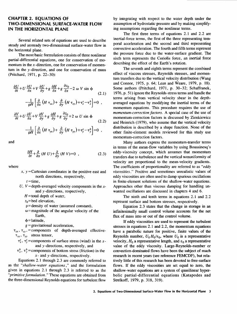
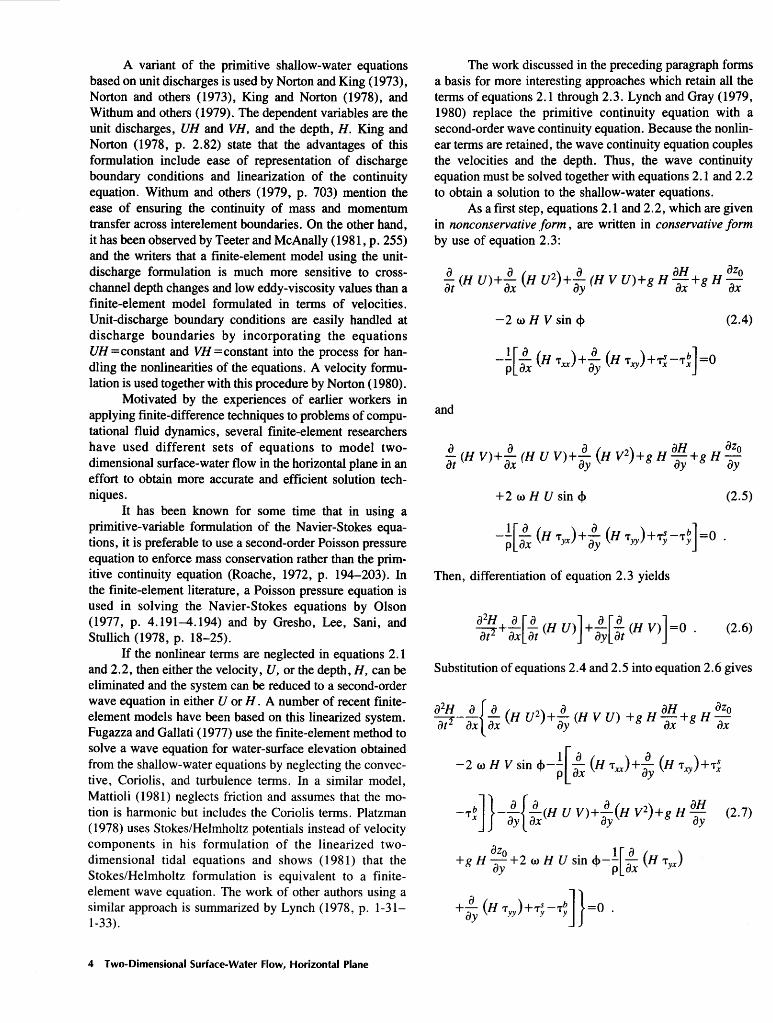
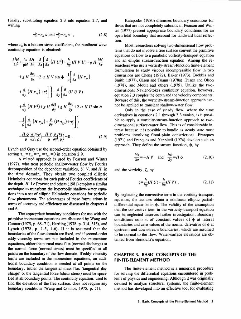

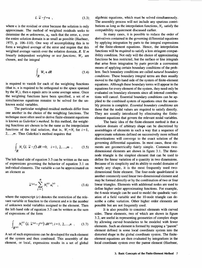

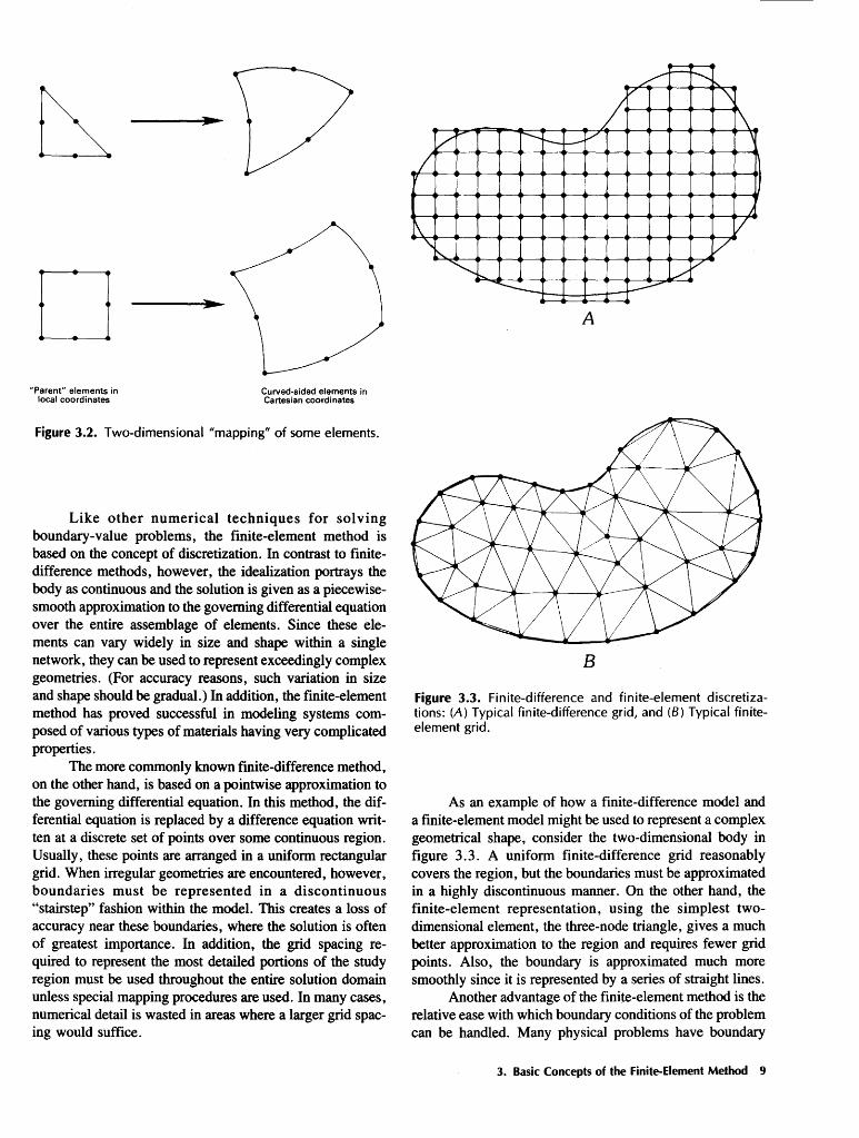

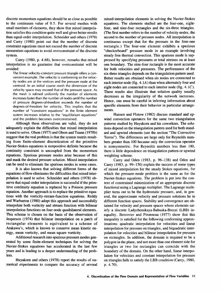
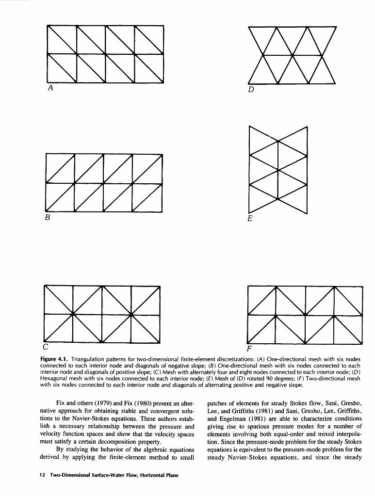

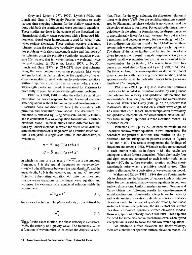


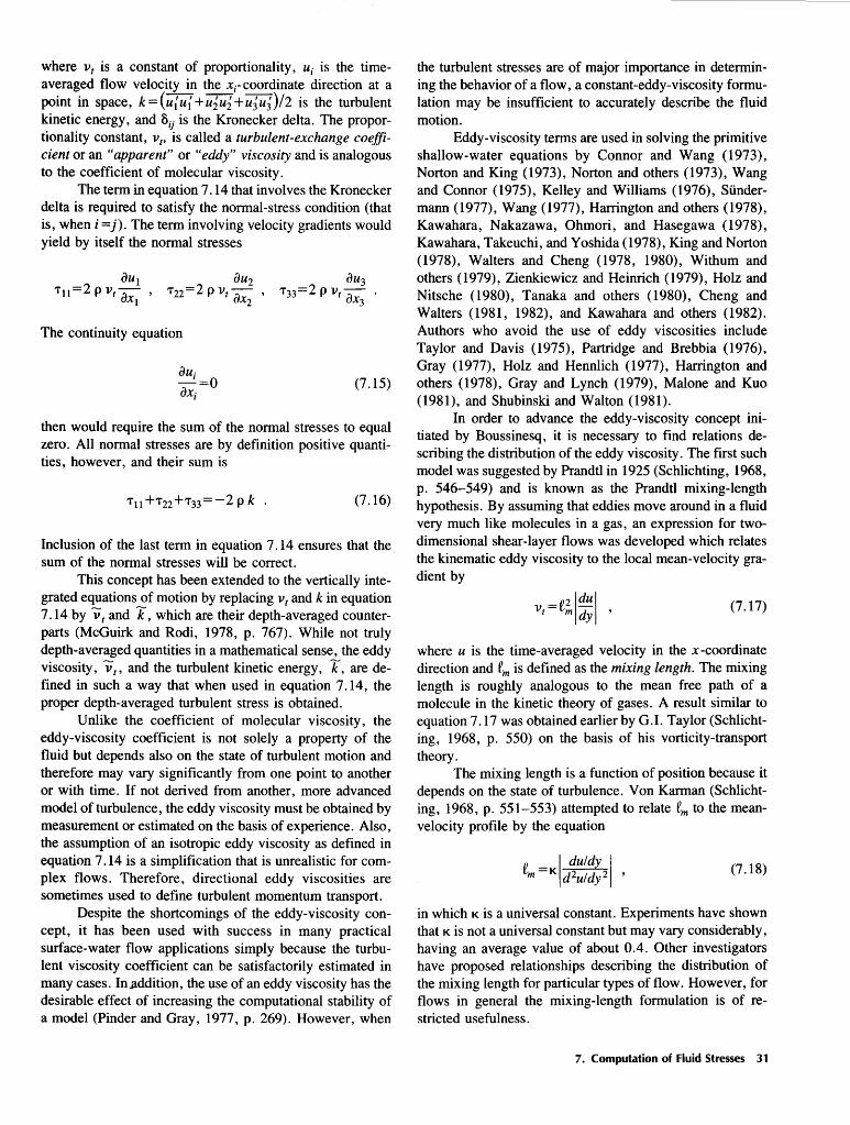
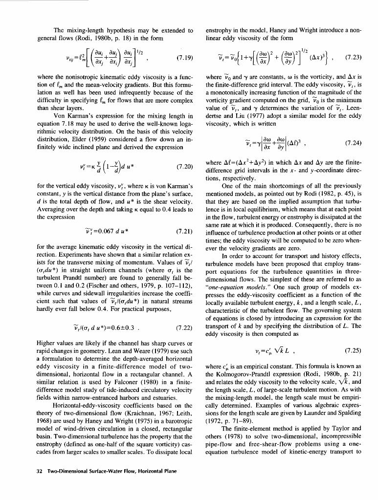

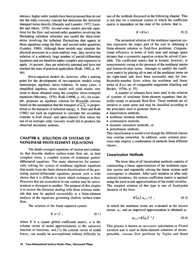


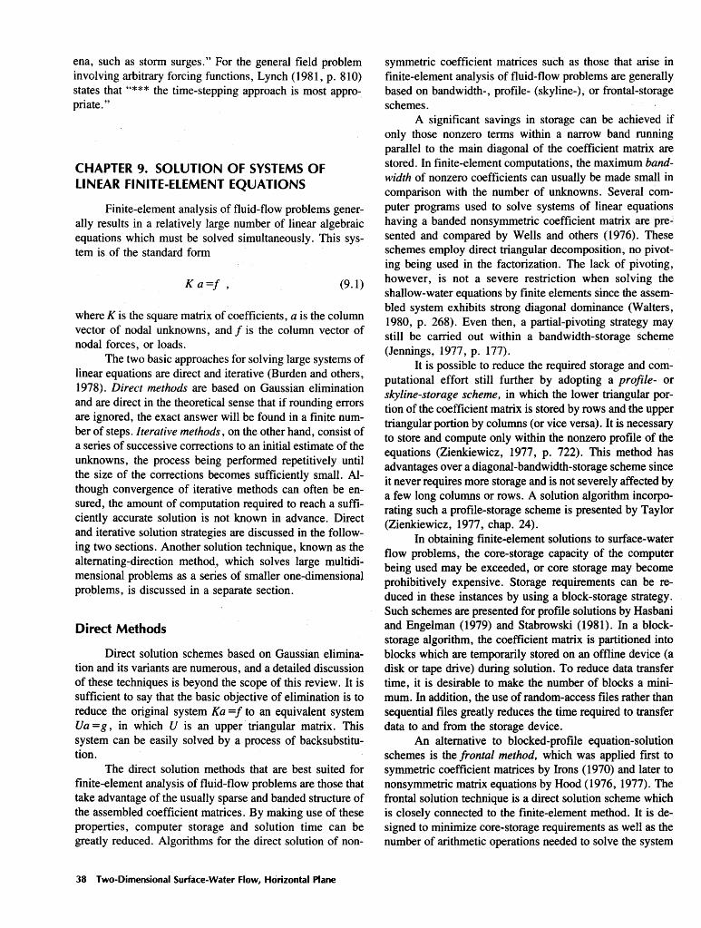
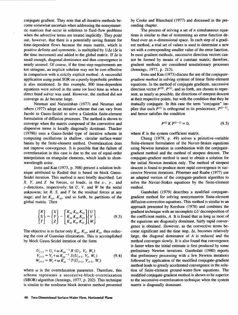


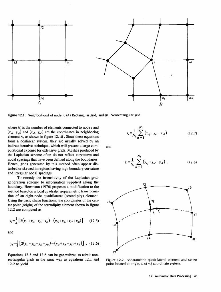
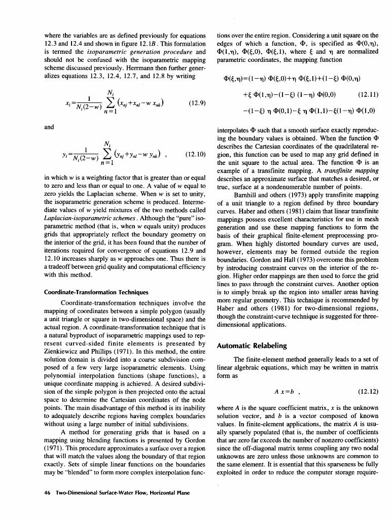


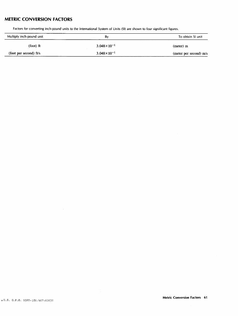


![New finite element algorithm for the coupled · finite element method and the finite differences solutions of the 2D problem is investigated in [4]. Romanian Journal of Physics 63,](https://static.documents.pub/doc/80x56/5e8817d8b98a9c120a0bb942/new-finite-element-algorithm-for-the-finite-element-method-and-the-finite-differences.jpg)


