Review of Preconditioning Methods for FluidDynamics

Abstract

We consider the use of preconditioning methods to accelerate the conver-gence to a steady state for both the incompressible and compressible uid dy-namic equations. Most of the analysis relies on the inviscid equations thoughsome applications for viscous ow are considered. The preconditioning canconsist of either a matrix or a di�erential operator acting on the time deriv-atives. Hence, in the steady state the original steady solution is obtained.For �nite di�erence methods the preconditioning can change and improvethe steady state solutions. Several preconditioners previously discussed arereviewed and some new approaches are presented.

y ICASENASA Langley Research Center

Hampton, Va 23665and

School of Mathematical SciencesSackler Faculty of Exact Sciences

Tel-Aviv UniversityTel-Aviv 69978, Israel

1

1 Introduction

Over the past years numerous researchers have tried to solve the steady state incompress-ible equations for both inviscid and viscous ows. This also lead to attempts to solve thecompressible equations over a large range of mach numbers. A standard way of solvingthe steady state equations is to march the time dependent equations until a steady stateis reached. Since the transient is not of any interest one can use acceleration techniqueswhich destroy the time accuracy but enable one to reach the steady state faster. For theincompresible equations the continuity equation does not contain any time derivatives.To overcome this di�culty Chorin [14] added an arti�cial time derivative of the pressureto the continuity equation together with a multiplicative variable, �. With this arti�-cial term the resultant scheme is a symmetric hyperbolic system for the inviscid terms.Thus, the system is well posed and and numerical method for hyperbolic systems canbe used to advance this system in time.. The free parameter � is then chosen to reachthe steady state quickly. Later Turkel [54] extended this concept by adding the pressuretime derivative to the momentum equations and introducing a second free parameter �.This system can then be analyzed for optimal �, �. The resulting system after precon-ditioning is no longer symmetric but can be symmetrized by a change of variables. Thiswill be shown in more detail later.It is well known that it is di�cult to solve the compressible equations for low Mach

numbers. For an explicit scheme this is easily seen by looking at the time steps. Forstability the time step must be chosen inversely proportional to the largest eigenvalue ofthe system which is approximately the speed of sound, c, for slow ows. However, otherwaves are convected at the uid speed, u , which is much slower. Hence, these wavesdon't change very much over a time step. Thus, thousands of time steps are requiredto reach a steady state. Should one try a multigrid acceleration one �nds that the samedisparity in wave speeds slows down the multigrid acceleration. With an implicit methodan ADI factorization is usually used so that one can easily invert the implicit factors.The use of ADI introduces factorization errors which again slows down the convergencerate when there are wave speeds of very di�erent magnitudes [49] .For small Mach numbers it can be shown ([28], [31] ) that the incompressible equations

approximate the compressible equations. Hence, one needs to justify the use of thecompressible equations for low Mach ows. We present several reasons one would stilluse the compressible equations even though the Mach number of the ow is small.

� There are many sophisticated compressible codes available that could be used forsuch problems especially in complicated geometries

� For low speed aerodynamic problems at high angle of attack most of the of the ow consists of a low Mach number ow. However, there are localized regionscontaining shocks.

� In many problems thermal e�ects are important and the energy equation is coupledto the other equations.

Therefore, one wants to change the transient nature of the system to remove thisdisparity of the wave speeds. Based on an analogy with conjugate gradient methodssuch methods were called [54] preconditioned methods since the object is to reduce thecondition number of the matrix. Another approach, in one dimension, is to diagonalize

the matrix of the inviscid term. One can then use a di�erent time step for each equation,or wave. Upon returning to the original variables one �nds that this is equivalent tomultiplying the time derivatives by a matrix. Hence, this same approach is namedcharacteristic time stepping in [55]. In multidimensions one can no longer completelydecouple the waves by diagonalizing both the entropy and the shear waves and so thecharacteristic time stepping is only an approximation.Thus, for both the incompressible and compressible equations we will consider sys-

tems of the form

wt + fx + gy = 0;(1)

This system is written in conservation form though for some applications this is notnecessary. Our analysis will be based on the linearized equations so that the conservationform does not appear in the analysis though it does appear in the numerical system. Thissystem is now replaced by

P�1wt + fx + gy = 0;(2)

or in linearized form

P�1wt + Awx +Bwy = 0;(3)

In order for this system to be equivalent to the original system in the steady statewe demand that P have an inverse. This only need be true in the ow regime underconsideration. We shall see later that frequently P is singular at stagnation points andalso along the sonic line. Thus, we will only consider strictly subsonic ow without astagnation point or else strictly supersonic ow. For transonic ow it is necessary tosmooth out the singularity in a neighborhood of the sonic line. We also assume that theJacobian matrices A = @f

@wand B = @g

@ware simultaneously symmetrizable. In terms of

the `symmetrizing' variables we also demand that P be positive de�nite. We shall showlater in detail that it does not matter which set of dependent variables are used to developthe preconditioner. One can transform between any two sets of variables. The choiceof variables is dictated only by convenience in constructing the preconditioner. Popularchoices are two out of density, pressure, enthalpy, entropy or temperature in addition tothe velocity components. Thus, when we are �nished we will analyze a system which issimilar to (3) where the matrices A and B are symmetric and P is both symmetric andpositive de�nite. Such systems are known as symmetric hyperbolic systems. One canthen multiply this system by w and integrate by parts to get estimates for the integral ofw2t , i.e. energy estimates. These estimates can then be used to show that the system iswell posed. We stress that if P is not positive then we change the physics of the problem.For example, if P = �I then we have reversed the time direction and must thereforechange all the bounday conditions. Hence, to be sure that the system is well posed withthe original type of boundary conditions we shall only consider the symmetric hyperbolicsystem. For more general systems one must use a more complicated analysis to showwell-posedness for the initial-boundary value problem ([30], [63]).With these assumptions we see that the steady state solutions of the two systems

are the same. Assuming the steady state has a unique solution it does not matter whichsystem we march to a steady state. We shall later see that for the �nite di�erence

approximations the steady state solutions are not the necessarily same and usually thepreconditioned system leads to a better behaved steady state.We can also look at (3) from a di�erent viewpoint. We assume that the matrices A

and B are symmetric and P is positive de�nite. It is well known that for the Euler equa-tions that the matrices A and B cannot be simultaneously diagonalized by a similaritytransformation. However, the matrix P has changed the equation. Since P is positivede�nite there exists a matrix Q so that P = QQ?. We then introduce a new variablew = Qv. For constant coe�cients A, B (3) is replaced by

vt +Q?AQvx +Q

?BQvy = 0;(4)

Thus, the diagonalization question changes and we wish to know if A and B canbe simultaneously diagonalized by a congruence transformation (Q?AQ) . A su�cientcondition for this to be true is that there exist numbers !1; !2 so that !1A + !2B ispositive de�nite. It is shown in [53] that this true for supersonic ow. Hence, we haveshown that for supersonic ow one can introduce a preconditioning matrix so that theequations (constant coe�cients) are diagonalized. However, this is not true for subsonic ow. We shall later show that using di�erential operators one can diagonalize the systemeven for subsonic ow.

2 Incompressible equations

We �rst consider the incompressible inviscid equations in primitive variables.

ux + vy = 0

ut + uux + vuy + px = 0(5)

vt + uvx + vvy + py = 0

We consider generalizations of Chorin's pseudo-compressibility method [14]. Using thepreconditioning suggested in [54] we have

1

�2pt + ux + vy = 0

�u

�2pt + ut + uux + vuy + px = 0(6)

�v

�2pt + vt + uvx + vvy + py = 0

or in conservation form

1

�2pt + ux + vy = 0

(�+ 1)u

�2pt + ut + (u

2 + p)x + (uv)y = 0(7)

(�+ 1)v

�2pt + vt + (uv)x + (v

2 + p)y = 0

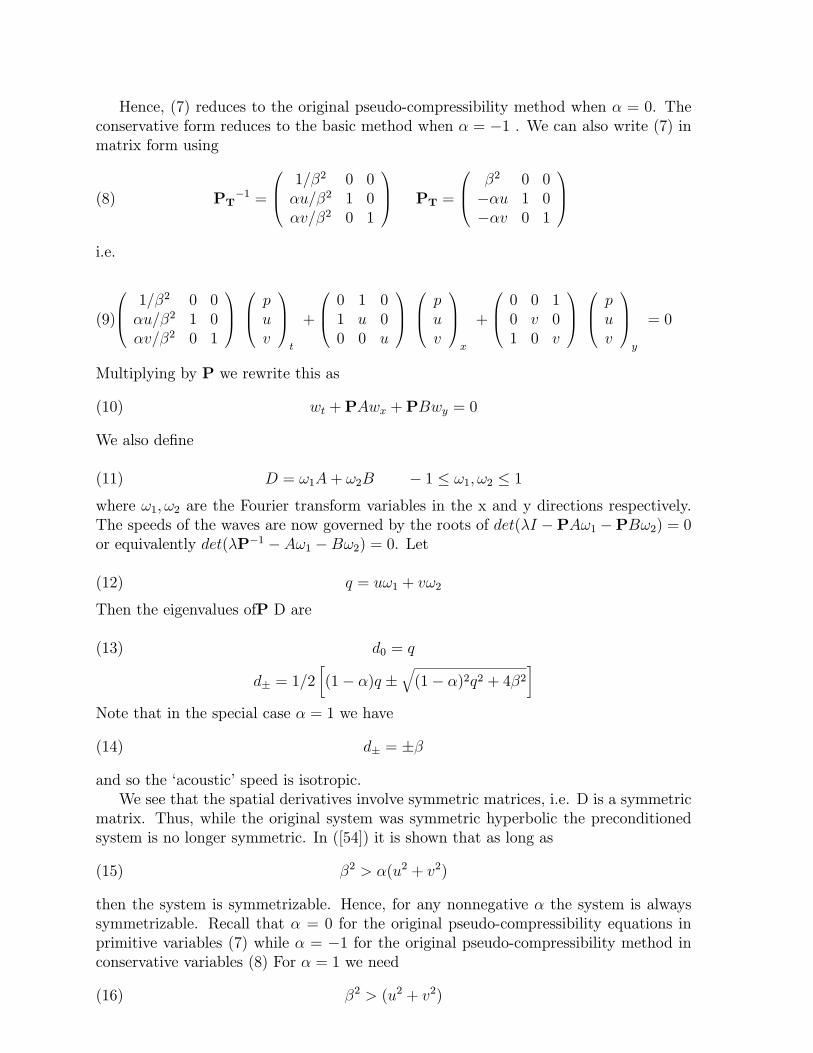
Hence, (7) reduces to the original pseudo-compressibility method when � = 0. Theconservative form reduces to the basic method when � = �1 . We can also write (7) inmatrix form using

PT�1 =

0B@ 1=�2 0 0�u=�2 1 0�v=�2 0 1

1CA PT =

0B@ �2 0 0��u 1 0��v 0 1

1CA(8)

i.e.

0B@ 1=�2 0 0�u=�2 1 0�v=�2 0 1

1CA0B@ puv

1CAt

+

0B@ 0 1 01 u 00 0 u

1CA0B@ puv

1CAx

+

0B@ 0 0 10 v 01 0 v

1CA0B@ puv

1CAy

= 0(9)

Multiplying by P we rewrite this as

wt +PAwx +PBwy = 0(10)

We also de�ne

D = !1A+ !2B � 1 � !1; !2 � 1(11)

where !1; !2 are the Fourier transform variables in the x and y directions respectively.The speeds of the waves are now governed by the roots of det(�I �PA!1 �PB!2) = 0or equivalently det(�P�1 � A!1 �B!2) = 0. Let

q = u!1 + v!2(12)

Then the eigenvalues ofP D are

d0 = q(13)

d� = 1=2�(1� �)q �

q(1� �)2q2 + 4�2

�Note that in the special case � = 1 we have

d� = ��(14)

and so the `acoustic' speed is isotropic.We see that the spatial derivatives involve symmetric matrices, i.e. D is a symmetric

matrix. Thus, while the original system was symmetric hyperbolic the preconditionedsystem is no longer symmetric. In ([54]) it is shown that as long as

�2 > �(u2 + v2)(15)

then the system is symmetrizable. Hence, for any nonnegative � the system is alwayssymmetrizable. Recall that � = 0 for the original pseudo-compressibility equations inprimitive variables (7) while � = �1 for the original pseudo-compressibility method inconservative variables (8) For � = 1 we need

�2 > (u2 + v2)(16)

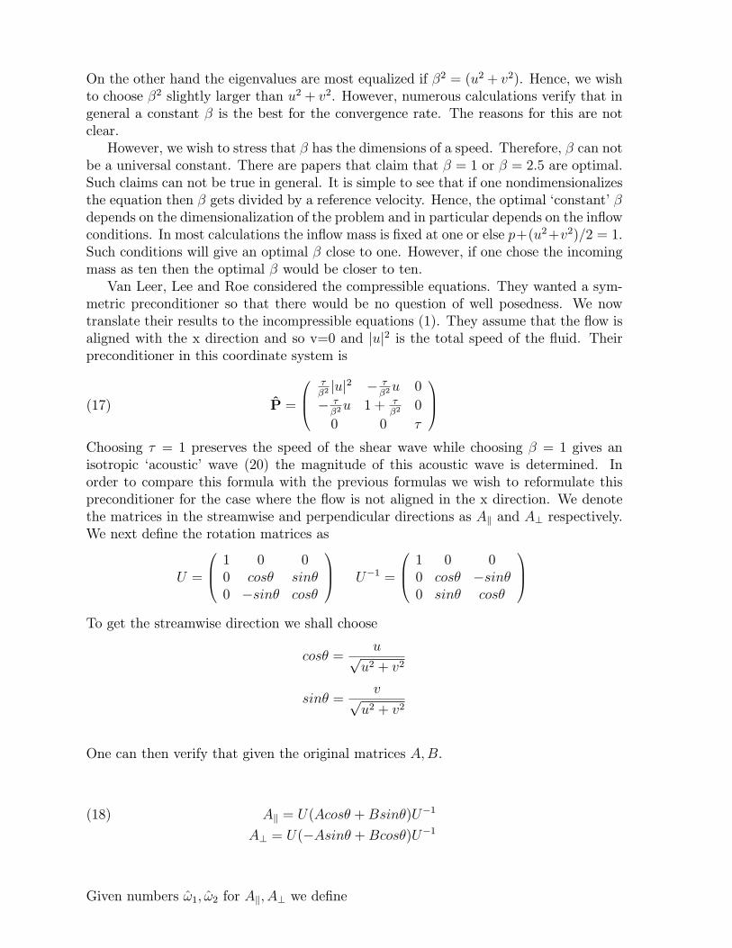
On the other hand the eigenvalues are most equalized if �2 = (u2 + v2). Hence, we wishto choose �2 slightly larger than u2 + v2. However, numerous calculations verify that ingeneral a constant � is the best for the convergence rate. The reasons for this are notclear.However, we wish to stress that � has the dimensions of a speed. Therefore, � can not

be a universal constant. There are papers that claim that � = 1 or � = 2:5 are optimal.Such claims can not be true in general. It is simple to see that if one nondimensionalizesthe equation then � gets divided by a reference velocity. Hence, the optimal `constant' �depends on the dimensionalization of the problem and in particular depends on the in owconditions. In most calculations the in ow mass is �xed at one or else p+(u2+v2)=2 = 1.Such conditions will give an optimal � close to one. However, if one chose the incomingmass as ten then the optimal � would be closer to ten.Van Leer, Lee and Roe considered the compressible equations. They wanted a sym-

metric preconditioner so that there would be no question of well posedness. We nowtranslate their results to the incompressible equations (1). They assume that the ow isaligned with the x direction and so v=0 and juj2 is the total speed of the uid. Theirpreconditioner in this coordinate system is

P =

0B@��2juj2 � �

�2u 0

� ��2u 1 + �

�20

0 0 �

1CA(17)

Choosing � = 1 preserves the speed of the shear wave while choosing � = 1 gives anisotropic `acoustic' wave (20) the magnitude of this acoustic wave is determined. Inorder to compare this formula with the previous formulas we wish to reformulate thispreconditioner for the case where the ow is not aligned in the x direction. We denotethe matrices in the streamwise and perpendicular directions as Ak and A? respectively.We next de�ne the rotation matrices as

U =

0B@ 1 0 00 cos� sin�0 �sin� cos�

1CA U�1 =

0B@ 1 0 00 cos� �sin�0 sin� cos�

1CATo get the streamwise direction we shall choose

cos� =up

u2 + v2

sin� =vp

u2 + v2

One can then verify that given the original matrices A;B.

Ak = U(Acos� +Bsin�)U�1(18)

A? = U(�Asin� +Bcos�)U�1

Given numbers !1; !2 for Ak; A? we de�ne

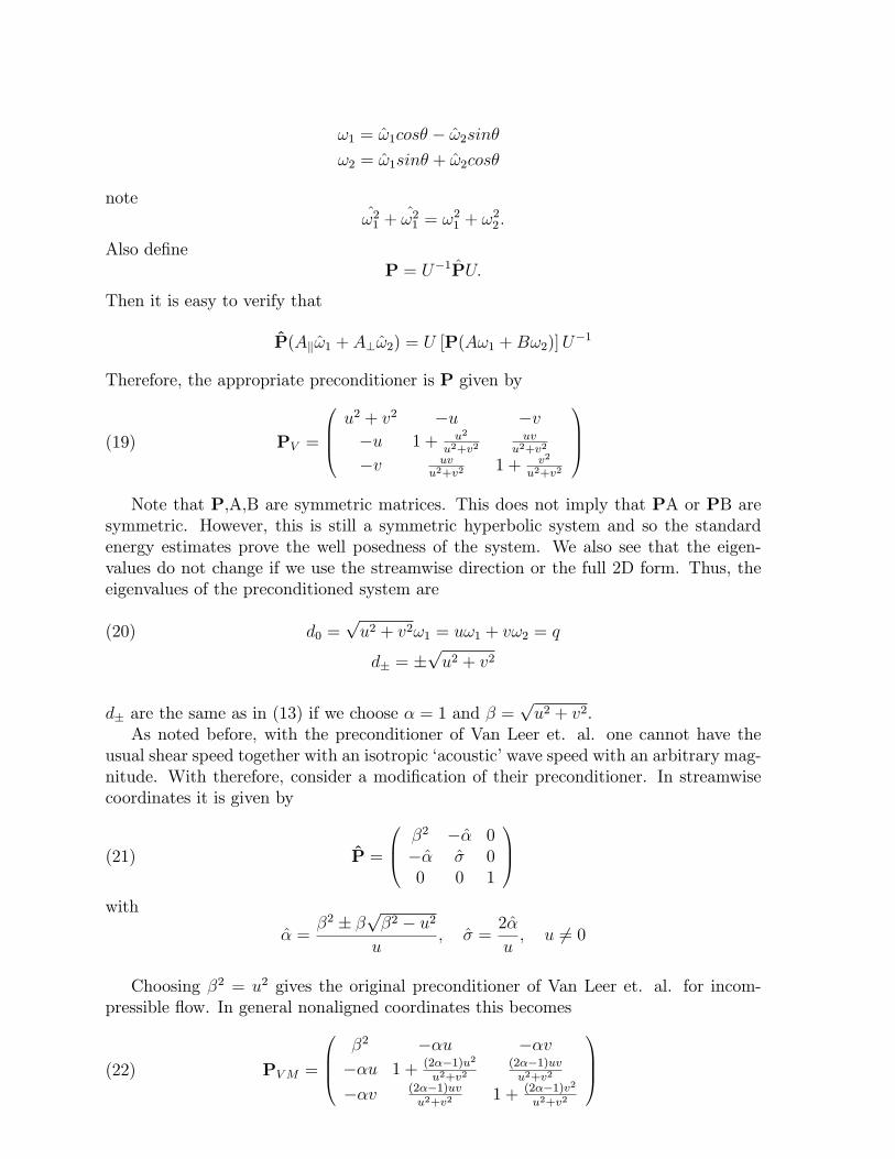
!1 = !1cos� � !2sin�!2 = !1sin� + !2cos�

note!21 + !

21 = !

21 + !

22:

Also de�neP = U�1PU:

Then it is easy to verify that

P(Ak!1 + A?!2) = U [P(A!1 +B!2)]U�1

Therefore, the appropriate preconditioner is P given by

PV =

0BB@u2 + v2 �u �v�u 1 + u2

u2+v2uv

u2+v2

�v uvu2+v2

1 + v2

u2+v2

1CCA(19)

Note that P,A,B are symmetric matrices. This does not imply that PA or PB aresymmetric. However, this is still a symmetric hyperbolic system and so the standardenergy estimates prove the well posedness of the system. We also see that the eigen-values do not change if we use the streamwise direction or the full 2D form. Thus, theeigenvalues of the preconditioned system are

d0 =pu2 + v2!1 = u!1 + v!2 = q(20)

d� = �pu2 + v2

d� are the same as in (13) if we choose � = 1 and � =pu2 + v2.

As noted before, with the preconditioner of Van Leer et. al. one cannot have theusual shear speed together with an isotropic `acoustic' wave speed with an arbitrary mag-nitude. With therefore, consider a modi�cation of their preconditioner. In streamwisecoordinates it is given by

P =

0B@ �2 �� 0�� � 00 0 1

1CA(21)

with

� =�2 � �

p�2 � u2u

; � =2�

u; u 6= 0

Choosing �2 = u2 gives the original preconditioner of Van Leer et. al. for incom-pressible ow. In general nonaligned coordinates this becomes

PVM =

0BB@�2 ��u ��v��u 1 + (2��1)u2

u2+v2(2��1)uvu2+v2

��v (2��1)uvu2+v2

1 + (2��1)v2u2+v2

1CCA(22)

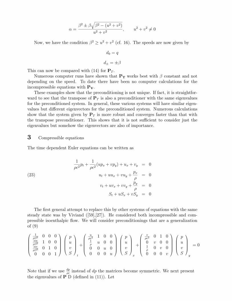
� =�2 � �

q�2 � (u2 + v2)u2 + v2

; u2 + v2 6= 0

Now, we have the condition �2 � u2 + v2 (cf. 16). The speeds are now given by

d0 = q

d� = ��This can now be compared with (14) for PT .Numerous computer runs have shown that PT works best with � constant and not

depending on the speed. To date there have been no computer calculations for theincompressible equations with PV.These examples show that the preconditioning is not unique. If fact, it is straightfor-

ward to see that the transpose of PT is also a preconditioner with the same eigenvaluesfor the preconditioned system. In general, these various systems will have similar eigen-values but di�erent eigenvectors for the preconditioned system. Numerous calculationsshow that the system given by PT is more robust and converges faster than that withthe transpose preconditioner. This shows that it is not su�cient to consider just theeigenvalues but somehow the eigenvectors are also of importance.

3 Compressible equations

The time dependent Euler equations can be written as

1

�c2pt +

1

�c2(upx + vpy) + ux + vy = 0

ut + uux + vuy +px�

= 0(23)

vt + uvx + vvy +py�

= 0

St + uSx + vSy = 0

The �rst general attempt to replace this by other systems of equations with the samesteady state was by Viviand ([59],[27]). He considered both incompressible and com-pressible isoenthalpic ow. We will consider preconditionings that are a generalizationof (9)0BBBB@

1��2

0 0 0�u��2

1 0 0�v��2

0 1 0

0 0 0 1

1CCCCA0BBB@puvS

1CCCAt

+

0BBBB@u�c2

1 0 01�

u 0 0

0 0 u 00 0 0 u

1CCCCA0BBB@puvS

1CCCAx

+

0BBBB@v�c2

0 1 0

0 v 0 01�

0 v 0

0 0 0 v

1CCCCA0BBB@puvS

1CCCAy

= 0

Note that if we use dp�cinstead of dp the matrices become symmetric. We next present

the eigenvalues of P D (de�ned in (11)). Let

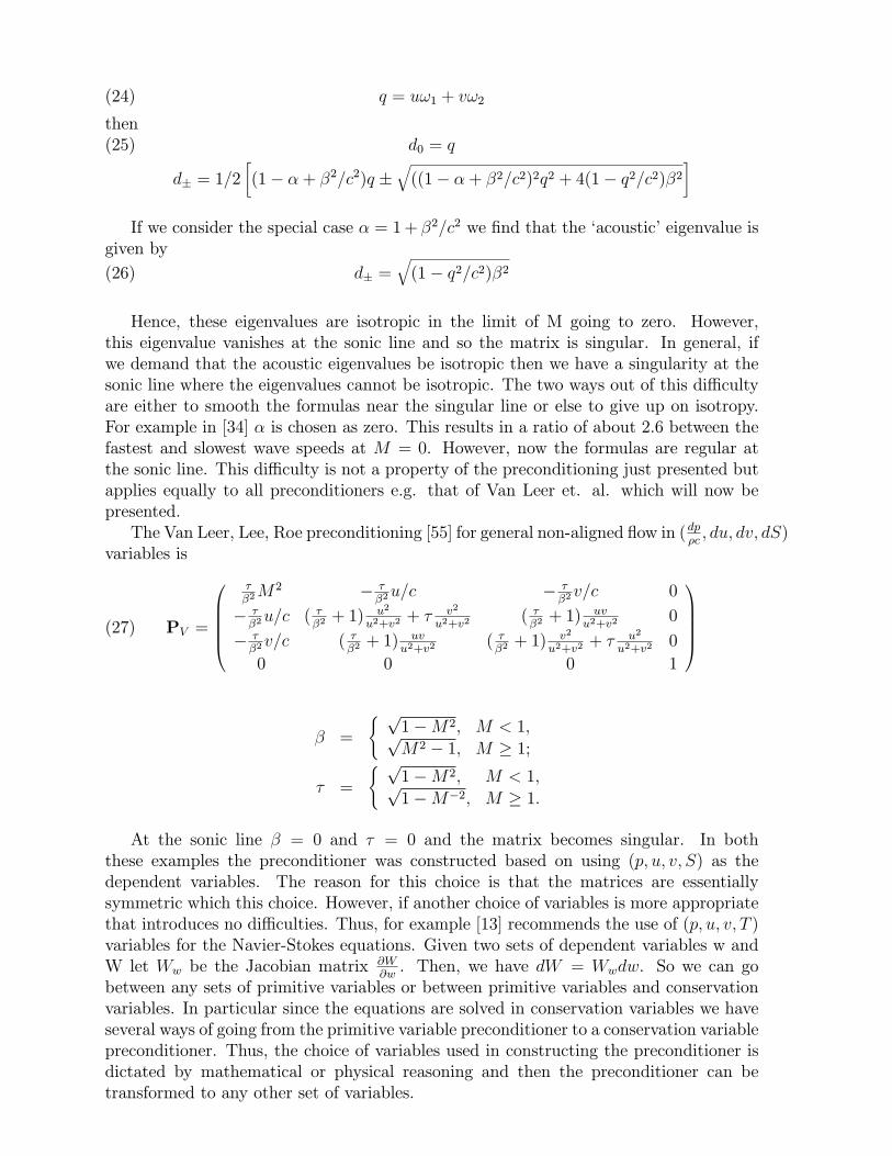
q = u!1 + v!2(24)

thend0 = q(25)

d� = 1=2�(1� �+ �2=c2)q �

q((1� �+ �2=c2)2q2 + 4(1� q2=c2)�2

�

If we consider the special case � = 1+ �2=c2 we �nd that the `acoustic' eigenvalue isgiven by

d� =q(1� q2=c2)�2(26)

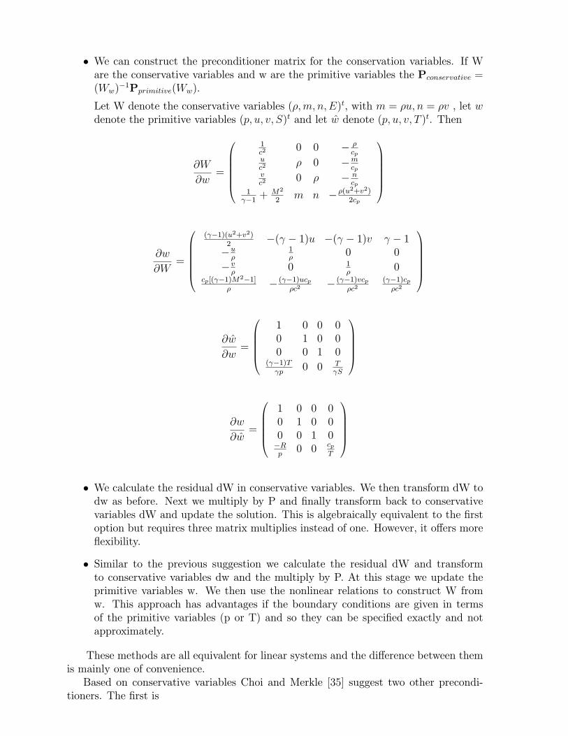
Hence, these eigenvalues are isotropic in the limit of M going to zero. However,this eigenvalue vanishes at the sonic line and so the matrix is singular. In general, ifwe demand that the acoustic eigenvalues be isotropic then we have a singularity at thesonic line where the eigenvalues cannot be isotropic. The two ways out of this di�cultyare either to smooth the formulas near the singular line or else to give up on isotropy.For example in [34] � is chosen as zero. This results in a ratio of about 2.6 between thefastest and slowest wave speeds at M = 0. However, now the formulas are regular atthe sonic line. This di�culty is not a property of the preconditioning just presented butapplies equally to all preconditioners e.g. that of Van Leer et. al. which will now bepresented.The Van Leer, Lee, Roe preconditioning [55] for general non-aligned ow in (dp

�c; du; dv; dS)

variables is

PV =

0BBBB@��2M2 � �

�2u=c � �

�2v=c 0

� ��2u=c ( �

�2+ 1) u2

u2+v2+ � v2

u2+v2( ��2+ 1) uv

u2+v20

� ��2v=c ( �

�2+ 1) uv

u2+v2( ��2+ 1) v2

u2+v2+ � u2

u2+v20

0 0 0 1

1CCCCA(27)

� =

( p1�M2; M < 1;pM2 � 1; M � 1;

� =

( p1�M2; M < 1;p1�M�2; M � 1:

At the sonic line � = 0 and � = 0 and the matrix becomes singular. In boththese examples the preconditioner was constructed based on using (p; u; v; S) as thedependent variables. The reason for this choice is that the matrices are essentiallysymmetric which this choice. However, if another choice of variables is more appropriatethat introduces no di�culties. Thus, for example [13] recommends the use of (p; u; v; T )variables for the Navier-Stokes equations. Given two sets of dependent variables w andW let Ww be the Jacobian matrix

@W@w. Then, we have dW = Wwdw. So we can go

between any sets of primitive variables or between primitive variables and conservationvariables. In particular since the equations are solved in conservation variables we haveseveral ways of going from the primitive variable preconditioner to a conservation variablepreconditioner. Thus, the choice of variables used in constructing the preconditioner isdictated by mathematical or physical reasoning and then the preconditioner can betransformed to any other set of variables.

� We can construct the preconditioner matrix for the conservation variables. If Ware the conservative variables and w are the primitive variables the Pconservative =(Ww)

�1Pprimitive(Ww).

Let W denote the conservative variables (�;m; n;E)t, with m = �u; n = �v , let wdenote the primitive variables (p; u; v; S)t and let w denote (p; u; v; T )t. Then

@W

@w=

0BBBBB@1c2

0 0 � �cp

uc2

� 0 �mcp

vc2

0 � � ncp

1 �1 +

M2

2m n ��(u2+v2)

2cp

1CCCCCA

@w

@W=

0BBBBB@( �1)(u2+v2)

2�( � 1)u �( � 1)v � 1

�u�

1�

0 0

�v�

0 1�

0cp[( �1)M2�1]

�� ( �1)ucp

�c2� ( �1)vcp

�c2( �1)cp�c2

1CCCCCA

@w

@w=

0BBBB@1 0 0 00 1 0 00 0 1 0

( �1)T p

0 0 T S

1CCCCA

@w

@w=

0BBBB@1 0 0 00 1 0 00 0 1 0�Rp

0 0 cpT

1CCCCA

� We calculate the residual dW in conservative variables. We then transform dW todw as before. Next we multiply by P and �nally transform back to conservativevariables dW and update the solution. This is algebraically equivalent to the �rstoption but requires three matrix multiplies instead of one. However, it o�ers more exibility.

� Similar to the previous suggestion we calculate the residual dW and transformto conservative variables dw and the multiply by P. At this stage we update theprimitive variables w. We then use the nonlinear relations to construct W fromw. This approach has advantages if the boundary conditions are given in termsof the primitive variables (p or T) and so they can be speci�ed exactly and notapproximately.

These methods are all equivalent for linear systems and the di�erence between themis mainly one of convenience.Based on conservative variables Choi and Merkle [35] suggest two other precondi-

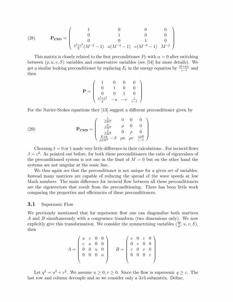
tioners. The �rst is

PCM1 =

0BBBB@1 0 0 00 1 0 00 0 1 0

u2+v2

2(M�2 � 1) u(M�2 � 1) v(M�2 � 1) M�2

1CCCCA(28)

This matrix is closely related to the �rst preconditioner PT with � = 0 after switchingbetween (p; u; v; S) variables and conservative variables (see [54] for more details). We

get a similar looking preconditioner by replacing Et in the energy equation by(E+p)t �1 and

then

P =

0BBBB@1 0 0 00 1 0 00 0 1 0

u2+v2

2�u �v

�1

1CCCCAFor the Navier-Stokes equations they [13] suggest a di�erent preconditioner given by

PCM2 =

0BBBB@1

�M2 0 0 0u

�M2 � 0 0v

�M2 0 � 0E+p��M2 � � �u �v �R

�1

1CCCCA(29)

Choosing � = 0 or 1 made very little di�erence in their calculations.. For inviscid ows� = c2. As pointed out before, for both these preconditioners the ratio of eigenvalues ofthe preconditioned system is not one in the limit of M = 0 but on the other hand thesystems are not singular at the sonic line.We thus again see that the preconditioner is not unique for a given set of variables.

Instead many matrices are capable of reducing the spread of the wave speeds at lowMach numbers. The main di�erence for inviscid ow between all these preconditionersare the eigenvectors that result from the preconditioning. There has been little workcomparing the properties and e�ciencies of these preconditioners.

3.1 Supersonic Flow

We previously mentioned that for supersonic ow one can diagonalize both marticesA and B simultaneously with a congruence transform (two dimensions only). We nowexplicitly give this transformation. We consider the symmetrizing variables (dp

�c; u; v; S),

then

A =

0BBBBBB@u c 0 0c u 0 00 0 u 00 0 0 u

1CCCCCCA B =

0BBBBBB@v 0 c 00 v 0 0c 0 v 00 0 0 v

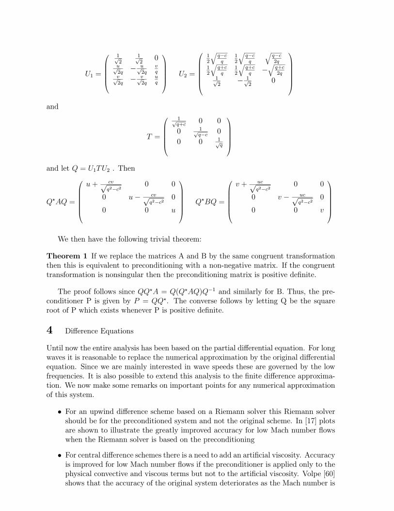
1CCCCCCALet q2 = u2 + v2. We assume u � 0; v � 0. Since the ow is supersonic q � c. The

last row and column decouple and so we consider only a 3x3 submatrix. De�ne,

U1 =

0BBBB@1p2

1p2

0up2q

� up2q

vq

vp2q

� vp2q

uq

1CCCCA U2 =

0BBBBB@12

qq�cq

12

qq�cq

qq�c2q

12

qq+cq

12

qq+cq

�qq+c2q

1p2

� 1p2

0

1CCCCCAand

T =

0BBBB@1pq+c

0 0

0 1pq�c 0

0 0 1pq

1CCCCAand let Q = U1TU2 . Then

Q?AQ =

0BBBBB@u+ cvp

q2�c20 0

0 u� cvpq2�c2

0

0 0 u

1CCCCCA Q?BQ =

0BBBBB@v + ucp

q2�c20 0

0 v � ucpq2�c2

0

0 0 v

1CCCCCAWe then have the following trivial theorem:

Theorem 1 If we replace the matrices A and B by the same congruent transformationthen this is equivalent to preconditioning with a non-negative matrix. If the congruenttransformation is nonsingular then the preconditioning matrix is positive de�nite.

The proof follows since QQ?A = Q(Q?AQ)Q�1 and similarly for B. Thus, the pre-conditioner P is given by P = QQ?. The converse follows by letting Q be the squareroot of P which exists whenever P is positive de�nite.

4 Di�erence Equations

Until now the entire analysis has been based on the partial di�erential equation. For longwaves it is reasonable to replace the numerical approximation by the original di�erentialequation. Since we are mainly interested in wave speeds these are governed by the lowfrequencies. It is also possible to extend this analysis to the �nite di�erence approxima-tion. We now make some remarks on important points for any numerical approximationof this system.

� For an upwind di�erence scheme based on a Riemann solver this Riemann solvershould be for the preconditioned system and not the original scheme. In [17] plotsare shown to illustrate the greatly improved accuracy for low Mach number owswhen the Riemann solver is based on the preconditioning

� For central di�erence schemes there is a need to add an arti�cial viscosity. Accuracyis improved for low Mach number ows if the preconditioner is applied only to thephysical convective and viscous terms but not to the arti�cial viscosity. Volpe [60]shows that the accuracy of the original system deteriorates as the Mach number is

reduced. The author has had a similar experience in three dimensional ows arounda fuselage con�guration. The use of a matrix arti�cial dissipation ([51]) should bebased on the preconditioned equations as in the upwind di�erence scheme. On theother hand Merkle (private communication) has indicated that he has no di�cultieswith accuracy in the very low Mach regime. He can take the solution obtained witha preconditioner and use that as initial data for a nonpreconditioned code whichthen simply converges in one time step with the same small residual. In thiscase both the original system and the preconditioned system give the same resultseven on the di�erence level. Upwind schemes tend to have more di�culties withaccuracy for low Mach ows [17].

Hence, both for upwind and central di�erence schemes the Riemann solver orarti�cial viscosity should be based on P�1jPAj and not jAj. i.e. in one dimensionsolve wt + Pfx = (jPAjwx)x . For a scalar arti�cial viscosity jPAj is replacedby the spectral radius of P A or equivalently the time step associated with thepreconditioned matrix. This is equivalent to not multiplying the arti�cial viscosityby P.

� Similarly, when using characteristics in the boundary conditions these should bebased on the characteristics of the modi�ed system and not the physical system.

� When using multigrid it is better to transfer the residuals based on the precondi-tioned system to the next grid since these residuals are more balanced than thephysical residuals.

Preconditioning is even more important when using multigrid than with an explicitscheme. With the original system the disparity of the eigenvalues greatly a�ects thesmoothing rates of the slow components and so slows down the multigrid method,[56].

� In addition to convergence di�culties there are accuracy di�culies at low Machnumbers [60]. Some of these can be alleviated by preconditioning the dissipationterms as indicated above. For very small Mach numbers there is also a di�cultywith roundo� errors as p

u2+v2! 1. Several people have suggested subtracting

out a constant pressure from the dynamic pressure. A more detailed analysis [20]suggests replacing the pressure p by ~p where p = p0+�~p

�2and � is a representative

Mach number.

� We conclude from the above remarks that the steady state solution of the precon-ditioned system may be di�erent from that of the physical system. Thus, on the�nite di�erence level the preconditioning can improve the accuracy as well as theconvergence rate.

5 Di�erential Preconditioners

In the previous sections the preconditioner P was a matrix. For the nonlinear uiddynamic equations the elements of P involved the dependent variables. There are severallimitations with this approach.We �rst consider a scalar equation

wt + awx + bwy = 0;(30)

We consider a uniform cartesian mesh with constant �x;�y. We de�ne the aspect ratiofor this problem as

ar = aspect ratio = a=�xb=�y

.

This can be interpreted as the ratio of time for a wave to traverse a mesh in the xdirection relative to the time in the y direction. We note that the ratio �y

�xis meaningless

since this can be changed by a trivial change of variables.If this aspect ratio di�ers greatly from one then the standard schemes will converge

slowly since a time step appropriate for one direction is inappropriate for the otherdirection. For a scalar equation, this is an arti�cial problem since, in practice, the meshwould be chosen so that the aspect ratio is close to one. However, for a system ofequations there are many waves. If the aspect ratio is close to one for one wave it willnot be close to one for other waves. In the boundary layer for the acoustic wave ar =(u+c)=�x(v+c)=�y

� �y�x. However, for the shear wave ar � u

v�y�xand away from the wall but in

the boundary layer u is much larger than v. Hence, any mesh that is appropriate forthe acoustic wave is not appropriate for the shear and entropy waves and vice versa. Inaddition there are viscous e�ects that we are ignoring, so that in practice the mesh isconstructed based on viscous e�ects and ignores both the acoustic and entropy waves.For the scalar equation we are considering algebraic preconditioning cannot help (Liand Van Leer, private communication). For a system the preconditionings we haveconsidered can partially rectify the di�erence of speeds between the various waves butdoes not alleviate the aspect ratio di�culty.The matrix preconditioners we have considered until now have a second di�culty.

For one dimensional ow one can choose the preconditioner as the absolute value of thematrix A. Then all the resultant waves have identical speeds with only di�erences inthe direction, positive or negative. However, in two space dimension when the matricesA and B do not commute it is not possible, in general , to equalize all the speeds.Equivalently, we cannot diagonalize the system and reduce it to a sequence of scalarequations even for the frozen coe�cient problem.To alleviate these two problems we shall allow the preconditioner P to contain deriv-

atives. However, as before we still demand that for the symmetric equations that P beinvertible and be positive de�nite.For the scalar equation (30) we consider a preconditioner based on residual smoothing

[26]. This is given by

(1� �x@xx)(1� �y@yy)Resnew = Resold(31)

where Res refers to the residual before and after smoothing. This residual smoothingis usually introduced to improve the time step and smoothing properties of an explicitscheme as Runge-Kutta or Lax-Wendro�. Here, we analyze the scheme from a di�erentperspective, that of wave speeds. We assume that the aspect ration for the problem isvery large (i.e. b is large compared to a or �y is small compared to �x ). The questionwe wish to address is whether �x and �y can be chosen so as to reduce this aspect ratio.We �rst consider residual smoothing in one space dimension. In this case there is

no aspect ratio. Instead we will show how the concept of wave speeds explains thephenomena that one should not use residual smoothing with a very large time step eventhough it can be stabilized by choosing an appropriately large �..

(1� �@xx)wt + awx = 0

We analyze this for a semi-discrete equation with time continuous, the �rst x deriv-ative approximated by a central di�erence and the second space derivative by a threepoint central di�erence. In order to �nd the phase and group velocities we considersolutions of the form w = ei(kx�!t). Here k is given and we �nd ! from the dispersionrelation. For the one dimensional residual smoothing we have

k = asin�; ! =asin�=�x

1 + 2�(1� cos�)

� = k�xTo �nd a stability condition for a Runge-Kutta scheme in time we maximize ! and

�nd that the worst case is cos� = 2�1+2�

. We then �nd that the scheme is stable if

� � 1

4(r2 � 1)

where r = �tnew�toriginal

.Thus, from the viewpoint of stability we can choose any time step

we wish by choosing � su�ciently large. Nevertheless, one �nds computationally thatconvergence to a steady state is slowed down by choosing �t, and hence �, too large.Optimal values are r � 2. We shall now show from the viewpoint of wave propagationthat it is not good to choose a very large time step.Residual smoothing adds a term wxxt to the original di�erential equation. Such a

term is a dispersive term i.e. the energy is not reduced but now the speed of a plane waveis no longer constant but instead depends on the wave number. The main purpose ofthis term is to increase the time stability limit. However, as in de�ning the aspect ratio,increasing the time step is meaningful only if we normalize the solution in some way,otherwise we are merely rescaling the time dimension. Hence, the appropriate quantityis not the time step but rather the time it takes a wave to transverse one cell (assuming�x is constant). The phase speed of a plane wave is given by

vp =!

k=

a

1 + 4�sin2�=2

Let � = 14(r2 � 1) and multiply vp by r to get the distance transversed in time �t.

Then

sp = relative phase distance =2r

(r2 + 1)� (r2 � 1)cos�(32)

For the long wave lengths cos� � 1 and so sp � r, i.e. the long wave lenths mover times further in one time step. If we look at � = �=2, we have sp =

2rr2+1

� 1. Thusthis frequency moves slower than without residual smoothing. For the highest frequencyon the mesh we have � = � and sp =

1r. We therefore, see that the high frequencied

are actually slowed down by the residual smoothing and so take longer to exit fromthe domain, furthermore the larger �t is chosen the slower these waves go. Even moreimportant the larger �t is chosen the more frequencies that are slowed down even thoughthe lowest frequencies travel faster. The breakeven frequency is given by cos� = r�1

r+1.

We can also consider the group velocity. For the optimal � this is given by

vg =d!

dk= 2

(r2 + 1)cos� � (r2 � 1)cos2�[(r2 + 1)� (r2 � 1)cos�]2

and

sg = sp(r2 + 1)cos� � (r2 � 1)cos2�(r2 + 1)� (r2 � 1)cos�(33)

The situation now is even less favorable than before. Again, the lowest frequencies aresped up by a factor r. The frequency � = �=2 is slowed down by an additional factor ofr2�1r2+1

and the highest frequency � = � now reverses direction and goes upstream .In �gures (1a-1c) we plot the phase and group relative distances for r=2,5,10. As

demonstrated above we gain a factor of r for the low fequencies but actually lose comparedwith r=1 for the high frequencies. As r is increased more frequencies get slowed down.Because we are considering the semi-discrete equation and residual smoothing is purelydispersive there is no damping of the waves. For a Runge-Kutta scheme one �nds thatas r is increased that the damping of high frequencies decreases. Thus, for large r thehigh frequencies do not propagate very fast and are not damped either. This explainsone in practice one chooses an r of about two for the greatest increase in the convergencerate to a steady state.We next consider the two dimensional equation. To ease the derivations we shall con-

sider the partial di�erential equation (31) rather than the �nite di�erence approximation.We rewrite (31) as

ut � �xuxxt � �yuyyt + �x�yuxxyyt = aux + buy(34)

We are interested in the e�ect of high aspect ratios. So we consider �y << �x . Byrescaling we instead consider a uniform mesh but a << b. In particular we shall choosea = �; b = 1 .

Consider solutions of the form u = ei(kxx+kyy�!t) or equivalently u = ei(~k~x�!t) where

~k = (kx; ky) and ~x = (x; y). Substituting this into (34) we get

!(kx; ky) =�kx + ky

(1 + �xk2x)(1 + �yk2y)

Hence, !(1; 0) = �1+�x

and !(0; 1) = �1+�y

. If we want these to be equal then we need

�x = O(1); �y = O(1�). This is di�erent than what is normally chosen for in residual

smoothing ([50]).We now consider di�erential preconditioners for the Euler equations. We shall only

considered the linearized equations with constant coe�cients. This will now be a matrixpreconditioner where the elements of the matrix contain partial derivatives. We �rstrewrite (24) in a more relevant di�erential form. Thus, the Euler equations can bewritten as

wt + Lw = 0(35)

with w = (p; u; v; S)t . We next de�ne

Q = u@x + v@y

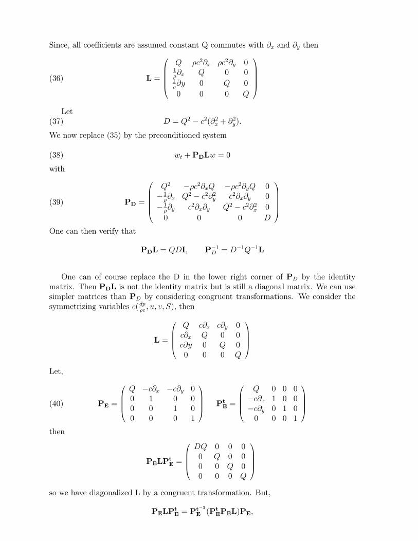
Since, all coe�cients are assumed constant Q commutes with @x and @y then

L =

0BBBB@Q �c2@x �c2@y 01�@x Q 0 0

1�@y 0 Q 0

0 0 0 Q

1CCCCA(36)

LetD = Q2 � c2(@2x + @2y):(37)

We now replace (35) by the preconditioned system

wt +PDLw = 0(38)

with

PD =

0BBBB@Q2 ��c2@xQ ��c2@yQ 0�1�@x Q2 � c2@2y c2@x@y 0

�1�@y c2@x@y Q2 � c2@2x 0

0 0 0 D

1CCCCA(39)

One can then verify that

PDL = QDI; P�1D = D�1Q�1L

One can of course replace the D in the lower right corner of PD by the identitymatrix. Then PDL is not the identity matrix but is still a diagonal matrix. We can usesimpler matrices than PD by considering congruent transformations. We consider thesymmetrizing variables c(dp

�c; u; v; S), then

L =

0BBB@Q c@x c@y 0c@x Q 0 0c@y 0 Q 00 0 0 Q

1CCCALet,

PE =

0BBB@Q �c@x �c@y 00 1 0 00 0 1 00 0 0 1

1CCCA PtE =

0BBB@Q 0 0 0�c@x 1 0 0�c@y 0 1 00 0 0 1

1CCCA(40)

then

PELPtE =

0BBB@DQ 0 0 00 Q 0 00 0 Q 00 0 0 Q

1CCCAso we have diagonalized L by a congruent transformation. But,

PELPtE = P

t�1

E (PtEPEL)PE;

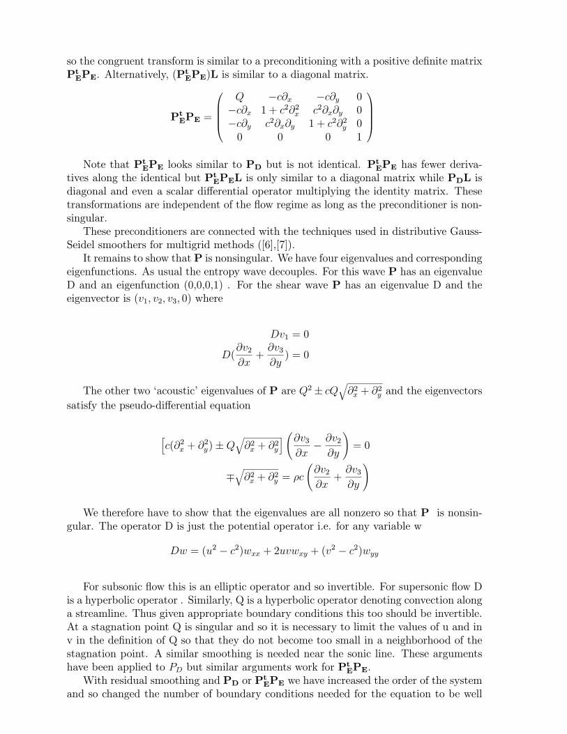
so the congruent transform is similar to a preconditioning with a positive de�nite matrixPtEPE. Alternatively, (P

tEPE)L is similar to a diagonal matrix.

PtEPE =

0BBB@Q �c@x �c@y 0�c@x 1 + c2@2x c2@x@y 0�c@y c2@x@y 1 + c2@2y 00 0 0 1

1CCCANote that PtEPE looks similar to PD but is not identical. P

tEPE has fewer deriva-

tives along the identical but PtEPEL is only similar to a diagonal matrix while PDL isdiagonal and even a scalar di�erential operator multiplying the identity matrix. Thesetransformations are independent of the ow regime as long as the preconditioner is non-singular.These preconditioners are connected with the techniques used in distributive Gauss-

Seidel smoothers for multigrid methods ([6],[7]).It remains to show that P is nonsingular. We have four eigenvalues and corresponding

eigenfunctions. As usual the entropy wave decouples. For this wave P has an eigenvalueD and an eigenfunction (0,0,0,1) . For the shear wave P has an eigenvalue D and theeigenvector is (v1; v2; v3; 0) where

Dv1 = 0

D(@v2@x

+@v3@y) = 0

The other two `acoustic' eigenvalues of P are Q2� cQq@2x + @

2y and the eigenvectors

satisfy the pseudo-di�erential equation

hc(@2x + @

2y)�Q

q@2x + @

2y

i @v3@x

� @v2@y

!= 0

�q@2x + @

2y = �c

@v2@x

+@v3@y

!

We therefore have to show that the eigenvalues are all nonzero so that P is nonsin-gular. The operator D is just the potential operator i.e. for any variable w

Dw = (u2 � c2)wxx + 2uvwxy + (v2 � c2)wyy

For subsonic ow this is an elliptic operator and so invertible. For supersonic ow Dis a hyperbolic operator . Similarly, Q is a hyperbolic operator denoting convection alonga streamline. Thus given appropriate boundary conditions this too should be invertible.At a stagnation point Q is singular and so it is necessary to limit the values of u and inv in the de�nition of Q so that they do not become too small in a neighborhood of thestagnation point. A similar smoothing is needed near the sonic line. These argumentshave been applied to PD but similar arguments work for P

tEPE.

With residual smoothing and PD or PtEPE we have increased the order of the system

and so changed the number of boundary conditions needed for the equation to be well

posed. To avoid this di�culty we do not solve the equation (38). Instead these precon-ditioners are used as a post processor for the usual Euler or Navier-Stokes equations.Thus, at each time step we calculate a residual based on one's favorite scheme. Thisgives a predicted value of the change in time, �wpredicted. We also update the boundaryconditions for the standard uid dynamic equations. We then operate on �w with Pwith the boundary condition that �wcorrected = 0 , i.e. we don't change the boundaryvalues calculated by the predictor. When we reach a steady state for the uids equationswe are solving P�wcorrected = 0 with zero boundary conditions. Since P is invertible�w = 0, i.e. we preserve the steady state. Thus, in essence we are imposing the uiddynamic boundary conditions between the P operator and the L operator.

6 Alternate Methods, Time Dependent Problems and Viscous Problems

The justi�cation for preconditioned schemes began with low Mach number ows. Forsuch ows other techniques exist beside preconditioning the equations. The method oftime inclining has similarities to preconditioning [15] .The basis of one such method is to use an implicit scheme. However, a two dimen-

sional implicit method is too expensive to be e�cient. Thus, one classically uses anADI approach. However, it is known that with ADI one cannot choose a very largetime step and converge quickly to the steady state. The splitting errors that occur inthe ADI method couples the waves together and one cannot choose an appropriate timestep for each wave. Instead one attempts to separate those terms in the equations thatcontribute to the fast acoustic waves from the slow components. One than can use asemi-implicit method which is implicit for the fast waves and explicit for the slow waves.Thus, the stability limit of the scheme is governed by the convective speed rather thanthe acoustic speed . The explicit part can be either a leapfrog method ([18], [19]), ora two step method [20]. This can also be extended to the Navier-Stokes equations [21].Alternatively, once these components are identi�ed, one can split the equations in severalpieces and solve each one separately as in the classical splitting methods [2] . In thiscase one can use an implicit method for the fast waves and an explicit method for theslow waves and in addition one can split o� the viscous terms. These methods work forboth time dependent and steady state problems.A di�erent alternative is to add terms to the equations which disappear in the steady

state. This has a connection with preconditioned methods when time derivatives areadded to the equations. However, in this approach other terms can be added besidetime derivatives. One example, is to assume that the total enthalpy is constant in thesteady state for the compressible inviscid equations. One can then add terms to theequations that depend on the deviation of the current enthalpy at each point from thisconstant steady state enthalpy [25]. For the incompressible equations one can add thedivergence of the velocity �eld or time derivatives of the divergence to the momentumequation [41], [43] . One can also consider a more general equation of state that reducesto the physical one at the steady state [44] . In [27] they analyze the general case of suchpseudo-unsteady systems.An extension of this technique is to modify the di�erential equation to remove the

acoustic waves or other `bad' features. One must then justify that the solutions ob-tained to these modi�ed equations are close to the original equations for some owregime. Typical examples are the various Low Mach number expansions for the uid dy-namic equations or the geostrophic equations as an approximation to the shallow water

equations in meteorology.For incompressible ow popular schemes are the SIMPLE [39] and MAC [22] algo-

rithms and their generalizations. These usually require the solution of a Poisson equationfor the pressure and then a pressure correction is used to update the momentum equa-tions. These methods can then be generalized to the compressible equations [24]. Merkle,Venkateswaran and Buelow [37] compare such methods to the preconditioned techniquesdiscussed in this paper. We again stress that the di�erence in these approaches is notwhether density or pressure are used as the dependent variable as one can transformbetween these variables. Thus, for example, one can modify the compressible continuityequation by replacing the time derivative of the density with a time derivative of thepressure. This is just another example of a matrix preconditioning as one can expressthe pressure derivative as a combination of a density derivative togther with momentumand energy derivatives. As described above, it is a programming decision whether oneshould use this modi�ed equation to update the pressure and then transfer to density orto calculate the the appropriate preconditioning matrix and update the density. For alinear system the two approaches are identical.For time dependent problems the �rst approach just discussed is useful. However,

the preconditioned methods and the second approach of this section destroy the timeaccuracy unless the coe�cients of the perturbation are chosen as a function of the meshsize and so only a�ect terms of the order of the accuracy of the scheme. A more popularapproach has been to use a two-time scheme. In this approach each new time levelis considered as the steady state of some problem. Alternatively, the physical timederivatives are considered a forcing terms. One now uses the preconditioned methods toachieve this `steady state' which in reality is the solution at the next time step. Hence,there is the physical time t and an arti�cial time � and � goes to in�nity as an innerloop within each time step. [12] , [47], [48]). Thus,

P�1@w

@�+@w

@t+@f

@x+@g

@y= 0:

The main di�culty with this approach is its e�ciency. It is reasonable to use sucha technique only if each `steady state' problem can be solved with little e�ort. Oneadvantage is that one usually has good initial guess for the solution based on the solutionat previous time steps. However, it typically takes 10 subiterations for each time step.Hence, this approach is ten times more expensive than a straight implicit method. Onecan also use an Newton iteration [38] at each time step. nevertheless, a semi-implicitapproach in ([18] - [21]) seems attractive.All the methods discussed thus far have been based on an inviscid analysis. For

the Navier-Stokes equations at high Reynolds number we do not expect any importantchanges outside the boundary layer. Inside the boundary layer viscous e�ects modify theeigenvalues of the di�erential operator. We thus wish to equalize the contribution of threequantities, the acoustic waves, the convective waves and the viscous terms. In particularthe viscous eigenvalues are very sti� and so the eigenvalues of the solution operatorare no longer well conditioned. All the preconditioners presented above depend on freeparameters (�; �; �; �) . Optimal values for these parameters were given for inviscid ow.A simple extension of the above methods to viscous ow would keep the same form forthe preconditioning matrices but allow these parameters to also depend on the Reynoldsor Prandtl number (see for example [10] ,[13] ). Thus, for example one �nds that for theoriginal pseudo-compressibility method that � should increase as the Reynolds number

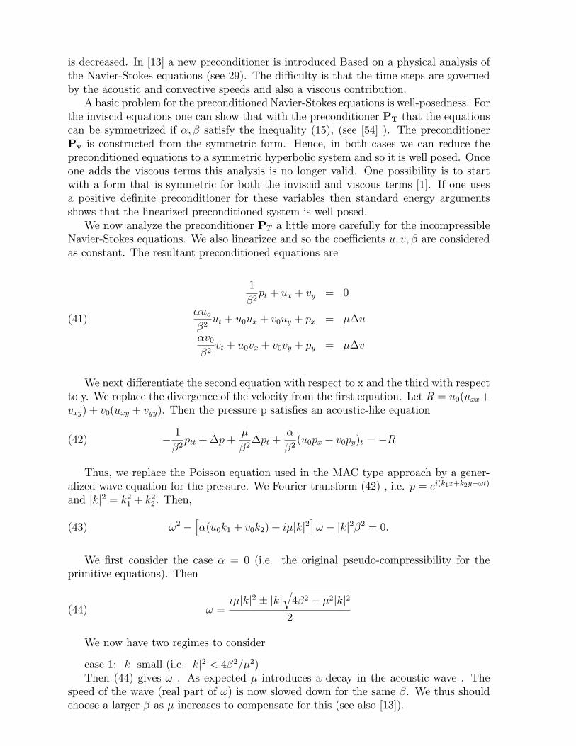
is decreased. In [13] a new preconditioner is introduced Based on a physical analysis ofthe Navier-Stokes equations (see 29). The di�culty is that the time steps are governedby the acoustic and convective speeds and also a viscous contribution.A basic problem for the preconditioned Navier-Stokes equations is well-posedness. For

the inviscid equations one can show that with the preconditioner PT that the equationscan be symmetrized if �; � satisfy the inequality (15), (see [54] ). The preconditionerPv is constructed from the symmetric form. Hence, in both cases we can reduce thepreconditioned equations to a symmetric hyperbolic system and so it is well posed. Onceone adds the viscous terms this analysis is no longer valid. One possibility is to startwith a form that is symmetric for both the inviscid and viscous terms [1]. If one usesa positive de�nite preconditioner for these variables then standard energy argumentsshows that the linearized preconditioned system is well-posed.We now analyze the preconditioner PT a little more carefully for the incompressible

Navier-Stokes equations. We also linearizee and so the coe�cients u; v; � are consideredas constant. The resultant preconditioned equations are

1

�2pt + ux + vy = 0

�uo�2ut + u0ux + v0uy + px = ��u(41)

�v0�2vt + u0vx + v0vy + py = ��v

We next di�erentiate the second equation with respect to x and the third with respectto y. We replace the divergence of the velocity from the �rst equation. Let R = u0(uxx+vxy) + v0(uxy + vyy). Then the pressure p satis�es an acoustic-like equation

� 1

�2ptt +�p+

�

�2�pt +

�

�2(u0px + v0py)t = �R(42)

Thus, we replace the Poisson equation used in the MAC type approach by a gener-alized wave equation for the pressure. We Fourier transform (42) , i.e. p = ei(k1x+k2y�!t)

and jkj2 = k21 + k22. Then,

!2 �h�(u0k1 + v0k2) + i�jkj2

i! � jkj2�2 = 0:(43)

We �rst consider the case � = 0 (i.e. the original pseudo-compressibility for theprimitive equations). Then

! =i�jkj2 � jkj

q4�2 � �2jkj2

2(44)

We now have two regimes to consider

case 1: jkj small (i.e. jkj2 < 4�2=�2)Then (44) gives ! . As expected � introduces a decay in the acoustic wave . The

speed of the wave (real part of !) is now slowed down for the same �. We thus shouldchoose a larger � as � increases to compensate for this (see also [13]).

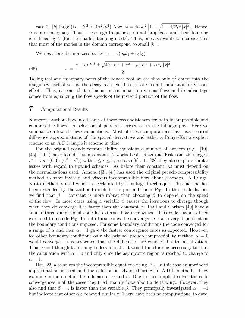
case 2: jkj large (i.e. jkj2 > 4�2=�2) Now, ! = i�jkj2h1�

q1� 4�2�2jkj2

i. Hence,

! is pure imaginary. Thus, these high frequencies do not propagate and their dampingis reduced by � (for the smaller damping mode). Thus, one also wants to increase � sothat most of the modes in the domain correspond to small jkj .

We next consider non-zero �. Let = �(u0k1 + v0k2)

! = + i�jkj2 �

q4�2jkj2 + 2 � �2jkj4 + 2i �jkj2

2:(45)

Taking real and imaginary parts of the square root we see that only 2 enters into theimaginary part of !, i.e. the decay rate. So the sign of � is not important for viscouse�ects. Thus, it seems that � has no major impact on viscous ows and its advantagecomes from equalizing the ow speeds of the inviscid portion of the ow.

7 Computational Results

Numerous authors have used some of these preconditioners for both incompressible andcompressible ows. A selection of papers is presented in the bibliography. Here wesummarize a few of these calculations. Most of these computations have used centraldi�erence approximations of the spatial derivatives and either a Runge-Kutta explicitscheme or an A.D.I. implicit scheme in time.For the original pseudo-compressibility equations a number of authors (e.g. [10],

[45], [11] ) have found that a constant � works best. Rizzi and Eriksson [45] suggest�2 = max(0:3; r(u2 + v2)) with 1 � r � 5, see also [9] . In [38] they also explore similarissues with regard to upwind schemes. As before their constant 0.3 must depend onthe normalizations used. Arnone ([3], [4]) has used the original pseudo-compressibilitymethod to solve inviscid and viscous incompressible ow about cascades. A Runge-Kutta method is used which is accelerated by a multigrid technique. This method hasbeen extended by the author to include the preconditioner PT. In these calculationswe �nd that � = constant is more robust than choosing � to depend on the speedof the ow. In most cases using a variable � causes the iterations to diverge thoughwhen they do converge it is faster than the constant �. Paul and Carlson [40] have asimilar three dimensional code for external ow over wings. This code has also beenextended to include PT. In both these codes the convergence is also very dependent onthe boundary conditions imposed. For some boundary conditions the code converged fora range of � and then � = 1 gave the fastest convergence rates as expected. However,for other boundary conditions only the original pseudo-compressibility method � = 0would converge. It is suspected that the di�culties are connected with initialization.Thus, � = 1 though faster may be less robust . It would therefore be neccessary to startthe calculation with � = 0 and only once the asymptotic region is reached to change to� = 1.Hsu [23] also solves the incompressible equations using PT. In this case an upwinded

approximation is used and the solution is advanced using an A.D.I. method. Theyexamine in more detail the in uence of � and �. Due to their implicit solver the codeconvergences in all the cases they tried, mainly ows about a delta wing.. However, theyalso �nd that � = 1 is faster than the variable �. They principally investigated � = �1but indicate that other �'s behaved similarly. There have been no computations, to date,

for the incompressible equations using the PV preconditioner due to the newness of thisapproach.For the compressible equations at low Mach numbers early calculations were done

by Briley, McDonald and Shamroth [8] and a later by D. Choi and Merkle [11], andalso Y.H. Choi and Merkle [34] . These methods have mainly used A.D.I. methodsthough some results with Runge-Kutta schemes have also been achieved. More recently([17],[55]) results have been achieved with the Pv preconditioner in conjunction with anupwind scheme. Godfrey (private communication) indicates that there is not a greatdi�erence between the two preconditioners. The use of the correct Riemann solver wasmore important than the details of the preconditioner.Much of the most recent work has gone into extending these results to the Navier-

Stokes equations [13] and chemistry ([17], [48], [58]). A number of authors have alsoinvestigated extensions to time dependent problems based on a two-time approach ([16],[48], [62]).Here we present only one set of results. This is for incompressible ow around a

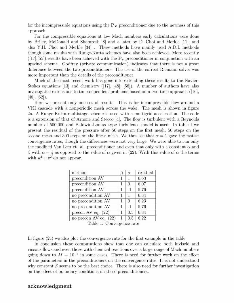
VKI cascade with a nonperiodic mesh across the wake. The mesh is shown in �gure2a. A Runge-Kutta multistage scheme is used with a multigrid acceleration. The codeis a extension of that of Arnone and Stecco [4]. The ow is turbulent with a Reynoldsnumber of 500,000 and Baldwin-Lomax type turbulence model is used. In table I wepresent the residual of the pressure after 50 steps on the �rst mesh, 50 steps on thesecond mesh and 300 steps on the �nest mesh. We thus see that � = 1 gave the fastestconvergence rates, though the di�erences were not very large. We were able to run onlythe modi�ed Van Leer et. al. preconditioner and even that only with a constant � and� with � = 1

2as opposed to the value of � given in (22). With this value of � the terms

with u2 + v2 do not appear.

method � � residualprecondition AV 1 1 6.63precondition AV 1 0 6.07precondition AV 1 -1 5.76no precondition AV 1 1 6.34no precondition AV 1 0 6.23no precondition AV 1 -1 5.76precon AV eq. (22) 1 0.5 6.34no precon AV eq. (22) 1 0.5 6.22

Table 1: Convergence rate

In �gure (2c) we also plot the convergence rate for the �rst example in the table.In conclusion these computations show that one can calculate both inviscid and

viscous ows and even those with chemical reactions over a large range of Mach numbersgoing down to M = 10�5 in some cases. There is need for further work on the e�ectof the parameters in the preconditioners on the convergence rates. It is not understoodwhy constant � seems to be the best choice. There is also need for further investigationon the e�ect of boundary conditions on these preconditioners.

acknowledgment

The author would like to thank Bram van Leer for many informative discussionsrelated to the topics discussed here.

References

[1] Abarbanel, S., and Gottlieb, D.,Optimal Time Splitting for Two and Three-Dimensional Navier-Stokes Equations with Mixed derivatives , Journal of Compu-tational Physics, Vol. 41, 1-33, 1981.

[2] Abarbanel, S., Dutt, P. and Gottlieb, D.,Splitting Methods for Low Mach NumberEuler and Navier-Stokes Equations , Computers Fluids, Vol. 17, 1-12, 1989.

[3] Arnone, A., Liou,M.-S., and Povinelli,L., Multigrid Calculation of Three Dimen-sional Viscous Cascade Flows , ICOMP report 91-18, 1991.

[4] Arnone, A., Stecco, S.S., Multigrid Calculation of Incompressible Flows for Turbo-machinery Applications , 24th Congress IAHR, Madrid, 1991.

[5] Au-Yeung, Y.H., A Theorem on a Mapping from a Sphere to the Circle and theSimultaneous Diagonalization of Two Hermitian Matrices Proc. Amer. Math. Soc.,Vol. 20, 545-548, 1969.

[6] Brandt, A., Multilevel Computations: Review and Recent Development , inMultigrid Methods: Theory, Applications and Supercomputing S. McCormick ed.,Marcel Dekker, 35-62, 1988.

[7] Brandt, A. , Guide to Multigrid Weizmaan Institute, 1984.

[8] Briley, W.R., McDonald, H.and Shamroth, S.J., A Low Mach Number Euler Formu-lation and Application to Time-Iterative LBI Schemes, AIAA J., Vol. 21, 1467-1469,1983.

[9] Cabuk, H., Sung, C.-H., and Modi, V., Explicit Runge-Kutta Method for Three-Dimensional Internal Incompressible Flows, AIAA J., Vol. 30, 2024-2031, 1992.

[10] Chang, J.L.C. and Kwak,D., On the Method of Pseudo Compressibility for Numer-ically Solving Incompressible Flows , AIAA paper 84-0252, 1984.

[11] Choi, D. and Merkle C.L., Application of Time-Iterative Schemes to IncompressibleFlow , AIAA J., Vol. 23, 1518-1524, 1985.

[12] Choi, Y.-H. and Merkle, C.L., Time-Derivative Preconditioning for Viscous Flows,AIAA paper 91-1652, 1991.

[13] Choi, Y.-H. and Merkle, C.L., The Application of Preconditioning to Viscous Flows,to appear Journal of Computational Physics,

[14] Chorin, A.J., A Numerical Method for Solving Incompressible Viscous Flow Prob-lems, Journal of Computational Physics, Vol.2, 12-26, 1967.

[15] Dannenho�er, III, J.F.and Giles, M.B., Accelerated Convergence of Euler SolutionsUsing Time Inclining , AIAA J., Vol. 28, 1457-1463, 1990.

[16] Feng, J. and Merkle, C.L., Evaluation of Preconditioning Methods for Time March-ing System , AIAA paper 90-0016, 1990.

[17] Godfrey, A.G., Walters. R.W. and Van Leer, B., Preconditioning for the NavierStokes Equations with Finite Rate Chemistry, to appear AIAA paper , 1993.

[18] Guerra, J., and Gusta�son, B., A Numerical Method for Incompressible and Com-pressible Flow Problems with Smooth Solutions , Journal of Computational Physics,Vol. 63, 377-397, 1986.

[19] Guerra, J., and Gusta�son, B., A Semi-implicit Method for Hyperbolic Problemswith Di�erent Time-scales , SIAM J. Numer. Anal. , Vol. 23, 734-749, 1986.

[20] Gusta�son, B., Unsymmetric Hyperbolic Systems and the Euler equations at LowMach Numbers , J. Scienti�c Computing, Vol. 2, 123-136, 1987.

[21] Gusta�son, B. and Stoor, H., Navier-Stokes Equations for Almost IncompressibleFlow , SIAM J. Numer. Anal., Vol. 28, 1523-1547, 1991.

[22] Harlow, F. H. and Welch, J.E., Numerical calculation of Time-Dependent ViscousIncompressible Flow with Free Surfaces , Physics of Fluids, Vol. 8, 2182-2185, 1965.

[23] Hsu, C.-H., Chen, Y.-M. and Liu, C.H., Preconditioned Upwind Methods to Solve3-D Incompressible Navier-Stokes Equations for Viscous Flows , AIAA J., Vol.30,550-552, 1991.

[24] Issa, R.I. , Solution of the Implicitly Discretized Fluid Flow equations by Operatorsplitting ,, Journal of Computational Physics, Vol. 62, 40-65, 1986.

[25] Jameson, A., Schmidt, W. and Turkel, E., Numerical Solutions of the Euler Equa-tions by a Finite Volume Method using Runge-Kutta Time-Stepping Schemes , AIAApaper 81-1259, 1981.

[26] Jameson, A. and Baker, T. J., Multigrid Solution of the Euler Equations for AircraftCon�gurations, AIAA Paper 84-0093, 1984.

[27] C. de Jouette, Viviand, H, Wornom,S. Le Gouez, J.M., Pseudo-CompressibilityMethods for Incompressible Flow Computation , Fourth International Symposiumon CFD, Davis, 270-274, 1991.

[28] Klainerman, S. and Majda, A., Compressible and Incompressible Fluids , Comm.Pure Appl. Math., Vol. 35, 629-651, 1982.

[29] Kobayashi, M.H. and Pereira, J.C.F., Predictions of Compressible Flows at all MachNumber Using Pressure Correction, Collocated Primitive Variables and Nonorthog-onal Meshes , AIAA paper 92-0426, 1992.

[30] Kreiss, H.O.and Lorenz, J., Initial-Boundary Value Problems and the Navier-Stokes Equations,Academic Press, Boston , 1989.

[31] Kreiss, H.O., Lorenz,J. and Naughton, M., Convergence of the Solutions of the Com-pressible to the Solutions of the Incompressible Navier-Stokes Equations , Advancesin Appl. Math., Vol. 12, 187-214, 1991.

[32] Lee, W.T , Local Preconditioning of the Euler Equations , Ph. D. Thesis, Universityof Michigan, 1991.

[33] Martinelli, L. and Jameson, A., Validation of a Multigrid Method for the ReynoldsAveraged Equations, AIAA Paper 88-0414, 1988.

[34] Merkle, C.L. and Choi, Y.H., Computation of Low-Speed Flow with Heat Addition ,AIAA J., 831-838. 1987.

[35] Merkle, C.L. and Choi, Y.H., Computation of Low-Speed Compressible Flows withTime Marching Procedures , International Journal for Numerical methods in Engi-neering, Vol. 25, 293-311, 1988.

[36] Merkle, C.L. and Athavale, M., A Time Accurate Unsteady Incompressible Algo-rithm Based on Arti�cial Compressibility , AIAA paper 87-1137, 1989.

[37] Merkle, C.L., Venkateswaran, S., Buelow, O.E., The Relationship Between Pressure-Based and Density-Based Algorithms , AIAA paper 92-0425, 1992.

[38] Pan, D. and Chakravarthy, S., Uni�ed Formulation for Incompressible Flows, AIAApaper 89-0122, 1989.

[39] Patanker, S.V. , Numerical Heat Transfer and Fluid Flow , Series in ComputationalMethods in Mechanics and Thermal Sciences, McGraw Hill, 1980.

[40] Paul, B.P. and Carlson, L.A., Analysis of Junction Flow�elds Using the Incompress-ible Navier-stokes Equations , AIAA paper 92-0519, 1992.

[41] Peyret, R. and Taylor, T., Computational Methods for Fluid Flow, Springer, NewYork, 1983.

[42] Peyret, R. and Viviand, H., Pseudo-Unsteady Methods for Inviscid or ViscousFlow Computations , Recent Advances in the Aerospace Sciences, Casci, C. edi-tor, Plenum, NY, 41-71, 1985.

[43] Ramshaw, J.D., Mesina, G.L., A Hybrid Penalty-Pseudocompressibility Method forTransient Incompressible Fluid Flow , Computers and Fluids, Vol. 20, 165-175,1991.

[44] Ramshaw, J.D., Mousseau, V.A. , Damped Arti�cial Compressibility Method forSteady-State Low-speed Flow Calculations , Computers and Fluids, Vol. 20, 177-189, 1991.

[45] Rizzi, A., Eriksson, L.E., Computation of Inviscid Incompressible Flow with Rota-tion J. Fluid Mechanics, Vol. 153, 275-312, 1985.

[46] Rogers, S.E., Kwak, D., Kaul, K.., On The Accuracy of the Pseudo CompressibilityMethod in Solving the Incompressible Navier-Stokes Equations , AIAA paper 85-1689, 1985.

[47] Rogers, S.E., Kwak, D., Kiris, C., Numerical Solution of the Incompressible Navier-Stokes Equations for Steady-State and Time Dependent Problems , AIAA paper89-0463, 1989.

[48] Shuen, J.-S., Chen, K.-H., and Choi, Y.H., A Coupled Implicit Method for ChemicalNon-Equilibrium Flows at All Speeds , Journal of Computational Physics

[49] Steger, J.L. and Kutler, P., Implicit Finite-Di�erence Procedures for the Computa-tion of vortex wakes , AIAA J., Vol. 15, 581-590, 1977.

[50] Swanson, R.C., Turkel, E., Pseudo-Time Algorithms for Navier-Stokes Equations ,Applied Numerical Math., Vol. 2, 321-334, 1986.

[51] Swanson, R.C., Turkel, E., On Central Di�erence and Upwind Schemes , Journalof Computational Physics, Vol. 101, 292-306, 1992.

[52] Taylor, L.K., Unsteady Three-Dimensional Incompressible Algorithm Based in Ar-ti�cial Compressibility , Ph.D. dissertation, Mississippi State, 1991.

[53] Turkel, E., Fast Solutions for Compressible Low Mach Flows and IncompressibleFlows , Ninth International Conf. Numerical Methods Fluid Dynamics, Springer-Verlag Lecture Notes in Physics, Vol. 218, pp. 571-575, 1984.

[54] Turkel, E., Preconditioned Methods for Solving the Incompressible and Low SpeedCompressible Equations , Journal of Computational Physics, Vol. 72, 277-298, 1987.

[55] Van Leer, B., Lee, W.T., Roe, P.L. , Characteristic Time-Stepping or Local Precon-ditioning of the Euler Equations , AIAA Paper 91-1552, 1991.

[56] Van Leer, B., Lee, W.T., Roe, P.L., Powell, K.G. , Design of Optimally SmoothingMultistage Schemes for the Euler Equations , Comm. Applied Numer. Meth., Vol.8, 1992.

[57] Venkateswaran,S. Weiss,J.M., Merkle,C.L. and Choi, Y.-H., Propulsion-RelatedFlow�elds Using the Preconditioned Navier-Stokes Equations , AIAA paper 92-3437,1992.

[58] Venkateswaran,S. Weiss,J.M., Merkle,C.L. and Choi, Y.-H., Preconditioning andTime-Step De�nition in Reacting Navier-Stokes Computations , submitted toAIAA J .

[59] Viviand, H., Pseudo-unsteady Systems for Steady Inviscid Flow Calculations , Nu-merical Methods for the Euler equations of Fluid Dynamics, F. Angrand et. al.editors, SIAM, 334-368. 1985.

[60] Volpe, G., On the Use and Accuracy of Compressible Flow Codes at Low MachNumbers , AIAA Paper 91-1662, 1991.

[61] Wigton, L.B. , Swanson R.C. On Variable Coe�cient Implicit Residual Smoothing,12th International Conf. Numerical Methods Fluid Dynamics, 1990.

[62] Withington, J.P., Shuen, J.S. and Yang, V., A Time Accurate Implicit Method forChemically Reacting Flows at All Mach Numbers, AIAA paper 91-0581, 1991.

[63] Zauderer, E., Partial Di�erential Equations Of Applied Mathematics, Wiley, NewYork , 1983.