REVIEW OF

QUEENSLAND’S OVERALL POSITION CALCULATIONS

George Cooney

September 2014

ii

EXECUTIVE SUMMARY

In the forty years since the abolition of external examinations in Queensland there have been several reforms of the senior years of schooling and of universities’ admission procedures. The use of school-based assessments rather than external examinations has given teachers greater power in the assessment of their students, both in the means by which students are assessed and in the way their achievements are reported. Marks and norm-referenced grades have been replaced by standard-referenced grades, and folios of work samples have replaced formal and school-based examinations. A further consequence has been that the responsibility for quality assurance is distributed to the system as a whole. The Queensland Studies Authority1, a statutory authority of the Queensland Government, is to be commended for the extensive combination of internal reviews, moderation meetings and external reviews that are undertaken, and for the extensive range of publications outlining the procedures. Universities’ admission procedures were the focus of reports in the late 1980s and early 1990s leading to the recommendation that the Tertiary Entrance Score be replaced with a Student Profile that would be used for tertiary admission by providing:

· a measure of overall achievement, termed the Overall Position (OP) · measures of achievement in specific fields of study, termed Field Positions (FP) · a measure of achievement on the Queensland Core Skills (QCS) test

Underpinning the recommendation was the belief that, although the Tertiary Entrance Score had many points of discrimination, not all represented significant differences in student achievement. This entrance score was subsequently replaced by the OP that was more consistent with the uncertainties in students’ scores and which provided the discrimination necessary of admission procedures for most generalist university courses. For high-demand courses the FPs provided the additional discrimination that was required for admission procedures in these courses. The calculation of OPs and FPs have much in common with the procedures in other jurisdictions; all have within and between school stages. In the ACT and Queensland, where there are no external examinations, the within-school stage puts students’ ranks from different subjects on a common within-school scale. The second stage rescales the ranks to put all schools on the same scale. In states with external examinations school-based assessments are first moderated to place them on a common scale across schools and an average of the examination marks and moderated assessment mark is further scaled to remove differences between subject candidatures. Underpinning the scaling process of all jurisdictions is the assumption that students’ marks or ranks in different subjects are correlated to the extent that a weighted or unweighted aggregate has some substantive meaning. Students with higher aggregates are deemed to have demonstrated more of what are termed higher cognitive skills so will therefore be better able to perform well at university. There are, however, several features in the Queensland procedures that are unique, including the centrality of grades rather than marks, the differential treatment of visa students and the redundancies in the process that underpin the excellent quality control over both inputs and outputs. Quality control is evident in all phases of the calculation of the OPs and FPs, from the initial data input to the final anomaly checks. Because of the importance of school-based grades, the annual and extensive state-wide review of school grades is an essential component of the Queensland procedure. SAIs are validated against levels of achievement and in the calculation of subject-group scaling parameters student’s scaling scores are weighted according to their relationship with their Within School 1 Renamed the Queensland Curriculum and Assessment Authority, June 2014

iii

Measures (WSMs). Finally schools’ rankings are validated against polyscores that are school rankings based on grades. The extent of the quality control routines comes with a cost. The calculation of students’ OPs is a very complex operation with a range of different statistical methods being used in the process. The actual scaling is based on a linear bivariate adjustment procedure, albeit using a weighted mean difference rather than the usual standard deviation to minimise the effect of outliers. The two non-parametric measures, the WSMs and polyscores, which are used for anomaly detection at individual, subject-group and school-group levels, are innovative but difficult to explain. Having said this I would not suggest reducing the redundancies in the calculations. They are necessary to ensure the quality of the process. In this audit of the calculation of Overall Positions and Field Positions I have evaluated the current procedures against the QSA’s published documents on their procedures using data provided by the QSA and other statistics. The various sources are listed in the Bibliography, and where tables or figures have been taken from a QSA publication they are referenced by footnotes. Other tables and figures are the result of analysis of data provided by the QSA. I am impressed by the range of measures designed to both identity anomalous observations at student, subject-group and school-group levels and to mitigate their influence on the calculations, and am also impressed by the care taken by QSA staff to ensure the accuracy of the calculations and hence of the OPs and FPs. The results of the analyses undertaken on the 2013 data are very similar to those from the 2012 data. The stability of the results and of the distributions of OPs and FPs are indicative of the quality of the calculations. My previous observations about fielding and the calculation of Item Field weights have, however, been confirmed. The principal components analysis of the QCS Test items show that while there are clear verbal and quantitative components in addition to a measure of general or overall achievement, the further division of each component into smaller components based on item type appears not to be warranted. The allocation of item weights to Field E is also problematic. In contrast to the simple structure apparent of the items weights for Fields A, B, C and D, all items load on Field E. The result is that the scaling score for Field E resembles a measure of overall achievement. There are at least two possible options that might address this situation: the first it to re-design the QCS test to include a greater proportion of extended response items and the second is to re-think the role of Field Positions in the admission process. The first option would necessarily change the nature of the QCS test. Currently the this test is different from other scaling tests in that it is a general achievement test based on the 49 elements of the Queensland senior secondary curriculum rather than a general ability test. This is a strength of the Queensland procedure, which should not be changed without serious consideration. In addition, given evidence from research into the structure of Year 12 examinations, any change in this direction may not necessarily change the two factor structure that is evident in the QCS test. The second option is to re-think the role of field positions. Available data indicates that the use of Field Positions in tertiary admission procedures in Queensland is limited. With the introduction of bonuses they may become redundant entirely. In relation to Field E, currently universities select students for courses that require performance skills in music, design, drama or other expressive arts on the basis of portfolios in addition to, or instead of, academic results. Consequently, if the purpose of Field E is to assist tertiary institutions to select students for these types of courses, it is unnecessary.

iv

In summary, field positions have been given an important role in the tertiary admission process since their inception but, given the changes that have occurred in university admission procedures and the complexity of the fielding process, perhaps it is time to re-think their role; whether to abolish them or reduce the number of fields to two. Having only verbal and quantitative fields would simplify the fielding process and give greater clarity to their role. These suggestions are for a time when changes in the structure of the last two years of secondary education in Queensland are mooted. Until that time I do not recommend any changes to the procedures, they are necessary and sufficient to ensure the accuracy of the calculations of the OPs and FPs. May I express my thanks to the QSA for inviting me to undertake this task, and to Brian Nott for his assistance with through reports, discussions and the provision of data, and for his patience. George Cooney 23rd September 2014

v

TABLE OF CONTENTS

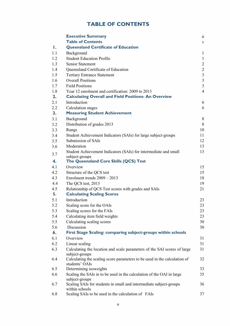
Executive Summary ii Table of Contents v 1. Queensland Certificate of Education 1.1 Background 1

1.2 Student Education Profile 1 1.3 Senior Statement 2 1.4 Queensland Certificate of Education 2 1.5 Tertiary Entrance Statement 3 1.6 Overall Positions 3 1.7 Field Positions 3 1.8 Year 12 enrolment and certification: 2009 to 2013 4

2. Calculating Overall and Field Positions- An Overview 2.1 Introduction 6 2.2 Calculation stages 6

3. Measuring Student Achievement 3.1 Background 8 3.2 Distribution of grades 2013 8 3.3 Rungs 10 3.4 Student Achievement Indicators (SAIs) for large subject-groups 11 3.5 Submission of SAIs 12 3.6 Moderation 13

3.7 Student Achievement Indicators (SAIs) for intermediate and small subject-groups

13

4. The Queensland Core Skills (QCS) Test 4.1 Overview 15

4.2 Structure of the QCS test 15 4.3 Enrolment trends 2009 – 2013 18 4.4 The QCS test, 2013 19 4.5 Relationship of QCS Test scores with grades and SAIs 21

5. Calculating Scaling Scores 5.1 Introduction 23 5.2 Scaling score for the OAIs 23 5.3 Scaling scores for the FAIs 23 5.4 Calculating item field weights 23 5.5 Calculating scaling scores 30 5.6 Discussion 30

6. First Stage Scaling: comparing subject-groups within schools 6.1 Overview 31 6.2 Linear scaling 31 6.3 Calculating the location and scale parameters of the SAI scores of large

subject-groups 31

6.4 Calculating the scaling score parameters to be used in the calculation of students’ OAIs

32

6.5 Determining isoweights 33 6.6 Scaling the SAIs in to be used in the calculation of the OAI in large

subject-groups 35

6.7 Scaling SAIs for students in small and intermediate subject-groups within schools

36

6.8 Scaling SAIs to be used in the calculation of FAIs 37

vi

6.9 Visa students 37 6.10 The result of scaling 37 6.11 Calculating the Overall Achievement Indicator 37 6.12 Calculating the Field Achievement Indicators 38 6.13 Relationship between OAIs and FAIs 40 6.14 Result of the first stage of scaling 40 7. Second Stage Scaling: Scaling Between Schools 7.1 Overview 41 7.2 Distribution of OAIs and FAIs in 2013 41 7.3 Anomaly detection at school-group level 42 7.4 Polyscores 43 7.5 Detecting anomalous schools 44 7.6 QSA intervention plots 45 8. Calculating Overall and Field Positions 8.1 Banding OAIs into OPs 48 8.2 Banding FAIs into FPs 48 8.3 Individual student anomaly detection 48 8.4 Discussion 50 9. Overall and Field Positions in 2013 9.1 Overall Positions in 2013 51 9.2 Gender differences in Overall Positions 52 9.3 Field Positions in 2013 53 9.4 Gender differences in Field Positions 55 9.5 Discussion 56 Bibliography 57

1

1. QUEENSLAND CERTIFICATE OF EDUCATION

1.1 Background Queensland has had a system of externally moderated school-based assessment in operation in various forms since the 1970 Radford Report2. One consequence of this change was that teachers were given greater power in the assessment of their students, using continuous school-based assessment programs to make judgements about the standards achieved by their students. A second consequence has been a move away from marks and norm-referenced grades and a move towards standards-based grades for both individual pieces of assessment and overall measures of achievement. Folios have replaced examinations for assessing students, and grades have replaced marks for reporting performance. A further consequence of the Radford and subsequent reports3 was that the responsibility for quality assurance has been distributed to the system as a whole. The Queensland Studies Authority (QSA), an independent statutory body of the Queensland Government, was given the responsibility for managing the system of externally moderated school-based assessment and senior secondary education. This organisation is to be commended for the extensive combination of internal reviews, moderation meetings and QSA-conducted external reviews that have been undertaken, and for the extensive range of publications outlining the procedures followed. Further reforms were implemented following the 1987 Pitman Report4 which discussed the perceived unfairness in the use of Tertiary Entrance scores to establish precise cut-offs for selection purposes, and proposed the use of coarser selection indices supplemented by special purpose indicators. These proposals were not implemented in their entirety but modified arrangements were put in place as a consequence of the 1990 Viviani Report.5 The major recommendation was the introduction of a Student Profile that would be used as a three-part method of university entrance by providing:

· a measure of each student’s overall achievement at school, expressed as a position on a rank order, called the Overall Position (OP)

· measures of their achievements in specific fields of study at school, also expressed as positions on five rank orders called Field Positions (FPs)

· students’ individual results in the new Core Skills (QCS) test The structure that finally emerged was a two stage admission process. Although QCS results are used in the calculation of OPs and FPs they are not directly used for admission purposes. 1.2 Student Education Profile Each year the QSA awards a Student Education Profile (SEP) to all students who complete Year 12 in Queensland. The SEP can comprise:

· a Senior Statement only, · a Senior Statement and Queensland Certificate of Education, or · a Senior Statement and Tertiary Entrance Statement, or · a Senior Statement, Queensland Certificate of Education, and Tertiary Entrance Statement.

2 Radford, W. (Chairman) 1970,Public Examinations for Queensland Public Schools, Queensland Department of Education, Brisbane. 3 Scott, E. (Chairman), 1878. A review of school-based assessment on Queensland secondary schools. Board of Secondary School Studies. Brisbane. 4 Pitman, J.A. 1987. Tertiary Entrance in Queensland: A Review 5 Viviani,I 1990. Tertiary Entrance in Queensland 1990.

2

1.3 Senior Statement

The Senior Statement shows all studies completed and the results achieved that contribute to the award of the Queensland Certificate of Education (QCS) or to the Tertiary Entrance Statement (TES). Students who are given a Senior Statement are regarded as having satisfied the completion requirements for Year 12 in Queensland. 1.4 Queensland Certificate of Education In their senior years students may undertake a wide range of learning experiences in a range of settings including schools, technical colleges, workplaces and the community; and students may also complete courses offered by tertiary institutions. The different studies are classified under the following four categories that are given different amounts of credit towards the QCE.

· Core · Preparatory · Enrichment · Advanced

To be eligible for the QCE students must:

· have gained at least 20 credits in the required pattern of courses · fulfilled specified literacy and numeracy requirements

A minimum of 12 credits must be completed in Core courses of study that can include:

· Authority or Authority-registered subjects6 - a minimum of a sound level of achievement standard is required

· Vocational education and training certificates – at least a complete AQF Certificate 1; incomplete certificates at higher levels attract additional credit

· University subjects studied while at school - a minimum pass standard is required · Recognised international courses of study - a minimum pass standard is required · Recognised awards and certificates · Workplace, community and self-directed learning at an approved standard

Results in these subjects are reported as one of the following five levels of achievement:

· Very High Achievement · High Achievement · Sound Achievement · Limited Achievement · Very Limited Achievement

The literacy and numeracy requirements can be met by satisfying a range of options including:

6 Authority subjects are courses based on syllabuses approved by the QSA, the results from which can be contribute to the calculation of OPs and FPs. Authority registered subjects are developed from study specifications and may include substantial vocational components but do not contribute to the calculation of OPs and FPs. Both types of subjects can be studies across four semesters, with each semester of study contributing four credits towards the QCE.

3

· Literacy: At least a sound level of achievement in one semester of English, English Extension, English Communication or English for ESL learners.

· Numeracy: At least a sound level of achievement in one semester of Mathematics A, Mathematics B, Mathematics C or Prevocational Mathematics.

1.5 Tertiary Entrance Statement

The Tertiary Entrance Statement (TES) includes eligible students’ OPs and FPs that are rankings used by tertiary institution to assist them in their admission procedures. The TES also provides information that is recognised by interstate and international universities and other tertiary institutions for admission purposes. 1.6 Overall Positions

Students’ OPs are state-wide ranks based on their overall achievement in Authority subjects, indicating how well they have performed in their senior subjects compared with the performance of other OP-eligible students in Queensland. To be eligible for an OP students must:

· complete at least 20 semester units of Authority subjects of which at least three of these subjects must be studied for four semesters

· complete the QCS test

There are 25 OP bands, from OP 1 (highest) to OP 25 (lowest) with each OP representing a group of students whose achievements are regarded as similar enough to place them in the same broad level of achievement. The band boundaries are determined each year so that each OP represents a fixed standard from year to year. Under the Education (Queensland Studies Authority) Regulation (2002) only citizens and permanent residents are eligible for OPs. Most international students who are on a student visa7 are not eligible for OPs or FPs, but if they satisfy the same eligibility requirements as domestic students in relation to the OP they can receive equivalent OPs and FPs.

1.7 Field Positions

Field Positions are state-wide ranks of OP-eligible students in specified fields of study that are provided to universities to aid admission to courses that require specific attributes. The five fields are:

7 For OP calculation purposes, visa students are those who live temporarily in Australia under a short-term visa or a similar authority issued by the Australian Government. If a student is a permanent resident of Australia (with a visa or not) they are not classed as a visa student for the purposes of tertiary entrance procedures. Visa students may include:

· scholarship, exchange or government-sponsored students from any overseas country · children of foreign diplomats · students admitted under the full-fee payment scheme · private students · children of parents who are in Australia as temporary residents (for instance, business people who work

in Australia for a limited period of time and who do not have Australian permanent residency or citizenship)

4

70%

75%

80%

85%

90%

2009 2010 2011 2012 2013

A extended written expression involving complex analysis and synthesis B short written expression involving reading, comprehension, and expression in English or

a foreign language C Basic numeracy involving simple calculations and graphical and tabular interpretation

D Solving complex problems involving mathematical symbols and abstractions E Substantial practical performance involving physical and creative arts or expressive skills

Eligibility for an FP depends on the combination of Authority subjects studied, and the number of weighted semesters completed. Students can be eligible for up to five FPs, depending on the number and nature of the subjects they have studied. A subject weight is allocated to each Authority subject for each of the five fields, which indicates the relative importance of that subject for that field. The weights lie between 1 (lowest) and 5 (highest) and, if the subject has no relationship with the field, the weight is given as N/A. The number of weighted semesters is calculated by multiplying the number of semesters by the subject weight. To be eligible for a particular field a student must has at least 60 weighted semesters in that field. There are ten bands for FPs, with 1 being the highest and 10 the lowest. 1.8 Year 12 enrolment and certification: 2009 to 20138

The size of the Year 12 cohort increased from 34,726 in 2009 to 43,211 in 2013. The percentage of students who received a QCE showed a similar proportionate increase.

Table 1: Number of students receiving the QCE by year, 2009 - 2013

Year 2009 2010 2011 2012 2013

N 34,726 37,193 39,582 41,398 43,211 Figure 1: Percentage of Year 12 students receiving QCE by year, 2009 - 2013

Year The following tables show the number of Year 12 students qualifying for the QCE, and who are OP-eligible for years 2009 to 2013. Data on OP-eligible students are given separately for domestic and visa students.

8 The data presented in this section have been taken from the 2013 Data summary: Year 12 enrolment and certification. Queensland Studies Authority 2014.

P

erce

ntag

e

5

0

20

40

60

80

100

Non-Visa Visa Total

2009 2010 2011 2012 2013

50%

60%

70%

80%

90%

2009 2010 2011 2012 2013

Domestic Visa

Table 2 and Figure 2 show that, although there has been an increase in the size of the Year 12 cohort and in the number of students receiving a QCE, there has not been a corresponding increase in the number of OP-eligible students. The numbers of OP-eligible students have changed little over the past five years, so that the percentage of OP-students has steadily declined in the domestic student cohort.

Figure 2: Percentage of OP-eligible students by visa status and year, 2009 – 2013

Table 2: Number of OP-eligible students by type of student and year, 2009 - 2013

2009 2010 2011 2012 2013

Domestic students Year 12 43,545 44,998 46,136 47,181 47,912

OP-eligible 25,305 25,703 25,947 26,233 25,883

OP- ineligible 18,240 19,295 20,189 20,948 22,029

Visa Students

Year 12 cohort 1,004 1,082 1,073 1,022 963

OP-eligible 812 862 868 790 728

OP-ineligible 192 220 205 232 235

All students

Year 12 cohort 44,549 46,080 47,209 48,203 48,875

OP-eligible 25,305 25,703 25,947 26,233 25,884 OP-ineligible 18,240 19,295 20,189 20,948 22,028

In contrast to the enrolment pattern of domestic students the number of Year 12 visa students has remained relatively constant over the past five years but the decline in the percentage of visa students eligible for an equivalent OP is similar to that of non-visa students.

Figure 3: Percentage of OP-eligible Year 12 students by visa status and year, 2009 - 2013

Pe

rcen

tage

Per

cent

age

6

7

2. CALCULATING OVERALL AND FIELD POSITIONS –

AN OVERVIEW

2.1 Introduction

OPs and FPs are state-wide rank orders. Students’ OPs are based on a measure of their overall achievement in senior secondary school studies that give equal weight to all subjects. FPs are state-wide rankings of OP-eligible students in specified fields of study which provide universities with finer discrimination between applicants for courses that require specific attributes. 2.2 Calculation stages There are five broad stages in the calculation of OPs and FPs:

A. Schools provide the QSA with a set of grades and Subject Achievement Indicators (SAIs) for each OP-eligible student. These are numbers lying between 200 and 400 that indicate students’ relative achievements in their subject-groups. Grades and SAIs are determined by teacher judgement, based on a range of within-school assessments. In large subject-groups9 in large school-groups10 at least one student must receive an SAI of 200 and one must receive a SAI of 400. The SAIs of the remaining students in the subject-group are distributed between these two numbers.

Students’ SAIs are scaled using scaling scores that are weighted aggregates of QCS test item scores. There are six scaling scores: one for the derivation of the Overall Achievement Indicator (OAI) which is based on students’ overall academic achievement, and five other scores for the derivation of the Field Achievement Indicators (FAIs) that are based on performance in the five fields.

All non-visa OP-eligible students will have a scaling score for the derivation of the OAI and one for each of the FAIs for which they are eligible. The first scaling score is the total score on the QCS test with all items weighted equally. In the calculation of the remaining scaling scores the items are weighted according to their importance in relation to the five fields. The weights are termed item field weights.

B. For each within-school subject-group two scaling parameters, the weighted mean and

mean difference11 of the scaling scores, are calculated. In the calculation of these scaling parameters students’ scaling scores are weighted according to the relationship of their QCS test scores with their Within-School Measures12 (WSMs). The weights are termed isoweights and make provision for students whose performance in the QCS test is aberrant.

9 Subject-groups are students in a school taking the same Authority subject and may comprise more than one class group. Subject-groups with more than 13 OP-eligible students who have studied the subject for more than one semester are termed large subject-groups, those with 10 to 13 OP-eligible students are termed intermediate subject-groups, and those with less than 10 OP-eligible students are termed small subject-groups. 10 Schools-groups are classified as large, intermediate or small according to the number of OP-eligible student enrolled: large (more than 19 students), intermediate (between 10 and 19 students), small (less than 10 students). 11 The mean difference is an alternative to the standard deviation, which is more stable than the standard deviation for small samples and when outliers are present. For large samples the mean difference is similar to the standard deviation. 12 WSMs indicate the positions of students in a school group relative to other students. It is based on their wins and losses in terms of their SAIs in the subjects they have completed. A win is when they have a higher SAI than other student is the subjects they have completed, a loss is when their SAI is lower. WSMs are calculated only for large school-groups and are scaled to the parameters of the school’s unweighted scaling score distribution.

8

For each subject-group there are up to six pairs of scaling parameters: the first pair for the derivation of the OP and the remaining pairs for the derivation of FPs that are related to that subject-group.

Linear transformations are used to scale the SAIs for each subject-group. For each SAI there will be up to six scaled SAIs: the first to be used for the OP calculation and the remaining used for the calculations of the FPs. The linear transformations are such that the means and mean differences of the SAIs of the OP-eligible students in a subject-group are the same as the means and mean differences of the appropriate scaling scores for these students in the subject-group.

C. Students’ scaled SAIs are averaged to determine their OAIs and the FAIs for which they

are eligible. Their OAIs are based on their best 20 semester units of credit on Authority subjects, including at least three subjects studied for four semesters. In the calculation of the FAIs each subject is weighted according to the importance of the subjects in relation to the five fields. These weights are termed subject weights.

D. Students’ OAIs are then rescaled using school-group scaling parameters, which are the

weighted means and mean differences of QCS test scores of school-groups. This final step is to make allowance for changes to the means or mean-differences of school-groups due to OAIs being based on the best 20 semester units rather than on all units completed. FIAs are not rescaled.

As a result of the second scaling stage rescaled OAIs are comparable across school-groups. As a quality control measure the QSA calculates alternate school-group rankings, termed polyscores, based on grades rather than OAIs. The two sets of school-group rankings are then compared to detect anomalous results at school-group level. Students in intermediate and small school-groups do not have their OAIs rescaled.

E. OAIs and FAIs are then banded into Overall Positions (OPs) and Field Positions (FPs):

25 bands for OPs and 10 bands for FPs. Students’ OPs are checked to detect anomalous results by comparing their OPs with OPs awarded to other students who have undertaken similar programs of study and who have similar grades and QCS test scores.

9

3. MEASURING STUDENT ACHIEVEMENT

3.1 Background

Underpinning the calculation of students’ OPs and FPs are grades and SAIs that are determined at the point at which students exit Year 12. Because of their importance and the primacy of teacher judgement, the QSA has in place an extensive system of processes to both assist teachers to make accurate judgements about student achievement and to check the quality of their decisions. Teachers record their judgments about the standards their students demonstrate on a range of assessment instruments, using numbers, letters or other symbols that show the match between the standards descriptors in the syllabus and the students’ responses on the various assessment tasks. When students exit Year 12 decisions are made about the overall standard they have achieved in each of the Authority subjects they have completed, which are based on students’ folios that contain responses to the range of assessment tasks they have completed during their course of study. In contrast to the practice in most other jurisdictions, holistic judgments are made in accordance with the syllabus requirements, rather than on marks from examinations and tests. All students are allocated grades that indicate the standards they have reached in their course: Very High Achievement, High Achievement, Sound Achievement, Limited Achievement and Very Limited Achievement. Teachers compare students’ work to published syllabus standards and the performance of other students is not relevant.

3.2 Distribution of grades 2013

Table 313 shows the distributions of grades in Authority subjects in 2013. Each subject has its own set of grade descriptors that specify the knowledge and skills that must be demonstrated to achieve each grade. Consequently, while the standards associated with the grades do not vary from one year to the next, there is no comparability of grades between different subjects. It follows that the percentages of students in the grades may be different for different subjects. Overall, 26.7% of grades awarded in 2013 were Very High Achievement, 34.0% were High Achievement, 29.6% Sound Achievement and 9.7% were Limited Achievement or Very Limited Achievement. Table 3: Distribution of grades in Authority subjects: Year 12 cohort 2013

N VHA HA SA LA VLA

% % % % % Aboriginal & Torres Strait Islander Studies 126 4.0 21.4 45.2 19.8 9.5

Accounting 3,907 23.6 31.7 28.0 12.6 4.2

Aerospace Studies 245 15.9 33.1 35.5 13.9 1.6

Agricultural Science 633 10.4 30.3 39.0 15.8 4.4

Ancient History 4,480 16.2 33.4 36.2 12.3 1.9

Biology 13,943 13.6 36.7 38.0 10.5 1.2 Business Communications & Technologies 5,782 14.6 37.0 36.6 10.5 1.4

Business Organisations & Management 2,723 18.4 37.9 32.4 10.4 0.9

Chemistry 9,710 15.9 34.1 37.0 11.2 1.7

Chinese 635 63.8 21.9 9.9 4.1 0.3

13 2013 subject enrolments and levels of achievement. page 9 Queensland Studies Authority 2014.

10

Table 3: Distribution of grades in Authority subjects: Year 12 cohort 2013 (contd)

N VHA HA SA LA VLA

% % % % %

Chinese Extension 66 66.7 30.3 3.0 0.0 0.0

Dance 2,000 21.3 33.9 33.5 10.0 1.5

Drama 5,967 21.5 39.6 29.7 7.9 1.3

Earth Science 407 9.1 41.3 40.1 8.6 1.0

Economics 2,488 21.7 39.2 31.8 6.4 0.9

Engineering Technology 736 18.1 31.4 35.3 14.1 1.1

English 34,809 13.2 37.7 40.5 8.1 0.5

English Extension 643 40.8 40.6 15.6 3.0 0.2

English for ESL Learners 571 8.1 35.6 47.5 7.5 1.4

Film, Television & New Media 3,755 17.6 34.4 34.9 11.2 1.9

French 912 39.1 38.8 18.0 3.7 0.3

French Extension 45 46.7 48.9 4.4 0.0 0.0

German 480 40.8 39.0 17.1 2.3 0.8

German Extension 33 57.6 33.3 9.1 0.0 0.0

Graphics 4,549 17.8 31.3 36.0 12.2 2.8

Health Education 2,146 13.4 31.9 38.0 14.4 2.4

Home Economics 2,993 11.9 30.1 41.3 13.8 2.9

Hospitality Studies 786 13.7 36.0 36.8 12.1 1.4

Indonesian 59 35.6 35.6 25.4 3.4 0.0

Indonesian Extension 4 25.0 50.0 25.0 0.0 0.0 Information Processing &Technology 2,786 14.3 32.5 36.4 13.6 3.3

Italian 298 43.0 34.2 19.8 2.7 0.3

Japanese 1,649 40.6 31.1 19.0 8.2 1.1

Korean 15 80.0 6.7 13.3 0.0 0.0

Latin 23 73.9 26.1 0.0 0.0 0.0

Legal Studies 6,120 15.3 32.5 37.3 12.9 2.1

Marine Studies 1,939 11.8 36.1 42.1 9.4 0.7

Mathematics A 26,514 10.9 32.6 42.5 12.4 1.7

Mathematics B 17,388 19.7 28.8 37.6 12.5 1.4

Mathematics C 4,564 30.4 34.2 27.2 7.5 0.8

Modern Greek 14 50.0 21.4 28.6 0.0 0.0

Modern History 5,494 19.1 33.9 33.8 11.3 1.9

Music 3,417 36.4 33.0 24.6 5.1 1.0

Music Extension 994 55.3 31.4 12.6 0.7 0.0

Philosophy & Reason 390 33.1 41.8 20.0 4.9 0.3

Physical Education 10,888 11.1 43.6 38.2 6.8 0.3

Physics 7,166 17.1 33.1 37.0 11.4 1.4

Science21 2,062 7.8 26.8 43.3 17.3 4.8

Spanish 125 32.0 33.6 30.4 4.0 0.0

Study of Religion 5,049 17.1 37.2 36.6 8.3 0.8

Study of Society 794 10.6 35.5 37.3 13.9 2.8

Technology Studies 1,741 15.5 33.1 36.2 12.4 2.8

Vietnamese 15 46.7 46.7 6.7 0.0 0.0

Visual Arts 6,895 14.3 31.7 38.1 13.5 2.5

11

Although the levels of achievement are standard-based grades, they provide information about students’ ranks and the relative differences between them. Since the same standards apply across all schools, levels of achievement can be compared across schools and therefore convey the same information as do the marks from state-wide examinations used in other jurisdictions. There were few differences in the distributions of subject grades between 2013 and 2014.

3.3 Rungs

Because the grades are broad levels of achievement, it is to expected that not all students on the same grade will be at the same standard so students are allocated to rung placements that indicate their positions within the grades. There are ten rungs within each grade so rung 8 indicates that the standard demonstrated is closer to that of grade 9 rather than that of grade 7. If students were uniformly distributed across the rungs within grades, there would be approximately 2% of the students in a subject-group on each rung. In a large subject-groups it would therefore be expected that there may be differences in achievement between students on the same rung. The following tables (Tables 4 and 5) show the distribution of grades for OP-eligible students who studied English in 2013 and the distribution of students across the rungs within the grades.

Table 4: Distribution of grades for OP-eligible in English, 2013

Table 5: Distribution of rungs within grades for OP-eligible students in English, 2013

RUNG Grade 1 2 3 4 5 6 7 8 9 10

Very High Achievement 25% 20% 16% 13% 10% 6% 4% 3% 1% 1%

High Achievement 13% 11% 11% 11% 11% 9% 9% 9% 8% 8%

Sound Achievement 7% 6% 8% 9% 11% 10% 11% 12% 11% 14%

Low Achievement 1% 1% 1% 2% 6% 7% 11% 18% 18% 35%

Very Low Achievement 10% 20% 30% 20% 10% 10%

Total 13% 11% 11% 11% 11% 9% 9% 9% 8% 9%

The difference between the grade distributions for English given in Table 3 and those given in Tables 4 and 5 is because Table 3 includes non-eligible students who are likely to be academically less able than their OP-eligible counterparts. It is therefore not surprising that there will be a higher percentage of OP-eligible students with higher grades. Table 5 shows that students in the Sound Achievement grade are distributed rather uniformly across the rungs. In the highest grade there are fewer students in the high rungs (6% - 10%) and more students closer to the High Achievement/Very High Achievement boundary. The converse is true for students awarded a Low Achievement grade.

N %

Very High Achievement 4,488 17.4

High Achievement 11,775 45.7

Sound Achievement 8,992 34.9

Low Achievement 491 1.9

Very Low Achievement 10 0.0

12

3.4 Student Achievement Indicators (SAIs) for large subject-groups

In large subject-groups it is likely that there will be students in the same rung with who have reached different standards, and a measure providing finer discrimination is required. SAIs are not marks, but are numbers awarded to OP-eligible students that indicate students’ positions in the subject-group in relation to other students. In large subject-groups the best student is always awarded an SAI of 400, and the worst student is awarded an SAI of 200. The remaining SAIs are then distributed between 200 and 400 to indicate students’ ranks and how close they are to each other. Teachers are expected to use professional judgement based on students’ portfolios rather than marks, and the use of pair-wide comparisons is encouraged14. There are some obvious implicit relationships between grades and SAIs. One would expect that, allowing for students on the same rung of a grade to have different SAIs, there would be a monotonic relationship between the two sets of ranks. One would also expect that students with similar grades would be closer to each other on the SAI scale than students with different grades. This is illustrated in the following table. Table 6 shows the distribution of SAIs for a large English subject-group in 2013 and the relationship between SAI, grade and rung. The two lowest students are assessed as demonstrating the same standard and given the same grade, rung and SAI. Eight students are awarded a Sound Achievement grade but are spread across the ten rungs. Students 3 and 4 are in the same rung but student 4 is ranked above student 3 so their SAIs are different. Students 5 and 6 are assessed to have reached the same standard, students 7 and 8 differ slightly. Student 9 is seen as close to students 7 and 8 but different enough to be placed in the next rung. Student 10 is perceived as very different from student 9 but whose achievement was not sufficient to be placed in the next grade. The top three students are spread across three rungs in the top grade.

Table 6: Distribution of English SAIs for a large subject group (n = 17)

Student Grade Rung SAI Student Grade Rung SAI

1 LA 5 200 9 SA 6 256 2 LA 5 200 10 SA 10 282 3 SA 1 230 11 HA 4 308 4 SA 1 231 12 HA 6 320 5 SA 4 244 13 HA 7 327 6 SA 4 244 14 HA 8 334 7 SA 5 251 15 VHA 3 374 8 SA 5 252 16 VHA 4 381

17 VHA 6 400

The relationship is also illustrated in Figure 6. As SAIs are within-school ranks they cannot be compared across schools. The top student in a large subject-group within a school will receive a SAI of 400 irrespective of the grade awarded. Table 7, which shows the minimum and maximum SAIs for OP-eligible students in English by grade awarded in 2013, illustrates the one to many mapping. Students awarded SAIs of 400 are

14 Subject Achievement Indicators (SAIs) Fact Sheet 1: the basics

13

0

50

100

150

200

250

300

350

400

LA LA SA SA SA SA SA SA SA SA HA HA HA HA VHA

VHA

VHA

spread across the top two grades, and students awarded SAIs of 200 are spread across the bottom three grades. In contrast, grades have a common meaning across schools. In these respects SAIs have a similar role to unmoderated school-based assessments in other jurisdictions, and the Queensland grades have a role similar to marks from external examinations. Figure 6: Relationship between SAI, rung and grade for large subject group (n=17)

Table 7: Distribution of SAIs for OP-eligible English students by grade awarded, 2013

Grade Mean Minimum Maximum VHA 361.3 303 400 HA 298.6 225 400 SA 242.2 200 319 LA 212.1 200 253

VLA 200.2 200 202

3.5 Submission of SAIs

Schools submit the grades and SAIs to the QSA on Form R6 as shown in Table 8. A computer program, BonSAI, has been developed to assist teachers to assign SAIs to their students. The completed forms are submitted to the QSA whose staff use BonSAI15 to check the alignment of SAIs to grades according to the following guidelines:

· If students have the same or similar level of achievement based on their allocated grade and rung, their SAIs should be close together.

· The difference between the average points (SAIs) per rung should increase from the lower levels of achievement to the higher levels of achievement. It is assumed that students’ work in the lower levels of achievement is likely to be more similar than students’ work in the higher levels of achievement.

15 Subject Achievement Indicators (SAIs) Fact Sheet 2: BonSAI. Queensland Studies Authority 2014.

Grade

SA

I

Grades

14

· The difference in the average points (SAIs) per rung in different parts of the distribution the difference will never be double. For example, if the average points per rung in LA is 2.1, points per rung should never be 4.2 or greater anywhere else in the distribution.

Table 8: Hypothetical example of Form R616

Family name Given name OP-

eligible Grade Rung SAI

OP VH 6 400 OP VH 3 373 OP HA 10 344 OP HA 5 317 OP SA 10 289 OP SA 10 287 OP SA 10 285 OP SA 8 278

OP LA 5 200

If anomalies are detected in a school’s distribution of SAIs, schools are contacted for clarification17. In 2013 273 schools were contacted about 1,280 distributions. A total of 400 were initially about clerical inconsistencies, not necessarily about problems with distributions.

3.6 Moderation

The anomaly check on SAIs is one phase of the QSA’s moderation procedures that are described below, which are designed to:

· support the integrity of school-based assessment in Authority subjects · strengthen the quality of teacher judgments of student achievement · ensure a high degree of comparability in the allocation of grades · maintain the credibility and acceptability of the SEP

The key phases of moderation are monitoring, verification, confirmation and random sampling. Monitoring of Year 11 folios occurs at the end of the first half of the two year program whereby review panels evaluate schools’ delivery and assessment of their courses and school judgments on a sample of Year 11 folios. Verification occurs towards the end of Year 12 when schools submit samples of student folios and details of interim levels of achievement in all Authority subjects they offer to the relevant review panel

16 Form R6. Queensland Studies Authority 2014. 17 Subject Achievement Indicators (SAIs) Fact Sheet 3: How QSA checks SAIs. Queensland Studies Authority 2014.

15

Confirmation occurs at the end of Year 12 when schools submit the levels of achievement and SAIs to the QSA that are described in the previous section. This phase concludes when the QSA reaches agreement with schools on the proposed results for recording on students’ Senior Statements. Random Sampling occurs after the SEPs have been distributed to evaluate how consistently teachers apply state-wide standards in determining students’ levels of achievement in Authority subjects. This extensive state-wide review of school grades based on samples of student work has been conducted each year since 1994. Random sampling refers to schools and students; subjects are selected on the basis of their size, stage of implementation or implementation issues. The 201318 random sampling review of assessment in Authority subjects included the review of 3,136 student folios from 456 submissions involving a total of 238 schools across 21 subjects. The reported findings showed that overall there was substantial agreement between panels and schools, with 91% of the judgements of folios being placed on the same level of achievement by both the random sampling panel and the school; 94% differed by less than four rungs. What was termed serious disagreement (eight or more rung differences) was recorded for 1% of folios. The subjects with the highest number of folios with rung differences of three or more were Information Technology Systems (14%), Graphics (23%), Physics (7%) and Drama (7%). Base on the level of disagreement recorded by random sampling panels, 36 submissions were requested for further review. The findings for the 2013 random sampling review were consistent with the findings from the 2012 review.

3.7 Student Achievement Indicators (SAIs) for intermediate and small

subject-groups For small and intermediate subject-groups with less than 14 OP-eligible students, rungs are used for SAIs. With small numbers rungs provide the appropriate level of discrimination between students and are more stable than separate SAIs.

18 Random sampling project. 2013 Report on random sampling of assessment in Authority subjects. Queensland Studies Authority 2014.

16

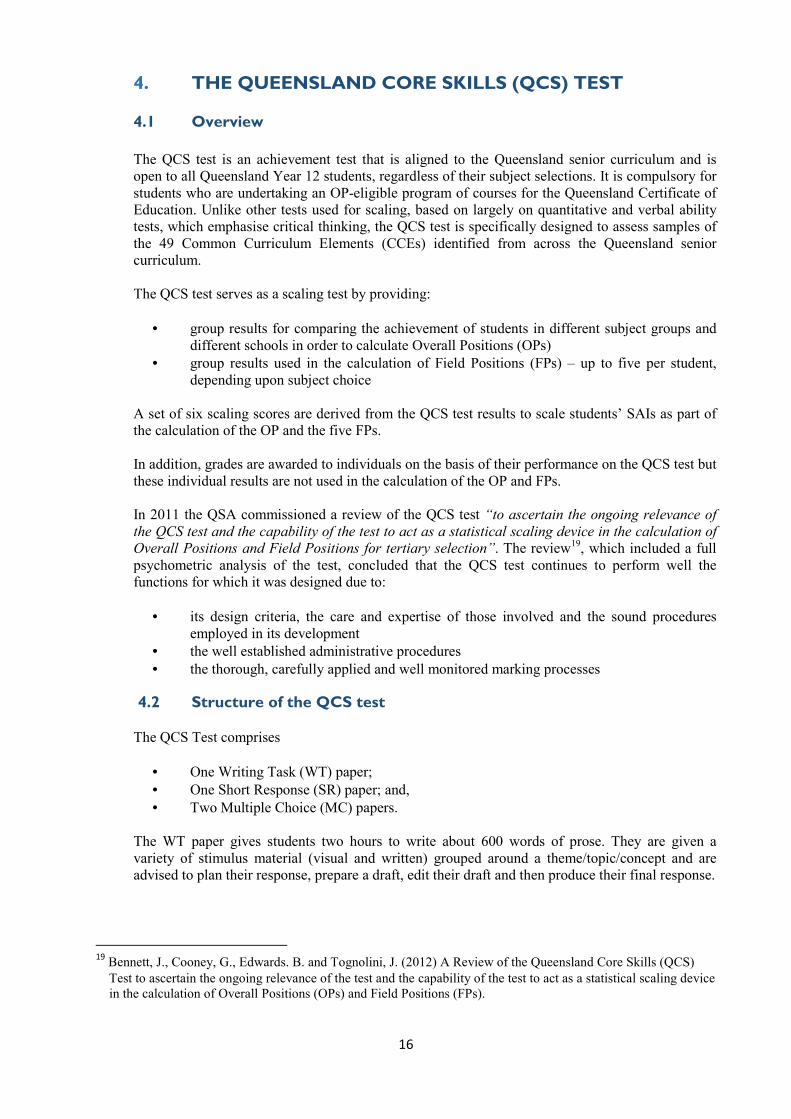
4. THE QUEENSLAND CORE SKILLS (QCS) TEST 4.1 Overview The QCS test is an achievement test that is aligned to the Queensland senior curriculum and is open to all Queensland Year 12 students, regardless of their subject selections. It is compulsory for students who are undertaking an OP-eligible program of courses for the Queensland Certificate of Education. Unlike other tests used for scaling, based on largely on quantitative and verbal ability tests, which emphasise critical thinking, the QCS test is specifically designed to assess samples of the 49 Common Curriculum Elements (CCEs) identified from across the Queensland senior curriculum. The QCS test serves as a scaling test by providing:

· group results for comparing the achievement of students in different subject groups and different schools in order to calculate Overall Positions (OPs)

· group results used in the calculation of Field Positions (FPs) – up to five per student, depending upon subject choice

A set of six scaling scores are derived from the QCS test results to scale students’ SAIs as part of the calculation of the OP and the five FPs. In addition, grades are awarded to individuals on the basis of their performance on the QCS test but these individual results are not used in the calculation of the OP and FPs. In 2011 the QSA commissioned a review of the QCS test “to ascertain the ongoing relevance of the QCS test and the capability of the test to act as a statistical scaling device in the calculation of Overall Positions and Field Positions for tertiary selection”. The review19, which included a full psychometric analysis of the test, concluded that the QCS test continues to perform well the functions for which it was designed due to:

· its design criteria, the care and expertise of those involved and the sound procedures employed in its development

· the well established administrative procedures · the thorough, carefully applied and well monitored marking processes

4.2 Structure of the QCS test The QCS Test comprises

· One Writing Task (WT) paper; · One Short Response (SR) paper; and, · Two Multiple Choice (MC) papers.

The WT paper gives students two hours to write about 600 words of prose. They are given a variety of stimulus material (visual and written) grouped around a theme/topic/concept and are advised to plan their response, prepare a draft, edit their draft and then produce their final response.

19 Bennett, J., Cooney, G., Edwards. B. and Tognolini, J. (2012) A Review of the Queensland Core Skills (QCS) Test to ascertain the ongoing relevance of the test and the capability of the test to act as a statistical scaling device in the calculation of Overall Positions (OPs) and Field Positions (FPs).

17

The SR paper gives students two hours to respond to a number of items that relate to stimulus material that cover many CCEs. The responses to items can vary, including mathematical or a visual expression, a sentence, a paragraph, or a longer prose piece. The two MC papers contain 50 items each and students are given 90 minutes to complete each paper. The items have a stem and four response options. The items are presented individually or in units based on common stimulus material. The material is drawn from a range of disciplines including language, literature, philosophy, history, the physical and life sciences, the social sciences, art and mathematics. The MC papers test the 49 CCEs embedded in the senior curriculum rather than the content that defines the subject.

Test items are grouped into five baskets20 according to how they test a student’s ability to:

α comprehend and collect β structure and sequence θ analyse, assess and conclude π create and present φ apply techniques and procedures.

The following table shows the CCEs categorised by baskets. Table 9: Common Curriculum Elements by basket21

α Comprehend and collect

1 Recognising letters, words and other symbols

2 Finding material in an indexed collection

3 Recalling/remembering

4 Interpreting the meaning of words or other symbols

5 Interpreting the meaning of pictures/illustrations

6 Interpreting the meaning of tables or diagrams or maps or graphs

7 Translating from one form to another

12 Compiling lists/statistics

13 Recording/noting data

28 Empathising

51 Identifying shapes in two and three dimensions

52 Searching and locating items/information

53 Observing systematically

55 Gesturing

57 Manipulating/operating/using equipment

β Structure and sequence

21 Structuring/organising extended written text

22 Structuring/organising a mathematical argument

29 Comparing, contrasting

30 Classifying

31 Interrelating ideas/themes/issues

36 Applying strategies to trial and test ideas and procedures

20 Queensland Core Skills Test 2013 Yearbook, page 6. Queensland Studies Authority 2014. 21 Queensland Core Skills Test 2013 Yearbook, page 9. Queensland Studies Authority 2014.

18

38 Generalising from information

49 Perceiving patterns

50 Visualising

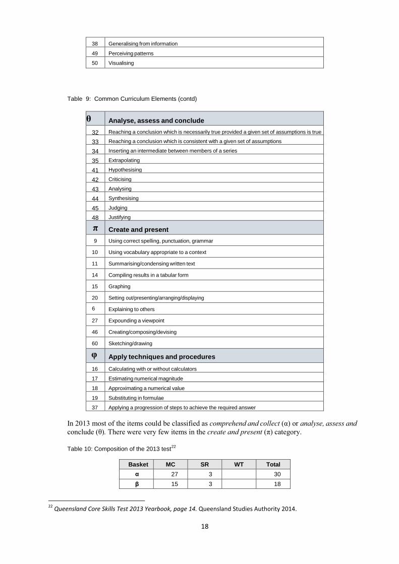
Table 9: Common Curriculum Elements (contd)

θ Analyse, assess and conclude

32 Reaching a conclusion which is necessarily true provided a given set of assumptions is true

33 Reaching a conclusion which is consistent with a given set of assumptions

34 Inserting an intermediate between members of a series

35 Extrapolating

41 Hypothesising

42 Criticising

43 Analysing

44 Synthesising

45 Judging

48 Justifying

π Create and present 9 Using correct spelling, punctuation, grammar

10 Using vocabulary appropriate to a context

11 Summarising/condensing written text

14 Compiling results in a tabular form

15 Graphing

20 Setting out/presenting/arranging/displaying

6 Explaining to others

27 Expounding a viewpoint

46 Creating/composing/devising

60 Sketching/drawing

φ Apply techniques and procedures

16 Calculating with or without calculators

17 Estimating numerical magnitude

18 Approximating a numerical value

19 Substituting in formulae

37 Applying a progression of steps to achieve the required answer

In 2013 most of the items could be classified as comprehend and collect (α) or analyse, assess and conclude (θ). There were very few items in the create and present (π) category. Table 10: Composition of the 2013 test22

Basket MC SR WT Total α 27 3 30 β 15 3 18

22 Queensland Core Skills Test 2013 Yearbook, page 14. Queensland Studies Authority 2014.

19

θ 39 4 43 π 4 2 1 7 φ 15 5 20

Total 100 17 1 118 Correlations between the subtests of the QCS test are given below (Table 11). As might be expected the correlation of the Writing Task with the other subtests and with the QCS test as a whole is the lowest overall. The MC and SR items are strongly correlated. Table 11: Correlations between subtests of QCS test, 2013

MC SR WT Total MC 1.000 0.819 0.499 0.934 SR 0.819 1.000 0.499 0.919 WT 0.499 0.499 1.000 0.708 Total 0.934 0.919 0.708 1.000

Table 12: Correlations between the baskets of items, 201323

α β θ π φ QCS α 1.000 0.660 0.737 0.487 0.641 0.826 β 0.660 1.00 0.718 0.476 0.636 0.828 θ 0.737 0.718 1.000 0.537 0.678 0.904 π 0.487 0.476 0.537 1.000 0.424 0.612 φ 0.641 0.636 0.678 0.424 1.000 0.795

QCS 0.826 0.828 0.904 0.612 0.795 1.000 The correlations between the baskets are varied, with baskets α, β and θ being strongly correlated. Basket π has the lowest correlations with the five baskets. As each subset of items is included in the QCS test scores, all baskets except for π are strongly correlated with the total score.

4.3 Enrolment trends 2009 – 2013 Students who are OP–eligible are obliged to sit for the QCS test. Students who are ineligible for the OP or who are eligible for an equivalent OP do not have to sit for the QCS test but may elect to do so. Tables 13 and 14 and the accompanying graphs show the percentage of different types of students sitting for the QCS test during the period 2009 to 201324.

Table 13: QCS candidature by OP eligibility, 2009 – 2013, non-visa students

Year Received SEP OP-eligible Sat QCS

Sat QCS test-

exempt1

Ineligible who sat Did not sit2

2013 47,910 25,883 27,794 437 2,348 1,448

2012 47,181 26,233 28,365 474 2,606 1,372

2011 46,136 25,947 28,326 503 2,882 1,489

2010 44,998 25,703 28,420 453 3,170 1,195

2009 43,545 25,305 28,301 397 3,393 1,100 1 OP eligible students who were exempt but nevertheless sat the QCS test 2 Students who were otherwise OP-eligible but did not sit for QCS test

23 Queensland Core Skills tests 2013 Yearbook, page 26. Queensland Studies Authority 2014. 24 QCS Attendance patterns 2013, page 2. Queensland Studies Authority 2014.

20

0.0%

10.0%

20.0%

30.0%

40.0%

50.0%

60.0%

70.0%

2009 2010 2011 2012 2013

% OP eligible % QCS

0.0%

20.0%

40.0%

60.0%

80.0%

100.0%

2009 2010 2011 2012 2013

% OP eligible % QCS

In contrast to visa students, the number of non-visa students who received a SEP increased in number from 2009 to 2013 but the number of QCS test candidates remained steady and the number of OP-eligible students declined. This trend has been evident since 1992.

The following figures show clearly the decline in the percentage of OP-eligible students and the percentage of QCS test candidates over the period 2009 to 2013. Table 14: QCS candidature by OP eligibility, 2009 – 2013, visa students

Year Received SEP OP-eligible Sat QCS

Sat QCS test-

exempt1

Ineligible who sat Did not sit1

2013 963 728 736 27 35 59

2012 1,022 790 819 6 35 37

2011 1,073 868 892 9 33 39

2010 1,082 862 892 17 47 45

2009 1,004 812 845 8 41 48 1 OP eligible students who were exempt but nevertheless sat the QCS test 2 Students who were otherwise OP-eligible but did not sit for QCS test

Figure 7: Percentage of QCS test candidates and percentage of OP-eligible students, 2009 – 2013, non- visa students

Figure 8: Percentage of QCS test candidates and percentage of OP-eligible students, 2009 – 2013, visa students

P

erce

ntag

e

P

erce

ntag

e

21

0

10

20

30

40

A B C D E

Male Female All

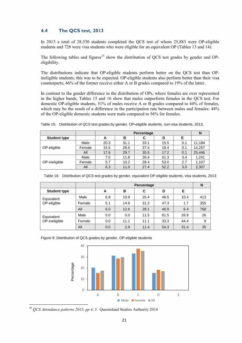
4.4 The QCS test, 2013 In 2013 a total of 28,530 students completed the QCS test of whom 25,883 were OP-eligible students and 728 were visa students who were eligible for an equivalent OP (Tables 13 and 14). The following tables and figures25 show the distribution of QCS test grades by gender and OP-eligibility. The distributions indicate that OP-eligible students perform better on the QCS test than OP-ineligible students; this was to be expected. OP-eligible students also perform better than their visa counterparts; 46% of the former receive either A or B grades compared to 19% of the latter. In contrast to the gender difference in the distribution of OPs, where females are over represented in the higher bands, Tables 15 and 16 show that males outperform females in the QCS test. For domestic OP-eligible students, 51% of males receive A or B grades compared to 44% of females, which may be the result of a difference in the participation rate between males and females: 44% of the OP-eligible domestic students were male compared to 56% for females.

Table 15: Distribution of QCS test grades by gender, OP-eligible students, non-visa students, 2013,

Percentage N

Student type A B C D E

OP-eligible Male 20.3 31.1 33.1 15.5 0.1 11,184

Female 15.5 28.6 37.4 18.4 0.1 14,257 All 17.6 29.7 35.5 17.2 0.1 25,446

OP-ineligible Male 7.0 11.8 26.4 51.3 3.4 1,241

Female 5.7 10.2 28.4 53.0 2.7 1,107 All 6.3 11.0 27.4 52.2 3.0 2,307

Table 16: Distribution of QCS test grades by gender, equivalent OP-eligible students, visa students, 2013

Percentage N

Student type A B C D E

Equivalent OP-eligible

Male 6.8 10.9 25.4 46.5 10.4 413 Female 5.1 14.6 31.3 47.3 1.7 355 All 6.0 12.6 28.1 46.9 6.4 768

Equivalent OP-ineligible

Male 0.0 0.0 11.5 61.5 26.9 26 Female 0.0 11.1 11.1 33.3 44.4 9 All 0.0 2.9 11.4 54.3 31.4 35

Figure 9: Distribution of QCS grades by gender, OP-eligible students

25 QCS Attendance patterns 2013, pp 4, 5. Queensland Studies Authority 2014

Per

cent

age

22

Figure 10: Distribution of QCS grades by gender, equivalent OP-eligible students

4.5 Relationship of QCS Test scores with grades and SAIs One of the requirements of a scaling test is that there is a strong relationship with the test being scaled. The following box plots show the relationship between QCS test scores and student grades in English in 2013. Figure 11: Relationship between QCS test scores and student grades in English, 2013

The boxplots indicate a strong linear relationship between median QCS test scores and grades awarded in English across schools. Some overlap of QCS test scores between levels of achievements is evident, which is to be expected, given the coarseness of the grades.

0

10

20

30

40

50

60

1 2 3 4 5Male Female All

P

erce

ntag

e

23

QCS test score: Mean = 163.0 Mean Difference = 26.8

SAI Mean = 282.1 Mean Difference = 65.2

Correlation = 0.760

100

120

140

160

180

200

220

240

200 250 300 350 400

140

160

180

200

220

240

260

200 250 300 350 400

100

120

140

160

180

200

220

200 250 300 350 400

Since the scaling test is also required to moderate or scale students’ SAIs in subject-groups within schools, there should also be a strong relationship between QCS test scores and SAIs within schools. The following figures illustrate the relationship between QCS tests scores and SAIs in English for three different schools. The particular school-groups differ both in size and in the range of QCS test scores.

Figure 12: Plot of SAIs in English against QCS test scores – school A (n = 47)

Figure 13: Plot of SAIs in English against QCS test scores – school B (n = 29)

Figure 14: Plot of SAIs in English against QCS test scores – school C (n = 17)

The scatter plots and correlations vary across the

three schools. The correlation is highest in the smallest school which has the largest range of both SAI scores and QCS test scores. The correlation between QCS test score and SAI is least for school B because of the small range of QCS test scores.

QCS

test

scor

e QCS test score:

Mean = 163.0 Mean Difference = 22.I

SIA: Mean = 290.4 Mean Difference = 39.9

Correlation = 0.585

QCS test score: Mean = 195.53 Mean Difference = 20.7

SIA: Mean = 277.6 Mean Difference = 45.5

Correlation = 0.419

QC

S re

st s

core

SAI

SAI

SAI

QC

S te

st s

core

SAI

24

What is evident from the data presented in this section is that, although there are relatively strong relationships between QCS scores, grades and SAIs, there is considerable scatter, which suggests that some of the QCS test scores may be anomalous. 5. CALCULATING SCALING SCORES 5.1 Introduction The previous chapter has shown that while the SAIs provide fine discrimination between students in their courses, unlike grades, they are not comparable across schools or across subjects-groups within schools. In order to make comparisons between students studying the same subject in different schools, or to compare the achievement of students in the different subjects-groups in the same school, the SAIs must be transformed so that they are on the same scale. The procedure used for this purpose is termed scaling. Linear transformations are used to change the SAIs of OP-eligible students into scaled SAIs that have the following two characteristics:

· The mean of the scaled SAIs of OP-eligible students in a subject-group is equal to the mean of the scaling scores of these students.

· The mean-difference of the scaled SAIs of OP-eligible students in a subject-group is equal to the mean-difference of these students.

The first step in this process is to determine a set of suitable scaling scores. Six scaling scores are derived from the QCS test item scores, one for the calculation of the OAIs and one for each of the five FAIs.

5.2. Scaling score for the OAIs OAIs provide a measure of students’ positions based on their overall academic achievements. The scaling score for the OAI is the unweighted sum of the QCS test item scores. 5.3 Scaling scores for the FAIs FAIs provide measures of students’ positions based on their achievements in the five fields. The scaling scores for the five fields are weighted sums of QCS test item scores, where the weights are indicative of the importance of the items for each of the five fields. For Field Position A, for example, the scaling score is related to skills necessary for complex analysis and synthesis of ideas in extended written expression. For Field Position C the scaling score is related to basic numeracy involving simple calculations and graphical investigations. The weights applied to the QCS test items are termed item field weights and are determined at the fielding meeting. 5.4 Calculating item field weights When determining the field weights that are used to construct the five field scaling scores two considerations are taken into account:

· Each scaling score should measure a single attribute related to one of the five fields so

should have high reliability as assessed by Cronbach’s alpha (α). The fielding committee has set the expectation that alpha should exceed 0.7 for each fielding score.

25

Field A Field B Field C Field D

· As the skills underpinning the five fields are distinct, the correlations between the five

scaling scores should be low. The committee has set the expectation that the correlations between the Fields A, B, C and D should not exceed 0.7, and that none should correlate more highly that 0.8 with the field E score.

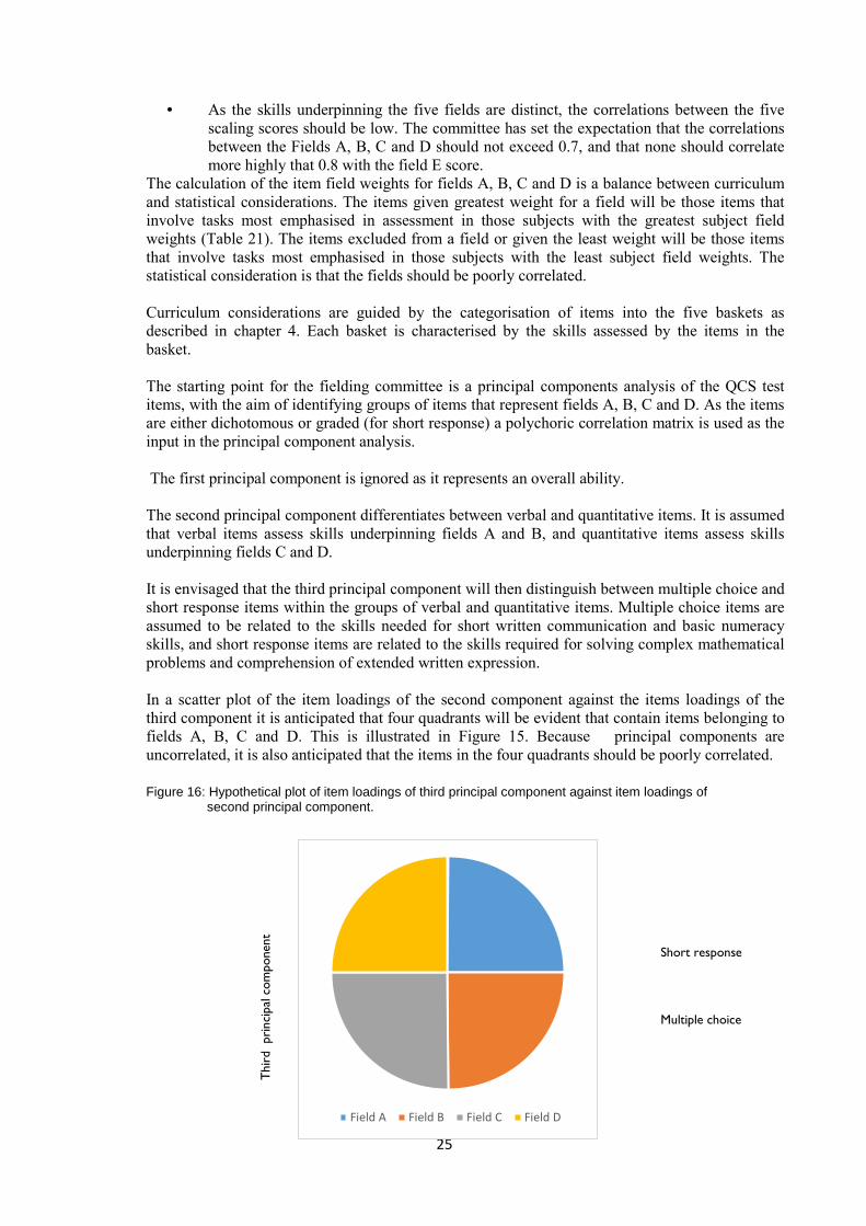
The calculation of the item field weights for fields A, B, C and D is a balance between curriculum and statistical considerations. The items given greatest weight for a field will be those items that involve tasks most emphasised in assessment in those subjects with the greatest subject field weights (Table 21). The items excluded from a field or given the least weight will be those items that involve tasks most emphasised in those subjects with the least subject field weights. The statistical consideration is that the fields should be poorly correlated. Curriculum considerations are guided by the categorisation of items into the five baskets as described in chapter 4. Each basket is characterised by the skills assessed by the items in the basket. The starting point for the fielding committee is a principal components analysis of the QCS test items, with the aim of identifying groups of items that represent fields A, B, C and D. As the items are either dichotomous or graded (for short response) a polychoric correlation matrix is used as the input in the principal component analysis. The first principal component is ignored as it represents an overall ability. The second principal component differentiates between verbal and quantitative items. It is assumed that verbal items assess skills underpinning fields A and B, and quantitative items assess skills underpinning fields C and D. It is envisaged that the third principal component will then distinguish between multiple choice and short response items within the groups of verbal and quantitative items. Multiple choice items are assumed to be related to the skills needed for short written communication and basic numeracy skills, and short response items are related to the skills required for solving complex mathematical problems and comprehension of extended written expression. In a scatter plot of the item loadings of the second component against the items loadings of the third component it is anticipated that four quadrants will be evident that contain items belonging to fields A, B, C and D. This is illustrated in Figure 15. Because principal components are uncorrelated, it is also anticipated that the items in the four quadrants should be poorly correlated. Figure 16: Hypothetical plot of item loadings of third principal component against item loadings of

second principal component. Short response Multiple choice

Thir

d p

rinc

ipal

com

pone

nt

26

Quantitative Verbal

Second principal component

The actual scatter plot from 2013 is not as clear. The scatter plot (Figure 17) shows a clear division between the quantitative and verbal items but the division between multiple choice and short response items is less clear, with the short response items scattered among the multiple choice items. Given the relatively small number of short response items and the high correlation between the item types (for the 2013 tests the correlation between multiple choice and short response items was 0.817) this is not surprising. The Writing Task, which could be expected to anchor the items pertaining to Field A is embedded in a cluster of multiple choice items. The pattern suggests that a two factor solution is more appropriate than a four factor solution. In the scatter plot of the third principle component loadings against the second principal component loadings the items are colour coded by type as shown below.

MC Q: Multiple Choice MC V: Multiple Choice SR Q: Short response SR V: Short response Quantitative Verbal Quantitative Verbal

Figure 1726: Scatter plot of third principal component loadings against second principal component

loadings

26 Queensland Core Skills Test 2013 QCS Yearbook, page 22.Queensland Studies Authority.

Third

prin

cipa

l com

pone

nt

27

The committee’s task is to examine the items in each quadrant and consider the nature of the items. Boundaries are drawn between areas that appear to define the four fields – A, B, C and D so that each item is allocated to a field. In making their judgements the committee makes use of the following extended descriptions of the fields that allow multiple choice items to provide evidence for Fields A and D.

A extended written expression involving complex analysis and synthesis of ideas or elements of writing necessary to complete such tasks

B short written communication involving reading, comprehension and expression in English or a foreign language or understanding the elements necessary to complete such tasks

C basic numeracy involving simple calculations and graphical, diagrammatic and tabular and scientific interpretation

D solving complex problems involving mathematical symbols and abstractions or elements of problem solving necessary to complete such tasks, including complex graphical and scientific interpretation

E substantial practical performance involving physical and creative arts or expressive skills

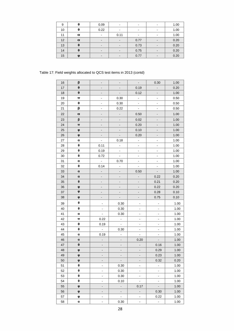
Multiple choice items that are allocated to one of the fields A, B, C or D will have a non-zero field weight corresponding to that field and zero weights for the remaining fields. The non-zero field weight is calculated by the length of the projection of the position of the item on to the line that bisects the boundaries. Field weights for items on Field E are determined by the nature of the items. All items are given an initial weight of 1, and items that require skills associated with practical components such as performance are identified and given higher weights. Consequently all items load on field E but only a small number of units having items with large weights. The allocations are checked and modifications made if necessary. Curriculum considerations are allowed to override statistical considerations and items can be assigned to more than one field if the committee concludes that such modifications are warranted. The following table (Table 17) shows the allocation of item types to fields in the 2013 QCS test, the corresponding item field weights and the baskets to which the items belong. Examination of the scatter plot and the resulting field weights indicates that curriculum considerations have played a substantial role in the allocation decisions, which is consistent with the committee’s function.

Table 1727: Field weights allocated to QCS test items in 2013

Item Basket Field A Field B Field C Field D Field E

1 α - 0.30 - - 1.00

2 θ - - - 0.60 1.00

3 α - - - 0.26 1.00

4 θ 0.03 - - - 1.00

5 α 0.13 - - - 1.00

6 θ - 0.14 - - 0.20

7 θ - 0.15 - - 0.20

8 α - 0.30 - - 0.20

27 Queensland Core Skills Test 2013 QCS Yearbook, page 23. Queensland Studies Authority

Second principal component

28

9 θ 0.09 - - - 1.00

10 θ 0.22 - - - 1.00

11 α - 0.11 - - 1.00

12 α - - 0.77 - 0.20

13 θ - - 0.73 - 0.20

14 θ - - 0.75 - 0.20 15 φ - - 0.77 - 0.20

Table 17: Field weights allocated to QCS test items in 2013 (contd)

16 β - - - 0.30 1.00 17 θ - - 0.19 - 0.20

18 θ - - 0.12 - 1.00

19 π - 0.30 - - 0.50

20 θ - 0.30 - - 0.50

21 β - 0.22 - - 0.50

22 α - - 0.50 - 1.00

23 β - - 0.02 - 1.00

24 π - - 0.20 - 1.00

25 φ - - 0.10 - 1.00

26 φ - - 0.20 - 1.00

27 α - 0.18 - - 1.00

28 θ 0.11 - - - 1.00

29 θ 0.19 - - - 1.00

30 θ 0.72 - - - 1.00

31 α - 0.70 - - 1.00

32 θ 0.14 - - - 1.00

33 α - - 0.50 - 1.00

34 α - - - 0.22 0.20

35 θ - - - 0.21 0.20

36 φ - - - 0.22 0.20

37 φ φ

- - - 0.28 0.10

38 φ - - - 0.75 0.10

39 θ - 0.30 - - 1.00

40 θ - 0.30 - - 1.00

41 α - 0.30 - - 1.00

42 π 0.22 - - - 1.00

43 θ 0.19 - - - 1.00

44 θ - 0.30 - - 1.00

45 α 0.19 - - - 1.00

46 α - - 0.20 - 1.00

47 θ - - - 0.16 1.00

48 φ - - - 0.29 1.00

49 φ - - - 0.23 1.00

50 φ - - - 0.32 0.20

51 θ - 0.30 - - 1.00

52 θ - 0.30 - - 1.00

53 θ - 0.30 - - 1.00

54 θ - 0.10 - - 1.00

55 φ - - 0.17 - 1.00

56 φ - - - 0.30 1.00

57 φ - - - 0.22 1.00

58 α - 0.30 - - 1.00

29

59 θ - 0.30 - - 1.00 60 θ - 0.30 - - 1.00 61 α 0.14 - - - 1.00 62 θ - 0.17 - - 1.00 63 α - - 0.20 - 1.00 64 φ - - 0.02 - 1.00 65 φ - - 0.20 - 1.00 66 θ - - - 0.28 1.00 67 θ - 0.30 - - 1.00

Table 17: Field weights allocated to QCS test items in 2013 (contd).

68 β - 0.30 - - 1.00 69 β - 0.30 - - 1.00 70 π - 0.30 - - 1.00 71 θ 0.22 - - - 1.00 72 θ 0.22 - - - 1.00 73 α - - 0.05 - 1.00 74 β - - - 0.30 1.00 75 β - - 0.20 - 1.00 76 β - - - 0.20 1.00 77 θ - - - 0.77 0.20 78 β - - - 0.26 1.00 79 θ - 0.19 - - 2.00 80 β - 0.12 - - 2.00 81 α - 0.30 - - 2.00 82 β - 0.30 - - 2.00 83 α - 0.30 - - 2.00 84 α - - - 0.29 0.20 85 θ - - - 0.29 1.00 86 φ - - - 0.25 1.00 87 α - - - 0.27 1.00 88 α - - - 0.18 1.00 89 α - - - 0.24 1.00 90 α - - - 0.20 1.00 91 θ 0.12 - - - 1.00 92 θ - 0.70 - - 1.00 93 α 0.18 - - - 1.00 94 θ 0.20 - - - 1.00 95 θ 0.23 - - - 1.00 96 β - - 0.02 - 3.00 97 θ - - 0.40 - 2.00 98 β - - 0.01 - 3.00 99 β

- - - 0.16 3.00

100 β

- - - 0.28 3.00

In the above table the groups of shaded rows represent stimulus units. Within most units the majority of items come from one basket.

Table 18 shows the spread of the different types of items across the fields. While the sets of items loading on fields A to D are disjoint, all items load on Field E.

Table 18: Distribution of types of items across fields A, B, C, D and E

Item type A B C D E

30

Multiple choice 18 32 22 28 100

Short Response 5 4 8 2 19

Writing task 1 1

Table 19 shows the relationship between baskets and field items. Comprehension items are spread across all fields, items focused on analysis and drawing conclusions tend to be concentrated in fields A and B, and items related to applying techniques and procedures limited to fields C and D. Table 19: Distributions of items by basket and field

Field Basket Total

α β θ π φ A 4 0 13 1 0 18 B 9 5 16 2 0 32 C 5 5 5 1 6 22 D 9 5 5 0 9 28

The descriptive statistics and frequency histograms of the item weights are shown below. Table 20: Descriptive statistics of item weights by field

Field N Min Max Mean Mean Difference

A 18 0.03 0.72 0.197 0.142 B 32 0.10 0.70 0.284 0.129 C 22 0.01 0.77 0.287 0.264 D 28 0.16 0.77 0.297 0.153 E 100 0.10 3.00 0.995 0.580

Figures 18-22: Histograms of item weights for fields A to E

Field A Field B Field C

Field D Field E

31

The patterns of item weights are similar for fields A, C and D, with most item weights spread cross a narrow band of values and a small number of outliers. In contrast, the weights for field B are more concentrated around one value, with a small number of outliers on either side. The distribution of item weights for field E shows that only a very small number of items are related to substantial practical performance involving physical and creative arts or expressive skills. The remaining field weights were assigned a value of 1 so that there will be some variation in the scaling scores for Field E but, in so doing, the resulting scaling score may not have high face validity. It is closer to a measure of overall ability rather than a measure of practical performance, which is borne out from an examination of the correlations between the scaling scores. 5.5 Calculating scaling scores Students’ scaling scores are calculated by applying the item field weights to the QCS test item scores and aggregating the weighted item scores as sown below. Six scaling scores are calculated; one that is used in the determination of students’ OPs and the remaining five that are used in the determination of the five FPs. Scaling score = ∑wj xj where xj is the score of the jth item wj is the item field weight of the jth item

The purpose of fielding was to construct scaling scores that are appropriate for scaling SAIs to be used to calculate students’ OIAs and FAIs that would be the basis of the calculation of the five field positions. Table 21 shows the correlations between the scaling scores derived in 2013. Table 21: Correlations between scaling scores, 201328

A B C D E QCS test A 1.000 0.724 0.449 0.483 0.756 0.848 B 0.724 1.000 0.472 0.496 0.773 0.785

C 0.449 0.472 1.000 0.682 0.775 0.752

D 0.483 0.496 0.682 1.000 0.764 0.784

E 0.756 0.773 0.764 0.764 1.000 0.955

QCS test 0.848 0.785 0.726 0.784 0.955 1.000

The pattern of correlations observed in 2013 is very similar to that seen in previous years and is what would be expected for fields A, B, C and D. The scaling scores for the two verbal fields (A and B) are highly correlated, as are the scaling scores for the two quantitative fields (C and D). The scaling scores for the quantitative fields are more highly correlated than those for the verbal fields, which is not unusual. The correlations between the verbal and quantitative scaling scores are moderate, approximately 0.5. Since the item scores that make up each field score are contained in the QCS test total score, the correlations of the field scaling scores with the QCS test total score are high and relatively uniform. As would be expected from the field weights, the scaling score for field E is very highly correlated (r = 0.955) with the QCS total test score. 5.6 Discussion

28 Queensland Core Skills Test. 2013 Yearbook, page 26.

32

Fielding is an essential part of the scaling process because of the importance placed on field positions but the data presented above raise questions about their role. The principal components analysis and the correlations between the scaling scores suggest strongly that only two components, verbal and quantitative, are required. The short response and multiple choice items are highly correlated, which is not unusual either for scaling tests or achievement tests. The pattern of item weights for Field E ensures that the scaling score for Field E is highly correlated with the other four scaling scores and resembles closely a measure of overall ability. Field positions were given an important role in the tertiary admission process when the current structure was introduced in 1990. Given the complexity of the fielding process and the changes that have occurred in the tertiary admission procedures, perhaps it is time to re-think their role. 6. FIRST STAGE SCALING: COMPARING SUBJECT- GROUPS

WITHIN SCHOOLS

6.1 Overview The purpose of this phase is to scale the SAIs to make them comparable across subject-groups in the same school to make it possible to compare the achievements of students in one subject-group in a school with the achievement of students in another subject-group in the same school. The previous chapter has described the calculation of the six scaling scores used in the scaling process. A second measure of overall academic achievement, the Within School Measure (WSM) is derived directly from paired comparisons of students’ SAIs. This measure is used to detect anomalous performance of students on the QCS test. The SAIs of a subject-group within a school are scaled by linear scaling, using the scaling scores derived from the QCS test scores for OP-eligible students, which ensures that the relativities of SAIs within a subject-group remain unchanged. Scaled SAIs will have the same mean and mean-difference of the QCS test scaling scores for that subject-group, with isoweights being applied to the scaling scores of individual students. These weights take into account the relationship between the scaling score and the WSM and are used to reduce the influence of anomalous performance on the QCS test on the calculation of the scaling parameters for the subject-groups in the school. Following the scaling of the SAIs up to six composite measures are calculated for each OP-eligible student. For each OP-eligible student an Overall Achievement Indicator (OAI) is determined by averaging the best scaled SAIs of 20 semester units of credit in Authority subjects, including at least three subjects studied for four semesters. The OAI reflects the relative placement of a student within a school-group based on overall performance. The scaling score is the used in the calculation of the scaling parameters for each subject-group is the unweighted aggregate of the QCS Test item scores. A similar process is used to calculate the following five Field Achievement Indicators (FAIs):

Field Achievement Indicator –Field A (FAI –A) Field Achievement Indicator –Field B (FAI –B) Field Achievement Indicator –Field C (FAI –C) Field Achievement Indicator –Field D (FAI –D) Field Achievement Indicator –Field E (FAI –E)

In the calculation of a Field Achievement Indicator the first step is to scale the SAIs of eligible students using the appropriate scaling score with isoweights applied to students’ scaling scores.

33

0

1

2

3

4

5

6

200 239 259 265 271 278 287 292 299 312 318 323 341 343 367 400

Subject weights, which indicate the importance of Authority subjects to the specific field, are then applied to the scaled SAIs before they are aggregated. 6.2 Linear scaling The linear equation used to scale the SAIs has the form

Y = μ + (σ/s) (X – m) where

· X is the SAI being scaled · m and s are the location and scale parameters, the weighted mean and mean difference

respectively, of the SAIs · μ and σ are the location and scale parameters, the mean and mean difference

respectively, of the relevant scaling score. The location and scale parameters, which are the weighted mean and mean difference of the scaling scores are termed the subject-group’s scaling parameters. A linear transformation changes the mean and mean difference of the SAIs so that the scaled SAIs have mean μ and mean difference σ. The relativities between the SAIs, however, are preserved. 6.3 Calculating the location and scale parameters of the SAI scores of

large subject-groups The location and scale parameters of the SAIs are the weighted mean and mean difference of the SAI scores of OP-eligible students in the subject-group. In the calculation of the mean and mean difference students’ SAIs are weighted by the number of semester units completed in the subject, which reflect the students’ loads associated with the subject. The mean of the SAIs of the English subject-group in School A (Section 4.5) was 290.4 and the mean difference was 39.9. The SAIs were distributed between 200 and 400 as shown in the following figure. Figure 23 Frequency histogram of SAIs for English subject-group, School A

6.4 Calculating the scaling score parameters of the SAI scores in large subject-groups

The first step in the calculation of the scaling score parameters is the distribution of the scaling scores for the subject-group. Figure 24 shows the histogram of the QCS test scores, which are the scaling scores for the OAIs, for the large English subject-group described in the previous section.

Freq

uenc

y

SAI

34

200 250 300 350 400

These scores are distributed between 113 and 221, with mean score of 181.0 and mean difference 22.57. Figure 24: Histogram of QCS test scores for the English Subject-group, School A

SAI

The second step is to examine the relationship between QCS total tests scores and the SAIs for the subject-group to determine if there are any anomalous QCS scores. The following figures shows the scatter plot of QCS scores against SAI scores. Figure 25: Scatter plot of QCS test score against SAI

.

The relationship between the two sets of scores is relatively strong (r = 0.585) but there is considerable scatter which suggests that some QCS scores may be anomalous. Rather than disregarding anomalous scaling scores, the QSA determines weights to be applied to student’s QCS scores so that anomalous scores are down-weighted. This reduces their effect on the calculation of the scaling parameters. These weights are termed isoweights. 6.5 Determining isoweights

Isoweights are determined from an analysis of the relationship between students’ ranking as determined by their SAIs and a non-parametric measure of their overall achievement based on paired comparisons between students. This measure is termed the Within School Measure29 (WSM). Students whose ranking on the basis of the QCS Test scaling score is significantly different from their ranking on the WSM will have their scores down-weighted.

29 David, H. A. (1987) Ranking from unbalanced paired-comparison data. Biometrika, 74, 2, pp432-436

0

1

1

2

2

3

3

4

113 144 152 160

SAI

QCS

test

scor

e

Freq

uenc

y

240 200 160 100

35

Q

CS

test

tota

l sco

res

-40

-30

-20

-10

0

10

20

30

40

120 140 160 180 200 220 240

The calculation of WSMs for OP-eligible students consists of comparing the subject achievements of students in the school-group, keeping account of the number of times a student “wins” or “loses” these comparisons30. In summary,

· compare each student with every other student who has a subject in common · turn SAIs into preferences: wins, losses, draws · assign a weight to each preference · add the (weighted) wins of this student (W1) · add the total (weighted) wins of persons beaten by this student (W2) · add the (weighted losses of this student (L1) · add the total (weighted) losses of persons this student lost to (L2)

WSM = all wins – all losses = (W1 + W2) – (L1 + L2) The distributions of WSMs in large school-groups are first transformed so that they have the same mean and mean difference as the school-group’s distribution of QCS scores for OP-eligible students. This is done by finding the unweighted mean and mean difference of WSMs and QCS test scores and rescaling the WSMs by a linear transformation. The second step is to plot students’ QCS test scores against their WSMs and determine the distances between their QCS test scores and the value predicted by their WSMs, as shown in the following figure. Figure 26 Scatter plot of QCS test scores on WSM for school-group A (n = 47)

WSM

For each point the perpendicular distance from the model line is then calculated and plotted as shown in the following figure. The two blue lines are one mean-difference above and below the model line. The distribution of the points suggest that there may be a small number of anomalous QCS test results. Figure 27: Plot of perpendicular distances from the model line for school A (n = 47)

30 A full description of the calculation of the WSM is found in the QSA document Guideline for determining Overall Positons (OPs) and Field Positions (FPs), October 2012, pp12-14.

100

120

140

160

180

200

220

240

100

Diff

eren

ce

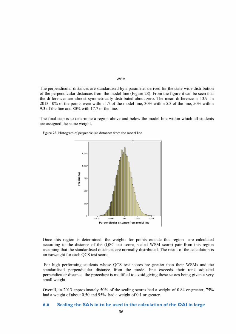
36

WSM

The perpendicular distances are standardised by a parameter derived for the state-wide distribution of the perpendicular distances from the model line (Figure 28). From the figure it can be seen that the differences are almost symmetrically distributed about zero. The mean difference is 13.9. In 2013 10% of the points were within 1.7 of the model line, 30% within 5.3 of the line, 50% within 9.3 of the line and 80% with 17.7 of the line. The final step is to determine a region above and below the model line within which all students are assigned the same weight.

Figure 28 Histogram of perpendicular distances from the model line Once this region is determined, the weights for points outside this region are calculated according to the distance of the (QSC test score, scaled WSM score) pair from this region assuming that the standardised distances are normally distributed. The result of the calculation is an isoweight for each QCS test score. For high performing students whose QCS test scores are greater than their WSMs and the standardised perpendicular distance from the model line exceeds their rank adjusted perpendicular distance, the procedure is modified to avoid giving these scores being given a very small weight. Overall, in 2013 approximately 50% of the scaling scores had a weight of 0.84 or greater, 75% had a weight of about 0.50 and 95% had a weight of 0.1 or greater. 6.6 Scaling the SAIs in to be used in the calculation of the OAI in large

37

0

1

2

3

4

5

6

130 152 163 167 170 174 179 185 187 195 200 210 219 230

subject-groups The first step is to apply the isoweights to students’ scaling scores. For large subject-groups the weighted mean31 (μ) and weighted mean-difference (σ) the scaling scores in this case the QCS tests total scores) are calculated for the subject-group. These are the scaling parameters of the subject group. The SAIs are scaled using the linear equation shown in section 6.2. The result of scaling is that the spread of the scaled SAIs is similar to that of the scaling scores with a mean of 181 and range from 113 to 243. The form of the distribution, however, resembles that of the original SAIs than that of the QCS tests scores. The relativities between students have been preserved. Figure 29: Histogram of scaled SAIs for English subject-group (n=47)

6.7 Scaling SAIs for students in small and intermediate subject-groups within schools

The above method is only used for large subject-groups. For small subject-groups, with less than ten OP-eligible students, the scaling parameters are based on information from large subject-groups in that subject. For all large subject-groups in the subject across the state, the scaled SAI grade boundary values are determined and averaged. These boundary values are then used for the small subject-groups’ level SAIs, and the rung SAIs found by interpolation32. The following tables illustrate the procedure. The first table shows the average boundary scaled SAIs of all English large-subject groups. Table 22: Average boundary scaled SAIs of all large subject-groups

Grade boundary Scaled SAI boundary

VHA/HA 330

31 The formulae for the weighted mean and weighted mean difference can be found on page 12 Guideline for determining Overall Positions (OPs) and Field Positions (FPs). Queensland Studies Authority, November 2012. 32 Guideline for determining Overall Positions (OPs) and Field Positions (FPs),page 15. Queensland Studies Authority, November 2012

Fr

eque

ncy

38

HA/SA 260 SA/LA 226

The second table (Table 23) shows the scaled SAIs in a small English subject-group of three students whose SAIs are H rung 2, SA rung 5 and LA rung 6. From Table 19 it is seen that SAI H rung 2 lies between 260 and 330. Linear interpolation gives a scaled SAI of 274. Table 23: Scaled SAIs in a small English subject-group

Grade Rung SAI Scaled SAI

H 2 274 S 5 243

L 6 204

SAIs for intermediate subject-groups, with 10 to 13 OP-eligible students, are scaled by both the small subject-group and large subject-group method. A weighted average of the two values is calculated, with the weight for the large group model increasing from 20% for 10 students to 30% for 13 students, which ensures a smooth transition from the large-group model to the small-group model. 6.8 Scaling SAIs to be used in the calculation of FAIs The above procedure is applied to each field position (FP - A, FP - B, FP - C, FP - D, FP - E) for which students are eligible. In summary:

· For each student scaling scores are calculated for the fields for which the student is eligible using the field weights determined by the fielding committee

· WSMs are determined for students who are eligible for that field position · The relationships between scaling scores and WSMs are examined for each subject-

group, and isoweights are calculated as described above. · The scaling parameters are found for relevant large subject-groups in the school · The SAIs of eligible students are scaled by linear transformations

6.9 Visa students Queensland is unique in the way that the results of visa students are treated. They are removed from the calculation of the scaling parameters of subject-groups on the assumption that any deficiency in English language proficiency would result in scores on the QCS Test that do not reflect their ability. Lower QCS test scores would affect not only their own scaling score but would have an effect on the scaling parameters of the subject-group and school-group to which they belong. The SAIs of these visa students are scaled using the subject-group scaling parameters based on the non-visa students in the subject-group33. The strategy adopted for visa subject-groups, which have a relatively large proportion of visa students, is similar to a regression approach to estimating “true scores” from “observed scores”.

33 Guideline for determining Overall Positions (OPs) and Field Positions (FPs), pages16-17. Queensland Studies Authority, November 2012

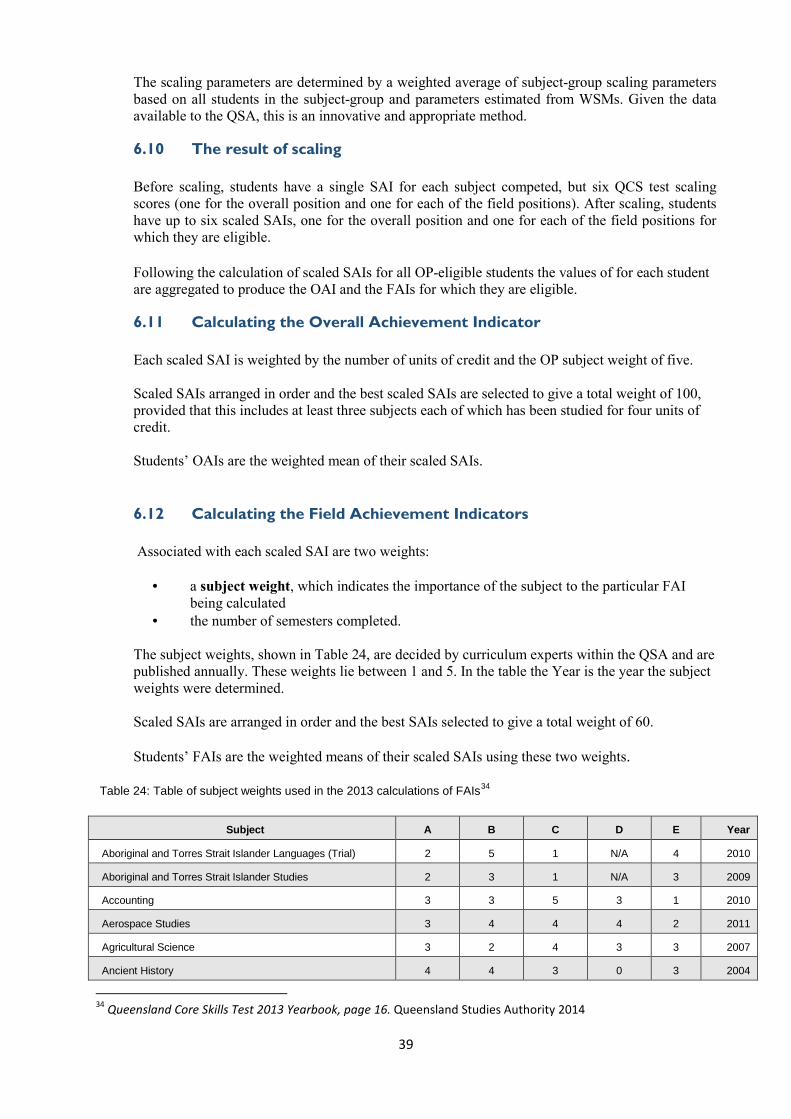
39

The scaling parameters are determined by a weighted average of subject-group scaling parameters based on all students in the subject-group and parameters estimated from WSMs. Given the data available to the QSA, this is an innovative and appropriate method. 6.10 The result of scaling Before scaling, students have a single SAI for each subject competed, but six QCS test scaling scores (one for the overall position and one for each of the field positions). After scaling, students have up to six scaled SAIs, one for the overall position and one for each of the field positions for which they are eligible. Following the calculation of scaled SAIs for all OP-eligible students the values of for each student are aggregated to produce the OAI and the FAIs for which they are eligible. 6.11 Calculating the Overall Achievement Indicator Each scaled SAI is weighted by the number of units of credit and the OP subject weight of five. Scaled SAIs arranged in order and the best scaled SAIs are selected to give a total weight of 100, provided that this includes at least three subjects each of which has been studied for four units of credit. Students’ OAIs are the weighted mean of their scaled SAIs. 6.12 Calculating the Field Achievement Indicators Associated with each scaled SAI are two weights:

· a subject weight, which indicates the importance of the subject to the particular FAI being calculated

· the number of semesters completed. The subject weights, shown in Table 24, are decided by curriculum experts within the QSA and are published annually. These weights lie between 1 and 5. In the table the Year is the year the subject weights were determined. Scaled SAIs are arranged in order and the best SAIs selected to give a total weight of 60. Students’ FAIs are the weighted means of their scaled SAIs using these two weights.

Table 24: Table of subject weights used in the 2013 calculations of FAIs34

Subject A B C D E Year

Aboriginal and Torres Strait Islander Languages (Trial) 2 5 1 N/A 4 2010

Aboriginal and Torres Strait Islander Studies 2 3 1 N/A 3 2009

Accounting 3 3 5 3 1 2010

Aerospace Studies 3 4 4 4 2 2011

Agricultural Science 3 2 4 3 3 2007

Ancient History 4 4 3 0 3 2004

34 Queensland Core Skills Test 2013 Yearbook, page 16. Queensland Studies Authority 2014

40

Biology 5 4 4 3 2 2004

Business Communication and Technologies 3 3 4 3 3 2008

Business Organisation and Management 3 3 4 3 3 2007

Chemistry 4 3 5 5 2 2007

Chinese 1 5 1 N/A 3 2008

Chinese Extension (Trial) 2 5 1 N/A 4 2010

Dance 2 1 1 N/A 5 2010

Drama 3 2 1 N/A 5 2007

Earth Science 3 3 4 3 2 2000

Economics 5 5 4 3 1 2010

Engineering Technology 3 2 5 5 3 2010

English 5 4 1 N/A 3 2010

English Extension (Open Trial) 5 2 1 N/A 2 2010

English for ESL Learners (extended trial) 3 4 1 N/A 3 2007

Film, Television and New Media 3 2 2 N/A 5 2005

French 1 5 1 N/A 3 2008

French Extension 2 5 1 N/A 4 2009

Table 25: Table of subject weights used in the 2013 calculations of FAIs (contd)

Geography 4 5 4 3 2 2007

German 1 5 1 N/A 3 2008

German Extension 2 5 1 N/A 4 2009

Graphics 1 2 5 3 4 2007

Health Education 5 2 3 2 2 2010

Home Economics 3 4 3 2 4 2010

Hospitality Studies 2 3 3 2 4 2009

Indonesian 1 5 1 N/A 3 2008

Indonesian Extension 2 5 1 N/A 4 2009

Information Processing and Technology 3 2 4 4 3 2010

Information Technology Systems

3 2 3 3 3 2006

Italian 1 5 1 N/A 3 2008

Japanese 1 5 1 N/A 3 2008

Korean 1 5 1 N/A 3 2008

Latin 2 5 1 N/A 2 2008

Legal Studies 5 4 2 1 2 2007

Marine Studies 2 3 4 3 3 2004

Mathematics A 1 2 5 4 N/A 2008

Mathematics B 1 2 5 5 N/A 2008

Mathematics C 1 2 5 5 N/A 2008

Modern Greek 1 5 1 N/A 3 2008

41

Modern History 5 4 2 N/A 3 2004

Music 2 1 2 1 5 2004

Music Extension 3 1 2 2 5 2008

Philosophy and Reason 5 4 3 3 1 2004

Physical Education 3 1 3 2 5 2010

Physics 4 3 5 5 2 2007

Polish 1 5 1 N/A 3 2008

Russian 1 5 1 N/A 3 2008

Science21 4 4 5 4 2 2010

Spanish 1 5 1 N/A 3 2008

Study of Religion 5 4 2 N/A 2 2008

Study of Society 5 4 3 2 2 2001

Technology Studies 2 1 4 3 4 2007

Vietnamese 1 5 1 N/A 3 2008

Visual Art 4 2 2 N/A 5 2007

The pattern of weights show that written expression and basic mathematical skills are regarded as having some relevance for all subjects but complex mathematical skills are deemed unimportant for many areas. Practical and creative skills are regarded as important for most subjects but not all.

6.13 Relationship between OAIs and FAIs Because the items included in the scaling scores for the field positions are also included in the scaling score for the overall position it is to expected that there will be some correlation between the six aggregate scores. The following table presents data on the QCS test total scores, WSMs, OAIs and FAIs for a large school group (n=52). Table 25: Correlations between OAIs and FAIs for a large school-group (n=52) in 2013

QCS test total score WSM OAI FAI-FA FAI-FB FAI-FC FAI-FD FAI-FE

QCS test total score 1.000 0.701 0.756 0.728 0.714 0.779 0.827 0.504

WSM 0.701 1.000 0.983 0.959 0.957 0.959 0.959 0.982

OAI 0.756 0.983 1.000 0.968 0.974 0.975 0.981 0.983

FAI-A 0.728 0.959 0.968 1.000 0.961 0.925 0.945 0.925

FAI-B 0.714 0.957 0.974 0.961 1.000 0.913 0.954 0.923

FAI-C 0.779 0.959 0.975 0.925 0.913 1.000 0.995 0.954

FAI-D 0.827 0.959 0.981 0.945 0.954 0.995 1.000 0.997

FAI-E 0.504 0.982 0.983 0.925 0.923 0.954 0.997 1.000

Because the OAIs are measures of overall achievement based on SAIs that have been scaled using the QCS test scores and validated against the WSMs, which are also measures of overall performance within a school-group, it is not surprising that the WSMs, QSC test scores and OAIs are strongly related. The correlation between OAIs and WSMs is very high, 0.983, and the others exceed 0.701. The correlations between the OAI and the FAIs and between the FAIs are also very high, with all exceeding 0.95.

42

These findings support the inference made earlier on the basis of the correlations between the scaling scores that, while the fields are designed to measure specific skills, they are all strongly related to overall achievement. Because the OAIs and FAIs are based on SAIs which a indicators of achievement, they are more strongly related to WSMs than with the QCS test scores.

6.15 Result of the first stage of scaling During the first stage of scaling, students were assigned up to six scaling scores: one for overall position and one for each field position for which they are eligible. These scaling scores are then used to scale SAIs from which the OAI and FAIs are derived. At the end of stage one, students have up to six within-school rankings; one based on their overall performance and the remaining rankings on their performance in the fields for which they are eligible.

43

7. SECOND STAGE SCALING: SCALING BETWEEN SCHOOLS

7.1 Overview The first stage of scaling places the OAIs and FAIs on the same scale as the scaling scores derived from the QCS test. It would therefore be expected that the measures would be comparable across schools. It is possible, however, that there may be some inflation in schools’ mean OAIs resulting from students’ OAIs being based on their best 20 units rather than on all their subjects. The amount of expansion or contraction of the mean differences will depend on the correlations between the subject-groups SAIs within schools. Stage two of the scaling process adjusts the OAIs of school groups to take account of differences that may have arisen and to ensure that the OAIs are comparable across schools. For large school groups the OAIs are scaled so that the means and mean differences of the rescaled OAIs are equal to the means and mean differences of the QCS test scores of the school groups. A linear transformation is then applied to adjust the means and mean differences of the schools’ OAIs but which leaves the relativities between students in the same school-group unaltered. The OAIs of small school-groups are not rescaled. The scaling parameters for the OAIs of intermediate school-groups are the weighted scaling parameters determined by applying the large group model and those determined by applying the small group model. The weights are chosen to provide a smooth transition from small to large schools, as described in the previous chapter. The result of the second stage scaling is that the OAIs from different schools are on the same scale, with relativities between schools determined by their mean QCS test scores. FAIs are not rescaled. 7.2 Distribution of OAIs and FAIs in 2013 With the exception of FAI-FPE the distributions of students’ OAIs and FAIs have similar spreads (Table 26) and all have a slight skew similar to that of OAI (Figure 30). Table 26: Descriptive statistics of students’ OAI, FAIs and QCS test scores, 2013

N Mean Std.

Deviation

QCS 24,663 175.3 24.9

OAI 25,082 175.3 24.5

FAI-FPA 23,762 179.9 21.9

FAI-FPB 20,284 180.6 21.5

FAI-FPC 21,219 181.0 21.8

FAI-FPD 9,007 191.0 22.4

FAI-FPE 8,639 173.6 19.7

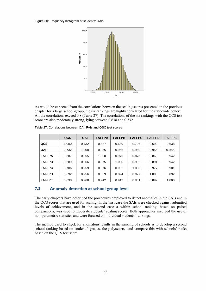
44

Figure 30: Frequency histogram of students’ OAIs

As would be expected from the correlations between the scaling scores presented in the previous chapter for a large school-group, the six rankings are highly correlated for the state-wide cohort. All the correlations exceed 0.8 (Table 27). The correlations of the six rankings with the QCS test score are also moderately strong, lying between 0.638 and 0.732. Table 27: Correlations between OAI, FAIs and QSC test scores

QCS OAI FAI-FPA FAI-FPB FAI-FPC FAI-FPD FAI-FPE

QCS 1.000 0.732 0.687 0.689 0.706 0.692 0.638

OAI 0.732 1.000 0.955 0.966 0.959 0.956 0.968.

FAI-FPA 0.687 0.955 1.000 0.975 0.876 0.869 0.942

FAI-FPB 0.689 0.966 0.975 1.000 0.902 0.894 0.942

FAI-FPC 0.706 0.959 0.876 0.902 1.000 0.977 0.901

FAI-FPD 0.692 0.956 0.869 0.894 0.977 1.000 0.892

FAI-FPE 0.638 0.968 0.942 0.942 0.901 0.892 1.000 7.3 Anomaly detection at school-group level The early chapters have described the procedures employed to detect anomalies in the SAIs and in the QCS scores that are used for scaling. In the first case the SAIs were checked against submitted levels of achievement, and in the second case a within school ranking, based on paired comparisons, was used to moderate students’ scaling scores. Both approaches involved the use of non-parametric statistics and were focused on individual students’ rankings. The method used to check for anomalous results in the ranking of schools is to develop a second school ranking based on students’ grades, the polyscore, and compare this with schools’ ranks based on the QCS test score.

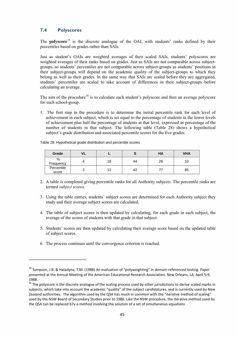
45

7.4 Polyscores The polyscore35 is the discrete analogue of the OAI, with students’ ranks defined by their percentiles based on grades rather than SAIs. Just as student’s OAIs are weighted averages of their scaled SAIs, students’ polyscores are weighted averages of their ranks based on grades. Just as SAIs are not comparable across subject-groups, so students’ percentiles are not comparable across subject-groups as students’ positions in their subject-groups will depend on the academic quality of the subject-groups to which they belong as well as their grades. In the same way that SAIs are scaled before they are aggregated, students’ percentiles are scaled to take account of differences in their subject-groups before calculating an average. The aim of the procedure36 is to calculate each student’s polyscore and then an average polyscore for each school-group. 1. The first step in the procedure is to determine the initial percentile rank for each level of

achievement in each subject, which is set equal to the percentage of students in the lower levels of achievement plus half the percentage of students at that level, expressed as percentage of the number of students in that subject. The following table (Table 28) shows a hypothetical subject’s grade distribution and associated percentile scores for the five grades.

Table 28: Hypothetical grade distribution and percentile scores

Grade VL L S HA VHA

% Frequency 4 16 44 26 10

Percentile score 2 12 42 77 95

2. A table is completed giving percentile ranks for all Authority subjects. The percentile ranks are

termed subject scores.

3. Using the table entries, students’ subject scores are determined for each Authority subject they study and their average subject scores are calculated.

4. The table of subject scores is then updated by calculating, for each grade in each subject, the

average of the scores of students with that grade in that subject. 5. Students’ scores are then updated by calculating their average score based on the updated table

of subject scores. 6. The process continues until the convergence criterion is reached.

35 Sympson, J.B. & Haladyna, T.M. (1988) An evaluation of “polyweighting” in domain-referenced testing. Paper presented at the Annual Meeting of the American Educational Research Association. New Orleans, LA, April 5-9, 1988. 36 The polyscore is the discrete analogue of the scaling process used by other jurisdictions to derive scaled marks in subjects, which take into account the academic “quality” of the subject candidatures, and is currently used by New Zealand authorities. The algorithm used by the QSA has much in common with the “iterative method of scaling” used by the NSW Board of Secondary Studies prior to 1986. Like the NSW procedure, the iterative method used by the QSA can be replaced b7y a method involving the solution of a set of simultaneous equations

46

50

100

150

200

250

300

50 100 150 200 250 300

7. Students’ scores are transformed so that they are normally distributed and scaled so that their mean and mean difference are the same as those of the scaled OAIs for OP-eligible students.

8. Students’ transformed scores are termed polyscores.

The result of these calculations is that the scaled OAIs and polyscores will have the same mean and mean difference as the QCS test scores. 7.5 Detecting anomalous schools Both OAI and polyscores are measures of students’ overall achievement, the first based on SAIs and the second on grades. A measure of the adequacy of the scaling of the OAIs is the strength of the relationship between the two measures. In 2013 the correlation between students’ OAIs and their polyscores was 0.948. Although the correlation was high, the scatter plot of students’ rescaled OAIs against their polyscores (Figure 31) shows some variability, which is not surprising given that polyscores are based on grades that are much coarser measures of achievement. There is, however, no evidence that of bias in the distribution of differences between OAIs and what are predicted from the polyscores. The histogram of perpendicular distances from the model line is symmetrical and centred on a value close to zero, 0.10. The standard deviation was 7.06. Figure 31: Scatter plot of students’ rescaled OAIs against their polyscores for the statewide cohort

For each school-group students’ rescaled OAIs are compared with their polyscores and two types of schools identified for further analysis:

· school-groups with large negative differences · schools with a larger polyscore spread than OAI spread

The following figure (Figure 32) shows the distribution of students’ rescaled OAIs against their polyscores for two school-groups, one comprising 79 OP-eligible students and another composing 59 students. In both plots a strong linear relationship between the two measures is evident, with correlations of 0.927 and 0.930.

The perpendicular distances from the model line are distributed around a mean of -0.60 for the first school and -4.16 for the second school The difference between the two plots is the proportion of points below the model line. In the first school the points are approximately evenly distributed about the line whereas in the second school the majority of points, 63%, are below the line.

OAI

Polyscore

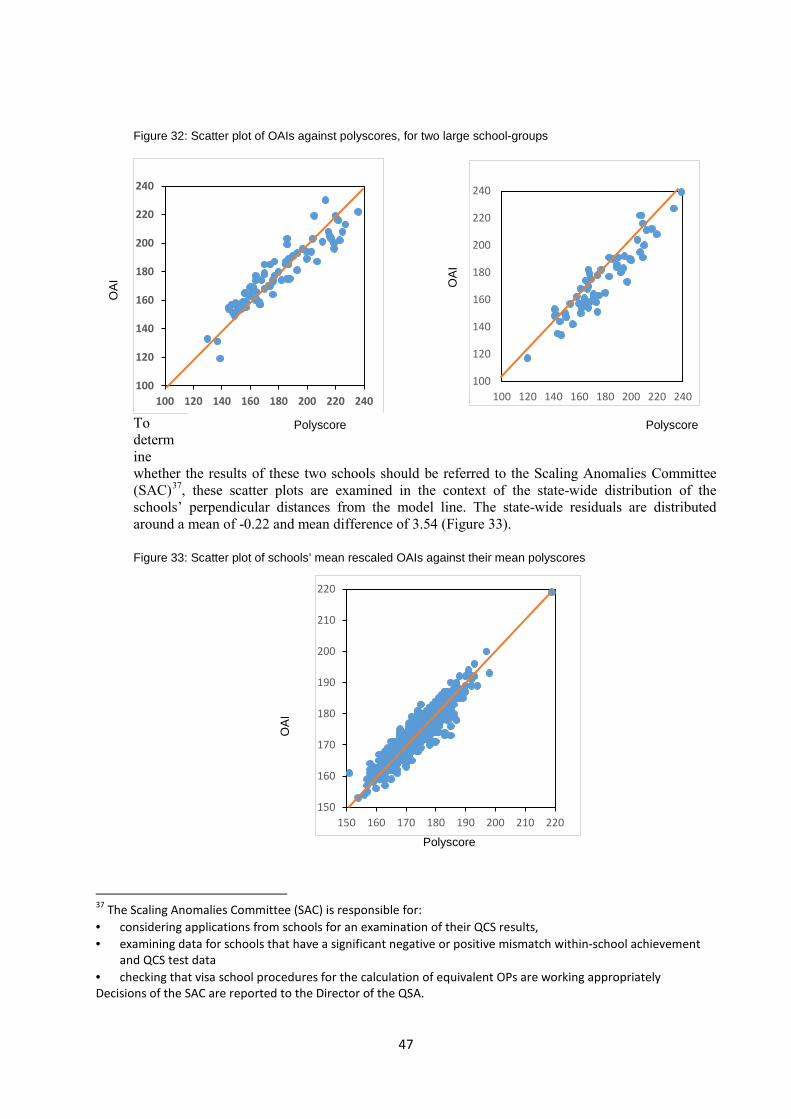
47

100

120

140

160

180

200

220

240

100 120 140 160 180 200 220 240

O

AI

150

160

170

180

190

200

210

220

150 160 170 180 190 200 210 220

100

120

140

160

180

200

220

240

100 120 140 160 180 200 220 240

Figure 32: Scatter plot of OAIs against polyscores, for two large school-groups

To determine whether the results of these two schools should be referred to the Scaling Anomalies Committee (SAC)37, these scatter plots are examined in the context of the state-wide distribution of the schools’ perpendicular distances from the model line. The state-wide residuals are distributed around a mean of -0.22 and mean difference of 3.54 (Figure 33).

Figure 33: Scatter plot of schools’ mean rescaled OAIs against their mean polyscores

Polyscore

37 The Scaling Anomalies Committee (SAC) is responsible for: · considering applications from schools for an examination of their QCS results, · examining data for schools that have a significant negative or positive mismatch within-school achievement

and QCS test data · checking that visa school procedures for the calculation of equivalent OPs are working appropriately Decisions of the SAC are reported to the Director of the QSA.

OA

I

Polyscore Polyscore

O

AI

48

The first school’s mean difference is close to the statewide mean while the second lies approximately 1.2 mean differences from the state mean. Neither mean could be regarded as an outlier. 47.6 QSA intervention plots School intervention plots, as shown below, are prepared to determine whether the results of individual schools should be referred to the Scaling Anomalies Committee (SAC). Because the likely cause of an excessive proportion of negative differences in a school-group is a mismatch in the scaling of the SAIs by the QCS test scores, the school intervention plots focus on differences between QCS test scores and polyscores. The mismatch can result in the mean QCS test score being substantially lower than it should be or the mean difference being substantially larger than it should be, so two intervention plots are required. Figure 3438 shows the QCS–polyscore difference plotted against the QCS mean and the Figure 35 shows the QCS–polyscore difference plotted against the QCS mean difference.

Each point represents a separate school. If the school is an outlier, lying below the 5th percentile it is referred to the SAC. If there is enough evidence to support a change, the SAC can

38 Guideline for determining Overall Positions (OPs) and Field Positions (FPs), page 24. Queensland Studies Authority.

Figure 34 QCS – Polyscore difference Figure 35 QCS – Polyscore mean difference plotted against QCS mean plotted against QCS mean difference

49

recommendation an intervention. Either the mean or mean difference can be modified to reduce the mismatch but cannot eliminate it entirely.

In the above figures the two crosses represent the position of a school with regard to the mean and mean difference. The school would not be regarded as an outlier as it above the 5th percentile in both figures.

50

8. CALCULATING OVERALL AND FIELD POSITIONS

8.1 Banding OAIs into OPs Following the calculation of the OAIs, the final step is to derive broader measures of achievement, the Overall Positions. There are 25 OPs, with 1 representing the highest level and 25 the lowest. In keeping with Queensland’s underlying philosophy there are no pre-determined percentages of OP-eligible students in the bands the band boundaries are determined so that the OP bands will give comparable standards from one year to the next. Following the procedures used in earlier stages of the OP calculations, redundancy is built into the banding of OAIs into OPs to increase the reliability of the final set of estimates. Two methods are used; one based on levels of achievement and the other based on the QCS test. Equating methods based on levels of achievement depend on the assumption that levels of achievement represent comparable standards from year to year. One procedure uses multiple regression to model OAI as a function of dummy variables that represent levels of achievement in Authority subjects for each year. A linear transformation that minimises the differences between pairs of regression coefficients is then applied to the OAI scales. In a second procedure students in one year are matched with students in the other year who have completed the same subjects and have similar patterns of grades in their courses and who have similar QCS test scores. A linear transformation that minimises the differences between the pairs of OAIs is then applied. In the second method QCS test scores from the two years are first equated using Item Response Theory (IRT) modelling using links developed through trial data. The linear relationship between OAI and QCS test scores is then used to match the distributions of OAI scores. The sets of estimates are combined to determine the band boundaries to be used for the current year. 8.2 Banding FAIs into FPs

In contrast to the OPs, which are meant to represent comparable standards from year to year, FPs are constructed to give a smooth distributions, unequal divisions and discrimination at the upper end. For each FP there are 10 bands, with 1 being the highest. For each field the state-wide distribution of the corresponding FAIs is first divided into five regions:

· upper (4% of the total) · intermediate above ( about 14-15% of the total) · middle (about 625 of the total) · intermediate below (about 9-10% of the total) · lower (6% of the total)

The intermediate region is divided into two bands so that there is a steady change in size from the upper to the highest of the middle bands. The middle region is divided into five bands set at the average of those cut-offs required to produce equal numbers of persons and equal bandwidths divisions of the FAI scale. 8.3 Individual student anomaly detection

51

The outcomes of the tertiary entrance calculations for individual students are also subject to scrutiny to ensure that application of the standard processes have not disadvantaged individuals. Each student’s OP is compared with those of students who studied a similar combination of subjects and achieved similar grades and also had similar QCS test scores. Specific cases, where students’ OPs are considered to be anomalously low in comparison their comparison groups, are considered by a QSA committee chaired by the Deputy Director of the Assessment and Reporting Division. Data presented to the committee include are a set of four plots, information about levels of achievement in subjects, comments from the moderation panel about the school’s application of assessment standards and QCS test performance. Two of the plots are shown below. The first is a plot of students’ OAI against the average of their best five grades, and the second is a plot of students’ OAI against their polyscores. Figure 3639: Plot of students’ OAIs against the average of their best five levels of achievement

Figure 37: Plot of students’ OAIs against their polyscores

In examining the plots and other evidence the committee decides whether or not the student’s OP constitutes an outlier with compared to other students. If the committee decides that the OP is an outlier it must then determine whether an adjustment is warranted and the extent of the adjustment. The plots show the position of the student in question and a position recommended by the Deputy Director of the Assessment and Reporting Division if the committee decides that the OP is an outlier. Typically the change will be one position on the OP scale. 39 Guideline for determining Overall Positions (OPs) and Field Positions (FPs), page 25. Queensland Studies Authority, November 2012

52

8.4 Discussion The anomaly detection procedures, at individual and school level, are typical of the care and attention to detail in the QSA procedures to ensure that students are treated fairly and receive the results they deserve. After the issue of the Tertiary Entrance Statement students may also apply for a review of their OP.

53

9. OVERALL AND FIELD POSITIONS IN 2013

9.1 Overall Positions in 2013 In 2013 15,883 students were eligible for OPs. Table 26 and Figure 38 show the distribution of OP-eligible students across the 25 bands. Since 2005 the percentage of OP-eligible students receiving an OP 1 has increased from 2% and the percentage receiving OP 25 has decreased, which can be seen as a consequence of a reduction in the proportion of Year 12 students who are OP-eligible during this period. It is assumed that that lower achieving students who would have received OPs in these lower bands are choosing pathways that do not result in OP-eligibility. The distribution of OPs is skewed, as demonstrated in the following table and frequency table. The percentage of OPs in the bands increase from 2.7% in band 1 to 6.2% in band 11. The percentages in the bands then decrease from band 13. There are very few students in the lower bands. Table 29: Distribution of OP-eligible students across OP bands40

OP band N % OP band N %

1 711 2.7 14 1,531 5.9

2 8885 3.4 15 11,473 5.7

3 11,109 4.3 16 11,293 5.0

4 1,205 4.7 17 11,178 4.5

5 1,256 4.8 18 9,903 3.5

6 11,376 5.3 19 7,776 3.0

7 11,476 5.7 20 5,572 2.2

8 11,572 6.1 21 3,350 1.3

9 11,576 6.1 22 1,180 0.7

10 11,588 6.1 23 94 0.7

11 11,610 6.2 24 36 0.1

12 1,561 6.0 25 3 0.0

13 1,561 6.0

40 2013 Data summary – state distribution of Overall Positions and Field Positions. Queensland studies Authority.

54

0

200

400

600

800

1000

1200

1400

1600

1800

1 2 3 4 5 6 7 8 9 10 11 12 13 14 15 16 17 18 19 20 21 22 23 24 25

Figure 38: Histogram of OPs for non-visa students, 2013

Bands

As is evident from the data presented in the following figure (Figure 39) there has been very little change in the distribution of OPs from 2012 to 2013. Figure 39: Relative frequency histograms of OPs for 2012 and 2013

9.2 Gender differences in Overall Positions

Females are over-represented in the OP-eligible cohort so, when comparing the performance of males and females, the relative achievements are compared.

0

1

2

3

4

5

6

7

1 2 3 4 5 6 7 8 9 10 11 12 13 14 15 16 17 18 19 20 21 22 23 24 25

r

Per

cent

age

2012 2013

Fr

eque

ncy

55

Table 30: Relative frequencies of OPs by gender41

OP band

Females Males OP band

Females Males

N % N % N % N %

1 341 2.4 370 3.3 14 820 5.6 711 6.3

2 503 3.5 382 3.4 15 754 5.2 719 6.3

3 652 4.5 457 4.0 16 675 4.6 618 5.4

4 706 4.9 499 4.4 17 638 4.4 540 4.8

5 758 5.2 498 4.4 18 462 3.2 441 3.9

6 872 6.0 504 4.4 19 388 2.7 388 3.4

7 919 6.3 557 4.9 20 276 2.0 296 2.6

8 939 6.5 633 5.6 21 173 1.2 177 1.6

9 938 6.4 638 5.6 22 84 0.6 96 0.8

10 948 6.5 640 5.6 23 47 0.3 47 0.4

11 900 6.2 710 6.3 24 18 0.1 18 0.2

12 861 5.9 708 6.2 25 3 0.0 0 0.0

Figure 40: Relative histograms of OPs by males and females

Female Male The data show clearly that while there are proportionally more males than females in OP 1, females are over-represented in the subsequent bands from OP 2 to OP 11. Males are then over-represented in the lower bands. This is in contrast to the distributions of grades in the QCS test, where males were over-represented in the higher grades and females over-represented in the lower bands. 9.3 Field Positions in 2013 Because Year 12 students are free to choose from a range of subjects, not all OP-eligible students are eligible for all Field Positions. Table 31 shows the number and percentage of OP-eligible students who were eligible for each FP. Almost all were eligible for Field A and most were

41 2013 Data summary State distribution of Overall Positions and Field Positions, page 3.Queensland Studies Authority

Per

cent

age

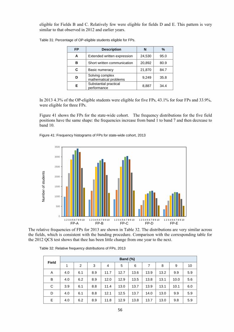
56

0

500

1000

1500

2000

2500

3000

3500

1 2 3 4 5 6 7 8 9 10 1 2 3 4 5 6 7 8 9 10 1 2 3 4 5 6 7 8 9 10 1 2 3 4 5 6 7 8 9 10 1 2 3 4 5 6 7 8 9 10 FP-A FP-B FP-C FP-D FP-E

eligible for Fields B and C. Relatively few were eligible for fields D and E. This pattern is very similar to that observed in 2012 and earlier years. Table 31: Percentage of OP-eligible students eligible for FPs.

FP Description N %

A Extended written expression 24,530 95.0

B Short written communication 20,892 80.9

C Basic numeracy 21,870 84.7

D Solving complex mathematical problems 9,249 35.8

E Substantial practical performance 8,887 34.4

In 2013 4.3% of the OP-eligible students were eligible for five FPs, 43.1% for four FPs and 33.9%, were eligible for three FPs.

Figure 41 shows the FPs for the state-wide cohort. The frequency distributions for the five field positions have the same shape: the frequencies increase from band 1 to band 7 and then decrease to band 10. Figure 41: Frequency histograms of FPs for state-wide cohort, 2013

The relative frequencies of FPs for 2013 are shown in Table 32. The distributions are very similar across the fields, which is consistent with the banding procedure. Comparison with the corresponding table for the 2012 QCS test shows that thee has been little change from one year to the next.

Table 32: Relative frequency distributions of FPs, 2013

Field Band (%)

1 2 3 4 5 6 7 8 9 10

A 4.0 6.1 8.9 11.7 12.7 13.6 13.9 13.2 9.9 5.9

B 4.0 6.2 8.9 12.0 12.9 13.5 13.8 13.1 10.0 5.6

C 3.9 6.1 8.8 11.4 13.0 13.7 13.9 13.1 10.1 6.0

D 4.0 6.1 8.8 12.1 12.5 13.7 14.0 13.0 9.9 5.9

E 4.0 6.2 8.9 11.8 12.9 13.8 13.7 13.0 9.8 5.9

Num

ber o

f stu

dent

s

57

FP-A FP-B FP-C FP-D FP-E

02000400060008000

10000120001400016000

F M F M F M F M F M

9.4 Gender differences for Field Positions Figure 42 shows the number of males and females in each of the five field positions. In 2013 females were over-represented in fields A, B and E, and males over-represented in fields C and D. Figure 42: Frequency distribution of males and females by Field Position

Table 3342 shows the distributions of FPs for males and females. Proportionally more females than males are in the higher bands for all fields except Field D which is solving complex problems involving mathematical symbols and abstractions.

Table 33: Frequency distributions of students’ FPs within gender

Band (%)

1 2 3 4 5 6 7 8 9 10

A

All 4.0 6.2 8.9 11.7 12.7 13.6 13.9 13.2 9.9 5.9

Female 4.7 7.1 10.3 13.3 13.8 14.0 13.1 11.8 8.0 4.0

Male 3.2 4.9 6.9 9.5 11.3 13.0 15.0 15.2 12.6 8.4

B

All 4.0 6.2 8.9 12 12.9 13.5 13.8 13.1 10.0 5.7

Female 4.3 6.9 9.7 13.3 13.9 14 13.1 11.7 8.5 4.6

Male 3.6 5.2 7.7 10 11.5 12.9 14.8 15.0 12.1 7.2

C

All 3.9 6.1 8.8 11.4 13.0 13.7 13.9 13.1 10.1 6.0

Female 3.1 5.8 8.9 12.3 13.7 14.2 13.6 12.5 10.0 5.9

Male 4.9 6.4 8.7 10.4 12.1 13.2 14.2 13.8 10.2 6.1

D

All 4.0 6.1 8.8 12.1 12.5 13.7 14.0 13.0 9.9 6.0

Female 3.2 6.3 9.7 13.3 13.2 15.4 13.8 12.3 8.1 4.6

Male 4.5 6.0 8.2 11.3 12.1 12.6 14 13.4 11.0 6.8

E

All 4.0 6.2 8.9 11.8 12.9 13.8 13.7 13.0 9.9 5.9

Female 4.5 7.3 10.1 13.7 13.8 12.8 12.7 11.9 8.6 4.6

Male 3.2 4.5 6.9 8.8 11.5 15.4 15.2 14.7 11.8 8.2

42 2013 Data summary State distribution of Overall Positions and Field Positions, page 6. Queensland Studies Authority

Fr

eque

ncy

58

9.5 Discussion Overall, the results for the Overall Positions and Field Positions are little changed from those of previous years.

59

BIBLIOGRAPHY

A. Queensland Studies Authority publications downloaded from www.qsa.qld.edu.au

(i) Statistical reports 2013 Data summary: Year 12 enrolment and certification 2013 Data summary: QCS attendance and grades. 2013 Data summary State distribution of Overall Positions and Field Positions Subject enrolments and levels of achievement - 2013 (ii) Queensland Certificate of Education Information for Qld 2010 Year students who will not be eligible of and OP (updated with 2010 data) Queensland Certificate of Education Review of aspects of the Queensland Certificate of Education (2011) School-based assessment, the Queensland system Senior Education Profile Senior education profile reports: Preparation, distribution, appeals- 2007 Tertiary Entry Procedures in Queensland Tertiary entrance review procedures (iii) Student Achievement Indicators (SAIs) BonSAI User guide Random sampling project. 2013 Report on random sampling of assessment in Authority subjects Form R6 Subject Achievement Indicators (SAIs) Fact Sheet 1: The basics Subject Achievement Indicators (SAIs) Fact Sheet 2: BonSAI Subject Achievement Indicators (SAIs) Fact Sheet 3: How QSA checks SAIs Subject Achievement Indicators (SAIs) Fact Sheet 4: What to do if QSA calls about SAIs Subject Achievement Indicators (SAIs) Fact Sheet 5: Checking SAI ratio multiplicity be – what should it be? (iv) Queensland Core Skills Test Common Curriculum Elements (CCEs) Fielding, December 2008 QCS Test Guideline (2013) QCS Retrospective 2013 Queensland Core Skills Test 2011 Yearbook Queensland Core Skills Test 2012 Yearbook Queensland Core Skills Test 2013 Yearbook Retrospective Core Skills Test 2012 Retrospective Core Skills Test 2013 Student Information Bulletin. All you need to know about the Queensland Core Skills Test, 2013 (v) Calculating Overall Positions and Field Positions Calculating OPs: The basic principles, 2012 Eligibility for Overall Positions (OPs) Eligibility for Field Positions (FPs)

60

Fast Facts Field Positions (FPs) Subject weights for 2013 Guideline for determining Overall Positions (OPs) and Field Positions (FPs) – November 2012 Procedures for calculating Overall Positions (OPs) and Field Positions (FPs) December 2011 Technical features of the OP/FP system – 2010 Visa student procedures: Equivalent Overall Positions (OPs) and Field Positions (FPs) 2008 B. Other publications Allen, R. (2013) Strengths and weaknesses of Queensland’s OP system today. Bennett, J., Cooney, G., Edwards. B. and Tognolini, J. (2012) A Review of the Queensland Core Skills (QCS) Test to ascertain the ongoing relevance of the test and the capability of the test to act as a statistical scaling device in the calculation of Overall Positions (OPs) and Field Positions (FPs). David, H. A. (1987) Ranking from unbalanced paired-comparison data. Biometrika, 74, 2, pp432-436. Kelly, D. (2014) An analysis of earlier reports into Senior assessment and tertiary entrance procedures in Queensland. Marion, S.F., Peck, P. and Raymond, J (2011) Year-to-year comparability of results in Queensland Studies Authority Senior Secondary courses that include school-based assessments: an ACACA sponsored review. Pitman, J.A. 1987. Tertiary Entrance in Queensland: A Review Radford, W. (1970) Public Examinations for Queensland Secondary Schools. Queensland Department of Education, Brisbane. Scott, E. (Chairman), 1878. A review of school-based assessment on Queensland secondary schools. Board of Secondary School Studies. Brisbane.

Sympson, J.B. & Haladyna, T.M. (1988) An evaluation of “polyweighting” in domain-referenced testing. Paper presented at the Annual Meeting of the American Educational Research Association. New Orleans, LA, April 5-9, 1988.

Viviani, N. (1990) Review of Tertiary Entrance in Queensland. Report submitted to Minister for Education.