Review of ray-Born forward modeling for migration and diffraction analysis
TIJMEN JAN MOSER
van Alkemadelaan 550A, 2597 AV ’s-Gravenhage, The Netherlands ([email protected])
Received: August 20, 2011; Revised: October 20, 2011; Accepted: October 27, 2011
ABSTRACT
The ray-Born approximation is a very useful tool for forward modeling of scattered waves. The fact that ray-Born modeling underlies most seismic migration techniques, and therefore shares their assumptions, is a justification in itself to consider it for forward modeling. The ray-Born approximation does not make an explicit distinction between specular reflections and nonspecular diffractions. It therefore allows the modeling of diffractions from structural discontinuities such as edges and tips, as well as caustic diffractions. In the simplest implementation ray-Born seismograms are multiple-free. Ray-Born modeling can be orders of magnitude faster than finite-difference modeling, both in two-and three dimensions.
Ke y wo r d s : computational seismology, seismic migration, diffractions, wave propagation
1. INTRODUCTION
Most seismic migration techniques are based on inverse scattering theory (Tarantola, 1984; Beylkin and Burridge, 1990). They assume a smooth and known subsurface background, in which wave propagation can be accurately modeled, e.g., by asymptotic ray theory. Unknown scatterers or perturbations on the background, causing backscattering to the surface in the form of reflections and diffractions observed in the seismic data, are the objective of inversion by migration. Forward modeling of the seismic response of the scatterers is an essential component of migration. For backscattering this is usually done by the first-order term of the Born scattering series (Beydoun and Tarantola, 1988).
The forward modeling by ray-Born modeling is a very useful tool in itself which has been studied in many publications (Červený, 2001, and references listed there, see also Chapman, 2004). It is closely related to demigration, the process whereby synthetic seismic sections are generated from a migrated image (Santos et al., 2000). The fact that ray-Born modeling underlies most seismic migration techniques, and therefore shares their assumptions, is a justification in itself to consider it for forward modeling. Depending on its implementation and the definition of the background model, ray-Born modeling has the potential to model the first-order scattering in structural models of arbitrary complexity, i.e. there are no restrictions to so-called layer-cake models or
T.J. Moser
412 Stud. Geophys. Geod., 56 (2012)
raytracing-friendly models. If the scatterers are aligned along smooth horizons, the scattering response consists of specular reflections. Additionally, if the scatterers are not restricted to smooth horizons and the scattering is not restricted to specular reflection, ray-Born modeling has the potential to model diffractions from discontinuities and small scattering objects.
There are several key applications of ray-Born modeling. First, it can serve to generate synthetic data under controlled and idealized circumstances for the testing of migration algorithms - a useful property in this regard is that first-order scattering involves primaries only. Second, it can be used to study the effect of small modifications of an existing subsurface model (scenario testing). Third, for a given subsurface model it can be used to investigate illumination of a migration target and help in acquisition survey design.
This paper reviews some of the properties of ray-Born modeling and discusses some of its benefits, with special attention paid to diffractions from structural edges and small scattering objects.
2. BASIC DERIVATIONS
This section reviews some well-known material relevant to the following sections. For simplicity, it considers only acoustic wave propagation in a three-dimensional isotropic inhomogeneous velocity model.
2 . 1 . B o r n A p p r o x i m a t i o n
Consider the scalar wave equation in frequency domain in an isotropic inhomogeneous velocity model c(x)c(x):
where u(x; !)u(x; !) is a wave function dependent on the location xx and frequency !!, ¢¢ is the Laplace operator and s(x; !)s(x; !) is a source function. Scattering theory assumes that the velocity model can be decomposed into a slowly varying background model c0(x)c0(x) and a rapidly varying scatterer c1(x)c1(x):
c(x) = c0(x) + ²c1(x)c(x) = c0(x) + ²c1(x) , (2)
where ² > 0² > 0 is a dimensionless parameter. The background Green’s function g0g0 is defined by
for a point source at yy . The background wave u0u0, which is the solution to Eq.(1) for c1 ´ 0c1 ´ 0, is given in terms of the Green’s function by
u0(x; !) =
Zg0(x; y; !)s(y; !)dyu0(x; !) =
Zg0(x; y; !)s(y; !)dy . (4)
The integral over yy extends over the source region, where s(y; !) 6= 0s(y; !) 6= 0. A general solution
Ray-Born for migration and diffraction analysis
Stud. Geophys. Geod., 56 (2012) 413
to Eq.(1) is assumed in the form of a scattering series
u =
1Xk=0
uk²k = u0 + ²u1 + ²2u2 + O(²3) (²! 0)u =
1Xk=0
uk²k = u0 + ²u1 + ²2u2 + O(²3) (²! 0) , (5)
where u0u0 is the background wave, u1u1 the first-order scattered wave and ukuk (k > 1k > 1) higher-order scattering terms. Inserting Eqs.(5) and (2) in Eq.(1), using Eq.(4) and collecting linear terms in ²² leads to
u1(r; !) = !2
Zg0(r;x; !)V (x)u0(x; !)dxu1(r; !) = !2
Zg0(r;x; !)V (x)u0(x; !)dx , (6)
where rr is a receiver point. The expression
V (x) = 2c1(x)c¡30 (x)V (x) = 2c1(x)c¡30 (x) (7)
is referred to as the scattering potential and the integral over xx extends over the support of the scatterer, or the region where V (x) 6= 0V (x) 6= 0. Inserting Eq.(4) in Eq.(6) gives an expression for u1u1 in terms of the source function ss:
u1(r; !) = !2
Z Zg0(r;x;y; !)V (x)s(y; !)dxdyu1(r; !) = !2
Z Zg0(r;x;y; !)V (x)s(y; !)dxdy , (8)
where g0(r;x; y; !) = g0(r; x; !)g0(x; y; !)g0(r;x; y; !) = g0(r; x; !)g0(x; y; !). For a point source at ss , so that s(y; !) = s(!)±(y ¡ s)s(y; !) = s(!)±(y ¡ s), (8) reads:
u1(r; s; !) = !2s(!)
Zg0(r;x; s; !)V (x)dxu1(r; s; !) = !2s(!)
Zg0(r;x; s; !)V (x)dx . (9)
Expressions (6), (8) and (9) are the (first-order) Born approximation for the scattered field in terms of the general Green’s function g0g0 defined by Eq.(3). It relates a velocity perturbation linearly to the observed scattered wave field, and therefore plays a central role in imaging and migration. The next section discusses Green’s functions based on asymptotic ray theory.
2 . 2 . R a y - B o r n A p p r o x i m a t i o n
In asymptotic ray theory the high-frequency approximation to the background elementary Green’s function (3) has the form
where T (x; y)T (x; y) and A(x; y)A(x; y) are the ray-based travel-time and amplitude at a point xx for a point source at yy . Expressions for T (x; y)T (x; y) and A(x; y)A(x; y) are found by substituting Eq.(10) in Eq.(3) and collecting terms with equal power in !!. The two highest order terms in !! give the eikonal and transport equations
where the gradient rr and Laplacian ¢¢ are taken with respect to xx. Rays are the characteristic curves of the eikonal equation given by kinematic ray equations:
for arclength ss and slowness vector pp. The travel time along a ray from yy to xx is found by integrating the inverse velocity c0c0 along it
T =
Z s1
s0
c¡10 (x(s))dsT =
Z s1
s0
c¡10 (x(s))ds . (14)
where x(s0) = yx(s0) = y and x(s1) = xx(s1) = x. At any point along the ray, kinematic ray tracing gives rT = prT = p and dynamic ray tracing allows to compute ¢T¢T . The amplitude A(x; y)A(x; y) follows then from integrating the transport equation (12) along the ray. In case of multipathing, the expression (10) is replaced by
where the index nn runs over all rays between xx and yy , TnTn is the travel time along the ray nn and AnAn its amplitude. The KMAH index kn(x; y)kn(x; y) counts the number of caustics along ray nn and accounts for the corresponding phase shift. At caustics the amplitude is singular. See Červený (2001) for details on kinematic and dynamic ray tracing and many references.
A simple form for the frequency domain ray-Born approximation for acoustic wave scattering follows from inserting Eq.(10) in Eq.(9):
where A(r;x; s) = A(r; x)A(x; s)A(r;x; s) = A(r; x)A(x; s) and T (r;x; s) = T (r; x) + T (x; s)T (r;x; s) = T (r; x) + T (x; s). The time domain version of Eq.(16) is:
U(r; s; t) =
ZA(r;x; s)V (x)S00(t¡ T (r;x; s))dxU(r; s; t) =
ZA(r;x; s)V (x)S00(t¡ T (r;x; s))dx , (17)
where tt is the recording time and S 00(t)S 00(t) the second-order time derivative of the source wavelet. Expression (17) is the starting point for subsequent discussions in this paper.
3. VALIDITY
The Born approximation (6 9) has a clear physical interpretation in terms of scattering. The first-order scattered wave u1u1 consists of two parts: a background wave propagating from the source through the background medium c0c0 to the point xx, where it interacts with the scatterer c1(x)c1(x), and then propagates from xx through the background
Ray-Born for migration and diffraction analysis
Stud. Geophys. Geod., 56 (2012) 415
medium to the receiver rr. Non-linear scattering is accounted for by higher order terms uk (k > 1)uk (k > 1) in the scattering series (5) and includes multiple reflections (Weglein et al., 2003). Expressions for ukuk follow by recursively applying Eq.(6) for k > 1k > 1:
uk(r; !) = !2
Zg0(r;x; !)V (x)uk¡1(x; !)dxuk(r; !) = !2
Zg0(r;x; !)V (x)uk¡1(x; !)dx . (18)
The series (5) is convergent if ² < 1² < 1 and the terms ukuk are globally bounded, subject to a suitable norm jj:jjjj:jj and independently of kk . These conditions are satisfied if
jj !2
Zg0(r;x; !)V (x)dxjj · 1jj !2
Zg0(r;x; !)V (x)dxjj · 1 , (19)
so that each term in the scattering series is small compared to its previous term. The (first-order) Born approximation becomes practical if higher order terms can be ignored (that is, when ·· is replaced by ¿¿ in Eq.(19)). For this reason, the Born approximation is called a weak-scattering approximation (Keller, 1969; Natterer, 2004).
Equation (17) for the ray-Born approximation is a simple and pragmatic formula to apply, which can be made as general and rigorous as needed. It is approximate for finite frequencies and a finite scattering potential, but becomes exact, in asymptotic sense, in the high-frequency limit ! ! 1! ! 1 and weak-scattering limit j R V (x)dxj ! 0j R V (x)dxj ! 0. Therefore, in asymptotic sense, the ray-Born integral results in correct kinematics, for specular reflections as well as (non-specular) diffractions. For correct amplitudes AA and in asymptotic sense, the dynamics are correct as well. For the acoustic case and constant density, the scattering potential has the meaning of the perturbation of the quadratic slowness: V (x) » ±(c¡2(x))V (x) » ±(c¡2(x)) (where cc is the P-velocity). Equation (17) can be readily generalized to elastic (Beydoun and Mendes, 1989; Beylkin and Burridge, 1990) and anisotropic (Červený, 2001, Section 2.6.2) cases.
An important observation is that the ray-Born approximation only requires that the integral (17) exists and is bounded, but does not pose any further restriction on the smoothness of the scatterer c1(x)c1(x). In particular, there is no distinction between reflections and diffractions. This property is further elaborated on in Section 6 on Diffractions. Another consequence is that the ray-Born approximation remains valid for scattering geometries of considerable complexity. This is further developed in Section 4 on Implementation and Section 5 on Properties.
The weak-scattering approximation is sometimes seen as a limitation in presence of a strong model contrasts, and particularly to the use of the Born approximation in seismic migration. However, it must be noted that every migration technique based on a model decomposition in a smooth background and rapidly varying perturbation (as Eq.(2)) requires an accurate background model to obtain a kinematically accurate image, and therefore a small perturbation c1c1. The challenge of forward modeling in migration is not posed by strong scattering contrast at interfaces separating smooth layers, but by accurate kinematics within the layers. An accurate background model therefore implies weak-scattering and validates the Born approximation.
An alternative validity criterion of the Born approximation is a low-frequency approximation; however, since this conflicts with common high-frequency approximations in the Green’s functions (in particular the approximation based on ray
T.J. Moser
416 Stud. Geophys. Geod., 56 (2012)
theory) as well as in the imaging formulae (in particular the diagonal approximation of the Hessian (Tarantola, 1984), the weak-scattering formulation is to be preferred. Either way, the ultimate validity criterion for the ray-Born approximation is Eq.(19).
It follows from Eqs.(6), (8), (9) and (18) that the background Green’s function g0(x; y; !)g0(x; y; !) plays an important role in forward modeling (even for higher order scattering) and hence in inversion/migration (Nita et al., 2004). On the other hand, the full wave’s Green’s function, g(x; y; !)g(x; y; !), which is the solution to Eq.(1) for s(x; !) = ±(x ¡ y)s(x; !) = ±(x ¡ y), hardly plays any role in practical algorithms; first because it depends on the scatterer c1(x)c1(x), which is unknown and the objective of imaging algorithms, and second, because the scatterer itself does not meet the smoothness requirements of several techniques for forward modeling. For this reason, the notion of the perturbation of the Green’s function (e.g. ±g = g ¡ g0±g = g ¡ g0) appearing in some publications can be misleading.
4. IMPLEMENTATIONS
Ray-Born forward modeling (17) consists of two components: the computation of the Green’s functions and the evaluation of the scattering integral. The computation of the Green’s functions based on ray theory assumes that the background model is suitable for ray tracing. Such a background can be characterized as raytracing-friendly.
A particular example of ray-Born modeling using a raytracing-friendly model is presented by Červený and Coppoli (1992). Here, the background consists of laterally varying layers with smooth interfaces; the Green’s functions are computed by kinematic ray tracing for the travel times and dynamic ray tracing for the geometrical spreading, taking into account the necessary interface transforms. The amplitudes are computed using the geometrical spreading and the accumulated product of reflection/transmission coefficients at the interfaces. Červený and Coppoli (1992) use this design for the modeling of diffractions from isolated scattering objects.
A common raytracing-friendly background, considered in this paper, is a fully smooth background in which the scatterers account for any type of discontinuity (reflector or diffractor). The scattering then mimics wave propagation as assumed in many migration algorithms. The travel time can be computed by wavefront construction (Vinje et al., 1993; Lambaré et al., 1996), eikonal equation solvers (Sethian, 1996) or shortest path techniques (Moser, 1991; see Červený, 2001, Section 3.8, for further references). The preferred option depends on the background smoothness and the occurrence of multi-valued travel time fields. The amplitude can be computed by dynamic ray tracing if true-amplitude signals are the objective (Červený, 2001) or approximated if mainly kinematical properties are studied (Dellinger et al., 2000). However, a strong multivaluedness of the ray field in the background model poses difficulties for the ray-tracing component of ray-Born modeling. In such a case, either more advanced asymptotic modeling techniques such as Gaussian beams should be used, the background should be subdivided by introducing more scattering elements, or the background should be smoothed.
The second component of ray-Born modeling is the evaluation of the scattering integral (17). In general this is a volume integral over the support of VV (region where V (x) 6= 0V (x) 6= 0). Usually, it must be carried out numerically by decomposing VV into a collection of point scatterers. If the point scatterers are distributed over a volume,
Ray-Born for migration and diffraction analysis
Stud. Geophys. Geod., 56 (2012) 417
a volume integral is necessary. If the point scatterers are confined to horizons, the integral reduces to a surface integral which is very similar to the Kirchhoff modeling integral (Santos et al., 2000). If the point scatterers are isolated the integral can be replaced by a simple summation.
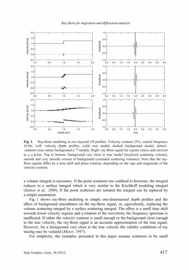
Fig. 1 shows ray-Born modeling in simple one-dimensional depth profiles and the effect of background smoothness on the ray-Born signal, or, equivalently, replacing the volume scattering integral by a surface scattering integral. The effect is a small time shift towards lower velocity regions and a rotation of the waveform; the frequency spectrum is unaffected. If either the velocity contrast is small enough or the background close enough to the true velocity, the ray-Born signal is an accurate approximation of the true signal. However, for a background very close to the true velocity the validity conditions of ray tracing may be violated (Moser, 1997).
For simplicity, the examples presented in this paper assume scatterers to be small
Fig. 1. Ray-Born modeling in two-layered 1D profiles. Velocity contrast 25%, central frequency 10 Hz. Left: velocity depth profiles, solid - true model; dashed - background model; dotted - scatterer (true minus background c¡2c¡2-model). Right: ray-Born signal for a point source and receiver at z = 0z = 0 km. Top to bottom: background very close to true model (localized scattering volume), smooth and very smooth version of background (extended scattering volumes). Note that the ray-Born signals differ by a time shift and phase rotation, depending on the sign and magnitude of the velocity contrast.
enough and confined to lines (in two dimensions) and surfaces (in three dimensions), so that volume integrals can be replaced by surface and line integrals. For completeness it is noted that surface and line integrals are to be evaluated with a proper measure relative to their parametrization (see textbooks on integration, e.g. Rudin, 1996).
5. PROPERTIES
As soon as the travel times and amplitudes are available for the Green’s functions in the background model, e.g. in the form of tables, the Born integral (17) is relatively easy to implement, in two- as well as three dimensions. Depending on the extent of the scattering potential, it can be evaluated efficiently, in most cases faster by orders of magnitude than finite-difference modeling. It does not rely on a grid for the propagation of waves, and therefore does not suffer from finite-difference artifacts such as grid diffractions and grid anisotropy. Moreover, there is no dispersion of the source signal (apart from the second time derivative at scattering) and there is full control over the amplitude spectrum of the generated data and their wavelet characteristics. In comparison to finite-difference modeling, there is no problem with instability of the modeling process. Sources and receivers can be located at arbitrary positions. Therefore a general acquisition geometry and surface topography can be considered. This contrasts with certain other forward modeling techniques that require sources and receivers to be confined to a regular grid or to plane surfaces.
Depending on the implementation and definition of the background, ray-Born modeling does not impose smoothness restrictions on the scattering geometry (such as ray-tracing modeling) and there are no dip limitations (such as with one-way wave equation modeling). The scatterers can be positioned at arbitrary locations in the model, so there are no restrictions to model topology (such as with layer-cake models). Also there are no over-rigorous consistency constraints, imposed by a model building logic. The ability to handle any model topology is a particular attractive property of ray-Born modeling, since it allows a considerable reduction in the time spent on laborious model building.
Ray-Born modeling solves the notoriously difficult two-point ray tracing problem on the fly, by automatically generating the scattering response at each receiver point for a given source point. The ray component of ray-Born (travel times and amplitudes, see Eq.(15)) is responsible for multipathing due to variations in the background model, the Born scattering naturally accounts for multipathing due to variations in reflector geometry (see Fig. 4a later). The physical nature of modeled data can be easily identified and scattered data events can be labeled with respect to propagation history.
Ray-Born modeling based on first-order scattering allows the study of primaries only. In many cases, this is an advantage; for instance, when generating synthetic data for the testing of migration algorithm, it can be useful to have them multiple-free. Multiple scattering (reflection/diffraction) can be included by repeated application of the Born integral (18), but this requires travel times and amplitudes from any point in the model to any other point and becomes computationally more expensive with an increasing multiple order.
Ray-Born for migration and diffraction analysis
Stud. Geophys. Geod., 56 (2012) 419
6. DIFFRACTIONS
Since Born scattering theory does not make assumptions with respect to scatterer geometry other than integrability, the forward modeling includes specular reflections from smooth horizons, as well as diffractions from discontinuities (edges, tips) and small scattering objects. If the integration is carried out accurately enough, reflections and diffractions are modeled with the same reliability. Therefore, various types of diffractions can be studied to a certain degree of accuracy using Born scattering. These include edge and tip diffractions (Klem-Musatov, 1994) and diffractions into the caustic shadow (Kravtsov and Orlov, 1993). One of the objectives of this paper is to demonstrate on simple examples that the properties of diffractions, in particular edge and tip diffractions, are correctly reproduced by the ray-Born approximation and to demonstrate its application to diffraction imaging.
On a terminological note, diffractions are to be distinguished from scattering: diffractions are the response to model discontinuities not modeled by standard ray theory, whereas scattering is the response to a perturbation on a background model. These are different mathematical descriptions which may, or may not, refer to the same physical phenomenon. For instance, reflections can be described by scattering but are different from diffractions. The term specularity refers to the validity of Snell’s law for reflection. It is recalled that Snell’s law consists of two statements: the incident and reflected slowness vectors are coplanar with the reflector normal and their components tangent to the reflector are equal. Edge and tip diffractions are scattered waves from (parts of) scattering objects which are non-differentiable and hence for which a normal cannot be defined.
The importance of diffraction analysis, modeling and imaging for seismic interpretation has been emphasized in many recent publications (see for instance Khaidukov et al., 2004; Moser and Howard, 2008; Pelissier et al., 2011). Conventional seismic processing and imaging uses specular reflections exclusively and disregards diffractions. On the other hand, diffractions carry valuable information concerning small, but significant, subsurface structural details that are lost in the conventional processing/imaging sequence. Diffractions permit high-resolution, or even super-resolution, imaging under favorable circumstances. Moreover, diffractions offer a different view on illumination of the imaging target. In particular, where steeply dipping reflectors are poorly visible on a standard surface seismic survey, diffractions are scattered in all directions and therefore observable irrespective of the acquisition aperture (Moser, 2009). The imaging of diffractions can be accomplished in several ways and is closely connected to focusing and velocity estimation (Reshef and Landa, 2009). Diffraction imaging algorithms which make use of an accurate velocity model have been discussed by Moser and Howard (2008).
Edge and tip diffractions have been introduced by Keller (1962) and studied in a number of papers leading up to the book by Klem-Musatov et al. (2008), where many references can be found. They have several properties based on the fact that they are corrections to reflected waves predicted by standard ray theory, which cast shadow zones at the edges and tips of a smooth reflector. First, at the shadow boundary the diffracted waveform is identical to the reflected waveform but has half its amplitude; second, the diffracted wave has a polarity reversal across the shadow boundary (Trorey, 1970). At
T.J. Moser
420 Stud. Geophys. Geod., 56 (2012)
tips, or the end points of a diffracting edge, tip diffractions are generated which have the same corrective properties to edge diffractions. The superposition of reflections, edge and tip diffractions is a smooth wave field, and the edge and tip diffraction coefficients are therefore called smearing factors, see Klem-Musatov et al. (2008) for details.
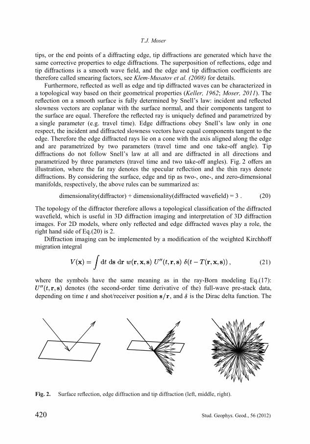
Furthermore, reflected as well as edge and tip diffracted waves can be characterized in a topological way based on their geometrical properties (Keller, 1962; Moser, 2011). The reflection on a smooth surface is fully determined by Snell’s law: incident and reflected slowness vectors are coplanar with the surface normal, and their components tangent to the surface are equal. Therefore the reflected ray is uniquely defined and parametrized by a single parameter (e.g. travel time). Edge diffractions obey Snell’s law only in one respect, the incident and diffracted slowness vectors have equal components tangent to the edge. Therefore the edge diffracted rays lie on a cone with the axis aligned along the edge and are parametrized by two parameters (travel time and one take-off angle). Tip diffractions do not follow Snell’s law at all and are diffracted in all directions and parametrized by three parameters (travel time and two take-off angles). Fig. 2 offers an illustration, where the fat ray denotes the specular reflection and the thin rays denote diffractions. By considering the surface, edge and tip as two-, one-, and zero-dimensional manifolds, respectively, the above rules can be summarized as:
The topology of the diffractor therefore allows a topological classification of the diffracted wavefield, which is useful in 3D diffraction imaging and interpretation of 3D diffraction images. For 2D models, where only reflected and edge diffracted waves play a role, the right hand side of Eq.(20) is 2.
Diffraction imaging can be implemented by a modification of the weighted Kirchhoff migration integral
V (x) =
Zdt ds dr w(r;x; s) U 00(t; r; s) ±(t¡ T (r;x; s))V (x) =
Zdt ds dr w(r;x; s) U 00(t; r; s) ±(t¡ T (r;x; s)) , (21)
where the symbols have the same meaning as in the ray-Born modeling Eq.(17): U 00(t; r; s)U 00(t; r; s) denotes (the second-order time derivative of the) full-wave pre-stack data, depending on time tt and shot/receiver position s/rs/r , and ±± is the Dirac delta function. The
Fig. 2. Surface reflection, edge diffraction and tip diffraction (left, middle, right).
Ray-Born for migration and diffraction analysis
Stud. Geophys. Geod., 56 (2012) 421
term ’full-wave’ is here to be understood as referring to the complete observed wave field, without separation into reflective and diffractive components. The migrated image is given by V (x)V (x), depending on the subsurface image point xx; it is compensated for geometrical spreading by a factor depending on xx which is not specified here. T (r; x; s)T (r; x; s) is the travel time from ss to rr via xx computed by ray tracing in a given reference velocity model. The extra weighting function w(r; x; s)w(r; x; s) (0 · w · 1)(0 · w · 1) is essential to design the Kirchhoff migration integral (21) for specific purposes. For w(r; x; s)w(r; x; s) identical to one we have the classical unweighted diffraction stack. Defining specularity SS by the scalar vector product
S (r; x; s) = nT Tx=jjTx jjS (r; x; s) = nT Tx=jjTx jj , (22)
and w = jSjw = jSj leads to stationary phase migration and w = 1 ¡ jS jw = 1 ¡ jS j to diffraction imaging (for details and references see Moser and Howard, 2008). In Eq.(22), TxTx denotes the gradient of T (r; x; s)T (r; x; s) with respect to xx. nn denotes the reflector unit normal, which depends on the image point xx.
A typical procedure for diffraction imaging consists of full-wave pre-stack depth migration (Eq.(21) with w ´ 1w ´ 1) with an adequate velocity model to obtain an optimally focused full-wave image V (x)V (x). From this image the reflector unit normal n(x)n(x) is obtained at each image point xx (Moser, 2010a). The diffraction image V D(x)V D(x) is then obtained by migrating using formula (21) with w = 1 ¡ jS jw = 1 ¡ jS j and SS given by Eq.(22).
The effect of specularity suppression (w = 1 ¡ jSj)(w = 1 ¡ jSj) in three-dimensional diffraction imaging of ray-Born modeled data is shown in the following section.
7. EXAMPLES
This section presents some examples of ray-Born modeling in two and three dimensions, meant to illustrate the statements made in the previous sections.
In all examples, the scatterers are assumed to be confined to lines or surfaces, and weak enough so that the scattering line integral and surface integral, respectively, provide an accurate Born signal (see Fig. 1 and discussion at the end of Section 4). The smooth background velocity models (in the examples of Figs. 4b, 5b and 6b later) have been chosen arbitrarily and loosely representative for the reflector geometry. Ray tracing in the smooth backgrounds was used to produce ray-based Green’s functions in these examples; for the other examples analytic expressions have been applied. For the two dimensional examples, the source signal has a central frequency of 7 Hz and the acquisition consists of 451 coincident source-receiver pairs along the surface z = 0z = 0 km; for the three dimensional examples relevant details are specified below.
The first example concerns a very simple horizontal line scatterer (Fig. 3a) at depth 3 km in a constant background medium with velocity 3 km/s. Two versions of the line scatterer are presented: one with a constant scattering potential (Fig. 3b solid line) and one with a scattering potential which is tapered towards the right edge point (Fig. 3b dashed line). The ray-Born integral (17) has been evaluated for these two scatterers. The zero-offset section over the constant line scatterer in Fig. 3c illustrates the capability of ray-Born modeling to generate reflected as well as diffracted wave field components. The two
T.J. Moser
422 Stud. Geophys. Geod., 56 (2012)
Fig. 3. a) Line scatterer model. b) Line scattering strength. Solid (straight) line: constant strength, section shown in Fig. 3c; dashed (curved) line: strength tapered to right, section shown in Fig. 3e. c) Line scatterer section. d) Amplitude spectrum line scatterer section (left/right: unbalanced/trace balanced). Note unchanged spectrum across shadow boundaries (at 5 and 10 km distance). e) Line scatterer section with taper. Note that the right edge diffraction has disappeared.
Ray-Born for migration and diffraction analysis
Stud. Geophys. Geod., 56 (2012) 423
edges of the line scatterer produce edge diffractions, which act as correction factors to the reflected wave. They have the smoothing property predicted by edge diffraction theory (Trorey, 1970; Klem-Musatov et al., 2008) - without them, the reflected wave component would be discontinuous, which is physically impossible. In particular, the properties of edge diffractions discussed by Trorey (1970) are distinguishable: the edge diffraction has a polarity reversal across the shadow boundary (or reflection tangent point, see arrows), its amplitude is half that of the reflection and the diffracted and reflected waveforms are equal (see amplitude spectra in Fig. 3d).
The section over the line scatterer with tapered scattering strength (Fig. 3e) further illustrates this smoothing property. At the right edge (at x = 10x = 10 km) the reflectivity is tapered to zero by a polynomial function of the distance xx. As a result the reflection terminates smoothly there without discontinuity, and no edge diffraction appears to correct for discontinuity - there is no need for a correction. Notably, this phenomenon depends on the degree of tapering and vanishing of higher order derivatives: to suppress the edge diffraction effectively, a taper of higher order than cubic is needed. Nevertheless, a slight residual curvature at the end of the reflected event is still visible. In all examples, a higher-order polynomial taper has been applied at model boundaries in order to suppress unwanted model boundary diffractions.
The next example is a syncline model (see Figs. 4ac), in which a triplication of the ray field occurs. The zero-offset section displayed in Fig. 4c shows the first-order Born response, computed by Eq.(17) and in a smooth background model; here, regular amplitude behaviour at the caustics can be observed, as well as caustic diffractions. Standard ray theory would result in a singularity at both caustics, with an infinite amplitude at the caustic and no signal beyond it. Arrows in Fig. 4c point to the caustic diffraction, which has, again, a smoothing effect on the wave field.
Fig. 4 Syncline model. a) Scatterer model; b) velocity model; c) syncline section - note caustic diffractions.
0123456
0 2 4 6 8 10 12 14
a)
Distance [km]
Dep
th [k
m]
0
0 5 10 15
5
b)
Distance [km]
Dep
thkm [
]
km/s
3
4
0
0 5 10 15
5
c)
Distance [km]
Tim
e [s
]
T.J. Moser
424 Stud. Geophys. Geod., 56 (2012)
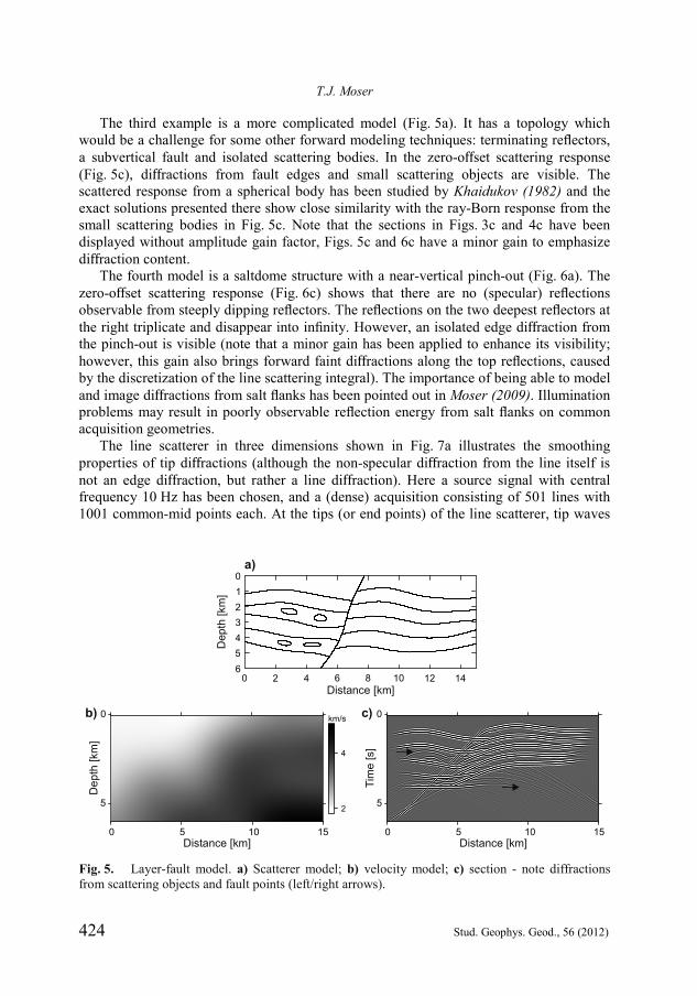
The third example is a more complicated model (Fig. 5a). It has a topology which would be a challenge for some other forward modeling techniques: terminating reflectors, a subvertical fault and isolated scattering bodies. In the zero-offset scattering response (Fig. 5c), diffractions from fault edges and small scattering objects are visible. The scattered response from a spherical body has been studied by Khaidukov (1982) and the exact solutions presented there show close similarity with the ray-Born response from the small scattering bodies in Fig. 5c. Note that the sections in Figs. 3c and 4c have been displayed without amplitude gain factor, Figs. 5c and 6c have a minor gain to emphasize diffraction content.
The fourth model is a saltdome structure with a near-vertical pinch-out (Fig. 6a). The zero-offset scattering response (Fig. 6c) shows that there are no (specular) reflections observable from steeply dipping reflectors. The reflections on the two deepest reflectors at the right triplicate and disappear into infinity. However, an isolated edge diffraction from the pinch-out is visible (note that a minor gain has been applied to enhance its visibility; however, this gain also brings forward faint diffractions along the top reflections, caused by the discretization of the line scattering integral). The importance of being able to model and image diffractions from salt flanks has been pointed out in Moser (2009). Illumination problems may result in poorly observable reflection energy from salt flanks on common acquisition geometries.
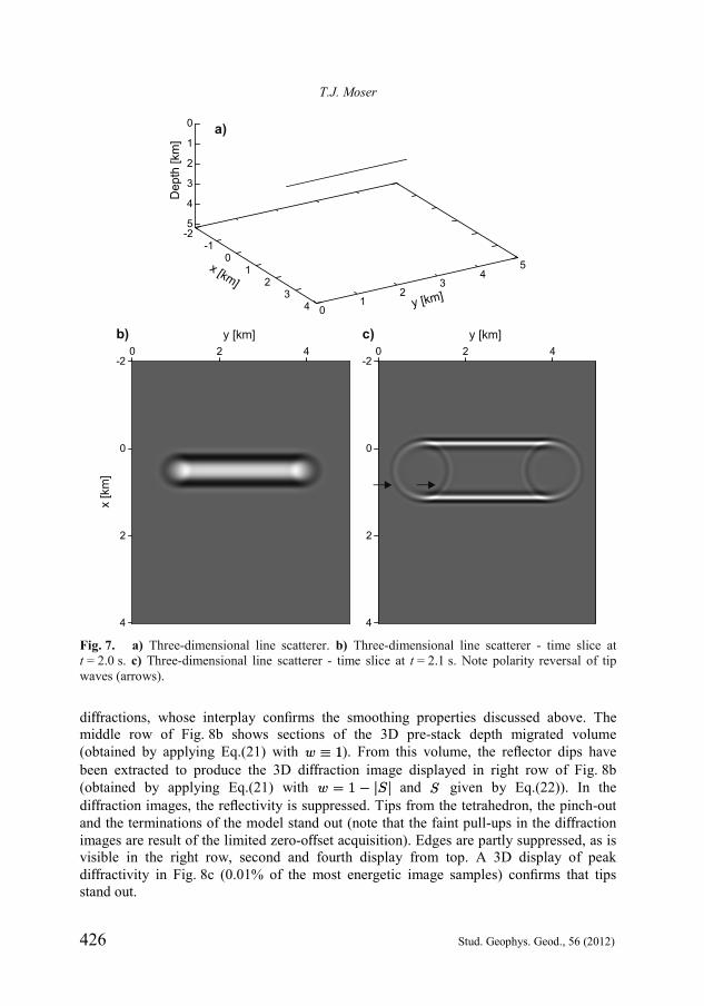
The line scatterer in three dimensions shown in Fig. 7a illustrates the smoothing properties of tip diffractions (although the non-specular diffraction from the line itself is not an edge diffraction, but rather a line diffraction). Here a source signal with central frequency 10 Hz has been chosen, and a (dense) acquisition consisting of 501 lines with 1001 common-mid points each. At the tips (or end points) of the line scatterer, tip waves
Fig. 5. Layer-fault model. a) Scatterer model; b) velocity model; c) section - note diffractions from scattering objects and fault points (left/right arrows).
0123456
0 2 4 6 8 10 12 14
a)
Distance [km]
Dep
th [k
m]
0
0 5 10 15
5
b)
Distance [km]
Dep
thkm [
]
km/s
2
4
0
0 5 10 15
5
c)
Distance [km]
Tim
e [s
]
Ray-Born for migration and diffraction analysis
Stud. Geophys. Geod., 56 (2012) 425
are generated which act as correctors to line diffraction. This is shown in the (zero-offset) time slices of Figs. 7b and 7c. In space (xx, yy , zz for t > 0t > 0) the line diffracted wave has the shape of a cylinder with the line as its axis. In time (xx, yy , tt for z > 0z > 0) it has the shape of a one-sheeted hyperbolic cylinder. At the time of excitation of the line scatterer (t = 2t = 2 s, Fig. 7b) a single line diffraction is visible in the time section. It has a smeared-out character because it is a section tangent to the apex of the hyperbolic cylinder. At t = 2:1t = 2:1 s (Fig. 7c) the two rectilinear branches of the hyperbolic cylinder of the line diffraction are visible, as well as the two tip diffractions. The tip diffractions are spherical waves in space so in time domain they are one-sheeted hyperboloids, with circles as time sections. As in the case of edge diffraction (Fig. 3e), the tip diffractions have a smoothing effect on the line diffractor response. Also they have the same corrective properties: there is a polarity reversal across the shadow boundary (arrows in Fig. 7c), the amplitude is half that of the line diffraction and the waveforms are equal.
The final example serves to illustrate the effect discussed in Section 6 and in Moser (2010b) on specularity suppression on 3D diffraction imaging. Consider Fig. 8a, consisting of a wedge with a tetrahedron-shaped body on top. The tetrahedron is similar to the pyramid-model of Klem-Musatov et al. (2008), the wedge is a commonly known challenge for seismic imaging (Moser and Howard, 2008). The reference velocity model is given by v = 1:5v = 1:5 km/s + 0:1z0:1z. Ray-Born modeling was used to generate 3D zero-offset synthetic data, the source signal has a central frequency of 5 Hz and coincident source/receiver points cover a regular grid of 201 × 201 points. Fig. 8b on the left shows the (zero-offset) data along four representative vertical sections; here reflections, edge and tip waves can be identified (note out-of-plane effects). In fact, detailed inspection of vertical sections and time slices (not shown here) reveals a rich pattern of edge and tip
Fig. 6. Salt dome model. a) Scatterer model; b) velocity model; c) section - note isolated diffraction from pinch-out and triplicated reflections disappearing to infinity (left/right arrows).
0123456
0 2 4 6 8 10 12 14
a)
Distance [km]
Dep
th [k
m]
0
0 5 10 15
5
b)
Distance [km]
Dep
thkm [
]
km/s
2
4
0
0 5 10 15
5
c)
Distance [km]
Tim
e [s
]
T.J. Moser
426 Stud. Geophys. Geod., 56 (2012)
diffractions, whose interplay confirms the smoothing properties discussed above. The middle row of Fig. 8b shows sections of the 3D pre-stack depth migrated volume (obtained by applying Eq.(21) with w ´ 1w ´ 1). From this volume, the reflector dips have been extracted to produce the 3D diffraction image displayed in right row of Fig. 8b (obtained by applying Eq.(21) with w = 1 ¡ jS jw = 1 ¡ jS j and SS given by Eq.(22)). In the diffraction images, the reflectivity is suppressed. Tips from the tetrahedron, the pinch-out and the terminations of the model stand out (note that the faint pull-ups in the diffraction images are result of the limited zero-offset acquisition). Edges are partly suppressed, as is visible in the right row, second and fourth display from top. A 3D display of peak diffractivity in Fig. 8c (0.01% of the most energetic image samples) confirms that tips stand out.
Fig. 7. a) Three-dimensional line scatterer. b) Three-dimensional line scatterer - time slice at t = 2.0 s. c) Three-dimensional line scatterer - time slice at t = 2.1 s. Note polarity reversal of tip waves (arrows).
-2-1
01
23
4 01
23
45
0
1
2
3
4
5
x [km]
y [km]
Dep
th [k
m]
a)
b)
-2
0
0
2
2
4
4
x [k
m]
y [km] c)
-2
0
0
2
2
4
4y [km]
Ray-Born for migration and diffraction analysis
Stud. Geophys. Geod., 56 (2012) 427
8. CONCLUDING REMARKS
The objective of the review of ray-Born forward modeling presented in this paper is multifold. First, it is to reconfirm the role of ray-Born modeling in depth migration. Most depth migration algorithms are based on a decomposition of the subsurface into a slowly varying background model and a rapidly varying scatterer. The background model is assumed to be known and suitable for (efficient and accurate) evaluation of Green’s functions; the scatterer is the unknown and the objective of the migration. With some provisions, the assumption that the background is slowly varying can be translated into the assumption that it is ray-tracing friendly. The common challenge of depth migration is to construct a background model that ensures an optimal focusing of the migrated image. An accurate background usually implies a weak scatterer and validates the first Born approximation for the scattered wave. The application of the ray-Born approximation in depth migration, explicit or implicit, is a justification by itself for considering it for forward modeling. Its theoretical justification is given by the convergence of the scattering series; in asymptotic sense (high-frequency limit for the ray component, weak-scattering limit for the scattering component) the ray-Born signal is exact.
The second objective of the paper is to recapitulate a number of properties of the ray-Born approximation for forward modeling and discuss implementation details. An important property is the fact that there are no assumptions on the smoothness of the scatterer, other than integrability. This means that scattering models of considerable complexity can be taken into account, in many cases models that pose serious difficulties for other forward modeling techniques, such as ray-tracing modeling. As soon as the Green’s functions in the background model are known and available, e.g. in the form of travel-time and amplitude tables, ray-Born modeling can be implemented as a simple volume integral over the scatterer.
Fig. 8a. Pinch-out/tetrahedron model.
24
68
10 -1 0 1 2 3 4 5 6
0.0
0.2
0.4
0.6
0.8
1.0
1.2
1.4
x [km]y [km]
Dep
th [k
m]
T.J. Moser
428 Stud. Geophys. Geod., 56 (2012)
Ray-Born modeling in its simplest implementation provides first-order scattering only, and therefore modeled data without multiples. In many cases, for instance for the purpose of generating test data for depth migration algorithms, this is an advantage. Multiple scattering can be included by extra integrations, but is computationally more expensive. Ray-Born modeling can be formulated for acoustic (P-wave) scattering; extensions to elastic and anisotropic media have been documented in the literature (see Červený, 2001, Section 2.6.2 for references).
The third objective of the paper is to make a case for ray-Born modeling as a simple tool for the modeling and analysis of diffractions. The scattering integral does not distinguish between specular reflections and non-specular diffractions. Therefore, if the integration is carried out accurately enough, reflections and diffractions are modeled with the same reliability. Despite its simplicity, this is a very powerful statement: as soon as ray-Born is found adequate for reflection modeling, it is, a forteriori, also adequate for diffraction modeling.
Simple examples show that ray-Born modeling generates caustic diffractions when the caustic is caused by an undulation of a smooth reflecting interface (Figs. 4c, 5c and 6c). Here the scattering integral has a smoothing effect, in contrast to standard ray theory which results in a singularity consisting of an infinite amplitude at the caustic and a shadow zone beyond it. The same smoothing effect occurs at edges and tips of smooth reflecting interfaces. Ray-Born modeling produces edge and tip diffractions with the same properties as predicted by edge and tip diffraction theory (Keller, 1962; Trorey, 1970; Klem-Musatov et al., 2008). Where an edge causes the reflection to terminate abruptly and to cast a shadow, the edge diffraction acts as a correction factor that ensures the
Fig. 8b. Zero-offset section, full-wave image and diffraction image (left, middle, right) over pinchout-tetrahedron model. Sections in x- and y-directions as indicated. Note tip diffraction images (right top to bottom) and image of the tetrahedron edge (bottom right along y = 3.2 km).
Tim
e [s
]
y-distance [km] y-distance [km] y-distance [km]
x-distance [km] x-distance [km] x-distance [km]
0 2 4 6 0 2 4 6 0 2 4 6
0 2 4 6 0 2 4 6 0 2 4 6
0 2 4 6 0 2 4 6 0 2 4 6
0 2 4 6 8 10 0 2 4 6 8 10 0 2 4 6 8 10
Tim
e [s
]Ti
me
[s]
Tim
e [s
]
0.5
1.5
2.5 Dep
th [k
m]
Dep
th [k
m]
Dep
th [k
m]
Dep
th [k
m]
0.60.81.01.2
0.60.81.01.2
0.60.81.01.2
0.60.81.01.2
Dep
th [k
m]
Dep
th [k
m]
Dep
th [k
m]
Dep
th [k
m]
0.60.81.01.2
0.60.81.01.2
0.60.81.01.2
0.60.81.01.2
0.5
1.5
2.5
0.5
1.5
2.5
0.5
1.5
2.5
x=2.0 km
x=4.0 km
x=5.5 km
y=3.2 km y=3.2 km y=3.2 km
x=2.0 km
x=4.0 km
x=5.5 km
x=2.0 km
x=4.0 km
x=5.5 km
Ray-Born for migration and diffraction analysis
Stud. Geophys. Geod., 56 (2012) 429
smoothness of the total wave field. At the shadow boundary, the edge diffraction has the same waveform but half the amplitude of the reflected wave; across the shadow boundary its polarity is reversed. At the end point of a diffracting edge, the tip diffraction has similar smoothing properties with respect to the edge diffraction.
The fact that edge and tip diffractions properties are correctly reproduced by ray-Born modeling has useful applications for the analysis of diffractions and their relation to structural geology. For an important part, the diffraction response of three-dimensional structural complexities, such as faults and fractures, is still unexplored terrain and several phenomena are not yet fully explained. Pelissier et al. (2011) give some examples of three-dimensional diffraction analysis on a Ground Penetrating Radar data set with the objective to obtain a character match of diffractions modeled on simple features with diffractions observed in the data. If such simple features can be classified into elementary building blocks, or templates, of diffractors and their response, more complicated responses can be understood in terms of these templates. A next step is the inversion of diffraction response, i.e. the extraction of structural parameters from observed diffractions. Notably, in the GPR data set studied by Pelissier et al. (2011), reflections and reflectivity hardly play any role and the background model is very simple (almost constant). Examples pointing to the inversion of diffractions are given by Landa and Maximov (1980) and Landa and Gurevich (1998). As suggested by the review and examples of this paper, ray-Born modeling can play an important role in the efficient and target-oriented generation of diffraction response of trial models. The same considerations apply to diffraction imaging. Here the forward modeling of diffractions is crucial for the understanding and interpretation of diffraction images. As pointed out in this paper, reflections, edge-and tip diffractions can be classified according to topological properties. In Moser (2011) it is argued that these properties have their implications on reflection, edge-and tip diffraction imaging. The specularity suppression used in diffraction imaging (i.e., Eq.(21) with w = 1 ¡ jS jw = 1 ¡ jS j and SS given by Eq.(22)) has the effect of a full suppression of the reflection image, a partial suppression of the edge diffraction image and almost no
Fig. 8c. Diffractivity (maximum diffraction image energy) on pinchout-tetrahedron model.
0.0
0.2
0.4
0.6
0.8
1.0
1.2
1.42
46
810
x [km]-1 0 1 2 3 4 5 6
y [km]
Dep
th [k
m]
T.J. Moser
430 Stud. Geophys. Geod., 56 (2012)
suppression of the tip diffraction image. As a result, edge images constitute the skeleton of a structural model and tip images indicate the joints of the skeleton (Figs. 8b,c attempt to illustrate this).
This paper does not pretend to make rigorous claims and several arguments in it can be further developed. All presented examples concern acquisitions with coincident source and receiver locations. Evidently, offset dependance of ray-Born signals adds another dimension to analysis and interpretation, in particular of edge and tip diffractions (offset-dependent diffractivity), but also of standard offset-dependent reflectivity (Weglein et al. 2003; Nita et al., 2004). While advocating the advantages of ray-Born modeling, it must be kept in mind that there are certain limitations. Most importantly, a multivalued ray field in a complicated background poses difficulties. With respect to diffraction modeling, the question of whether all types of diffractions can be modeled using the ray-Born approximation is beyond the scope of the paper. For instance, surface diffractions (such as creeping waves around convex bodies, see Keller, 1962) are not covered by the implementations described here.
Acknowledgments: The author thanks Dr Arkady Aizenberg, Reda Baina, Mark Grasmueck,
Henk Keers, Shmoriahu Keydar, Prof. K. Klem-Musatov, Dirk Kraaijpoel, Evgeny Landa, Dmitri Lokshtanov, Jan Pajchel, Michael Pelissier, Gennady Ryzhikov, and Constantine Tsingas for discussions (but view points taken in this paper are the responsibility of the author). Doug Angus, James Hobro, Ivan Pšenčík, and Colin Thomson are thanked for their review.
References
Beydoun W. and Mendes M., 1989. Elastic Ray-Born l2 migration/inversion. Geophys. J. Int., 97, 151160.
Beydoun W. and Tarantola A., 1988. First Born and Rytov approximations: Modeling and inversion conditions in a canonical example. J. Acoust. Soc. Am., 83, 10451055.
Beylkin G. and Burridge R., 1990. Linearized inverse scattering problems in acoustics and elasticity. Wave Motion, 12, 1552.
Červený V., 2001. Seismic Ray Theory. Cambridge University Press, Cambridge, U.K.
Červený V. and Coppoli A.D.M., 1992. Ray-Born synthetic seismograms for complex structures containing scatterers. J. Seism. Explor., 1, 191206.
Chapman C.H., 2004. Fundamentals of Seismic Wave Propagation. Cambridge University Press, Cambridge, U.K.
Keller J.B., 1962. A geometrical theory of diffraction. J. Opt. Soc. Am., 52, 116130.
Keller J.B., 1969. Accuracy and validity of the Born and Rytov approximations. J. Opt. Soc. Am., 59, 10031004.
Khaidukov V.G., 1982. Calculation of the scalar wave field scattered by a sphere and analysis of the images. Geologiya i Geofizika, 23, 104114 (in Russian).
Ray-Born for migration and diffraction analysis
Stud. Geophys. Geod., 56 (2012) 431
Khaidukov V., Landa E. and Moser T.J., 2004. Diffraction imaging by focusing-defocusing: An outlook on seismic superresolution. Geophysics, 69, 14781490.
Klem-Musatov K., Aizenberg A., Pajchel J. and Helle H.B., 2008. Edge and Tip Diffractions: Theory and Applications in Seismic Prospecting. SEG Geophysical Monograph Series, 14. Society of Exploration Geophysicists, Tulsa, OK.
Kravtsov A. and Orlov Yu.I., 1993. Caustics, Catastrophes and Wave Fields. Springer-Verlag, Berlin, Germany.
Lambaré G., Lucio P.S. and Hanyga A., 1996. Two-dimensional multivalued traveltime and amplitude maps by uniform sampling of a ray field. Geophys. J. Int., 125, 584598.
Landa E. and Maximov A., 1980. Testing of algorithm for low-amplitude fault detection. Geology and Geophysics, 12, 108113 (in Russian).
Landa E. and Gurevich B., 1998. Interference pattern as a means of fault detection. The Leading Edge, 17, 752757.
Moser T.J., 1997. Influence of realistic backgrounds on the validity of ray/Born inversion. J. Seism. Explor., 6, 239252.
Moser T.J., 2009. Diffraction imaging in subsalt geometries and a new look at the scope of reflectivity. Extended Abstract. EAGE Subsalt Imaging Workshop, European Association of Geoscientists & Engineers, Houten, The Netherlands.
Moser T.J., 2010a. Dip extraction from three-dimensional depth images - algorithms and applications. Extended Abstract. EAGE Conference St. Petersburg, European Association of Geoscientists & Engineers, Houten, The Netherlands.
Moser T.J., 2010b. Review of ray-Born forward modeling for migration. Extended Abstract. EAGE Conference Barcelona, European Association of Geoscientists & Engineers, Houten, The Netherlands.
Moser T.J., 2011. Edge and tip diffraction imaging in three dimensions. Extended Abstract. EAGE Conference Vienna, European Association of Geoscientists & Engineers, Houten, The Netherlands.
Moser T.J. and Howard C.B., 2008. Diffraction imaging in depth. Geophys. Prospect., 56, 627641.
Natterer F., 2004. Error estimates for the Born approximation. Inverse Probl., 20, 447452.
Nita B.G., Matson K.N. and Weglein A.B., 2004. Forward scattering series and seismic events: far field approximations, critical and postcritical events. SIAM J. Appl. Math., 64, 21672185.
Pelissier M., Moser T.J., Pajchel J. and Grasmueck M., 2011. Modeling and observation of the 3D diffraction response of faults and fractures. Extended Abstract. EAGE Conference Vienna, European Association of Geoscientists & Engineers, Houten, The Netherlands.
Reshef M. and Landa E., 2009. Poststack velocity analysis in the dip-angle domain using diffractions. Geophys. Prospect., 57, 811821.
Rudin W., 1966. Real and Complex Analysis. McGraw-Hill. New York.
Santos L.T., Schleicher J., Tygel M. and Hubral P., 2000. Seismic modeling by demigration. Geophysics, 65, 12811289.
Sethian J.A., 1996. Level Set Methods. Cambridge University Press, Cambridge, U.K.
T.J. Moser
432 Stud. Geophys. Geod., 56 (2012)
Tarantola A., 1984. Linearized inversion of seismic reflection data. Geophys. Prospect., 32, 9981015.
Trorey A.W., 1970. A simple theory for seismic diffractions. Geophysics, 35, 762784.
Vinje V., Iversen E. and Gjøystdal H., 1993. Traveltime and amplitude estimation using wavefront construction. Geophysics, 58, 11571166.
Weglein A.B., Arajo F.V., Carvalho P.M., Stolt R.H., Matson K.M., Coates R.T., Corrigan D., Foster D.J., Shaw S.A. and Zhang H., 2003. Inverse scattering series and seismic exploration, Inverse Probl., 19, R27R83.