Renewable and Sustainable Energy Reviews 18 (2013) 568–582

Contents lists available at SciVerse ScienceDirect

Renewable and Sustainable Energy Reviews

1364-03

http://d

n Corr

Tel.: þ6

E-m

journal homepage: www.elsevier.com/locate/rser

Review of transmission schemes and case studies for renewable powerintegration into the remote grid

Kazi Nazmul Hasan a,b, Tapan Kumar Saha a,b,n, Mehdi Eghbal a,b, Deb Chattopadhyay b

a Queensland Geothermal Energy Centre of Excellence, University of Queensland, St. Lucia, Brisbane, QLD 4072, Australiab School of ITEE, University of Queensland, St. Lucia, Brisbane, QLD 4072, Australia

a r t i c l e i n f o

Article history:

Received 24 April 2012

Received in revised form

25 October 2012

Accepted 27 October 2012Available online 30 November 2012

Keywords:

Cost–benefit analysis

Location constrained generation

Net market benefit

Renewable power integration

Transmission investment framework

21/$ - see front matter & 2012 Elsevier Ltd. A

x.doi.org/10.1016/j.rser.2012.10.045

esponding author at: Queensland Geotherma

1 733 653962; fax: þ61 733 654999.

ail address: saha@itee.uq.edu.au (T.K. Saha).

a b s t r a c t

Investment in transmission for renewable power penetration to the remote grid essentially faces a set of

inherent, regulatory, economic and technical challenges. This work investigates these challenges to

enhance renewable power integration into the remote grid. This study aims to enhance regulatory

policies and associated planning frameworks to be more efficient and justifiable for renewable power

integration paradigm. First, a set of leading transmission schemes practiced, or investigated, in different

countries are evaluated against the challenges which are obvious for long distance renewable power

transmission. Second, a net benefit framework is presented to address the challenging issues of location

constrained renewable power penetration into the Queensland network of the Australian grid. The

proposed framework incorporates the carbon emission price as an environmental benefit which

significantly influences the cost–benefit analysis. This paper discusses the ‘hub approach’ of network

integration. The transmission investment cost allocation is addressed here as well. The concepts are

verified through the implementation of the proposed framework in four prospective projects of the

Queensland network in the Australian national electricity market (NEM).

& 2012 Elsevier Ltd. All rights reserved.

Contents

1. Introduction . . . . . . . . . . . . . . . . . . . . . . . . . . . . . . . . . . . . . . . . . . . . . . . . . . . . . . . . . . . . . . . . . . . . . . . . . . . . . . . . . . . . . . . . . . . . . . . . . . . . . . 569

2. Challenges of renewable power penetration to remote grid . . . . . . . . . . . . . . . . . . . . . . . . . . . . . . . . . . . . . . . . . . . . . . . . . . . . . . . . . . . . . . . . 569

2.1. Inherent challenges . . . . . . . . . . . . . . . . . . . . . . . . . . . . . . . . . . . . . . . . . . . . . . . . . . . . . . . . . . . . . . . . . . . . . . . . . . . . . . . . . . . . . . . . . . 570

2.2. Regulatory and economic challenges . . . . . . . . . . . . . . . . . . . . . . . . . . . . . . . . . . . . . . . . . . . . . . . . . . . . . . . . . . . . . . . . . . . . . . . . . . . . 570

2.3. Technical challenges . . . . . . . . . . . . . . . . . . . . . . . . . . . . . . . . . . . . . . . . . . . . . . . . . . . . . . . . . . . . . . . . . . . . . . . . . . . . . . . . . . . . . . . . . 570

3. Review of transmission schemes to meet the challenges of renewable power integration into the remote grid . . . . . . . . . . . . . . . . . . . . . . . 571

3.1. Regulatory investment test for transmission (RIT-T) [24] . . . . . . . . . . . . . . . . . . . . . . . . . . . . . . . . . . . . . . . . . . . . . . . . . . . . . . . . . . . . 571

3.2. Scale efficient network extension (SENE) [9,23] . . . . . . . . . . . . . . . . . . . . . . . . . . . . . . . . . . . . . . . . . . . . . . . . . . . . . . . . . . . . . . . . . . . . 572

3.3. Victorian generation clusters’ connection (VGCC) [11]. . . . . . . . . . . . . . . . . . . . . . . . . . . . . . . . . . . . . . . . . . . . . . . . . . . . . . . . . . . . . . . 572

3.4. Transmission investment incentives (by OFGEM) [12] . . . . . . . . . . . . . . . . . . . . . . . . . . . . . . . . . . . . . . . . . . . . . . . . . . . . . . . . . . . . . . . 572

3.5. Strategic transmission investment plan (by CEC) [14] . . . . . . . . . . . . . . . . . . . . . . . . . . . . . . . . . . . . . . . . . . . . . . . . . . . . . . . . . . . . . . . 573

3.6. Location constrained resource interconnection (LCRI) [13] . . . . . . . . . . . . . . . . . . . . . . . . . . . . . . . . . . . . . . . . . . . . . . . . . . . . . . . . . . . 573

4. Net market benefit evaluation approach. . . . . . . . . . . . . . . . . . . . . . . . . . . . . . . . . . . . . . . . . . . . . . . . . . . . . . . . . . . . . . . . . . . . . . . . . . . . . . . . 573

4.1. Evaluation of market benefit . . . . . . . . . . . . . . . . . . . . . . . . . . . . . . . . . . . . . . . . . . . . . . . . . . . . . . . . . . . . . . . . . . . . . . . . . . . . . . . . . . . 573

4.1.1. OPF formulation . . . . . . . . . . . . . . . . . . . . . . . . . . . . . . . . . . . . . . . . . . . . . . . . . . . . . . . . . . . . . . . . . . . . . . . . . . . . . . . . . . . . . . 573

4.1.2. Producer surplus . . . . . . . . . . . . . . . . . . . . . . . . . . . . . . . . . . . . . . . . . . . . . . . . . . . . . . . . . . . . . . . . . . . . . . . . . . . . . . . . . . . . . 574

4.1.3. Consumer surplus . . . . . . . . . . . . . . . . . . . . . . . . . . . . . . . . . . . . . . . . . . . . . . . . . . . . . . . . . . . . . . . . . . . . . . . . . . . . . . . . . . . . 574

4.1.4. Merchandizing surplus. . . . . . . . . . . . . . . . . . . . . . . . . . . . . . . . . . . . . . . . . . . . . . . . . . . . . . . . . . . . . . . . . . . . . . . . . . . . . . . . . 574

4.1.5. Emission tax . . . . . . . . . . . . . . . . . . . . . . . . . . . . . . . . . . . . . . . . . . . . . . . . . . . . . . . . . . . . . . . . . . . . . . . . . . . . . . . . . . . . . . . . . 574

4.1.6. LRET benefit . . . . . . . . . . . . . . . . . . . . . . . . . . . . . . . . . . . . . . . . . . . . . . . . . . . . . . . . . . . . . . . . . . . . . . . . . . . . . . . . . . . . . . . . . 574

4.2. Cost considerations . . . . . . . . . . . . . . . . . . . . . . . . . . . . . . . . . . . . . . . . . . . . . . . . . . . . . . . . . . . . . . . . . . . . . . . . . . . . . . . . . . . . . . . . . . 574

4.3. Payback scheme and cost recovery mechanism . . . . . . . . . . . . . . . . . . . . . . . . . . . . . . . . . . . . . . . . . . . . . . . . . . . . . . . . . . . . . . . . . . . . 574

ll rights reserved.

l Energy Centre of Excellence, University of Queensland, Staff House Road, St. Lucia, Brisbane, QLD 4072, Australia.

K.N. Hasan et al. / Renewable and Sustainable Energy Reviews 18 (2013) 568–582 569

5. Case studies . . . . . . . . . . . . . . . . . . . . . . . . . . . . . . . . . . . . . . . . . . . . . . . . . . . . . . . . . . . . . . . . . . . . . . . . . . . . . . . . . . . . . . . . . . . . . . . . . . . . . . 575

5.1. Queensland network . . . . . . . . . . . . . . . . . . . . . . . . . . . . . . . . . . . . . . . . . . . . . . . . . . . . . . . . . . . . . . . . . . . . . . . . . . . . . . . . . . . . . . . . . 575

5.2. Case studies overview . . . . . . . . . . . . . . . . . . . . . . . . . . . . . . . . . . . . . . . . . . . . . . . . . . . . . . . . . . . . . . . . . . . . . . . . . . . . . . . . . . . . . . . . 575

5.2.1. Kennedy Wind Farm (700 MW, 290 km) [37] . . . . . . . . . . . . . . . . . . . . . . . . . . . . . . . . . . . . . . . . . . . . . . . . . . . . . . . . . . . . . . . 575

5.2.2. Copper String Project (400 MW, 720 km) [38] . . . . . . . . . . . . . . . . . . . . . . . . . . . . . . . . . . . . . . . . . . . . . . . . . . . . . . . . . . . . . . 576

5.2.3. Cooper Basin Geothermal (2000 MW, 1000 km) [39] . . . . . . . . . . . . . . . . . . . . . . . . . . . . . . . . . . . . . . . . . . . . . . . . . . . . . . . . . 576

5.2.4. PNG Hydro (1800 MW, 250 km cableþ200 km) . . . . . . . . . . . . . . . . . . . . . . . . . . . . . . . . . . . . . . . . . . . . . . . . . . . . . . . . . . . . . 576

5.3. Wind power sensitivity . . . . . . . . . . . . . . . . . . . . . . . . . . . . . . . . . . . . . . . . . . . . . . . . . . . . . . . . . . . . . . . . . . . . . . . . . . . . . . . . . . . . . . . 576

6. Analytical results . . . . . . . . . . . . . . . . . . . . . . . . . . . . . . . . . . . . . . . . . . . . . . . . . . . . . . . . . . . . . . . . . . . . . . . . . . . . . . . . . . . . . . . . . . . . . . . . . . 576

6.1. Producer surplus . . . . . . . . . . . . . . . . . . . . . . . . . . . . . . . . . . . . . . . . . . . . . . . . . . . . . . . . . . . . . . . . . . . . . . . . . . . . . . . . . . . . . . . . . . . . 576

6.2. Consumer surplus . . . . . . . . . . . . . . . . . . . . . . . . . . . . . . . . . . . . . . . . . . . . . . . . . . . . . . . . . . . . . . . . . . . . . . . . . . . . . . . . . . . . . . . . . . . 578

6.3. Merchandizing surplus. . . . . . . . . . . . . . . . . . . . . . . . . . . . . . . . . . . . . . . . . . . . . . . . . . . . . . . . . . . . . . . . . . . . . . . . . . . . . . . . . . . . . . . . 578

6.4. Carbon emission tax. . . . . . . . . . . . . . . . . . . . . . . . . . . . . . . . . . . . . . . . . . . . . . . . . . . . . . . . . . . . . . . . . . . . . . . . . . . . . . . . . . . . . . . . . . 578

6.5. LRET payment . . . . . . . . . . . . . . . . . . . . . . . . . . . . . . . . . . . . . . . . . . . . . . . . . . . . . . . . . . . . . . . . . . . . . . . . . . . . . . . . . . . . . . . . . . . . . . 578

6.6. Net market benefit . . . . . . . . . . . . . . . . . . . . . . . . . . . . . . . . . . . . . . . . . . . . . . . . . . . . . . . . . . . . . . . . . . . . . . . . . . . . . . . . . . . . . . . . . . . 578

6.7. Payback scheme . . . . . . . . . . . . . . . . . . . . . . . . . . . . . . . . . . . . . . . . . . . . . . . . . . . . . . . . . . . . . . . . . . . . . . . . . . . . . . . . . . . . . . . . . . . . . 579

6.8. Wind power sensitivity . . . . . . . . . . . . . . . . . . . . . . . . . . . . . . . . . . . . . . . . . . . . . . . . . . . . . . . . . . . . . . . . . . . . . . . . . . . . . . . . . . . . . . . 580

7. Conclusions . . . . . . . . . . . . . . . . . . . . . . . . . . . . . . . . . . . . . . . . . . . . . . . . . . . . . . . . . . . . . . . . . . . . . . . . . . . . . . . . . . . . . . . . . . . . . . . . . . . . . . 580

Acknowledgements . . . . . . . . . . . . . . . . . . . . . . . . . . . . . . . . . . . . . . . . . . . . . . . . . . . . . . . . . . . . . . . . . . . . . . . . . . . . . . . . . . . . . . . . . . . . . . . . . . . . 581

Appendix . . . . . . . . . . . . . . . . . . . . . . . . . . . . . . . . . . . . . . . . . . . . . . . . . . . . . . . . . . . . . . . . . . . . . . . . . . . . . . . . . . . . . . . . . . . . . . . . . . . . . . . . 581

References . . . . . . . . . . . . . . . . . . . . . . . . . . . . . . . . . . . . . . . . . . . . . . . . . . . . . . . . . . . . . . . . . . . . . . . . . . . . . . . . . . . . . . . . . . . . . . . . . . . . . . . . . . . 581

1. Introduction

Due to the combined effects of restructuring, environmentalconcerns and emission trading schemes, the electricity marketworldwide is experiencing a shifting trend in generation portfolioand real time dispatch [1,2]. Adequate transmission infrastructureand a suitable investment scheme to meet the evolving marketstructure has emerged as a critical need to meet the newgeneration investment and dispatch pattern. Consequently, thegeneration shift and transmission investment bring many tech-nical and economic challenges for planning and operation ofelectricity markets that need to be addressed through develop-ment of new analytical approaches, e.g., [3].

Looking at some of the market specific experiences, challengesof renewable transmission investment and regulatory amend-ments for the UK, Brazil and Chilean grids are reported in [4]. Inaddition, the problems of the USA grid for large scale renewablepower integration are discussed in [5]. Some potential discussionof possible avenues to contemplate efficient planning has alsobeen identified in that study. In another work, Swider et al. [6]presented the transmission cost allocation issues in sevenEuropean countries and discussed conditions and barriers topromote renewable power integration to a remote grid. In adetailed study, Great Britain’s practice to employ a new transmis-sion pricing method is presented in [7]. That study also consid-ered four scenarios of the GB electricity network, around the2020 ‘FutureNet’ program including the transmission cost sensi-tivity on generation, demand and network topology. The strate-gies of the Spanish electricity grid reform is reported in [1], thatincludes inter alia combinations of load conditions, generationprofile and network status. Amendments for planning and build-ing large scale transmission networks in Brazil are discussedin [8] that highlight the technical, economic and regulatorychallenges.

The regulatory investment test for transmission (RIT-T) is usedin the Australian national electricity market (NEM) as the centralmechanism to decide transmission investment that includes anexplicit cost–benefit test and assessment of market benefit oftransmission. While it has a number of attractive features, italso has some shortcoming when it comes to large scale renew-able power integration to the grid from a remote location [9].Although the scale efficient network extension (SENE) was pro-mulgated by the Australian Energy Market Commission for theAustralian NEM to get around the transmission investment issues,

the scheme was subsequently dropped citing implementationdifficulties [10]. Also a low emission generation enhancing trans-mission scheme is proposed in the NEM for the Victorian genera-tion clusters’ connection (VGCC) [11]. In the UK electricity market,the Office of Gas and Electricity Market (OFGEM) has introduced ascheme to provide incentives to transmission projects based onthe available renewable resources, appropriate constraint costsand required investments [12]. In the California ISO, a specialarrangement for remote renewable generator connections isreported known as the ‘location constrained resource interconnec-

tion’ [13]. The California Energy Commission proposes a ‘strategic

transmission investment plan’ to promote environment driventransmission expansion [14]. Details of these transmissionschemes are discussed in a later section. Investigations throughall of the relevant studies affirm the need for an efficientregulatory framework, economic model, network structure andmarket response to mitigate the renewable power integrationchallenges [15].

In order to address the renewable power integration issuescomprehensively, planners need to develop a proper analyticalframework to adequately deal with the challenges that large scalerenewable resources present. This study aims to develop such aframework in the Australian context and in particular highlightsthe impact and potential of remote transmission investments onthe net market benefit. Four case studies have been presentedthat focus on proposed long distance renewable power integra-tion into the Queensland electricity network.

The rest of the paper is organized as follows. Section 2 presentsthe challenges of renewable power penetration to the remotegrid, followed by a review of some leading transmission schemesto meet those challenges in Section 3. A net market benefitframework is described in Section 4 followed by Section 5 thatdeals with case studies of four prospective large scale renewablepower projects to be connected to the Australian Queensland

network. Analytical results and conclusions are presented inSections 6 and 7, respectively.

2. Challenges of renewable power penetration to remote grid

Renewable power penetration from remote location constrainedgenerators to the grid is facing a set of challenges. Those challengesare categorized here as inherent, regulatory, economic and technicalaspects.

Nomenclature

ai,bi,ci Cost coefficients of generator i

Capi Capacity of generator i (MW)CSi

d Consumer surplus earned by consumer i ($)CSi0

d Consumer surplus before augmentation ($)d Demand (used as subscript)Ei Amount of CO2 produced by generator i (ton)Ff Branch flow at ‘for end’ (MW)Ft Branch flow at ‘to end’ (MW)Fmax Maximum limit of branch flow (MW)f i

p Cost function of generator i

g Generator (used as subscript)nd Number of load setng Number of generator setpbus Real power of a bus (MW)Qbus Reactive power of a bus (MVAR)pd Real power of the load (MW)Qd Reactive power of the load (MVAR)

pid Power consumed by load i (MW)

pig Power produced by generator i (MW)

PCig Producer cost incurred by generator i ($)

PRig Producer revenue earned by generator i ($)

PSig Producer surplus earned by generator i ($)

r Discount ratet Time span (hour)Vm Voltage magnitude (Volt)y Number of yearslk Locational marginal price (LMP) at bus k ($/MWh)li

g LMP at generator bus, for generator i ($/MWh)li

d LMP at load bus for load i ($/MWh)fi

g Generation cost of generator i ($/MWh)ci Amount of renewable generation from generator

i (MW)pco2

Emission cost ($/ton CO2)s LRET payment ($/MWh)y Voltage angle

K.N. Hasan et al. / Renewable and Sustainable Energy Reviews 18 (2013) 568–582570

2.1. Inherent challenges

Inherent challenges are the uncertainty in generation and demand,balance between generation and demand and free rider problem.Significant generation expansion and demand growth in differentparts of the network causes major uncertainty in transmissionplanning. Uncertainty in the planning horizon can be categorized intwo aspects—probabilistic and possibilistic [16]. Probabilistic meth-ods are applicable to stochastic parameters which follow a probabilitydistribution, i.e., wind power follows a Weibull distribution. Alter-natively possibilistic approach is preferable to non stochastic para-meters, i.e., electrical load, installed capacity and controllablegenerators do not follow any probability distribution [17]. A systemplanning model requires these uncertainty considerations to addressthe practical issues appropriately [18–21]. However, as the primefocus of this paper is regulatory and economic aspects, detaileddiscussion of uncertainty modelling is reduced to limit the scope ofthe paper.

Another aspect of the challenge is the ‘‘chicken and egg’’

dilemma, i.e., which should come first—generation, or transmis-sion. A generator needs to be assured that there are adequatetransmissions facilities. On the other hand, transmission investorsneed firm generation expansion projects to ensure a certain levelof utilisation of the transmission assets [8]. A generator paying fortransmission upfront also faces the first mover disadvantage.Moreover, once the first generator builds a transmission line tobe connected to the network, network sharing and cost allocationbecomes contentious when any other generator is to be con-nected to the existing transmission corridor [6,9].

2.2. Regulatory and economic challenges

Another fundamental challenge of connecting remote location

constrained renewable resources to the grid is to endure theregulatory investment test and cost–benefit assessment policies.The shortfall of long distance remote transmission is theunderlying high investment cost [15]. A high investment dispro-portionate to the quantified benefits of the long distancetransmission may defer, or abandon, the grid integration[22]. In this regard, accumulation of strategic benefits of networkaugmentation is a critical issue to justify large initial invest

Economic challenges include the economies of scale and compe-tition with conventional generation sources. The economicaspects also address the transmission investment cost allocation

and transmission cost recovery. Cost allocation issues havereceived significant attention due to the fact that the transmissioncost of connecting remote renewable power is significant com-pared to connecting conventional power stations [9]. Hence,achieving the economies of scale in this prospect is a highlydecisive factor [8,15]. Further, remote location constrainedrenewable resources compete with nearby conventional powerplants to pass the economic tests [8].

Some challenges which fall both in the regulatory and economic

regimes are stranding asset risk, capturing strategic benefits,transmission investment cost allocation and (deep, shallowor hybrid) cost burden on generators [6,9]. Regulatory policiesdo not facilitate the recovery of costs of over built transmis-sion infrastructures [2], particularly if the transmission infra-structure is developed and no/little generation eventuatesthen the investment is at risk of being stranded. Traditionalregulatory frameworks fail to capture some unquantifiable ben-efits which are obtained through renewable generation entryto the electricity market [4]. Although the societal benefit ofscale efficient transmission is well understood, the issue of costallocation poses a significant hurdle [9]. Moreover, the remunera-tion of renewable transmission investment through the transmis-

sion use of system charges is still an emergent issue [8].

2.3. Technical challenges

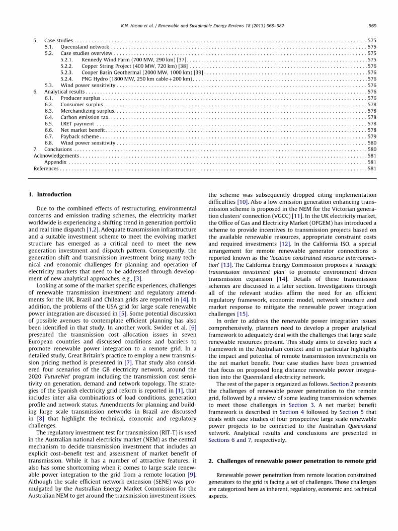
Technical challenges address the connection topology (spa-ghetti network or hub connection) and connection technology(HVAC, HVDC). Every generator of a remote generation cluster canbe connected to the grid on its own which creates the so calledspaghetti network as shown in Fig. 1a. For location constrained

remote generation resources this type of connection is not efficientand economic [9,15]. Rather, a high voltage transmission line canconnect the remote generation zone to load centres, wheresuccessive generators can be connected to the high capacity lineas shown in Fig. 1b. This is known as the scale efficient networkextension (SENE) framework [23]. Another option could beto establish a hub in the SENE approach as shown in Fig. 1c.The location of the hub would be decided based on the marketoperator’s policy. Regarding the transmission technology, if thereare a few thousands of MW of generation at a specific location,then an extra high-voltage (i.e., 800 kV) HVDC line could bejustifiable [8]. However, the possibility of staged developmentor tapping in between the transmission corridor can play an

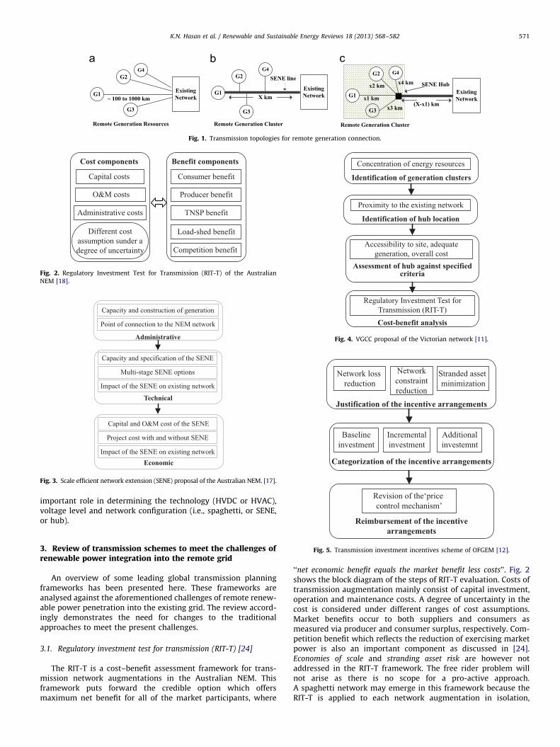
Identification of generation clusters

Concentration of energy resources

Assessment of hub against specifiedcriteria

Accessibility to site, adequategeneration, overall cost

Identification of hub location

Proximity to the existing network

Cost-benefit analysis

Regulatory Investment Test forTransmission (RIT-T)

Fig. 4. VGCC proposal of the Victorian network [11].Administrative

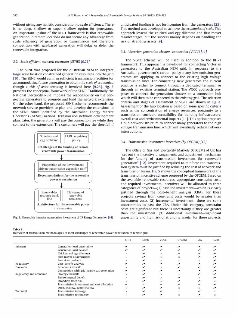
Capacity and construction of generation

Economic

Technical

Capacity and specification of the SENE

Point of connection to the NEM network

Multi-stage SENE options

Capital and O&M cost of the SENE

Project cost with and without SENE

Impact of the SENE on existing network

Impact of the SENE on existing network

Fig. 3. Scale efficient network extension (SENE) proposal of the Australian NEM. [17].

Justification of the incentive arrangements

Network lossreduction

Networkconstraintreduction

Stranded assetminimization

Categorization of the incentive arrangements

Baselineinvestment

Incrementalinvestment

Additionalinvestemnt

Reimbursement of the incentive

Revision of the‘pricecontrol mechanism’

Capital costs

Cost components

O&M costs

Administrative costs

Different costassumption sunder adegree of uncertainty

Consumer benefit

Benefit components

Producer benefit

TNSP benefit

Load-shed benefit

Competition benefit

Fig. 2. Regulatory Investment Test for Transmission (RIT-T) of the Australian

NEM [18].

Fig. 1. Transmission topologies for remote generation connection.

K.N. Hasan et al. / Renewable and Sustainable Energy Reviews 18 (2013) 568–582 571

important role in determining the technology (HVDC or HVAC),voltage level and network configuration (i.e., spaghetti, or SENE,or hub).

arrangements

Fig. 5. Transmission investment incentives scheme of OFGEM [12].

3. Review of transmission schemes to meet the challenges ofrenewable power integration into the remote grid

An overview of some leading global transmission planningframeworks has been presented here. These frameworks areanalysed against the aforementioned challenges of remote renew-able power penetration into the existing grid. The review accord-ingly demonstrates the need for changes to the traditionalapproaches to meet the present challenges.

3.1. Regulatory investment test for transmission (RIT-T) [24]

The RIT-T is a cost–benefit assessment framework for trans-mission network augmentations in the Australian NEM. Thisframework puts forward the credible option which offersmaximum net benefit for all of the market participants, where

‘‘net economic benefit equals the market benefit less costs’’. Fig. 2shows the block diagram of the steps of RIT-T evaluation. Costs oftransmission augmentation mainly consist of capital investment,operation and maintenance costs. A degree of uncertainty in thecost is considered under different ranges of cost assumptions.Market benefits occur to both suppliers and consumers asmeasured via producer and consumer surplus, respectively. Com-petition benefit which reflects the reduction of exercising marketpower is also an important component as discussed in [24].Economies of scale and stranding asset risk are however notaddressed in the RIT-T framework. The free rider problem willnot arise as there is no scope for a pro-active approach.A spaghetti network may emerge in this framework because theRIT-T is applied to each network augmentation in isolation,

K.N. Hasan et al. / Renewable and Sustainable Energy Reviews 18 (2013) 568–582572

without giving any holistic consideration to scale efficiency. Thereis no deep, shallow or super shallow option for generators.An important upshot of the RIT-T framework is that renewablegeneration in remote locations do not secure any advantage fromscale efficiency of generation or transmission and thereforecompetition with gas-based generation will delay or defer therenewable integration.

3.2. Scale efficient network extension (SENE) [9,23]

The SENE was proposed for the Australian NEM to integratelarge scale location constrained generation resources into the grid[10]. The SENE would confirm sufficient transmission facilities foraccommodating future generation to obtain the scale of economies,though a risk of asset standing is involved here [9,25]. Fig. 3presents the conceptual framework of the SENE. Traditionally theNational Electricity Rule imposes the responsibility on the con-necting generators to promote and fund the network extension.On the other hand, the proposed SENE scheme recommends thenetwork service providers to plan and develop the extensions tothe SENE zones identified by the Australian Energy MarketOperator’s (AEMO) national transmission network developmentplan. Later, the generators will pay the connection fee while theyconnect to the extensions. The customers will pay the shortfall if

Challenges of the funding of remoterenewable power transmission

‘Chicken andegg problem’

FERC regulatorypolicy

Architecture for the renewable powertransmission

Renewable-resource trunk

line

Clustering ofrenewableresources

Recommendations for the renewablepower transmission

Proposition of the Environmentdriven transmission expansion tariff

Fig. 6. Renewable intensive transmission investment of CA Energy Commission [14].

Table 1Overview of transmission methodologies to meet challenges of renewable power pene

Inherent Generation-load uncertainty

Generation-load balance

Chicken and egg dilemma

First mover disadvantages

Free rider problem

Regulatory Cost–benefit analysis

Economic Economies of scale

Competition with grid-nearby gas generation

Regulatory and economic Strategic benefits

Environmental benefit

Stranding asset risk

Transmission investment and cost allocation

Deep, shallow, super-shallow

Technical Transmission topology

Transmission technology

anticipated funding is not forthcoming from the generators [25].This method was developed to achieve the economies of scale. Thisapproach lessens the chicken and egg dilemma and first moverdisadvantages, but the success mainly depends on handling therisk of stranding assets [9].

3.3. Victorian generation clusters’ connection (VGCC) [11]

The VGCC scheme will be used in addition to the RIT-Tframework. This approach is developed for connecting Victoriangenerators to the Australian NEM grid. In response to theAustralian government’s carbon policy many low emission gen-erators are applying to connect to the existing high voltagetransmission lines. For connecting new generators the currentpractice is either to connect through a dedicated terminal, orthrough an existing terminal station. The VGCC approach pro-poses to connect the generation clusters to a connection hubwhich will then to be connected to the existing grid. The selectioncriteria and stages of assessment of VGCC are shown in Fig. 4.Assessment of the hub location is based on some specific criteriasuch as the concentration of energy resources, proximity to atransmission corridor, accessibility for building infrastructure,overall cost and environmental impacts [11]. This option proposesa hub network structure to connect many generators to the highvoltage transmission line, which will eventually reduce networkinterruptions.

3.4. Transmission investment incentives (by OFGEM) [12]

The Office of Gas and Electricity Markets (OFGEM) of UK has‘‘set out the incentive arrangements and adjustment mechanismfor the funding of transmission investment for renewablegeneration’’ [12]. Investment required to reinforce the transmis-sion system must be justified by reducing the cost of network andtransmission losses. Fig. 5 shows the conceptual framework of thetransmission incentive scheme proposed by the OFGEM. Based onthe available renewable resources, appropriate constraint costsand required investments, incentives will be allocated to threecategories of projects—(1) baseline investment—which is clearlyjustified through the cost–benefit analysis (CBA). For theseprojects savings from constraint costs would be greater thaninvestment costs. (2) Incremental investment—there are someuncertainties to pass the CBA. Under this category, constraintcosts are significant but there is uncertainty if they are greaterthan the investment. (3) Additional investment—significantuncertainty and high risk of stranding assets. For these projects,

tration to remote grid.

RIT-T SENE VGCC OFGEM CEC LCRI

| | | | | || | | | | |� | � | | |� | � � | |� | � � � || | | | | |� | � | | || | | | | |� | � � | |� | � | � |� | � | | �

| � | | | |� | | � � |� | | � | �

� | | � | �

K.N. Hasan et al. / Renewable and Sustainable Energy Reviews 18 (2013) 568–582 573

constraint cost is less than half of the investment and there is asignificant risk of stranding assets [12]. Free rider problem,economies of scale and stranding asset risks have been resolvedthrough incentives and funding arrangements. However, there isno clear direction about the transmission topology andtechnology.

3.5. Strategic transmission investment plan (by CEC) [14]

In the strategic transmission investment plan by the CaliforniaEnergy Commission (CEC), two probable avenues are offered toresolve the long distance renewable power transmission pro-blems: One is providing a special type of transmission facility,namely, ‘renewable-resource trunk line’ to connect large potentialrenewable generators to the existing grid. The cost of developingthe line would be covered through general transmission rates. Theother is the ‘clustering’ of renewable generation projects to buildtransmission lines from potential generation zones. The blockdiagram of the strategic transmission investment plan is shown inFig. 6. As the current California Independent System Operator(CAISO) and Federal Energy Regulatory Commission (FERC) poli-cies do not support this approach—necessary regulatory changesare recommended. In addition to currently recognized economic-

ally driven and reliability driven projects, regulatory changes tosupport a third type of project namely environment driven

transmission expansion tariff is proposed [14].Table 1 presents a comparative overview of the existing

transmission methodologies to meet the challenges of renewablepower penetration to the remote grid.

3.6. Location constrained resource interconnection (LCRI) [13]

The LCRI generators located in a remote area will get thefacility to be connected to the network under this scheme. Fig. 7presents the block diagram of the LCRI scheme of the CAISO. Thisscheme offers a high voltage transmission facility which shouldcomply with ISO grid planning standards and reliability require-ments. As a guarantee for building such a network, at least 25% ofthe capacity of the transmission facility has to be committed.Evaluation of the LCRI facility (LCRIF) has to justify the trade-offbetween estimated costs/projected benefits, potential capacity ofthe LCRIGs, schedule of the transmission facility, additional

Identification

Potential of the locationconstrained resources

Criteria

Gridstandards

Reliabilityrequirements

Evaluation

Estimatedcosts

Projectedbenefits

25% capacityconfirmation

Potentialcapacity

Additionalreliability

Strandingasset risk

Reimbursement

High voltage transmission revenuerequirement (TRR) paid by the

Generators

Fig. 7. Location constrained resource interconnection (LCRI) scheme of the CAISO. [13].

reliability and economic benefits. Participating generators of theLCRIF pay a high voltage transmission revenue requirement (TRR)to the transmission operator according to their maximum capa-city relative to the capacity of the LCRIF. Accordingly, every LCRIGwill pay its ‘pro rata’ share of the high voltage TRR [13]. Still, thereare some missing components of efficient transmission schemelike stranding asset risk, transmission topology and transmission

technology.

4. Net market benefit evaluation approach

4.1. Evaluation of market benefit

Market benefit evaluation frameworks have been widely usedin the electricity industry to assess transmission projects based onthe cost–benefit aspects. Considering the total market benefitevaluation process, producer and consumer benefits have beenassessed. In this research the net market benefit evaluationframework has been updated with environmental surplus.Transmission projects that enhance remote renewable generationshould explicitly include environmental benefits in their projectassessment. The environmental benefit is assessed based onemission pricing and the large scale renewable energy target(LRET) scheme of the Australian NEM. The objective functionconsists of the producer surplus, consumer surplus, merchandiz-ing surplus, emission tax and LRET surplus. The objective functionof the net market benefit is formulated as below:

MaxX8760

t ¼ 0

XiAng

pig � li

g�pig � fi

g

� �þXiAnd

CSi0d�CSi

d

� �24

þXiAnd

pid � li

d�XiAng

pig � li

g

0@

1A�

XiAng

Ei � pCO2

0@

1Aþ

Xci � s

� �35

ð1Þ

4.1.1. OPF formulation

The AC optimal power flow (OPF) solution is executed throughthe MATLAB Interior Point Solver (MIPS) algorithm which isimplemented in the MATPOWER 4 version. Generation costinformation is obtained from the Australian NEM [26,27].The objective function of the OPF considers the polynomial costfunction of real power injections for each generator as follows[28]:

minXiAng

f iP pi

g

� �¼min

XiAng

aipig2þbip

igþci

� �ð2Þ

In the OPF algorithm, the power balance equality constraintsare

gP y,V ,Pg

� �¼ Pbus y,Vð ÞþPd�Pg ¼ 0 ð3Þ

gQ y,V ,Qg

� �¼ Qbus y,Vð ÞþQd�Qg ¼ 0 ð4Þ

Branch flow limit inequality constraints are

hf y,Vð Þ ¼ 9Ff y,Vð Þ9�Fmaxr0 ð5Þ

ht y,Vð Þ ¼ 9Ft y,Vð Þ9�Fmaxr0 ð6Þ

Variable limits are

yimin, ref ryiryi

max, ref ð7Þ

Vim, minrVi

mrVim, max ð8Þ

Pig, minrPi

g rPig, max ð9Þ

K.N. Hasan et al. / Renewable and Sustainable Energy Reviews 18 (2013) 568–582574

Different components of the net benefit framework have beendescribed and formulated below [15,29,30].

4.1.2. Producer surplus

The producer surplus arises from the total generation revenueby generators less the generation cost, which can be expressed asbelow:

X8760

t ¼ 0

XiAng

PRig�PCi

g

� �¼X8760

t ¼ 0

XiAng

pig � li

g�pig � fi

g

� �ð10Þ

4.1.3. Consumer surplus

The consumer surplus considers the incremental benefit ofconsumers due to the augmentation. Fig. 8 shows the marketbidding behaviour with a supply and demand curve, whichprovides producer and consumer surplus. The price elasticity ofdemand is considered in this study as �0.3, which is the long runelasticity estimation for the Queensland electricity market [31].

X8760

t ¼ 0

XjAnd

CSi0d�CSi

d

� �ð11Þ

4.1.4. Merchandizing surplus

Merchandizing surplus is the difference between the totalconsumer payments less the generation income, as presentedbelow:

X8760

t ¼ 0

XjAnd

pjd � lj

d�XiAng

pig � li

g

0@

1A ð12Þ

n co

st ($

)

ARR

Costs funded by customers

4.1.5. Emission tax

The carbon price scheme has been considered as presented inTable A2. Emission tax is evaluated in monetary terms as follows:

X8760

t ¼ 0

XiAng

Ei � pCO2

0@

1A ð13Þ

Consecutive generation Entry

Tra

nsm

issi

ore

cove

ry

Chargespaid by

generators

G1G1G2

G1G2G3

G1G2G3G4

G1G2G3G4G5

G1G2G3G4G5G6

Costs fundedby customers

Rebates tocustomers

4.1.6. LRET benefit

The LRET model used in this study is adopted from theAustralian NEM [32]. The numbers of large scale generationcertificate LGCs to be purchased are calculated using the renew-able power percentage (RPP). RPP is determined using thefollowing formula [32]:

RPP¼ RPP for the previous year

�Required GW h of renewable source electricity for the year

Required GW h of renewable source electricity for the previous year

ð14Þ

$/MW

MW

Supply

DemandP

Qq

p A

Consumersurplus

Producersurplus

Fig. 8. Consumer and producer surplus.

4.2. Cost considerations

The capital costs of generation and transmission are annual-ized. The lifespan for generation and transmission projects areconsidered as 25 and 40 years, respectively [33,34]. The discountrate is assumed to be 10%. The annual required revenue (ARR) iscalculated using the following formula [33]:

ARR¼r 1þrð Þ

y

1þrð Þy�1

ð15Þ

This formula gives an ARR of 0.11 and 0.10 for generation andtransmission projects, correspondingly. So, the annualized cost is11% and 10% of the total capital investment for generation andtransmission, respectively.

4.3. Payback scheme and cost recovery mechanism

There are two schemes which have been proposed for trans-mission cost recovery [10]. Fig. 9a and b demonstrate thetransmission investment recovery mechanisms which are imple-mented in this research. In one scheme (as shown in Fig. 9a),customers pay permanently for the stranded assets. In anotherscheme (as shown in Fig. 9b), the customers get back a rebatefrom the consecutive generation payment.

The initial investment can be obtained for every MWh aspresented below:

ARRPi

Capi

ð16Þ

Consecutive generation Entry

Tra

nsm

issi

on c

ost

reco

very

($)

ARR

G1G1G2

G1G2G3

G1G2G3G4

G1G2G3G4G5

G1G2G3G4G5G6

Chargespaid by

generators

Fig. 9. (a) Transmission investment rebate—customers pay permanently for

standing asset. (b) Transmission investment rebate—customers get back rebate.

K.N. Hasan et al. / Renewable and Sustainable Energy Reviews 18 (2013) 568–582 575

The tariff charge paid by a specific generator is,

ARR �MaxCapiP

i

Capi

ð17Þ

Whenever the annual revenue requirement is totally rebatedfrom the generator payments the transmission facilities becomenetwork facilities. Then the general charging and rules will beapplicable to that facility.

5. Case studies

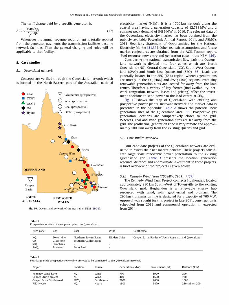
5.1. Queensland network

Concepts are verified through the Queensland network whichis located in the North-Eastern part of the Australian national

Table 2Prospective location of new power plants in Queensland.

NEM zone Gas Coal Wind

NQ Townsville Northern Bowen Basin Flinders

CQ Gladstone Southern Galilee Basin –

SEQ Swanbank – –

SWQ Braemer Surat Basin –

Table 3Four large-scale prospective renewable projects to be connected to the Qu

Project Location Source

Kennedy Wind Farm NQ Wind

Copper String project NQ Wind

Cooper Basin Geothermal SWQ Geothermal

PNG Hydro NQ Hydro

NQ

CQ

SEQ

SWQCooperBasin

NEW SOUTHWALES

SOUTHAUSTRALIA

QUEENSLAND

CoalCCGT

OCGTOilHydro

Wind (prospective)

Coal (prospective)

OCGT (prospective)

Geothermal (prospective)

BulliSouth West Moreton

Wide Bay

GladStone

Central WestNorth

Ross

Far North

Fig. 10. Queensland network of the Australian NEM [29,31].

electricity market (NEM). It is a 1700 km network along thecoastal area having a generation capacity of 12,788 MW and asummer peak demand of 8489 MW in 2010. The relevant data ofthe Queensland electricity market has been obtained from thepublicly available Powerlink Annual Report, 2011, and AEMO’s2011 Electricity Statement of Opportunities for the NationalElectricity Market [31,35]. Other realistic assumptions and futuremarket conjectures are obtained from the ACIL Tasman report,‘Fuel resource, new entry and generation costs in the NEM’ [36].

Considering the national transmission flow path the Queens-land network is divided into four zones which are—NorthQueensland (NQ), Central Queensland (CQ), South West Queens-land (SWQ) and South East Queensland (SEQ) [35]. Loads aregenerally located in the SEQ (63%) region, whereas generationsare mostly in the CQ (48%) and SWQ (40%) regions. Promisingrenewable generation sites are located far away from the loadcentre. Therefore a variety of key factors (fuel availability, net-work congestion, network losses and pricing) affect the invest-ment decisions to send power to the load centre at SEQ.

Fig. 10 shows the map of Queensland with existing andprospective power plants. Relevant network and market data ispresented in the Appendix. Table 2 shows the potential newgeneration sites of the Queensland area [36]. Prospective gasgeneration locations are comparatively closer to the grid.Whereas, coal and wind generation sites are far away from thegrid. The geothermal generation zone is very remote and approxi-mately 1000 km away from the existing Queensland grid.

5.2. Case studies overview

Four candidate projects of the Queensland network are eval-uated to assess their net market benefits. These projects consid-ered large scale renewable power penetration to the existingQueensland grid. Table 3 presents the location, generationresource, distance and approximate investment in these projects.A brief overview of the projects is given below.

5.2.1. Kennedy Wind Farm (700 MW, 290 km) [37]

The Kennedy Wind Farm Project connects Hughenden, locatedapproximately 290 km South-West of Townsville to the existingQueensland grid. Hughenden is a renewable energy hubresourced with wind, solar, geothermal and biomass. The290 km transmission line is designed for a capacity of 700 MW.Approval was sought for this project in late 2011, construction isscheduled from 2012 and commercial operation in expectedfrom 2014.

Geothermal

Shire Cooper Basin, Border of South Australia and Queensland

eensland network.

Generation (MW) Investment (m$) Distance (km)

700 1920 290

400 1680 720

2000 12000 1000

1800 6470 250 cableþ200

K.N. Hasan et al. / Renewable and Sustainable Energy Reviews 18 (2013) 568–582576

5.2.2. Copper String Project (400 MW, 720 km) [38]

The Copper String transmission project connects the Mount Isaregion of North West Queensland to Townsville. It is designed fora capacity of 400 MW with a length of 720 km. This project willprovide opportunities for renewable energy projects surroundingthe proposed transmission line. An environmental impact state-ment (EIS) process is under review for this project. Construction isscheduled to start in late 2012 and the project completion date isearly 2015.

5.2.3. Cooper Basin Geothermal (2000 MW, 1000 km) [39]

The Cooper Basin transmission line connects hot fractured rockbased geothermal power generators located 1000 km away fromthe existing Queensland grid. It is reported that there is apotential of 4000 MW of geothermal power to be connected tothe grid by 2030 [39]. In this case study, transmission connectionis designed for a capacity of 2000 MW. As reported by theGeodynamics, construction and commissioning of a 25 MW com-mercial demonstration plant is scheduled for 2015 [40].

5.2.4. PNG Hydro (1800 MW, 250 km cableþ200 km)

A new transmission line will connect Papua New Guinea (PNG)to the existing NEM grid to provide 1800 MW of hydro power.A 250 km subsea cable along with 200 km overhead transmissionline is designed to transfer baseload hydro power.

As the Queensland network is connected to the other states(i.e., NSW, VIC, SA and TAS) of the NEM, the benefit of thegeneration and transmission expands to the whole NEM network.However, this study only investigates the benefits obtained by theQueensland network.

0100200300400500600700800900

1000

2010 2011 2012 2013 2014

Prod

ucer

Sur

plus

(m$/

year

)

Planning

Copper String Cooper Ba

Fig. 12. Producer surplus of the Queensla

-0.5 0 0.5 1 1.5 2 2.5 3 3.50

1

2

3

4

5

6

7x 10-4

Wind power output data (MW)

Ker

nel d

ensi

ty fu

nctio

n 2001-02, Avg. 1.064MW 2003-04, Avg. 1.278MW 2005-06, Avg. 1.390MW 2007-08, Avg. 1.297MW 2009-10, Avg. 1.243MW 2011-12, Avg. 1.165MW

Fig. 11. Kernel smoothing density estimate of a 3 MW vestas wind turbine output

located in Hughenden (Kennedy wind farm).

5.3. Wind power sensitivity

Historical wind data of last 12 years (2001 to 2012) for CopperString (Hughenden) and Kennedy Wind Farm (Mt. Isa) have beenobtained from the Australian bureau of meteorology [41]. Thosewind data are modelled in MATLAB using the Vestas V112 3 MWwind turbine features (Rated power: 3075 kW, Cut-in wind speed:3 ms�1, Rated wind speed: 12 ms�1, Cut-out wind speed: 25 ms�1,Swept area: 9,852 m2, Frequency: 50/60 Hz) [42]. This type of Vestasturbine is suitable for low and medium wind speed sites, asexperienced in Queensland. The power obtained from the simula-tion is shown as kernel smoothing density estimation as in Fig. 11.

The power obtained from a wind turbine is zero below andnear cut in speed. As the wind speed increases the powerincreases. At 12 ms�1 the power reaches to 3 MW, and until25 ms�1 it gives an output of the same level. Above that speed thewind turbine shuts down. Hence, according to the wind turbinecharacteristics the wind generation have a peak at lower power inkernel density function, and another peak in the rated capacity of3 MW, as shown in Fig. 11.

Capacity factor for the Australian wind farms is usually in therange of 24–45% [43]. This study considers 35% capacity factor ofthese wind farms for all of the calculations. Further, the windpower sensitivity impact on the system performance is discussedin Section 6.8.

6. Analytical results

The impact and potential of future market scenarios areanalysed and ranked based on the net market benefit. Simulationresults are interpreted based on the monetary metrics calculated for arange of market development scenarios. The optimum timing ofintegrating several projects to the Queensland network is analysedfrom simulation results of 2010 to 2020. First, an hourly OPFcalculates the power flows and market dispatch. Then by aggregatingthe producer surplus, consumer surplus, merchandizing surplus,emission tax and LRET benefit underlying these flows/dispatch—thenet market benefit has been obtained. One important point to note isthat the net market benefit presented for every case is calculated bycomparing with the base case scenario.

6.1. Producer surplus

Producer surplus, by using Eq. (10) as obtained from the fourprojects (Copper String, Cooper Basin, Kennedy Wind and PNG

2015 2016 2017 2018 2019 2020Horizon (Year)

sin Kennedy Wind PNG Hydro

nd network for the years 2010–2020.

K.N. Hasan et al. / Renewable and Sustainable Energy Reviews 18 (2013) 568–582 577

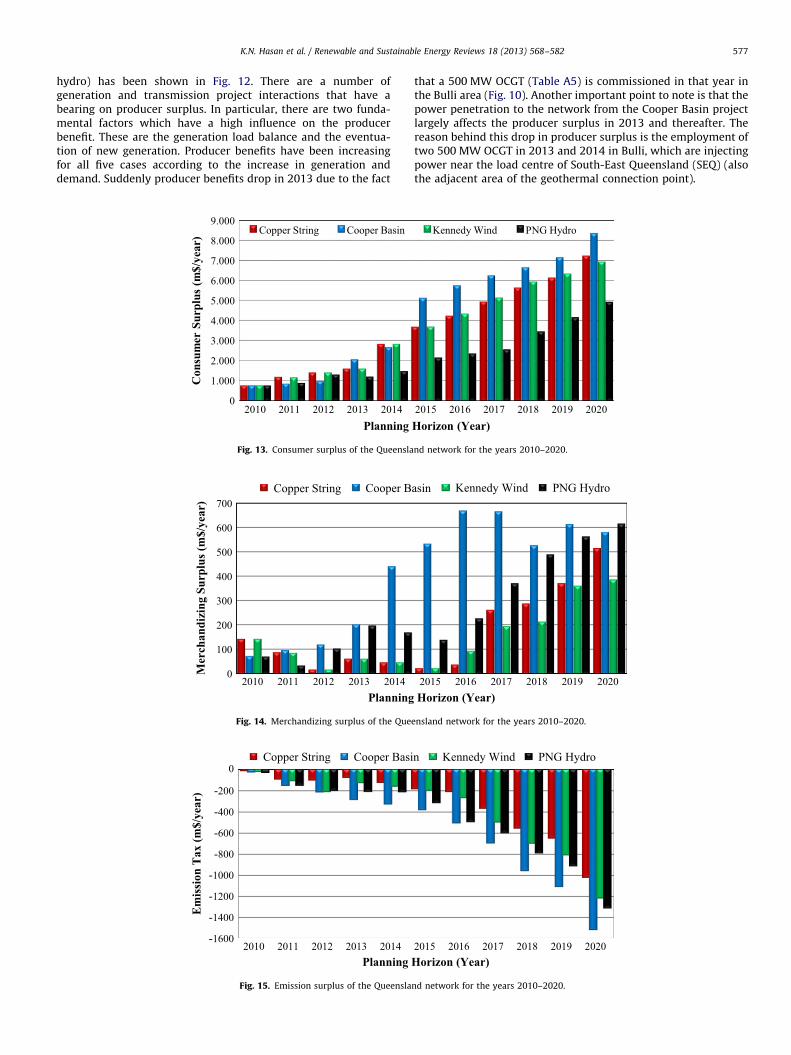
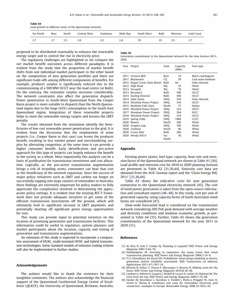
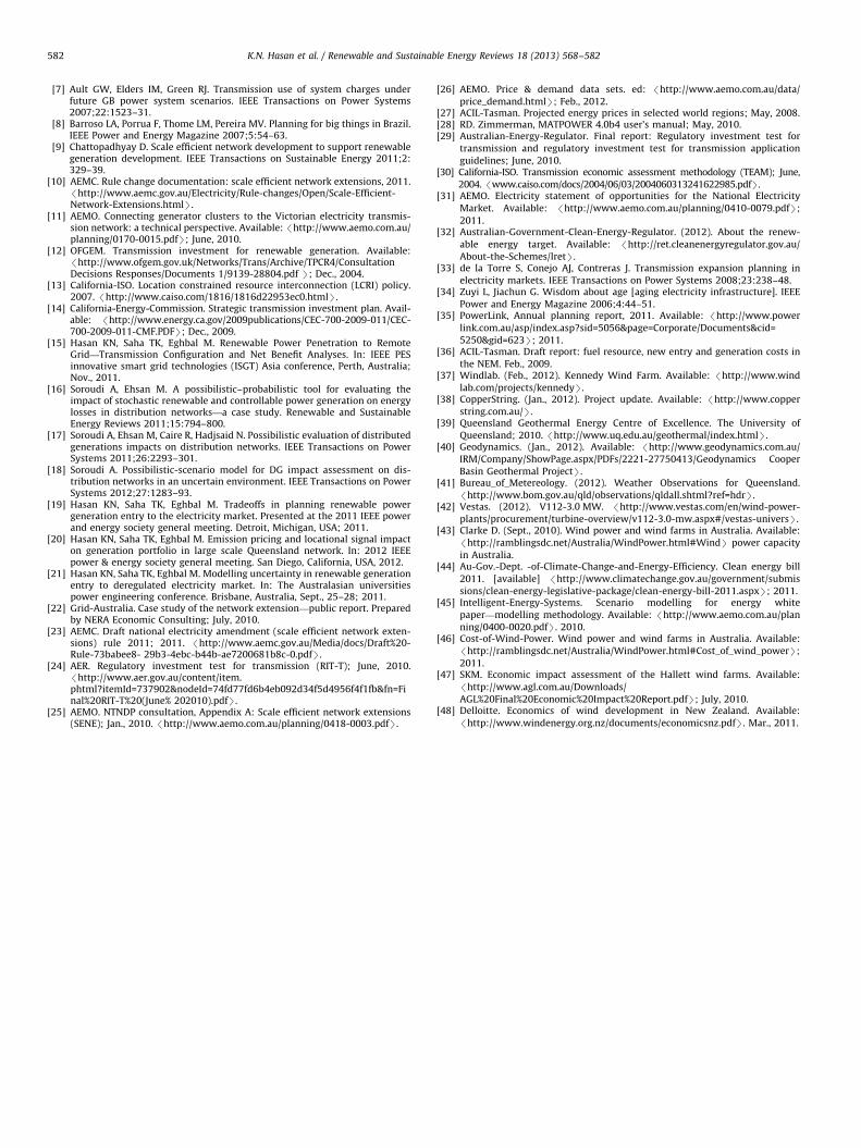
hydro) has been shown in Fig. 12. There are a number ofgeneration and transmission project interactions that have abearing on producer surplus. In particular, there are two funda-mental factors which have a high influence on the producerbenefit. These are the generation load balance and the eventua-tion of new generation. Producer benefits have been increasingfor all five cases according to the increase in generation anddemand. Suddenly producer benefits drop in 2013 due to the fact

0

100

200

300

400

500

600

700

2010 2011 2012 2013 2014

Mer

chan

dizi

ng S

urpl

us (m

$/ye

ar)

Planning

Copper String Cooper B

Fig. 14. Merchandizing surplus of the Que

-1600

-1400

-1200

-1000

-800

-600

-400

-200

0

2010 2011 2012 2013 2014

Em

issi

on T

ax (m

$/ye

ar)

Planning

Copper String Cooper Basi

Fig. 15. Emission surplus of the Queensla

0

1.000

2.000

3.000

4.000

5.000

6.000

7.000

8.000

9.000

2010 2011 2012 2013 2014

Con

sum

er S

urpl

us (m

$/ye

ar)

Planning

Copper String Cooper Basin

Fig. 13. Consumer surplus of the Queensla

that a 500 MW OCGT (Table A5) is commissioned in that year inthe Bulli area (Fig. 10). Another important point to note is that thepower penetration to the network from the Cooper Basin projectlargely affects the producer surplus in 2013 and thereafter. Thereason behind this drop in producer surplus is the employment oftwo 500 MW OCGT in 2013 and 2014 in Bulli, which are injectingpower near the load centre of South-East Queensland (SEQ) (alsothe adjacent area of the geothermal connection point).

2015 2016 2017 2018 2019 2020 Horizon (Year)

asin Kennedy Wind PNG Hydro

ensland network for the years 2010–2020.

2015 2016 2017 2018 2019 2020Horizon (Year)

n Kennedy Wind PNG Hydro

nd network for the years 2010–2020.

2015 2016 2017 2018 2019 2020Horizon (Year)

Kennedy Wind PNG Hydro

nd network for the years 2010–2020.

K.N. Hasan et al. / Renewable and Sustainable Energy Reviews 18 (2013) 568–582578

6.2. Consumer surplus

Fig. 13 shows the consumer surplus as in Eq. (11), for the fourprojects considered in this study. As for producer surplus, con-sumer surplus is affected by the network constraints and genera-tion adequacy. Consumer surpluses are increasing consecutivelyevery year as more consumers are being served with additionalgeneration. The impact of the Cooper basin project is significanton the consumer benefit as it is evident from Fig. 13. The reasonbehind this is the proximity of the point of power injection (Bulli),which is close to the load centre (SEQ) compared to otherprojects. Low cost geothermal power penetration near the loadcentre potentially lessens the LMP, which eventually provides ahigher consumer benefit.

6.3. Merchandizing surplus

Merchandizing surplus, as described in Eq. (12), is calculatedfrom the Copper String, Cooper Basin, Kennedy Wind and PNGhydro projects and have been shown in Fig. 14. As the merchan-dizing surplus represents the difference between the consumerpayment and the producer income it drops off as consumerpayment lessens and vice versa. The yearly incremental merchan-dizing surplus for all of the projects is reasonable due to the loadgrowth and consecutive LMP increment.

6.4. Carbon emission tax

Carbon emission tax imposed on the pollutant power stationsare calculated, by Eq. (13) and presented in Fig. 15. This analysishowever, depends on the carbon price imposed on the emission.The emission payments for specific generators are calculatedbased on the total dispatch, capacity factor, emission factor andthe proposed fixed emission price for the NEM [36,44]. As thedemand is increasing every year the emission taxes paid bythe generators are increasing from 2010 to 2020 for all of the

Table 4LRET benefit of the Queensland network for the years 2010–2020.

Annual LRET 2011 2012 2013 2014

Base case

Required (GW h) [37] 2704 4247 4740 4186

Ren. Gen. (GW h) 2890 3041 3179 3560

Payment (m$) 187 197 206 231

Penalty (m$) [37] 12 78 101 40

0200400600800

10001200140016001800

2011 2012 2013 2014 2015

LR

ET

ben

efit

(m$/

year

)

Planning Ho

Copper String Cooper Basin

Fig. 16. LRET benefit of the Queensland

generators. But comparing with the base case, the carbon emis-sion tax is negative, which means that these renewable powergeneration projects can save the emission tax. It is evident fromFig. 15 that the renewable power penetration to the grid lessensthe amount of emission and consequently the emission tax. Alsothe emission tax depends on the amount of power penetrationand the network constraints to inject renewable power near theload centres. As the point of power penetration of the CooperBasin project is (Bulli) near the load centre (SEQ) compared to theother three projects the renewable power dispatch is higher andthe emission tax is lower compared with the base case.

6.5. LRET payment

The LRET payments for the specified case studies are presentedin Table 4 and in Fig. 16. The required LRET amount is calculatedusing the NEM wide target of the renewable power percentage (asdiscussed in Section 4.1.6) [31,35]. A shortfall of LRET amountimposes a LRET penalty which is A$65/MWh. The LRET incomesfor all of the projects are reported in Fig. 16. As can be seen, theLRET payment is increasing in consecutive years due to thedispatch of more renewable power to the electricity market. LRETbenefit is calculated as the difference in LRET payment for each ofthe four scenarios and that in the base case.

6.6. Net market benefit

Net market benefit and annual revenue requirement (ARR) oncapital for the Copper String, Cooper Basin, Kennedy Wind andPNG hydro projects are shown in Fig. 17. The ARR is calculatedaccording to the discussion of Section 5.2. The main contributionof the net market benefit comes from the consumer benefit,emission tax and LRET payment. The market benefit of CopperString, Cooper Basin, Kennedy Wind Farm and PNG hydro projectovercomes the annual required return on capital from the year2016 and thereafter. Overall the Cooper Basin project offers themaximum net market benefit, followed by the Kennedy Wind

2015 2016 2017 2018 2019 2020

4680 5350 6546 7740 8938 10660

3806 4267 4455 4894 5038 5989

247 277 289 318 327 389

56 70 135 184 253 303

2016 2017 2018 2019 2020rizon (Year)

Kennedy Wind PNG Hydro

network for the years 2010–2020.

K.N. Hasan et al. / Renewable and Sustainable Energy Reviews 18 (2013) 568–582 579

Farm project. Every project in this study is analysed indepen-dently against the base case. Interaction among these projectsmay also give supportive directions for decision making whichwill be addressed in our further research.

-10

-5

0

5

10

15

2010 2011 2012 2013 2014 2015 2016 2017 20

Con

sum

er p

aym

ent (

$/M

Wh)

Planning Horizon (Year)

Fig. 18. Payback scheme of the Queenslan

-35

-15

5

25

45

65

85

Producer Consumer Merchant

Cha

nge

in b

eenf

it w

ith w

ind

(%)

No win

Fig. 19. Changes in market benefit with lower and upper bound the w

-100010003000500070009000

11000130001500017000

2010 2011 2012 2013 2014 2015

Net

Mar

ket B

enef

it (m

$/ye

ar)

Copper String Cooper BasinCopper String Cooper Basin

Fig. 17. Net market benefit and ARR of the Que

6.7. Payback scheme

Three cost recovery mechanisms are considered and theresults are presented in Fig. 18. The ‘total’ scheme (bar charts)

18 2019 2020

Copper String TotalCooper Basin TotalKennedy Wind TotalPNG Hydro TotalCopper String S-2 Cooper Basin S-2 Kennedy Wind S-2 PNG Hydro S-2 Copper String S-1 Cooper Basin S-1Kennedy Wind S-1 PNG Hydro S-1

d network for the years 2010–2020.

Emission LRET Net Benefitd Full wind

ind generation in Copper string and Kennedy wind farm projects.

0

200

400

600

800

1000

1200

1400

2016 2017 2018 2019 2020 Ann

ual R

equi

red

Rev

enue

(m$/

year

)

Kennedy Wind PNG HydroKennedy Wind PNG Hydro

ensland network for the years 2010–2020.

K.N. Hasan et al. / Renewable and Sustainable Energy Reviews 18 (2013) 568–582580

presents the result of the scenario when all cost burdens of thetransmission development are borne by the customers. The ARRon capital is divided by the total generated energy, as presented inEqs. (16) and (17). Schemes S-1 and S-2 divide the total transmis-sion cost among all of the consumers by MWh consumption asdescribed in Section 5.3. Scheme S-1 (solid line) gets the costrecovery from the generators as discussed earlier and presentedin Fig. 9a. Under this scheme, customer payment reduces to zerowith the eventuation of more generators to share the transmis-sion capacity. Scheme S-2 (dashed line) gets back money from thegenerators and pays back a rebate to the customers as discussedearlier and presented in Fig. 9b. Under this scheme, consumersget back money, which is shown by negative payments.

6.8. Wind power sensitivity

While considering the wind power sensitivity in marketanalysis, lower bound (no wind) and upper bound (full wind) ofthe wind power is considered. The impact of these wind power onnet market benefit has been analysed. Consequently, the changesin surpluses of producers, consumers, and merchandisers arecalculated along with the differences in LRET payments andemission pricing.

The impact of wind power intermittency in market simulationhas been shown in Fig. 19. As can be seen from Fig. 19, in no-wind

Table A2Load profile and emission cost mark-up of Queensland electricity market.

2010 2011 2012 2013

Summer peak demand (MW) 8471 9,837 10,241 10,748

Emission cost ($/ton CO2)–ACIL – 23.39 24.19 26.14

Emission cost ($/ton CO2)–AUgovt. – – 23 24.15

Table A1Existing Queensland power plants with fuel-type, capacity, heat-rate and emission

factor.

Name Fuel Capacity (MW) Heat-rate

(GJ/MW h)

Emission factor

(t, CO2/MW h)

Callide B Coal 700 9.97 0.95

Callide C Coal 840 9.47 0.92

Collinsville Coal 187 13.00 1.19

Gladstone Coal 1680 10.23 0.96

Kogan Creek Coal 744 9.60 0.92

Millmerran Coal 852 9.60 0.90

Stanwell Coal 1400 9.89 0.91

SwanbankB Coal 500 11.80 1.09

Tarong Coal 1400 9.94 0.94

Tarong North Coal 443 9.18 0.86

Barcaldine CCGT 36 9.00 0.51

Condamine CCGT 135 7.50 0.40

Darling Downs CCGT 630 7.83 0.42

SwanbankE CCGT 370 7.66 0.43

Townsville CCGT 242 7.83 0.44

Braemer OCGT 504 12.00 0.68

Braemer 2 OCGT 504 12.00 0.68

Oakey OCGT 282 11.04 0.63

Roma OCGT 68 12.00 0.68

Mackay Oil 30 12.86 0.96

MT Stuart Oil 415 12.00 0.90

Yarwun Cogen 160 10.59 0.60

Barron George Hydro 60 – 0

Kareeya Hydro 94 – 0

Wivenhoe Hydro 500 – 0

Windy Hill Wind 12 – 0

Total (MW) 12788 avg. 10.22 avg. 0.65

cases, the consumer surplus, emission benefit and LRET paymentreduces considerably. While the lower ‘short run marginal cost’ ofwind power gives cheaper electricity to consumers, its availabilitymakes a significant difference in consumer surplus. As thepercentage of renewable generation is very less (7%) in Queens-land, the proportion of emission and LRET benefit is high with theavailability/unavailability of full wind capacity. The existingproducers will get more benefit if there is no wind, whereas fullwind generation gives revenue for wind generators though othergenerators will get a lower price due to likely cheaper powerdispatch from wind turbines. Merchandizing surplus changesslightly due to the network utilization by wind generators, butproportionately this is negligible in long Queensland network.

The percentage changes in surpluses of producers [0.7, 0.2]and merchandisers [0.98, 0.8] are not significant compared toconsumers [�7.0, 5.0], emission [�8, 29] and LRET benefit [�30,80]. The net market benefit [�7.0, 6.0] has also been changednoticeably. Net market benefit is the accumulation of all benefitsmentioned above. The scenario of ‘no wind’ to ‘full wind’ changesnet market benefit from �7.0% to 6.0%. As the total market shareof wind capacity in Copper String and Kennedy Wind Farm isaround 11% in the Queensland electricity market, the availabilityand unavailability of wind capacity can largely influence themarket benefits.

7. Conclusions

Although the regulatory framework for transmission invest-ment in a market environment has been an active area ofresearch, there has been little structured effort to date to under-stand the alternative paradigms for encouraging large scalerenewable integration to an existing grid. An analytical frame-work to discuss some of the fundamental challenges associatedwith large scale integration of renewable generation in anelectricity grid is presented in this paper. There are alternativeregulatory paradigms which have their pros and cons that wehave discussed first in the context of different regulatory practicesaround the globe. We have then used a multi-year transmissioninvestment model to assess performance of transmission invest-ment under alternative regulatory paradigms. Four case studiesare presented to enhance remote renewable generation. The netmarket benefit framework is presented accumulating the produ-cer, consumer, merchandiser and environmental surpluses. Theproposed framework captures the long term benefit to obtainmaximum social surplus. Accordingly, the cost allocation is

2014 2015 2016 2017 2018 2019 2020

11,460 12,054 12,633 13,116 13,499 13,836 14,173

28.09 30.04 31.99 33.82 35.43 37.03 38.75

25.40 Market-driven

Table A3Indicative connection costs for new generation entry in the Queensland network.

NEM zone Generation type Transmission cost (m$/MW)

NQ OCGT, CCGT 1.03

CQ OCGT, CCGT 1.43

Geothermal 1.56

SEQ OCGT, CCGT 0.23

SWQ OCGT, CCGT 0.63

Geothermal 1.20

Table A4Load growth in different zones of the Queensland network.

Far North Ross North Central West Gladstone Wide Bay South West Bulli Moreton Gold Coast

2.7 2.7 5.5 3.6 2.2 2.4 19 19 3.5 2.7

Table A5Generation commitment in the Queensland network for the time horizon 2011–

2020.

Year Project Zone Capacity

(MW)

Fuel type

2011 Victoria Mill Ross 19 Black coal/bagasse

2011 Blackwater CQ 30 Coal seam methane

2012 Kogan Creek (Solar Boost) Bulli 44 Solar thermal

2012 High Road NQ 35 Wind

2013 Forsayth NQ 70 Wind

2013 Breamer3 Bulli 500 OCGT

2014 Darling Downs2 Bulli 500 OCGT

2014 Solar Dawn SWQ 250 Solar thermal

2014 Westlink Power Project SWQ 334 OCGT

2015 Burdekin Falls Dam North 37 Hydro

2016 Westlink Power Project SWQ 334 OCGT

2017 Wandoan Power Project SWQ 504 IGCC

2018 Westlink Power Project SWQ 334 OCGT

2019 Spring Gully SWQ 1000 CCGT

2020 Bowen North 200 Wind

2020 Coopers Gap SWQ 350 Wind

2020 Crediton North 90 Wind

2020 Crows Nest Bulli 200 Wind

2020 Windy Hill II Far

North

30 Wind

K.N. Hasan et al. / Renewable and Sustainable Energy Reviews 18 (2013) 568–582 581

proposed to be distributed reasonably to enhance the renewableenergy target and to control the rise in electricity price.

The regulatory challenges are highlighted as we compare thenet market benefit outcomes across different paradigms. It isevident from the study that the proportion of market benefitshifts from one individual market participant to the other basedon the composition of new generation portfolio and there aresignificant trade-offs among different components of benefits. Forexample, producer surplus is significantly reduced due to thecommissioning of a 500 MW OCGT near the load centre (at Bulli).On the contrary, the consumer surplus increases considerably.The network constraints also affect the generation dispatch.Power penetration in South-West Queensland from the CooperBasin project is more suitable to dispatch than the North Queens-land region due to the huge (63%) consumption in the South-EastQueensland region. Integration of these renewable projectshelps to meet the renewable energy targets and lessens the LRETpenalty.

The results obtained from the simulation identify the bene-ficiaries of low cost renewable power penetration to the grid. It isevident from the discussion that the employment of someprojects (i.e., Cooper Basin in this case) can lessen the producerbenefit, resulting in less market power and merchandizing sur-plus by alleviating congestion, at the same time it can provide ahigher consumer benefit. Early identification and pro-activeapproach for this type of projects can largely enhance the benefitto the society as a whole. Most importantly this analysis can be abasis of justification for transmission investment and cost alloca-tion. Logically, as the pro-active transmission augmentationbrings a risk of stranding assets, consumers can bear that costas the beneficiary of the network expansion. Since the success ofmajor policy initiatives such as LRET and carbon tax hinges onsuccessfully tapping into large clusters of renewables in Australia,these findings are extremely important for policy makers to fullyappreciate the complexities involved in determining the appro-priate policy settings. It is evident that the existing RIT-T frame-work does not provide adequate incentive to get some of theefficient transmission investments off the ground, which willultimately lead to significant increase in LRET payments, andpotentially shutting off significant green energy opportunitiesfor ever.

This study can provide input to potential investors on thelocation of promising generation and transmission facilities. Thisinformation could be useful to regulators, system planners andmarket participants about the location, capacity and timing ofgeneration and transmission augmentations.

An extension of this study is expected to incorporate a compara-tive assessment of HVAC, multi-terminal HVDC and hybrid transmis-sion technologies. Some standard models of emission trading schemewill also be implemented in further studies.

Acknowledgements

The authors would like to thank the reviewers for theirinsightful comments. The authors also acknowledge the financialsupport of the Queensland Geothermal Energy Centre of Excel-lence (QGECE), the University of Queensland, Brisbane, Australia.

Appendix

Existing power plants, fuel-type, capacity, heat-rate and emis-sion factor of the Queensland network are shown in Table A1 [36].Load profile and emission cost for 2010 to 2020 planning horizonare presented in Table A2 [31,36,44]. Emission cost data areobtained from the ACIL Tasman report and the ‘Clean Energy Bill,2011’ [31,36,44].

Table A3 shows the indicative costs for new generationconnection to the Queensland electricity network [45]. The costof wind power generation is taken from the open-source informa-tion and consultant reports [46–48]. In this study, cost per unit ofgenerated capacity, using capacity factor of South Australian windfarms are considered [47].

Zone-wide forecasted load is considered on the transmissionnetwork considering 50% PoE peak demand with average weatherand diversity conditions and medium economic growth, as pre-sented in Table A4 [35]. Further, Table A5 shows the generationcommitments of the Queensland network for the year 2011 to2020 [31].

References

[1] de Dios R, Soto F, Conejo AJ. Planning to expand? IEEE Power and EnergyMagazine 2007;5:64–70.

[2] Shahidehpour M. Investing in expansion: the many issues that cloudtransmission planning. IEEE Power and Energy Magazine 2004;2:14–8.

[3] Yi Z, Chowdhury AA, Koval DO. Probabilistic wind energy modeling in electricgeneration system reliability assessment. IEEE Transactions on IndustryApplications 2011;47:1507–14.

[4] Moreno R, Strbac G, Porrua F, Mocarquer S, Bezerra B. Making room for theboom. IEEE Power and Energy Magazine 2010;8:36–46.

[5] Lawhorn J, Osborn D, Caspary J, Nickell B, Larson D, Lasher W, Rahman M. Theview from the top. IEEE Power and Energy Magazine 2009;7:76–88.

[6] Swider DJ, Beurskens L, Davidson S, Twidell J, Pyrko J, Pruggler W, Auer H,Vertin K, Skema R. Conditions and costs for renewables electricity gridconnection: examples in Europe. Renewable Energy 2008;33:1832–42.

K.N. Hasan et al. / Renewable and Sustainable Energy Reviews 18 (2013) 568–582582

[7] Ault GW, Elders IM, Green RJ. Transmission use of system charges underfuture GB power system scenarios. IEEE Transactions on Power Systems2007;22:1523–31.

[8] Barroso LA, Porrua F, Thome LM, Pereira MV. Planning for big things in Brazil.IEEE Power and Energy Magazine 2007;5:54–63.

[9] Chattopadhyay D. Scale efficient network development to support renewablegeneration development. IEEE Transactions on Sustainable Energy 2011;2:329–39.

[10] AEMC. Rule change documentation: scale efficient network extensions, 2011./http://www.aemc.gov.au/Electricity/Rule-changes/Open/Scale-Efficient-Network-Extensions.htmlS.

[11] AEMO. Connecting generator clusters to the Victorian electricity transmis-sion network: a technical perspective. Available: /http://www.aemo.com.au/planning/0170-0015.pdfS; June, 2010.

[12] OFGEM. Transmission investment for renewable generation. Available:/http://www.ofgem.gov.uk/Networks/Trans/Archive/TPCR4/ConsultationDecisions Responses/Documents 1/9139-28804.pdf S; Dec., 2004.

[13] California-ISO. Location constrained resource interconnection (LCRI) policy.2007. /http://www.caiso.com/1816/1816d22953ec0.htmlS.

[14] California-Energy-Commission. Strategic transmission investment plan. Avail-able: /http://www.energy.ca.gov/2009publications/CEC-700-2009-011/CEC-700-2009-011-CMF.PDFS; Dec., 2009.

[15] Hasan KN, Saha TK, Eghbal M. Renewable Power Penetration to RemoteGrid—Transmission Configuration and Net Benefit Analyses. In: IEEE PESinnovative smart grid technologies (ISGT) Asia conference, Perth, Australia;Nov., 2011.

[16] Soroudi A, Ehsan M. A possibilistic–probabilistic tool for evaluating theimpact of stochastic renewable and controllable power generation on energylosses in distribution networks—a case study. Renewable and SustainableEnergy Reviews 2011;15:794–800.

[17] Soroudi A, Ehsan M, Caire R, Hadjsaid N. Possibilistic evaluation of distributedgenerations impacts on distribution networks. IEEE Transactions on PowerSystems 2011;26:2293–301.

[18] Soroudi A. Possibilistic-scenario model for DG impact assessment on dis-tribution networks in an uncertain environment. IEEE Transactions on PowerSystems 2012;27:1283–93.

[19] Hasan KN, Saha TK, Eghbal M. Tradeoffs in planning renewable powergeneration entry to the electricity market. Presented at the 2011 IEEE powerand energy society general meeting. Detroit, Michigan, USA; 2011.

[20] Hasan KN, Saha TK, Eghbal M. Emission pricing and locational signal impacton generation portfolio in large scale Queensland network. In: 2012 IEEEpower & energy society general meeting. San Diego, California, USA, 2012.

[21] Hasan KN, Saha TK, Eghbal M. Modelling uncertainty in renewable generationentry to deregulated electricity market. In: The Australasian universitiespower engineering conference. Brisbane, Australia, Sept., 25–28; 2011.

[22] Grid-Australia. Case study of the network extension—public report. Preparedby NERA Economic Consulting; July, 2010.

[23] AEMC. Draft national electricity amendment (scale efficient network exten-sions) rule 2011; 2011. /http://www.aemc.gov.au/Media/docs/Draft%20-Rule-73babee8- 29b3-4ebc-b44b-ae7200681b8c-0.pdfS.

[24] AER. Regulatory investment test for transmission (RIT-T); June, 2010./http://www.aer.gov.au/content/item.phtml?itemId=737902&nodeId=74fd77fd6b4eb092d34f5d4956f4f1fb&fn=Final%20RIT-T%20(June% 202010).pdfS.

[25] AEMO. NTNDP consultation, Appendix A: Scale efficient network extensions(SENE); Jan., 2010. /http://www.aemo.com.au/planning/0418-0003.pdfS.

[26] AEMO. Price & demand data sets. ed: /http://www.aemo.com.au/data/price_demand.htmlS; Feb., 2012.

[27] ACIL-Tasman. Projected energy prices in selected world regions; May, 2008.[28] RD. Zimmerman, MATPOWER 4.0b4 user’s manual; May, 2010.[29] Australian-Energy-Regulator. Final report: Regulatory investment test for

transmission and regulatory investment test for transmission applicationguidelines; June, 2010.

[30] California-ISO. Transmission economic assessment methodology (TEAM); June,2004. /www.caiso.com/docs/2004/06/03/2004060313241622985.pdfS.

[31] AEMO. Electricity statement of opportunities for the National ElectricityMarket. Available: /http://www.aemo.com.au/planning/0410-0079.pdfS;

2011.[32] Australian-Government-Clean-Energy-Regulator. (2012). About the renew-

able energy target. Available: /http://ret.cleanenergyregulator.gov.au/About-the-Schemes/lretS.

[33] de la Torre S, Conejo AJ, Contreras J. Transmission expansion planning inelectricity markets. IEEE Transactions on Power Systems 2008;23:238–48.

[34] Zuyi L, Jiachun G. Wisdom about age [aging electricity infrastructure]. IEEEPower and Energy Magazine 2006;4:44–51.

[35] PowerLink, Annual planning report, 2011. Available: /http://www.power

link.com.au/asp/index.asp?sid=5056&page=Corporate/Documents&cid=5250&gid=623S; 2011.

[36] ACIL-Tasman. Draft report: fuel resource, new entry and generation costs inthe NEM. Feb., 2009.

[37] Windlab. (Feb., 2012). Kennedy Wind Farm. Available: /http://www.windlab.com/projects/kennedyS.

[38] CopperString. (Jan., 2012). Project update. Available: /http://www.copperstring.com.au/S.

[39] Queensland Geothermal Energy Centre of Excellence. The University ofQueensland; 2010. /http://www.uq.edu.au/geothermal/index.htmlS.

[40] Geodynamics. (Jan., 2012). Available: /http://www.geodynamics.com.au/IRM/Company/ShowPage.aspx/PDFs/2221-27750413/Geodynamics CooperBasin Geothermal ProjectS.

[41] Bureau_of_Metereology. (2012). Weather Observations for Queensland./http://www.bom.gov.au/qld/observations/qldall.shtml?ref=hdrS.

[42] Vestas. (2012). V112-3.0 MW. /http://www.vestas.com/en/wind-power-plants/procurement/turbine-overview/v112-3.0-mw.aspx#/vestas-universS.

[43] Clarke D. (Sept., 2010). Wind power and wind farms in Australia. Available:/http://ramblingsdc.net/Australia/WindPower.html#WindS power capacity

in Australia.[44] Au-Gov.-Dept. -of-Climate-Change-and-Energy-Efficiency. Clean energy bill

2011. [available] /http://www.climatechange.gov.au/government/submissions/clean-energy-legislative-package/clean-energy-bill-2011.aspxS; 2011.

[45] Intelligent-Energy-Systems. Scenario modelling for energy whitepaper—modelling methodology. Available: /http://www.aemo.com.au/planning/0400-0020.pdfS. 2010.

[46] Cost-of-Wind-Power. Wind power and wind farms in Australia. Available:/http://ramblingsdc.net/Australia/WindPower.html#Cost_of_wind_powerS;

2011.[47] SKM. Economic impact assessment of the Hallett wind farms. Available:

/http://www.agl.com.au/Downloads/AGL%20Final%20Economic%20Impact%20Report.pdfS; July, 2010.

[48] Delloitte. Economics of wind development in New Zealand. Available:

/http://www.windenergy.org.nz/documents/economicsnz.pdfS. Mar., 2011.