Renewable and Sustainable Energy Reviews 25 (2013) 494–502

Contents lists available at SciVerse ScienceDirect

Renewable and Sustainable Energy Reviews

1364-03http://d

n CorrE-m

ilhanoztchanam

1 Te

journal homepage: www.elsevier.com/locate/rser

Revisiting the environmental Kuznets curve in a global economy

Muhammad Shahbaz a,n, Ilhan Ozturk b,1, Talat Afza c, Amjad Ali d

a Department of Management Sciences, COMSATS Institute of Information Technology, Lahore, Pakistanb Faculty of Economics and Administrative Sciences, Cag University, 33800 Mersin, Turkeyc COMSATS Institute of Information Technology, Defence Road, Off Raiwind, Lahore, Pakistand School of Social Sciences, National College of Business Administration & Economics, 40/E-1, Gulberg III, Lahore 54660, Pakistan

a r t i c l e i n f o

Article history:Received 11 March 2013Received in revised form28 April 2013Accepted 7 May 2013Available online 5 June 2013

Keywords:Carbon dioxide emissionsEconomic growth

21/$ - see front matter & 2013 Elsevier Ltd. Ax.doi.org/10.1016/j.rser.2013.05.021

esponding author.ail addresses: shahbazmohd@live.com (M. Shaurk@cag.edu.tr (I. Ozturk), talatafza@ciitlahorjadali@yahoo.com (A. Ali).l./fax: +90 324 6514828.

a b s t r a c t

The present study deals with an empirical investigation between CO2 emissions, energy intensity,economic growth and globalization using annual data over the period of 1970–2010 for Turkish economy.We applied unit root test and cointegration approach in the presence of structural breaks. The directionof causality between the variables is investigated by applying the VECM Granger causality approach. Ourresults confirmed the existence of cointegration between the series. The empirical evidence reported thatenergy intensity and economic growth (globalization) increase (condense) CO2 emissions. The resultsalso validated the presence of environmental Kuznets curve (EKC). The causality analysis showsbidirectional causality between economic growth and CO2 emissions. This implies that economic growthcan be boosted at the cost of environment.

& 2013 Elsevier Ltd. All rights reserved.

Contents

1. Introduction . . . . . . . . . . . . . . . . . . . . . . . . . . . . . . . . . . . . . . . . . . . . . . . . . . . . . . . . . . . . . . . . . . . . . . . . . . . . . . . . . . . . . . . . . . . . . . . . . . . . . . . . 4942. Literature review . . . . . . . . . . . . . . . . . . . . . . . . . . . . . . . . . . . . . . . . . . . . . . . . . . . . . . . . . . . . . . . . . . . . . . . . . . . . . . . . . . . . . . . . . . . . . . . . . . . . 4953. The data, modeling and estimation strategy . . . . . . . . . . . . . . . . . . . . . . . . . . . . . . . . . . . . . . . . . . . . . . . . . . . . . . . . . . . . . . . . . . . . . . . . . . . . . . 496

3.1. The data and modeling . . . . . . . . . . . . . . . . . . . . . . . . . . . . . . . . . . . . . . . . . . . . . . . . . . . . . . . . . . . . . . . . . . . . . . . . . . . . . . . . . . . . . . . . . 4963.2. Zivot–Andrews unit root test . . . . . . . . . . . . . . . . . . . . . . . . . . . . . . . . . . . . . . . . . . . . . . . . . . . . . . . . . . . . . . . . . . . . . . . . . . . . . . . . . . . . 4973.3. The ARDL cointegration. . . . . . . . . . . . . . . . . . . . . . . . . . . . . . . . . . . . . . . . . . . . . . . . . . . . . . . . . . . . . . . . . . . . . . . . . . . . . . . . . . . . . . . . . 4973.4. The VECM Granger causality . . . . . . . . . . . . . . . . . . . . . . . . . . . . . . . . . . . . . . . . . . . . . . . . . . . . . . . . . . . . . . . . . . . . . . . . . . . . . . . . . . . . . 498

4. Results discussion . . . . . . . . . . . . . . . . . . . . . . . . . . . . . . . . . . . . . . . . . . . . . . . . . . . . . . . . . . . . . . . . . . . . . . . . . . . . . . . . . . . . . . . . . . . . . . . . . . . 4985. Conclusion and policy implications . . . . . . . . . . . . . . . . . . . . . . . . . . . . . . . . . . . . . . . . . . . . . . . . . . . . . . . . . . . . . . . . . . . . . . . . . . . . . . . . . . . . . 501References . . . . . . . . . . . . . . . . . . . . . . . . . . . . . . . . . . . . . . . . . . . . . . . . . . . . . . . . . . . . . . . . . . . . . . . . . . . . . . . . . . . . . . . . . . . . . . . . . . . . . . . . . . . . . 501

1. Introduction

Turkey has experienced a significant rise in economic growth,energy consumption and carbon emissions during the last twodecades. Turkey is a candidate for full membership of EuropeanUnion (EU) and therefore is likely to face significant pressures fromEU during negotiations to introduce its national plan on climatechange and global warming along with specific emissions targets [1].Turkey is one of the important countries which have a high carbon

ll rights reserved.

hbaz),e.edu.pk (T. Afza),

emissions and economic growth in the world. The reports of WorldBank and UNDP indicate that CO2 emissions would rise more thansix-fold by the end of 2025 rather than 1990s, so it is a greatchallenge for Turkey to achieve both the targets of high economicgrowth and less CO2 emissions at the same time.

The present study contributes in energy economics by fourways: (i), we augmented the CO2 emissions function by incorpor-ating globalization as a potential determinant of energy intensity,economic growth and CO2 emissions; (ii) Zivot–Andrews [2] unitroot test has been applied in determining integrating order of thevariables; (iii) Gregory–Hansen structural break cointegration testis used to examine the robustness of long run relationshipbetween the variables; and (iv) direction of causal relation isinvestigated by applying the VECM Granger causality test. Ourfindings confirm the existence of long run relationship between

M. Shahbaz et al. / Renewable and Sustainable Energy Reviews 25 (2013) 494–502 495

economic growth, energy intensity, globalization and CO2 emis-sions. We find that the EKC is validated in case of Turkey. More-over, energy intensity is a, major contributor to CO2 emissions, andglobalization improves the environmental quality. The feedbackeffect exists between economic growth and CO2 emissions. Energyintensity and globalization Granger cause CO2 emissions.

The rest of the paper is organized as follows: Section 2 presentsreview of literature; Section 3 provides data information, model-ing and estimation strategy; result interpretations are in Section 4and Section 5 deals with conclusion and policy implications.

2. Literature review

In 1991, Grossman and Krueger started the debate of environ-mental Kuznets curve (EKC) which explained the relationshipbetween environmental pollution and economic growth i.e.inverted U-shaped relationship. Later on, a series of debate hasstarted by investigating the relationship between environmentalpollution and economic development. Johansson and Kriström [3]noted that the literature on EKC is not enough and this topic needsmore empirical investigation. But Stern [4] argued the issues ofEKC should be revisited by using new models and new decom-positions with different panels and time series data sets. Similarly,Wagner [5] pointed out that the data on per capita CO2 emissionsand per capita GDP are not stationary in time series frameworkand this problem is not sufficiently addressed in literature. There-fore, many dimensions of EKC are available for further empiricalinvestigation.

Existing literature provides two strands of relationshipbetween energy consumption and energy emissions i.e. economicgrowth and energy consumption and, economic growth and CO2

emissions in case of Turkey (see [6], for literature survey onenergy-growth nexus). For example, Altinaya and Karagol [7]investigated the direction of causality between energy consump-tion and economic growth. They applied unit root test to examinestationarity properties of the variables. The Hsiao Granger caus-ality was applied using time series data over the period 1950–2000. Their empirical exercise reported the neutral effect betweeneconomic growth and energy consumption. Lise and Montfort [8]probed the relationship between gross domestic product andenergy consumption using annual data for the period of 1970–2003. The Granger causality analysis found unidirectional causalityrunning from economic growth to energy consumption.

Soytas and Sari [9] analyzed the relationship between energyconsumption in industrial and manufacturing sectors using multi-variate model by incorporating capital and labor in production

Table 1Summary of studies on Turkey.

No. Authors Time period Variables

1. Altinaya and Karagol [7] 1950–2000 GDP per capita, energy cons2. Lisea [19] 1980–2003 GNP growth, CO2 emissions3. Lise and Montfort [8] 1970–2003 GDP per capita, energy cons4. Soytas and Sari [9] 1968–2002 Energy consumption, indust5. Jober and Karanfil [10] 1960–2003 GNP growth, energy consum6. Erdal et al. [11] 1970–2006 Energy consumption, GNP p7. Akbostanci et al. [13] 1992–2001, GDP per capita, CO2 emissio

1968–20038. Halicioglu [14] 1960–2005 Income, CO2 emissions, ener9. Soytas and Sari [15] 1960–2000 GNP, CO2 emission, energy c10. Ozturk and Acaravci [1] 1968–2005 GNP per capita, CO2 emissio11. Jobert et al. [17] 1970–2008 GNP per capita, CO2emission12. Kaplan et al. [12] 1971–2006 GNP per capita, energy cons13. Joberta and Karanfil [18] 1971–2008 Energy consumption, CO2 em14. Ozturk et al. [20] 1960–2006 GNP growth, energy consum

function. Their results indicated cointegration between the vari-ables for long run relationship. The results of vector error correc-tion (VECM) model reveal that there is unidirectional causalityrunning from energy consumption to manufacturing GDP. Further-more, the results of variance decomposition and generalizedimpulse response analysis confirmed that energy consumption isan important factor of manufacturing GDP. This implies thatutilization of energy saving modes and energy efficiency technol-ogy may enhance manufacturing production in Turkey. Similarly,Jober and Karanfil [10] reinvestigated the relationship betweenenergy consumption and economic growth at aggregate level andat sectoral industry level. Their results reported that there is nocausality between both variables at aggregate level as well assectoral level.

Erdal et al. [11] used the data over the period of 1970–2006 toreexamine the relationship between energy consumption and realGNP. They applied augmented Dickey–Fuller (ADF) and Philips–Perron (PP) unit root tests to test stationarity properties of bothvariables and Johansen cointegration for long run as well as Grangercausality test for pair-wise causality. The empirical exercise reportedthe cointegration between energy consumption and real GNP. Thecausality analysis revealed feedback effect implying that economicgrowth and energy consumption are interdependent. This suggeststhat any negative energy shock will put negative effect on economicgrowth of Turkey. Kaplan et al. [12] reexamined the causal relation-ship between economic growth and energy consumption over theperiod 1971–2006 using supply and demand side models. Theirresults found long run relationship as cointegration is found betweenthe series. The causality analysis found feedback effect betweeneconomic growth and energy consumption. This shows that forachieving high level of economic growth more energy is neededand supply of energy further enhances economic growth, implyingthat any shock which occurred in supply of energy puts a negativeimpact on economic growth.

The second strand deals with the relationship between eco-nomic growth and CO2 emissions such as, Akbostanci et al. [13]tested the direction of causality between income and environ-mental degradation using various stages of economic developmentusing PM10 and SO2 measures of environmental degradation. Theyused data of 58 provinces of Turkey over the period 1968–2003.Their empirical results unveiled that CO2 emissions and incomehave long run relationship but inverted U-shaped relationship isfound when they SO2 and PM10 are used as measures of environ-mental degradation. The results do not support EKC hypothesisbased on income and environmental degradation nexus.

Halicioglu [14] augmented CO2 emissions function by incorpor-ating trade to investigate the causal relationship between income,

Cointegration EKC hypothesis

umption – –

– –

umption Yes –

rial value-added Yes –

ption – –

er capita Yes –

ns Yes EKC does not exist

gy consumption, trade openness Yes –

onsumption Yes –

ns, energy consumption, employment Yes EKC does not exists, energy consumption – EKC existsumption Yes –

issions, real GDP per capita – EKC existsption Yes –

2 See in details http://globalization.kof.ethz.ch/.

M. Shahbaz et al. / Renewable and Sustainable Energy Reviews 25 (2013) 494–502496

CO2 emissions and energy consumption for the period 1960–2005.Halicioglu found cointegration by applying the ARDL boundstesting approach to cointegration. The results showed that GDPis highly significant among other variables of the model inexplaining CO2 emissions in case of Turkey. Soytas and Sari [15]reexamined the relationship between economic growth, CO2

emissions and energy by incorporating capital formation and laboras potential determinants of economic growth and CO2 emissions.Their results exposed that CO2 emissions Granger cause energyconsumption but same and vice versa which implies that byreducing CO2 emissions, Turkey may not forgo economic growth.Kaygusuz [16] investigated the electricity and energy demandfunctions and their empirical exercise found that rapid energyconsumption and energy production are linked with environmen-tal issues at national level as a rise in energy consumption(electricity consumption) increases CO2 emissions.

Ozturk and Acaravci [1] reinvestigated the cointegration andcausality between economic growth, CO2 emissions and energyconsumption by incorporating employment using time series dataover the period 1968–2005. Their results indicated the existence ofcointegration between the variables and found that incomeelasticity of CO2 emissions is inelastic (−0.606) but incomeelasticity of energy consumptions is more elastic (1.375). Theiranalysis could not provide the empirical validation of the EKChypothesis. The causality analysis found neutral effect betweenenergy consumption and economic growth, economic growth andCO2 emissions and, energy consumption and CO2 emissions. Thisimplies that the adoption of energy conservation has no adverseeffect on growth rate of real GDP. Jobert et al. [17] probed therelationship between economic growth, CO2 emissions and energyconsumption by applying Bayesian empirical model. The studyused time series data of 50 countries including Turkey over theperiod of 1970–2008. Their empirical analysis reported thatexistence of the EKC is sensitive with respect to countries butEKC exists in case of Turkey. Joberta and Karanfil [18] used cross-country data including Turkey to test the validation of EKC andfound the existence of EKC before 1980. The threshold level ofincome is rising which was reported as 10,000 in early 1980 and20,000 in 2008 (Table 1).

The 21st century has increased the internationalization amongthe world economies and countries are more closely linked witheach other economically, politically and culturally. Globalizationwhich is based on economics facilitates and helps in the promo-tion of division of labor and increases the comparative advantageof different nations. Globalization improves the total factor pro-ductivity by increasing trade activity but also boosts economicactivity via foreign direct investment and transfer of advancedtechnology from developed countries to developing nations.Globalization also provides investment opportunities includingforeign direct investment and develops the financial markets.Globalization directly enhances trade and then economic growthwhile indirectly, it promotes investment opportunities not only inthe form of domestic investment but also in foreign investment,which not only influences energy demand but also influences theenvironment.

Various researchers have used different measures of globaliza-tion to examine its impact on environmental degradation. Forinstance, Grossman and Krueger [21] investigated the environ-mental impact of Northern America Free Trade Agreement(NAFTA) on environment. They reported that trade openness(globalization) affects environmental degradation via scale effectkeeping composition effect and technique effect constant. Simi-larly, Dinda [22] claimed that environmental degradation increasesas scale effect dominates the composition effect and techniqueeffect and same conclusion is drawn by Shahbaz et al. [23] thattrade openness declines CO2 emissions in case of Pakistan. On the

contrary, Wheeler [24] noted that globalization reduces environ-mental degradation due to the investment in energy-efficienttechnologies for production. Copeland and Taylor [25] reportedthat globalization facilitates transfer pollution intensive technol-ogy to countries where environmental regulation are weak (indeveloping economies). In such circumstances, developed coun-tries attain benefits from trade openness at the cost of environ-ment in developing economies. Copeland and Taylor [26] pointedthat trade depends upon the relative abundance of factor endow-ment in each country and therefore, comparative advantage oftrade also affects environmental quality depending upon trade andenvironmental policy in the country. Birdsall and Wheeler [27],Lee and Roland-Host, [28], Jones and Rodolfo [29] opined thatenvironmental degradation is not the main cause of trade open-ness. Similarly, Antweiler et al. [30] and Liddle [31] pointed outthat trade openness improves environmental quality via techniqueeffect. Environmental regulations become strict as incomeincreases and the adoption of energy-efficient technologies areencouraged to save environment from degradation. In case ofChina, Dean [32] reported that trade openness deteriorates envir-onmental quality via improved terms of trade, however, rise inincome saves environment from degradation. Magani [33] useddata of 63 developed and developing economies to examine theeffect of trade openness on energy emissions. The results showedthat a 0.58% carbon emission is linked with a 1% increase in trade.Similarly, McAusland [34] reported that trade affects environmentsignificantly and same view is confirmed by Frankel [35].

3. The data, modeling and estimation strategy

3.1. The data and modeling

We have used data of energy intensity per capita, CO2 emis-sions per capita, real GDP per capita and globalization index toprobe the existence of environmental Kuznets curve (EKC) in caseof Turkey. The data on energy consumption (kilotons of oilequivalent), CO2 emissions (metric tons) and real GDP (Turkishcurrency) has been attained from world development indicators(CD-OM, 2012). The series population is used to convert all seriesinto per capita. The data on KOF globalization index is borrowedfrom Dreher [36]. The globalization index is constructed fromthree sub-indices (social, economic and political globalization).2

The study covers the period of 1970–2010. The general functionalform of our model is given in the as following equation:

ΔCt ¼ f ðEt ; Yt ; Y2t ; GtÞ ð1Þ

We have transformed all the variables into natural logarithmfollowing Shahbaz et al. [23,37]. The empirical form of our modelis constructed as follows:

lnCt ¼ α1 þ αElnEt þ αY lnYt þ αY2 lnY2t þ αGlnGt þ μt ð2Þ

where lnCt is natural log of CO2 emissions per capita, natural logenergy intensity per capita is indicated by lnEt , lnYt (lnY2

t ) is thenatural log of real GDP per capita (square of real GDP per capita)and lnGt is for natural log of KOF index of globalization. μt is theerror term assumed to be having normal distribution with zeromean and predictable variance. We expect that impact of energyconsumption on CO2 emissions and αE40. The relationshipbetween economic growth and CO2 emissions inverted U-shapedif αY 40 and αY2 o0 otherwise U-shaped if αY o0 and αY2 40.αGo0 if energy-efficient technology via foreign direct investmentand trade is encouraged for domestic production otherwise αG40.

M. Shahbaz et al. / Renewable and Sustainable Energy Reviews 25 (2013) 494–502 497

3.2. Zivot–Andrews unit root test

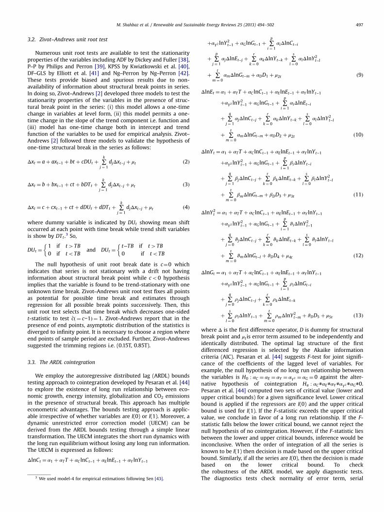
Numerous unit root tests are available to test the stationarityproperties of the variables including ADF by Dickey and Fuller [38],P–P by Philips and Perron [39], KPSS by Kwiatkowski et al. [40],DF–GLS by Elliott et al. [41] and Ng–Perron by Ng–Perron [42].These tests provide biased and spurious results due to non-availability of information about structural break points in series.In doing so, Zivot–Andrews [2] developed three models to test thestationarity properties of the variables in the presence of struc-tural break point in the series: (i) this model allows a one-timechange in variables at level form, (ii) this model permits a one-time change in the slope of the trend component i.e. function and(iii) model has one-time change both in intercept and trendfunction of the variables to be used for empirical analysis. Zivot–Andrews [2] followed three models to validate the hypothesis ofone-time structural break in the series as follows:

Δxt ¼ aþ axt−1 þ bt þ cDUt þ ∑k

j ¼ 1djΔxt−j þ μt ð2Þ

Δxt ¼ bþ bxt−1 þ ct þ bDTt þ ∑k

j ¼ 1djΔxt−j þ μt ð3Þ

Δxt ¼ cþ cxt−1 þ ct þ dDUt þ dDTt þ ∑k

j ¼ 1djΔxt−j þ μt ð4Þ

where dummy variable is indicated by DUt showing mean shiftoccurred at each point with time break while trend shift variablesis show by DTt .3 So,

DUt ¼1 if t4TB

0 if toTBand DUt ¼

t−TB if t4TB

0 if toTB

��

The null hypothesis of unit root break date is c¼0 whichindicates that series is not stationary with a drift not havinginformation about structural break point while co0 hypothesisimplies that the variable is found to be trend-stationary with oneunknown time break. Zivot–Andrews unit root test fixes all pointsas potential for possible time break and estimates throughregression for all possible break points successively. Then, thisunit root test selects that time break which decreases one-sidedt-statistic to test cð ¼ c−1Þ ¼ 1. Zivot–Andrews report that in thepresence of end points, asymptotic distribution of the statistics isdiverged to infinity point. It is necessary to choose a region whereend points of sample period are excluded. Further, Zivot–Andrewssuggested the trimming regions i.e. (0.15T, 0.85T).

3.3. The ARDL cointegration

We employ the autoregressive distributed lag (ARDL) boundstesting approach to cointegration developed by Pesaran et al. [44]to explore the existence of long run relationship between eco-nomic growth, energy intensity, globalization and CO2 emissionsin the presence of structural break. This approach has multipleeconometric advantages. The bounds testing approach is applic-able irrespective of whether variables are I(0) or I(1). Moreover, adynamic unrestricted error correction model (UECM) can bederived from the ARDL bounds testing through a simple lineartransformation. The UECM integrates the short run dynamics withthe long run equilibrium without losing any long run information.The UECM is expressed as follows:

ΔlnCt ¼ α1 þ αTT þ αC lnCt−1 þ αElnEt−1 þ αY lnYt−1

3 We used model-4 for empirical estimations following Sen [43].

þαY2 lnY2t−1 þ αGlnGt−1 þ ∑

p

i ¼ 1αiΔlnCt−i

þ ∑p

j ¼ 1αjΔlnEt−j þ ∑

r

k ¼ 0αkΔlnYt−k þ ∑

s

l ¼ 0αlΔlnY

2t−l

þ ∑t

m ¼ 0αmΔlnGt−m þ αDD1 þ μ2t ð9Þ

ΔlnEt ¼ α1 þ αTT þ αC lnCt−1 þ αElnEt−1 þ αY lnYt−1

þαY2 lnY2t−1 þ αGlnGt−1 þ ∑

p

i ¼ 1αiΔlnEt−i

þ ∑q

j ¼ 1αjΔlnCt−j þ ∑

r

k ¼ 0αkΔlnYt−k þ ∑

s

l ¼ 0αlΔlnY

2t−l

þ ∑t

m ¼ 0αmΔlnGt−m þ αDD2 þ μ2t ð10Þ

ΔlnYt ¼ α1 þ αTT þ αC lnCt−1 þ αElnEt−1 þ αY lnYt−1

þαY2 lnY2t−1 þ αGlnGt−1 þ ∑

p

i ¼ 1βiΔlnYt−i

þ ∑q

j ¼ 1βjΔlnCt−j þ ∑

r

k ¼ 0βkΔlnEt−k þ ∑

s

l ¼ 0βlΔlnY

2t−l

þ ∑t

m ¼ 0βmΔlnGt−m þ βDD3 þ μ3t ð11Þ

ΔlnY2t ¼ α1 þ αTT þ αC lnCt−1 þ αElnEt−1 þ αY lnYt−1

þαY2 lnY2t−1 þ αGlnGt−1 þ ∑

p

i ¼ 1ϑiΔlnY

2t−1

þ ∑q

j ¼ 0ϑjΔlnCt−j þ ∑

r

k ¼ 0ϑkΔlnEt−k þ ∑

s

l ¼ 0ϑlΔlnYt−l

þ ∑t

m ¼ 0ϑmΔlnGt−l þ ϑDD4 þ μ4t ð12Þ

ΔlnGt ¼ α1 þ αTT þ αC lnCt−1 þ αElnEt−1 þ αY lnYt−1

þαY2 lnY2t−1 þ αGlnGt−1 þ ∑

p

i ¼ 1ρiΔlnGt−i

þ ∑q

j ¼ 0ρjΔlnCt−j þ ∑

r

k ¼ 0ρkΔlnEt−k

þ ∑s

l ¼ 0ρlΔlnYt−1 þ ∑

t

m ¼ 0ρmΔlnY

2t−m þ ϑDD5 þ μ5t ð13Þ

where Δ is the first difference operator, D is dummy for structuralbreak point and μt is error term assumed to be independently andidentically distributed. The optimal lag structure of the firstdifferenced regression is selected by the Akaike informationcriteria (AIC). Pesaran et al. [44] suggests F-test for joint signifi-cance of the coefficients of the lagged level of variables. Forexample, the null hypothesis of no long run relationship betweenthe variables is H0 : αC ¼ αE ¼ αY ¼ αY2 ¼ αG ¼ 0 against the alter-native hypothesis of cointegration Ha : αC≠αE≠αY≠αY2≠αG≠0.Pesaran et al. [44] computed two sets of critical value (lower andupper critical bounds) for a given significance level. Lower criticalbound is applied if the regressors are I(0) and the upper criticalbound is used for I(1). If the F-statistic exceeds the upper criticalvalue, we conclude in favor of a long run relationship. If the F-statistic falls below the lower critical bound, we cannot reject thenull hypothesis of no cointegration. However, if the F-statistic liesbetween the lower and upper critical bounds, inference would beinconclusive. When the order of integration of all the series isknown to be I(1) then decision is made based on the upper criticalbound. Similarly, if all the series are I(0), then the decision is madebased on the lower critical bound. To checkthe robustness of the ARDL model, we apply diagnostic tests.The diagnostics tests check normality of error term, serial

Table 2Descriptive statistics and correlation matrix.

Variables lnCt lnYt lnEt lnGt

Mean 0.8961 6.7912 6.7916 3.8872Median 0.9773 6.8019 6.8225 3.8954Maximum 1.5838 7.2413 7.2224 4.2481Minimum 0.2495 6.3641 6.2651 3.5562Std. dev. 0.3441 0.2609 0.2560 0.2368Skewness −0.0055 0.1553 −0.1652 −0.1119Kurtosis 2.0783 1.8726 1.8994 1.3856Jarque–Bera 1.4160 2.2789 2.2007 4.4271Probability 0.4926 0.3199 0.3327 0.1093lnCt 1.0000lnYt 0.6083 1.0000lnEt 0.7010 0.6901 1.0000lnGt −0.3353 −0.0666 −0.0710 1.0000

Table 3Zivot–Andrews structural break trended unit root test.

Variable At level At 1st difference

t-Statistic Time break t-Statistic Time break

lnCt −3.768 (1) 2001 −6.544 (1)n 1998lnYt −4.210 (2) 1986 −6.559 (0)n 2004

lnY2t

−4.108 (2) 1986 −6.684 (0)n 2004

lnEt −3.676 (1) 1986 −6.483 (0)n 2006lnGt −2.927(0) 2005 −8.112 (1)n 1992

n Significant at 1% level. Lag order is shown in parenthesis.

M. Shahbaz et al. / Renewable and Sustainable Energy Reviews 25 (2013) 494–502498

correlation, autoregressive conditional heteroscedasticity, whiteheteroscedasticity and the functional form of empirical model.

3.4. The VECM Granger causality

After examining the long run relationship between the vari-ables, we use the Granger causality test to determine the causalitybetween the variables. In case of cointegration between the series,the vector error correction method (VECM) can be developed asfollowings:

ΔlnCt

ΔlnEtΔlnYt

ΔlnY2t

ΔlnGt

26666664

37777775¼

b1b2b3b4

266664

377775þ

B11;1B12;1B13;1B14;1B12;1

B21;1B22;1B23;1B24;1B25;1

B31;1B32;1B33;1B34;1B35;1

B41;1B42;1B43;1B44;1B45;1

B51;1B52;1B53;1B54;1B55;1

26666664

37777775�

ΔlnCt−1

ΔlnEt−1ΔlnYt−1

ΔlnY2t−1

ΔlnGt−1

26666664

37777775

þ…þ

B11;mB12;mB13;mB14;mB15;m

B21;mB22;mB23;mB24;mB25;m

B31;mB32;mB33;mB34;mB35;m

B41;mB42;mB43;mB44;mB45;m

B51;mB52;mB53;mB54;mB55;m

26666664

37777775

�

ΔlnCt−1

ΔlnEt−1ΔlnYt−1

ΔlnY2t−1

ΔlnGt−1

26666664

37777775þ

ζ1ζ2ζ3ζ4ζ5

26666664

37777775� ðECMt−1Þ þ

μ1tμ2tμ3tμ4tμ5t

26666664

37777775

ð14Þ

where difference operator is ð1−LÞ and ECMt−1 is the lagged errorcorrection term, generated from the long run association. The longrun causality is found by the significance of coefficient of laggederror correction term using t-test statistic. The existence of asignificant relationship in first differences of the variables providesevidence on the direction of short run causality. The jointχ2 statistic for the first differenced lagged independent variablesis used to test the direction of joint long-and-short runs causalitybetween the variables. For example, B12;i≠0∀i shows that energyintensity Granger causes CO2 emissions and energy intensity isGranger cause of CO2 emissions if B21;i≠0∀i.

4 Results are available upon request from authors.

4. Results discussion

Descriptive statistics and correlation matrix are presented inTable 2. Based on Jarque–Bera test statistics, our results indicatethat all the series are normally distributed having zero mean whilevariance is constant. This leads us to peruse for further analysis.The correlation matrix reveals a positive association between theunderlying variables. For instance, economic growth is positively

correlated with CO2 emissions and same is true between energyintensity and CO2 emissions. A positive and high correlation isfound between energy intensity and economic growth. Globaliza-tion is inversely correlated with CO2 emissions, economic growthand energy intensity.

There is a need to test the order of integration of the variablesbefore applying the ARDL bounds testing to investigate long runrelationship. Although, the ARDL bounds testing approachassumes that the variables must be stationary at I(0) or I(1) orI(0)/I(1). The process to compute F-statistic becomes invalid if anyseries is found to be stationary at I(2). So just to ensure that noneof the variables is integrated beyond mentioned order of integra-tion, we have applied ADF unit root test. Our results of ADF and PPtests confined that none of the variables is stationary at level withintercept and trend. All the series are found to be integratedat I(1).4 The results of these may be biased and unreliable becauseboth unit root tests ignore the role of structural break stemming inthe series. The appropriate information about structural breakarising in the series would be helpful to policy makers inarticulating a comprehensive energy, economic, trade and envir-onmental policy to sustain long run economic growth. This issuehas been resolved by applying Zivot–Andrews unit root testaccommodating the information about single unknown structuralbreak.

The results shown in Table 3 reported that CO2 emissions,economic growth, energy intensity and globalization have unitroot problem at level but all the series are stationary at 1stdifference with intercept and trend. The same level of integratingproperties of the variables intends to apply the ARDL boundstesting approach to cointegration to examine the long run rela-tionship between economic growth, energy intensity, globaliza-tion and CO2 emissions over the period of 1971–2010 in case ofTurkey. The two step ARDL procedure requires appropriate lagorder of the variable to calculate F-statistic. We have usednumerous lag length criterions and results are reported inTable 4. We lag selection is based on Akaike information criteria(AIC). Lütkepohl [45] argued that AIC has superior power proper-ties for small sample data compared to other lag length criterions.The results reported in Table 4 noted that lag 2 is sufficient forsuch small sample data having only 40 observations (see third rowof Table 4).

The second step deals with the calculation of F-statistic toconfirm whether cointegration between the variables i.e. eco-nomic growth, energy intensity, globalization and CO2emissionsexists or not. Table 4 presents the results of the ARDL boundstesting analysis. Our empirical evidence reveals that upper criticalbound is less than our calculated F-statistic when we used CO2

emissions, real GDP per capita (square of real GDP per capita) andenergy intensity as dependent variables. Our F-statistics 11.656,8.941 (8.005) and 12.382 are statistically significant at 1(5)% level

Table 4Results of ARDL cointegration test.

Estimated models Ct ¼ f ðYt ; Y2t ; Et ; Gt Þ Yt ¼ f ðCt ; Y

2t ; Et ; Gt Þ Y2

t ¼ f ðCt ; Yt ; Et ; Gt Þ Et ¼ f ðCt ; Yt ; Y2t ; Gt Þ Gt ¼ f ðCt ; Yt ; Y

2t ; Gt Þ

F-statistics 11.656n 8.941nn 8.005nn 12.382n 1.3342Lag order 2, 2, 2, 2, 2 2, 2, 2, 2, 1 2, 2, 2, 2, 1 2, 2, 1, 2, 1 2, 2, 2, 2, 2Critical values 1% level 5% level 10% levela

Lower bounds 10.150 7.135 5.950Upper bounds 11.130 7.980 6.680

Diagnostic tests

R2 0.9017 0.9997 0.9997 0.9819 0.8018

Adj−R2 0.7542 0.9994 0.9994 0.9590 0.6037

Durbin–Watson 2.0578 1.9480 1.9572 1.8956 2.3233

a Critical values bounds are from [47] with unrestricted intercept and unrestricted trend.n Significance at 1% level.nn Significance at 5% level.

Table 5Results of Johansen cointegration test.

Hypothesis Trace statistic Maximum eigen value

R¼0 95.3434n 69.8188n

R≤1 49.7529nn 47.8561nn

R≤2 19.3135 29.7970R≤3 6.9000 15.4947R≤4 1.3126 3.8414

n Significant at 1% level.nn Significant at 5% level.

M. Shahbaz et al. / Renewable and Sustainable Energy Reviews 25 (2013) 494–502 499

of significance. This implies that we have four cointegratingvectors confirming long run relationship between economicgrowth, energy intensity, globalization and CO2 emissions overthe period of 1971–2010.

The robustness of long run results is investigated by applyingJohansen and Juselies [46] cointegration approach and results arereported in Table 5. The results indicate two cointegrating vectorsagain confirming cointegration between the variables.

The problem with results of the ARDL bounds testing devel-oped by Pesaran et al. [44] and Johansen and Juselies [46] is thatthey do not have information about structural break stemming inthe series. Therefore in order to overcome this problem we haveapplied Gregory–Hansen [48] cointegration approach accommo-dating single structural break pointed out by Z–A unit root test.This test provides consistent and reliable empirical evidence ascompared to other traditional cointegration tests [49]. Table 6reports the results of Gregory–Hansen cointegration and we findcointegrating single vector once we use economic growth, globa-lization and CO2 emissions as forcing variables. This implies thatcointegration is found in energy intensity equation after allowingfor structural break in 1986. This break point is due to the usage ofmore coal instead of oil due to the oil crisis of 1970s. Overall, wefind that long run results are robust.

Table 7 deals with the long-run marginal impacts of economicgrowth, energy intensity and globalization on CO2 emissions. Theresults expose that linear term of real income per capita haspositive impact on CO2 emissions and whereas negative effect ofsquare term of real income per capita on CO2 emissions is reportedwhich is statistically significant at 5% level of significance. Thisimplies that inverted U-shaped relationship exists between realincome per capita (square of real GDP per capita) and CO2

emissions. The estimates of linear and nonlinear terms are7.3502 and −0.4336. This empirical exercise validates the existenceof environmental Kuznets curve (EKC). This shows that a 1%increase in real income per capita is linked with 7.3502% increasein CO2 emissions and inverse effect of squared term of real income

per capita indicates the delinking point of CO2 emissionsi.e.−0.4332, once an economy achieves threshold level of realincome per capita. This justifies for the support of EKC whichreveals that economic growth increases CO2 emissions initially andimproves the environmental quality once economy is achievesthreshold level of income per capita. A positive relationship isfound between energy consumption and CO2 emissions and it isstatistically significant at 5% level. All else is remaining the same, a1% increase in energy consumption raises CO2 emissions by0.7155% which shows that energy intensity is a major contributorto CO2 emissions. Globalization has inverse impact on CO2 emis-sions and is statistically significant at 10% level of significance. Theresults report that a 0.1950% decline in CO2 emissions is due to 1%increase in globalization by keeping other things constant.

The short run results are illustrated in lower part of Table 7.The results intend that linear and nonlinear terms of real GDP percapita have positive and negative signs (inverted-U shaped rela-tion) on CO2 emissions and are statistically significant at 1% levelof significance. The impact of energy intensity is positive on CO2

emissions and it is statistically significant at 1% significance level.Globalization has inverse impact on CO2 emissions at 10% level ofsignificance. The coefficient of ECMt−1 has negative sign andsignificant at 10% level of significance. The significance of laggederror term corroborates the established long run associationbetween the variables. Furthermore, the negative and significantvalue of ECMt−1 implies that any change in CO2 emissions fromshort run towards long span of time is corrected by 27.54% everyyear. Sensitivity analysis indicates that short run model passes alldiagnostic tests i.e. LM test for serial correlation, ARCH test,normality test of residual term, white heteroscedasticity andmodel specification successfully. The results are shown in lowersegment of Table 7. It is found that short run model does not showany evidence of non-normality of residual term and implies thaterror term is normally distributed with zero mean and covariance.The serial correlation does not exist between error term and CO2

emissions. There is no autoregressive conditional heteroscedasti-city and the same inference is drawn about white heteroscedas-ticity. The model is well specified proved by Ramsey RESET test.The stability of the ARDL bounds testing approach estimates isinvestigated by applying the CUSUM and CUSUMsq tests. Theresults are shown in Figs. 1 and 2. The plots of the CUSUM statisticsare well within the critical bounds.

The plots of the CUSUMsq test are not within the criticalbounds. Furthermore, we apply Chow forecast test to examinethe significance structural breaks in an economy for the period of2000–2010. In this study, F-statistic computed in Table 8 suggeststhat no significant structural break exists in case of Turkey duringthe sample period. The Chow forecast test is more reliable and

Table 6Gregory–Hansen structural break cointegration test.

Model TC ðC=Yt ; Y2t ; Et ; Gt Þ TY ðYt=Ct ; Y

2t ; Et ; Gt Þ TY2 ðY2

t =Ct ; Yt ; Et ; Gt Þ TEðEt=Ct ; Yt ; Y2t ; Gt Þ TGðGt=Ct ; Yt ; Y

2t ; Et Þ

ADF-test −3.0963 −3.8733 −3.7339 −4.9861nn −3.5329Break year 2001 1986 1986 1986 2005Prob. values 0.0028 0.0003 0.0004 0.0006 0.0008

The ADF statistics show the Gregory–Hansen tests of cointegration with an endogenous break in the intercept. Critical values for the ADF test at 1%, 5% and 10% are −5.13,−4.61 and −4.34 respectively.

nn Significance at 5% level.

Table 7Long-and-short run analysis.

Dependent variable¼ ln Ct

Long run resultsVariable Coefficient Std. error t-StatisticConstant −28.2399n 9.4667 −2.9830lnYt 7.3502nn 2.8005 2.6245

lnY2t

−0.4336nn 0.2030 −2.1362

lnEt 0.7155nn 0.3162 2.2627lnGt −0.1950nnn 0.1149 −1.6968

Short run resultsConstant 0.0130 0.0104 1.2448lnYt 10.3856n 3.3239 3.1245

lnY2t

−0.7473n 0.2426 −3.0801

lnEt 0.7696n 0.1913 4.0223lnGt −0.2952nnn 0.1686 −1.7504ECMt−1 −0.2754nnn 0.1578 −1.7452

Diagnostic testsTest F-statistic Prob. valueχ2NORMAL 3.6450 0.1616

χ2SERIAL 0.9255 0.3434

χ2ARCH 0.9063 0.3476

χ2WHITE 0.7055 0.7110

χ2RAMSEY 2.6867 0.1112

n Significant at 1% level.nn Significant at 5% level.nnn Significant at 10% level.

-20-15-10

-505

101520

1980 1985 1990 1995 2000 2005 2010

CUSUM 5% Significance

Fig. 1. Plot of cumulative sum of recursive residuals. The straight lines representcritical bounds at 5% significance level.

-0.40.00.40.81.21.6

1980 1985 1990 1995 2000 2005 2010

CUSUM of Squares 5% Significance

Fig. 2. Plot of cumulative sum of squares of recursive residuals. The straight linesrepresent critical bounds at 5% significance level.

Table 8Chow forecast test.

Chow forecast test: forecast from 2000 to 2010

F-statistic 1.5110 Probability 0.2090Log likelihood ratio 13.7608 Probability 0.0556

M. Shahbaz et al. / Renewable and Sustainable Energy Reviews 25 (2013) 494–502500

preferable than graphs [50]. This confirms that the ARDL estimatesare reliable and efficient.

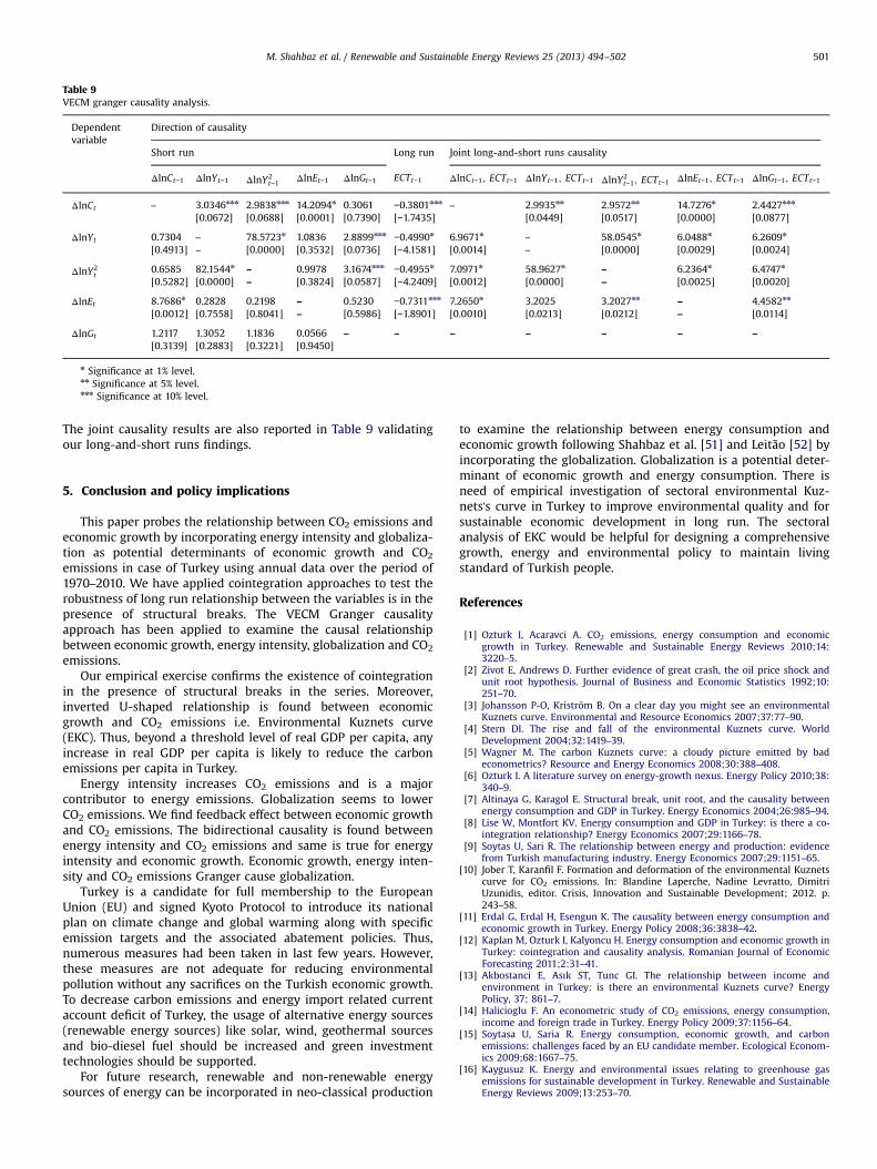
The presence of cointegration among the variables implies thatcausality relation must exist at least from one side. The directionalrelationship between energy intensity, economic growth, globali-zation and CO2 emissions will provide help in articulating com-prehensive policy to sustain economic growth by controllingenvironment from degradation and utilizing energy efficienttechnologies imported from advanced countries. We appliedGranger causality test within the VECM framework to detect thecausality between the variables. Table 9 reports the results of theVECM Granger causality analysis. The long run causality is cap-tured by a significant t-test on a negative coefficient of the lagged

error-correction term ECMt−1. The jointly significant LR test on thelagged explanatory variables shows short-run causality.

Table 9 reveals that the estimates of ECMt−1 are having negativesigns and statistically significant in all the VECMs. The significanceof lagged error term shows speed of adjustment from short runtoward long run equilibrium path in the equation of energyconsumption (−0.7311), economic growth (−0.4990, −0.4955) aswell as CO2 emissions (−0.3801). This implies that the VECMequation of energy intensity has high speed of adjustment(−0.7311) as compared to economic growth (−0.4990, −0.4955)and CO2 emissions (−0.3801) the VECMs.

The long run causality result reported that the feedback effectis found between economic growth and CO2 emissions. Thisimplies that Turkey is achieving economic growth at the cost ofenvironment. The bidirectional causality is found between energyintensity and CO2 emissions. This suggests adopting energy-efficient technology to enhance production which emits less CO2

emissions. The feedback effect also exists between economicgrowth and energy intensity.

This reveals that energy is an important stimulant like otherfactor of production and reduction in energy consumption wouldretard economic growth. This finding supports for energy explora-tion policies to sustain economic growth for long run. Globaliza-tion Granger causes economic growth, energy intensity and CO2

emissions validating the globalization-led growth, globalization-led energy and globalization-led CO2 emissions hypotheses.

The results of short run causality are very interesting. Theneutral effect is found between CO2 emissions and globalizationand, the same is true for energy intensity and globalization.Economic growth Granger causes CO2 emissions. The feedbackeffect exists between energy intensity and CO2 emissions. Thereis no causality between energy intensity and economic growth.

Table 9VECM granger causality analysis.

Dependentvariable

Direction of causality

Short run Long run Joint long-and-short runs causality

ΔlnCt−1 ΔlnYt−1 ΔlnY2t−1

ΔlnEt−1 ΔlnGt−1 ECTt−1 ΔlnCt−1 ; ECTt−1 ΔlnYt−1 ; ECTt−1 ΔlnY2t−1; ECTt−1 ΔlnEt−1 ; ECTt−1 ΔlnGt−1 ; ECTt−1

ΔlnCt – 3.0346nnn 2.9838nnn 14.2094n 0.3061 −0.3801nnn – 2.9935nn 2.9572nn 14.7276n 2.4427nnn

[0.0672] [0.0688] [0.0001] [0.7390] [−1.7435] [0.0449] [0.0517] [0.0000] [0.0877]

ΔlnYt 0.7304 – 78.5723n 1.0836 2.8899nnn −0.4990n 6.9671n – 58.0545n 6.0488n 6.2609n

[0.4913] – [0.0000] [0.3532] [0.0736] [−4.1581] [0.0014] – [0.0000] [0.0029] [0.0024]

ΔlnY2t

0.6585 82.1544n – 0.9978 3.1674nnn −0.4955n 7.0971n 58.9627n – 6.2364n 6.4747n

[0.5282] [0.0000] – [0.3824] [0.0587] [−4.2409] [0.0012] [0.0000] – [0.0025] [0.0020]

ΔlnEt 8.7686n 0.2828 0.2198 – 0.5230 −0.7311nnn 7.2650n 3.2025 3.2027nn – 4.4582nn

[0.0012] [0.7558] [0.8041] – [0.5986] [−1.8901] [0.0010] [0.0213] [0.0212] – [0.0114]

ΔlnGt 1.2117 1.3052 1.1836 0.0566 – – – – – – –

[0.3139] [0.2883] [0.3221] [0.9450]

n Significance at 1% level.nn Significance at 5% level.nnn Significance at 10% level.

M. Shahbaz et al. / Renewable and Sustainable Energy Reviews 25 (2013) 494–502 501

The joint causality results are also reported in Table 9 validatingour long-and-short runs findings.

5. Conclusion and policy implications

This paper probes the relationship between CO2 emissions andeconomic growth by incorporating energy intensity and globaliza-tion as potential determinants of economic growth and CO2

emissions in case of Turkey using annual data over the period of1970–2010. We have applied cointegration approaches to test therobustness of long run relationship between the variables is in thepresence of structural breaks. The VECM Granger causalityapproach has been applied to examine the causal relationshipbetween economic growth, energy intensity, globalization and CO2

emissions.Our empirical exercise confirms the existence of cointegration

in the presence of structural breaks in the series. Moreover,inverted U-shaped relationship is found between economicgrowth and CO2 emissions i.e. Environmental Kuznets curve(EKC). Thus, beyond a threshold level of real GDP per capita, anyincrease in real GDP per capita is likely to reduce the carbonemissions per capita in Turkey.

Energy intensity increases CO2 emissions and is a majorcontributor to energy emissions. Globalization seems to lowerCO2 emissions. We find feedback effect between economic growthand CO2 emissions. The bidirectional causality is found betweenenergy intensity and CO2 emissions and same is true for energyintensity and economic growth. Economic growth, energy inten-sity and CO2 emissions Granger cause globalization.

Turkey is a candidate for full membership to the EuropeanUnion (EU) and signed Kyoto Protocol to introduce its nationalplan on climate change and global warming along with specificemission targets and the associated abatement policies. Thus,numerous measures had been taken in last few years. However,these measures are not adequate for reducing environmentalpollution without any sacrifices on the Turkish economic growth.To decrease carbon emissions and energy import related currentaccount deficit of Turkey, the usage of alternative energy sources(renewable energy sources) like solar, wind, geothermal sourcesand bio-diesel fuel should be increased and green investmenttechnologies should be supported.

For future research, renewable and non-renewable energysources of energy can be incorporated in neo-classical production

to examine the relationship between energy consumption andeconomic growth following Shahbaz et al. [51] and Leitão [52] byincorporating the globalization. Globalization is a potential deter-minant of economic growth and energy consumption. There isneed of empirical investigation of sectoral environmental Kuz-nets's curve in Turkey to improve environmental quality and forsustainable economic development in long run. The sectoralanalysis of EKC would be helpful for designing a comprehensivegrowth, energy and environmental policy to maintain livingstandard of Turkish people.

References

[1] Ozturk I, Acaravci A. CO2 emissions, energy consumption and economicgrowth in Turkey. Renewable and Sustainable Energy Reviews 2010;14:3220–5.

[2] Zivot E, Andrews D. Further evidence of great crash, the oil price shock andunit root hypothesis. Journal of Business and Economic Statistics 1992;10:251–70.

[3] Johansson P-O, Kriström B. On a clear day you might see an environmentalKuznets curve. Environmental and Resource Economics 2007;37:77–90.

[4] Stern DI. The rise and fall of the environmental Kuznets curve. WorldDevelopment 2004;32:1419–39.

[5] Wagner M. The carbon Kuznets curve: a cloudy picture emitted by badeconometrics? Resource and Energy Economics 2008;30:388–408.

[6] Ozturk I. A literature survey on energy-growth nexus. Energy Policy 2010;38:340–9.

[7] Altinaya G, Karagol E. Structural break, unit root, and the causality betweenenergy consumption and GDP in Turkey. Energy Economics 2004;26:985–94.

[8] Lise W, Montfort KV. Energy consumption and GDP in Turkey: is there a co‐integration relationship? Energy Economics 2007;29:1166–78.

[9] Soytas U, Sari R. The relationship between energy and production: evidencefrom Turkish manufacturing industry. Energy Economics 2007;29:1151–65.

[10] Jober T, Karanfil F. Formation and deformation of the environmental Kuznetscurve for CO2 emissions. In: Blandine Laperche, Nadine Levratto, DimitriUzunidis, editor. Crisis, Innovation and Sustainable Development; 2012. p.243–58.

[11] Erdal G, Erdal H, Esengun K. The causality between energy consumption andeconomic growth in Turkey. Energy Policy 2008;36:3838–42.

[12] Kaplan M, Ozturk I, Kalyoncu H. Energy consumption and economic growth inTurkey: cointegration and causality analysis. Romanian Journal of EconomicForecasting 2011;2:31–41.

[13] Akbostanci E, Asık ST, Tunc GI. The relationship between income andenvironment in Turkey: is there an environmental Kuznets curve? EnergyPolicy, 37; 861–7.

[14] Halicioglu F. An econometric study of CO2 emissions, energy consumption,income and foreign trade in Turkey. Energy Policy 2009;37:1156–64.

[15] Soytasa U, Saria R. Energy consumption, economic growth, and carbonemissions: challenges faced by an EU candidate member. Ecological Econom-ics 2009;68:1667–75.

[16] Kaygusuz K. Energy and environmental issues relating to greenhouse gasemissions for sustainable development in Turkey. Renewable and SustainableEnergy Reviews 2009;13:253–70.

M. Shahbaz et al. / Renewable and Sustainable Energy Reviews 25 (2013) 494–502502

[17] Jobert T, Karanfil F, Tykhonenko A. Environmental Kuznets curve for carbondioxide emissions: lack of robustness to heterogeneity? Working paper.Université Nice Sophia Antipolis.

[18] Joberta T, Karanfil K. Sectoral energy consumption by source and economicgrowth in Turkey. Energy Policy 2007;35:5447–56.

[19] Lisea W. Decomposition of CO2 emissions over 1980–2003 in Turkey. EnergyPolicy 2006;34:1841–52.

[20] Ozturk I, Kaplan M, Kalyoncu H. The causal relationship between energyconsumption and GDP in Turkey. Energy & Environment 2013 [forthcoming].

[21] Grossman GM, Krueger AB. Environmental impacts of a North American freetrade agreement. NBER working paper 3914; November 1991.

[22] Dinda S. Impact of globalization on environment: how do we measure andanalyze it? In: Proceedings of ISEE 2006; 2008

[23] Shahbaz M, Lean HH, Shabbir MS. Environmental Kuznets curve hypothesis inPakistan: cointegration and Granger causality. Renewable and SustainableEnergy Reviews 2012;16:2947–53.

[24] Wheeler D. Racing to the bottom? Foreign investment and air quality indeveloping countries. World Bank working paper; 2000.

[25] Copeland BR, Taylor MS. Trade and environment: a partial synthesis. AmericanJournal of Agricultural Economics 1995;77:765–71.

[26] Copeland BR, Taylor MS. Trade growth and the environment. Journal ofEconomic Literature 2004;42:7–71.

[27] Birdsall N, Wheeler D. Trade Policy and Industrial Pollution in Latin America:Where Are the Pollution Havens? The Journal of Environment Development1993;2(1):137–49.

[28] Lee H, Roland-Holst D. The environment and welfare implications of trade andtax policy. Journal of Development Economics 1997;52:65–82.

[29] Jones LE, Rodolfo EM. A positive model of growth and pollution controls. NBERworking paper 5205; 1995.

[30] Antweiler W, Copeland BR, Taylor MS. Is free trade good for the environment?American Economic Review 2001;91:877–908.

[31] Liddle B. Free trade and the environment-development system. EcologicalEconomics 2001;39:21–36.

[32] Dean JM. Testing the impact of trade liberalization on the environment:theory and evidence. Canadian Journal of Economics 2002;35:819–42.

[33] Magani S. Trade liberalization and the environment: carbon dioxide for 1960–1999. Economics Bulletin 2004;17:1–5.

[34] McAusland C. Trade, politics, and the environment: tailpipe vs. smokestack.Journal of Environmental Economics and Management 2008;55:52–71.

[35] Frankel JA. Environmental effects of international trade. 2009 Expert reportno. 31 to Sweden's Globalisation Council.

[36] Dreher A. Does globalization affect growth? Evidence from a new index ofglobalization Applied Economics 2006;38:1091–110.

[37] Shahbaz M, Mutascu M, Azim P. Environmental Kuznets curve in Romania andthe role of energy consumption. Renewable and Sustainable Energy Reviews2013;18:165–73.

[38] Dickey DA, Fuller WA. Distribution of the estimators for autoregressive timeseries with a unit root. Journal of American Statistical Association 1979;74:427–31.

[39] Phillips PCB, Perron P. Testing for a unit root in time series regression.Biometrika 1988;75:335–46.

[40] Kwiatkowski D, Phillips P, Schmidt P, Shin Y. Testing the null hypothesis ofstationary against the alternative of a unit root: how sure are we thateconomic time series have a unit root? Journal of Econometrics 1992;54:159–78.

[41] Elliot G, Rothenberg TJ, Stock JH. Efficient tests for an autoregressive unit root.Econometrica 1996;64:813–36.

[42] Ng S, Perron P. Lag length selection and the construction of unit root test withgood size and power. Econometrica 2001;69:1519–54.

[43] Sen A. On unit root tests when the alternative is a trend break stationaryprocess. Journal of Business and Economic Statistics 2003;21:174–84.

[44] Pesaran MH, Shin Y, Smith R. Bounds testing approaches to the analysis oflevel relationships. Journal of Applied Econometrics 2001;16:289–326.

[45] Lütkepohl H. Structural vector autoregressive analysis for cointegrated vari-ables. AStA Advances in Statistical Analysis 2006;90:75–88.

[46] Johansen S, Juselies K. Maximum likelihood estimation and inferences oncointegration. Oxford Bulletin of Economics and Statistics 1990;52:169–210.

[47] Narayan PK. The savings and investment nexus for China: evidence fromcointegration tests. Applied Economics 2005;37:1979–90.

[48] Gregory AW, Hansen BE. Residual-based tests for cointegration in models withregime shifts. Journal of Econometrics 1996;70:99–126.

[49] Shahbaz M. Does trade openness affect long run growth? Cointegration,causality and forecast error variance decomposition tests for Pakistan Eco-nomic Modelling 2012;29:2325–39.

[50] Leow YGA. Reexamination of the exports in Malaysia's economic growth: afterAsian financial crisis, 1970–2000. International Journal of ManagementSciences 2004;11:79–204.

[51] Shahbaz M, Zeshan M, Afza T. Is energy consumption effective to spureconomic growth in Pakistan? New evidence from bounds test to levelrelationships and Granger causality tests Economic Modelling 2012;29:2310–9.

[52] Leitão NC. The environmental Kuznets curve and globalization: the empiricalevidence for Portugal, Spain, Greece and Ireland. Energy Economics Letters2013;1:15–23.