www.cbo.gov/publication/57089 Working Paper Series Congressional Budget Office Washington, D.C. Revisiting the Extent to Which Payroll Taxes Are Passed Through to Employees Dorian Carloni Congressional Budget Office [email protected]Working Paper 2021-06 June 2021 To enhance the transparency of the work of the Congressional Budget Office and to encourage external review of that work, CBO’s working paper series includes papers that provide technical descriptions of official CBO analyses as well as papers that represent independent research by CBO analysts. Papers in this series are available at http://go.usa.gov/xUzd7. I thank Andreas Lichter of the Heinrich Heine University Düsseldorf, Andreas Peichl of the University of Munich, and Sebastian Siegloch of the University of Mannheim for generously providing data on estimates of own-wage labor demand elasticities for the United States. I am grateful to Jaeger Nelson and Kerk Phillips for their invaluable assistance with CBO’s overlapping generations model and to Wendy Edelberg (formerly of CBO), Jeffrey Kling, John McClelland, James Pearce, and Joseph Rosenberg for helpful comments and suggestions. I also thank Paul Kindsgrab of the University of Michigan, Greg Leiserson of the Washington Center for Equitable Growth, Barra Roantree of the Economic and Social Research Institute, David Splinter of the Joint Committee on Taxation, and Alan Viard of the American Enterprise Institute. Although those experts provided considerable assistance, they are not responsible for the contents of this paper. Rebecca Lanning was the editor.
Payroll taxes are the second largest source of federal tax revenues in the United States after
individual income taxes. Federal payroll taxes, which are collected to finance Social Security,
Medicare, and unemployment insurance, raised $1.2 trillion in 2019, or 5.8 percent of gross
domestic product (GDP) and 35.9 percent of total tax revenues (CBO 2020a). Because payroll taxes
are such a large source of tax revenues, estimates of the extent to which those taxes do or do not get
shifted to employees have important implications for evaluating the effects of such taxes on
employment, the distribution of income, and economic growth. For example, if employers shifted
most of the burden of a higher payroll tax to their employees through lower after-tax wages,
reductions in labor demand would probably be limited. A large pass-through of the tax to wages
rather than to other forms of income also affects estimates of how after-tax income is distributed
among households because wages are distributed differently than those other forms of income. In
addition, to the extent that business profits and investment are causally linked, a large pass-through
of the tax to employees that has small effects on employers and profits implies that a payroll tax
change would have less effect on economic growth.
Traditionally, economists project that payroll taxes are fully borne by employees through lower
wages, at least in the long run. But empirical research on the relationship between payroll tax
changes and employees’ compensation in the United States is limited, is focused on changes in state
unemployment benefits or employer-provided health insurance and is probably not generalizable to
changes in U.S. federal payroll taxes. By contrast, the empirical literature on payroll tax incidence
in other countries is more developed and often shows less than full pass-through of payroll tax
changes to employees, but that evidence is not directly applicable to the United States because of
differences in those countries’ institutional settings.
In this paper, I combine theory and existing empirical evidence to revisit the extent to which payroll
taxes are passed through to employees and to contribute to the discussion on the incidence of U.S.
federal payroll tax changes. Like the rest of the theoretical literature on the topic, this paper
considers the burden of payroll taxes in isolation, therefore ignoring the effect of payroll tax
changes on future Social Security benefits. My estimates, which rely on stylized models and vary
among those models, are useful for highlighting important determinants of payroll tax incidence but
do not account for the details of a specific payroll tax proposal. I complement those model-based
estimates with a discussion of the empirical literature on payroll tax incidence. That literature is
useful both to highlight the methods used when estimating payroll tax incidence empirically and to
illustrate additional factors that can affect the incidence of a specific payroll tax proposal on
employees. For example, that literature shows that both the statutory incidence and the direction of
payroll tax changes can affect the share of the burden on employees.
First, I develop a partial equilibrium model and rely on short-run labor elasticities to estimate the
short-run incidence of payroll tax changes on employees. That model is an extension of the model
2
used for evaluating the incidence of changes in proportional ad valorem taxes and can also be used
for determining the effects on households’ well-being (that is, the welfare effects) of changes in
other nonlinear taxes in perfectly competitive markets. I rely on that model, a sample of publicly
available tax returns, and estimates of short-run labor supply and demand elasticities to estimate the
incidence of changes in Federal Insurance Contributions Act (FICA) taxes and exclusions from the
payroll tax base. That approach finds that the portion of the tax burden from payroll taxes that falls
on labor varies significantly among different hypothetical policy changes. Specifically, I estimate
that 58 percent of the additional tax burden created by an increase in the hospital insurance (HI) tax
rate would be on employees. The predicted additional tax burden on employees for tax changes that
apply only to a fraction of taxable earnings would vary: I estimate that 23 percent of the tax burden
from an increase in the additional Medicare surtax rate and 62 percent of the tax burden from an
increase in the Old-Age, Survivors, and Disability Insurance (OASDI) rate would be shifted to
employees in the short run. By contrast, increases in payroll tax liability resulting from changes in
taxable earnings thresholds or in the share of total compensation that is taxable would be associated
with more than full pass-through of the tax to employees. Unlike increases in tax rates, such
changes are associated with increased labor supply, which further reduces wages, therefore
increasing the tax burden on employees.
Second, I discuss the long-run effects of payroll tax changes on employees using a general
equilibrium model: the Congressional Budget Office’s overlapping generations (OLG) model. In
that model, I estimate the incidence of payroll tax changes on employees from changes in
employees’ after-tax wages and the marginal product of capital. In that model, hypothetical payroll
tax increases would reduce employees’ after-tax wages, but the long-run incidence of those tax
increases on employees would depend on how the revenues are used and the overall
macroeconomic effects. For example, employees would bear less than the full burden of an increase
in the HI tax rate if the revenues raised were used to reduce government debt. In that case,
additional payroll taxes would reduce households’ disposable income, which would reduce private
savings, but the stock of productive capital would increase because more private wealth would be
invested in productive capital rather than in government debt. That would reduce the marginal
product of capital. By contrast, employees would bear more than the full burden of an increase in
the HI tax rate if the revenues raised were used to increase noninvestment government spending.
The stock of productive capital would decrease in that case, increasing the marginal return on
capital. To illustrate the differential effects of payroll tax changes, I then estimate the incidence of
various hypothetical payroll tax changes when the revenues raised are used to increase
noninvestment government spending. Under such a revenue recycling policy, employees would bear
more than the full burden of the payroll tax changes considered.
I relate those model-based estimates to the empirical literature on payroll tax incidence, which helps
illustrate additional determinants of payroll tax incidence. That literature, which is largely focused
on the short-run incidence of changes in payroll tax rates in other countries, finds that the statutory
incidence of a payroll tax change can matter and that rigidities in the labor market can contribute to
3
asymmetric burdens of payroll tax changes on employees. In addition, those studies find that the
perceived future benefits associated with payroll tax increases, the way the tax is designed and
remitted, the degree of firms’ market power, the state of the economy, and a country’s social norms
are all important contributors to the incidence of payroll taxes. The insights from that literature are a
useful complement to the model-based estimates of the paper when evaluating the incidence of
specific payroll tax proposals.
Estimating Payroll Tax Incidence After a Tax Change
The existing empirical evidence on payroll tax incidence is unlikely to apply to changes in U.S.
federal payroll taxes. That is because it relates to changes in employer-provided benefits (which are
often described as “benefit taxes”) or changes in state-level payroll taxes in the United States or
because it focuses on other countries, where the institutional setting is generally different.1 Despite
those differences, the existing literature offers useful guidance for understanding how to estimate
payroll tax incidence, and it is a useful starting point to help frame the rest of the analysis presented
in this paper.
That literature emphasizes that changes in employees’ after-tax wages, the main outcome
considered when estimating the incidence of payroll tax changes on employees, can result directly
from changes in payroll taxes but also from changes in hours worked, intensity of work, shifting
between forms or the timing of compensation, and evasion responses. Some of those adjustment
margins are challenging to measure but also important for a broad measure of incidence. In
addition, the literature discusses how to separate the effects of payroll tax changes on wages from
changes in employment that result from behavioral responses. Separating those effects requires
somewhat restrictive assumptions when information on hours worked is unavailable, such as with
tax data, but is necessary for determining the incidence of payroll tax changes on employees.
Finally, the literature emphasizes the challenges of measuring long-run incidence and, therefore,
generally focuses on the short-run incidence of payroll tax changes.2
Computing the Overall Incidence on Employees
Computing the overall incidence of a tax change on employees is challenging because some
margins of adjustments in employees’ wages are difficult to measure. For example, margins of
adjustments such as changes in employees’ intensity of work or changes in the timing and forms of
compensation (some of which are untaxed) affect employees’ wages but are generally not
1 For evidence that employer-sponsored insurance benefits result in lower wages, see Gruber (1994), Baicker and
Chandra (2006), and Kolstad and Kowalski (2016). For evidence on the incidence of State Unemployment Tax Act
taxes, see Anderson and Meyer (1997) and Anderson and Meyer (2000).
2 In this paper, compensation is used to denote all employee compensation, whereas earnings and taxable
compensation are used to denote taxable compensation. Similarly, hourly compensation includes all forms of
compensation on an hourly basis, whereas hourly earnings and gross hourly wages indicate hourly taxable
compensation. Net hourly wages is used to define hourly earnings net of the taxes paid.
4
considered in empirical estimates. Therefore, to the extent that changes in the intensity of work per
hour produce changes in wages, ignoring changes along that margin could bias existing incidence
estimates. A shift in the form of compensation from taxable to nontaxable (or vice versa) or in the
timing of compensation can also affect wages.3 For example, employers could adjust to a payroll tax
change by paying more of their employees’ compensation in untaxed fringe benefits or by shifting
the payment of that compensation from one year to another. Because those margins of adjustment
are challenging to measure, the empirical literature has largely focused on changes in employees’
hourly taxable earnings and on how to separate that effect (that is, the incidence of the tax) from the
additional effects of changes in hours worked on taxable compensation.
Separating the Incidence of a Tax Change From Changes in Hours Worked
When the incidence of a tax change on hourly earnings is different from the statutory incidence of
the tax, it is empirically challenging to separate that effect of the tax on hourly earnings from the
effect of changes in hours worked on employees’ earnings.4 When information on hours worked is
unavailable, separating the two effects is possible only with estimates of the magnitude of the pass-
through to employees’ hourly earnings or the size of behavioral responses. When information on
hours worked is available, a significantly less structural approach is necessary. In that case, only
assumptions about responses other than changes in hours worked are necessary to separate the
direct effect of the tax change from the additional effects of behavioral responses on employees’
earnings.
No Information Available on Hours Worked. In this case, estimates of the incidence of the tax
change on hourly earnings or the size of behavioral responses are necessary to separate those two
effects. The empirical literature generally projects that the incidence of payroll tax changes is fully
reflected in employees’ hourly earnings, so that observed changes in taxable earnings can be
interpreted as resulting from labor supply substitution and income effects. The incidence of the
payroll tax change on hourly earnings is therefore a parameter in the model’s structure that is
projected on the basis of information from other sources rather estimated directly. Alternatively,
information from other sources could be used to estimate the effects of changes in hours worked
and to estimate the resulting incidence of the tax change from changes in employees’ earnings.
Information Available on Hours Worked. The incidence of the tax change and the magnitude of
changes in hours worked can be estimated simultaneously in this case, because changes in taxable
earnings can be decomposed into changes in hours worked and changes in hourly earnings. Changes
in hours worked reflect behavioral responses from the employee, the employer, or both and take
into account both substitution and income effects. In that case, changes in hourly earnings are an
3 For additional discussion on this point, see Auten et al. (2016).
4 For a discussion of the challenges of separating behavioral changes to labor supply from incidence in the context of
payroll tax changes, see Adam et al. (2019). Incidence in the context of individual income taxes is discussed in Saez
et al. (2012b).
5
accurate measure of the incidence of the tax unless those changes are driven by changes in
employees’ effort per hour worked or there are adjustments to employees’ compensation other than
changes in their taxable earnings. If adjustments along those other dimensions occur, the change in
hourly earnings offers an incomplete measure of the overall incidence of the tax change on
employees.
Distinguishing Between Short-Run and Long-Run Incidence
Because of data constraints, most existing empirical studies on payroll tax incidence focus on short-
run incidence and generally consider changes in hourly wages in the first five years after a tax
change. Long-run incidence, which can be estimated with theoretical models, is less often discussed
but can be different.5 For example, employers might more easily adjust their demand for labor and
their employees’ hours worked in the long run than in the short run. Employers might also be
unable to change their employees’ hourly wages and their inputs of production in the short run.6
Employees’ preferences for the type of compensation received might also differ in the short run and
the long run. For example, employees can respond to an announced tax change by asking for
additional compensation to be paid in years before the introduction of the tax change. That response
would probably disappear in the long run if the tax change was permanent. Finally, other short-term
frictions in the labor market can explain differences in estimated substitution elasticities between
studies and create a wedge between short-run and long-run incidence.7 Those frictions can, for
example, relate to adjustment costs and wage misperceptions.
Using Partial Equilibrium Models to Quantify the Welfare Effects of
Payroll Tax Changes
Because of the limited empirical evidence on the incidence of payroll tax changes in the United
States, the welfare effects of changes in federal payroll taxes are also challenging to estimate.
Economic models can be used to quantify those effects.8 Partial equilibrium models of tax incidence
can be used to quantify the welfare effects of tax changes when considering the effects of the tax
change in the market where the tax is introduced. General equilibrium models also consider the
effects of the tax change in other markets and, although they involve a more complex modeling
structure and have limitations, are useful for evaluating the long-run incidence of tax changes.
In partial equilibrium models the burden of the tax is split between the demand and supply sides of
the market, and that split depends on the relative magnitude of the supply and demand elasticities.
5 See Saez et al. (2012a) for a discussion of long-term incidence.
6 See Hamermesh (1993) for a discussion of labor demand elasticities.
7 For a detailed discussion of the importance of labor market frictions on labor supply elasticities, see Chetty (2012).
8 For example, general equilibrium models are often used to discuss the incidence of corporate income tax changes
on labor and capital. For a recent review of that literature, see Gravelle (2010).
6
For example, the extent to which the burden of a payroll tax change falls on employees is
determined by focusing on the effects of the tax in the labor market and depends on how employees
adjust their labor supply in response to that change, as well as how their employers adjust their
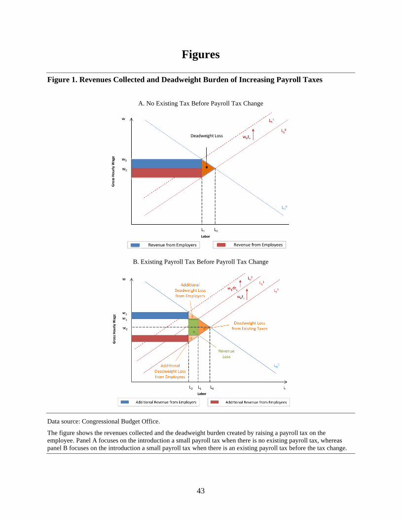
demand for labor.9 When there is no existing tax, the tax revenues raised equal the tax collected on
each employee times the labor employed, as shown in panel A of Figure 1. Because distortions of
behavior and the resulting deadweight burden of the tax are small in such cases, the burden of the
additional tax revenues collected on employees and employers can be approximated by the first-
order welfare effects of the tax on each side of the market.10 The tax revenues collected fall partly
on employees’ wages and partly on employers’ profits. Instead, when a tax is already in place
before a tax change, the marginal deadweight burden of a tax increase can potentially be large
because the revenue loss from labor that is no longer taxed is larger, as shown in panel B of
Figure 1. If that reduction in the existing tax revenues is not associated with a corresponding
decrease in government spending, which is typically assumed when distributing a tax change in
isolation, the same framework can be used to assess the incidence of a tax change when a tax is
already in place.
Partial equilibrium models focus on one market at a time and therefore ignore adjustments in other
markets. A partial equilibrium model of tax incidence focusing on the labor market ignores
adjustments in other input markets and in final goods markets, all of which can influence the share
of the tax burden on employees. For example, employers could increase consumer prices because of
the tax, which could change the relative price of consumption for employees, employers, and other
consumers, as well as the overall incidence of the tax. That would occur if prices increased for some
commodities but not others and if different groups had different consumption bundles. If so, some
burden of the tax would be shifted from the groups facing a smaller increase in the price of their
consumption bundles to the groups facing a larger price increase in their consumption bundles. If
every consumer was characterized by the same consumption bundle or if the percentage increase in
consumer prices was the same for all commodities, then higher prices would not contribute to
reallocating the tax burden from some groups to other groups.11
9 That general principle holds for both per-unit taxes and ad valorem taxes such as payroll taxes and for both
perfectly competitive labor markets and markets with imperfect competition. For a review of the theoretical
literature on tax incidence, see Fullerton and Metcalf (2002). For a discussion of incidence in markets with imperfect
competition, see Weyl and Fabinger (2013). For a discussion of incidence theory applied to distributional analysis,
see Leiserson (2020).
10 The deadweight burden of a tax, defined as the welfare loss (measured in dollars) created by a tax over and above
the tax revenues generated by the tax, is small in this case because changes in quantities are small. For a discussion
of the efficiency costs of taxation, see Auerbach and Hines (2002).
11 Differences in the pass-through of payroll tax changes to consumer prices in commodity markets are challenging
to quantify. Differences in consumption bundles among consumers are also difficult to measure empirically, largely
because it would be challenging to separate employees, employers, and other consumers.
7
Partial equilibrium models of incidence, like general equilibrium models, also ignore the effects of
behavioral responses along a set of dimensions, some of which can affect revenues. For example,
the following margins of adjustment are ignored when focusing on the labor market. First, those
models do not account for shifting between taxable and nontaxable forms of compensation, which
would affect the total revenues raised by the tax but also the distribution of the tax burden. For
example, if employers decreased both taxable and nontaxable compensation as payroll taxes were
increased, the share of the burden on employees would be larger than estimated in this paper.
Second, partial equilibrium models ignore intertemporal shifting of taxable compensation and other
forms of avoidance or evasion responses, which would also affect tax revenues collected and the
distribution of the burden. For example, focusing on employees’ higher current compensation but
ignoring their lower future compensation would lead to overstating the benefit they receive from a
payroll tax cut. Finally, those models ignore changes in employees’ effort per hour worked, which
can also be adjusted in response to a tax change and can affect the gross hourly wage, therefore
changing the distribution of the burden. Although that greater effort imposes a nonmonetary burden
on employees, ignoring increases in wages from greater effort would lead to understating the burden
on employees as payroll taxes are increased.
A Stylized Partial Equilibrium Model of Tax Incidence for a
Proportional Payroll Tax
The simplest incidence model for payroll taxes incorporates the assumptions of perfectly
competitive labor markets, no labor market frictions, and proportional payroll tax rates on all forms
of compensation. In that market, employers’ demand for labor equals employees’ supply of labor,
and the gross hourly wage is set for that condition to be satisfied.12 Both employers and employees
take gross hourly wages as given and choose how much labor to employ or supply. Employers base
their employment decisions on their average labor cost, 𝑤𝑑 = 𝑤(1 + 𝑡𝑑), which depends on the
gross hourly wage w paid to their employees and on the payroll tax td levied on employers.
Employees decide how much labor to supply on the basis of their net hourly wage, 𝑤𝑠 = 𝑤(1 − 𝑡𝑠),
which depends on their gross hourly wage and the payroll tax ts levied on employees.
Increase in Payroll Taxes Levied on Employers
When the payroll tax levied on employers is increased, they can shift some of the additional tax
burden to employees by reducing gross hourly wages. That reduction in gross hourly wages is larger
when an employer’s labor demand elasticity (which is negative: 𝜀𝐷 ≤ 0) is higher in absolute
value—that is, when the employer reduces demand for labor more dramatically as labor costs
increase. That reduction in gross hourly wages is also larger when employees’ labor supply
elasticity (which is positive: 𝜀𝑆 ≥ 0) is lower—that is, when employees are less willing to reduce
12 Throughout the analysis, employers denote a broad category that includes factors of production other than labor,
which are capital, land, and nonland pure rents.
8
employment as their net earnings are cut. The increase in employers’ labor costs is a function of the
statutory burden of the tax, which is on employers, and the relative slope of the labor demand and
labor supply elasticities, which determines how much of that statutory burden gets shifted to
employees through reductions in gross hourly wages:
𝑑𝑤𝑑𝑑𝑡𝑑
=𝑑𝑤
𝑑𝑡𝑑(1 + 𝑡𝑑) + 𝑤 = 𝑤
𝜀𝑆(𝜀𝑆 − 𝜀𝐷)
≥ 0
The payroll tax raises additional tax revenues, which include the additional revenues collected on
existing wages and the revenue loss from lower gross wages. The share of the tax burden on
employers is equal to the ratio between the change in employers’ hourly labor costs and the
additional tax revenues raised. The share of the burden on employees is equal to 1, minus the share
of that burden: 13
𝑆𝐻𝐵𝑠 = −𝜀𝐷
𝜀𝑆 (1+𝑡𝑑1 − 𝑡𝑠
) − 𝜀𝐷
Therefore, the model predicts that employers’ ability to shift part of the statutory burden of the tax
to employees through lower gross hourly wages, which determines the welfare effects and the
incidence of the tax change, depends on labor demand and labor supply elasticities, as well as the
existing payroll tax rates on employers and employees.
Increase in Payroll Taxes Levied on Employees
Instead, when the payroll tax levied on employees is increased, they can shift some of that
additional statutory burden to their employers by negotiating higher gross hourly wages. That
increase in gross wages is higher when the employers’ labor demand elasticity (which is negative:
𝜀𝐷 ≤ 0) is lower in absolute value or when the employees’ labor supply elasticity (which is
positive: 𝜀𝑆 ≥ 0) is higher. The overall reduction in employees’ net hourly wages depends on that
additional statutory burden, which reduces their net hourly wages, and the relative slope of the labor
demand and labor supply elasticities, which determines how much of that statutory burden gets
shifted to employers through higher gross hourly wages:
𝑑𝑤𝑠𝑑𝑡𝑠
=𝑑𝑤
𝑑𝑡𝑠(1 − 𝑡𝑠) − 𝑤 = 𝑤
𝜀𝐷(𝜀𝑆 − 𝜀𝐷)
≤ 0
13 See the appendix for a derivation of this formula. If there are no initial payroll taxes, the formula simplifies to
𝑆𝐻𝐵𝑠 = −𝜀𝐷
(𝜀𝑆−𝜀𝐷). Whether or not there is an existing tax in place, the incidence of the tax change depends on the
ratio of the slopes of the demand and supply curves. With an existing tax in place, that is the ratio between
𝜀𝑆/[𝑤(1 − 𝑡𝑠] and 𝜀𝐷/[𝑤
1+𝑡𝑑].
9
The payroll tax raises additional revenues, which include the additional revenues collected on
existing gross wages and the revenues collected from higher gross wages. The share of the
additional tax burden on employees is equal to the ratio between the change in employees’ net
hourly wage and the change in payroll tax revenues. As for changes in payroll taxes levied on
employers, the share of the tax burden on employees depends on labor demand and labor supply
elasticities, as well as the existing payroll tax rates on employers and employees:
𝑆𝐻𝐵𝑠 = −𝜀𝐷
𝜀𝑆 (1+𝑡𝑑1 − 𝑡𝑠
) − 𝜀𝐷
Conditions Under Which Employees Bear the Full Burden of the Tax Change
In this simplified model, unlike models in which employers earn limited or no profits, employers
generally bear some of the additional tax burden created by the tax change through lower profits.
Employees bear the full burden of the additional tax only under very specific conditions. They bear
the full burden if they do not adjust their labor supply in response to changes in their net wages—
that is, if the labor supply is fully inelastic (𝜀𝑆 = 0). Employees also bear the full burden of the tax
if employers make large adjustments to their labor demand in response to changes in their labor
costs—that is, if their labor demand is fully elastic (𝜀𝐷 = −∞). In such cases, changes in payroll
taxes levied on employers are shifted entirely to employees through lower gross hourly wages, and
changes in payroll taxes levied on employees are not offset by changes in gross hourly wages. In
either case, an increase of 1 percentage point in the payroll tax rate is associated with a 1 percent
decrease in employees’ net hourly wages and no change in employers’ labor costs.
A Framework for Estimating Payroll Tax Incidence in the
United States
The framework derived above helps lay out the main determinants of payroll tax incidence but
relies on a simplified tax schedule, in which payroll taxes are imposed proportionally on employees’
compensation, and all compensation is taxed. By contrast, U.S. federal payroll taxes are generally
not imposed proportionally on employees’ earnings and exclude some components of
compensation.14 Specifically, payroll taxes on employed workers (FICA taxes) have two main
components: the OASDI tax and the HI tax. The OASDI tax is 12.4 percent (split equally between
the employee and employer) and applies to taxable compensation up to a maximum base ($128,400
in 2018) that is indexed to the growth in average wages. The HI tax is 2.9 percent (also split equally
between the employee and employer) and is imposed on all earnings. An additional Medicare tax of
0.9 percent is imposed on the employee for taxable compensation above a threshold that varies by
14 FICA taxes are levied on salaries, fees, bonuses, and commissions but also on other forms of compensation, such
as tips and gratuities, employee expenses paid through a nonaccountable plan or in excess of per diem rates, and
severance and strike benefits. They also apply to taxable fringe benefits, such as cars and other goods and low-
interest loans provided to employees. Contributions for employer-provided health insurance and employers’
contributions to tax-preferred retirement accounts are not subject to FICA taxes.
10
filing status ($250,000 if married filing jointly, $125,000 if married filing separately, and $200,000
if filing as single). The federal unemployment payroll tax (FUTA) is a 6 percent tax on employers
for taxable compensation below $7,000, and it adds to state unemployment insurance taxes, which
vary by state and can be used as credit (up to 5.4 percent) against federal income taxes paid. FICA
and FUTA taxes are imposed on both cash and noncash remuneration. Comparable taxes are levied
on net income from self-employment (through Self-Employed Contributions Act, or SECA, taxes).
Therefore, modeling changes in FICA taxes requires modeling a more complex tax schedule. I
extend the simplified model with proportional payroll taxes to consider the existence of nonlinear
tax schedules and differences in marginal and average payroll tax rates among employees.
However, some simplifying assumptions make the model more tractable. First, because I focus on
changes in FICA taxes in isolation, I ignore the modeling of additional payroll taxes affecting
employers’ hourly labor costs, such as FUTA taxes, which can also change as employees’ wages
change in response to changes in FICA taxes. I also ignore offsetting distributional effects of
changes in employees’ and employers’ income tax liabilities and in means-tested transfers received
by employees. Properly accounting for such changes would require a more complex model in which
markets other than the labor market are modeled.15 Second, although this model predicts that the
share of the tax burden on employees unaffected by a particular tax change is zero, it is possible that
the tax burden is shared more broadly in the labor market.16 If workers unaffected by the change
also faced similar percentage changes in their net hourly wages, the average change in the net
hourly wage in the economy would be higher than predicted by the model. Third, to the extent that
workers are affected differentially by a payroll tax change, employers could substitute different
types of workers.17 Such spillover effects would increase the burden on the workers affected by the
tax change beyond what is estimated here.
Model With a Nonlinear Payroll Tax Schedule
Employees differ by their taxable compensation and face different marginal and average payroll tax
rates. For example, HI taxes apply to all earnings, OASDI taxes apply only to earnings up to a
threshold, and the Medicare surtax applies only to earnings above a threshold that varies by tax
15 The resulting distributional effect of changes along those additional dimensions would depend on the difference in
the marginal income tax rates of employees and employers.
16 Payroll tax changes affecting all employees employed by a firm are consistent with recent evidence from a payroll
tax change in Sweden, where a payroll tax subsidy for workers under age 26 was implemented. That subsidy
affected the employment and wages of workers under age 26, as well as all workers employed by firms receiving
those subsidies. See Saez et al. (2019).
17 That substitution between different workers is suggested by recent empirical literature on payroll tax incidence.
For example, see Benzarti and Harju (2021).
11
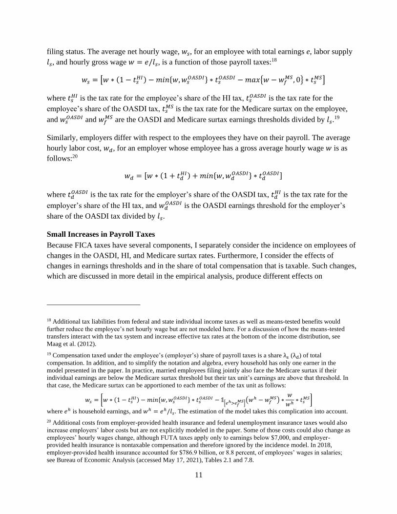
filing status. The average net hourly wage, 𝑤𝑠, for an employee with total earnings e, labor supply
𝑙𝑠, and hourly gross wage 𝑤 = 𝑒/𝑙𝑠, is a function of those payroll taxes:18
𝑤𝑠 = [𝑤 ∗ (1 − 𝑡𝑠𝐻𝐼) − 𝑚𝑖𝑛{𝑤,𝑤𝑠
𝑂𝐴𝑆𝐷𝐼} ∗ 𝑡𝑠𝑂𝐴𝑆𝐷𝐼 −𝑚𝑎𝑥{𝑤 − 𝑤𝑓
𝑀𝑆, 0} ∗ 𝑡𝑠𝑀𝑆]
where 𝑡𝑠𝐻𝐼 is the tax rate for the employee’s share of the HI tax, 𝑡𝑠
𝑂𝐴𝑆𝐷𝐼 is the tax rate for the
employee’s share of the OASDI tax, 𝑡𝑠𝑀𝑆 is the tax rate for the Medicare surtax on the employee,
and 𝑤𝑠𝑂𝐴𝑆𝐷𝐼 and 𝑤𝑓
𝑀𝑆 are the OASDI and Medicare surtax earnings thresholds divided by 𝑙𝑠.19
Similarly, employers differ with respect to the employees they have on their payroll. The average
hourly labor cost, 𝑤𝑑, for an employer whose employee has a gross average hourly wage 𝑤 is as
follows:20
𝑤𝑑 = [𝑤 ∗ (1 + 𝑡𝑑𝐻𝐼) + 𝑚𝑖𝑛{𝑤,𝑤𝑑
𝑂𝐴𝑆𝐷𝐼} ∗ 𝑡𝑑𝑂𝐴𝑆𝐷𝐼]
where 𝑡𝑑𝑂𝐴𝑆𝐷𝐼 is the tax rate for the employer’s share of the OASDI tax, 𝑡𝑑
𝐻𝐼 is the tax rate for the
employer’s share of the HI tax, and 𝑤𝑑𝑂𝐴𝑆𝐷𝐼 is the OASDI earnings threshold for the employer’s
share of the OASDI tax divided by 𝑙𝑠.
Small Increases in Payroll Taxes
Because FICA taxes have several components, I separately consider the incidence on employees of
changes in the OASDI, HI, and Medicare surtax rates. Furthermore, I consider the effects of
changes in earnings thresholds and in the share of total compensation that is taxable. Such changes,
which are discussed in more detail in the empirical analysis, produce different effects on
18 Additional tax liabilities from federal and state individual income taxes as well as means-tested benefits would
further reduce the employee’s net hourly wage but are not modeled here. For a discussion of how the means-tested
transfers interact with the tax system and increase effective tax rates at the bottom of the income distribution, see
Maag et al. (2012).
19 Compensation taxed under the employee’s (employer’s) share of payroll taxes is a share λs (λd) of total
compensation. In addition, and to simplify the notation and algebra, every household has only one earner in the
model presented in the paper. In practice, married employees filing jointly also face the Medicare surtax if their
individual earnings are below the Medicare surtax threshold but their tax unit’s earnings are above that threshold. In
that case, the Medicare surtax can be apportioned to each member of the tax unit as follows:
𝑤𝑠 = [𝑤 ∗ (1 − 𝑡𝑠𝐻𝐼) − 𝑚𝑖𝑛{𝑤,𝑤𝑠
𝑂𝐴𝑆𝐷𝐼} ∗ 𝑡𝑠𝑂𝐴𝑆𝐷𝐼 − 𝟙
[𝑒ℎ>𝑒𝑓𝑀𝑆](𝑤ℎ − 𝑤𝑓
𝑀𝑆) ∗𝑤
𝑤ℎ∗ 𝑡𝑠
𝑀𝑆]
where 𝑒ℎ is household earnings, and 𝑤ℎ = 𝑒ℎ/𝑙𝑠. The estimation of the model takes this complication into account.
20 Additional costs from employer-provided health insurance and federal unemployment insurance taxes would also
increase employers’ labor costs but are not explicitly modeled in the paper. Some of those costs could also change as
employees’ hourly wages change, although FUTA taxes apply only to earnings below $7,000, and employer-
provided health insurance is nontaxable compensation and therefore ignored by the incidence model. In 2018,
employer-provided health insurance accounted for $786.9 billion, or 8.8 percent, of employees’ wages in salaries;
see Bureau of Economic Analysis (accessed May 17, 2021), Tables 2.1 and 7.8.
12
employees’ net wages and employers’ labor costs. However, the formula used to compute the share
of the additional tax burden on employees affected is the same in each case:
𝑆𝐻𝐵𝑠 = −𝜀𝐷
𝜀𝑆 (1+𝐴𝑇𝑅𝑑1 − 𝐴𝑇𝑅𝑠
) − 𝜀𝐷
As in the simple model with proportional payroll taxes, the share of the burden on employees
affected by the change depends on labor demand elasticities, labor supply elasticities, and average
tax rates on employees and employers. In addition, this model predicts that the share of the burden
on employees does not depend on the statutory incidence of the tax, as in the simple model. In
contrast to the simple model, where income and substitution effects (and, therefore, labor supply
elasticities) are the same for every employee, those effects can differ by employee and further
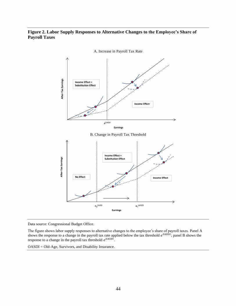
depend on the type of tax change considered.21 For example, an increase in the OASDI tax rate on
the employee, as shown in panel A of Figure 2, produces both income and substitution effects for
employees with earnings below the OASDI threshold but only income effects for employees above
that threshold. By contrast, an increase in the OASDI threshold produces both income and
substitution effects for employees with earnings between the old and the new thresholds but only
income effects for employees above the new threshold, as shown in panel B of Figure 2. As a result,
estimated labor supply elasticities differ among employees.
Average Share of the Tax Burden on Employees for Small Payroll Tax Changes
The formulas above provide the basis for estimating employees’ share of payroll tax changes.
Because marginal and average tax rates differ among employees and because labor supply
elasticities are also a function of those tax rates, the share of the burden differs for employees with
different earnings. In addition, the formulas apply only to employees who face a change in their
payroll tax liability.
If the share of the burden on employees is determined separately at each earnings level e because
wages are negotiated separately at each earnings level, the average share of the additional tax
burden falling on affected employees is a weighted average of those employees’ estimated burden at
each earning level, when taking into account the distribution of earnings of affected employees:
𝑆𝐻𝐵𝑠𝑑𝜏 = ∫ 𝑆𝐻𝐵𝑠
𝑒,𝑑𝜏(𝜀𝑆𝑒,𝑑𝜏 , 𝜀𝐷 , 𝐴𝑇𝑅𝑠
𝑒 , 𝐴𝑇𝑅𝑑𝑒)𝑓(𝑒)𝑑𝑒
𝑒𝑚𝑎𝑥
𝑒=0
where 𝑓(𝑒) is the earnings density function for employees affected by the change, and 𝑒𝑚𝑎𝑥 is the
highest observed earnings level. In this case, the average pass-through of a change in the
employee’s share of payroll taxes is a function of the employee’s gross earnings distribution but
21 A similar consideration applies to employers.
13
also depends on labor supply elasticities at each level of earnings (𝜀𝑆𝑒), the labor demand elasticity
(𝜀𝐷), the average tax rates (𝐴𝑇𝑅𝑠𝑒 , 𝐴𝑇𝑅𝑑
𝑒), and the type of payroll tax change 𝑑𝜏.22
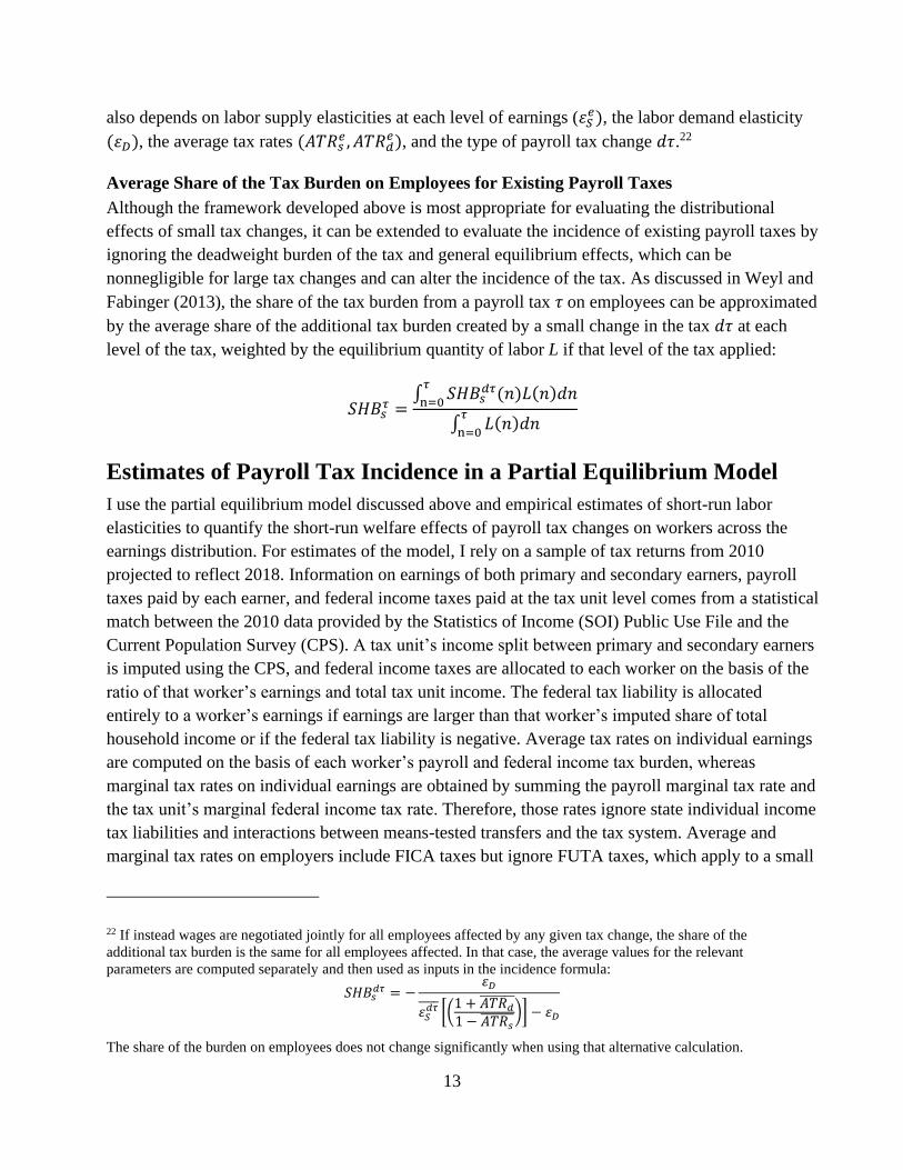
Average Share of the Tax Burden on Employees for Existing Payroll Taxes
Although the framework developed above is most appropriate for evaluating the distributional
effects of small tax changes, it can be extended to evaluate the incidence of existing payroll taxes by
ignoring the deadweight burden of the tax and general equilibrium effects, which can be
nonnegligible for large tax changes and can alter the incidence of the tax. As discussed in Weyl and
Fabinger (2013), the share of the tax burden from a payroll tax 𝜏 on employees can be approximated
by the average share of the additional tax burden created by a small change in the tax 𝑑𝜏 at each
level of the tax, weighted by the equilibrium quantity of labor L if that level of the tax applied:
𝑆𝐻𝐵𝑠𝜏 =
∫ 𝑆𝐻𝐵𝑠𝑑𝜏(𝑛)𝐿(𝑛)𝑑𝑛
𝜏
n=0
∫ 𝐿(𝑛)𝑑𝑛𝜏
n=0
Estimates of Payroll Tax Incidence in a Partial Equilibrium Model
I use the partial equilibrium model discussed above and empirical estimates of short-run labor
elasticities to quantify the short-run welfare effects of payroll tax changes on workers across the
earnings distribution. For estimates of the model, I rely on a sample of tax returns from 2010
projected to reflect 2018. Information on earnings of both primary and secondary earners, payroll
taxes paid by each earner, and federal income taxes paid at the tax unit level comes from a statistical
match between the 2010 data provided by the Statistics of Income (SOI) Public Use File and the
Current Population Survey (CPS). A tax unit’s income split between primary and secondary earners
is imputed using the CPS, and federal income taxes are allocated to each worker on the basis of the
ratio of that worker’s earnings and total tax unit income. The federal tax liability is allocated
entirely to a worker’s earnings if earnings are larger than that worker’s imputed share of total
household income or if the federal tax liability is negative. Average tax rates on individual earnings
are computed on the basis of each worker’s payroll and federal income tax burden, whereas
marginal tax rates on individual earnings are obtained by summing the payroll marginal tax rate and
the tax unit’s marginal federal income tax rate. Therefore, those rates ignore state individual income
tax liabilities and interactions between means-tested transfers and the tax system. Average and
marginal tax rates on employers include FICA taxes but ignore FUTA taxes, which apply to a small
22 If instead wages are negotiated jointly for all employees affected by any given tax change, the share of the
additional tax burden is the same for all employees affected. In that case, the average values for the relevant
parameters are computed separately and then used as inputs in the incidence formula:
𝑆𝐻𝐵𝑠𝑑𝜏 = −
𝜀𝐷
𝜀𝑆𝑑𝜏̅̅ ̅̅ [(
1 + 𝐴𝑇𝑅𝑑̅̅ ̅̅ ̅̅ ̅
1 − 𝐴𝑇𝑅𝑠̅̅ ̅̅ ̅̅ ̅)] − 𝜀𝐷
The share of the burden on employees does not change significantly when using that alternative calculation.
14
share of employees’ earnings, and employer-provided health insurance, which is currently
nontaxable and therefore ignored in the tax incidence model.23 In addition, I abstract from
differences in hours worked among workers because that information is not available from the SOI
data and compute hourly gross wages by assuming that each worker works 40 hours a week for
48 weeks a year.24 Worker are weighted by the weight that SOI assigns to their tax unit.
In this analysis, I focus on the tax burden of FICA taxes and use the tax parameters relevant for
2018. If a tax unit pays the Medicare surtax and has more than one earner, I apportion the Medicare
surtax to workers on the basis of their share of the tax unit’s total earnings. In addition, I use CBO’s
estimates of income and substitution effects to calculate labor supply elasticities at each earnings
level.25 As discussed below, those elasticities differ by earnings level partly because average and
marginal tax rates on earnings are different. Finally, I use estimates of labor demand elasticities
from Lichter et al. (2015), who survey the literature on own-wage demand elasticities estimated for
a large set of countries, including the United States.
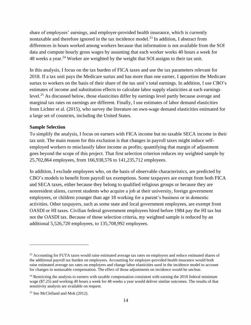
Sample Selection
To simplify the analysis, I focus on earners with FICA income but no taxable SECA income in their
tax unit. The main reason for this exclusion is that changes in payroll taxes might induce self-
employed workers to misclassify labor income as profits; quantifying that margin of adjustment
goes beyond the scope of this project. That first selection criterion reduces my weighted sample by
25,702,864 employees, from 166,938,576 to 141,235,712 employees.
In addition, I exclude employees who, on the basis of observable characteristics, are predicted by
CBO’s models to benefit from payroll tax exemptions. Some taxpayers are exempt from both FICA
and SECA taxes, either because they belong to qualified religious groups or because they are
nonresident aliens, current students who acquire a job at their university, foreign government
employees, or children younger than age 18 working for a parent’s business or in domestic
activities. Other taxpayers, such as some state and local government employees, are exempt from
OASDI or HI taxes. Civilian federal government employees hired before 1984 pay the HI tax but
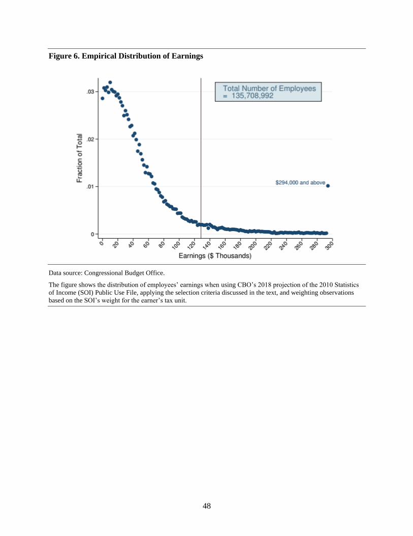
not the OASDI tax. Because of those selection criteria, my weighted sample is reduced by an
additional 5,526,720 employees, to 135,708,992 employees.
23 Accounting for FUTA taxes would raise estimated average tax rates on employers and reduce estimated shares of
the additional payroll tax burden on employees. Accounting for employer-provided health insurance would both
raise estimated average tax rates on employers and change labor elasticities used in the incidence model to account
for changes in nontaxable compensation. The effect of those adjustments on incidence would be unclear.
24 Restricting the analysis to earners with taxable compensation consistent with earning the 2018 federal minimum
wage ($7.25) and working 40 hours a week for 48 weeks a year would deliver similar outcomes. The results of that
sensitivity analysis are available on request.
25 See McClelland and Mok (2012).
15
Labor Supply Elasticities
When measured at a given point in time, labor supply elasticities include a substitution effect and an
income effect, both of which may alter people’s willingness to work. However, the substitution and
income effects generally have opposite outcomes. In the context of an increase in payroll taxes, the
substitution effect measures the decrease in an employee’s willingness to work following a
reduction in the after-tax compensation of an additional hour of work. The income effect measures
the increase in an employee’s willingness to work following a reduction in after-tax income for a
given amount of work. Both the income and substitution effects combine decisions about whether to
be employed and about how much labor to supply.
On the basis of a review of the literature, CBO estimates substitution and income effects for
permanent changes in income. CBO estimates an average midpoint substitution elasticity of 0.25 for
primary earners and 0.32 for secondary earners, as well as substitution elasticities by earnings decile
for primary earners. Specifically, the substitution elasticity is 0.31 for primary earners in the lowest
earnings decile, 0.28 for earners in the second lowest decile, 0.27 for earners in the third and fourth
deciles, 0.25 for earners in the fifth and sixth deciles, and 0.22 for earners in the top three deciles.
Because earnings of primary and secondary earners are imputed for each tax unit and because
primary earners can be split into earnings deciles, I apply those elasticities to the relevant workers in
my analysis. Unlike substitution elasticities, income elasticities do not differ among earners in
CBO’s estimates and range between -0.10 and zero for all earners. I use -0.05 as the midrange
income elasticity in my analysis. 26
One possible caveat of using substitution and income elasticities estimated in the literature is that
those were estimated with respect to changes in individual income taxes rather than changes in
payroll taxes. However, the adjustment necessary to account for that difference is unclear. On the
one hand, the empirical literature on other countries shows that labor supply can sometimes respond
more to income tax changes than to payroll tax changes.27 For example, to the extent that payroll
taxes are linked to higher Social Security benefits in retirement, people may be less responsive to
them than they are to income taxes. On the other hand, some recent studies show that average U.S.
federal income tax rates are often misperceived.28 That could potentially reduce labor supply
responses to changes in individual income taxes relative to changes in payroll taxes.
A second caveat, which relates to using average income elasticities to estimate the incidence of
payroll taxes on employees with different earnings, is that the actual elasticities might differ by
earnings. For example, if employees with low earnings have a lower (more negative) income
elasticity than employees with high earnings, then the framework defined below underestimates the
26 For a discussion of recent evidence on labor supply elasticities, see McClelland and Mok (2012).
27 For evidence on France, see Lehmann et al. (2013).
28 For example, see Slemrod (2006) and Ballard and Gupta (2018).
16
burden of a tax rate change on employees with low earnings and overestimates it for those with high
earnings.
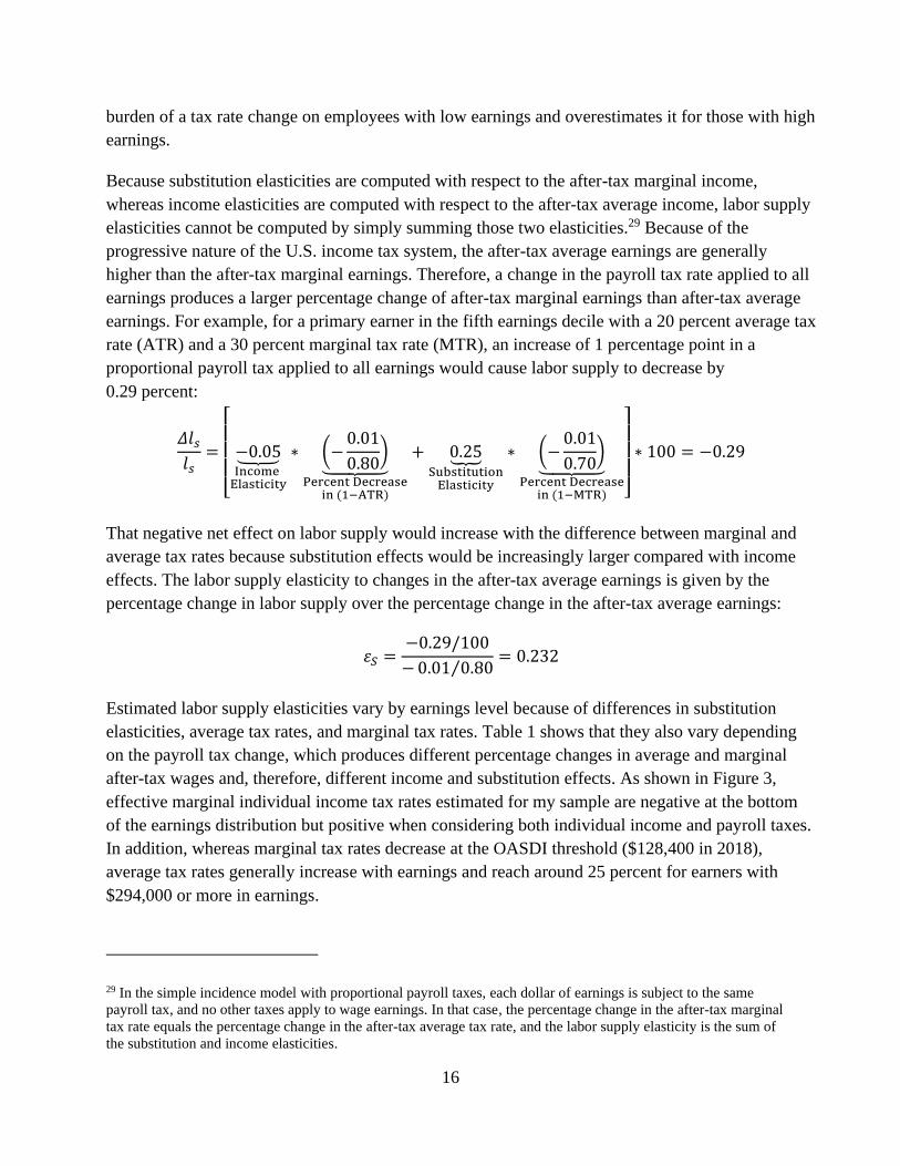
Because substitution elasticities are computed with respect to the after-tax marginal income,
whereas income elasticities are computed with respect to the after-tax average income, labor supply
elasticities cannot be computed by simply summing those two elasticities.29 Because of the
progressive nature of the U.S. income tax system, the after-tax average earnings are generally
higher than the after-tax marginal earnings. Therefore, a change in the payroll tax rate applied to all
earnings produces a larger percentage change of after-tax marginal earnings than after-tax average
earnings. For example, for a primary earner in the fifth earnings decile with a 20 percent average tax
rate (ATR) and a 30 percent marginal tax rate (MTR), an increase of 1 percentage point in a
proportional payroll tax applied to all earnings would cause labor supply to decrease by
0.29 percent:
𝛥𝑙𝑠𝑙𝑠=
[
−0.05⏟ Income Elasticity
∗ (−0.01
0.80)
⏟ Percent Decrease
in (1−ATR)
+ 0.25⏟SubstitutionElasticity
∗ (−0.01
0.70)
⏟ Percent Decreasein (1−MTR) ]
∗ 100 = −0.29
That negative net effect on labor supply would increase with the difference between marginal and
average tax rates because substitution effects would be increasingly larger compared with income
effects. The labor supply elasticity to changes in the after-tax average earnings is given by the
percentage change in labor supply over the percentage change in the after-tax average earnings:
𝜀𝑆 =−0.29/100
−0.01 0.80⁄= 0.232
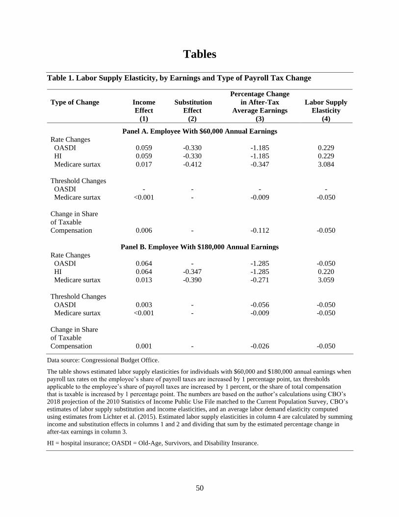
Estimated labor supply elasticities vary by earnings level because of differences in substitution
elasticities, average tax rates, and marginal tax rates. Table 1 shows that they also vary depending
on the payroll tax change, which produces different percentage changes in average and marginal
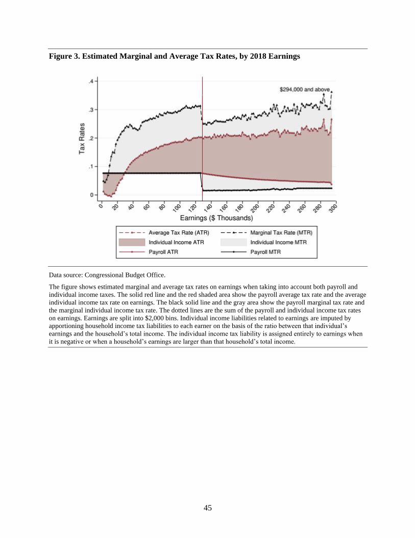
after-tax wages and, therefore, different income and substitution effects. As shown in Figure 3,
effective marginal individual income tax rates estimated for my sample are negative at the bottom
of the earnings distribution but positive when considering both individual income and payroll taxes.
In addition, whereas marginal tax rates decrease at the OASDI threshold ($128,400 in 2018),
average tax rates generally increase with earnings and reach around 25 percent for earners with
$294,000 or more in earnings.
29 In the simple incidence model with proportional payroll taxes, each dollar of earnings is subject to the same
payroll tax, and no other taxes apply to wage earnings. In that case, the percentage change in the after-tax marginal
tax rate equals the percentage change in the after-tax average tax rate, and the labor supply elasticity is the sum of
the substitution and income elasticities.
17
Labor Demand Elasticities
Own-wage demand elasticities—that is, the percentage change in employment in response to a
change in wages—include a scale effect and a substitution effect. Both of those effects determine a
firm’s willingness to change their decisions about how many workers to employ and for how many
hours each week.30 The scale effect measures the change in employment associated with a change in
wages, when holding the production technology constant and ignoring substitution between labor
and other inputs of production. The substitution effect measures the change in employment
associated with a change in wages, when holding total output constant (that is, ignoring the
additional resources available for purchasing labor and capital). Both of those effects are generally
believed to be negative, though estimates vary depending on the source of data used, the time
horizon over which the elasticity is estimated, and the country for which it is estimated. For
example, elasticity estimates obtained from firm-level data generally exceed estimates from
industry-level data, and labor demand is generally found to be less elastic in the short run than in the
long run.31
A recent literature review of 44 studies between 1971 and 2010 found that estimated own-wage
elasticities of labor demand in the United States averaged -0.43 in the short run. Because estimates
of labor demand elasticities are not available for workers of different earnings, that labor demand
elasticity is set to be the same for all workers.32 In practice, workers with different levels of earnings
or employed in different industries could face different labor demand elasticities, and nonlinearity
in the payroll tax schedule could generate some discontinuity in labor demand elasticities around
payroll tax thresholds.
Estimated Share of the Tax Burden on Employees for Small Payroll Tax Changes
The statutory incidence of payroll tax changes does not drive the predictions of the theoretical
model. For example, a change in the employer’s share of payroll taxes produces the same burden on
employees as a change in the employee’s share of payroll taxes. That is because those models do
not include features of the labor market that might be asymmetric. For example, the statutory
incidence might be important in the short run if there are fixed-term labor contracts. If so, an
increase in payroll taxes levied on the employer might produce a lower pass-through to employees
than an increase in payroll taxes levied on the employee.
30 The academic literature also focuses on cross-wage demand elasticities, which are elasticities of demand for
inputs of production when changing the price of other inputs of production.
31 For a recent meta-analysis of the literature on labor demand elasticities, see Lichter et al. (2015).
32 Accounting for the fact that labor demand elasticities for low-skill (and low-earnings) workers is higher than for
high-skill workers would, for example, further increase the incidence on those workers relative to the incidence on
high-skill workers. Because there is a higher density of workers at the bottom of the earnings distribution, the
average incidence on workers affected would also increase as a result.
18
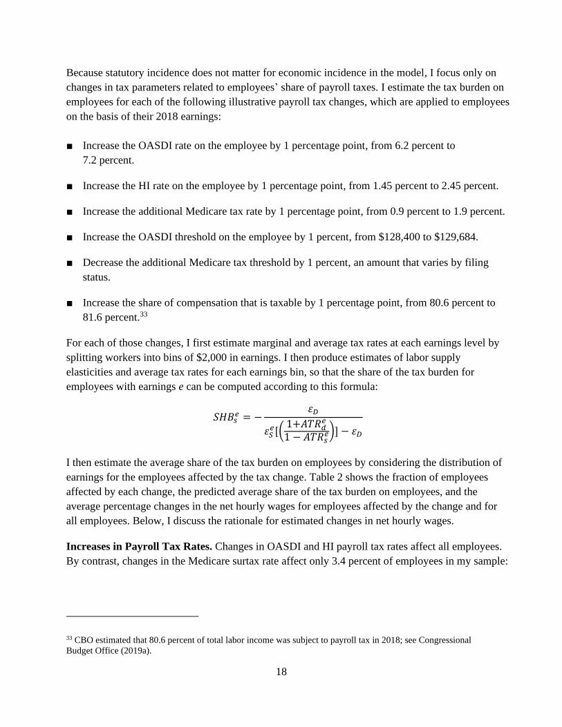
Because statutory incidence does not matter for economic incidence in the model, I focus only on
changes in tax parameters related to employees’ share of payroll taxes. I estimate the tax burden on
employees for each of the following illustrative payroll tax changes, which are applied to employees
on the basis of their 2018 earnings:
■ Increase the OASDI rate on the employee by 1 percentage point, from 6.2 percent to
7.2 percent.
■ Increase the HI rate on the employee by 1 percentage point, from 1.45 percent to 2.45 percent.
■ Increase the additional Medicare tax rate by 1 percentage point, from 0.9 percent to 1.9 percent.
■ Increase the OASDI threshold on the employee by 1 percent, from $128,400 to $129,684.
■ Decrease the additional Medicare tax threshold by 1 percent, an amount that varies by filing
status.
■ Increase the share of compensation that is taxable by 1 percentage point, from 80.6 percent to
81.6 percent.33
For each of those changes, I first estimate marginal and average tax rates at each earnings level by
splitting workers into bins of $2,000 in earnings. I then produce estimates of labor supply
elasticities and average tax rates for each earnings bin, so that the share of the tax burden for
employees with earnings e can be computed according to this formula:
𝑆𝐻𝐵𝑠𝑒 = −
𝜀𝐷
𝜀𝑆𝑒[(
1+𝐴𝑇𝑅𝑑𝑒
1 − 𝐴𝑇𝑅𝑠𝑒)] − 𝜀𝐷
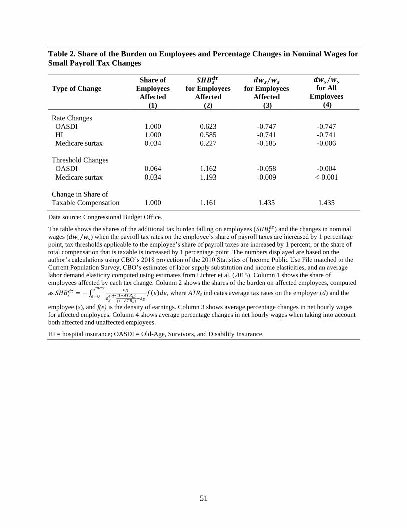
I then estimate the average share of the tax burden on employees by considering the distribution of
earnings for the employees affected by the tax change. Table 2 shows the fraction of employees
affected by each change, the predicted average share of the tax burden on employees, and the
average percentage changes in the net hourly wages for employees affected by the change and for
all employees. Below, I discuss the rationale for estimated changes in net hourly wages.
Increases in Payroll Tax Rates. Changes in OASDI and HI payroll tax rates affect all employees.
By contrast, changes in the Medicare surtax rate affect only 3.4 percent of employees in my sample:
33 CBO estimated that 80.6 percent of total labor income was subject to payroll tax in 2018; see Congressional
Budget Office (2019a).
19
those whose household earnings are above specified thresholds that vary by a household’s filing
status.
Increase in the Tax Rate for the Employee’s Share of the OASDI Tax. An increase of 1 percentage
point in the tax rate for the employee’s share of the OASDI tax produces differential effects for
employees below and above the OASDI threshold. It raises employees’ statutory payroll tax by
1 percent of gross wages for employees with gross wages below the OASDI threshold, therefore
increasing both their average and marginal tax rates. The estimated labor supply elasticity is
positive for those employees because their labor supply is predicted to decrease following a
reduction in their after-tax compensation. For those employees, the substitution effect, which
reduces their willingness to work, more than offsets their income effect, which increases their
willingness to work. By contrast, the tax change raises employees’ statutory payroll tax by 1 percent
of the OASDI threshold for employees with earnings above that threshold, therefore increasing their
average tax rates. Because the tax change has no effects on the marginal tax rates of those
employees and therefore produces no substitution effects, those employees’ labor supply increases
because of income effects. Their estimated labor supply elasticity is therefore negative. The change
in employees’ net hourly wages depends on their earnings, which determine their additional
statutory payroll tax liability and their average and marginal tax rates, as well as on estimated labor
elasticities:
𝑑𝑤𝑠𝑤𝑠
=min {𝑤,𝑤𝑠
𝑂𝐴𝑆𝐷𝐼}
𝑤(1 − 𝐴𝑇𝑅𝑠)
𝜀�̃�𝜀�̃� − 𝜀�̃�
where min {𝑤,𝑤𝑠𝑂𝐴𝑆𝐷𝐼} is the additional statutory payroll tax on employees, 𝜀�̃� and 𝜀�̃� are labor
supply and labor demand elasticities to changes in marginal after-tax wages and labor costs, and
𝐴𝑇𝑅𝑠 is the employee’s average tax rate on earnings. Specifically, 𝜀�̃� and 𝜀�̃� determine the fraction
of the additional tax burden shifted to employers. Panel A of Figure 4 shows that, because
employees below the OASDI threshold have increasing average tax rates, their percentage decrease
in after-tax wages is increasingly larger. The percentage reduction in after-tax wages for employees
whose earnings are just above the OASDI threshold is larger than for employees just below the
threshold because employees above the OASDI threshold increase their labor supply as payroll
taxes are raised. That effect is increasingly smaller as earnings increase because income effects
become smaller as earnings rise. Because estimated labor supply elasticities are positive below the
OASDI threshold and negative above that threshold, the share of the tax burden on employees is
about 60 percent in the first case and 120 percent in the second case, as shown in panel B of
Figure 4.
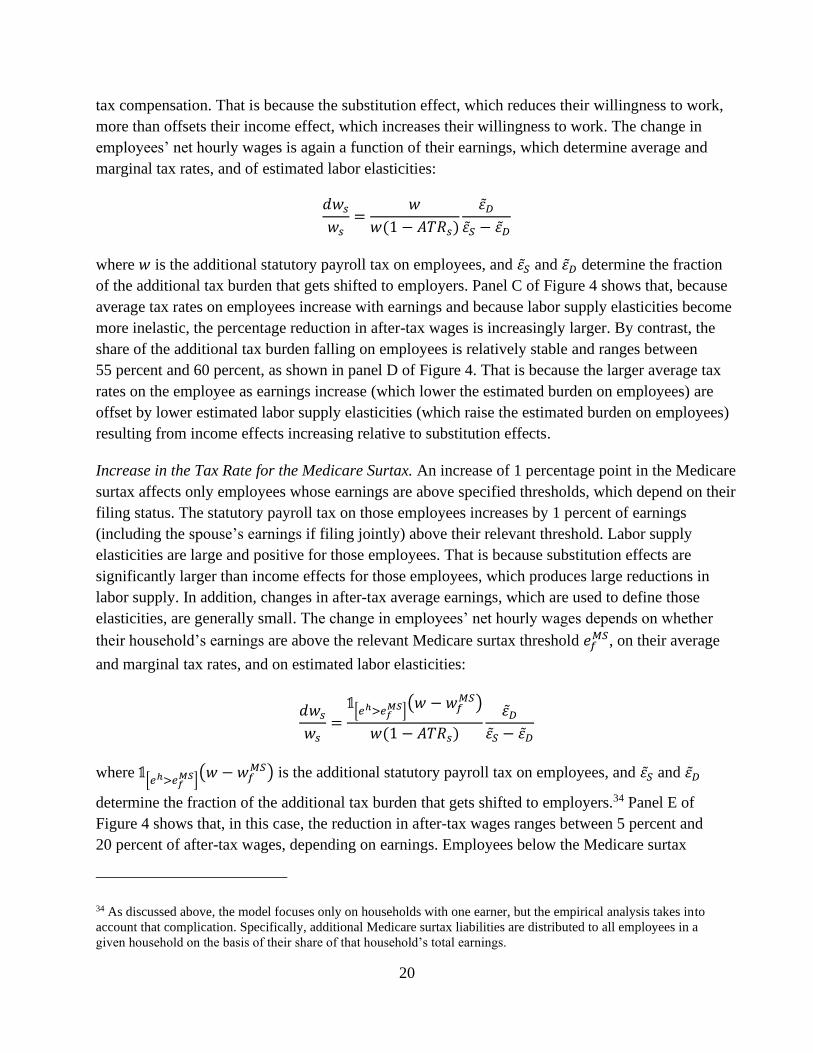
Increase in the Tax Rate for the Employee’s Share of the HI Tax. An increase of 1 percentage point
in the tax rate for the employee’s share of the HI tax raises employees’ statutory payroll tax by
1 percent of gross wages for all employees. The estimated labor supply elasticity is positive for all
employees because their labor supply is predicted to decrease following a reduction in their after-
20
tax compensation. That is because the substitution effect, which reduces their willingness to work,
more than offsets their income effect, which increases their willingness to work. The change in
employees’ net hourly wages is again a function of their earnings, which determine average and
marginal tax rates, and of estimated labor elasticities:
𝑑𝑤𝑠𝑤𝑠
=𝑤
𝑤(1 − 𝐴𝑇𝑅𝑠)
𝜀�̃�𝜀�̃� − 𝜀�̃�
where 𝑤 is the additional statutory payroll tax on employees, and 𝜀�̃� and 𝜀�̃� determine the fraction
of the additional tax burden that gets shifted to employers. Panel C of Figure 4 shows that, because
average tax rates on employees increase with earnings and because labor supply elasticities become
more inelastic, the percentage reduction in after-tax wages is increasingly larger. By contrast, the
share of the additional tax burden falling on employees is relatively stable and ranges between
55 percent and 60 percent, as shown in panel D of Figure 4. That is because the larger average tax
rates on the employee as earnings increase (which lower the estimated burden on employees) are
offset by lower estimated labor supply elasticities (which raise the estimated burden on employees)
resulting from income effects increasing relative to substitution effects.
Increase in the Tax Rate for the Medicare Surtax. An increase of 1 percentage point in the Medicare
surtax affects only employees whose earnings are above specified thresholds, which depend on their
filing status. The statutory payroll tax on those employees increases by 1 percent of earnings
(including the spouse’s earnings if filing jointly) above their relevant threshold. Labor supply
elasticities are large and positive for those employees. That is because substitution effects are
significantly larger than income effects for those employees, which produces large reductions in
labor supply. In addition, changes in after-tax average earnings, which are used to define those
elasticities, are generally small. The change in employees’ net hourly wages depends on whether
their household’s earnings are above the relevant Medicare surtax threshold 𝑒𝑓𝑀𝑆, on their average
and marginal tax rates, and on estimated labor elasticities:
𝑑𝑤𝑠𝑤𝑠
=𝟙[𝑒ℎ>𝑒𝑓
𝑀𝑆](𝑤 − 𝑤𝑓
𝑀𝑆)
𝑤(1 − 𝐴𝑇𝑅𝑠)
𝜀�̃�𝜀�̃� − 𝜀�̃�
where 𝟙[𝑒ℎ>𝑒𝑓
𝑀𝑆](𝑤 − 𝑤𝑓
𝑀𝑆) is the additional statutory payroll tax on employees, and 𝜀�̃� and 𝜀�̃�
determine the fraction of the additional tax burden that gets shifted to employers.34 Panel E of
Figure 4 shows that, in this case, the reduction in after-tax wages ranges between 5 percent and
20 percent of after-tax wages, depending on earnings. Employees below the Medicare surtax
34 As discussed above, the model focuses only on households with one earner, but the empirical analysis takes into
account that complication. Specifically, additional Medicare surtax liabilities are distributed to all employees in a
given household on the basis of their share of that household’s total earnings.
21
thresholds can also be affected if their household’s earnings are above the relevant Medicare surtax
threshold, and the percentage reduction in after-tax wages is larger for those employees because of
the higher income effect. The reduction in after-wages is increasingly larger as earnings rise
because income effects increase relative to substitution effects, leading to smaller reductions in
labor supply. That is shown in panel F of Figure 4: The share of the burden on employees generally
ranges between 10 percent and 20 percent but is about 40 percent for employees with earnings
above $300,000.
Changes in Payroll Tax Thresholds. Changes in tax thresholds affect only a subset of workers.
For example, if the OASDI tax threshold is increased to raise additional revenues, only workers
whose earnings are above the initial threshold (and their employers) are affected by the tax change.
If the Medicare surtax threshold is reduced to raise additional revenues, only workers whose
household earnings are above the new Medicare surtax threshold (and their employers) are affected
by the tax change. That accounts for 6.4 percent of employees in the first case and 3.4 percent of
employees in the second case.
Increase in the Threshold for the Employee’s Share of the OASDI Tax. A 1 percent increase in the
OASDI threshold for the employee’s share of the OASDI tax raises employees’ statutory payroll
taxes if the employee’s earnings are above the initial OASDI threshold. Specifically, employees
with earnings between the initial and the new OASDI thresholds face changes in both their average
and marginal tax rates on earnings, whereas employees with earnings above the new OASDI
thresholds experience changes only in their average tax rates on earnings. Therefore, I estimate that
labor supply decreases for the first group (because substitution effects more than offset income
effects) but increases for the second group (which experiences only income effects). The change in
employees’ net hourly wages depends on whether their earnings are above the initial OASDI
threshold 𝑒𝑂𝐴𝑆𝐷𝐼, on average and marginal tax rates, and on estimated labor elasticities:
𝑑𝑤𝑠𝑤𝑠
=𝟙[𝑒>𝑒𝑂𝐴𝑆𝐷𝐼]𝑡𝑠
𝑂𝐴𝑆𝐷𝐼
𝑤(1 − 𝐴𝑇𝑅𝑠)
𝜀�̃�𝜀�̃� − 𝜀�̃�
where 𝟙[𝑒>𝑒𝑂𝐴𝑆𝐷𝐼]𝑡𝑠𝑂𝐴𝑆𝐷𝐼 is the additional statutory payroll tax on employees, and 𝜀�̃� and 𝜀�̃�
determine the fraction of the additional tax burden that gets shifted to the employer. Panel A of
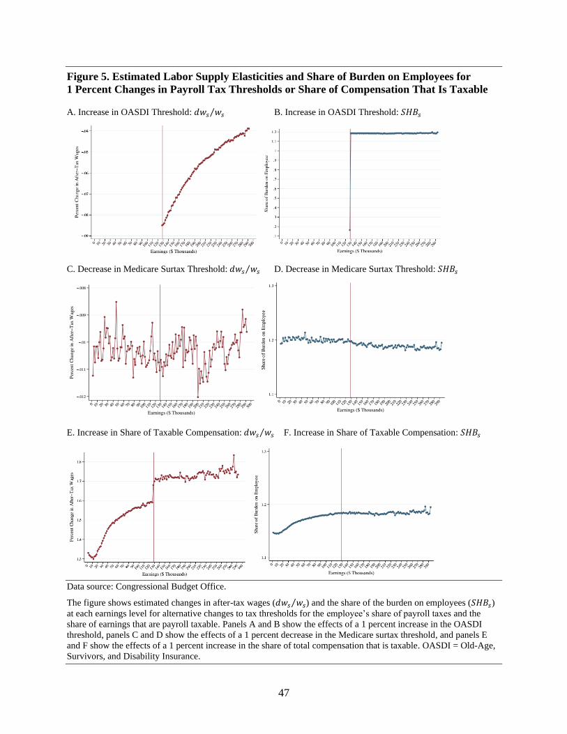
Figure 5 shows that the increase in the OASDI threshold affects only after-tax wages of employees
above the initial OASDI threshold. In addition, it shows that the percentage reduction in after-tax
wages is decreasing as earnings rise because income effects become increasingly smaller. Panel B
of Figure 5 also shows that, except for employees with earnings between the initial and new OASDI
threshold, whose share of the burden is low because of large and positive labor supply elasticities
(substitution effects are large relative to income effects in that case), the share of the burden for
most employees affected is about 120 percent of the total burden.
22
Decrease in the Medicare Surtax Threshold. A decrease in the Medicare surtax threshold raises
payroll taxes on employees with earnings above the new threshold, either because they were
previously untaxed or because more of their earnings are now taxed. Employees whose household
earnings are between the new and initial Medicare surtax thresholds face an increase in both
average and marginal tax rates on their earnings. By contrast, employees whose household earnings
are above the initial threshold face only an increase in their average tax rate on earnings. Therefore,
labor supply decreases for the first group because substitution effects more than offset income
effects but increases for the second group because of income effects. The change in employees’ net
hourly wages depends on whether their household’s earnings are above the relevant new Medicare
surtax threshold 𝑒𝑓𝑀𝑆, on average and marginal tax rates, and on estimated labor elasticities:
𝑑𝑤𝑠𝑤𝑠
=𝟙[𝑒ℎ>𝑒𝑓
𝑀𝑆]𝑡𝑠𝑀𝑆
𝑤(1 − 𝐴𝑇𝑅𝑠)
𝜀�̃�𝜀�̃� − 𝜀�̃�
where 𝟙[𝑒ℎ>𝑒𝑓
𝑀𝑆]𝑡𝑠𝑀𝑆 is the additional statutory payroll tax on employees, and 𝜀�̃� and 𝜀�̃� determine
the fraction of the additional tax burden that gets shifted to the employer. Panel C of Figure 5 shows
that the percentage decrease in after-tax wages is generally small and ranges between 0.08 percent
and 0.12 percent of after-tax wages. The estimated effects are generally largest right above existing
Medicare tax thresholds because income effects are largest in those cases but decrease as earnings
rise because income effects become increasingly small. The estimated share of the tax burden on
employees is about 120 percent because of negative labor supply elasticities and decreases with
earnings. That is because higher average tax rates on both employees and their employers more than
offset the reduction in labor supply elasticities.
Increase in Compensation That Is Taxed Under the Employee’s Share of Payroll Taxes. A
1 percent increase in the share of total compensation that is taxable under the employee’s share of
payroll taxes increases taxable compensation and payroll taxes for all employees, although it
reduces their total compensation. Employees whose earnings are below the OASDI threshold pay
additional OASDI and HI taxes on that previously untaxed compensation, whereas employees
whose earnings are above the OASDI threshold pay additional HI taxes. In addition, employees
whose household earnings are above the relevant Medicare surtax threshold pay additional
Medicare surtaxes. Labor supply increases because of income effects, which increase employees’
willingness to work after an increase in their after-tax taxable compensation. Labor supply
elasticities are therefore negative for all employees.
The change in compensation taxable under the employee’s share of payroll equals the sum of the
increase in after-tax wages resulting from the higher share of taxable compensation, net of the
decrease in taxable compensation negotiated by the employee to reduce the additional payroll tax
liability. As a result, the percentage increase in the employee’s after-tax wage is as follows:
23
𝑑𝑤𝑠𝑤𝑠
=−𝑤𝑡𝑜𝑡(1 − 𝑀𝑇𝑅𝑠)
𝑤(1 − 𝐴𝑇𝑅𝑠)
𝜀�̃�𝜆𝑑𝜀�̃�𝜆𝑠 − 𝜀�̃�𝜆𝑑
where 𝑤𝑡𝑜𝑡(1 −𝑀𝑇𝑅𝑠) is the additional statutory payroll tax on employees, 𝜆𝑠 and 𝜆𝑑 are the
shares of total compensation that are taxable under the employee’s and employer’s shares of payroll
taxes, and 𝜀�̃� and 𝜀�̃� determine the fraction of the additional tax burden that gets shifted to the
employer. Panel E of Figure 5 shows that the percentage increase in after-tax wages increases with
earnings, largely because of the increase in the average tax rates on the employee. Furthermore, the
percentage increase is significantly larger around the OASDI threshold, because newly taxable
earnings above the OASDI threshold face a significantly lower marginal tax rate (as shown in
Figure 3). The share of the tax burden on employees exceeds 100 percent for all employees because
of income effects, as shown in panel F of Figure 5.
Average Share of the Tax Burden on Employees. The average share of the tax burden on
employees is computed as a weighted average of the estimated shares of the tax burden on
employees at each earnings level. Figure 6 shows the density distribution used to compute that
average, and Table 2 shows those estimated average shares, as well as average percentage changes
in after-tax wages. I estimate that the additional tax burden of changes in payroll tax rates is split
between the employee and the employer. Small increases in OASDI and HI rates are associated
with an average share of the burden on employees of 62 percent and 58 percent, respectively, and
cause after-tax wages to decrease by about 0.74 percent. Instead, a small increase in the Medicare
surtax rate is associated with a 23 percent share of the burden on employees and a 0.18 percent
reduction in after-tax wages for employees affected by the change. By contrast, I estimate that
employees bear more than 100 percent of the additional burden created by changes in payroll tax
thresholds or in the share of total compensation that is taxable. That is because higher payroll taxes
increase employees’ willingness to work in such cases, which reduces gross wages. Therefore,
after-tax wages decrease both because of the higher payroll tax and because of the reduction in
gross wages. Unlike changes in the OASDI and the Medicare surtax thresholds, which affect a small
share of employees and reduce after-tax wages, an increase in the share of total compensation that is
taxable affects all employees and increases their after-tax wages, though it reduces their total
compensation. I estimate that employees’ after-tax wages decrease by less than 0.06 percent for
changes in thresholds but increase by 1.4 percent for an increase in the share of total compensation
that is taxable.
Estimated Share of the Tax Burden on Employees for Existing Payroll Taxes
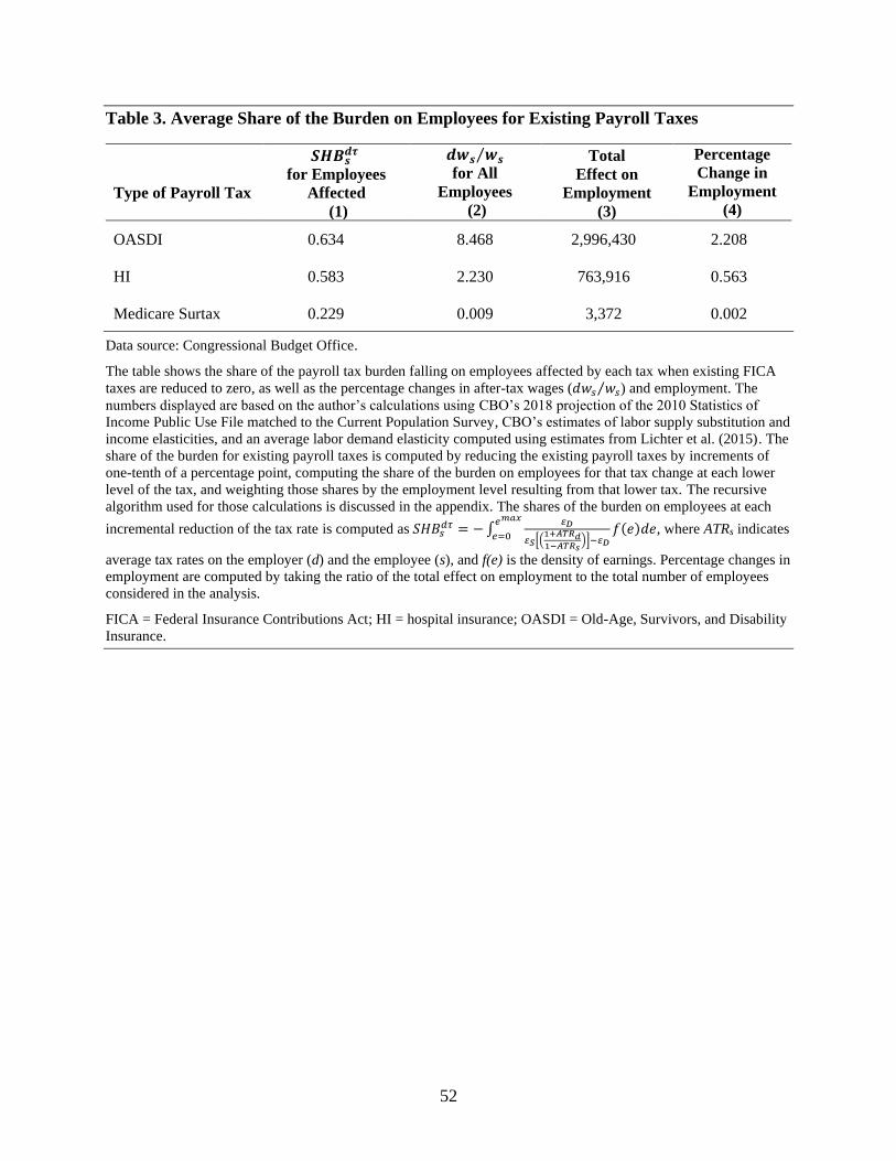
Figure 7 shows that the share of the tax burden on employees increases as payroll tax rates decline.
That is mainly because average tax rates on employees and employers also decrease as payroll taxes
are reduced. However, Table 3 shows that the estimated average share of the tax burden on
employees is not significantly different from that estimated for small tax changes. The total average
increase in employees’ after-tax wages ranges from 8.47 percent from OASDI taxes to
0.009 percent for the Medicare surtax. The change in total employment, which depends on changes
24
in nominal wages, ranges from 2.208 percent for OASDI taxes to 0.002 percent for the Medicare
surtax.
If taken at face value, those results suggest that nominal after-tax wages would increase by
10.7 percent when eliminating existing payroll taxes. Because the estimated average tax rate on
employees (which includes the employee’s share of payroll taxes and federal individual income
taxes) is 14.6 percent in my sample and because federal payroll taxes account for 15.3 percent of
earnings for most employees, eliminating existing payroll taxes would increase after-tax wages by
17.9 percent.35 Therefore, I estimate that employees bear 61.4 percent of the total payroll tax
burden.
General Equilibrium Effects of Payroll Tax Changes
Unlike partial equilibrium models, general equilibrium models take into account effects of tax
changes both in the market where the tax is imposed and in other markets, which might take longer
to adjust, and are therefore more suited for modeling the long-run incidence of tax changes.
However, because such models consider behavior in all markets, they also generally require a larger
set of parameter estimates, in addition to specifying how an increase in tax revenues is spent or how
a reduction in tax revenues is offset.
I use CBO’s overlapping generations model to examine the incidence of payroll tax changes on
employees in the long run when accounting for general equilibrium effects. In that model,
households decide how much labor to supply and how much disposable income to save in each
year, whereas firms use labor and productive capital as their only inputs of production and pay those
inputs their marginal products.36 Consistent with my partial equilibrium analysis, my incidence
analysis distinguishes between employees and employers. Specifically, employees are those who
supply labor, and employers are the owners of nonlabor factors of production, which include only
productive capital (but not land or nonland rents) in the OLG model.
As in the partial equilibrium model, I compute incidence from average changes in factor returns and
ignore other changes that could also affect the well-being of employees and employers.37 Therefore,
although my analysis provides a simple formula to estimate the share of the tax burden on
employees, it does not fully capture changes in consumption and the overall well-being of workers
35 The effect of eliminating existing payroll taxes on employees’ after-tax earnings is calculated as 15.3/(100 – 14.6)
= 0.179.
36 For a detailed description of that model, see Nishiyama (2003) and Congressional Budget Office (2019b).
37 For example, changes in interest income received on holdings of government debt and changes in future Social
Security benefits as payroll taxes are changed also affect the relative well-being of workers and owners of capital
but are ignored in the incidence analysis.
25
and owners of capital, which vary by age, income, and wealth.38 I estimate the share of the
additional payroll tax burden on employees using the ratio between the change in employees’ real
after-tax income and the overall change in real after-tax income when quantities of labor and capital
are kept fixed at their levels before the tax change: 39
𝑆𝐻𝐵𝐿 =
𝑑𝑤𝑤
𝑑𝑤𝑤 + 𝑘
𝑑𝑟𝑟
where 𝑑𝑤 𝑤⁄ is the percentage change in the average after-tax wage, 𝑑𝑟 𝑟⁄ is the percentage change
in the marginal product of capital, and k is the productive capital-to-labor ratio before the tax is
introduced. When a payroll tax is increased, employees bear less than the full burden of the tax if
both the after-tax wage and the marginal product of capital decrease. Instead, employees bear more
than the full burden of the tax if the after-tax wage decreases but the marginal product of capital
increases.
The percentage change in the average after-tax wage depends on changes in payroll tax liabilities
but also on changes in the before-tax wage. Unlike in the partial equilibrium analysis, income tax
liabilities also affect the after-tax wage. When considered in isolation, payroll tax increases would
reduce employees’ after-tax wage. The labor supply response to that reduction in the after-tax wage,
which depends on income and substitution effects but also on the Frisch elasticity, is also generally
negative in CBO’s OLG model.40 That reduction in labor supply contributes to increasing the
before-tax wage, with the effect of partially offsetting the reduction in the after-tax wage that results
from the higher payroll tax. The effect of the tax change on the before-tax wage would also depend
on how the revenues raised by a payroll tax change get used, as illustrated in Table 4. A reduction in
the capital stock, which I estimate when noninvestment government spending is increased to offset
a payroll tax increase, would make labor less productive, further reducing the before-tax wage. By
contrast, an increase in the capital stock, which I estimate when the additional revenues are used to
reduce government debt, would make labor more productive, increasing the before-tax wage and
offsetting some of the decrease in the after-tax wage.
The percentage change in the marginal product of capital would also depend on how the revenues
raised by a payroll tax increase get used, as illustrated in Table 4. For example, if the additional
38 For more information on the effect of payroll tax changes on households’ well-being by age, income, and wealth,
see Nelson and Phillips (2021).
39 For example, see Feldstein (1974) and the discussion of incidence in dynamic models in Fullerton and Metcalf
(2002). The denominator of the incidence formula approximates the fixed-quantities additional revenues collected
from the tax change.
40 The Frisch elasticity measures responses to a one-time, temporary change in after-tax compensation and equals
the sum of the substitution elasticity and a measure of people’s willingness to trade off work and consumption over
time. See Congressional Budget Office (2012) for a more detailed discussion of Frisch elasticities.
26
payroll tax revenues were used to increase noninvestment government spending and government
debt was held constant, both disposable income and private savings would be reduced. That would
reduce the capital stock and raise the marginal return on capital. By contrast, if those revenues were
used to reduce government debt, more household wealth would be invested in productive capital
despite the decrease in private savings. That would increase the capital stock and reduce the
marginal product of capital.
To compare the incidence of alternative hypothetical payroll tax changes on employees, I then
estimate the effects of alternative payroll tax changes when the tax revenues are used to increase (or
reduce) noninvestment government spending. Those estimates are presented in Table 5.41 The
effects of small increases in payroll taxes are shown in panel A. Small increases in payroll taxes
would reduce the average after-tax wage, and that reduction would be largest for increases in the
OASDI and HI tax rates. Those changes would affect all employees and reduce their average after-
tax wage by 1.07 percent in the first case and by 1.08 percent in the second case. A 1 percent
increase in the share of total compensation that is taxable would reduce the after-tax wage by
0.56 percent. The other changes considered in Table 5 would have limited effects on the average
after-tax wage. If the revenues were used to raise noninvestment government spending, payroll tax
increases would also reduce the stock of capital, therefore raising the marginal product of capital.
As a result, employees would bear more than the full burden of the tax in such cases, as shown in
column 3. The share of the burden on employees would range from 133 percent for an increase in
the OASDI tax rate to 145 percent for changes in the share of total compensation that is taxable.
The estimated effects of removing existing payroll taxes are displayed in panel B of Table 5.
Removing existing OASDI taxes would raise the average after-tax wage by 13.82 percent, and
removing existing HI taxes would raise it by 3.39 percent, with estimated reductions in the marginal
product of capital in each case. The percentage increase in the average after-tax wage from
removing the HI surtax would also be positive but small. Because the marginal product of capital
would decrease in all cases when the loss in payroll tax revenues is used to reduce noninvestment
government spending, the estimated incidence on employees in such cases would range from
141 percent for the OASDI tax to 151 percent for the HI tax.
41 The estimates for the 1 percentage-point increase in the HI tax rate when using the revenues to increase
noninvestment government spending differ in Table 4 and Table 5 because of the different setup. Table 4 shows the
long-run steady state following a transition path that follows the debt-to-GDP ratio published in CBO (2020b)
through 2030, after which debt is held constant through a closure rule. By contrast, government debt is held constant
from the year the tax policy is implemented in the estimate presented in Table 5. Therefore, the debt-to-GDP ratio is
higher in the steady state captured in Table 4 than it is in Table 5. That has the effects of reducing private savings
invested in productive capital, raising the marginal product of capital, and reducing workers’ after-tax wages.
27
Additional Insights From Recent Studies on Payroll Tax Incidence
Evidence on the incidence of payroll tax changes enacted at the national level in other countries,
mainly in Europe and South America, is mixed but often inconsistent with full pass-through of
payroll taxes to employees.42 Those studies provide estimates that are not directly applicable to the
United States because of the different institutional settings, but they offer insights that can help the
analysis of payroll tax incidence in the United States. Some of the mechanisms highlighted in that
work are not considered in the model of tax incidence developed above, which relies largely on
labor supply and labor demand elasticities and can therefore complement that analysis. For
example, those recent studies show that downward wage rigidity, the design and remittance of the
tax, the perceived linkage between current contributions and future benefits, the degree of firms’
market power, the state of the economy, and the institutional setting in which the tax is
implemented are all important determinants of payroll tax incidence.
Downward Wage Rigidity
Evidence from other countries shows that downward wage rigidities, some of which result from
minimum wage laws, are relevant for payroll tax incidence. Kugler and Kugler (2009) analyzed a
payroll tax change for Colombian manufacturing plants in the 1980s and 1990s and found lower
pass-through to hourly wages but larger employment effects for workers where minimum wages
were binding. Similarly, Saez et al. (2012a) focused on a cohort-based payroll tax reform in Greece
and showed significant downward rigidity in wages. They found that changes in the employer’s
share of the tax was generally borne by the employer because of downward wage rigidities, whereas
changes in the employee’s share of the tax was generally borne by the employee. In that context,
pay-fairness norms, wage-setting norms, and wage-bargaining norms all contributed to downward
wage rigidities. Other studies have emphasized the importance of the centralized wage bargaining
process and the frequency of wage negotiations as additional sources of downward wage rigidity.43
Wage rigidity is probably higher in countries with strong wage-setting norms and unionized
bargaining, but it also matters for the United States. Recent studies have found significant evidence
of downward wage rigidity in the United States.44 Because of that, the pass-through of increases in
the employer’s share of payroll taxes to wages is possibly more limited than the pass-through of the
employee’s share of payroll taxes, which does not require any adjustment in gross hourly wages for
the tax burden to fall on employees.
42 Melguizo and González-Páramo (2013) conducted a meta-analysis of the existing empirical literature on the
economic incidence of labor taxes and social security contributions and found that, on average, the incidence of
labor taxes on employees was 43 percent in the short run and 74 percent in the long run.
43 For the importance of centralized wage bargaining, see, for example, Bennmarker et al. (2009), Korkeamäki and
Uusitalo (2009), and Saez et al. (2019).
44 For a review of that literature, see Fallick et al. (2020).
28
Design and Remittance of the Tax
Previous studies have pointed out that the way a tax is designed and remitted is relevant for its
incidence. For example, Anderson and Meyer (2000) and Murphy (2007) discussed the effects of
transitioning from a uniform to an experience-based unemployment insurance (UI) payroll tax and
show that the reform reduced UI claims, stabilized employment, and reduced wages and salaries.
The higher burden on employers when firing workers shifted the incidence of the tax from
employment to wages. The way the tax is remitted also matters for the incidence of the tax. For
example, Slemrod (2008) focused on opportunities for tax avoidance and evasion linked to the
remittance system. Although employers withhold their employees’ Social Security payroll taxes, no
withholding is required for independent contractors, who are responsible for remitting payroll
taxes.45 Eliminating such withholding by the employer probably facilitates tax evasion and reduces
the pass-through of the tax to earnings of independent contractors. Because FICA, FUTA, and
SECA taxes have different designs and remittance systems, their incidence on earnings may also
differ.
Perceived Future Benefits
Previous research has shown that the pass-through to employees is generally higher when there is a
closer perceived link between payroll taxes paid and future Social Security benefits. Studies on
other countries highlight the tax-benefit linkage as an important determinant of payroll tax
incidence. For example, Kugler and Kugler (2009) studied the effects of a 1993 reform of the social
security system in Colombia and the corresponding increase in both payroll taxes and the overall
tax-benefit linkage. They found that the reform was associated with an increase in the pass-through
of payroll taxes to wages. Similarly, Bozio et al. (2019) studied three large increases in employer
social security contributions in France over the period 1976–2010 and found that shifting of the tax
to employees was related to the strength of the tax-benefit linkage.
The relevance of that tax-benefit linkage in the United States has been emphasized in the context of
mandated employer-provided benefits, which, like payroll taxes, are sometimes viewed as benefit
taxes.46 For example, Gruber (1994) showed that requiring employers to provide maternity benefits
in the United States in the 1970s produced a reduction in wages for women of childbearing age,
consistent with employees’ valuing those benefits. Lahey (2012) found that state mandates requiring
employer-provided health insurance plans to cover infertility treatment produced small effects on
wages, suggesting that employees did not value such benefits. Because the tax benefit-linkage for
FICA and SECA taxes varies according to the level of lifetime earnings, which are the base for
45 The employer is, however, required to file an information return for all annual payments above $600 unless the
contractor is a corporation.
46 However, the parallel between payroll tax changes and changes in employer-mandated benefits is not perfect. For
example, Summers (1989) argued that the incidence of payroll taxes and mandated benefits are different in that the
labor supply curve is shifting if employees value the benefits offered to them, whereas the labor supply curve never
shifts in the case of a payroll tax on the employer.
29
calculating Social Security benefits, it is possible that the incidence of the tax also varies across the
earnings distribution.
Degree of Firms’ Market Power
The incidence of payroll tax cuts on employees is probably higher in markets where firms have a
high bargaining power, and overshifting of the tax, which is a change in net hourly wage that is
larger than the change in the tax applied to that wage, is possible under some conditions.47 In those
markets, firms can set prices to maximize their profits. As a result, the pass-through of the tax to
employees also depends on the curvature of the labor demand function. Recent empirical work
shows that the degree of firms’ market power in U.S. labor markets depends on the particular
geographical area and industry considered and that a higher degree of firm concentration is
generally associated with lower wages.48 Though that effect is challenging to incorporate into the
incidence framework defined above because labor demand functions are unobservable, higher firm
concentration would probably increase the pass-through of payroll tax changes to employees.
State of the Economy
Previous work has emphasized the level of an economy’s structural unemployment as an important
determinant of labor supply and labor demand elasticities. Recent evidence on labor supply
elasticities over the business cycle is mixed. Some studies show that labor supply elasticities are
lower during economic downturns, in part because wages and outside employment options also
decrease during those times. Other studies show that labor supply elasticities increase during
recessions, possibly because households suffering from decreases in wealth become more
responsive to changes in wages.49 Evidence on the relationship between labor demand elasticities
and the state of the economy is more limited. Because the previous literature has provided
competing explanations of the relation between the state of the economy and labor elasticities,
which could move in one direction or the other, it is challenging to incorporate that relation into the
standard model.
Institutional Setting
The institutional setting is also an important determinant of payroll tax incidence. For example,
differences in social and wage-setting norms can contribute to explaining differences in payroll tax
incidence by country. Saez et al. (2012a) emphasized that pay-fairness, wage-setting, and wage-
bargaining norms are important determinants of payroll tax incidence in Greece. Similarly, Cruces
et al. (2010) focused on payroll tax incidence in Argentina and emphasized features of the labor
market specific to that country. They emphasized transaction costs, which are generally higher in
47 For a review of incidence in markets with imperfect competition, see Weyl and Fabinger (2013).
48 For a detailed discussion, see Azar et al. (2020).
49 For example, Depew and Sorensen (2013) showed that labor supply elasticities are lower during recessions. By
contrast, Attanasio et al. (2018) showed that labor supply elasticities are generally larger during recessions.
30
developing than in developed countries; geographic concentration of employment opportunities,
which affects labor supply elasticities; and the presence of minimum wage policies. Because of
differences in the institutional setting, results from other countries are often not applicable to the
United States.
Conclusion
Quantifying the incidence of U.S. federal payroll tax changes on employees is challenging because
there have been no recent permanent changes in federal payroll taxes in the United States. However,
theoretical models and empirical evidence on the effects of payroll tax changes in other countries
can inform analyses of the welfare effects of such payroll tax changes and help distinguish between
short-run and long-run incidence of those tax changes.
In this paper, I first developed a partial equilibrium model and used short-run labor elasticities to
estimate the short-run incidence of changes in FICA taxes. I showed that incidence estimates would
vary among hypothetical payroll tax changes. Specifically, I found that changes in payroll tax rates
would be associated with less than the full burden on employees. I estimated that 58 percent of the
additional short-run tax burden created by an increase in the HI tax rate, which applies
proportionally to all taxable compensation, would be on employees. The predicted additional tax
burden on employees for other changes in payroll tax rates varies: I estimated that 23 percent of the
tax burden from an increase in the additional Medicare surtax rate and 62 percent of the tax burden
from an increase in the OASDI tax rate would be shifted to employees in the short run. Instead,
changes in payroll tax thresholds or in the share of total compensation that is taxable would be
associated with more than full pass-through of the tax to employees. Using that same partial
equilibrium model, I estimated that 61.4 percent of the short-run benefit of eliminating all existing
FICA taxes would go to employees.
I then used CBO’s overlapping generations model to estimate the long-run general equilibrium
effects of changing those taxes. The incidence of payroll tax changes on employees, which I
estimated from changes in employees’ after-tax wage and the marginal product of capital, would
depend largely on the macroeconomic effects of those tax changes. How the payroll tax revenues
are used would affect those macroeconomic changes. For example, I estimated that employees
would bear more of the full burden of a proportional payroll tax increase if the revenues were used
to increase noninvestment government spending but would bear less than the full burden of that
proportional payroll tax increase if the revenues were used to reduce government debt. That is
because, although employees’ after-tax wages would decrease in both cases, the marginal return on
capital would increase in the first case but decrease in the second case. I then discussed the effects
of alternative hypothetical FICA tax changes when payroll tax changes are used for noninvestment
government spending.
Finally, I reviewed the existing literature on payroll tax incidence. That literature focuses largely on
other countries but is a useful complement to the model-based estimates presented in this paper. On
31
the one hand, it provides results that are consistent with my model-based estimates for the short run,
showing that employees generally bear less than the full burden of changes in payroll taxes. On the
other hand, it offers useful insights on the additional determinants of tax incidence, which are not
accounted for in my model-based estimates. For example, that literature suggests that both statutory
incidence and the direction of the tax change can matter for incidence. Therefore, the insights from
that literature caution against using the model-based estimates of this paper without accounting for
the specific features of the payroll tax change being implemented. That literature also offers useful
guidance for determining the incidence of future federal payroll tax changes implemented in the
United States.
32
Appendix
This appendix provides technical information about the derivation of incidence formulas with
proportional payroll taxes and with a nonlinear payroll tax schedule, as well as the recursive
algorithm used to compute the share of the tax burden for existing taxes.
Derivation of Incidence Formulas With Proportional Payroll Taxes
The derivations for the share of the burden on the employee for a small increase in a proportional
payroll tax on the employer or on the employee are presented below. In this simple model:
𝑤𝑠 = 𝑤(1 − 𝑡𝑠)
𝑤𝑑 = 𝑤(1 + 𝑡𝑑)
Change in the Employer’s Share of the Payroll Tax. Let 𝑡𝑑 be a proportional payroll tax on
the employer and 𝑑𝑡𝑑 be a small change in that tax rate. Then:
𝐷′(𝑤(1 + 𝑡𝑑))[𝑑𝑤
𝑑𝑡𝑑(1 + 𝑡𝑑) + 𝑤] = 𝑆′(𝑤(1 − 𝑡𝑠))
𝑑𝑤
𝑑𝑡𝑑(1 − 𝑡𝑠)
𝑑𝑤
𝑑𝑡𝑑[𝑆′(1 − 𝑡𝑠) − (1 + 𝑡𝑑)𝐷
′] = 𝑤𝐷′
Because 𝜀𝐷 =𝐷′
𝐿𝑤(1 + 𝑡𝑑) and 𝜀𝑆 =
𝑆′
𝐿𝑤(1 − 𝑡𝑠), we get that:
𝑑𝑤
𝑑𝑡𝑑=
𝑤
(1 + 𝑡𝑑)
𝜀𝐷(𝜀𝑆 − 𝜀𝐷)
It follows that: 𝑑𝑤𝑑𝑑𝑡𝑑
=𝑑𝑤
𝑑𝑡𝑑(1 + 𝑡𝑑) + 𝑤 = 𝑤
𝜀𝑆(𝜀𝑆 − 𝜀𝐷)
and:
𝑑𝑤𝑠𝑑𝑡𝑑
=𝑑𝑤
𝑑𝑡𝑑(1 − 𝑡𝑠) = 𝑤
(1 − 𝑡𝑠)
(1 + 𝑡𝑑)
𝜀𝐷(𝜀𝑆 − 𝜀𝐷)
The tax revenues raised when holding all quantities fixed but allowing prices to vary are:
𝑑𝑅
𝑑𝑡𝑑= 𝑤 + (𝑡𝑠 + 𝑡𝑑)
𝑑𝑤
𝑑𝑡𝑑
33
Therefore, the share of the tax burden on employees is:
𝑆𝐻𝐵𝑠 = −
𝑑𝑤𝑠𝑑𝑡𝑑𝑑𝑅𝑑𝑡𝑑
= −𝜀𝐷
𝜀𝑆 (1+𝑡𝑑1 − 𝑡𝑠
) − 𝜀𝐷
This formula simplifies to −𝜀𝐷
(𝜀𝑆−𝜀𝐷) if there is no existing payroll tax, that is, if 𝑡𝑠 = 𝑡𝑑 = 0.
Change in the Employee’s Share of the Payroll Tax. Let 𝑡𝑠 be a proportional payroll tax on
the employee and 𝑑𝑡𝑠 be a small change in that tax rate. Then:
𝐷′(𝑤(1 + 𝑡𝑑))𝑑𝑤
𝑑𝑡𝑠(1 + 𝑡𝑑) = 𝑆′(𝑤(1 − 𝑡𝑠))[
𝑑𝑤
𝑑𝑡𝑠(1 − 𝑡𝑠) − 𝑤]
𝑑𝑤
𝑑𝑡𝑠[𝑆′(1 − 𝑡𝑠) − 𝐷
′(1 + 𝑡𝑑)] = 𝑤𝑆′
Because 𝜀𝐷 =𝐷′
𝐿𝑤(1 + 𝑡𝑑) and 𝜀𝑆 =
𝑆′
𝐿𝑤(1 − 𝑡𝑠), we get that:
𝑑𝑤
𝑑𝑡𝑠=
𝑤
(1 − 𝑡𝑠)
𝜀𝑆(𝜀𝑆 − 𝜀𝐷)
It follows that:
𝑑𝑤𝑑𝑑𝑡𝑠
=𝑑𝑤
𝑑𝑡𝑠(1 + 𝑡𝑑) = 𝑤
(1 + 𝑡𝑑)
(1 − 𝑡𝑠)
𝜀𝑆(𝜀𝑆 − 𝜀𝐷)
and:
𝑑𝑤𝑠𝑑𝑡𝑠
=𝑑𝑤
𝑑𝑡𝑠(1 − 𝑡𝑠) − 𝑤 = 𝑤
𝜀𝐷(𝜀𝑆 − 𝜀𝐷)
The tax revenues raised when holding all quantities fixed but allowing prices to vary are:
𝑑𝑅
𝑑𝑡𝑠= 𝑤 + (𝑡𝑠 + 𝑡𝑑)
𝑑𝑤
𝑑𝑡𝑠
Therefore, the share of the tax burden on employees is:
𝑆𝐻𝐵𝑠 = −
𝑑𝑤𝑠𝑑𝑡𝑠𝑑𝑅𝑑𝑡𝑠
= −𝜀𝐷
𝜀𝑆 (1+𝑡𝑑1 − 𝑡𝑠
) − 𝜀𝐷
34
This formula simplifies to −𝜀𝐷
(𝜀𝑆−𝜀𝐷) if there is no existing payroll tax, that is, if 𝑡𝑠 = 𝑡𝑑 = 0.
Derivation of Incidence Formulas With Nonlinear Payroll Taxes
An employee with gross earnings 𝑒 and labor supply 𝑙𝑠 earns gross hourly wage w and net hourly
wage 𝑤𝑠, and the worker’s employer has hourly labor costs 𝑤𝑑. If the employee is the only
earner in the household (𝑒ℎ = 𝑒):
𝑤𝑠 = [𝑒(1 − 𝑡𝑠𝐻𝐼) − 𝑚𝑖𝑛{𝑒, 𝑒𝑠
𝑂𝐴𝑆𝐷𝐼}𝑡𝑠𝑂𝐴𝑆𝐷𝐼 −𝑚𝑎𝑥{𝑒 − 𝑒𝑓
𝑀𝑆, 0} 𝑡𝑠𝑀𝑆] 𝑙𝑠⁄
𝑤𝑑 = [𝑒(1 + 𝑡𝑑𝐻𝐼) + 𝑚𝑖𝑛{𝑒, 𝑒𝑑
𝑂𝐴𝑆𝐷𝐼}𝑡𝑑𝑂𝐴𝑆𝐷𝐼] 𝑙𝑑⁄
where 𝑡𝑠𝑂𝐴𝑆𝐷𝐼 and 𝑡𝑑
𝑂𝐴𝑆𝐷𝐼 are the employee’s and employer’s share of the Old-Age, Survivors,
and Disability Insurance (OASDI) tax, 𝑡𝑠𝐻𝐼 and 𝑡𝑑
𝐻𝐼 are the employee’s and employer’s share of
the hospital insurance (HI) tax, 𝑡𝑠𝑀𝑆 is the Medicare surtax on the employee, and taxable income
thresholds 𝑒𝑂𝐴𝑆𝐷𝐼 and 𝑒𝑀𝑆 are OASDI and Medicare surtax thresholds. Define w = e/l,
𝑤𝑂𝐴𝑆𝐷𝐼 = 𝑒𝑂𝐴𝑆𝐷𝐼/𝑙, and 𝑤𝑓𝑀𝑆 = 𝑒𝑓
𝑀𝑆/𝑙, and let 𝑒ℎ denote household earnings. For simplicity and
without loss of generality, I impose the same threshold for the employer’s and employee’s share
of payroll taxes when changing tax rates (𝑒𝑠𝑂𝐴𝑆𝐷𝐼 = 𝑒𝑑
𝑂𝐴𝑆𝐷𝐼 = 𝑒𝑂𝐴𝑆𝐷𝐼).
Finally, 𝜀𝑆 denotes the employee’s labor supply elasticity with respect to percentage changes in
the average after-tax wage, and 𝜀𝐷 denotes the employer’s labor demand elasticity with respect
to percentage changes in the average labor cost. Instead, 𝜀�̃� = 𝜀𝑆𝑤(1−𝑀𝑇𝑅𝑠)
𝑤(1−𝐴𝑇𝑅𝑠) and 𝜀�̃� =
𝜀𝐷𝑤(1+𝑀𝑇𝑅𝑑)
𝑤(1+𝐴𝑇𝑅𝑑) are labor elasticities expressed in terms of percentage changes in the marginal
employee’s after-tax wage and employer’s labor cost.
Change in the OASDI Tax Rate for the Employer’s Share of OASDI. Let 𝑡𝑑𝑂𝐴𝑆𝐷𝐼 be the
OASDI tax rate for the employer’s share of the OASDI tax and 𝑑𝑡𝑑𝑂𝐴𝑆𝐷𝐼 be a small change in that
tax rate. Then:
𝑑𝑤
𝑑𝑡𝑑𝑂𝐴𝑆𝐷𝐼
(𝑒) =
{
𝑤
𝜀𝐷
𝜀𝑆(1 − 𝑡𝑠𝐻𝐼 − 𝑡𝑠
𝑂𝐴𝑆𝐷𝐼)𝑤𝑑𝑤𝑠
− 𝜀𝐷(1 + 𝑡𝑑𝐻𝐼 + 𝑡𝑑
𝑂𝐴𝑆𝐷𝐼)
𝑖𝑓 𝑒 ≤ 𝑒𝑂𝐴𝑆𝐷𝐼
𝑤𝑂𝐴𝑆𝐷𝐼𝜀𝐷
𝜀𝑆(1 − 𝑡𝑠𝐻𝐼)𝑤𝑑
𝑤𝑠− 𝜀𝐷(1 + 𝑡𝑑
𝐻𝐼) 𝑖𝑓 𝑒 > 𝑒𝑂𝐴𝑆𝐷𝐼 , 𝑒ℎ ≤ 𝑒𝑓
𝑀𝑆
𝑤𝑂𝐴𝑆𝐷𝐼𝜀𝐷
𝜀𝑆(1 − 𝑡𝑠𝐻𝐼 − 𝑡𝑠
𝑀𝑆)𝑤𝑑𝑤𝑠
− 𝜀𝐷(1 + 𝑡𝑑𝐻𝐼)
𝑖𝑓 𝑒 > 𝑒𝑂𝐴𝑆𝐷𝐼 , 𝑒ℎ > 𝑒𝑓𝑀𝑆
35
Define:
𝑀𝑇𝑅𝑑(𝑒) = {(𝑡𝑑𝐻𝐼 + 𝑡𝑑
𝑂𝐴𝑆𝐷𝐼) 𝑖𝑓 𝑒 ≤ 𝑒𝑂𝐴𝑆𝐷𝐼
𝑡𝑑𝐻𝐼 𝑖𝑓 𝑒 > 𝑒𝑂𝐴𝑆𝐷𝐼
𝑀𝑇𝑅𝑠(𝑒) = {
𝑡𝑠𝐻𝐼 + 𝑡𝑠
𝑂𝐴𝑆𝐷𝐼 𝑖𝑓 𝑒 ≤ 𝑒𝑂𝐴𝑆𝐷𝐼
𝑡𝑠𝐻𝐼 𝑖𝑓 𝑒 > 𝑒𝑂𝐴𝑆𝐷𝐼 , 𝑒ℎ ≤ 𝑒𝑓
𝑀𝑆
𝑡𝑠𝐻𝐼 + 𝑡𝑠
𝑀𝑆 𝑖𝑓 𝑒 > 𝑒𝑂𝐴𝑆𝐷𝐼 , 𝑒ℎ > 𝑒𝑓𝑀𝑆
and note that:
𝑤𝑠 = 𝑤(1 − 𝐴𝑇𝑅𝑠)
𝑤𝑑 = 𝑤(1 + 𝐴𝑇𝑅𝑑)
It follows that:
𝑑𝑤
𝑑𝑡𝑑𝑂𝐴𝑆𝐷𝐼 =
min{𝑤,𝑤𝑂𝐴𝑆𝐷𝐼}
(1 + 𝑀𝑇𝑅𝑑) 𝜀�̃�
𝜀�̃� − 𝜀�̃�
and:
𝑑𝑤𝑑
𝑑𝑡𝑑𝑂𝐴𝑆𝐷𝐼 =
𝑑𝑤
𝑑𝑡𝑑𝑂𝐴𝑆𝐷𝐼
(1 + 𝑀𝑇𝑅𝑑) + min{𝑤,𝑤𝑂𝐴𝑆𝐷𝐼} = min{𝑤,𝑤𝑂𝐴𝑆𝐷𝐼}
𝜀�̃� 𝜀�̃� − 𝜀�̃�
The revenues raised when holding all quantities fixed but allowing prices to vary are:
𝑑𝑅
𝑑𝑡𝑑𝑂𝐴𝑆𝐷𝐼 = min{𝑤,𝑤
𝑂𝐴𝑆𝐷𝐼} + (𝑀𝑇𝑅𝑠 +𝑀𝑇𝑅𝑑)𝑑𝑤
𝑑𝑡𝑑𝑂𝐴𝑆𝐷𝐼
The share of the burden on employees is:
𝑆𝐻𝐵𝑠 = 1 − 𝑆𝐻𝐵𝑑 = 1 −
𝑑𝑤𝑑𝑑𝑡𝑑
𝑂𝐴𝑆𝐷𝐼
𝑑𝑅𝑑𝑡𝑑
𝑂𝐴𝑆𝐷𝐼
= −𝜀𝐷
𝜀𝑆 (1+𝐴𝑇𝑅𝑑1 − 𝐴𝑇𝑅𝑠
) − 𝜀𝐷
Change in the OASDI Tax Rate for the Employee’s Share of OASDI. Let 𝑡𝑠𝑂𝐴𝑆𝐷𝐼 be the
OASDI tax rate for the employee’s share of the OASDI tax and 𝑑𝑡𝑠𝑂𝐴𝑆𝐷𝐼 be a small change in
that tax rate. Then:
36
𝑑𝑤
𝑑𝑡𝑠𝑂𝐴𝑆𝐷𝐼
(𝑒) =
{
𝑤
𝜀𝑆
𝜀𝑆(1 − 𝑡𝑠𝐻𝐼 − 𝑡𝑠𝑂𝐴𝑆𝐷𝐼) − 𝜀𝐷
(1 + 𝑡𝑑𝐻𝐼 + 𝑡𝑑
𝑂𝐴𝑆𝐷𝐼)𝑤𝑠𝑤𝑑
𝑖𝑓 𝑒 ≤ 𝑒𝑂𝐴𝑆𝐷𝐼
𝑤𝑂𝐴𝑆𝐷𝐼𝜀𝑆
𝜀𝑆(1 − 𝑡𝑠𝐻𝐼) − 𝜀𝐷(1 + 𝑡𝑑
𝐻𝐼)𝑤𝑠𝑤𝑑
𝑖𝑓 𝑒 > 𝑒𝑂𝐴𝑆𝐷𝐼 , 𝑒ℎ ≤ 𝑒𝑓𝑀𝑆
𝑤𝑂𝐴𝑆𝐷𝐼𝜀𝑆
𝜀𝑆(1 − 𝑡𝑠𝐻𝐼 − 𝑡𝑠𝑀𝑆) − 𝜀𝐷
(1 + 𝑡𝑑𝐻𝐼)𝑤𝑠𝑤𝑑
𝑖𝑓 𝑒 > 𝑒𝑂𝐴𝑆𝐷𝐼 , 𝑒ℎ > 𝑒𝑓𝑀𝑆
As a result:
𝑑𝑤
𝑑𝑡𝑠𝑂𝐴𝑆𝐷𝐼 =
min{𝑤,𝑤𝑂𝐴𝑆𝐷𝐼}
(1 − 𝑀𝑇𝑅𝑠)
𝜀�̃� 𝜀�̃� − 𝜀�̃�
Therefore:
𝑑𝑤𝑠
𝑑𝑡𝑠𝑂𝐴𝑆𝐷𝐼 =
𝑑𝑤
𝑑𝑡𝑠𝑂𝐴𝑆𝐷𝐼
(1 − 𝑀𝑇𝑅𝑠) − min{𝑤, 𝑤𝑂𝐴𝑆𝐷𝐼} = min{𝑤,𝑤𝑂𝐴𝑆𝐷𝐼}
𝜀�̃�𝜀�̃� − 𝜀�̃�
The revenues raised when holding all quantities fixed but allowing prices to vary are:
𝑑𝑅
𝑑𝑡𝑠𝑂𝐴𝑆𝐷𝐼 = min{𝑤,𝑤
𝑂𝐴𝑆𝐷𝐼} + (𝑀𝑇𝑅𝑠 +𝑀𝑇𝑅𝑑)𝑑𝑤
𝑑𝑡𝑠𝑂𝐴𝑆𝐷𝐼
The share of the burden on employees is:
𝑆𝐻𝐵𝑠 = −
𝑑𝑤𝑠𝑑𝑡𝑠
𝑂𝐴𝑆𝐷𝐼
𝑑𝑅𝑑𝑡𝑠
𝑂𝐴𝑆𝐷𝐼
= −𝜀𝐷
𝜀𝑆 (1+𝐴𝑇𝑅𝑑1 − 𝐴𝑇𝑅𝑠
) − 𝜀𝐷
Changes in the HI Tax Rates. The derivations are the same as for changes in OASDI rates
except that, because the tax applies to all earnings rather than to earnings below the OASDI
threshold only, the formulas have w instead of min{𝑤,𝑤𝑂𝐴𝑆𝐷𝐼}.
Change in the Medicare Surtax Rate. Let 𝑡𝑠𝑀𝑆 be the Medicare surtax rate and 𝑑𝑡𝑠
𝑀𝑆 be a small
change in that tax rate. Then:
𝑑𝑤
𝑑𝑡𝑠𝑀𝑆 (𝑒) =
{
0 𝑖𝑓 𝑒ℎ ≤ 𝑒𝑓
𝑀𝑆
(𝑤 − 𝑤𝑓𝑀𝑆)
𝜀𝑆
𝜀𝑆(1 − 𝑡𝑠𝐻𝐼 − 𝑡𝑠𝑀𝑆) − 𝜀𝐷
(1 + 𝑡𝑑𝐻𝐼)𝑤𝑠𝑤𝑑
𝑖𝑓 𝑒ℎ > 𝑒𝑓𝑀𝑆
37
As a result:
𝑑𝑤
𝑑𝑡𝑠𝑀𝑆 =
𝟙[𝑒ℎ>𝑒𝑓
𝑀𝑆](𝑤 − 𝑤𝑓
𝑀𝑆)
(1 − 𝑀𝑇𝑅𝑠)
𝜀�̃� 𝜀�̃� − 𝜀�̃�
Therefore:
𝑑𝑤𝑠
𝑑𝑡𝑠𝑀𝑆 =
𝑑𝑤
𝑑𝑡𝑠𝑀𝑆(1 − 𝑀𝑇𝑅𝑠) − 𝟙[𝑒ℎ>𝑒𝑓
𝑀𝑆](𝑤 − 𝑤𝑓
𝑀𝑆) = −𝟙[𝑒ℎ>𝑒𝑓
𝑀𝑆](𝑤 − 𝑤𝑓
𝑀𝑆)𝜀�̃�
𝜀�̃� − 𝜀�̃�
Because the revenues raised when holding all quantities fixed but allowing prices to vary are:
𝑑𝑅
𝑑𝑡𝑠𝑀𝑆 = 𝟙[𝑒ℎ>𝑒𝑓
𝑀𝑆](𝑤 − 𝑤𝑓
𝑀𝑆) + (𝑀𝑇𝑅𝑠 +𝑀𝑇𝑅𝑑)𝑑𝑤
𝑑𝑡𝑠𝑀𝑆
the share of the burden on employees is:
𝑆𝐻𝐵𝑠 = −
𝑑𝑤𝑠𝑑𝑡𝑠
𝑀𝑆
𝑑𝑅𝑑𝑡𝑠
𝑀𝑆
= −𝜀𝐷
𝜀𝑆 (1+𝐴𝑇𝑅𝑑1 − 𝐴𝑇𝑅𝑠
) − 𝜀𝐷
Changes in the OASDI Tax Threshold for the Employer’s Share of OASDI. Let 𝑤𝑑𝑂𝐴𝑆𝐷𝐼 be
the OASDI tax threshold for the employer’s share of the OASDI tax and 𝑑𝑤𝑑𝑂𝐴𝑆𝐷𝐼 be a small
change in that tax threshold. Then:
𝑑𝑤
𝑑𝑤𝑑𝑂𝐴𝑆𝐷𝐼 (𝑒) =
{
0 𝑖𝑓 𝑒 ≤ 𝑒𝑂𝐴𝑆𝐷𝐼
𝑡𝑑𝑂𝐴𝑆𝐷𝐼
𝜀𝐷
𝜀𝑆(1 − 𝑡𝑠𝐻𝐼)𝑤𝑑
𝑤𝑠− 𝜀𝐷(1 + 𝑡𝑑
𝐻𝐼) 𝑖𝑓 𝑒 > 𝑒𝑂𝐴𝑆𝐷𝐼 , 𝑒ℎ ≤ 𝑒𝑓
𝑀𝑆
𝑡𝑑𝑂𝐴𝑆𝐷𝐼
𝜀𝐷
𝜀𝑆(1 − 𝑡𝑠𝐻𝐼 − 𝑡𝑠
𝑀𝑆)𝑤𝑑𝑤𝑠
− 𝜀𝐷(1 + 𝑡𝑑𝐻𝐼)
𝑖𝑓 𝑒 > 𝑒𝑂𝐴𝑆𝐷𝐼 , 𝑒ℎ > 𝑒𝑓𝑀𝑆
Therefore:
𝑑𝑤𝑑
𝑑𝑤𝑑𝑂𝐴𝑆𝐷𝐼 =
𝑑𝑤
𝑑𝑤𝑑𝑂𝐴𝑆𝐷𝐼
(1 + 𝑀𝑇𝑅𝑑) + 𝟙[𝑒>𝑒𝑂𝐴𝑆𝐷𝐼]𝑡𝑑𝑂𝐴𝑆𝐷𝐼 = 𝟙[𝑒>𝑒𝑂𝐴𝑆𝐷𝐼]𝑡𝑑
𝑂𝐴𝑆𝐷𝐼𝜀�̃�
𝜀�̃� − 𝜀�̃�
Because the revenues raised by the tax when holding all quantities fixed but allowing prices to
vary are:
𝑑𝑅
𝑑𝑤𝑑𝑂𝐴𝑆𝐷𝐼 = 𝟙[𝑒>𝑒𝑂𝐴𝑆𝐷𝐼]𝑡𝑑
𝑂𝐴𝑆𝐷𝐼 + (𝑀𝑇𝑅𝑠 +𝑀𝑇𝑅𝑑)𝑑𝑤
𝑤𝑑𝑂𝐴𝑆𝐷𝐼
38
the share of the burden on employees is:
𝑆𝐻𝐵𝑠 = 1 − 𝑆𝐻𝐵𝑑 = 1 −
𝑑𝑤𝑑𝑑𝑤𝑑
𝑂𝐴𝑆𝐷𝐼
𝑑𝑅𝑑𝑤𝑑
𝑂𝐴𝑆𝐷𝐼
= −𝜀𝐷
𝜀𝑆 (1+𝐴𝑇𝑅𝑑1 − 𝐴𝑇𝑅𝑠
) − 𝜀𝐷
Changes in the OASDI Tax Threshold for the Employee’s Share of OASDI. Let 𝑤𝑠𝑂𝐴𝑆𝐷𝐼 be
the OASDI tax threshold for the employee’s share of the OASDI tax and 𝑑𝑤𝑠𝑂𝐴𝑆𝐷𝐼 be a small
change in that tax threshold. Then:
𝑑𝑤
𝑑𝑤𝑠𝑂𝐴𝑆𝐷𝐼 (𝑒) =
{
0 𝑖𝑓 𝑒 ≤ 𝑒𝑂𝐴𝑆𝐷𝐼
𝑡𝑠𝑂𝐴𝑆𝐷𝐼
𝜀𝑆
𝜀𝑆(1 − 𝑡𝑠𝐻𝐼) − 𝜀𝐷(1 + 𝑡𝑑
𝐻𝐼)𝑤𝑠𝑤𝑑
𝑖𝑓 𝑒 > 𝑒𝑂𝐴𝑆𝐷𝐼 , 𝑒ℎ ≤ 𝑒𝑓𝑀𝑆
𝑡𝑠𝑂𝐴𝑆𝐷𝐼
𝜀𝑆
𝜀𝑆(1 − 𝑡𝑠𝐻𝐼 − 𝑡𝑠𝑀𝑆) − 𝜀𝐷
(1 + 𝑡𝑑𝐻𝐼)𝑤𝑠𝑤𝑑
𝑖𝑓 𝑒 > 𝑒𝑂𝐴𝑆𝐷𝐼 , 𝑒ℎ > 𝑒𝑓𝑀𝑆
Therefore:
𝑑𝑤𝑠
𝑑𝑤𝑠𝑂𝐴𝑆𝐷𝐼 =
𝑑𝑤
𝑑𝑤𝑠𝑂𝐴𝑆𝐷𝐼
(1 − 𝑀𝑇𝑅𝑠) − 𝟙[𝑒>𝑒𝑂𝐴𝑆𝐷𝐼]𝑡𝑠𝑂𝐴𝑆𝐷𝐼 = 𝟙[𝑒>𝑒𝑂𝐴𝑆𝐷𝐼]𝑡𝑠
𝑂𝐴𝑆𝐷𝐼𝜀�̃�
𝜀�̃� − 𝜀�̃�
Because the revenues raised by the tax when holding all quantities fixed but allowing prices to
vary are:
𝑑𝑅
𝑑𝑤𝑠𝑂𝐴𝑆𝐷𝐼 = 𝟙[𝑒>𝑒𝑂𝐴𝑆𝐷𝐼]𝑡𝑠
𝑂𝐴𝑆𝐷𝐼 + (𝑀𝑇𝑅𝑠 +𝑀𝑇𝑅𝑑)𝑑𝑤
𝑤𝑠𝑂𝐴𝑆𝐷𝐼
the share of the tax burden on the employee is:
𝑆𝐻𝐵𝑠 = −
𝑑𝑤𝑠𝑑𝑤𝑠
𝑂𝐴𝑆𝐷𝐼
𝑑𝑅𝑑𝑤𝑠
𝑂𝐴𝑆𝐷𝐼
= −𝜀𝐷
𝜀𝑆 (1+𝐴𝑇𝑅𝑑1 − 𝐴𝑇𝑅𝑠
) − 𝜀𝐷
Changes in the Medicare Surtax Threshold. Let 𝑤𝑓𝑀𝑆 be the Medicare surtax threshold and
𝑑𝑤𝑓𝑀𝑆 be a small change in that tax threshold. Then:
𝑑𝑤
𝑑𝑤𝑓𝑀𝑆 (𝑒) =
{
0 𝑖𝑓 𝑒ℎ ≤ 𝑒𝑓
𝑀𝑆
−𝑡𝑠𝑀𝑆
𝜀𝑆
𝜀𝑆(1 − 𝑡𝑠𝐻𝐼 − 𝑡𝑠𝑀𝑆) − 𝜀𝐷
(1 + 𝑡𝑑𝐻𝐼)𝑤𝑠𝑤𝑑
𝑖𝑓 𝑒ℎ > 𝑒𝑓𝑀𝑆
39
Therefore: 𝑑𝑤𝑠
𝑑𝑤𝑓𝑀𝑆 =
𝑑𝑤
𝑑𝑤𝑓𝑀𝑆(1 − 𝑀𝑇𝑅𝑠) − 𝟙[𝑒ℎ>𝑒𝑓
𝑀𝑆]𝑡𝑠𝑀𝑆 = −𝟙
[𝑒ℎ>𝑒𝑓𝑀𝑆]𝑡𝑠𝑀𝑆
𝜀�̃�𝜀�̃� − 𝜀�̃�
Because the revenues raised by the tax when holding all quantities fixed but allowing prices to
vary are:
𝑑𝑅
𝑑𝑤𝑓𝑀𝑆 = −𝟙[𝑒ℎ>𝑒𝑓
𝑀𝑆]𝑡𝑠𝑀𝑆 − (𝑀𝑇𝑅𝑠 +𝑀𝑇𝑅𝑑)
𝑑𝑤
𝑤𝑓𝑀𝑆
the share of the tax burden on employees is equal to:
𝑆𝐻𝐵𝑠 = −
𝑑𝑤𝑠𝑑𝑤𝑓
𝑀𝑆
𝑑𝑅𝑑𝑤𝑓
𝑀𝑆
= −𝜀𝐷
𝜀𝑆 (1+𝐴𝑇𝑅𝑑1 − 𝐴𝑇𝑅𝑠
) − 𝜀𝐷
Changes in the Share of Compensation Taxable Under the Employer’s Share of Payroll
Taxes. Let taxable hourly compensation under the employee’s share of payroll taxes be denoted
by 𝑤𝑆 = 𝑤𝑡𝑜𝑡𝜆𝑠 and taxable hourly compensation under the employer’s share of payroll taxes be
denoted by 𝑤𝐷 = 𝑤𝑡𝑜𝑡𝜆𝑑. Let 𝑤𝑡𝑜𝑡 denote gross hourly total compensation, 𝜆𝑠 and 𝜆𝑑 the shares
of taxable compensation, and 𝑑𝜆𝑑 a small change in the share of earnings taxable under the
employer’s share of payroll taxes. Then:
𝑑𝑤𝑡𝑜𝑡
𝑑𝜆𝑑(𝑒) =
{
𝜀𝐷𝑤𝑡𝑜𝑡(1 + 𝑡𝑑
𝐻𝐼 + 𝑡𝑑𝑂𝐴𝑆𝐷𝐼)
𝑤𝑑
𝜀𝑆𝜆𝑠(1 − 𝑡𝑠𝐻𝐼 − 𝑡𝑠
𝑂𝐴𝑆𝐷𝐼)𝑤𝑠
− 𝜀𝐷𝜆𝑑(1 + 𝑡𝑑
𝐻𝐼 + 𝑡𝑑𝑂𝐴𝑆𝐷𝐼)
𝑤𝑑
𝑖𝑓 𝑒 ≤ 𝑒𝑂𝐴𝑆𝐷𝐼
𝜀𝐷𝑤𝑡𝑜𝑡(1 + 𝑡𝑑
𝐻𝐼)𝑤𝑑
𝜀𝑆𝜆𝑠(1 − 𝑡𝑠𝐻𝐼)
𝑤𝑠− 𝜀𝐷
𝜆𝑑(1 + 𝑡𝑑𝐻𝐼)
𝑤𝑑
𝑖𝑓 𝑒 > 𝑒𝑂𝐴𝑆𝐷𝐼 , 𝑒ℎ ≤ 𝑒𝑓𝑀𝑆
𝜀𝐷𝑤𝑡𝑜𝑡(1 + 𝑡𝑑
𝐻𝐼)𝑤𝑑
𝜀𝑆𝜆𝑠(1 − 𝑡𝑠𝐻𝐼 − 𝑡𝑠
𝑀𝑆)𝑤𝑠
− 𝜀𝐷𝜆𝑑(1 + 𝑡𝑑
𝐻𝐼)𝑤𝑑
𝑖𝑓 𝑒 > 𝑒𝑂𝐴𝑆𝐷𝐼 , 𝑒ℎ > 𝑒𝑓𝑀𝑆
which can be written more concisely as:
𝑑𝑤𝑡𝑜𝑡
𝑑𝜆𝑑= 𝑤𝑡𝑜𝑡
𝜀�̃�𝜀�̃�𝜆𝑠 − 𝜀�̃�𝜆𝑑
40
Total compensation decreases if the share that is taxable under the employer’s share of payroll
taxes increases because the increase in taxable compensation less than offsets the decrease in
nontaxable compensation. The increase in compensation taxable under the employer’s share of
payroll taxes increases payroll taxes on the employer but not on the employee, whereas the
decrease in total compensation reduces payroll taxes on the employee.
The change in compensation taxable under the employer’s share of payroll taxes equals the sum
of the mechanical change in taxable compensation (𝑤𝑡𝑜𝑡) and the less than offsetting change in
taxable compensation negotiated by the employer to reduce payroll tax liability:
𝑑𝑤𝐷
𝑑𝜆𝑑= 𝜆𝑑
𝑑𝑤𝑡𝑜𝑡
𝑑𝜆𝑑+ 𝑤𝑡𝑜𝑡 = 𝑤𝑡𝑜𝑡
𝜀�̃�𝜆𝑠𝜀�̃�𝜆𝑠 − 𝜀�̃�𝜆𝑑
Therefore, the change in the hourly labor cost is:
𝑑𝑤𝑑𝑑𝜆𝑑
=𝑑𝑤𝐷
𝑑𝜆𝑑(1 + 𝑀𝑇𝑅𝑑) = 𝑤
𝑡𝑜𝑡(1 + 𝑀𝑇𝑅𝑑)𝜀�̃�𝜆𝑠
𝜀�̃�𝜆𝑠 − 𝜀�̃�𝜆𝑑
The change in compensation taxable under the employee’s share of payroll taxes is equal to a
share 𝜆𝑠 of the change in total compensation:
𝑑𝑤𝑆
𝑑𝜆𝑑= 𝜆𝑠
𝑑𝑤𝑡𝑜𝑡
𝑑𝜆𝑑= 𝜆𝑠𝑤
𝑡𝑜𝑡𝜀�̃�
𝜀�̃�𝜆𝑠 − 𝜀�̃�𝜆𝑑
Therefore, the change in the employee’s net hourly wage is:
𝑑𝑤𝑠𝑑𝜆𝑑
=𝑑𝑤𝑆
𝑑𝜆𝑑(1 − 𝑀𝑇𝑅𝑠) = 𝜆𝑠𝑤
𝑡𝑜𝑡(1 − 𝑀𝑇𝑅𝑠)𝜀�̃�
𝜀�̃�𝜆𝑠 − 𝜀�̃�𝜆𝑑
The share of the burden on the employee is:
𝑆𝐻𝐵𝑠 =
𝑑𝑤𝑠𝑑𝜆𝑠
𝑑𝑤𝑠𝑑𝜆𝑠
−𝑑𝑤𝑑𝑑𝜆𝑠
= −𝜀𝐷
𝜀𝑆 (1+𝐴𝑇𝑅𝑑1 − 𝐴𝑇𝑅𝑠
) − 𝜀𝐷
Changes in Earnings Taxable Under the Employee’s Share of Payroll Taxes. Let taxable
hourly compensation under the employee’s share of payroll taxes be denoted by 𝑤𝑆 = 𝑤𝑡𝑜𝑡𝜆𝑠
and taxable hourly compensation under the employer’s share of payroll taxes be denoted by
𝑤𝐷 = 𝑤𝑡𝑜𝑡𝜆𝑑. Let 𝑤𝑡𝑜𝑡 denote gross hourly total compensation, 𝜆𝑠 and 𝜆𝑑 the shares of taxable
compensation, and 𝑑𝜆𝑠 a small change in the share of earnings taxable under the employee’s
share of payroll taxes. Then:
41
𝑑𝑤𝑡𝑜𝑡
𝑑𝜆𝑠(𝑒) =
{
−
𝜀𝑆𝑤𝑡𝑜𝑡(1 − 𝑡𝑠
𝐻𝐼 − 𝑡𝑠𝑂𝐴𝑆𝐷𝐼)
𝑤𝑠
𝜀𝑆𝜆𝑠(1 − 𝑡𝑠𝐻𝐼 − 𝑡𝑠
𝑂𝐴𝑆𝐷𝐼)𝑤𝑠
− 𝜀𝐷𝜆𝑑(1 + 𝑡𝑑
𝐻𝐼 + 𝑡𝑑𝑂𝐴𝑆𝐷𝐼)
𝑤𝑑
𝑖𝑓 𝑒 ≤ 𝑒𝑂𝐴𝑆𝐷𝐼
−𝜀𝑆𝑤
𝑡𝑜𝑡(1 − 𝑡𝑠𝐻𝐼)
𝑤𝑠
𝜀𝑆𝜆𝑠(1 − 𝑡𝑠𝐻𝐼)
𝑤𝑠− 𝜀𝐷
𝜆𝑑(1 + 𝑡𝑑𝐻𝐼)
𝑤𝑑
𝑖𝑓 𝑒 > 𝑒𝑂𝐴𝑆𝐷𝐼, 𝑒ℎ ≤ 𝑒𝑓𝑀𝑆
−𝜀𝑆𝑤
𝑡𝑜𝑡(1 − 𝑡𝑠𝐻𝐼 − 𝑡𝑠
𝑀𝑆)𝑤𝑠
𝜀𝑆𝜆𝑠(1 − 𝑡𝑠𝐻𝐼 − 𝑡𝑠
𝑀𝑆)𝑤𝑠
− 𝜀𝐷𝜆𝑑(1 + 𝑡𝑑
𝐻𝐼)𝑤𝑑
𝑖𝑓 𝑒 > 𝑒𝑂𝐴𝑆𝐷𝐼, 𝑒ℎ > 𝑒𝑓𝑀𝑆
which can be written more concisely as:
𝑑𝑤𝑡𝑜𝑡
𝑑𝜆𝑠= −𝑤𝑡𝑜𝑡
𝜀�̃�𝜀�̃�𝜆𝑠 − 𝜀�̃�𝜆𝑑
Total compensation decreases if the share that is taxable under the employee’s share of payroll
taxes increases because the increase in taxable compensation less than offsets the decrease in
nontaxable compensation. The increase in compensation taxable under the employee’s share of
payroll taxes increases payroll taxes on the employee but not on the employer, whereas the
decrease in total compensation reduces payroll taxes on the employer.
The change in compensation taxable under the employee’s share of payroll taxes equals the sum
of the mechanical change in taxable compensation (𝑤𝑡𝑜𝑡) and the less than offsetting change in
taxable compensation negotiated by the employee to reduce the additional payroll tax liability:
𝑑𝑤𝑆
𝑑𝜆𝑠= 𝜆𝑠
𝑑𝑤𝑡𝑜𝑡
𝑑𝜆𝑠+𝑤𝑡𝑜𝑡 = −𝑤𝑡𝑜𝑡
𝜀�̃�𝜆𝑑𝜀�̃�𝜆𝑠 − 𝜀�̃�𝜆𝑑
Therefore, the change in net hourly wages is:
𝑑𝑤𝑠𝑑𝜆𝑠
=𝑑𝑤𝑆
𝑑𝜆𝑠(1 − 𝑀𝑇𝑅𝑠) = −𝑤
𝑡𝑜𝑡(1 − 𝑀𝑇𝑅𝑠)𝜀�̃�𝜆𝑑
𝜀�̃�𝜆𝑠 − 𝜀�̃�𝜆𝑑
The change in compensation taxable under the employer’s share of payroll taxes is equal to a
share 𝜆𝑑 of the change in total compensation:
𝑑𝑤𝐷
𝑑𝜆𝑠= 𝜆𝑑
𝑑𝑤𝑡𝑜𝑡
𝑑𝜆𝑠= −𝜆𝑑𝑤
𝑡𝑜𝑡𝜀�̃�
𝜀�̃�𝜆𝑠 − 𝜀�̃�𝜆𝑑
42
Therefore, the change in the employer’s hourly labor costs is:
𝑑𝑤𝑑𝑑𝜆𝑠
=𝑑𝑤𝐷
𝑑𝜆𝑠(1 +𝑀𝑇𝑅𝑑) = −𝜆𝑑𝑤
𝑡𝑜𝑡(1 + 𝑀𝑇𝑅𝑑)𝜀�̃�
𝜀�̃�𝜆𝑠 − 𝜀�̃�𝜆𝑑
The share of the burden on the employee is:
𝑆𝐻𝐵𝑠 =
𝑑𝑤𝑠𝑑𝜆𝑠
𝑑𝑤𝑠𝑑𝜆𝑠
−𝑑𝑤𝑑𝑑𝜆𝑠
= −𝜀𝐷
𝜀𝑆 (1+𝐴𝑇𝑅𝑑1 − 𝐴𝑇𝑅𝑠
) − 𝜀𝐷
Recursive Algorithm to Compute the Share of the Tax Burden for Existing Taxes
Computing the burden of existing taxes requires the recursive computation of the share of the tax
burden on employees, at different levels of the tax, and the equilibrium labor at each level of the
tax. I therefore start at the current level of the tax and reduce it incrementally by one-tenth of a
percentage point. For each level of the tax I follow the same recursive algorithm:
1. Compute net hourly wages and labor costs at that tax rate.
2. Compute average and marginal tax rates on the employer and the employee.
3. Compute labor supply elasticities.
4. Compute changes in gross and net hourly wages.
5. Compute changes in each tax unit’s earnings (for the Medicare surtax).
6. Compute changes in earnings-specific equilibrium labor.
7. Compute changes in aggregate equilibrium labor.
For step 6, because labor supply equals labor demand in equilibrium, it follows that changes in
labor supply and labor demand equal each other. Therefore, the change in the earnings-specific
equilibrium labor following a tax change 𝜕𝜏 can be computed as:
𝜕𝐿𝑒
𝜕𝜏=𝜕𝑆(𝑤𝑠
𝑒)
𝜕𝑤𝑠𝑒
𝜕𝑤𝑠𝑒
𝜕𝜏= 𝜀𝑆
𝑒𝐿𝑒
𝑤𝑠𝑒
𝜕𝑤𝑠𝑒
𝜕𝜏
43
Figures
Figure 1. Revenues Collected and Deadweight Burden of Increasing Payroll Taxes
A. No Existing Tax Before Payroll Tax Change
B. Existing Payroll Tax Before Payroll Tax Change
Data source: Congressional Budget Office.
The figure shows the revenues collected and the deadweight burden created by raising a payroll tax on the
employee. Panel A focuses on the introduction a small payroll tax when there is no existing payroll tax, whereas
panel B focuses on the introduction a small payroll tax when there is an existing payroll tax before the tax change.
44
Figure 2. Labor Supply Responses to Alternative Changes to the Employee’s Share of
Payroll Taxes
A. Increase in Payroll Tax Rate
B. Change in Payroll Tax Threshold
Data source: Congressional Budget Office.
The figure shows labor supply responses to alternative changes to the employee’s share of payroll taxes. Panel A
shows the response to a change in the payroll tax rate applied below the tax threshold 𝑒𝑂𝐴𝑆𝐷𝐼; panel B shows the
response to a change in the payroll tax threshold 𝑒𝑂𝐴𝑆𝐷𝐼.
OASDI = Old-Age, Survivors, and Disability Insurance.
45
Figure 3. Estimated Marginal and Average Tax Rates, by 2018 Earnings
Data source: Congressional Budget Office.
The figure shows estimated marginal and average tax rates on earnings when taking into account both payroll and
individual income taxes. The solid red line and the red shaded area show the payroll average tax rate and the average
individual income tax rate on earnings. The black solid line and the gray area show the payroll marginal tax rate and
the marginal individual income tax rate. The dotted lines are the sum of the payroll and individual income tax rates
on earnings. Earnings are split into $2,000 bins. Individual income liabilities related to earnings are imputed by
apportioning household income tax liabilities to each earner on the basis of the ratio between that individual’s
earnings and the household’s total income. The individual income tax liability is assigned entirely to earnings when
it is negative or when a household’s earnings are larger than that household’s total income.
46
Figure 4. Estimated Percentage Changes in After-Tax Wages and Share of Burden on
Employees for 1 Percent Increases in Payroll Tax Rates
A. Increase in OASDI Rate: 𝑑𝑤𝑠 𝑤𝑠⁄ B. Increase in OASDI Rate: 𝑆𝐻𝐵𝑠
C. Increase in HI Rate: 𝑑𝑤𝑠 𝑤𝑠⁄ D. Increase in HI Rate: 𝑆𝐻𝐵𝑠
E. Increase in Medicare Surtax Rate: 𝑑𝑤𝑠 𝑤𝑠⁄ F. Increase in Medicare Surtax Rate: 𝑆𝐻𝐵𝑠
Data source: Congressional Budget Office.
The figure shows estimated changes in after-tax wages (𝑑𝑤𝑠 𝑤𝑠⁄ ) and the share of the burden on employees (𝑆𝐻𝐵𝑠) at each earnings level for alternative increases in tax rates for the employee’s share of payroll taxes. Panels A and B
show the effects of a 1 percentage-point increase in the OASDI rate, panels C and D show the effects of a
1 percentage-point increase in the HI rate, and panels E and F show the effects of a 1 percentage-point increase in
the Medicare surtax rate. HI = hospital insurance; OASDI = Old-Age, Survivors, and Disability Insurance.
47
Figure 5. Estimated Labor Supply Elasticities and Share of Burden on Employees for
1 Percent Changes in Payroll Tax Thresholds or Share of Compensation That Is Taxable
A. Increase in OASDI Threshold: 𝑑𝑤𝑠 𝑤𝑠⁄ B. Increase in OASDI Threshold: 𝑆𝐻𝐵𝑠
C. Decrease in Medicare Surtax Threshold: 𝑑𝑤𝑠 𝑤𝑠⁄ D. Decrease in Medicare Surtax Threshold: 𝑆𝐻𝐵𝑠
E. Increase in Share of Taxable Compensation: 𝑑𝑤𝑠 𝑤𝑠⁄ F. Increase in Share of Taxable Compensation: 𝑆𝐻𝐵𝑠
Data source: Congressional Budget Office.
The figure shows estimated changes in after-tax wages (𝑑𝑤𝑠 𝑤𝑠⁄ ) and the share of the burden on employees (𝑆𝐻𝐵𝑠) at each earnings level for alternative changes to tax thresholds for the employee’s share of payroll taxes and the
share of earnings that are payroll taxable. Panels A and B show the effects of a 1 percent increase in the OASDI
threshold, panels C and D show the effects of a 1 percent decrease in the Medicare surtax threshold, and panels E
and F show the effects of a 1 percent increase in the share of total compensation that is taxable. OASDI = Old-Age,
Survivors, and Disability Insurance.
48
Figure 6. Empirical Distribution of Earnings
Data source: Congressional Budget Office.
The figure shows the distribution of employees’ earnings when using CBO’s 2018 projection of the 2010 Statistics
of Income (SOI) Public Use File, applying the selection criteria discussed in the text, and weighting observations
based on the SOI’s weight for the earner’s tax unit.
49
Figure 7. Employment and Average Share of Tax Burden on Employees at Different
Tax Rates
A. OASDI Tax B. HI Tax
C. Medicare Surtax
Data source: Congressional Budget Office.
The figure shows the average share of the burden on employees and total employment for small changes in tax rates
as payroll taxes are incrementally reduced by one-tenth of a percentage point. The red lines show the estimated
average share of the tax burden on employees for a small decrease in the tax rate; the blue lines show the estimated
effect on total employment at each level of the tax rate. Panel A shows outcomes for reductions in OASDI taxes,
panel B shows outcomes for reductions in HI taxes, and panel C shows outcomes for reductions in the Medicare
surtax.
HI = hospital insurance; OASDI = Old-Age, Survivors, and Disability Insurance.
50
Tables
Table 1. Labor Supply Elasticity, by Earnings and Type of Payroll Tax Change
Type of Change
Income
Effect
(1)
Substitution
Effect
(2)
Percentage Change
in After-Tax
Average Earnings
(3)
Labor Supply
Elasticity
(4)
Panel A. Employee With $60,000 Annual Earnings
Rate Changes
OASDI 0.059 -0.330 -1.185 0.229
HI 0.059 -0.330 -1.185 0.229
Medicare surtax 0.017 -0.412 -0.347 3.084
Threshold Changes
OASDI - - - -
Medicare surtax <0.001 - -0.009 -0.050
Change in Share
of Taxable
Compensation 0.006 - -0.112
-0.050
Panel B. Employee With $180,000 Annual Earnings
Rate Changes
OASDI 0.064 - -1.285 -0.050
HI 0.064 -0.347 -1.285 0.220
Medicare surtax 0.013 -0.390 -0.271 3.059
Threshold Changes
OASDI 0.003 - -0.056 -0.050
Medicare surtax <0.001 - -0.009 -0.050
Change in Share
of Taxable
Compensation 0.001 - -0.026 -0.050
Data source: Congressional Budget Office.
The table shows estimated labor supply elasticities for individuals with $60,000 and $180,000 annual earnings when
payroll tax rates on the employee’s share of payroll taxes are increased by 1 percentage point, tax thresholds
applicable to the employee’s share of payroll taxes are increased by 1 percent, or the share of total compensation
that is taxable is increased by 1 percentage point. The numbers are based on the author’s calculations using CBO’s
2018 projection of the 2010 Statistics of Income Public Use File matched to the Current Population Survey, CBO’s
estimates of labor supply substitution and income elasticities, and an average labor demand elasticity computed
using estimates from Lichter et al. (2015). Estimated labor supply elasticities in column 4 are calculated by summing
income and substitution effects in columns 1 and 2 and dividing that sum by the estimated percentage change in
after-tax earnings in column 3.
HI = hospital insurance; OASDI = Old-Age, Survivors, and Disability Insurance.
51
Table 2. Share of the Burden on Employees and Percentage Changes in Nominal Wages for
Small Payroll Tax Changes
Type of Change
Share of
Employees
Affected
(1)
𝑺𝑯𝑩𝒔𝒅𝝉
for Employees
Affected
(2)
𝒅𝒘𝒔 𝒘𝒔⁄
for Employees
Affected
(3)
𝒅𝒘𝒔 𝒘𝒔⁄
for All
Employees
(4)
Rate Changes
OASDI 1.000 0.623 -0.747 -0.747
HI 1.000 0.585 -0.741 -0.741
Medicare surtax 0.034 0.227 -0.185 -0.006
Threshold Changes
OASDI 0.064 1.162 -0.058 -0.004
Medicare surtax 0.034 1.193 -0.009 <-0.001
Change in Share of
Taxable Compensation 1.000 1.161 1.435
1.435
Data source: Congressional Budget Office.
The table shows the shares of the additional tax burden falling on employees (𝑆𝐻𝐵𝑠𝑑𝜏) and the changes in nominal
wages (𝑑𝑤𝑠 𝑤𝑠⁄ ) when the payroll tax rates on the employee’s share of payroll taxes are increased by 1 percentage
point, tax thresholds applicable to the employee’s share of payroll taxes are increased by 1 percent, or the share of
total compensation that is taxable is increased by 1 percentage point. The numbers displayed are based on the
author’s calculations using CBO’s 2018 projection of the 2010 Statistics of Income Public Use File matched to the
Current Population Survey, CBO’s estimates of labor supply substitution and income elasticities, and an average
labor demand elasticity computed using estimates from Lichter et al. (2015). Column 1 shows the share of
employees affected by each tax change. Column 2 shows the shares of the burden on affected employees, computed
as 𝑆𝐻𝐵𝑠𝑑𝜏 = −∫
𝜀𝐷
𝜀𝑆𝑒,𝑑𝜏(1+𝐴𝑇𝑅𝑑)
(1−𝐴𝑇𝑅𝑠)−𝜀𝐷
𝑓(𝑒)𝑑𝑒𝑒𝑚𝑎𝑥
𝑒=0, where ATRs indicates average tax rates on the employer (d) and the
employee (s), and f(e) is the density of earnings. Column 3 shows average percentage changes in net hourly wages
for affected employees. Column 4 shows average percentage changes in net hourly wages when taking into account
both affected and unaffected employees.
HI = hospital insurance; OASDI = Old-Age, Survivors, and Disability Insurance.
52
Table 3. Average Share of the Burden on Employees for Existing Payroll Taxes
Type of Payroll Tax
𝑺𝑯𝑩𝒔𝒅𝝉
for Employees
Affected
(1)
𝒅𝒘𝒔 𝒘𝒔⁄
for All
Employees
(2)
Total
Effect on
Employment
(3)
Percentage
Change in
Employment
(4)
OASDI 0.634 8.468 2,996,430 2.208
HI 0.583 2.230 763,916 0.563
Medicare Surtax 0.229 0.009 3,372 0.002
Data source: Congressional Budget Office.
The table shows the share of the payroll tax burden falling on employees affected by each tax when existing FICA
taxes are reduced to zero, as well as the percentage changes in after-tax wages (𝑑𝑤𝑠 𝑤𝑠⁄ ) and employment. The
numbers displayed are based on the author’s calculations using CBO’s 2018 projection of the 2010 Statistics of
Income Public Use File matched to the Current Population Survey, CBO’s estimates of labor supply substitution and
income elasticities, and an average labor demand elasticity computed using estimates from Lichter et al. (2015). The
share of the burden for existing payroll taxes is computed by reducing the existing payroll taxes by increments of
one-tenth of a percentage point, computing the share of the burden on employees for that tax change at each lower
level of the tax, and weighting those shares by the employment level resulting from that lower tax. The recursive
algorithm used for those calculations is discussed in the appendix. The shares of the burden on employees at each
incremental reduction of the tax rate is computed as 𝑆𝐻𝐵𝑠𝑑𝜏 = −∫
𝜀𝐷
𝜀𝑆[(1+𝐴𝑇𝑅𝑑1−𝐴𝑇𝑅𝑠
)]−𝜀𝐷𝑓(𝑒)𝑑𝑒
𝑒𝑚𝑎𝑥
𝑒=0, where ATRs indicates
average tax rates on the employer (d) and the employee (s), and f(e) is the density of earnings. Percentage changes in
employment are computed by taking the ratio of the total effect on employment to the total number of employees
considered in the analysis.
FICA = Federal Insurance Contributions Act; HI = hospital insurance; OASDI = Old-Age, Survivors, and Disability
Insurance.
53
Table 4. General Equilibrium Effects of an Increase of 1 Percentage Point in the HI Rate,
by Use of Tax Revenues
Outcomes
Increase in
Noninvestment
Government
Spending
(1)
Reduction in
Government
Debt
(2)
Percentage Change in the After-Tax Wage -1.18 -0.43
Percentage Change in the Marginal Product of Capital 0.08 -0.08
Baseline Level of the Capital-to-Labor Ratio 4.99 4.99
Share of the Additional Tax Burden on Employees 1.52 0.52
Data source: Congressional Budget Office.
The table uses CBO’s overlapping generations model to show percentage changes in the employee’s after-tax wage
and marginal product of capital after an increase of 1 percentage point in the HI tax rate. The share of the additional
tax burden on employees is computed by dividing the percentage change in after-tax wage by the sum of the
percentage changes in after-tax wage and the product between the baseline capital-to-labor ratio and the percentage
change in the marginal product of capital.
Both simulations reflect changes from a baseline simulation, which follows the debt-to-GDP path published in CBO
(2020b) through 2030 and holds debt as a share of GDP constant through changes in noninvestment government
purchases after 2030. That same closure rule also applies to the baseline simulation. Both simulations have tax
policy changing permanently in 2021 but differ in how the revenues raised are used. The first simulation ensures that
the level of debt from 2020 to 2030 is the same as in the baseline simulation by changing noninvestment government
spending. The second simulation keeps spending the same as in the baseline simulation and allows debt to evolve
endogenously under the new tax policy (debt falls relative to the baseline through 2030 before stabilization occurs
via the closure rule).
Percentage changes in the after-tax wage and the marginal product of capital are computed by comparing the long-
run equilibrium levels estimated in each simulation with the long-run equilibrium level in the baseline simulation.
The baseline level of the capital-to-labor ratio included in the table is the long-run equilibrium level of the capital-
to-labor ratio in the baseline simulation.
GDP = gross domestic product; HI = hospital insurance.
54
Table 5. General Equilibrium Effects of Changes in Payroll Taxes, by Type of Payroll
Tax Change
Type of Change
Percentage Change
in After-Tax
Wage
(1)
Percentage Change
in Marginal Product
of Capital
(2)
Share of Tax
Burden on
Employees
(3)
Panel A. Small Payroll Tax Changes
Rate Changes
OASDI -1.07 0.05 1.33
HI -1.08 0.05 1.34
Medicare surtax -0.00 0.00 -
Threshold Changes
OASDI -0.00 0.00 -
Medicare surtax -0.00 0.00 -
Change in Share of
Taxable Compensation
-0.56 0.03 1.45
Panel B. Elimination of Existing Payroll Taxes
OASDI 13.82 -0.77 1.41
HI 3.39 -0.22 1.51
Medicare Surtax 0.00 -0.00 -
Data source: Congressional Budget Office.
The table uses CBO’s overlapping generations model to show percentage changes in the employee’s after-tax wage
and marginal product of capital after changes in FICA taxes. Panel A shows changes for 1 percentage-point
increases in payroll tax rates, a 1 percent increase in the OASDI threshold, a 1 percent decrease in the Medicare
surtax threshold, and a 1 percentage-point increase in the share of total compensation that is taxable. Panel B shows
changes in after-tax wage and marginal product of capital when reducing existing payroll taxes to zero. The share of
tax burden in column 3 is computed by dividing the percentage change in after-tax wage by the sum of the
percentage changes in after-tax wage and the product between the initial capital-to-labor ratio (equal to 5.175 in the
model) and the percentage change in the marginal product of capital. The share of the tax burden on employees for
changes in the Medicare surtax rate and the taxable income thresholds are too small to calculate the incidence.
Therefore, those values are not displayed in the table.
All simulations reflect changes to the after-tax wage and marginal product of capital when holding government debt
constant through changes in noninvestment government spending in every year, beginning in the year in which the
hypothetical payroll tax policy gets enacted.
FICA = Federal Insurance Contributions Act; HI = hospital insurance; OASDI = Old-Age, Survivors, and Disability
Insurance.
55
References Cited
Adam, S., Phillips, D., & Roantree, B. (2019). Thirty-five years of reforms: A panel analysis of
the incidence of, and employee and employer responses to, social security contributions in the
UK. Journal of Public Economics, 171, 29–50.
Anderson, P. M., & Meyer, B. D. (1997). The effects of firm specific taxes and government
mandates with an application to the US unemployment insurance program. Journal of Public
Economics, 65(2), 119–145.
Anderson, P. M., & Meyer, B. D. (2000). The effects of the unemployment insurance payroll tax
on wages, employment, claims and denials. Journal of Public Economics, 78(1–2), 81–106.