JURGEN EHLERS , SIMONETTA FRITTELLI, EZRA T. NEWMAN

GRAVITATIONAL LENSING FROM A SPACE-TIMEPERSPECTIVE*

Abstract. We want to discuss gravitational lensing as far as presently possible from the poin t of view of

spacetime geometry without use of perturbation theory or a background metric . The intent is to construc t a

conce ptua l framework so tha t lensing theory fits covariantly into general re lativity and then to see how the

usual perturbation approach is related to it.

1. INTRODUCTION

The study ofgravitational lensing has a long and illustrious history (Schneider, Ehlers,and Falco 1992). The earliest references go back as far as Newton (1704), who raisedthe question of whether bodies would have an effect on light. Cavendish and Sold­ner, among others, in the late 1700's took up the question, calculating the bendingangle from Newtonian gravitational theory using the corpuscular theory of light. Themodern theory of lensing begins with and rests on the General Theory of Relativity.Using his equivalence principle and assuming a flat physical 3-space, Einstein in 191 1computed the same bending angle (Einstein 1911) as his predecessors and derived inthe following year the main formulae for gravitational lensing by a spherical body(Renn, Sauer, and Stachel 1997) without publishing his results. In 1915, employ­ing his gravitational field equation, Einstein found that space curvature increases thebending angle to a value twice as large as the "Newtonian" one (Einstein 1915, 831), afamous result which was roughly verified in 1919 by the solar eclipse expeditions ledby Andrew Crommelin and Arthur Eddington and which has by now been tested withan accuracy of 10-3 (Lebach et al. 1995). The issue of the feasibility of extendingthe solar type observation to other lensing objects, stars or galaxies, remained dormantuntil 1936 when Einstein, approached by the Czech engineer Mandl, returned to theissue and published his old results, incorporating of course the factor 2. Thinkingonly of lensing by stars and underestimating future advances in observational tech­niques Einstein concluded that (though in principle it was there) lensing from otherastronomical objects would never be observed. Lenses afford "perfect tests of generalrelativity that are unavailable," as H. N. Russell ironically put it (Russell 1937). How­ever within one year, Zwicky realized that galaxies would make excellent lenses andpredicted that lensing should, in fact, be observed - and that if it was not observed,that would constitute a disproof of general relativity. In the mid 1960s Refsdal, real-

28 1

A. Ashtekar et al. (eds.), Revisiting the Foundations ofRelativistic Physics, 28 1- 304.© 2003 Kluwer Academic Publishers.

282 JORGEN EHLERS , SIMONElTA FRllTELLI, EZRA T. NEWMAN

izing that quasars , discovered in 1963, would make ideal distant "point" sources to belensed and that the technology was at hand , gave a strong impetus for the observersto begin their search . It took another 15 years until in 1979 D. Walsh, R. F. Carswelland R. 1. Weymann announced the detection of the first lensing candidate (1979), the"double quasar," whose lensing nature was observationally confinued subsequently.Since then the field has burgeoned with close to 1.000 papers published a year - bothobservational and theoretical - on lensing.

Lensing observations are no longer used simply as another test ofgeneral relativity- instead they have become a major research tool for cosmological/astronomical dis­coveries and investigations (Schneider, Ehlers, and Falco 1992; Wambsganss 1998).Examples of their use abound. Assumed models of the mass distribution within lenses(stars , galaxies, clusters of galaxies) can be tested by the observation of positions, in­tensities, shapes and numbers of the multiple images of more distant sources. Darkmatter can be "weighed," the Hubble constant can be estimated from arrival time dif­ferences of rays from a source along different paths. Because of the "magnifyingeffects" of focusing lensed galaxies have been observed (with spectra) at far largerdistances than unlensed ones . Statistical lensing provides estimates of additional cos­mological parameters.

Since the lensing aspects of general relativity have become such an "applied" sub­ject, most theoretical work on lensing has been associated with the detailed connectionof observations with the structure of sources and lenses. For this purpose, it appearsto be a safe assumption that the combined use of linearized perturbations off eitherMinkowski spacetime or Friedmann models , geometrical optics, small-angle and thinlens approximations, is quite adequate for all contemporary applications. (Specula­tions on future use of non-linear tenus in the applications seem unnecessary now.)From a practical point of view there can not be much of an argument against this­it appears to fill all the needs of astrophysicists - researchers will find and use thetools needed to solve their problems and the standard toolkit of approximation meth­ods works well. However we believe that there is a value (both for the clarification ofconceptual issues and for the future comparison with observations) to look at gravita­tionallenses from a more fundamental theoretical perspective - i.e., to consider whatquestions can be asked and answered (in principle) when a background space-time isnot employed and perturbation theory is not used .

We would thus like to consider a completely general situation for the discussion oflensing issues and see how observational quantities can be possibly introduced withoutbackground concepts.

Specifically we consider an arbitrary spacetime, i.e. a four dimensional manifold9J1 with a Lorentzian metric g ab and time-like world line , £ , representing the his­tory of an observer. On 9J1 we take some arbitrary distribution of sources (of light) ;they could be represented as either luminous point sources moving on time-like worldlines or as (spatially) extended sources described in space-time as time-like world­tubes. The intrinsic luminosity of these sources could also be time varying. From thispoint of view gravitational lenses manifest themselves in the dependence of the met­ric on the energy-momentum distribution of the lenses via Einstein's field equation;

GRAVITATIONAL LENSING FROM A SPACE-TIME PERSPECTIVE 283

in other words, the lens parameters , masses, multipole moments , lens positions, timevariablility, etc., are all hidden in the properties of the metric gab.

The question then is what can the observer "see," - and how that fits into thetheoretical constructs associated with the underlying ideas we have of space-time geo­metry from general relativity. To try to fully answer this question is far too ambitiousfor us to contemplate - though perhaps even raising it is of some value. In any casewe will try to give some partial answer and in the process give a broader view of whatis gravitational lensing. The approach that we will take is highly idealized: if a quant­ity is in principle measurable we will treat it as measurable, and if a calculation is inprinciple doable then we will treat it as doable.

In section 2 we briefly described what our observer can "see." In section 3 we givea definition of an (exact) gravitational lens mapping and the time of arrival function.This discussion is based on the assumption that the space-time metric is known at leastin a domain containing the past light cones of an observer during some interval ofproper time on his world line, together with the null geodesics generating those cones.Where and how magnification (flux increase) and multiple images arise is described .Section 4 is devoted to the applications of these ideas to extented sources where acurious (superficially paradoxical) result becomes readily apparent. The connectionbetween the exact ideas described here and the usual linear perturbation ideas aredescribed in section 5.

There is no intent here to give an overview of the contemporary conventional viewof lensing theory - we do not even discuss any observational results .I Our intent hereis to try to view lensing theory as fully as possible from the point of view of the fourdimensional geometry of general relativity.

2. WHAT CAN BE SEEN?

Most information about the universe reaches us in the form of electromagnetic radi­ation . This holds in particular for gravitational lens phenomena. The typical scalesinvolved in lensing are such that the radiation may well be treated in the short wave,geometrical optics approximation. Accordingly we are interested here exclusively inlight rays, idealized as null geodesics, that reach the observers world line from thepast: The observer can only see his/her local past light-cone at anyone time. Allinformation must come from that channel. The observer can identify directions onhis celestical sphere and measure angles between them. He can register the arrivalof rays (from different sources, points or extended), he can measure frequencies andintensities and if watched over a period of time, their variations .

In order to make theoretical sense of these observations, i.e., to associate themto the distant sources and the (lensing) properties of the intervening space-time, wemust follow the observed rays backwards in time. In other words we will be interested(essentially) only in the one parameter family of the past light-cones of the observer,and thus our fundamental tool for the study of lensing will be the analysis of thesepast cones .

284 JDRGEN EHLERS, SIMONETTA FRlTTELLI, EZRA T. NEWMAN

As we said earlier we will assume that the metric tensor gab of 9J1 is known. Wealso assume that the maximally extended, past-directed null geodesis ending at theworld line E of the observer are given. Let .e be given parametrically by

(1)

where 7 is the observers proper time. The one parameter famil y of the observers pastlight-cones, <!:(7), is given (parametrically) by

(2)

where the complex stereographic coordinate 7] labels the points on the observers ce­lestial sphere 6 (7), i.e. it corresponds to null directions at x a = X8(7) while s is anaffine parameter along each of the geodesics labeled by (7, 7]). We fix s uniquely bydemanding that s = 0 at the ob server, s increases towards the past and equals ordin­ary distance from the observer close to the latter. Then the (null) tangent vector to thegeodesics is

Derivatives of X " with respect to the other parameters are Jacobi fields. In partic­ular, if 7] is varied along a vector ~ tangent to the sphere 6 (7), one obtains a Jacobifield

Note that equation (2), which will be our fundamental rel ationship, can be viewedin two ways: (i) it can be thought of as the local description of the past null cone inthe local coordinates x a where, whenever a new coordinate patch is reached by thegeodesics, the new coordinates x'" are introduced by the rel evant coordinate trans­formation or (ii) it can be thought of as representing, in Penrose's abstract index nota­tion, the null cones <!:(7) intrinsically, regardless of coordinates. (In fact , the mapping(7,7] , s) I----> x a given by equation (2) for fixed 7 is the restriction of the exponentialmap at X8(7) to the tangent past null cone at that point.) We will adopt the latterview.

3. THE LENS MAPPING AND THE ARRIVAL TIME FUNCTION

Before describing what is meant by the lens mapping and the arrival time function,we want to consider some geometrical properties of equation (2) and describe a fewphysical facts related to it.

In contrast to the arguments 7 , 7] of X a , the affine parameter s is not observable. Itdescribes how far back one has to follo w a null geodesic before reaching a particularevent x a on <!:(7), e.g., a source. Thi s raises the question whether s is related to some,at least indirectly observable distance.

Geometrically, one kind of distance of an event x a on <!:(7) from the apex is thearea distance r A , defined by con structing a narrow pencil of generators of <!:(7) filling

GRAVITATIONAL L ENSING FROM A SPAC E-TIM E P ERSPECTIVE 285

a solid angle at the apex, taking the ratio of its cross sectional area As at XU and thesize Wo of the solid angle measured by the observer at the apex, and taking the limit

. As.!.rA == hm(-) 2

Wo(3)

for vanishingly small wooThis rA can be computed on all light rays by means of theJacobi vectors MU (Fritt elli , Newman , and Silva-Ortigoza 1999), result ing in

(4)

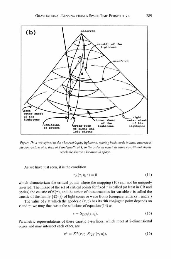
Starting at 8 = 0, r A will first increase, but because of ray focusing it may reacha maximum, then possibly decrease and become zero at 81 , corresponding to the firstpoint conjugate to the apex on the geodesic considered. Quite generally, r A vanish esexactly at conjugate points . Exactly at these points the mapping given by equation (2)for fixed T is not an immersion, i.e. there and only there 11:(T) is not a smooth hyper­surface. In the context of general relativity and optics these points are said to formthe caustic of 11:(T) , but see the remark 2 below on terminology. At the caustic, thelight "cone" has 2-dimensional edges. Moreover, in general the mapping given byequation (2) for fixed T is not injective; 11:(T) may intersect itself, see figures 1 and 2.

For fixed T , n, the function (4) is continuous for all 8 , but fails to be C 1 at conjugatepoints where it has strict minima (Seitz, Schneider, and Ehlers 1994). Between itssuccessive extrema, it can be inverted "patchwise,"

(5)

with (0:) the patch label.Another distance of an event XU on 11:(T) from xg(T) is defined by interchanging

the roles of the two events, using the future light cone of xu , a pencil proceedingfrom there to Xg(T), etc., obtaining a distance r~ which, of course, can also be cal­culated by means of Jacobi vectors, this time those which vanish at xu . According toEtherington (Etherington 1933), rA and rL are related by2

(6)

where 1 + z = hdT is the (strictly posit ive) ratio between proper time intervals at ob-r ,

server (at xg(T)) and source (at X U( T, rJ , 8)), related by light signals and measurable

as red shift z = 'xQ; 'x<.

Let us tum attention to energy-related observables. Photon conservation and raykinematics imply that the (bolometric) flux F observed at X 0 (T) with red shift z, dueto a source with luminosity L at X u(T,n,8) is given by

(7)

where rt. = (1+z)rL is called the luminosity distance of the source from the observer.Combining equat ion (7) with the definition (3) of r A and using equation (6), oneobtains the important result that the surface brightness (or integrated intensity, defined

286 JORGEN EHLERS, SIMONElTA FRIlTELLI, E ZRA T. N EWMAN

as energy/(area X time x solid angle)) 10 at the observer is related to that at the sourceIs, along a ray by

L

1 -~ - ~0 - Wo - (1 + z)4 (1 + z)4 '

(8)

provided the photons of the ray do not interact with intervening matter.The foregoing results show:(i) If the flux F and the red shift z of a source are measured and if the luminosity

L of the source can be inferred (e.g. from spectra l features or a light curve) , then r A

is determined via equations (6) and (7), i.e., indirectly measurabl e.(ii) If the true area As of an extended source can be determined and the cor­

responding solid angle WQ is measured, r A is again indirectly measurable, by equa­tion (3). As can in principle be determined by measuring curves of constant surfacebrightness in the image, i.e. on 6 (7), and relating them via equation (8) to such curveson the source's surface , where they enclose - for a particular type of source - a def­inite intrinsic area As.

In view of these (known) considerations we henceforth take r A to be measurableand , provided one could detect the patch a source is in (by the observation of multipleimages or via intergalactic absorption; ifa source has more than one image, one imagewill not belong to the first two patches), s can be replaced by rA via equation (5).

Remark 1. Though it will not be of immediate relevance to the remainder of thiswork, we nevertheless want to remark that the ideas discussed here fit into a muchlarger framework, namel y the theory of Lagrang ian and Legendrian manifolds andmaps, developed by V. I. Arnold (1980, 1986) and his colleagues. The basic idea isthat, instead of working only in the space-time itself, all the structures should be liftedto the phase-space, i.e., to the cotangent bundl e, T *9JL over the space-time. In generalmultivalued functions and singular structures (as, e.g., occur on l!:(7) at conjugatepoint s) become single-valued and smooth in the bundl e. As our basic objects arethe null geode sics that generate the past cones, they are objects to be lifted. Theedges and self intersections of the light cone mentioned in the previous discussiondisappear when lifted. Thus in addition to the parametric version of the family ofpast cones, i.e., x a = X a (7, 77 , s), we also consider the associat ed momentum four­vector field Pa = gab d:S

u

= gabLb(7, 77, s). This set of eight equations defines asmooth four dimensional submanifold, P , globally parametrized by (7,77 , s), on the(eight-dimensional) phase-space, T *9JL, of the (xa ,Pa). It is not difficult to showthat the canonical symplectic form dpa 1\ dx" ofT*9JL vanishes when restricted to P,thus P is a "Lagrangian" submanifold. The projection of P to the space-time, givenby equation (2) and referred to as a Lagrange map, is simpl y our construction of thefamily ofpast cones from the observer. The singularities of this map are the wavefrontsingularities. Though this point ofview is extremely valuable in general, we will makeno further use of it here .

We now want to first give a very general definition of a lens mapping and time ofarrival equation and then later to specialize it.

GRAVITATIONAL L ENSING FROM A SPACE-TIM E P ERSPECTIVE 287

First we temporarily consider our basic equation (2) in terms of local coordinatesX U in some region intersecting our null cones <[(T). We assume that these coordinatesX U are such that three of them , x i, are space-like and one , t , is time-like, i.e., 8~ i are

space-like vectors and tt is time-like. We then rewrite equations (2) as

(9)

Xi = X i(T, TJ , s) . (10)

In addition we assume that the Xi have been chosen such that they, or some of them,label the world lines of source points and that t measures proper time along them. (Analternate treatment would be not to spec ialize the Xi as constant on the sourcelines butto describe the sources parametrically, i.e. Xi = X~ (yI, Ts ) with constant yI .) Withthis interpretation we consider equations (9), (10) again intrinsically as giving the timeof emission, t, and the source world lines (Xi), respectively, in terms ofT, TJ , s, and wecall (9) the time of arrival functi on and (10) the generalized lens mapping. Used withequations (4) , i.e. with s (a ) = S (a ) (T, TJ , r A), the first equation describes the time ofemission of radiation from a source in terms of observable quantities, its arrival timeand direction (T, TJ ) and "distance" rA, while the second describe s the world-line ofthat source which the observer sees at time T in the direction TJ at distance rA ,

(II)

Of fundamental importance to lensing theory is the question of invertibility of thelens mapping; in other words can one uniquely write

TJ=N(Xi , T),

rA = R (Xi,T )?

(12)

(13)

Or again stated in a different way, at an observers time T , is there a unique imagedirection TJ and "distance" rA for a specific source at the position Xi? For small valuesof S or r A the answer is yes - but as S increases the gravitational field refocuses (inthe backwards direction) the rays so that eventually they cross and generically developcaustics (sharp edges in each of the past cones) which result s in multiple images ofthe same source. In figure 1, we see the world line of a source intersecting one pastcone in three places, yielding three images. In the same figure we can see the self­intersections (cross-overs) of the past rays and the formation of the caustic. The studyof multiple images is one of the main occupations of lensing experts. Here we haveassumed that the "lenses" are known - i.e. hidden in the assumed model of the space­time geometry; in practice it is the properties of the multiple image s that are used todetermine the space- time geometry.

As we have explained, a global inverse of the mapping defined by equation (10) (Tfixed) cannot be expected to exist in general. However, local invertibilityat (T, TJ , s) isequivalent to that mapp ing being a local diffeomorphism of <[(T) onto the 3-manifold(x i) of source world lines, and that holds if and only if r A(T, TJ , s) > 0, as was statedabove. If this is the case, the equations (12) and (13) provide the direction TJ anddistance r A where the observer will find the source with world line Xi at time T.

288

(a)

JURGEN E HLERS, SIMONETIA FRITIELLI, EZRA T. NEWMAN

cross-over

Figure Ia. The past lightcone 0/an observer intersec ting the worldline 0/a source at threepoints , and the three resulting image directions observed. The worldline ofthe source

intersects the inner sheet ofthe lightcone at 1, the right outer sheet at 2, the left outer sheet at3 and then continues outside ofthe cone. The lightray emitted at 1first moves on the inner

sheet, touches the caustic at c and continues on the right outer sheet to finally reach theobserver. The ray emitted at 2 moves on the right sheet to the observer. The ray emitted at 3

moves on the left sheet to the observer. The rayfrom 2 passes the cross-over line at d.

GRAVITATIONAL LENSING FROM A SPACE-TIME PERSPECTIVE 289

~rightouter sheet

of thelightconeCline

of source

(b)

.•......"..-:"I .t.left ....outer sheetof thelightcone

Figure 1b. A wavefront in the observer's past lightcone, moving backwards in time. intersectsthe sourcefirst at 3. then at 2 andfinally at 1, in the order in which its three constituent sheets

reach the source 's location in space.

As we have just seen, it is the condition

(14)

which characterizes the critical points where the mapping (10) can not be uniquelyinverted. The image of the set ofcritical points for fixed T is called (at least in GR andoptics) the caustic of Q.:(T), and the union of these caustics for variable T is called thecaustic of the family {Q.:(T)} of light cones or wave fronts (compare remarks I and 2.)

The value of s at which the geodesic (T, 'f/) has its ,8th conjugate point depends onT and n; we may thus write the solutions ofequation (14) as

(15)

Parametric representations of these caustic 3-surfaces, which meet at 2-dimensionaledges and may intersect each other, are

(16)

290 JURGEN EHLERS , SIMONElTA FRllTELLI, EZRA T. N EWM AN

observer

bigwavefront

smallwavefront

small-wavefrontsingularities

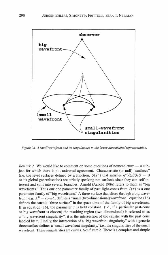
Figure 2a. A small wavefront and its singularities in the lower-dimensional representation.

Remark 2. We would like to comment on some questions of nomenclature - a sub­ject for which there is not universal agreement. Characteristic (or null) "surfaces"(i.e. the level surfaces defined by a function , S(xa) that satisfies gaboa SOb S = 0or its global generalisation) are strictly speaking not surfaces since they can self in­tersect and split into several branches; Arnold (Arnold 1986) refers to them as "bigwavefronts." Thus our one parameter family of past light-cones from \1:(T) is a oneparameter family of "big wavefronts." A three-surface that slices through a big wave­front. e.g. X O= cons i ., defines a "small (two-dimensional) wavefront." equation (16)defines the caustic "three-surface" in the space-time of the family of big wavefronts.If in equation (16), the parameter T is held constant. (i.e., if a particular past-coneor big wavefront is chosen) the resulting region (two-dimensional) is referred to asa "big wavefront singularity"; it is the intersection of the caustic with the past conelabeled by T . Finally, the intersection of a "big wavefront singularity" with a genericthree surface defines a "small wavefront singularity," i.e., the singularities of the smallwavefront. These singulariti es are curves. See figure 2. There is a complete and simple

GRAVITATIONAL LENSING FROM A SPACE-TIME PERSPECTIVE 291

Figure 2b. A small wavefront in the appropriate three-dimens ional representation,showing cusp ridges and swallowtails.

classification (Arnold 1980) of both the stable caustics and (small and big) wavefrontsingularities. We will not explore this here. We stick to the nomenclature of Arnold's ,with the exception that we call the "big wavefront singularities" also "caustics," inorder to be in agreement with usage in GR and optics.

We now want to illustrate the uses of the physical relations (7), (8) and of thelensing laws (9), (10) or their analogs in terms of r A .

Suppose a source is (conjectured to be) seen in two images with fluxes F 1 , F 2 andthe same red shift. Then, from (7),

(17)

If the source is extended and visible in two resolved images and ifcorresponding areascan be identified in the images (in terms of isophotes, e.g. using (8)) and are observed

292 JORGEN E HLERS, S IMONETIA FRlTIELLI, EZ RA T. N EWMAN

to subtend solid angles W 1, W2, then, from (3),

(18)

Thus, the ratio of the angular sizes of the images equals the flux ratio. Both the sizeof an image and its flux depend on the amount of (in general astigmatic) focusing oflight bundles by a "lens" and intervening matter. In the first case it concerns a beamcentred on the observer, in the second case, one centred on the source, the equality ofthe two kind s of magnifi cation being due to the "reciprocity law" (6). These effectsenable astronomers to observe remote galaxies which would not be visible withoutmagnification. This is the magnification effect of lensing, stripped of the (convenient ,but in principle unnecessary) comparison with fictitiou s "unlensed" sources in a ho­mogeneous background universe. If, in particular, the world line of a source intersectsthe caustic of Q:(7) , the observer will see, at time 7, a bright, short "signal" since rA

passes through zero.Assume next that a source event at x a - e.g., a supernova outburst - is seen in

two images. Then the equations

X a ( (1) ) _ X a ( (2) )(Oil) 7 1,T]1 ,rA - (0<2) 72 ,T]2,rA (19)

must hold . They impose four condit ions on the observables 7 i , tu , r~) , given gab andthe Q:(7). Again, in practice equations (19) or rather their approximate analogs, areused to determine lens parameters on which the metric depend s. In practice, the direc­tions tu, fluxes and/or angular sizes and sometimes time delays 71 -72, are observable.

4. THE SOURCE SURFACE

The discussion just given of lensing is more general than the usual treatment. To getcloser to the standard approach we introduce the idea of a "source surface"; in theusual treatment this is treated as a "source plane." The source surface is taken asa time-like hyper-surface 'I of space-time. It will represent either the surface of anextended light source evolving in time or an arbitrary two-dimensional surface that isevolving in time, which has been chosen with some special physical or mathematicalattribute - such as being at some fixed "distance" (e.g. fixed z, r A or s) from theobserver, on which arbitrary sources reside. Analytically it will be described by

(20)

where y~ = 8XT/8yA are two space-like vectors and T " = 8XT/8t is time-like. Itis convenien t to think of 'I as the produ ct 91 x 91, with 91 = {yA}, a 2-dimensionalspace of possible source posit ions and with 91 corresponding to prop er time on theworld lines with tangent T": The plan is to study the intersections of the past cones,Q:(7), from the observer £ (7), with 'I; i.e.,

(2 1)

GRAVITATIONAL LENSING FROM A SPACE-TIME PERSPECTIVE 293

For those rays from £ (r ) that intersect 'I, these four equations have solutions of theform

yA = y A (r , 17 ),

t = V (r , 17 ),

8= 5(r, 17 ).

(22)

(23)

(24)

This can be seen from the fact that each ray, (r , 17 ), which intersects 'I, does so at somespecific point (yA, t) and at some specific affine distance 8 . If a ray intersects 'I morethan once we only consider its intersection at the smallest value of 8 .

In this narrower context we define equation (22) as the "restricted" lens mapping,giving the "spatial position" on 91 of a source as seen by the observer at time r inthe 17 direction, while equation (23) is the "restricted" time of arrival equation; theemission time t, for arrival at the observer at r in the 17 direction. 8 can be relatedto r Avia equation (5). Essentially all work on lensing is related in some way toequations (22) and (23). Again an important issue is the inversion of the lens mapping;given a set yA what are the different possible observation directions at time r? Forsufficiently small 8 it is unique while for larger 8, in general, there will be multipleimages. Analytically the pathologies of the imaging arise from the vanishing of theJacobian of equation (22), i.e. from

(25)

For each r this equation defines the critical curves on the 17 sphere, {i.e. ,17 =17(r ,w), with w, a curve parameter} which when mapped, via equation (22) , to 91yield the caustic curves on 91 given by

(26)

From the work of'H , Whitney (1955), it is known that there are only two types ofstablesingularities of maps ]R2 ---+ ]R2, namely folds and cusps. The critical set consists ofnon-intersecting, smooth curves, while the caustic set consists of piecewise smoothcurves which may have cusps, and which possibly intersect each other. See figure 3.

A valuable method for analyzing the effects of the caustic on image formationis to consider on 91, a hypothetical curve - a "source curve" - (e.g. an isophotalcurve on an extended source or the trajectory of a point source) and study the inversemapping of the source curve to the celestial sphere of the observer. The morphologyof the mapping, as the source curve is deformed to cross the caustic at both the foldsand the cusps, is fairly complicated but well studied (Berry 1987). For an examplesee figure 4. If, during such a deformation, a point on the source curve leaves thethree-image region passing through the cusp, three images become very bright andmerge, at the corresponding critical curve , into a single image which remains verybright immediately after crossing. If, on the other hand , a point passes through afold , two images brighten up, merge at the critical curve and disappear, while oneimage , which remains separated from the critical curve, persists without becomingparticularly bright. A similar story holds if, instead of considering the deformation of

294 J URGEN E HLERS, S IMONElTA F RIlTELLI, EZRA T. NEWMAN

Figure 3. Typical caustics.

source curves seen by the observer at one time, one traces the images ofa single pointsource seen by the observer during some intervall of time, and if during that intervallsome sheets of the caustic of Q2(T) intersect the world line of the source.

Several important points should be emphasized. There are (theoretically) alwaysan odd number of images of a point source (except if an emission event is situatedon the caustic) - though observationally some might either not reach the observer,having been blocked by other matter, or be to weak to be seen.

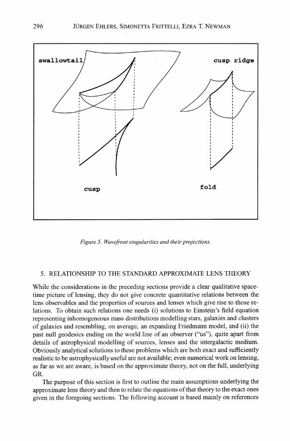
We have ju st been discussing the lens equation, equation (22), the mapping fromthe observers celestial sphere 6 (T) to 1)1. Of perhaps greater geometric significanceis the mapping from the celestial sphere to the source surface, the world-tube 'I. Geo­metrically the image is the intersection of a past cone from ,£ with 'I and is given ana­lytically by equations (22) and equation (23), the lens and time of arrival equations. Itdefines - piece-wise - a two surface in 'I, a small wave-front . The mapping fromthe two-space 6 (T) into the three space 'I is an example of what Arnold calls a Le­gendrian mapping. The stable singularities of this map, defined by the drop below twoof the rank of the map 7] f--+ (yA, t ), and referred to as wave-front singularities, arecurves (images of the critical curves of the lens map (in 6 (T)) but now in 'I insteadof in 1)1. They are classified into two types, cusp ridges and swallow-tai ls and projectto 1)1as folds and cusps. See figure 5. One can see from this perspective, why sourcesclose to caustics have bright images: there is an increase in density of source pointsthat radiate into the associated image point.

GRAV ITATIONAL LENSING FROM A SPACE-TIME P ERSPECTIVE 295

object

caust4-c,' ..................

threerays

II

II

I.I

one raycaustic;---- ....... ,

/ ,~-_J \

\II

II

/,/

---"

-1;

oimage

Figure 4. The appearance of the image of an extended object lying across caustic lines

(adaptedfram M. Berry (/987)).

Remark 3. There is a curious and surprising observation that can be made concerningthese small wavefronts. An extended source emits light, in the form of a cone of ligh­trays, continuously from each one of the points in its surface. Generally, at least oneray from each point will reach the observer, although the rays that do reach the ob­server may arrive at different times. The observation is that given any source surface'I and any observer on the curve £ , there is a (preferred) two-dimensional spacelikesection of the source surface such that the rays emitted perpendicularly to it, all arriveat the observer at the same time T . Though at first this seems difficult to visualize ­how do the rays "know" to leave perpendicularly in order to reach the observer sim­ultaneously? - , in actuality it is rather simple to see that this is so. Any displacementconfined to a null surface is either a null displacement (along a null geodesic) or isspacelike and orthogonal to the null rays. Thus any cross section (a small wavefront)of any of the past cones (as long as it is not tangent to a null direction) must be space­like and orthogonal to the rays and hence, in particular, the intersection of any pastcone with the source surface is spacelike and orthogonal to the rays. The preferredsection of the source surface is thus obtained as the intersection of the past cone andthe source surface.

296 JORGEN EHLERS, SIMONElTA FRIlTELLI, EZRA T. NEWMAN

cusp ridge

vcusp fold

Figure 5. Wavef ront singularities and their projections.

5. RELATIONSHIP TO THE STANDARD APPROXIMATE LENS THEORY

While the considerations in the preceding sections provide a clear qualitative space­time picture of lensing, they do not give concrete quanti tative relations between thelens observables and the properties of sources and lenses which give rise to those re­lations. To obtain such relations one needs (i) solutions to Einstein's field equationrepresenting inhomogeneous mass distributions modelling stars, galaxies and clustersof galaxies and resembling, on average, an expanding Friedmann model, and (ii) thepast null geodesics ending on the world line of an observer ("us") , quite apart fromdetails of astrophysical modelling of sources, lenses and the intergalactic medium.Obviously analytical solutions to these problems which are both exact and sufficientlyrealistic to be astrophysically useful are not available; even numerical work on lensing,as far as we are aware, is based on the approximate theory, not on the full, underlyingGR.

The purpose of this section is first to outline the main assumptions underlying theapproximate lens theory and then to relate the equations of that theory to the exact onesgiven in the foregoing sections . The following account is based mainly on references

GRAVITATIONAL LENSING FROM A SPACE-TIME PERSPECTIVE 297

(Schneider, Ehlers , and Falco 1992; Seitz, Schneider, and Ehlers 1994; Sasaki 1993;Holz and Wald 1998).

The first and most fundam ental assumption on which standard lens theory is (im­plicitly or explicitly) based is that a metric of the form

(27)

in which du~ is the metric of a Riemanni an 3-space Ifl of constant curvature k E{1, - 1, O}, is sufficient to describe all lens phenomena.

If it is assumed that ¢ is small compared to one, that it varies in time much moreslowly than in space and that the scale on which it varies is much smaller than theHubble scale a/a, then Einstein 's field equation for pressureless matter with densityp and a four velocity not deviating much from Ot in equation (27), can be satisfiedapproximately (in the sense of perturbation theory) by requiring that a(t) satisfiesFriedmann's equation

a 2 k3(;:) = 81T,o-3

a 2+ A,

a3,o = canst .

for the spatially averaged density ,0 and the Poisson equati on

a- 2 6.¢ = 41T(p - ,0)

(28)

(29)

(30)

hold s, with ¢ = 0.3 The symbol 6. denotes the Laplace operator assoc iated withthe metric du~ . (Additional laws have to hold for the motion of matter (Takada andFutamase 1999), but they will not be needed here.) It is important that the densityconstrast p - ,0/,0 need not be small for this approximation to be valid; in realisticappli cations that contrast is, in fact, very large compared to unity at some places.

The points (Xi) of the 3-space Ifl introduced in connection with equation (27) labelthe world lines of particles or "fundamental observers" who part icipate in the meanmotion of matter, the Hubble flow.

To proceed, one needs to make an assumption about the mass distribution in themodel universe. The simplest one - the only one to be considered here - is thatmatter consists of small "clumps" separated by vacuum . In other words , the supportof the density p is assumed to consist, at cosmic times relevant to lensing, of compactregions in Ifl, small compared to their distances and slowly moving relative to themean cosmic motion. (Other assumptions can and have been made ; for simplicity wedo not consider them here .)

Since the source of ¢ is not p, but p - ,0, whos e support at time t generically isthe whole, possibly non-compact slice t = canst . of9J1, ¢ is not "localized" at andnear the clumps. However, if one transforms the global metric of equation (27) tocoordinates T , X " which are Fermi coordinates of the underlying Friedmann metri cwith respect to a fundamental observer close to a parti cular clump , the metric takesthe form (Holz and Wald 1998)

2 1 - 2 2 1 -2 -2ds = - (1 + 2w - 3"AX )dT + (1 - 2w - fiAX )dX , (31)

298 JORGEN EHLERS, SIMONETTA FRITTELLl, EZRA T. NEWMAN

iftenns of higher than second order in the x a are neglected, where now

~w = 41fp, II' = .p + 2;p.x2 , (32)

~ denoting the ordinary Laplacian in the Xa-coordinates. Under "realistic" con­ditions equation (31) is a good approximation in any domain whose radius is muchsmaller than the Hubble radius, and even the A-tenns are negligible in such a domain.Thus, one can cover 9J1 by overlapping "nearly Newtonian" domains, "held together"by the global metric (27). The advantages of (31), (32) compared to (27), (30) is that,in each domain containing and surrounding a clump, the total density p has compactsupport , and II' can be taken to be the standard Newtonian potential which decreasesfar from the clump. (A mathematical problem may be the fitting together of the local.p's, resulting from the W's, into one smooth and globally small .p with vanishingglobal average, at least for "open" models.)

After this preparation we tum to lensing. In the approximate treatment one con­siders (apart from statistical lensing) not the whole light cone Q:(T) of the observationevent xg(T), but only a narrow angular sector of it corresponding to a small neigh­bourhood of a point TJo on the celestial sphere \5(T). One parametrizes the relevantdirections in terms of small vectors etangent to \5(T) at TJo , as indicated in figure 6,and one approximates the corresponding part of the space Q:(T) of source positions(introduced below (20» as a plane.

In order to determine the lens mapping (22), one strategy, developed independentlyin (Seitz, Schneider, and Ehlers 1994; Sasaki 1993), is to first integrate (backwards)the geodesic deviation equation

jiJa = RabcdLbLC Md

along a light ray from the observation event xg(T) to a source position yA on thesource surface 91. The result relates the infinitesimal separation dyA (of two neigh­bouring light rays, and thus) of two points on 91, to the corresponding angle deA atthe observer,

In a second step, integration of this total differential equation should then give thelens mapping, equation (22). Within the framework described above in connectionwith equations (27)-(32), each of the two steps is carried out under a simplifyingassumption.

The first assumption is that in the empty regions between observer and lens andbetween lens and source, the contribution to the geodesic deviation due to the con­formal curvature - the astigmatic Weyl focusing (Penrose 1966) - is negligiblecompared to that due to Ricci curvature (anastigmatic focusing). In other words, itis assumed that a narrow light beam picks up shear only when passing the (thin) lenswhich is represented by an effective surface mass distribution on the lens plane. Underthis (questionable) assumption, one obtains (Seitz, Schneider, and Ehlers 1994; Sasaki1993)

(33)

GRAVITATIONAL L ENSING FROM A SPACE-TIME P ERSPECTIVE 299

In this equation, D s , D L, D Ls denote the area distances of the source S and thelens L from the observer 0 and of S from L, respecti vely, computed for shearfreelight beams in the corresponding empty regions between "clumps." The deflect ionpotent ial

(34)

arises from the "localized" Weyl tensor near the lens, computed with equations (31),(32) . It depends on the mass distribution of the lens, proj ected into the lens plane;'td28' denotes the fraction of the lens mass contained in the solid angle d28 ' , seenfrom the observer. The vector

~ 2m o~a = ----:::;

D L 08is the deflection angle of a ray, see figure 7. Equation (33) contains the differentialdeflection or;/ 08, due to the tidal field of the lens. m is the Schwarzschild radius ofthe lens.

The second assumption, presum ably less critical, is that in the narrow angularsector of Q.:(T) used to model a lens phenomenon, the D's may be taken to be constant.Then, integration of equation (33) leads to

A = D 8 A _ 2m DLS o~Y S D L o8A '

where the integration constant has been absorbed into the choice of origin in the sourceplane. Using the angle iJ = Ds1y - see figure 6 - we finally rewrit e the restric ted

lens mapping 8 ~ iJ compactly as

(35)

in which

8E== J2~i: (36)is called the generalized Einstein angle.

The equations (34)-(36) are valid also for lensing in a flat background spacetime.To see this , one may begin with eqs. (31), (32) , globally on ]R4, with A = 0 and j5 = 0,and obtain eqs . (34)-(36) with obvious modifications of the preceeding arguments .Thi s "local" version of lensing applies, e.g. to microlensing of stars in the Magellaniccloud s by stars in our Milky Way galaxy or its halo .

In the cosmological case, the unob servable "empty cone distances" in eqs. (35) ,(36) can be related to the observabl e red shifts ss , ZL of source and lens and to theparameters Ho, n o, A of the Friedmann model underlying the metri c (27), if one ad­ditionaly assumes that in empty regions between clump s the relation between affineparameter s and red shift Z is (nearly) the same as in the background model. Then thegeneralized Einstein angle can be expressed as

8~ = 2mHoF (zL' se , n o, A); (37)

300 J ORGEN EHLERS, SIMO NETTA FRITTELLI , EZRA T. N EWMAN

the complicated function F has been evaluated in (Schneider, Ehlers, and Falco 1992).The time delay between two images of a source, say image I and image 2, can be

computed similarly from the difference of the path lengths and the Shapiro delays dueto the gravitational potential well of the lens. It turns out that image 2 arrives laterthan image I by the amount

{ - - ( 87/J - 87/J - ) - - - - }6 t 12 = m(l + zL) (8 1- 8 2) , ~(81 ) +~(82 - 2('l/J (8d - 'l/J (8 2 ) )88 88

(38)The formulae (34)-(38) are the main tools of approximate lens theory. Given a"background" cosmological model through (Ho,n o, Ao) and a projected mass densityt (8 ) of a lens, these equations provide the relations between the observables Z L , zs ,the image directions e corresponding to each source position fI (see figure 6), thetime delays of"signals" arriving in the images, the flux ratios of the images (via equa­tions (17) and (35), see below), and for each resolvable extended source, the intensitiesof the images in terms of the intrinsic intensity of the source (via equation (8» .

The lens mapping and the time of arrival function have been generalized to the casewhen light deflection occurs at several, well-separated "lenses." For the purpose ofweak statistical lensing one can work directly with equations (27)-(32) and the Jacobiequation for thin light bundles without using the lens equation (35), as shown in (Holzand Wald 1998). We will not deal with these extensions of the theory here.

The preceding briefreview of standard lens theory illustrates the dependence of thelensing observables on the mass distributions of the lenses which has been assumed,but not exhibited in the previous sections.

The D's of the approximate theory which occur in eqs (35), (36) refer to shearfreelight beams in empty regions between clumps, while r A in sees. 3 and 4 refers to thefull metric. Within the approximation, the "real" or "perturbed" area distance of asource point from the observer is not Ds but follows from (35) to be

(39)

This formula corresponds to equation (4); the former TJ corresponds to the present e,T is now fixed and therefore not displayed , and the dependence on the affine parameter8 is contained in the dependence of D S and D LS on 8 . Under the various assumptionsmade in this section, the "Dyer-Roeder distances" D s and D Ls can be computedas functions of Ho, n o, A and 8 .5 Because of equation (39) and the meaning of theprevious equations (3), (6) and (8), the quantity

(40)

is called the"signed magnification ." Its absolute magnitude gives the angular and fluxmagnification of an image relative to the (fictitious) "unlensed" source, and its signtells whether the image is equally (f..l > 0) or oppositely (f..l < 0) orientated as itsoriginal. Clearly, f..l has a meaning only in perturbation theory and is not observable .The ratios of the f..l-values for different images of a source are, however, observable as

GRAVITATIONAL L ENSING FROM A SPACE-TIME P ERSPECTIVE

source plane

301

I .

lens plane

L

o

Figure 6. Illustration of the lens mapping. Shown are light pa ths == null geo desics proj ectedinto 3-space. 0 : observer,L: lens, S: source. I: defl ection point. OIS: defl ected, "perturbed "

light path. OS: unperturbed light path.

relative magnifications and relative parities of these images; recall equations (17) and(18).

The caustic of the mapping (35) is given by the vanishing of the determinant inequation (39) , since under the relevant conditions, Ds > O. In the approximationconsidered that caustic is that of a "small," spatial wave front. If the observer positionand the lens are fixed, but the source plane is varied, one obtains the caustic of the lightcone C!:(T) as the union of the various small caustics. In figure 7, the null geodesicgenerators of C!:(T) are represented as broken straight lines parametrized by 8, and thewhole "two dimensional" caustic of C!:(T) can be visualized - as far as its differentialtopol ogy is concerned - as a many-sheeted, self intersecting "surface" in ]R3.

The relationship betwe en two images, considered in connection with equation (19),is now obtained by eliminating iJ from the equations (35) for 8 (l )nd 8 (2) The timedelay can then be computed from equation (38). To see the connection with equa­tion (19), one has to take into account that, during an observa tion, the source positions

302 JO RGEN EHL ERS, SIMONEITA FRlITELLI, EZ RA T. N EWMAN

~

e .:l.n

~

-f- 8-direction

lens,projected

Figure 7. The deflec tion angle vectorfi eld 5(8) in the lens plane, 5 = e in - e out .

do not change appreciably, so inequations (19) for a = i , the T ' S can be forgotten. Theresulting three equations contain the six real variables contained in 'T/ 1, 1'/2 , r~ ), r~2 ).

The approximate theory provides the solution by giving e-; as a function of 81 andthe 7'A 's by equation (39). equation (19) for a = 0 is taken care of by (38). - The re­lations discussed here become considerably more complicated in the multiple-lensin gcase; they have been treated exhaust ively and elegantly in (Petters 1996).

Can one "derive" the approximate theory from the underlying exact one? In amathematical sense, i.e., with controlled error estimates, no - that would require amuch better quantit ative understanding of generic solution classes of Einstein' s fieldequation than the one which is available now. One may, however, be able to testthe equations of the approximate theory numerically, using the exact equations indiscretized form. Unfortunately, apart from the cases of the (neutral or charged) Kerrspacetimes and that ofa static, spherically symmetric constant density star surroundedby vacuum, whose lensing properties have been determined exactly (Kerscher 1992;Kling and Newman 1999), no other tractable exact examples seem to be at hand.So, in lensing as in other cases where a complicated theory is used to make testab le

GRAVITATIONAL LENSING FROM A SPACE-TIME PERSPECTIVE 303

predictions, one is confronted with the fact: The qualitative picture can be understoodusing the exact theory; to obtain quantitative statements one has to resort to "plausible"approximations.

ACKNOWLEDGEMENT

E. T. Newman thanks the NSF for support under grant #92-05109.

NOTES

* Submitted for publication in January 2000.

I. For a systematic presentation of lens theory which contains a brief history of it and covers the majorastrophysical appl ications up to 1991, see (Schneider, Ehlers , and Falco 1992) ; for later work consult(Wambsganss 1998) and the refs. given there.

2. For a proofof (6) see , e.g. , (Schneider, Ehlers, and Falco 1992, I 14).

3. See , e .g., (Holz and Wald 1998 ; Takada and Futamase 1999) .

4 . See, e.g., (Schneider, Ehlers, and Falco 1992; Seitz , Schneider, and Ehlers 1994) .

5. See, e.g ., (Schneider, Ehlers, and Falco 1992).

REFERENCES

Arnold, V.J . 1980. Mathematical Methods ofClassical Mechanics. Berlin : Springer Verlag.- --. 1986. Catastrophy Theory . Berlin: Springer Verlag.Berry, M. V. 1987 . "Disruption of Images: the Caustic Touching Theorem." J. Opt. Soc . Amer. A4:561 .Einstein, A. 1911. "Uber den EinfluB der Schwerkraft aufdie Ausbreitung des Lichtes ." Annalen der Physik

35 :898 .---. 1915 . "Erklarung der Perihelbewegung des Merkur aus der allgemeinen Relativitiitstheorie."

Sitzungsber. PreujJ. Akad. Wiss.Etherington, J. M . H. 1933. "On the definition of distance in general relativity." Phil. Mag . 15:761.Frittelli, S., E. T. Newman, and G. Silva-Ortigoza . 1999. "The Eikonal Equation in Asymptotically Flat

Spacetimes." J. Math . Phys . 40(2) :1041-1056.Holz, D. E., and R. M. Wald. 1998. "A new method for determining cumulative gravitational lensing effects

in inhomogeneous universes." Phys. Rev. D 58:06350 I .Kerscher, Th. F. 1992 . " Lichtkegelstrukturen statischer, sphiirisch-symmetrischer Raum zeiten mit homo­

genen Zentralkorpem." Diploma thesis , Univ. Miinchen.Kling, T., and E. T. Newman. 1999 . "Null Cones in Schwarzschild Geometry." Phys . Rev. D 59: 124002.Lebach, D. E., et al. 1995 . "Measurement of the Solar Gravitational Deflection of Radio Waves using

VLBI ." Phys. Rev. Lett. 75 :1439 .Penrose, R. 1966. "General-relativistic energy flux and elementary optics ." Pg. 259 in Essays in Honor of

Vaclav Hlavaty, ed. B. Hoffmann. Bloomington: Indiana Univ. Press .Petters, A. O. 1996 . " Mathematical Aspects of Gravitational Lensing." Pg. 1117 in Proc . 7th M. GrojJmann

Meeting on GR, vol. B, eds . R. T. Jantzen and G. M . Kaiser. Singapore: World Scientific.Renn , J., T. Sauer, and J. Stachel. 1997 . "The Origin of Gravitational Lensing." Science 275: 184.Russell, H. N. 1937. Scientific American, February, 76.Sasaki, M. 1993. "Cosmological Gravitational Lens Equation: Its Validity and Limitation." Progr. Theor.

Phys . 90 :753.Schneider, P., J. Ehlers , and E. E. Falco . 1992. GravitationalLenses. New York, Berlin , Heidelberg: Springer

Verlag .

304 JORGEN EHLERS, SIMONETIA FRITIELLI, EZRA T. NEWMAN

Seitz, S., P. Schneider, and J . Ehlers . 1994 . "Light Popagation in arbitrary spacetimes and the gravitationallens approximation." Class. Quantum Grav. II:2345.

Takada , M., and T. Futama se. 1999. " Post-Newtonian Lagrangian perturbation approach to the large scalestructure formation," Phys. Rev. D.

Walsh, G., R. F. Carswell, and R. J. Weymann. 1979. Nature 279 :381.Wambsgan ss, J. 1998. "Gravitational Lensin g in Astronomy ." Living Reviews in Astrophysics, March .Whitney, H. 1955 . "Mappings of the plane into the plane." Ann. Math. 62 :374.