''1

3 jij

i

jiij

j

i uux

u

xg

x

p

Dt

uD

Reynolds-Averaged Navier-Stokes Equations -- RANS

0

i

i

x

u

4 equations; 7 unknowns

Similar situation as when we went from Cauchy’s eq to N-S eq

j

iji

i

xg

Dt

Du

1

2

2

j

i

ij

ij

x

u

x

p

x

2

21

j

i

ii

i

x

u

x

pg

Dt

Du

j

ijji x

uAuu

'' Aj = eddy viscosity [m2/s]

x

uAuu x

y

uAuv y

z

uAuw z

x

vAvu x

y

vAvv y

z

vAvw z

x

wAwu x

y

wAwv y

z

wAww z

j

ij

jiij

j

i

x

uA

xg

x

p

Dt

uD3

1

Turbulence Closure

jjj uAA

Turbulent Kinetic Energy (TKE)

An equation to describe TKE is obtained by:

multiplying the momentum equation for turbulent flow times the turbulent flow itself (scalar product)

and then do ensemble averages

Total flow = Mean plus turbulent parts = 'uU

Same for a scalar: '

Start with momentum equation (balance) for total flow: 'ii uuDt

D

and subtract momentum equation for mean flow:

Dt

uD i

yields the momentum equation for turbulent flow: Dt

Dui '

Turbulent Kinetic Energy (TKE) Equation

ijijoj

i

jiijijijoj

i eewg

x

uuueuuuup

xu

dt

d

221 2

212

21

Multiplying turbulent flow momentum equation times ui and dropping the primes (all lower case letters are turbulent or fluctuating variables)

2

21

221

221

221

wdtd

vdtd

udtd

udtd

i

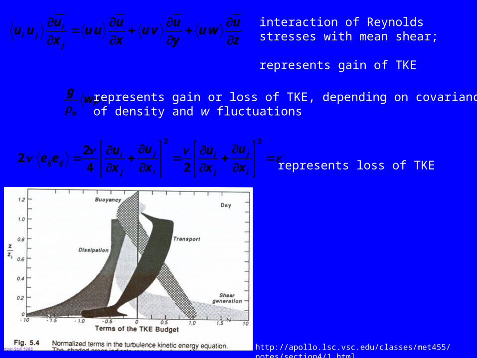
Total changes of TKE Transport of TKE Shear Production

Buoyancy Production

ViscousDissipation

i

j

j

iij x

u

xu

e21

fluctuating strain rate

Transport of TKE. Has a flux divergence form and represents spatial transport of TKE. The first two terms are transport of turbulence by turbulence itself: pressure fluctuations (waves) and turbulent transport by eddies; the third term is viscous transport

z

uwu

y

uvu

x

uuu

x

uuu

j

iji

wg

o

22

24

22

i

j

j

i

i

j

j

iijij x

u

x

u

x

u

x

uee

interaction of Reynolds stresses with mean shear;

represents gain of TKE

represents gain or loss of TKE, depending on covarianceof density and w fluctuations

represents loss of TKE

http://apollo.lsc.vsc.edu/classes/met455/notes/section4/1.html

z

uuww

g

o

0

In many ocean applications, the TKE balance is approximated as:

Injective range -- large scales where forcing injects the energy

Inertial range -- where the time required for energy transfer is shorter than the dissipative time and the energy is thus conserved and transported to smaller scales.

Dissipative range -- where the energy dissipation overcomes the transfer and the cascade is stopped.

Turbulence Production and Cascade

http://math.unice.fr/~musacchi/tesi/node9.html

KL

Inertial range

“Big whorls have little whorlsThat feed on their velocity;And little whorls have lesser whorls,And so on to viscosity.” (Lewis F Richardson, 1920)

The largest scales of turbulent motion (energy containing scales) are set by geometry:- depth of channel- distance from boundary

The rate of energy transfer to smaller scales can be estimated from scaling:

u velocity of the eddies containing energyl is the length scale of those eddies

u2 kinetic energy of eddies

l / u turnover time

u2 / (l / u ) rate of energy transfer = u3 / l ~

3

2

s

mAt any intermediate scale l, 31l~lu

But at the smallest scales LK,

413

L Kolmogorov length scale

Typically, 32616 1010 smkgW so that m~LK

310

Turbulence Cascade has a well defined structure – Kolmogorov’s K-5/3 law

Spectral power

Time (secs)

S

Frequency (Hertz)

Sp

ectr

al A

mp

(e.

g.

m2/H

z)

T = 30 s

N

n

Nknin

N

n

tnfin

eyt

eytY k

1

2

1

2

S = sin(2 π t /30)

033.0301 f

Time (secs)

S

Frequency (Hertz)

Sp

ectr

al A

mp

(e.

g.

m2/H

z)

S = sin(2 π t /30) + sin(2 π t /12)

0833.0121 f

S = sin(2 π t /30) + sin(2 π t /12) + sin(2 π t /43)

Time (secs)

S

Frequency (Hertz)

Sp

ectr

al A

mp

(e.

g.

m2/H

z)

023.0431 f

KSS ,

Wave number K (m-1)

S (

m3

s-2)

3

2

s

m

2

3

s

mS

m

K1

3532 KS

(Monismith’s Lectures)

3532 KS

P

equilibrium range

inertialdissipating range

Kolmogorov’s K-5/3 law

P & small in inertial range -- vortex stretching

Hour from 00:00 on

Data from Ichetucknee River

-5/3

3532 2

U

fS

325102 sm

(Monismith’s Lectures)

Kolmogorov’s K-5/3 law -- one of the most important results of turbulence theory