27
Rheology of Complex Fluids

Rheology of Complex Fluids


Abhijit P. Deshpande � J. Murali KrishnanP. B. Sunil KumarEditors
Rheology of Complex Fluids
ABC

EditorsAbhijit P. DeshpandeIndian Institute of Technology MadrasDepartment of Chemical EngineeringChennai [email protected]
J. Murali KrishnanIndian Institute of Technology MadrasDepartment of Civil EngineeringChennai [email protected]
P. B. Sunil KumarIndian Institute of Technology MadrasDepartment of PhysicsChennai [email protected]
ISBN 978-1-4419-6493-9 e-ISBN 978-1-4419-6494-6DOI 10.1007/978-1-4419-6494-6Springer New York Dordrecht Heidelberg London
Library of Congress Control Number: 2010936020
© Springer Science+Business Media, LLC 2010All rights reserved. This work may not be translated or copied in whole or in part without the writtenpermission of the publisher (Springer Science+Business Media, LLC, 233 Spring Street, New York,NY 10013, USA), except for brief excerpts in connection with reviews or scholarly analysis. Use inconnection with any form of information storage and retrieval, electronic adaptation, computer software,or by similar or dissimilar methodology now known or hereafter developed is forbidden.The use in this publication of trade names, trademarks, service marks, and similar terms, even if they arenot identified as such, is not to be taken as an expression of opinion as to whether or not they are subjectto proprietary rights.
Printed on acid-free paper
Springer is part of Springer Science+Business Media (www.springer.com)

Preface
In complex fluids, the atoms and molecules are organized in a hierarchy of structuresfrom nanoscopic to mesoscopic scales, which in turn make up the bulk material.Consideration of these intermediate scales of organization is essential to understandthe behaviour of the complex fluids. These fluids, an important part of what is gen-erally called soft matter, have very complex rheological responses. Many industrialsubstances encountered in chemical, personal care, food and other processing in-dustries, such as suspensions, colloidal dispersions, emulsions, powders, foams,polymeric liquids and gels, exhibit this complex behaviour. In addition, under-standing the behaviour of these complex fluids is also very important in biologicalsystems.
The area of complex fluids and soft matter has been evolving with rapid advancesin experimental and computational techniques. The main aim of this book is to in-troduce these advanced techniques, after a review of fundamental aspects. Since astudy of complex fluids involves multidisciplinary tools, contributors with differentbackgrounds have contributed chapters to this book.
The chapters in this book are based on lectures delivered in the School onRheology of Complex Fluids, held at Indian Institute of Technology Madras,Chennai during January 4–9, 2010. This school is a part of such series, earlier heldat different institutions over the last decade in India. The aim of these schools hasbeen to bring together young researchers and teachers from educational and R&Dinstitutions, and expose them to the basic concepts and research techniques usedin the study of rheological behaviour of complex fluids. These schools have beensponsored by the Department of Science and Technology, India.
The book begins with introductory chapters on non-Newtonian fluids, rheologicalresponse and fluid mechanics. This is followed by an exposition on how to under-stand multicomponent and multiphase systems, of which a lot of complex fluids areexamples. Analysis of rheological behaviour has been facilitated by experimentaland theoretical techniques. The next section of the book gives examples of these
v

vi Preface
in the form of large amplitude oscillatory shear, flow visualizations and stabilityanalysis. The remaining chapters of the book cover application areas of polymers,active fluids and granular materials and their rheology.
IIT Madras, India Abhijit P. DeshpandeApril 2010 J. Murali Krishnan
P. B. Sunil Kumar

Acknowledgements
The chapters in this book are based on lectures delivered in the School on Rhe-ology of Complex Fluids, held at Indian Institute of Technology Madras, Chennaiduring January 4–9, 2010. The school was sponsored by Science and EngineeringResearch Council, Department of Science and Technology, Government of India.We acknowledge all the participants for active discussions during the school whichhad helped in shaping the contents of this book.
Devang Khakhar, R P Chhabra, K S Gandhi and Sriram Ramaswamy played animportant role in deciding the topics presented here. We thank them for their advice.
We thank R P Chhabra, V Kumaran, K R Rajagopal, S Pushpavanam, RamaGovindarajan, Arti Dua, P Sunthar, Gautam Menon and Mehrdad Massoudi for theircontributions. Their help in providing lecture notes, draft chapters and proofreadingis acknowledged.
We thank the patient typesetting support provided by VALARDOCS and theirteam through several modifications of the chapters. Editorial assistance from San-tosh was very crucial in bringing the book to its present form. Brett Kurzman andAmanda Davis from Springer helped us in getting through different stages of thebook preparation.
Murali Krishnan would like to thank Mary Yvonne Lanzerotti for her encourage-ment in the earlier stages of this book preparation.
We also acknowledge the support provided by Indian Institute of TechnologyMadras during different stages of this book preparation.
IIT Madras, India Abhijit P. DeshpandeApril 2010 J. Murali Krishnan
P. B. Sunil Kumar
vii


Contents
Part I Background
1 Non-Newtonian Fluids: An Introduction . . . . . . . . . . . . . . . . . . . . . . . . . . . . . . . . . . 3Rajendra P. Chhabra
2 Fundamentals of Rheology . . . . . . . . . . . . . . . . . . . . . . . . . . . . . . . . . . . . . . . . . . . . . . . . . . 35V. Kumaran
3 Mechanics of Liquid Mixtures . . . . . . . . . . . . . . . . . . . . . . . . . . . . . . . . . . . . . . . . . . . . . . 67Kumbakonam Ramamani Rajagopal
Part II Rheology
4 Oscillatory Shear Rheology for Probing NonlinearViscoelasticity of Complex Fluids: Large AmplitudeOscillatory Shear . . . . . . . . . . . . . . . . . . . . . . . . . . . . . . . . . . . . . . . . . . . . . . . . . . . . . . . . . . . . . 87Abhijit P. Deshpande
5 PIV Techniques in Experimental Measurement of TwoPhase (Gas–Liquid) Systems . . . . . . . . . . . . . . . . . . . . . . . . . . . . . . . . . . . . . . . . . . . . . . . .111Basheer Ashraf Ali and Subramaniam Pushpavanam
6 An Introduction to Hydrodynamic Stability . . . . . . . . . . . . . . . . . . . . . . . . . . . . . . .131Anubhab Roy and Rama Govindarajan
Part III Applications
7 Statics and Dynamics of Dilute Polymer Solutions . . . . . . . . . . . . . . . . . . . . . . .151Arti Dua
8 Polymer Rheology . . . . . . . . . . . . . . . . . . . . . . . . . . . . . . . . . . . . . . . . . . . . . . . . . . . . . . . . . . . .171P. Sunthar
ix

x Contents
9 Active Matter . . . . . . . . . . . . . . . . . . . . . . . . . . . . . . . . . . . . . . . . . . . . . . . . . . . . . . . . . . . . . . . . .193Gautam I. Menon
10 Mathematical Modelling of Granular Materials . . . . . . . . . . . . . . . . . . . . . . . . . .219Mehrdad Massoudi
Author Index . . . . . . . . . . . . . . . . . . . . . . . . . . . . . . . . . . . . . . . . . . . . . . . . . . . . . . . . . . . . . . . . . . . . . . . .247
Subject Index . . . . . . . . . . . . . . . . . . . . . . . . . . . . . . . . . . . . . . . . . . . . . . . . . . . . . . . . . . . . . . . . . . . . . . .253

Contributors
Basheer Ashraf Ali Research Scholar, Indian Institute of Technology Madras,Chennai 600036, India, [email protected]
Rajendra P. Chhabra Department of Chemical Engineering, Indian Instituteof Technology Kanpur 208016, India, [email protected]
Abhijit P. Deshpande Indian Institute of Technology Madras, Chennai 600036,India, [email protected]
Arti Dua Department of Chemistry, Indian Institute of Technology Madras,Chennai 600036, India, [email protected]
Rama Govindarajan Engineering Mechanics Unit, Jawaharlal Nehru Centrefor Advanced Scientific Research, Jakkur, Bangalore 560064, India,[email protected]
V. Kumaran Department of Chemical Engineering, Indian Institute of Science,Bangalore 560 012, India, [email protected]
Mehrdad Massoudi U.S. Department of Energy, National Energy TechnologyLaboratory (NETL), Pittsburgh, PA 15236, USA, [email protected]
Gautam I. Menon The Institute of Mathematical Sciences, CIT Campus,Taramani, Chennai 600113, India, [email protected]
Subramaniam Pushpavanam Professor, Indian Institute of Technology Madras,Chennai 600036, India, [email protected]
Kumbakonam Ramamani Rajagopal Department of Mechanical Engineering,Texas A&M University, College Station, TX 77845, USA, [email protected]
Anubhab Roy Engineering Mechanics Unit, Jawaharlal Nehru Centrefor Advanced Scientific Research, Jakkur, Bangalore 560064, India,[email protected]
P. Sunthar Department of Chemical Engineering, Indian Institute of TechnologyBombay, Mumbai 400076, India, [email protected]
xi


Acronyms
BSW Baumgartel, Schausberger and Winter spectrumCCD Charge Coupled DeviceCFD Computational Fluid DynamicsFENE Finitely Extensible Nonlinear ElasticityGNF Generalized Newtonian FluidsLASER Light Amplification by Stimulated Emission of Light RadiationLAOS Large Amplitude Oscillatory ShearLDV Laser Doppler VelocimetryPIB PolyisobutylenePIV Particle Image VelocimetryPM Parsimonious Model SpectrumPMFI Principle of Material Frame-IndifferencePMMA PolymethylmethacrylateSAOS Small Amplitude Oscillatory ShearSSP Self-Sustaining ProcessVIBGYOR Violet, Indigo, Blue, Green, Yellow, Orange, RedWLC Wormlike Chain
xiii


Part IBackground

Chapter 1Non-Newtonian Fluids: An Introduction
Rajendra P. Chhabra
Abstract The objective of this chapter is to introduce and to illustrate the frequentand wide occurrence of non-Newtonian fluid behaviour in a diverse range ofapplications, both in nature and in technology. Starting with the definition of anon-Newtonian fluid, different types of non-Newtonian characteristics are brieflydescribed. Representative examples of materials (foams, suspensions, polymersolutions and melts), which, under appropriate circumstances, display shear-thinning, shear-thickening, visco-plastic, time-dependent and viscoelastic behaviourare presented. Each type of non-Newtonian fluid behaviour has been illustrated viaexperimental data on real materials. This is followed by a short discussion onhow to engineer non-Newtonian flow characteristics of a product for its satisfac-tory end use by manipulating its microstructure by controlling physico-chemicalaspects of the system. Finally, we touch upon the ultimate question about the roleof non-Newtonian characteristics on the analysis and modelling of the processes ofpragmatic engineering significance.
1.1 Introduction
Most low-molecular-weight substances such as organic and inorganic liquids,solutions of low-molecular-weight inorganic salts, molten metals and salts andgases exhibit Newtonian flow characteristics, i.e., at constant temperature and pres-sure, in simple shear, the shear stress .� / is proportional to the rate of shear . P�/ andthe constant of proportionality is the familiar dynamic viscosity .�/. Such fluids areclassically known as the Newtonian fluids, albeit the notion of flow and of viscositypredates Newton [40]. For most liquids, the viscosity decreases with temperature
R.P. Chhabra (�)Department of Chemical Engineering, Indian Institute of Technology, Kanpur 208016, Indiae-mail: [email protected]
J.M. Krishnan et al. (eds.), Rheology of Complex Fluids,DOI 10.1007/978-1-4419-6494-6 1, © Springer Science+Business Media, LLC 2010
3

4 R.P. Chhabra
Table 1.1 Values ofviscosity for common fluidsat room temperature
Substance �(Pa s)
Air 10�5
Water 10�3
Ethyl alcohol 1:2 � 10�3
Mercury 1:5 � 10�3
Ethylene glycol 20 � 10�3
Olive oil 0.1100% Glycerol 1.5Honey 10Corn syrup 100Bitumen 108
Molten glass 1012
and increases with pressure. For gases, it increases with both temperature andpressure [35]. Broadly, higher the viscosity of a substance, more the resistance itpresents to flow (and hence more difficult to pump!). Table 1.1 provides typicalvalues of viscosity for scores of common fluids [12]. As we go down in the table,the viscosity increases by several orders of magnitude, and thus one can argue that asolid can be treated as a fluid whose viscosity tends towards infinity, � ! 1. Thus,the distinction between a fluid and a solid is not as sharp as we would like to think!Ever since the formulation of the equations of continuity (mass) and momentum(Cauchy, Navier–Stokes), the fluid dynamics of Newtonian fluids has come a longway during the past 300 or so years, albeit significant challenges especially in thefield of turbulence and multiphase flows still remain. During the past 50–60 years,there has been a growing recognition of the fact that many substances of industrialsignificance, especially of multiphase nature (foams, emulsions, dispersions andsuspensions, slurries, for instance) and polymeric melts and solutions (both naturaland manmade) do not conform to the Newtonian postulate of the linear relation-ship between � and P� in simple shear, for instance. Accordingly, these fluids arevariously known as non-Newtonian, non-linear, complex or rheologically complexfluids. Table 1.2 gives a representative list of fluids, which exhibit different kindsand varying severity of non-Newtonian flow behaviour [12]. Indeed, so widespreadis the non-Newtonian fluid behaviour in nature and in technology that it would beno exaggeration to say that the Newtonian fluid behaviour is an exception ratherthan the rule! This chapter endeavours to provide a brief introduction to the differentkinds of non-Newtonian flow characteristics, their characterization and implicationsin engineering applications. The material presented herein is mainly drawn from ourrecent books [11, 12]. The assumptions of material isotropy and incompressibilityare implicit throughout our discussion.

1 Non-Newtonian Fluids: An Introduction 5
Table 1.2 Examples of substances exhibiting non-Newtonian fluid behaviour
Adhesives (wall paper paste, carpet adhesive,for instance)
Food stuffs (Fruit/vegetable purees andconcentrates, sauces, salad dressings,mayonnaise, jams and marmalades,ice-cream, soups, cake mixes and caketoppings, egg white, bread mixes, snacks)
Ales (beer, liqueurs, etc.) Greases and lubricating oilsAnimal waste slurries from cattle farms Mine tailings and mineral suspensionsBiological fluids (blood, synovial fluid,
saliva, etc.)Molten lava and magmas
Bitumen Paints, polishes and varnishesCement paste and slurries Paper pulp suspensionsChalk slurries Peat and lignite slurriesChocolates Polymer melts and solutions, reinforced
plastics, rubberCoal slurries Printing colors and inksCosmetics and personal care products (nail
polish, lotions and creams, lipsticks,shampoos, shaving foams and creams,toothpaste, etc.)
Pharmaceutical products (creams, foams,suspensions, for instance)
Dairy products and dairy waste streams(cheese, butter, yogurt, fresh cream, whey,for instance)
Sewage sludge
Drilling muds Wet beach sandFire fighting foams Waxy crude oils
1.2 Classification of Fluid Behaviour
1.2.1 Definition of a Newtonian Fluid
It is useful to begin with the definition of a Newtonian fluid. In simple shear(Fig. 1.1), the response of a Newtonian fluid is characterized by a linear relation-ship between the applied shear stress and the rate of shear, i.e.,
�yx D F
AD � P�yx: (1.1)
Figure 1.2 shows experimental results for corn syrup and for cooking oil confirm-ing their Newtonian fluid behaviour; the flow curves pass through the origin and theviscosity values are � D 11:6Pa s for corn syrup and � D 64mPa s for the cookingoil. Figure 1.1 and (1.1), of course, represent the simplest case wherein there is onlyone non-zero component of velocity, Vx , which is a function of y. For the generalcase of three-dimensional flow (Fig. 1.3), clearly there are six shearing and threenormal components of the stress tensor, S. It is customary to split the total stressinto an isotropic part (pressure, p) and a deviatoric part as
S D �pI C � ; (1.2)

6 R.P. Chhabra
Fig. 1.1 Schematicrepresentation of aunidirectional shearing flow
dVxFSurface area, A
x
y
σyx
Fig. 1.2 Typical shearstress–shear rate data fortwo Newtonian fluids
where � is traceless, i.e., tr � � D 0, and pressure is consistent with the continu-ity equation. The trace-free requirement together with the physical requirement ofsymmetry � D � T implies that there are only three independent shear components(off-diagonal elements) and two normal stress differences (diagonal elements) of thedeviatoric stress. Thus, in Cartesian coordinates, these are �xy.D �yx/, �xz.D �zx/
and �yz.D �zy/, and the two normal stress differences are defined as
Primary normal stress difference,N1 D �xx � �yy; (1.3)
Secondary normal stress difference,N2 D �yy � �zz: (1.4)
For Newtonian fluids, these components are related linearly to the rate of defor-mation of tensor components via the scalar viscosity. For instance, the three stress
1 Non-Newtonian Fluids: An Introduction 7
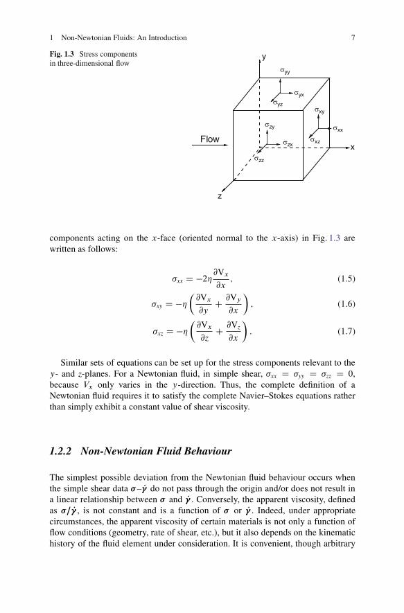
Fig. 1.3 Stress componentsin three-dimensional flow
y
z
x
σyy
σyz
σzy
σzxσxz
σxx
σxy
σzz
σyx
Flow
components acting on the x-face (oriented normal to the x-axis) in Fig. 1.3 arewritten as follows:
�xx D �2�@Vx@x
; (1.5)
�xy D ���@Vx@y
C @Vy@x
�; (1.6)
�xz D ���@Vx@z
C @Vz
@x
�: (1.7)
Similar sets of equations can be set up for the stress components relevant to they- and z-planes. For a Newtonian fluid, in simple shear, �xx D �yy D �zz D 0,because Vx only varies in the y-direction. Thus, the complete definition of aNewtonian fluid requires it to satisfy the complete Navier–Stokes equations ratherthan simply exhibit a constant value of shear viscosity.
1.2.2 Non-Newtonian Fluid Behaviour
The simplest possible deviation from the Newtonian fluid behaviour occurs whenthe simple shear data �– P� do not pass through the origin and/or does not result ina linear relationship between � and P� . Conversely, the apparent viscosity, definedas �= P� , is not constant and is a function of � or P� . Indeed, under appropriatecircumstances, the apparent viscosity of certain materials is not only a function offlow conditions (geometry, rate of shear, etc.), but it also depends on the kinematichistory of the fluid element under consideration. It is convenient, though arbitrary

8 R.P. Chhabra
(and probably unscientific too), to group such materials into the following threecategories:
1. Systems for which the value of P� at a point within the fluid is determined only bythe current value of � at that point, or vice versa, these substances are variouslyknown as purely viscous, inelastic, time-independent or generalized Newtonianfluids (GNF);
2. Systems for which the relation between � and P� shows further dependence onthe duration of shearing and kinematic history; these are called time-dependentfluids, and finally,
3. Systems which exhibit a blend of viscous fluid-like behaviour and of elastic solid-like behaviour. For instance, this class of materials shows partial elastic recovery,recoil, creep, etc. Accordingly, these are called viscoelastic or elastico-viscousfluids.
As noted earlier, the aforementioned classification scheme is quite arbitrary,though convenient, because most real materials often display a combination of twoor even all these types of features under appropriate circumstances. For instance,it is not uncommon for a polymer melt to show time-independent (shear-thinning)and viscoelastic behaviour simultaneously and for a china clay suspension to exhibita combination of time-independent (shear-thinning or shear-thickening) and time-dependent (thixotropic) features at certain concentrations and/or at appropriate shearrates. Generally, it is, however, possible to identify the dominant non-Newtonianaspect and to use it as a basis for the subsequent process calculations. Each type ofnon-Newtonian fluid behaviour is now dealt with in more detail.
1.3 Time-Independent Fluid Behaviour
As noted above, in simple unidirectional shear, this subset of fluids is characterizedby the fact that the current value of the rate of shear at a point in the fluid is deter-mined only by the corresponding current value of the shear stress and vice versa.Conversely, one can say that such fluids have no memory of their past history. Thus,their steady shear behaviour may be described by a relation of the form,
P�yx D f .�yx/; (1.8)
or, its inverse form,�yx D f �1. P�yx/: (1.9)
Depending upon the form of (1.8) or (1.9), three possibilities exist:
1. Shear-thinning or pseudoplastic behavior2. Visco-plastic behaviour with or without shear-thinning behaviour3. Shear-thickening or dilatant behaviour.

1 Non-Newtonian Fluids: An Introduction 9
Fig. 1.4 Qualitative flowcurves for different typesof non-Newtonian fluids
Figure 1.4 shows qualitatively the flow curves (also called rheograms) on linearcoordinates for the above-noted three categories of fluid behaviour; the linear rela-tion typical of Newtonian fluids is also included in Fig. 1.4.
1.3.1 Shear-Thinning Fluids
This is perhaps the most widely encountered type of time-independent non-Newtonian fluid behaviour in engineering practice. It is characterized by an apparentviscosity � (defined as �yx= P�yx), which gradually decreases with increasing shearrate. In polymeric systems (melts and solutions), at low shear rates, the apparentviscosity approaches a Newtonian plateau, where the viscosity is independent ofshear rate (zero shear viscosity, �
0).
limP�yx!0
�yx
P�yxD �
0: (1.10)
Furthermore, polymer solutions also exhibit a similar plateau at very high shear rates(infinite shear viscosity, �
1
), i.e.,
limP�yx!1
�yx
P�yxD �
1
: (1.11)
In most cases, the value of �1
is only slightly higher than the solvent viscosity �s .Figure 1.5 shows this behaviour in a polymer solution embracing the full spectrum

10 R.P. Chhabra
Fig. 1.5 Demonstration of zero-shear and infinite shear viscosities for a polymer solution
of values going from �0
to �1
. Obviously, the infinite-shear limit is not seen forpolymer melts and blends, or foams or emulsions or suspensions. Thus, the appar-ent viscosity of a pseudoplastic substance decreases with the increasing shear rate,as shown in Fig. 1.6 for three polymer solutions where not only the values of �
0are
seen to be different in each case, but the rate of decrease of viscosity with shear rateis also seen to vary from one system to another as well as with the shear rate inter-val considered. Finally, the value of shear rate marking the onset of shear-thinningis influenced by several factors such as the nature and concentration of polymer, thenature of solvent, etc. for polymer solutions and particle size, shape, concentrationof solids in suspensions, for instance. Therefore, it is impossible to suggest validgeneralizations, but many polymeric systems exhibit the zero-shear viscosity regionbelow P� < 10�2 s�1. Usually, the zero-shear viscosity region expands as the molec-ular weight of polymer falls, or its molecular weight distribution becomes narrower,as the concentration of polymer in the solution is reduced.
The next question which immediately comes to mind is that how do we approxi-mate this type of fluid behaviour? Over the past 100 years or so, many mathematicalequations of varying complexity and forms have been reported in the literature;some of these are straightforward attempts at curve fitting the experimental data(�– P�), while others have some theoretical basis (blended with empiricism) in sta-tistical mechanics as an extension of the application of kinetic theory to the liquidstate, etc. [9]. While extensive listing of viscosity models is available in severalbooks, for e.g., see Ibarz and Barbosa–Canovas [23] and Govier and Aziz [19], arepresentative selection of widely used expressions is given here.

1 Non-Newtonian Fluids: An Introduction 11
Fig. 1.6 Representative shear stress and apparent viscosity behaviour for three pseudoplastic poly-mer solutions
1.3.1.1 Power Law or Ostwald de Waele Equation
Often the relationship between shear stress (� ) and shear rate ( P�) plotted on log–logcoordinates for a shear-thinning fluid can be approximated by a straight line over aninterval of shear rate, i.e.,
� D m. P�/n; (1.12)
or, in terms of the apparent viscosity,
� D m. P�/n�1: (1.13)
Obviously, 0 < n < 1 will yield .d�=d P�/ < 0, i.e., shear-thinning behaviour offluids is characterized by value of n (power-law index) smaller than unity. Manypolymer melts and solutions exhibit the value of n in the range 0.3–0.7 depend-ing upon the concentration and molecular weight of the polymer, etc. Even smallervalues of power-law index (n �0.1 – 0.15) are encountered with fine particle sus-pensions like kaolin-in-water, bentonite-in-water, etc. Naturally, smaller the valueof n, more shear-thinning is the material. The other constant,m (consistency index),is a measure of the consistency of the substance.
Although (1.12) or (1.13) offers the simplest approximation of shear-thinningbehaviour, it predicts neither the upper nor the lower Newtonian plateau in the limitsof P� ! 0 or P� ! 1. Besides, the values of m and n are reasonably constant onlyover a narrow interval of shear rate range whence one needs to know a priori thelikely range of shear rate to be encountered in an envisaged application.

12 R.P. Chhabra
1.3.1.2 The Cross Viscosity Equation
In order to rectify some of the weaknesses of the power-law, Cross [14] presentedthe following empirical form, which has gained wide acceptance in the literature. Insimple shear, it is written as
� � �1
�0
� �1
D 1
1Cm. P�/n : (1.14)
It is readily seen that for n < 1, this model also predicts shear-thinning behaviour.Furthermore, the Newtonian limit is recovered here when m ! 0. Though initiallyCross [14] proposed that n D 2=3 was satisfactory for numerous substances, it isnow thought that treating it as an adjustable parameter offers significant improve-ment in terms of the degree of fit [5]. Evidently, (1.14) correctly predicts � D �
0
and � D �1
in the limits of P� ! 0 and P� ! 1, respectively.
1.3.1.3 The Ellis Fluid Model
While the two viscosity models presented thus far are examples of the form of (1.9),the Ellis model is an illustration of the inverse form, (1.8). In unidirectional simpleshear, it is written as
� D �0
1C�
��
1=2
�˛�1 : (1.15)
In (1.15), �0
is the zero-shear viscosity and the remaining two parameters �1=2
and ˛ > 1 are adjusted to obtain the best fit to a given set of data. Clearly, ˛ > 1
yields the decreasing values of shear viscosity with increasing shear rate. It is readilyseen that the Newtonian limit is recovered by setting �
1=2! 1. Furthermore, when
.�=�1=2/ � 1, (1.15) reduces to the power-law model, (1.12) or (1.13).
1.3.2 Visco-Plastic Fluid Behaviour
This type of non-Newtonian fluid behaviour is characterized by the existence ofa threshold stress (called yield stress or apparent yield stress, �0), which must beexceeded for the fluid to deform (shear) or flow. Conversely, such a substance willbehave like an elastic solid (or flow en masse like a rigid body) when the externallyapplied stress is less than the yield stress, �
0. Of course, once the magnitude of the
external yield stress exceeds the value of �0, the fluid may exhibit Newtonian be-
haviour (constant value of �) or shear-thinning characteristics, i.e., �. P�/. It thereforestands to reason that, in the absence of surface tension effects, such a material willnot level out under gravity to form an absolutely flat free surface. Quantitatively, thistype of behaviour can be hypothesized as follows: such a substance at rest consistsof three-dimensional structures of sufficient rigidity to resist any external stress less

1 Non-Newtonian Fluids: An Introduction 13
thanˇ�
0
ˇand therefore offers an enormous resistance to flow, albeit it still might
deform elastically. For stress levels aboveˇ�
0
ˇ, however, the structure breaks down
and the substance behaves like a viscous material. In some cases, the build-up andbreakdown of structure has been found to be reversible, i.e., the substance may re-gain its (initial or somewhat lower) value of the yield stress following a long periodof rest.
A fluid with a linear flow curve for j� j > ˇ�
0
ˇis called a Bingham plastic fluid,
and is characterized by a constant value of viscosity �B . Thus, in one-dimensionalshear, the Bingham model is written as:
�yx D �B
0C �B P�yx
ˇ�yx
ˇ>ˇ�
B
0
ˇ(1.16a)
P�yx D 0ˇ�yx
ˇ<ˇˇ�B
0
ˇˇ (1.16b)
On the other hand, a visco-plastic material showing shear-thinning behaviour atstress levels exceeding
ˇ�
0
ˇis known as a yield-pseudoplastic fluid, and its be-
haviour is frequently approximated by the so-called Herschel–Bulkley fluid modelwritten for 1-D shear flow as follows:
�yx D �H
0Cm. P�yx/
nˇ�yx
ˇ>ˇ�
H
0
ˇ(1.17a)
P�yx D 0ˇ�yx
ˇ<ˇˇ�H
0
ˇˇ (1.17b)
Another commonly used viscosity model for visco-plastic fluids is the so-calledCasson model, which has its origins in modelling the flow of blood, but it has beenfound a good approximation for many other substances also [5, 6]. It is written as:
qˇ�yx
ˇ Dqˇ�
C
0
ˇCq�C
ˇ P�yx
ˇ ˇ�yx
ˇ>ˇ�
C
0
ˇ(1.18a)
P�yx D 0ˇ�yx
ˇ<ˇˇ�C
0
ˇˇ (1.18b)
While qualitative flow curves for a Bingham fluid and for a yield-pseudoplasticfluid are included in Fig. 1.4, experimental data for a synthetic polymer solutionand a meat extract are shown in Fig. 1.7. The meat extract (�
0D 17Pa) conforms
to (1.16), whereas the carbopol solution (�0
D 68Pa) shows yield-pseudoplasticbehaviour.
Typical examples of yield-stress fluids include blood, yoghurt, tomato puree,molten chocolate, tomato sauce, cosmetics, nail polishes, foams, suspensions, etc.Thorough reviews on the rheology and fluid mechanics of visco-plastic fluids areavailable in the literature [3, 6].
Finally, before leaving this subsection, it is appropriate to mention here that ithas long been a matter of debate and discussion in the literature whether a true yieldstress exists or not, e.g., see the trail-blazing paper of Barnes and Walters [4] and thereview of Barnes [3] for different viewpoints on this matter. Many workers view the

14 R.P. Chhabra
Fig. 1.7 Shear stress–shear rate data for a meat extract and for a carbopol solution displayingBingham plastic and visco-plastic behaviours, respectively
yield stress in terms of a transition from solid-like behaviour to fluid-like behaviourwhich manifests itself in terms of an abrupt decrease in viscosity (by several ordersof magnitude in many substances) over an extremely narrow range of shear rate [43].Evidently, the answer to the question whether a substance has a yield stress or notseems to be closely related to the choice of a time scale of observation. In spite ofthis fundamental difficulty, the notion of an apparent yield stress is of considerablevalue in the context of engineering applications, especially for product developmentand design in food, pharmaceutical and health care sectors [3, 36].
1.3.3 Shear-Thickening or Dilatant Behaviour
This class of fluids is similar to pseudoplastic systems in that it shows no yield stress,but its apparent viscosity increases with the increasing shear rate and hence the nameshear-thickening. Originally, this type of behaviour was observed in concentratedsuspensions, and one can qualitatively explain it as follows: at rest, the voidage ofthe suspension is minimum and the liquid present in the sample is sufficient to fillthe voids completely. At low shearing levels, the liquid lubricates the motion ofeach particle past another thereby minimizing solid–solid friction. Consequently,the resulting stresses are small. At high shear rates, however, the mixture expands(dilates) slightly (similar to that seen in sand dunes) so that the available liquid isno longer sufficient to fill the increased void space and to prevent direct solid–solidcontacts (and friction). This leads to the development of much larger shear stresses


