Rheology of Giant Micelles - arXiv · RHEOLOGY OF GIANT MICELLES 1.1 Introduction An amphiphilic...

arX

iv:c

ond-

mat

/070

2047

v1 [

cond

-mat

.sof

t] 2

Feb

200

7

Chapter 1

Rheology of Giant Micelles

M. E. Cates, SUPA School of Physics, University of Edinburgh, JCMB Kings Buildings,Mayfield Road, Edinburgh EH9 3JZ, United KingdomandS. M. Fielding, School of Mathematics, University of Manchester, Booth Street East,Manchester M13 9EP, United Kingdom

Abstract: Giant micelles are elongated, polymer-like objects created by the self-assemblyof amphiphilic molecules (such as detergents) in solution. Giant micelles are typically flexible,and can become highly entangled even at modest concentrations. The resulting viscoelasticsolutions show fascinating flow behaviour (rheology) which we address theoretically in thisarticle at two levels. First, we summarise advances in understanding linear viscoelasticspectra and steady-state nonlinear flows, based on microscopic constitutive models thatcombine the physics of polymer entanglement with the reversible kinetics of self-assembly.Such models were first introduced two decades ago, and since then have been shown toexplain robustly several distinctive features of the rheology in the strongly entangled regime,including extreme shear-thinning. We then turn to more complex rheological phenomena,particularly involving spatial heterogeneity, spontaneous oscillation, instability, and chaos.Recent understanding of these complex flows is based largely on grossly simplified modelswhich capture in outline just a few pertinent microscopic features, such as coupling betweenstresses and other order parameters such as concentration. The role of ‘structural memory’(the dependence of structural parameters such as the micellar length distribution on the flowhistory) in explaining these highly nonlinear phenomena is addressed. Structural memoryalso plays an intriguing role in the little-understood shear-thickening regime, which occursin a concentration regime close to but below the onset of strong entanglement, and which ismarked by a shear-induced transformation from an inviscid to a gelatinous state.1

1This is a preprint of an article whose final and definitive form has been published in Advances in Physics (c) 2006 copyrightTaylor & Francis; Advances in Physics is available online at http://journalsonline.tandf.co.uk/. The URL of the article ishttp://journalsonline.tandf.co.uk/openurl.asp?genre=article&id=doi:10.1080/00018730601082029.

1

http://arXiv.org/abs/cond-mat/0702047v1

http://journalsonline.tandf.co.uk/

http://journalsonline.tandf.co.uk/openurl.asp?genre=article

2 CHAPTER 1. RHEOLOGY OF GIANT MICELLES

1.1 Introduction

An amphiphilic molecule is one that combines a water-loving (hydrophilic) part or ‘headgroup’ with a with a water-hating (hydrophobic) part or ‘tail’. The head-group can beionic, so that the molecule becomes charged by dissociation in aqueous solution; or nonionic(but highly polar, favouring a water environment), in which case the amphiphile remainsuncharged. Zwitterionic head-groups, with two charges of opposite sign, are also common.The hydrophobic tail is almost always a short hydrocarbon (though fluorocarbons can alsobe used); in some cases (such as biological lipids) there are two tails. The most importantproperty of amphiphilic molecules, from the viewpoint of theoretical physics at least, is theirtendency to self-assemble by aggregating reversibly into larger objects. The simplest of theseis a spherical aggregate called a ‘micelle’ which in water has the hydrophobic tails sequesteredat the centre, coated by a layer of headgroups; see Fig.1.1. (In a nonaqueous solvent, thestructure can be inverted to create a ‘reverse micelle’.)

For geometrical reasons, a spherical micelle is self-limiting in size: unless the amphiphilicsolution contains a third molecular component (an oil) that can fill any hole in the middle,the radius of a micelle cannot be more than about twice the length of the amphiphile. Toavoid exposing tails to water, it also cannot be much less than this; the resulting ‘quorum’ ofa few tens of molecules for creation of a stable micelle leads to a sharp minimum in free energyas a function of aggregation number. This collective aspect to micelle formation causes thetransition from a molecularly dispersed solution to one of micelles to be rather sharp; micellesproliferate abruptly when the concentration is raised above the ‘critical micelle concentration’or CMC [1].

In a spherical micelle the volume ratio of head- and tail-rich regions is also essentiallyfixed: such micelles are favoured by amphiphiles with relatively large size ratios between headand tail. Suppose this size ratio is smoothly decreased, for instance by adding salt to anionic micellar solution (effectively reducing the head-group size by screening the coulombicrepulsions). The most stable local packing then evolves from the spherical micelle towards acylinder; Fig.1.1. (Proceeding further, it becomes a flat bilayer; systems in which this hap-pens are not addressed here.) Allowing for entropy, the transition from spheres to cylindersis not sudden, but proceeds via short cylindrical micelles with hemispherical end-caps. Thebodies of these cylinders smoothly increase in length as the packing energy of the body fallsrelative to the caps; the micelles eventually become extremely long. The law of mass action,which favours larger aggregates, means that in suitable systems the same sequence can beobserved by increasing concentration at fixed head/tail size ratio (fixed ionic strength).

Since the organization of amphiphiles within the cylindrical body is (in most cases) fluid-like, the resulting ‘giant micelles’ soon exceed the so-called persistence length, at which ther-mal motion overcomes the local rigity and the micelle resembles a flexible polymer chain.This crossover may or may not precede the ‘overlap threshold’ at which the volume occu-pied by a micelle – the smallest sphere that contains it – overlaps with other such volumes.Beyond this threshold, the chainlike objects soon become entangled but (unless extremelystiff) remain in an isotropic phase with no long-range orientational order. At very high con-centrations, such ordering can arise, as can positional order, giving for example a hexagonalarray of near-infinite straight cylinders. Branching of micelles can also be important in bothisotropic and ordered phases; a schematic phase diagram, applicable to many but not allsystems containing giant micelles, is shown in Fig.1.1.

This article addresses primarily the isotropic phase of giant micelles, in a concentration

1.1. INTRODUCTION 3

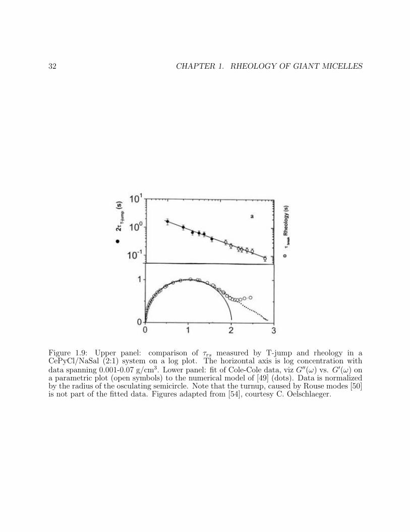
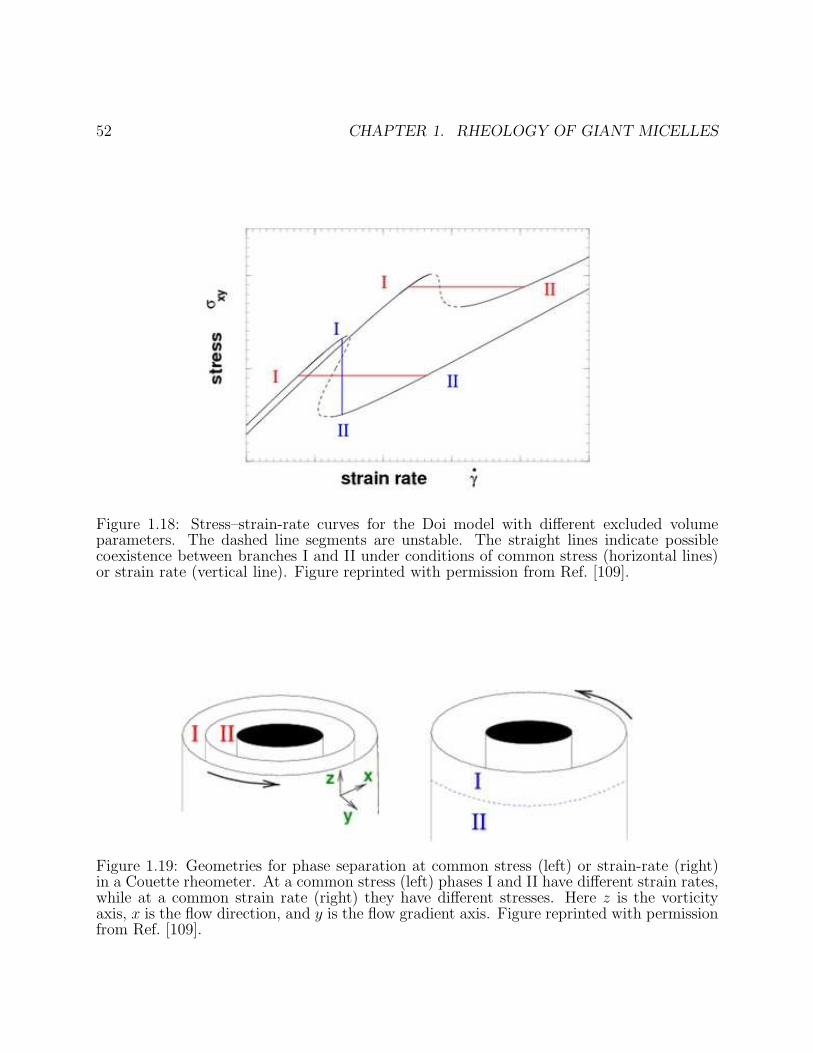
Figure 1.1: Upper panel: Schematic view of aqueous surfactant self-assembly. Lower panel:Schematic phase diagram for self assembly of ionic amphiphiles into giant micelles and relatedstructures. The vertical axis represents volume fraction Φ of amphiphile; the horizontal isthe ratio Cs/C of added salt to amphiphile concentrations. Figure in lower panel from F.Lequeux and S. J. Candau, in Ref. [2], reprinted with permission.


range from somewhat below, to well above, the overlap threshold. This is the region whereviscoelastic (but isotropic) solutions are observed. This regime merits detailed attention fortwo reasons. The first is that micellar viscoelasticity forms the basis of many applications,ranging from personal care products (shampoos) to specialist drilling fluids for oil recov-ery [2]. The second, is that as emphasised first by Rehage and Hoffmann [3], viscoelasticmicelles provide a uniquely convenient laboratory for the study of generic issues in nonlin-ear flow behaviour. This is partly because, unlike polymer solutions (which they otherwiseresemble), the self-assembling character of micellar solutions causes them to self-repair aftereven the most violently nonlinear experiment. (In contrast, strong shearing of conventionalpolymers causes permanent degradation of the chains.) Our focus throughout this review ison rheology, which is the science of flow behaviour. Although we will refer in many placesto experimental data, we make no attempt at a comprehensive survey of the experimentalside of the subject, nor do we describe applications areas in any detail. For an up-to-dateoverview of both these topics, the reader is referred to a recent book [4], of which a shortenedversion of this article forms one Chapter.

We shall address the theoretical rheology of giant micelles at two levels. The first (inSection 1.4) is microscopic modelling, in which one seeks a mechanistic understanding ofrheological behaviour in terms of the explicit dynamics —primarily entanglement and re-versible self-assembly— of the giant micelles themselves. This yields so-called ‘constititiveequations’ which relate the stress in a material to its deformation history. Solution of theseequations for simple experimental flow protocols presents major insights into the fascinat-ing flow properties of viscoelastic surfactant solutions, including near-Maxwellian behaviour(exponential relaxation) in the linear regime, and drastic shear-thinning at higher stresses.These successes mainly concern the strongly entangled region where the micellar solution isviscoelastic at rest; in this regime, strong shear-thinning is usually seen. There are howeverequally strange phenomena occurring at lower concentrations where the quiescent solution isalmost inviscid, but becomes highly viscoelastic after a period of shearing. These will also bediscussed (Section 1.4.6) althought they remain, for the present, much less well understood.

Microscopic models of giant micelles under flow generally treat the micelles as structure-less, flexible, polymer-like objects, albeit (crucially!) ones whose individual identities arenot sustained indefinitely over time. This neglect of chemical detail follows a very successfulprecedent set in the field of polymer dynamics [5, 6]. There, models that contain only fourstatic parameters (persistence length, an excluded volume parameter, the concentration ofchains, and the degree of polymerization or chain length) and two more dynamic ones (afriction constant or solvent viscosity, and the so-called ‘tube diameter’) can explain almostall the observed features of polymeric flows. Indeed, microscopic models of polymer rhe-ology arguably represent one of the major intellectual triumphs of 20th century statisticalphysics [7].

However, at least when extended to micelles, these microscopic constitutive models remaintoo complicated to solve in general flows, particularly when flow instabilities are present.(Such instabilities are sometimes seen in conventional polymer solutions, but appear farmore prevalent in micellar systems.) Moreover, they omit a lot of the important physics,particularly couplings to orientational fields and concentration fluctuations, relevant to theseinstabilities. Therefore we also describe in Section 1.5 some purely macroscopic constitutivemodels, whose inspiration stems from the microscopic ones but which can go much further inaddressing the complex nonlinear flow phenomena seen in giant micelles. These phenomenainclude for example “rheochaos”, in which a steady shear deformation gives chaoticallyvarying stress or vice versa. Our discussion of macroscopic modelling will take us to theedge of current understanding of these exotic rheological phenomena.

1.2. STATISTICAL MECHANICS OF MICELLES IN EQUILIBRIUM 5

Prior to discussing rheology, we give in Section 1.2 a brief survey of the equilibriumstatistical mechanics of micellar self-assembly. More detailed discussions of many of thestatic equilibrium properties of micelles can be found in [4]; we focus only on those aspectsneeded for the subsequent discussion of rheology. Another key component for rheologicalmodelling is the kinetics of micellar ‘reactions’ whereby micelles fragment and/or recombine.These reactions are of course already present in the absence of flow, and represent the kineticpathway whereby equilibrium (for quantities such as the micellar chain-length distribution)is actually reached. We review their properties also in Section 1.2.

In developing the equilibrium statistical mechanics and kinetic theory for giant micelles(Section 1.2), we should keep in mind both the successes and limitations of the rheologicaltheories that come later. Such theories, since their first proposal by one of us in 1987 [8]have had considerable success in predicting the basic features of linear viscoelastic relaxationspectra observed in experiments, and in inter-relating these, for any particular chosen sys-tem, with nonlinear behaviour such as the steady-state dependence of stress on strain rate.These dynamical models take as input the micellar size distribution, stiffness (or persistencelength) and the rate constants for various kinetic processes that cause changes in micellarlength and topology. Such inputs are theoretically well defined, but harder to measure inexperiment. Nonetheless, there are a number of ‘primary’ predictions (such as the shapeof the relexation spectrum, and the inter-relation of linear and nonlinear rheological func-tions; see Section 1.4.3) for which the unknown parameters can either be fully quantified, orelse eliminated. As an aid to experimental comparison, it is of course useful to ask how therheological properties should depend on thermodynamic variables such as surfactant concen-tration, temperature, and salt-levels in the micellar system (Section 1.4.4). But in addressingthese ‘secondary’ issues, the dynamical models can only be as good as our understanding ofhow those thermodynamic variables control the equilibrium micellar size distribution, per-sistence length, and rate constants, as inputs to the dynamical theory. In many cases thisunderstanding is only qualitative, so that these ‘secondary’ experimental tests should not betaken as definitive evidence for or against the basic model.

1.2 Statistical Mechanics of Micelles in Equilibrium

In line with the above remarks, we focus mainly on those aspects of equilibrium self-assemblythat can affect primary rheological predictions. Most of the thermodynamic modelling canbe addressed within mean-field-theory approaches (Sections 1.2.1–1.2.3), although more ad-vanced treatments show various subtleties that still await experimental clarification (Section1.2.4). In Section 1.2.5 we turn to the kinetic question of how micelles exchange materialwith one another within the thermal equilibrium state.

1.2.1 Mean Field Theory: Living Polymers

In typical giant micellar systems the critical micelle concentration (CMC) is low – of order10−4 molar for CTAB/KBr, for example. (CTAB, cetyltrimethylammonium bromide, is awidely studied amphiphile. In what follows, we do not expand the acronyms for this or othersuch materials as their chemical formulas are rarely of interest in our context. KBr is, asusual, potassium bromide, added to alter the head-group interactions.) As concentration is


raised above the CMC, uniaxial elogation occurs and soon micelles become longer than theirpersistence length lp. This is the length over which appreciable bending occurs [5]; oncelonger than this, micelles resemble flexible polymers. Persistence lengths of order 10 - 20 nmare commonplace, though much larger values are possible in highly charged micelles at lowionic strength.

As concentration is increased, there is an onset of viscoelastic behaviour at a volumefraction C usually identified with an ‘overlap’ concentration C∗ for the polymers. (Forproblems with this identification, see 1.2.3 below.) Above C∗, the wormlike micelles are inthe so-called ‘semidilute’ range of concentrations [5] – overlapped and entangled at largedistances, but well separated from one another at scales below ξ, the correlation length or‘mesh size’. In ordinary polymer solutions in good solvents, the behaviour at scales less thanξ is not mean-field-like but described by a scaling theory with anomalous exponents [5]. Wereturn to this in Section 1.2.4, but note that these scaling corrections become small whenthe persistence length of a micellar cylinder is much larger than its diameter, giving modestvalues for a dimensionless ‘excluded volume parameter’ w [5, 6]. Therefore, a mean-fieldapproach – in which excluded volume interactions are averaged across the whole systemrather than treated locally – captures the main phenomena of interest, particularly in theregime of strong viscoelasticity at C ≥ C.

The simplest mean field theory [9,10] assumes that no branch-points and no closed ringsare present (rectified in Sections 1.2.2, 1.2.3), and ascribes a free energy E/2 to each hemi-spherical endcap of a micelle relative to the free energy of the same amount of amphiphilicmaterial residing in the cylindrical body. Denoting by c(N) the number density of aggregatescontaining N amphiphiles or ‘monomers’, the mean field free energy density obeys

βF =∑

N

c(N)[ln c(N) + βE] + F0(φ) (1.1)

Here β = 1/kBT ; the term in E counts two end-caps per chain, and the c ln c piece comesfrom the entropy of mixing of micelles of different lengths. Within a mean-field calcula-tion, these are the only terms sensitive to the size distribution c(N) of the micelles; thefree energy (including configurational entropy) of the cylindrical sections, alongside theirexcluded-volume interactions and all solvent terms, give the additive piece F0(φ) which de-pends only on total volume fraction φ. (It may also depend on ionic strength and relatedfactors.) The volume fraction obeys

φ = v0C = v0

∑

N

Nc(N) (1.2)

where v0 is the molecular volume of the amphiphiles and C their total concentration.

Minimizing (1.1) at fixed φ gives an exponential size distribution

c(N) ∝ exp[−N/N ] ; N ≃ φ1/2 exp[βE/2] (1.3)

The exponential form in each case is a robust result of mean field theory. The φ-dependencein the second equation is also robust (it follows from mass action), but can be treatedseparately from the much stronger exponential factor only so long as parameters like Eand v0 are themselves independent of concentration. (In ionic systems this is a strong andquestionable assumption.) The formula for N as written in (1.3) suppresses prefactoraldependences on v0, lp and a0, where a0 is the cross-sectional area of the micellar cylinders;


these are absorbed into our definition of E. So long as a0 is constant, then exactly the samefunctional forms as in (1.3) control c(L) and L, where L ∝ N is the contour length of amicelle. Within mean field, L in turn controls the typical geometric size R (usually chosenas either the end-to-end distance, or the radius of gyration) of a micelle via R2 ≃ Llp. Thisis the well-known result for gaussian, random-walk chain configurations [5].

We can now work out, within our mean-field approach, the overlap concentration C∗,or overlap volume fraction φ∗ = C∗v0. For a micelle of the typical contour length L wehave R ≃ n1/2lp where n = L/lp is the number of persistence length it contains; this obeysnlpa0/v0 = N . The total volume of amphiphile within the region spanned by this micelle isNv0 and the volume fraction within it therefore φ ≃ Nv0/R

3. At the threshold of overlap,this φ equates to the true value φ∗; then eliminating N via (1.3) gives

C∗v0 = φ∗ ≃ (a0/v1/30 lp)

6/5e−βE/5 (1.4)

For typical cases the dimensionless pre-exponential factor is smaller than unity, but nonethe-less a fairly large E is required if φ∗ is to be below, say 1%. The regime of long, entangledmicelles usually entails scission energies E of around 10 − 20kBT ; in practice, experimentalestimates of φ∗ (best determined by light scattering) are often in the range 0.05–5% [11]. Thescission energy E of course depends on the detailed chemistry of the surfactant moleculesand this (alongside micellar stiffness or persistence length) is one of the main points at whichsuch details enter the theory. Very crudely, one can argue that doubling the mean curvatureof a micellar cylinder to create an end-cap must cost about kBT per molecule in the end-cap region. (If packing energies were much higher than this, one would expect a crystallinerather than fluid packing on the cylinder, which is not typically observed, at least at at roomtemperature.) This gives E ∼ nkBT where n is the number of molecules in two endcaps.Within a factor two, this broadly concurs with the range 10 − 20kBT stated above. Moreprecise theoretical estimates also concur with this range, although values well outside of itare also possible for atypical molecular geometries, e.g. fluorosurfactants [12].

The region around φ∗ is where spectacular shear-thickening rheology occurs (see Section1.4.6). In ionic micellar systems without excess of salt, the strong dependence of lp, E andother parameters on φ itself in this region means that the simple calculations leading to(1.3), and hence the estimate (1.4), are at their least reliable. More detailed theories, whichtreat electrostatic interactions explicitly, give a far stronger dependence of L on φ and alsoa narrower size distribution for the micelles [13]. The overlap threshold φ∗ itself moves tohigher concentration due to the electrostatic tendency to stabilise short micelles.

1.2.2 Role of Branching: Living Networks

The above assumes no branching of micelles. A mean-field theory can in principle be formu-lated to deal with self-assembled micellar networks having arbitrary free energies for bothend caps and branch points [14]. This is, however, somewhat intractable for the generalcase. Fortunately things simplify considerably in the branching-dominated limit; that is,when there are many branch-points per end-cap. For branching via z-fold ‘crosslinks’ (eachof energy Eb) one has, replacing (1.1), the following mean-field result [14]:

βF =∑

N

c(N)[ln c(N) + βEbz−1] + 2(z−1 − 1)C ln(2C) + F0(φ) (1.5)


where C is as defined in (1.2), and c(N) is now the concentration of network strands con-taining N amphiphiles. To understand this result, note that the first logarithmic term isthe translational entropy of a set of disconnected network strands. The second such termestimates the entropy loss on gathering the ends of these strands locally to form z-fold junc-tion points. The term in Eb counts the energy of these junctions and F0(φ) has the samemeaning as in (1.1). The value of z most relevant to micelles is z = 3, since for a systemwhose optimal local packing is a cylinder, a three-fold junction costs less in packing energythan z > 3. Low z is also favoured entropically: to create a four-fold junction one must fusetwo three-fold ones with consequent loss of translational entropy along the network [14].

Minimizing (1.5) to find the equilibrium strand length distribution, one finds this again tobe exponential, with mean strand length L ∼ φ1−z/2 exp[βEb]. This result applies wheneverthe geometric distance between crosslinks, Λ ≃ (Llp)

1/2 greatly exceeds the geometric meshsize ξ, which within mean field theory obeys ξ ∼ a0/φlp. This situation of Λ ≫ ξ iscalled an ‘unsaturated network’ [14] and arises at high enough concentrations (φ ≫ φsat ≃v−10 exp[−βE/(3 − z/2)]). For φ ≤ φsat one has a ‘saturated network’ with Λ ≃ ξ. At low

enough φ this saturated network can show a miscibility gap, where excess solvent is expelledfrom the system rather than increase ξ which would sacrifice branch point entropy [14].

The rheology of living networks (see Section 1.4.5) should differ strongly from the un-branched micellar case. Such a regime has been identified in several systems, primarilycationic surfactants at relatively high ionic strength [15–17]. These accord with the expectedtrend for curvature packing energies: adding salt in these systems stabilizes negatively curvedbranch-points relative to positively curved end-caps [16].

1.2.3 Role of Loop Closure: Living Rings

We have assumed in (1.1) that rings do not arise. A priori, however, there is nothing to stopmicelles forming closed rings. Moreover, for unbreakable polymers (at least) the effect onrheology of closing chains to form rings is thought to be quite drastic [18], so this assumptionmerits detailed scrutiny. It turns out to be satisfactory only when E is not too large, so thatφ∗ in (1.4) lies well above a certain volume fraction φmaxr , defined below, which signifies amaximal role for ring-like micelles.

From (1.4), as E → ∞, the overlap threshold φ∗ for open micelles tends to zero. Inthis limit, there is formally just a single micelle, of macroscopic length. This correspondsto an untenable sacrifice of translational entropy which is easily regained by ring formation.To study this, let us set E → ∞ so that no open chains remain, but allow rings withconcentration cr(N). Then, to replace (1.1), one has [19]

βF =∑

N

cr(N)[ln cr(N) + βfr(N)] + F0(φ) (1.6)

where fr(N) = −kBT ln(Zr), and Zr is the configurational free energy cost of ring closure.Put differently, E − fr(N) is the total free energy cost of hypothetically opening a ring,creating two new endcaps but gaining an entropy kB lnZr. The latter stems both from thenumber of places such a cut could occur, and the extra configurations made available byallowing the chain ends to move apart.

For gaussian (mean-field-like) chains in three dimensions, it is easly shown that Zr =


λN−5/2 [5], where λ is a dimensionless combination (as yet unknown [11]) of a0, v0, lp. Min-imizing (1.6) at fixed φ then gives

cr(N) = λN−5/2eµN (1.7)

where µ is a chemical-potential like quantity. Interestingly, this size distribution for ringsshows a condensation transition. That is, for µ > 0 the volume fraction φr = v0

∑

N Ncr(N)is divergent, whereas for µ ≤ 0 it can apparently be no greater than

φmaxr = λ∞∑

N=Nmin

N−3/2 (1.8)

This limiting value of φr depends not only on λ but on Nmin, which denotes the smallestnumber of amphiphiles that can make a ring-shaped micelle without prohibitive bendingcost. (Such a micelle must presumably have contour length of a few times lp.)

This mathematical situation, in which there is an apparently unphysical ‘ceiling’ φmaxr < 1on the total volume fraction of rings a system can contain, is reminiscent of Bose condensation[20]. It represents the following physical picture, valid in the E → ∞ limit. For φ ≤ φmax

rone has the power law distribution of ring sizes in (1.7), cut off at large N by an exponentialmultiplier (resulting from small negative µ). For φ > φmaxr , one has a pure power lawdistribution of rings, in which total volume fraction φmaxr resides; plus an excess volumefraction φ− φmaxr which exists as a single ‘giant ring’ of macroscopic length. This giant ringis called the condensate; its sudden formation at φ = φmaxr represents a true phase transition.

Obviously, an infinite ring is possible only because the limit E → ∞ was taken; for anyfinite E, all rings with N > N as defined in (1.3), including the condensate, will break upinto pieces (roughly of size N). Indeed, if E is finite one can, within mean-field theory,simply add the chain and ring free energy contributions as

βF =∑

N

c(N)[ln c(N) + βE] +∑

N

cr(N)[ln cr(N) + βfr(N)] + F0(φ) (1.9)

From this one can prove that the condensation transition is smoothed out for any E < ∞[21]. Nonetheless, if E is large enough that the overlap threshold φ∗(E) obeying (1.4)falls below φmaxr obeying (1.8), then the condensation transition of rings, though somewhatrounded, should still have detectable experimental consequences. These should mainly affecta (roughly) factor-two window in concentration either side of φmaxr . For φ≪ φmaxr there areno very large rings and hence limited opportunities for viscoelasticity. For φ ≫ φmaxr thevolume fraction φ− φr of long chains exceeds that of rings, and the chains dominate.

Because of uncertainty over the values of λ and Nmin in (1.8) and how these might dependon chain stiffness, ionic strength, etc., φmaxr is one of the least well-charactarized of all staticquantities for giant micelles. In fact, there is relatively little (but some [22]) experimentalevidence for a ring-dominated regime in any micellar system, suggesting perhaps that, forreasons as yet unclear, φmaxr lies well below the range of φ accessed in most experiments.However, as outlined in Section 1.4.6 below, a ring-dominated regime might explain some ofthe strangest of all the rheological data in the shear-thickening regime just below C [23].

Note that in an earlier review (Ref. [11]) an impression was perhaps given that ring-formation matters only within scaling theories (discussed next) but not at the mean-fieldlevel. This is true only if φmaxr is indeed small; in that case rings will only matter for very


large E, and micelles are of sufficient size that excluded volume effects, even if locally weak,are likely to give scaling corrections to mean-field. However, rings are not purely a scalingphenomenon: even in a strictly mean-field picture, φmaxr is a well-defined quantity at whicha ring-condensation phase transition arises in the limit of large E.

1.2.4 Beyond Mean Field Theory

As with conventional polymers [5], micelles can exhibit non-gaussian statistics, induced byexcluded-volume interactions arising from the inability of two different sections of the micelleto occupy the same spatial position. In principle, this gives scaling corrections to all thepreceding mean-field results, altering the various power law exponents that appear in equa-tions such as (1.3,1.7). As mentioned previously, however, micelles often have a persistencelength lp large compared to their cross-section and therefore tend to have relatively weakexcluded volume interactions. Therefore, giant micellar systems can often be expected to liein a messy crossover region between mean-field and the scaling theory. For completeless weoutline the scaling results here (see [11, 14, 24] for more details), but without attempting totrack dependences on parameters like lp, a0, v0.

First, consider a system with no branches or rings. In such a system, the excluded volumeexponent ν ∼ 0.588 governs the non-gaussian behaviour of a self-avoiding chain; R ∼ Lν [5].This gives ξ ∼ φν/(1−νd) ∼ φ−0.77 where d = 3 (the dimension of space). This leads to a scalingof the transient elastic modulus G0 (defined in Section 1.4 below): βG0 ∼ ξ−d ∼ φ2.3, whichis proportional to the osmotic pressure Π [5]. This differs from the simplest mean-field-typeestimate which has G0 ∼ Π ∼ φ2. Second, one finds in place of (1.3)

c(L) ∝ exp[−L/L] ; L ≃ φy exp[βE/2] (1.10)

where y = [1 + (γ − 1)/(νd − 1)]/2 ≃ 0.6; here γ ≃ 1.2 is another standard polymerexponent [5]. In practice this is rather a modest shift from the result in (1.3).

In the presence of branch points, the important case remains z = 3. Here the mean fieldresult for the mean network strand length L ∼ φ−1/2 exp[βE] becomes L ∼ φ−∆ exp[βE]with an exponent ∆ ∼ 0.74; the expression for ∆ in terms of standard polymer exponentsis given in Ref. [14]. Similarly the mean-field result φsat ∼ e−2βE/3 becomes φsat ∼ e−βE/y

with y ∼ 0.56 [14]. Note that there is still the possibility of phase separation between asaturated network and excess solvent, even under good solvent conditions – and there issome experimental evidence for exactly this phenomenon [17].

Scaling theories in the presence of rings become even more complicated [19]; even theexponent ν, governing the local chain geometry, is slightly different in the ring dominatedregime [24]. Near φmaxr (which has the same meaning as before, but no longer obeys (1.8))there is a power-law cascade of rings, controlled by a distribution similar to (1.7), but with asomewhat larger exponent (2.74 instead of 5/2) [24]. This cascade of rings creates ‘power lawscreening’ of excluded volume interactions [25], causing ν to shift very slightly downward [19].Perhaps fortunately in view of these complications, the ring-dominated regime, if it existsat all, is poorly enough quantified experimentally that comparison with mean field theory isall that can be attempted at present.


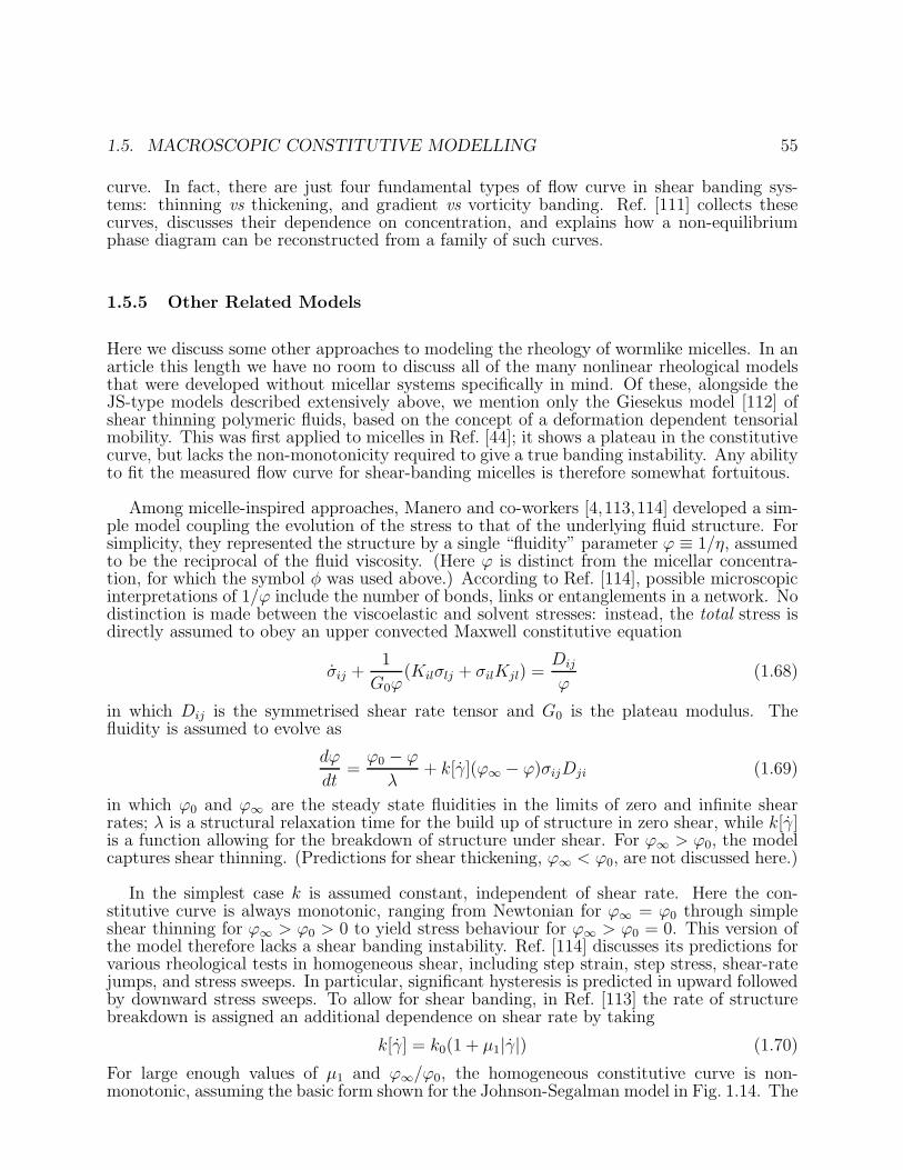
Figure 1.2: The three main types of micellar reaction: Top, reversible scission; middle, endinterchange; bottom, bond interchange

1.2.5 Reaction Kinetics in Equilibrium

Alongside the micellar length distributions addressed above, a key ingredient into rheologicalmodelling is the presence of reversible aggregation and disaggregation processes (which weshall call micellar ‘reactions’), allowing micelles to exchange material. We will treat thesereactions at the mean-field level, in which micelles are ‘well-mixed’ at all times (so thereis no correlation between one reaction and the next). Our excuse for this simplificationis that, although deviations from mean-field theory are undoubtedly important in somecircumstances and have been worked out in detail theoretically [26], there is so far rather littleevidence that this matters in the strongly entangled regime (C ≥ C) where viscoelasticity

is primarily seen. And, although in the shear thickening region (C ≃ C) it is quite possiblethat non-mean-field kinetic effects become important, there is so much else that we do notunderstand about this regime (Section 1.4.6) that a detailed discussion of correlated reactioneffects would appear premature.

We neglect branching and ring-formation in the first instance, and also distinguish reac-tions that change the aggregation number of a particular micelle N by a small increment,∆N ≃ 1, from those which create changes ∆N of order N itself. The former reactions can ofcourse lead to significant changes in micellar size over time, but as N increases, the timescalerequired for this gets longer and longer [27]. Unless the reaction rates for all reactions of thesecond (∆N ≃ N) type are extremely slow, these latter will dominate for large aggregates.From now on, we consider only reactions with ∆N ≃ N , of which there are three basic types:reversible scission, end-interchange, and bond-interchange, as shown in Figure 1.2.

In reversible scission, a chain of length L breaks spontaneously into two fragments of sizeL′ and L′′ = L − L′. (Note that the conservation law N ′′ + N ′ = N really applies to Nand not L as written here; but if we ignore the minor corrections to L represented by thepresence of end-caps, the sum of micellar lengths is also conserved.) In thermal equilibriumthe reverse process (end-to-end fusion) happens with exactly equal frequency; this followsfrom the principle of detailed balance [28]. If, for simplicity, we assume that the fusion rateof chains of lengths L and L′ is directly proportional to the product of their concentrations,then the fact that detailed balance holds for the equilibrium distribution (1.3) can be used


to reduce the full kinetic equations (as detailed, e.g., in Ref. [8]) to a single rate constantkrs. This is the rate of scission per unit length of micelle, and is independent of both theposition within, and the length of, the micelle involved [8]. More relevant physically is

τrs = (krsL)−1 (1.11)

which is the time taken for a chain of the mean length to break into two pieces by a re-versible scission process. Note that, by detailed balance, the lifetime of a chain-end beforerecombination is also τrs [8]. Moreover, solution of the full mean-field kinetic equations [29]shows that if L is perturbed from equilibrium, for example by a small jump in temperature(T-jump), L relaxes monoexponentially to equilibrium with a decay time τrs/2. (In fact thisapplies not only to L but to the entire perturbation to the micellar size distribution, whichfor this form of disturbance is an eigenmode of the kinetic equations [29].) The response toa nonlinear, large amplitude jump is also calculable [30]. These results allow τrs to be esti-mated from T-jump data [31], providing an important constraint on the rheological modelsof Section 1.4.

Turning to end-interchange, this is the process where a ‘reactive’ chain-end bites intoanother micelle, carrying away part of it (Figure 1.2). Assuming all ends to be equallyreactive, and applying detailed balance, one finds that all points on all micelles are equallylikely to be attacked in this way. There is, once again, a single rate constant kei, but nowthe lifetime of any individual chain end is 1/keiφ, since the availability of places to bite intois proportional to φ. The lifetime of a micelle of the average length, before it is involved inan end-interchange reaction of some sort, is [29]

τei = (4keiφ)−1 (1.12)

In contrast to the reversible scission case, analysis of the full mean-field kinetic equations [29]shows that end-interchange is invisible in T-jump: for the specific form of perturbation thatarises there, no relaxation whatever occurs by this mechanism. Beyond mean-field kineticsthis would no longer hold, but there remains an important limitation to end-interchange inbringing the system to equilibrium. Specifically, end-interchange conserves the total numberof micelles. Accordingly if a disturbance, whether rheological or thermal in origin, is appliedthat perturbs the total chain number

∑

N c(N) away from equilibrium, this will not fullyrelax until the time-scale τrs is attained, even if this is much larger than τei [29]. In the meantime, the end-interchange process relaxes the size distribution c(N) towards the exponentialform c(N) ∝ exp[−N/N ] of (1.3); but with a nonequilibrium value of N . This separationof time scales may lie at the origin of strange ‘structural memory’ effects seen in certainsystems (Section 1.4.8 below) [23].

Note that since in our simple models the micellar energy is fixed by the number of end caps,conservation of micellar number in end-interchange reactions (and also bond-interchange,below) is tantamount to conservation of the total energy stored in such end caps. Anenergy-conserving processes cannot, unaided, relax a system after a jump in temperature.However, since E is really a free energy and the dynamics is not microcanonical, conservationof micellar number is perhaps the more fundamental concept in distinguishing interchangefrom reversible scission kinetics; in subsequent discussions, we take this view.

Finally we turn to the bond-interchange process [32] in which micelles transiently fuseto form a four-fold link before splitting again into differently connected components (Figure1.2). This process, like end-interchange, conserves chain number. Indeed it does not evenalter the identity of chain ends. Since, in entangled polymeric systems, stress relaxation oc-curs primarily at the chain ends, bond-interchange is far less effective than reversible scission


or end-interchange in speeding up the disentanglement of micelles (see Section 1.4). In fact,although a breaking time τbi = (kbiLφ)−1 can be defined, this enters the rheological modelsdifferently from τrs or τbi (Section 1.4.2 below). Bond interchange also allows chains to effec-tively pass through one another by decay of the four-fold intermediate, creating a somewhatdifferent relaxation channel for chain disentanglement and stress relaxation [33]. However(as previously discussed in Section 1.2.2) a transient four-fold link is likely to dissociaterapidly into two three-fold links. Such three-fold links are in turn the transition states of theend-interchange process. If these links disconnect rapidly, then the end-interchange process(which their decay represents) is probably dominant over bond interchange. If they do notdecay rapidly, then it is likely that their existence cannot be ignored for static purposes; onehas a branched system in equilibrium (see Section 1.2.2).

The reaction kinetics in branched micellar networks is far from easy to cast in terms ofsimple mean-field reaction equations, as studied, e.g., in Ref. [29] for unbranched chains.However, within such a network, alongside any bond-interchange reactions that are present,structural relaxation can still occur by reversible scission or end-interchange of a section ofthe micellar network between junctions. Time-scales τrs or τei can then be defined as thelifetime of a typical network strand before destruction by such a process. In the reversiblescission case (1.11) still holds, now with L the mean strand length in the network [15].

In the presence of rings, the three reaction schemes of Figure 1.2 remain applicable inprinciple. It is then notable that the chain number

∑

N c(N), though not the ring number∑

N cr(N), is still conserved by the two interchange processes. Whenever open chains arepresent, reversible scission is needed for them to reach full thermal equilibrium [23].

1.2.6 Parameter Variations

As stated previously, the static mean-field theories given above (in Sections 1.2.1 – 1.2.3)take as their parameters E, lp, a0, v0. Also relevant is the excluded volume parameter w [5,6].This controls the strength of repulsions between sections of micelle; for hard core interactionsthis is a function of lp and a0, but in general w also depends on all local interaction forcesbetween sections of micelles. Nonetheless, within mean-field, this parameter only affects thepurely φ-dependent term F0(φ) in (1.1, 1.5, 1.6) and hence has no effect on the mean micellarlength L or the size distribution c(L). (The most important role of w is, in fact, to controlthe crossover to the scaling results discussed in Section 1.2.4 above.) All of the parametersE, lp, a0, w in principle can have explicit dependence on the volume fraction φ. This certainlyoccurs in ionic micellar systems at low added salt, where the ionic strength depends stronglyon φ itself and modulates directly parameters such as E and lp. Ion-binding and similareffects can also be strongly temperature dependent. Similar remarks apply to the reactionrate constants krs, kei considered in Section 1.2.5 above, and hence also to their activationenergies EA ≡ −∂ ln k/∂β. The rheological consequences of these parameter variations arediscussed in Section 1.4.4.


1.3 Theoretical Rheology

Since microscopic models for giant micelle rheology draw strongly from earlier progress inmodelling conventional polymers, we review that progress briefly here. (See [6] for a definitiveaccount.) In doing so we can also establish some of the concepts and terms used in rheology– a field which remains regrettably foreign to the majority of physics graduates.

1.3.1 Basic Ideas

Rheology is the measurement and prediction of flow behaviour. The basic experimentaltool is a rheometer – a device for applying a controlled stress to a sample and measuringits deformation, or vice versa. However, in recent years a variety of rheophysical probes,which allow simultaneous microscopic characterisation or imaging, have been developed [34,35]. For the complex flows that can arise in giant micelles, these enhanced probes offerimportant additional information about how microstructure and deformation interact. Manyrheometers use a Couette cell, comprising two concentric cylinders, of radius r and r + hwith the inner one rotating. (See Figure 1.19 below for an illustration of this geometry.)Others use a cone-plate cell (Figure 1.3) where a rotating cone contacts a stationary plateat its apex, with opening angle θ. In the limit of small h/r or small θ, each device resultsin a uniform stress in steady state; in each case, the shear stress can be measured from thetorque. Some cone-and plate devices can also measure ‘normal stress differences’ definedbelow.

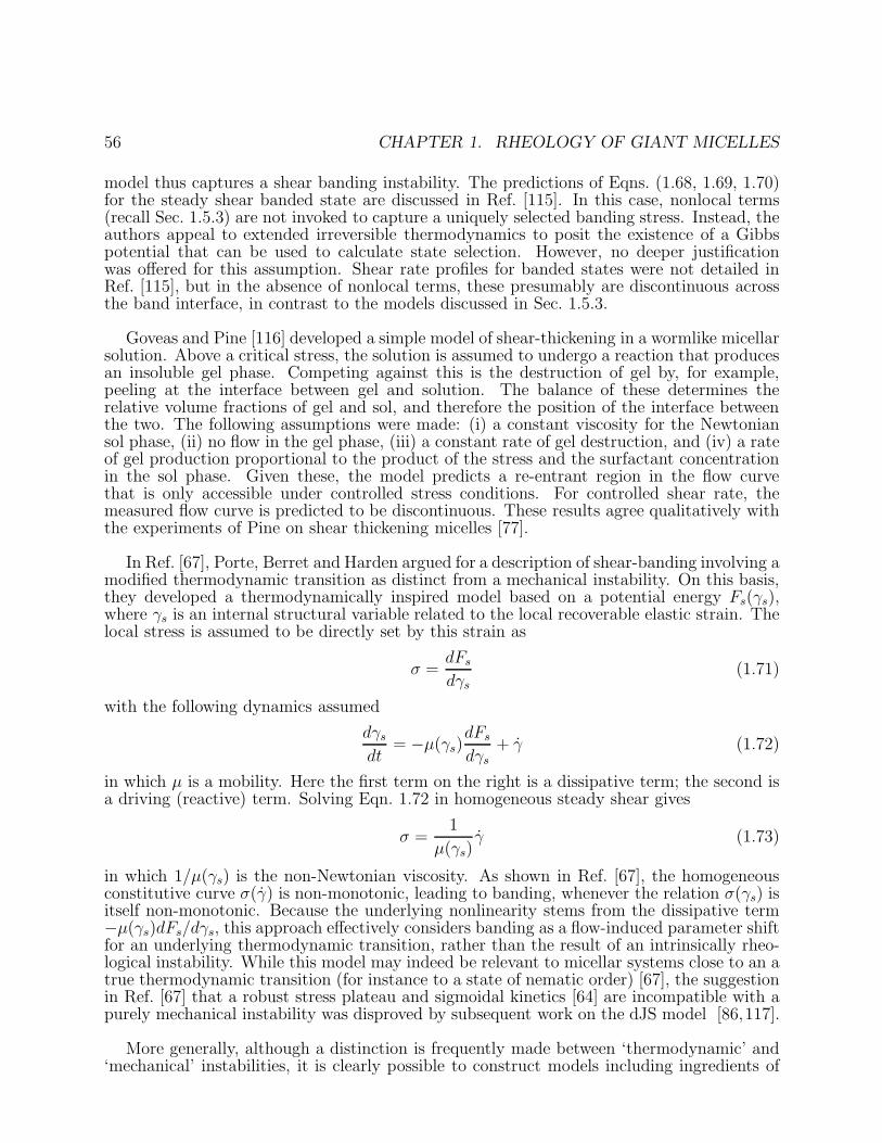
Figure 1.3: A cone-plate rheometer. The sample (black) sits between a rotating cone (white)and a solid plate (grey).

Statistical Mechanics of Stress

We shall use suffix notation, with roman indices and the usual summation convention, forvectors and tensors; letters a...w can therefore stand for any of the three cartesian directions

1.3. THEORETICAL RHEOLOGY 15

x, y, z. Greek indices will be reserved for labels of other kinds.

Consider a surface element of area dA with unit normal vector ni. Denote by dFi theforce acting on the interior of the surface element caused by what is outside. If ni is reversed(switching the definitions of interior and exterior), then so is Fi; this accords with Newton’sthird law. Writing the usual vectorial area element as dSi = nidA, we have

dFi = σijdSj (1.13)

which defines the stress tensor σij . This tensor is symmetric. The hydrostatic pressureis defined via the trace of the stress tensor, as p = −σii/3; what matters in rheology the(traceless) ‘deviatoric’ stress σdev

ij = σij + pδij . This includes all shear stresses, and also twocombinations of the diagonal elements, usually chosen as the two normal stress differences,

N1 = σxx − σyy ; N2 = σyy − σzz (1.14)

For simplicity we assume pairwise interactions between particles. (The choice of what we

define as a particle is clarified later.) The force fαβi exerted by particle α on particle β then

depends on their relative coordinate rαβi (measured by convention from α to β). But this pairof particles contributes to the force dFi acting across a surface element dSi only if the surfacedivides one particle from the other. The probability of this happening is dSir

αβi /V where V

is the volume of the system. (This is easiest seen for a cubic box of side L with a planardividing surface of area A = L2 with normal ni along a symmetry axis; Figure 1.4). The

separation of the particles normal to the surface is clearly ℓ = rαβi ni, and the probability

of their lying one either side of it is then just ℓ/L, which can be written as Arαβi ni/V .

Accordingly, the total force across a surface element dSi is dFi = −∑

αβ dA(rαβj nj)fαβi /V

which by definition acts outward (hence the minus sign). Bearing in mind (1.13), this gives

σij = −V −1∑

αβ

rαβi fαβj = −ρ2V 〈rifj〉 (1.15)

where the average is taken over pairs and ρ is the mean particle density.

Figure 1.4: Contribution from a polymer ‘subchain’ to the stress tensor. The endpoints ofthe chain can be viewed as two particles, with the chain in between supplying a ‘spring force’between them.


An example is shown in Figure 1.4, where a polymer ‘subchain’ is shown crossing thesurface. At a microscopic level, one could choose the individual monomers as the particles,and their covalent, van der Waals, and other interactions as the forces in (1.15). (This is

often done in computer simulation [36,37].) But so long as the force fαβi is suitably redefinedas an effective, coarse grained force that includes entropic contributions, we can equally wellconsider a polymer chain as a sparse string of ‘beads’ connected by ‘springs’. At this largerscale, the interaction force fαβi has a universal and simple dependence on rαβi , deriving froman ‘entropic potential’ U(ri) = (3kBT/2b

2)riri, where b2 ≡ 〈riri〉. This is a consequence ofthe well-known gaussian distribution law for random walks, of which the polymer, at thislevel of description, is an example. The entropic potential is defined so that the probabilitydistribution for the end-to-end vector of the subchain obeys P (ri) ∝ exp[−U(ri)/kBT ]; thisform identifies U as the free energy. The force now obeys

fαβi = −dU(rαβi )/drαβi = −(3kBT/b2)rαβi (1.16)

which gives, using (1.15), the polymeric contribution to the stress tensor:

σpolij =

Nspr

V

3kBT

b2〈rirj〉 (1.17)

Here the average is over the probability distribution P (ri) for the end-to-end vectors of ourpolymeric subchains (or springs); Nspr/V is the number of these per unit volume. In polymermelts, contributions such as the one we just calculated completely dominate the deviatoricstress. In solutions there may also be a significant contribution from local viscous dissipationin the solvent. In this case, although a formula such as (1.15) still holds in principle, it ismore convenient to work with (1.17) and add a separate solvent contribution directly to thestress tensor. For a Newtonian solvent, the additional contribution is σsol

ij = ηsol(Kij +Kji),where Kij is the velocity gradient tensor introduced below.

Strain and Strain Rate

Consider a uniform, but possibly large, deformation of a material to a strained from anunstrained state. The position vector ri of a material point is thereby transformed into r′i;the deformation tensor Eij is defined by r′i = Eijrj . For small deformations, one can writethis as Eij = δij + eij so that the displacement ui = r′i − ri obeys ui = eijrj. Alternativelywe may write this as eij = ∇jui. Consider now a time-dependent strain, for which vi ≡ uidefines the fluid velocity, which depends on the position ri. We define the velocity gradienttensor Kij = ∇jvi = eij ; this is also sometimes known as the ‘rate of strain tensor’ or‘deformation rate tensor’. If we now consider a small strain increment, eijδt,

ri(t+ δt) = (δij + eijδt) rj(t) (1.18)

The left hand side of this is, by definition, Eij(t+ δt)ri(0) where the time-dependent defor-mation tensor Eij(t) connects coordinates at time zero with those at time t. Inserting also

rj(t) = Ejk(t)rk(0) we obtain Eij = KikEkj, or equivalently

∂Eij/∂t = eikEkj (1.19)

An important example is simple shear. Consider a shear rate γ with flow velocity alongx and its gradient along y: then vi = γyδix. The velocity gradient tensor is Kij = γδixδjy,


that is, Kij is a matrix with γ in the xy position and all other entries zero. Solving (1.19)for arbitrary γ(t) then gives Ett′

ij = δij +γ(t, t′)δixδjy where Ett′

ij is defined as the deformation

tensor connecting vectors at time t to those at time t′, and γ(t, t′) =∫ t′

t γ(t′′)dt′′ is the total

strain between these two times.

1.3.2 Linear Rheology

Linear rheology addresses the response of systems to small stresses. Imagine an undeformedblock of material which is suddenly subjected, at time t1, to a small shear strain γ. Taking thedisplacement along x and its gradient along y, we then have for the resulting deformationtensor Eij = δij + γδixδjy. Suppose we measure the corresponding stress tensor σij(t).Linearity, combined with time-translational invariance of material properties, requires that

σyx = σxy = G(t− t1)γ (1.20)

and that all other deviatoric components of σij vanish, at linear order in γ, by symmetry.(For example, N1(γ) = N1(−γ), which requires N1 = O(γ2).) This defines the linear step-strain response function G(t). This function is zero for t < 0; it is discontinuous at t = 0,jumping to an initial value which is very large (on a scale set by G0, defined below). Thislargeness reflects the role of microscopic degrees of freedom; there follows a very rapid decayto a more modest level arising from mesoscopic (polymeric) degrees of freedom. In mostcases this level persists for a while, making it useful to identify it as G0, the transient elasticmodulus. (In models that ignore microscopics, one can identify G0 = G(t → 0+).) On thetimescale of mesoscopic relaxations, which are responsible for viscoelasticity, G(t) then fallsfurther.

Now suppose we apply a time-dependent, but small, shear strain γ(t). By linearity, wecan decompose this into a series of infinitesimal steps of magnitude γ(t′)dt′; the response tosuch a step is dσxy(t) = G(t− t′)γ(t′)dt′. We may sum these incremental responses, giving

σxy(t) =∫ t

−∞

G(t− t′)γ(t′)dt′ (1.21)

where, to allow for any displacements that took place before t = 0, we have extended theintegral into the indefinite past. Hence G(t) is the memory kernel giving the linear stressresponse to an arbitrary shear rate history. This is an example of a constitutive equation.However, the constitutive equation for nonlinear flows is far more complicated.

In steady shear γ(t) is constant; therefore from (1.21) one has σxy(t) = γ∫ t−∞

G(t− t′)dt′.However, the definition of a fluid’s linear viscosity (its ‘zero-shear viscosity’, η) is the ratioof shear stress to strain rate in a steady measurement when both are small; hence

η =∫

∞

0G(t)dt = lim

ω→0[G∗(ω)/iω] . (1.22)

This is finite so long as G(t) decays to zero faster than 1/t at late times, which is true in allviscoelastic liquids (as opposed to solid-like materials), including giant micelles.


Oscillatory Flow; Linear Creep

The case of an oscillatory flow is often studied. We write γ(t) = γ0eiωt (taking the real part

whenever appropriate); substituting in (1.21) gives after trivial manipulation

σxy(t) = γ0eiωtG∗(ω) (1.23)

where G∗(ω) ≡ iω∫

∞

0 G(t)e−iωtdt; this is called the complex modulus. The complex modulus,or ‘viscoelastic spectrum’, is conventionally written G∗(ω) = G′(ω) + iG′′(ω) where the realquantities G′ and G′′ are respectively the in-phase or elastic response, and the out-of-phaseor dissipative response. (These are called the ‘storage modulus’ and the ‘loss modulus’respectively.) Many polymeric fluids exhibit a ‘longest relaxation time’ τ in the sense thatfor large enough t, the relaxation modulus G(t) falls off asymptotically like exp[−t/τ ]. In thiscase one has at low frequencies G′ ∼ ω2 and G′′ ∼ ω. For polymer melts and concentratedsolutions, as frequency is raised G′ passes through a plateau whereas G′′ starts to fall;eventually at high frequencies both rise again. This is sketched in Figure 1.5 where, as iscommon practice, a double logarithmic scale is used to plot the viscoelastic spectra.

Figure 1.5: Artist’s impression of the viscoelastic spectrum for a typical polymeric material;the storage and loss moduli G′(ω), G′′(ω) are solid and dotted lines respectively.

One can also study the steady-state flow response to an oscillatory stress. This defines afrequency-dependent complex compliance J∗(ω); however, within the linear response regimethis is just the reciprocal of G∗(ω). Suppose, instead of applying a step strain as was usedto define G(t) in (1.20), we apply a small step in shear stress of magnitude σ0 and measurethe strain response γ(t). This defines a compliance function γ(t)/σ0 = J(t) which is thefunctional inverse of G(t) (that is,

∫

J(t)G(t− t′)dt = δ(t′)). To see this, one can repeat thederivation of (1.23) with stress and strain interchanged, to find that J∗(ω) = iω

∫

J(t)e−iωtdt.For a viscoelastic liquid γ(t) rises smoothly from zero, and the system eventually asymptotesto a steady flow: γ(t → ∞) = σ0(t/η + J (0)

e ). The offset J (0)e , measured by extrapolating

the asymptote back to the origin, is called the steady-state compliance. It can be written asJ (0)e =

∫

∞

0 tG(t)dt/η2 and is therefore more sensitive to the late-time part of G(t) than theviscosity η =

∫

∞

0 G(t)dt.


The Linear Maxwell Model

The simplest imaginable G(t) takes the form G(t) = G0 exp(−t/τM ) for all t > 0 and iscalled the linear Maxwell model, after its inventor James Clerk Maxwell. G0 is a transientelastic modulus and τM a relaxation time (in this model, it is the only such time) called theMaxwell time. The viscosity is η = G0τM ; note that a Newtonian fluid is recovered by takingG0 → ∞ and τM → 0 at fixed η. In nature, nothing exists that is quite as simple as theMaxwell model: but the low-frequency linear viscoelasticity of certain giant micellar systemsis remarkably close to it (Figure 1.6). The viscoelastic spectrum of the Maxwell modelis G∗(ω) = G0iωτM/(1 + iωτM) whose real and imaginary parts closely resemble Figure1.6: a symmetric maximum in G′′ on log-log through which G′ passes as it rises towardsa plateau. This is distinct from ordinary polymers, where the peak is lopsided (with slopecloser to −1/2 on the high ω side), with G′ not passing through the maximum (Figure 1.5).Understanding the near-Maxwellian behaviour of giant micelles in linear rheology is one ofthe main achievements of the ‘reptation-reaction’ models outlined in Section 1.4 below.

Figure 1.6: Viscoelastic spectrum for a system of entangled micelles: arguably nature’sclosest approach to the linear Maxwell model, for which the peak inG′′ is perfectly symmetricand G′ crosses through this peak at the maximum. Figure reprinted with permission fromRef. [38].

1.3.3 Linear Viscoelasticity of Polymers: Tube Models

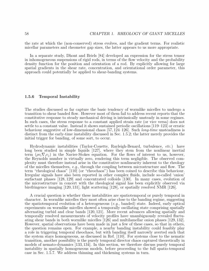
Figure 1.7 shows a flexible polymer. The chain conformation is a random walk; its end-to-endvector is gaussian distributed. In both polymeric and micellar systems there are correctionsto gaussian statistics arising from excluded volume effects at length scales smaller than thestatic correlation length ξ. These effects are screened out at larger distances [5], and theireffects in micelles anyway limited (see Section 1.2.4); we ignore them here.

Dense polymers are somewhat like an entangled mass of spaghetti, lubricated by Brownianmotion. The presence of other chains strongly impedes the thermal motion of any particularchain. Suppose for a moment that the ends of that chain are held fixed. In this case, theeffect of the obstacles can be represented as a tube (Figure 1.7 A). Because it wraps arounda random walk, the tube is also a random walk; its number of steps NT and step-length b


Figure 1.7: A polymer chain (light line). Surrounding chains present obstacles that the chaincannot cross. These can be modelled by a tube (heavy line). The stress relaxation responseafter step strain is controlled by the fraction of the intial tube still occupied by the chainat time t. Frames A-D show the state of the tube at four consecutive times, with vacatedregions shown dotted. Although the emerging chain creates new tube around itself (notshown) this part is assumed to be created in the strained environment, and hence carries noshear stress.


(comparable to the tube diameter) must obey the usual relation 〈R2〉 = NT b2 where R is

the end-to-end distance of both the tube and the chain. This distance can be measured byscattering with selected labelling, as can, in effect, the tube diameter (or step length), bylooking at fluctuations in chain position on short enough timescales that the chain ends don’tmove much. However, there is no fundamental theory that can predict b; in what follows itis a parameter. It is quite large, so that chains smaller than a few hundred monomers donot feel the tube at all. (The largeness of b remains an active topic of research [39].) Inwhat follows we will address strongly entangled materials for which NT ≫ 1, ignoring manysubtle questions that arise when NT is of order unity.

Suppose we now take a dense polymer system and perform a sudden step-strain with shearstrain γ. The chain will instantaneously deform with the applied strain. Since a deformedrandom walk is not maximally random, but biased, this causes a drop in its configurationalentropy. Quite rapidly, though, degrees of freedom at short scales (within the tube) canrelax by Brownian motion. Once this has happened, the only remaining bias is at the scaleof the tube: the residual entropy change ∆S of the chain is effectively that of the tube inwhich it resides. A calculation [6] of the entropy of deformed random walks gives a resultingfree energy change

∆F = −T∆S =1

2G0γ

2 (1.24)

where we identify G0 as the transient elastic modulus; this comes out as G0 = 4kBTn/5where n is the number of tube segments per unit volume. Hence the elastic modulus is closeto, but not exactly, kBT per tube segment.

What happens next? The chain continues to move by Brownian motion, as do its neigh-bours. Although the individual constraints may come and go to some extent, the primaryeffect is as if the chain remains hemmed in by its tube (Figure 1.7). Therefore it can diffuseonly along the axis of the tube (curvilinear diffusion). The curvilinear diffusion constant Dc

is inversely proportional to chain length L [5]. Curvilinear diffusion allows a chain to escapethrough the ends of the tube. When it does so, the chain encounters new obstacles and,in effect, creates new tube around itself. However, we assume that this new tube, which iscreated at random after the original strain was applied, is undeformed. This turns out tobe a very good approximation, mainly since b is so large: the deformation at the tube scaleleads to a local, molecular level alignment that is very small indeed. (Such an alignmentmight ‘steer’ the emerging chain end so that new tube was correlated with the old; this effectis measurable [40], but negligible for our purposes.) This causes the stored free energy ∆Fto decay away as ∆F = G(t)γ2/2 where

G(t) = G0µ(t) (1.25)

Here we identify µ(t) as the fraction of the original tube (created at time zero) which isstill occupied, by any part of the chain, at time t. (In Figure 1.7, this part of the tubeis shown with the solid line in each time frame; the remaining, vacated, regions are showndotted.) The problem of finding µ(t) can be recast [5] as the problem of finding the survivalprobability up to time t of a particle of diffusivity Dc which lives on a line segment (0, L),with absorbing boundary conditions at each end; the particle is placed at random on the linesegment at time zero. To understand this, choose a random segment of the initial tube andpaint it red; then go into a frame where the chain is stationary and the tube is moving. Thered tube segment, which started at a random place, diffuses relative to the chain and is lostwhen it meets a chain end. This tube segment is our particle, and its survival probabilitydefines µ(t).


It is remarkable that the tube concept simplifies our dynamics from a complicated many-chain problem, first into a one-chain (+tube) problem, and then into a one-particle problem.The result of this calculation, a good revision exercise in eigenfunction analysis [6], is:

µ(t) =∑

n=odd

8

n2π2exp

[

−n2t/τR]

(1.26)

where τR = L2π−2/Dc. This parameter is called the ‘reptation time’ (‘reptate’ means tomove like a snake through long grass), and sets the basic timescale for escape from the tube.The calculated µ(t) is dominated by the slowest decaying term – hence it is not that far fromthe Maxwell model, though clearly different from it, and resembles the left part of Figure1.5. (To understand the upturn at the right hand side of that figure, one needs to includeintra-tube modes; see [6].) From this form of µ(t) follow several results: for example theviscosity is η =

∫

G(t)dt = G0τrπ2/12 and the steady-state compliance obeys J (0)

e G0 = 6/5.Thus the tube model gives quantitative inter-relations between observable quantities, andthe number of these relations significantly exceeds the number of free parameters in thetheory — which can be chosen, in effect, as G0 and a diffusivity parameter Dc = DcL.

The model predicts that η = G0L3/(12Dc); since G0 is independent of molecular weight,

η at fixed φ varies as L3 for long chains. The experiments lie closer to η ∼ L3.4, at leastfor modest L, but with a prefactor such that the observations lie below the tube model’sprediction until extremely large L is attained (at which point, in fact, the data bend overtowards L3). This viscosity deficit at intermediate chain lengths has, in recent years, beensuccessfully accounted for by studying more closely the role of intra-tube fluctuation modesand their effects on other chains; see [41].

1.3.4 Nonlinear Rheology

Nonlinear rheology addresses the response of a system to finite or large stresses. In theabsence of a superposition principle, such as the one that holds for linear response, therange of independent measurements is much wider. Nonlinear versions exist of the step-strain and step-stress response measurements discussed in Section 1.3.2, and of oscillatorymeasurements in which either stress or strain oscillate sinusoidally (though in the nonlinearregime, the induced strain or stress will have a more complicated waveform).

In nonlinear step strain, a deformation Eij = δij + γδixδjy is suddenly applied at time t1,just as in Section 1.3.2, but now γ need not be small. Analogous to (1.20) we define

σxy = G(t− t1; γ)γ (1.27)

where a factor of γ ensures that G(t− t1; 0) = G(t− t1) (so the small-strain limit coincideswith the linear modulus defined previously). A system is called ‘factorable’ if G(t− t1; γ) =G(t− t1)h(γ), but this is not the general case. Whereas at linear order all other deviatoriccomponents of σij vanished by symmetry, in the nonlinear regime one can expect to measurefinite normal stress differences N1, N2, as defined in (1.14). In some cases, including manysystems containing giant micelles, these quantities greatly exceed the shear stress σxy [3].

Another key experiment in the nonlinear shear regime is to measure the ‘flow curve’, thatis, the relationship σ(γ) in steady state. For a Newtonian fluid this is a straight line of slope


η; upward curvature is called shear-thickening and downward curvature shear-thinning. Flowcurves can also exhibit vertical or horizontal discontinuities: these are usually associated withan underlying instability to an inhomogeneous flow, to which we return in Section 1.5.

Nonlinear Step Strain for Polymers

Imagine a dense polymer system to which a finite strain is suddenly applied. We are thinkingmainly of shear, but can equally consider an arbitrary strain tensor Eij. As previouslydiscussed, the random walk comprising the tube, which describes the slow degrees of freedom,becomes non-random. If we define the tube as a string of vectors buαi (where α labels thetube segment) then the initial uαi are random unit vectors. After deformation

uαi → Eijuαj (1.28)

where it is a simple matter to prove [6] that the average length of the vector has gone up:〈|Eijuαj |〉α ≡ χ > 1, where the average so defined is over the initial, isotropic distribution.

The length increment is of order γ2 (for the usual reasons of symmetry; strains γ and −γmust be equivalent, macroscopically) but for large strains cannot be neglected.

This increase in the length of the tube is rapidly relaxed by a ‘breathing’ motion [6] of thefree ends (one of the intra-tube modes mentioned previously). This rapid retraction kills offa fraction 1 − 1/χ of the tube segments, so that in effect n → n/χ. Retraction also relaxesthe magnitude, but not the direction, of the mean spring force in a tube segment back to theequilibrium value. The resulting force according to (1.16) is fαi = (3kBT/b)Eiju

αj /|Eijuαj |,

while the corresponding end-to-end vector of the segment is bEijuαj . Substituting these

results in (1.17) gives

σij(t > t1) =3nkBT

〈|Eijuαj |〉α

⟨

EikuαkEjlu

αl

|Eimuαm|

⟩

α

µ(t− t1) (1.29)

Here the final µ(t− t1) is inserted on the grounds that, after retraction is over, the dynamicsproceeds exactly as discussed previously for escape of a chain from a tube.

This stress relaxation is of factorable form (now choosing t1 = 0):

σij(t) = 3nkBTQij(Emn)µ(t) (1.30)

which defines a tensor Qij as a function of the step deformation Emn. Computing Qij involvesonly angular integrations over a sphere, since the α average in (1.29) is over isotropic unitvectors [6]. Expanding the result in γ for simple shear gives Qxy = 4γ/15 + 0(γ2); thisconfirms the value of the transient modulus G0 quoted after (1.24) above. In finite amplitudeshear, Qij is sublinear in deformation: this is called ‘strain-softening’ and the same physicsis responsible for shear-thinning in polymers under steady flow.

There are two ways to explain this sublinearity. One is retraction, leading to loss of tubesegments. The other is ‘overalignment’: a randomly oriented ensemble of tube segmentswill, if strained too far, all point along the flow direction. Hence none will cross a planetransverse to the flow as required to give a shear stress (Figure 1.4). But the second argumentis fallacious unless retraction also occurs (the number of chains crossing the given plane


is otherwise conserved) and indeed crosslinked polymer networks, where retraction cannothappen because of permanent connections, do not strain-soften. Like many other predictionsof the tube model, these ones are quantitative to 10 or 15 percent. Note that the factorabilitystems from the separation of timescales between slow (reptation) modes and the faster ones(breathing) causing retraction; close experimental examination shows that the factorisationfails at short times.

Constitutive Equation for Polymers

Alongside shear thinning, polymeric fluids exhibit several exotic phenomena under strongflows; these go by the names of rod-climbing, recoil, the tubeless syphon, etc. [42]. Becausethe behaviour of a viscoelastic material cannot be summarised by a few linear or nonlineartests, the goal of serious theoretical rheology is to obtain for each material studied a consti-tutive equation: a functional relationship between the stress at time t and the deformationapplied at all previous times (or vice versa). The tube model, in its simplest form (involvinga further simplification called the ‘independent alignment approximation, or IAA’) has thefollowing constitutive equation, due (like so much above) to Doi and Edwards [6]:

σpolij (t) = G0

∫ t

−∞

µ(t− t′)Qij(Ett′

mn) dt′ (1.31)

where Qij(Emn) is as defined in (1.30) and Ett′

mn denotes the deformation tensor connectingthe shape of the sample at time t to that at an earlier time t′. (Recall this is found bysolving (1.19) with initial condition Et′t′

mn = δmn, so it is fully determined by the strain ratehistory.) This is the deformation seen by tube segments that were created at time t′; G0Qij

gives the corresponding stress contribution. The factor µ(t− t′) (with µ(t) obeying (1.26))is the probability that a tube segment, still alive at time t, was created at the earlier time t′.

We see that, despite its tensorial complexity, the constitutive equation for the tube model(within the IAA approximation, at least) has a relatively simple structure in terms of anunderlying ‘birth and death’ dynamics of tube segments. The Doi-Edwards constitutiveequation (1.31) has formed the basis of a series of further advances in which not only IAA butseveral other simplifications of the tube model have been improved upon – see Section 1.4.3and the review by McLeish [39]. Often these more careful theories add no further parametersto the model; it is remarkable that, in almost every case, agreement with experiment getsbetter rather than worse when such changes are made. This is a very strong indicationthat the basic concept of the tube mode is very nearly correct – something far from obviouswhen (1.31) was first written down in 1978 [43]. Among its ‘unforced triumphs’ were J (0)

e

independent of molecular weight; J (0)e G0 a constant not far above unity; zero-shear viscosity

η ∼ L3 (not far from the experimental exponent); and factorability in step strain withroughly the right strain dependence [43].

1.3.5 Upper Convected Maxwell Model and Oldroyd B Model

For some macroscopic purposes (Section 1.5 below), constitutive models like (1.31), and theanalogues presented in Section 1.4 for giant micelles, are rather too complicated. Most of themacroscopic studies start instead from simpler models which (thanks to various adjustable


parameters) can be tuned to mimic the micellar problem to some extent. Some of thesesimpified models can in turn be motivated by the so-called dumb-bell picture, which in factpredated the tube model by many years.

A polymer dumb-bell is defined as two beads connected by a gaussian spring. We forgetnow about entanglements, and represent each polymer by a single dumb-bell, whose end-to-end vector is Ri. The force in the spring is fi = −λRi. (Hence λ = 3kBT/Nmb

2m where Nm

is the number of monomers in the underlying chain and bm is the bond length; but this doesnot actually matter once we adopt the dumb-bell picture.) In thermal equilibrium, it follows

that 〈RiRj〉e = kBTδij/λ and we can write (1.17) as σpolij = nDλ〈RiRj〉, where nD = ND/V

is the number of dumb-bells per unit volume. The dumb-bell model assumes that the twobeads undergo independent diffusion subject to (a) the spring force, and (b) the advectionof the beads by the fluid in which they are suspended. These ingredients can be combined

to give a relatively simple equation of motion for σpolij , as follows.

First, consider diffusion alone. This would give d〈RiRj〉/dT = 4kBTδij/ζ . This equa-tion says that the separation vector evolves through the sum of two independent diffu-sion processes, each of diffusivity D = kBT/ζ , and hence with combined diffusivity 2D;ζ is the friction factor (or inverse mobility) of a bead. Next, add the spring force: thisgives a diffusive regression towards the equilibrium value of 〈RiRj〉e = kBTδij/λ, that is:d〈RiRj〉/dt = (4kBT/ζ) (δij − λ〈RiRj〉/kBT ). Finally, we allow for advection of beads by

the flow; on its own this would give Ri = KijRj, from which it follows that d〈RiRj〉/dt|flow =Kil〈RlRj〉 + 〈RiRl〉Kjl. Combining these elements yields

d

dt〈RiRj〉 = Kil〈RlRj〉 + 〈RiRl〉Kjl +

4kBT

ζ(δij − λ〈RiRj〉/kBT ) (1.32)

which is equivalent to

d

dtσpolij = Kilσ

pollj + σpol

il Kjl + τ−1(

G0δij − σpolij

)

(1.33)

where τ = ζ/(4kBTλ) is the relaxation time, and G0 = NDλ/V is the transient modulus,of the system. This is a differential constitutive equation, which can also be cast into anintegral form resembling (1.31); it is called the ‘upper convected Maxwell model’ [42].

The equations above consider only the polymeric contribution to the stress. To this canbe added a standard, Newtonian contribution from the solvent (see Section 1.3.1 above)

σij = σpolij + ηsol(Kij +Kji) (1.34)

Eq.1.34 defines the so-called Oldroyd B fluid. This model is the most natural extensionto nonlinear flows of the linear Maxwell model of Section 1.3.2, and so its adoption formacroscopic flow modelling in micellar systems, which are nearly Maxwellian in the linearregime, is highly appealing. However, this is not enough – in particular it cannot describe thespectacular shear-thinning behaviour, and related flow instabilities, seen in these systems.The simplest model capable of this is called the Johnson-Segalman model, which will bepresented in Section 1.5; it reduces to Oldroyd B in a certain limit, but has additionalparameters allowing a much closer approach to micellar rheology.

The Oldroyd B fluid is also closely related [42] to the Giesekus model which has sometimesbeen advocated as a versatile modelling tool for macroscopic micellar rheology [44]. Caution


is needed however: this can easily become pure curve-fitting if, for instance, the modelassumes homogeneous uniform flow when (as explored in Section 1.5) the experimental flowcurve in fact represents an average over what is an unsteady or inhomogeneous situation.

1.4 Microscopic Constitutive Modelling of Giant Micelles

In 1987 one of us [8] proposed an extension of the tube model of polymer viscoelasticity thatallows incorporation of micellar reactions. This led to a predictive constitutive model forviscoelastic surfactant solutions. Here we review the model (Section 1.4.2), outline its mainrheological predictions (Section 1.4.3) and briefly overview the extent to which these havebeen experimentally verified. There follow discussions of complexities arising from ionicityeffects and branching in entangled micelles (Section 1.4.5).

Although generally successful in the highly entangled region, the microscopic approachinitiated by Ref. [8] has not proved easily generalizable to the shear-thickening window

around the viscoelastic onset threshold φ. Here, one has a system which apparently becomesentangled only as a result of structural buildup upon shearing; in some cases there is alsoevidence of nematic or other ordering within the resulting shear-induced viscoelastic struc-ture. Attempts to model these phenomena are briefly outlined in Section 1.4.6. Then, weaddress in Section 1.4.8 various ‘structural memory’ effects, in which material properties ofmicellar systems can evolve on time scales much longer than the Maxwell time.

1.4.1 Slow Reaction Limit

Consider first a system of (linear, unbranched) giant micelles for which the kinetic timescalesτrs, τei, τbi governing reversible scission and interchange reactions are exceedingly long. Afterwaiting this long time, the system will achieve equilibrium with size distribution obeying(1.3). (Below we assume mean-field theory is appropriate unless otherwise stated.) Thiscreates an exponentially polydisperse system, but, if the micelles are entangled, as we fromnow on assume, the system is otherwise equivalent to a set of unbreakable polymers. Thisis because the identity of any individual chain is preserved on the time scale of its stressrelaxation. Hence, for the purposes of calculating the stress relaxation function µ(t), definedpreviously by writing G(t) = G0µ(t) as the step-strain response in (1.20), one has a purepolymer problem. Recall that G0, the plateau modulus, depends only on the micellar contourlength per unit volume; if parameters such as lp, a0 are held constant, G0 ∼ φ2 in mean-field(or φ2.3 in a scaling approach).

The simplest approach then is to write the overall stress relaxation function as the length-weighted average over all the chains present in the system [8, 11]:

µ(t) =∑

L

Lc(L)µL(t)/∑

L

Lc(L) (1.35)

Here µL(t) is the function defined in (1.26) appropriate to the given chain length L, whichcontrols the reptation time τR in that expression via π2τR = L3/Dc. (Recall that Dc, thecurvilinear diffusivity, is L-independent, though it does depend on φ, lp, a0 and the solvent

1.4. MICROSCOPIC CONSTITUTIVE MODELLING OF GIANT MICELLES 27

viscosity ηsol which controls the local drag on a chain.) An estimate of (1.35) gives [8]

µ(t) ≃ exp[−A(t/τR)1/4] (1.36)

This relaxation function has a characteristic relaxation time given by the reptation time fora chain of the average length (we abbreviate τR ≡ τR(L)) but, in contrast to the result (1.26)for monodisperse chains (let alone the linear Maxwell model of Section 1.3.2) it representsan extremely nonexponential decay.

The above crude result for G(t) can doubtless be much improved by applying modern‘dynamic dilution’ concepts which account for the removal of constraints comprising thetube around a long chain, on the time scale of reptation of the shorter ones [39]. (We havenot seen this worked out for the specific case of exponential polydispersity; but see [45] for anindication of the state of the art.) A strongly nonexponential relaxation would nonethelessremain; indeed such decays are a well-known experimental signature of polydispersity. Theexperimental observation of a near monoexponential relaxation (e.g., Figure 1.6) in manyviscoelastic micellar systems thus proves the presence of a different relaxation mechanismfrom simple reptation [11]. On the other hand, there are a number of experimental systemswhere results similar to (1.36) are observed [3]; this can be taken as evidence that τR(L) ≪τrs, τei, τbi, so that micellar reactions have negligible direct effect on stress relaxation, in thosesystems.

1.4.2 Reptation-Reaction Model

We now define τb, the mean breaking time for a micelle, as the lesser of τrs in (1.11) forreversible scission, or τei in (1.12) for end interchange. (Bond interchange is dealt withseparately below.) This is the lifetime of a chain before breaking, and also, to within afactor 2 in the case of end-interchange, the lifetime of an end before recombination. We haveassumed that whichever reaction is faster, dominates. (It would be a slight improvement toadd both channels in parallel but, given that they will have different activation energies, oneprobably has to fine-tune the system to make them have comparable rates.) We also definea parameter ζ = τb/τR, the ratio of breaking and reptation times. When this is large, onerecovers the results of the preceding section.

Ref. [8] proposes that, when ζ is small, the dominant mode of stress relaxation is asshown in Figure 1.8. The stress relaxation function µ(t) is, just as for unbreakable chains(Section 1.3.3), the probability that a randomly-chosen tube segment, present at time zero,survives to time t without a chain end passing through it. However, the original chain endsdo not survive long enough for ordinary reptation to occur; instead, each tube segment hasto wait for a break to occur close enough to it, that the new chain end can pass through thegiven tube segment before disappearing again. The distance l an end can move by reptationduring its lifetime τb obeys Dc(L)l2 ≃ τb; hence (l/L)2 ≃ τb/τR where τR = τR(L) as definedpreviously. The waiting time τ for a new end to appear within l is τbL/l. This gives, forζ ≪ 1, a characteristic stress relaxation time

τ ≃ (τbτR)1/2 (1.37)

which is the geometric mean of the timescales for breaking and for (unbreakable) reptation.Moreover, if we also define ζ = τb/τ , then in the limit ζ ≪ 1 of rapid breaking, both


Figure 1.8: The stress relaxation process in the reptation-reaction model with reversiblescission. For end interchange, the new end is instead created by attack of another chainend (which connects to the right hand fragment) and destroyed by its own reaction with thecentral part of another chain. Figure adapted from Ref. [8].

the length of the particular micelle seen by a tube segment, and the position of the tube

segment within that micelle, are randomized by the reaction kinetics of order ζ−1

timesduring the stress relaxation process itself. This causes a rapid averaging to occur, so thatall tube segments experience near-identical probabilities for stress relaxation; there is nodispersion in relaxation rates and accordingly, in this limit, the resulting relaxation functionµ(t) = exp[−t/τ ] is a purely Maxwellian, mono-exponential decay [8].

For modest ζ, deviations from the Maxwellian form are of course expected; these havebeen studied numerically using a modification of the stochastic diffusion process describedprior to (1.26). (Some results for ζ of order unity are presented in the next section.) Notealso that as ζ falls below 1/NT , where NT is the number of tube segments on the averagechain (a quantity that is often of order 10-50 in micelles) there is a crossover to a new regime.In this very rapid breaking regime, the dominant motion of a chain end during its lifetime isnot curvilinear diffusion, but a more complex motion called ‘breathing’ in which the lengthof the chain in its tube has fluctuations. This motion is well understood for unbreakablechains [6] and gives instead of (1.37) [8]

τ ≃ τ3/4b τ

1/4R N

1/4T (1.38)

The deviations from a pure Maxwellian relaxation spectrum in this regime have also beenstudied [50], within a model that allows partial access to the high-frequency regime, in whichstress relaxation involves not only breathing but the intra-tube ‘Rouse modes’ [6]. Thisgives a high-frequency turnup in the viscoelastic spectra G′(ω), G′′(ω), as already depictedschematically for unbreakable polymers in Figure 1.5. Such a turnup does occur in micelles[50] although it can lie beyond the experimental window (as is the case in Figure 1.6).


Bond Interchange

As mentioned in Section 1.2.5, bond-interchange does not directly create or destroy chainends and so is less effective than reversible scission or end-interchange at causing stressrelaxation. Nonetheless, enhancement of relaxation does occur, because bond interchangewill occasionally bring what was a distant chain end very close to a given tube segment,allowing relaxation to proceed faster than on a chain undergoing no reactions. This requiresthe interchange event to create a chain end no further away than l (which was defined as thecurvilinear distance a chain can move during its lifetime); the waiting time for this is notτb = (kbiLφ)−1 but τbL/l. As shown in [32] the result is to replace (1.37) with

τ = τ2/3R τ

1/3b (1.39)

There is a second effect, discussed already in Section 1.2.5, which is the ‘evaporation’ of thetube caused by those bond interchange processes whose effect is to pass one chain throughanother. Closer inspection shows that this does not affect the regime just described in whichchain ends are reptating on the time-scale of their survival, but alters the analogue of (1.38)where they move by breathing modes on this time scale. For details, see [32].

Constitutive Equation for Giant Micelles

We now turn from the stress relaxation function µ(t) (which, alongside G0, is enough todetermine all linear viscoelastic properties) to the nonlinear constitutive equation of thereptation-reaction model. This was first worked out in [46]. We assume N−1

T ≪ ζ ≪ 1 sothat the linear response behaviour is Maxwellian with relaxation time obeying (1.37), and,more importantly, all tube segments are governed by the same relaxation dynamics. We alsoassume that the rates of micellar reactions are unperturbed by shear; in the highly entan-gled regime, interesting rheology arises even at modest shear rates, so this is a reasonableapproximation. (We will revisit it for barely-entangled systems in Section 1.4.6.)

As calculated in Ref. [46], the constitutive equation for giant micelles is written in termsof the deviatoric part of the polymer stress as

σpol,devij =

15

4G0[Wij − δij/3] (1.40)

Wij(t) =∫ t

−∞

B(v(t′)) exp[

−∫ t

t′D(v(t′′))

]

Qij(Ett′

mn)dt′ (1.41)

v(t) = Wij(t)Kij(t) (1.42)

Qij(Emn) =

⟨

EikukEjlul|Eimum|

⟩

0

(1.43)

In (1.40), Wij(t) = 〈uiuj〉 is the second moment of the distribution at time t of unit vectororientations ui for tube segments; this controls the polymeric stress in a manner similarto that discussed in Section 1.3.4 for unbreakable chains. (Indeed, this equation representsessentially the deviatoric part of (1.17).) The central constitutive equation is (1.41), inwhich B and D are birth and death rates for tube segments. These rates obey complicatedequations [46] but are well approximated for v > 0 by D = 1/τ + v, B = 1/τ ; and for v < 0by D = 1/τ , B = 1/τ − v. Here v(t), which obeys (1.42), is the rate of destruction of tube


segments by the same retraction process as was outlined for unbreakable chains in Section1.3.4; this is positive in most flows but can become negative if a flow is suddenly reversed [6],in which case chains instead spill out of their tubes causing an addition to the birth rate B.In the absence of flow (retraction rate v = 0), the birth and death rates are of course equal(by detailed balance), and both are given by 1/τ , which is the death rate of a tube segmentby the reptation-reaction process shown in Figure 1.8.

The physical content of (1.41) is that the stress in the system at any time t is found byintegrating over past times t′ the creation rate B(v(t′)) for tube segments, multiplied by an

exponential factor which is the survival probablity of these segments up to time t, times Qij

which is the stress contribution of such a surviving segment (allowing for both its elongationand orientation by the intervening deformation Ett′

mn). The quantity Qij is in turn calculatedin (1.43) where the average is over an isotropic distribution of initial tangent vectors ui.This is a close relative (but not identical) to Qij defined for unbreakable chains in (1.31);the difference lies essentially in the independent alignment approximation, IAA, which wedo not require here [46]. We see that, in the limit of rapid breaking ζ ≪ 1, the coupling ofreactions into the reptation mechanism produces a constitutive equation that is hardly morecomplicated than the standard one (1.31) for entangled polymers and, because IAA is notrequired, achieves this with slightly fewer approximations than in the case of unbreakablechains. Moreover there is no worry about polydispersity (which plagues comparison of (1.31)with experiment) since this is erased by the fast averaging process. Giant micelles in thefast-reaction regime therefore offer a very interesting arena for testing quantitatively thefundamental ingredients of the tube model and related concepts in polymer dynamics [46].

Note that the reptation-reaction model, as embodied in (1.40–1.43), describes entangle-ments at the level of ‘first generation’ tube models (as surveyed in [6]). Since these equa-tions were first proposed for micelles in 1990, there has been significant work on developing‘second generation’ tube models which give predictions for unbreakable polymers that aresignificantly closer to experimental observations. The relevance of these ‘second generation’tube models to micelles is discussed in Section 1.4.3.

In the linear viscoelastic limit, Eqs. (1.40–1.43) reduce to the linear Maxwell model, whichobeys (1.21) with G(t) = G0 exp[−t/τ ]. Accordingly all linear viscoelastic quantities reduceto those of a pure Maxwellian fluid with τ obeying (1.37). However, the full constitutivemodel is, in both structure and content, quite unlike (1.33) for the upper convected Maxwellmodel, which would be —to an empirical rheologist— a ‘natural’ nonlinear extension of thelinear Maxwell model. (There are other nonlinear extensions which do show such effects,including the so-called ‘co-rotational’ Maxwell model. However the way stress elements movewith the fluid in these models is not natural for polymers [42].)

1.4.3 Primary Rheological Predictions

As discussed previously, we distinguish primary predictions, which do not require much inputin terms of how parameters such as E, krs, lp depend on concentration or temperature, fromsecondary predictions, which do require this information. (For the latter, see Section 1.4.4.)


Linear Spectra: Cole-Cole Plots

The reptation-reaction model predicts that, in the rapid breaking regime, µ(t) approachesan exponential form as described above. Such behaviour has by now been reported dozensof times in the literature (see e.g. [3,38,47,48], and many more recent papers). Its predictionfrom a microscopic model is nontrivial: while many simple models, such as that of Maxwellhimself, ‘predict’ mono-exponential decay, this is actually an assumption, not a result, ofsuch models. In contrast, the reptation-reaction mechanism quantitatively explains themonoexponential behaviour, in terms of the rapid averaging of tube-segments over chainlength and position within the chain on timescale τb = ζτ .

By numerical methods [8, 49, 50], the model can also predict systematic deviations fromthe Maxwellian form for ζ of order unity. In an experimental system where the rapid breakingregime does not cover the entire phase diagram but can be left by varying a parameter (saltconcentration, for example), these predictions offer additional tests of the model, particularlyin cases where τb can be estimated independently [31]. Such deviations are rendered mostvisible in the so-called Cole-Cole representation [31, 49] whereby G′′(ω) is plotted againstG′′(ω); for exponential µ(t) the result should be a perfect semicircle. For systems well withinthe rapid-breaking regime, this has been confirmed with remarkable accuracy in a largenumber of cases (see, e.g., [11,31,33,38,48,51,52]). Significant deviations are predicted [49]at ζ ≥ 0.4. In at least one case, where τb is independently determined by temperature jumpon the same system, a fit between the experimental and theoretical Cole-Cole plots gives goodagreement on the value of ζ = τb/τ [31]. In more recent measurements, the breaking times

determined by T-jump at volume fractions below and around φ were found to extrapolatewith good coherence to those measured by rheology at higher concentrations [53]; see Figure1.9. This suggests, not only that the reptation-reaction model is correct for this class ofsystems, but that breakage in it takes place by reversible scission, not end-interchange (seeSection 1.2.5 above). In some systems (e.g., [51]) deviations from the semicircle involve asharp upturn at high ω; this can be understood qualitatively in terms of the intervention ofintra-tube ‘Rouse modes’ [50]. For systems where the deviation from the semicircle has aregion of negative slope prior to the upturn (as in Figure 1.9), the location of the minimumcan be used [50] to estimate the mean micellar chain length L. This was done for the systemof [31], and a physically reasonable trend for L(φ) found [50].

In summary, the linear viscoelastic behaviour of entangled micellar systems, across awide range of different chemical types (see, e.g., [47]) shows a regime of strongly Maxwellianrelaxation in accord with the reptation-reaction model. The leading shape corrections to therelaxation spectrum as one departs this regime are also well accounted for, in many systems,by that model. These statements involve no knowledge about how the kinetic and structuralinputs to the model vary with concentration, ionic strength, or temperature.

Nonlinear Rheology: Shear-Banding

The micellar constitutive equation (1.41) can be solved for nonlinear step strain; results showgenerally similar features to unbreakable polymer rheology [46]. In practice comparison tothese predictions are often complicated by strain-induced instabilities and/or strain-historyeffects [3], the latter perhaps related to those discussed below in Section 1.4.8. The overallsimilarity between the micellar constitutive equation and that for unbreakable polymers


Figure 1.9: Upper panel: comparison of τrs measured by T-jump and rheology in aCePyCl/NaSal (2:1) system on a log plot. The horizontal axis is log concentration withdata spanning 0.001-0.07 g/cm3. Lower panel: fit of Cole-Cole data, viz G′′(ω) vs. G′(ω) ona parametric plot (open symbols) to the numerical model of [49] (dots). Data is normalizedby the radius of the osculating semicircle. Note that the turnup, caused by Rouse modes [50]is not part of the fitted data. Figures adapted from [54], courtesy C. Oelschlaeger.


Figure 1.10: Flow curves for reptation-reaction model: solid line, by solution of (1.40 – 1.43);dashed line, with additional quasi-newtonian stress calculated (with one fit parameter) asper [66]; dotted-line, top-jumping shear-banded solution (unaffected by that parameter).Figure courtesy N. Spenley [61].

nonetheless means that most of the nonlinear viscoelastic functions (normal stress coefficientsΨ1,2 ≡ limγ→0(N1,2/γ

2), etc.), should be broadly similar to those for unbreakable chains [46].

The main arena for comparing nonlinear predictions of the microscopic model with ex-periments on micelles has involved ‘steady’ flow. This flow is not always literally steady,however; see Section 1.5. Steady flow, at least if homogeneous, is fully characterized by the‘flow curve’ σ(γ), which relates shear stress to strain rate in steady state, and the normalstress difference curves N1(γ) and N2(γ). Until the early 1990s, studies of the flow curve forgiant micelles simply assumed homogeneity of the flow. Checking for this has since becomemuch easier with a variety of modern techniques [34, 35, 55–58].

A very striking observation, reported first in a CPySal/NaSal system (compare Figure1.6) [3, 38], was that above a certain strain rate γp, the shear stress σ attains a plateauvalue σ = σp, remaining at this level for at least two decades in γ ≥ γp. At the sametime the normal stress difference N1 continues to increase almost linearly. This representsshear thinning of a quite drastic kind. It is exploited in technologies such as hand lotionsand shampoos, allowing a highly viscous liquid to be pumped or squeezed out of the bottlethrough a narrow nozzle; in a non-shear-thinning fluid of equal viscosity the bottle would belikely to break first [59]. Such behaviour in strong shear flows is as ubiquitous a feature ofthe nonlinear rheology of giant micelles as is the Maxwellian spectrum in the linear rheology.Its explanation came in [60], where the reptation-reaction constitutive equations (1.40–1.43)were solved in steady state (Figure 1.10). It was found that the shear stress σ has, as afunction of γ, a maximum at (γ, σ) = (2.6/τ, 0.67G0). Such a nonmonotonic flow curve isknown to be unstable [60–62]; but a steady flow can be recovered by developing ‘shear-bands’.

For a shear-thinning system such as this, the shear bands comprise layers of fluid withunequal strain rates but equal stress, their layer normals in the velocity gradient direction


Figure 1.11: Comparison of reptation-reaction prediction for shear banded flows [60] withobservations of [3]. Dots are experiments for shear stress σ (below at right) and normalstress difference N1. Solid curve is shear stress in the reptation-reaction model assumingtop-jumping but with no adjustable parameters. The dashed curve for normal stress has onefitting parameter (as per Figure 1.10). Figure courtesy N. Spenley [61].

[60]. In this way, the decreasing part of the flow curve is bypassed by coexistence betweentwo bands, one at low γ = γ1 and one at high γ2, each of which is on an increasing (hencenormally stable) part of the curve. The relative amounts of the two bands arrange themselvesto match the macroscopically averaged imposed strain rate. Assuming the nature of thecoexisting states does not vary as their amounts change (an assumption that ignores couplingto concentration fields, see Section 1.5), this gives a horizontal stress plateau as observedin [3]. The value of the plateau in CpySal/NaSal could be reproduced by assuming ‘topjumping’, in which one of the coexisting states is at the maximum of the flow curve describedpreviously (giving σp = 0.67G0). However, it is now known that the mechanism for selectingcoexisting stresses is more complicated than this [63]; top-jumping gives an upper estimatefor σp, and lower values have since been seen in many other materials (e.g., [64, 65]).

The theory of [60] assumes that the high shear branch (which in the system of [3] is atγ2 ≥ 1000s−1) is not purely Newtonian, as it would be if the micelles were smashed to pieces.Instead this phase is taken to contain highly aligned micelles, which can contribute a verylarge N1 while maintaining a small shear stress σ. (This requires an improvement to thetube model at high stresses [66], giving a linear σ(γ) at high shear rates, Figure 1.10.) Thistheory accounts for the observation in [3] that N1 continues to increase almost linearly withγ throughout the shear-banding plateau at constant σ(γ) = σp (Figure 1.11).

Since its first prediction in [60], the evidence for shear-banding in viscoelastic micellar so-lutions has become overwhelming [34,55–58,67]. Some authors have preferred interpretationsinvolving a shear-induced phase transition to a nematic state [65, 67]. However, this is notexcluded by the above arguments, which make negotiable assumptions about the physics of


the high-shear branch at γ = γ2. Such ‘semi-thermodynamic’ mechanisms of shear-bandingcan also explain of the ‘unfolding’ of the nonmonotonic flow curve on varying φ or other con-ditions, whereby the shear-banding region gets narrower and eventually disappears [65]; buta crossover from the Maxwellian rapid-breaking regime into the unbreakable polymer limitcan explain this too (see below). Even more complicated identifications of the high shearbranch are not ruled out; these might include a long-lived gel phase similar to that inducedby flow in the shear-thickening region (see Section 1.4.6). In all cases, there can also be aconcentration differential between the two bands. This is not addressed in the reptation-reaction model, and causes a ramp [68] rather than a plateau, in shear stress (Sections 1.5.2,1.5.3). Such couplings to nematic and/or concentration fields take us beyond the limit ofpractical calculability within such a model; these phenomena can instead be addressed withthe macroscopic approaches of Section 1.5.

Note again that the ‘natural’ nonlinear generalization of the linear Maxwell model, namelythe upper convected Maxwell model of (1.33), does not predict shear banding. The widespreadobservation of this phenomenon [3, 55–58] is thus not implicit in the linear response of thesystem, but confirms a quite separate primary prediction of the reptation-reaction model.

Second Generation Tube Models: Convective Constraint Release

One might ask whether such banding phenomena can be expected in ordinary, unbreakablepolymers. Though seemingly robust for micelles, there is only very limited (and contro-versial) evidence for shear banding in polymers [69]; the consensus view is that, even formonodisperse chains, shear banding does not occur in the unbreakable case. Certainly thereis no experimental evidence for shear banding in even moderately polydisperse polymers (letalone the exponential polydispersity represented by (1.3)). Since this physics should berecovered in the unbreakable limit, the reptation-reaction model includes among its robustprimary predictions that the shear banding instability, seen in the Maxwellian regime, shoulddisappear as one crosses into the highly non-Maxwellian regime at ζ = τb/τR ≫ 1.

Intriguingly however, the ‘first generation’ tube models, which underly the reptation-reaction constitutive equations (1.40–1.43), do actually predict a nonmonotonic flow curvefor monodisperse unbreakable chains in steady shear. This has formed a large part of theinspiration for the development of ‘second generation’ tube-model constitutive equations.These deploy the concept of ‘convective constraint release’ (CCR) whereby the nonlinearstretching and retraction of chains in strong flows reduces the strength of entanglements[39,70,71]. Most of these models entail at least one phenomenological parameter describingthe strength of the CCR effect; in [71], for example, the relevant parameter is called cν .

It is important to ask whether the CCR concept, if consistently applied to the case ofentangled micelles, restores monotonicity of the flow curve in that case also. If it did, thiswould create a direct conflict between the modelling of unbreakable chains (which requireCCR to restore monotonicity and avoid shear bands) and micelles (which require nonmono-tonicity to explain shear bands). This issue is addressed directly in [71]. It is found that,on varying the parameter cν (which vanishes in the first-generation theories) a significantrange exists where the flow curve for unbreakable chains is monotonic but that for micellesis not. The requirement that the model admit shear-banding in micelles is then used by theauthors of [71] to limit cν to that window.

The second-generation constitutive model for micelles derived in [71] directly combines


Table 1.1: The exponent g (where τ ∼ φg and η ∼ φg+2.3) for various regimes.

Reaction ζ ≫ 1 1 ≫ ζ ≫ N−1T N−1

T ≪ ζreversible scission 3.4 1.4 0.9end interchange 3.4 1.2 0.6bond interchange 3.4 1.7 0.3

the physics of CCR with the reptation-reaction picture that led to (1.40–1.42). The resultingequation set is less transparent, however; we refer the reader to [71] for details. In brief,retaining (1.40), these authors derive a differential equation for a quantity fij(x) whoseintegral over x plays the role of Wij in (1.40–1.42). This differential equation involves aconvection term related to (1.42), a stretching/orientation term related to (1.43), and anew CCR term (∝ cν) which has a relatively elaborate dependence on the flow history.Presumably, although it is not proved explicitly in [71], this formulation reduces to (1.40–1.42) when the CCR term is switched off.

Although a careful numerical comparison has not yet been made for anything other thansteady shear, it seems likely that for modest values of cν (chosen to retain the nonmono-tonicity of the flow curve) the primary rheological predictions of this second-generationmicellar model broadly coincide with those found from the original reptation-reaction modelEqs. (1.40–1.43). This expectation is based on more extensive comparisons that have beendone between first- and second-generation models in the case of unbreakable chains [71],where rheological features unconnected with flow-curve monotonicity are not strongly al-tered.

1.4.4 Secondary Predictions: Concentration and Temperature Dependence

If E, krs (or kei, kbi, as applicable) and lp are independent of concentration, a number ofsecondary rheological predictions can be obtained for the concentration dependence of τ (andhence viscosity η = G0τ) and related quantities. However, these depend on: (a) whetherthe scaling or mean-field theory applies; (b) whether reversible-scission, end-interchange,or bond-interchange dominates; (c) whether one is in the pure reptation-reaction regimegoverned by (1.37), or in the breathing-reaction regime obeying (1.38). Accordingly suchlaws for concentration trends are at best a rough guide, from which only rather strongdeviations can be taken as firm evidence against the underlying model.

Nonethless, we present in Table 1.4.4 ‘best estimate’ scaling laws for an exponent grelating the Maxwell time to concentration (τ ∼ φg) for different reaction schemes in thethree different regimes governed by unbreakable chains, reptation-reaction, and breathing-reaction processes. These best estimates, reproduced from [32], make use of scaling exponentsin the absence of rings (see Section 1.2.4 above) for both static properties and the effectivetube diameter. (In the scaling perspective, the latter is the mesh size, ξ [5].) However, theresults would not be very different if mean-field estimates were applied consistently instead.To convert from τ to the viscosity, one multiplies by G0 ∼ φ2.3.

We note that g is always positive; in no regime does τ fall with φ. This is reasonablyrobust, but could be altered if for some reason the reaction rate for the relevant reaction


scheme (krs, say) was strongly increasing with φ. Observation of small positive exponents isnot disproof of the model, but might be evidence that a system is in the breathing regimewith interchange kinetics. Thirdly, even if kinetic parameters such as krs,ei,bi and static onessuch as E, lp are φ-independent as assumed, and breaking is rapid, there can be crossoversbetween six different regimes (Table 1.4.4); these might normally prevent the experimentalverification of simple power laws of any kind. Even more complex trends can be rationalized,a posteriori, once ionicity effects are expressly considered [47]; see Section 1.4.5. Althoughperhaps more informative in being broken than obeyed, the scaling laws in Table 1.4.4 dogive reasonable agreement with some of the simpler experimental systems (e.g., [11,51,72]).

One can make further interesting predictions by assuming that E is independent of Tand also that the activation energy EA (for whichever reaction is dominant) is likewise T -independent. Note that EA and E are not the same, even for reversible scission (unless therehappens to be no activation barrier for fusion of chain ends). Nonetheless, since E and EAare likely to be much bigger than the Arrhenius energy ES for the solvent viscosity (which

controls the curvilinear friction parameter Dc), Equation (1.37) for reversible scission (say)predicts that τ ∝ exp[βE ′] with E ′ ≃ (EA + E)/2. Since EA is measurable in temperaturejump, this allows a check on the equilibrium scission energy E; reasonable values (around20kBT ) have been obtained in this way, as have reasonable trends for dependence on ionicstrength and other factors [11, 12, 53]. In one recent study [12], strong evidence is given forthe switching off of the reversible scission process at low ionic strength, at least in the specificclasses of ionic surfactants studied there. This can be rationalized in terms of the electrostaticand bending contributions to the activation barriers for micellar reactions. (See [73] for arecent use of such ideas in a different context.) At low salt, the micellar breaking time τbis then controlled by an interchange process, invisible to T-jump, and the activation energycomparison with T-jump data described above is inapplicable.

1.4.5 Role of Branching: Ionicity Effects

In ionic micellar systems, and also zwitterionic ones, the overall ionic strength and/or thedegree of specific counterion binding can strongly influence E,EA, lp and other parametersthat were assumed constant in the above analysis. While naive application of scalings suchas those in Table 1.4.4 is thereby precluded, it is possible in many cases to make sense of thetrends, at least a posteriori, within the physical precepts of the reptation-reaction picture,so long as branching is allowed for. Much work along these lines is reviewed in [47].

As described for equilibrium statistics in Section 1.2.2, the presence of branching in micel-lar chains can alter both static and rheological predictions for their properties. One crucialobservation is that micellar branch-points are labile; they are always free to slide along thelength of a micelle. This is quite different from crosslinks in conventional polymers and,counterintuitively, means that branching generically decreases the viscosity of the system,rather than increasing it. This was first recognized in an important paper by Lequeux [15],who showed that, if branch points are present in an entangled micellar network, the curvilin-ear diffusion constant of a chain end is Dc = Dc/L, where L now denotes (roughly speaking)the distance to the nearest other chain end or junction point in the network. This is be-cause a branched network, at scales above the distance between junctions, offers an efficientreservoir for micellar contour length. (This can be stored or borrowed by sharing it withother network strands, rather than having to move it all the way to the other end of a given,unbranched chain.) Accordingly some of the main rheological predictions of the reptation-


reaction model can be retained, so long as L carries this new interpretation. Once branchingis widespread, as shown in Section 1.2.2 one then has L ∼ φ−1/2 (within a mean-field pic-ture); for rheological purposes, the system behaves as if micelles were becoming shorter withconcentration. This can lead to a rheological relaxation time exponent g that, for reversiblescission reactions, is barely larger than zero (τ ∼ φg = φ0.15 in a scaling picture [53]). Forinterchange reactions g can even be somewhat negative, in contrast with the results of Table1.4.4.

In a careful recent study [53, 54], Oelschlaeger et al correlate surfactant hydrophobicity,salt, and counterion binding efficiency with the observed g values. These authors find ev-idence that the unbranched reptation-reaction model is applicable at relatively low ionicstrength, high hydrophobicity, and low counterion binding efficiency. They then argue thatthe model of Lequeux [15] explains the falling g values seen when ionic strength is increased,surfactant hydrophobicity decreased, or counterion binding increased [47]. Each of these canbe argued to favour the branching of micelles either through curvature or electrostatic energyeffects [53]. Moving such parameters further in the same direction can lead to significantlynegative g and/or a complete collapse of viscoelasticity [17]. The latter may signify the onsetof network saturation (see Section 1.2.2); by this point all potential entanglements have beenreplaced by labile branch points, and resistance to shear is very low.

1.4.6 Shear Thickening

Of equal fascination to the Maxwellian and shear-thinning behaviour described above, isthe phenomenon of shear thickening [12,74–78]. This is seen in a window of volume fraction

around the onset of viscoelasticity at φ ≃ φ; an initially inviscid or barely viscoelastic systemis found, after a period of prolonged shearing above a critical shear rate γc, to convert into amuch more viscous state. In some cases the viscosity increase is modest (a factor between twoand ten) and the state relaxes quite rapidly to the previous one when shearing ceases [74].In other cases, the new phase is a long-lived gel; shear banding is often implicated in theformation of such a gel [77]. The thickened phase contains micelles that are nearly fullyaligned (the optical extinction angle is close to zero); its formation involves a nontriviallatency time which in some cases is geometry-dependent [12].

At the time of writing there is no microscopic model capable of explaining these phenom-ena at anything like the level of a constitutive equation, nor indeed any consensus amongtheorists as to the mechanisms involved. Model-building attempts have been made from timeto time, based for example on shear-induced aggregation or polymerization of rodlike mi-celles [79]. There are also models that couple a gelation transition to shear bands [80,81], andsome that ascribe the shear thickening directly to ionic or electrokinetic phenomena [82]. Allthese models have drawbacks; for example, aggregation models normally require very highshear rates for onset whereas experimental values are low; thickening is sometimes seen innonionic micelles [75]; etc.. In the next Section we briefly review a radical approach in whichshear-thickening is speculatively attributed to the presence of micellar rings [23].


1.4.7 Role of Rings

As discussed in Section 1.2.3, the expected influence of micellar rings is maximal aroundφmaxr , the (sadly unknown!) volume fraction at which, in a system of high enough scissionenergy E, a cascade of rings crosses over to a semidilute solution of open chains. Thereptation-reaction model assumes strong entanglement and hence requires φ≫ φmaxr ; in thisregime any remaining rings are smaller than the mesh size ξ [19] and hence of rather littlerheological consequence. Thus the role of rings is limited to the concentration range belowthe strongly entangled regime, where a cascade of rings is predicted (Section 1.2.3).

In the putative cascade-of-rings phase, governed in mean-field by (1.7) and present intheory at large enough E, it is an open question [23] whether or not the rings interlink so asto form a percolating linked network. For unbreakable ring polymers, formation of such astructure would create a permanently elastic solid known as an ‘olympian gel’ [5]. Althoughin a micellar system the rings would have a finite breakage time, one still expects drasticchanges to the flow behaviour under any conditions where significant concatenation can arise,as seems possible in the ‘cascade of rings’ regime. Suppose for now that the rings are indeedlinked for φ ≃ φmaxr . If so, then were micellar kinetics suddenly to be switched off, creatingan olympian gel, the system would acquire some finite residual modulus Gr (assumed small),indefinitely resisting attempts to impose a steady shear flow. Restoring a finite delinkingtime τl, this gel becomes a viscoelastic fluid of viscosity ηr = Grτl. It is possible that, if Gr

is small enough, ηr remains comparable to that of the solvent; the sample is only marginallyviscoelastic and in that sense would be considered to have φ ≃ φ (and identified as φ ≃ φ∗

if an assumption of linear chains were made). Notice now that the viscoelastic linked-ringfluid does not in fact require complete percolation of linked rings; it only requires that linkedstructures extend far enough that their configurational relaxation times exceed τl. (If theselarge structures are few and far between, the better is the assumption of small Gr.)

If such a linked-ring fluid exists around φ ≃ φ, any shear rate γ ≥ τ−1l will cause strongly

nonlinear effects. The orientating effect of elastic strains (of order γτl) on the linked ringswill alter the reaction rates for bond-interchange and (where present) other reactions. Forexample, pulling two interlocked rings in opposite directions could promote bond interchangeat their contact point, increasing the creation rate for a larger ring and shifting the meanring size upwards. This polymerization tendency could well cause shear thickening, as couldtension-induced chain scission, by pushing the equilibrium in (1.9) towards polymerization.

This scenario, though speculative, does explain several observed features of the shear-thickening process. One is a shear-rate threshold for the transition that is lower than anyreasonable estimate of the reorientation time for marginally overlapped linear micelles [23].Second, since the observed gel phase is fully aligned, a large total strain must be applied

before it is fully formed. This implies a latency time at least of order τlN1/2T , and potentially

much longer if the shear-thickening transition is caused by only a slight rate inequality be-tween formation and destruction of larger-than-average micelles [23]. The latter mechanismcould also give a geometry-dependent latency time as reported experimentally [12]. Third,any ring-dominated regime requires suppression of open chains in the quiescent state andhence large E. Factors favouring large E include raising counterion lipophilicity and usinggemini (twin-tailed) surfactants; such factors do seem broadly to cause a reduction in γcand enhancement of the viscosity jump. Finally, this picture can tentatively explain somestrange memory effects seen around the shear thickening transition, discussed next.


1.4.8 Structural Memory Effects

Structural memory is the presence in a system of internal degrees of freedom, other thanthe stress, which relax on a time scale τs that is at least comparable to the stress relaxationtime τ itself (and in some cases vastly longer). For example, one can find among micellarsystems some instances where τ itself is at most a few seconds; but the value one measuresfor τ in repeat experments depends in a complicated manner on the process history ofthe sample over, say, the preceding 24 hours. It is possible, though not yet certain, thatstructural memory plays a major role in the exotic rheological phenomena, such as rheochaos,considered in Section 1.5 below. Though hinted at anecdotally from the earliest days of thesubject [48, 74], it is only very recently that structural memory effects in micellar systemshave been studied in systematic detail [12, 78].

Among effects observed in [12, 78] are the following. In some shear-thickening micellarsystems subjected to steady shearing, there is an initial latency time τlat (seconds or minutes)for the thickening to occur. After this, however, the stress level continues to adjust slowlyover time scales τs of order hours or days before finally achieving a steady state. If shearingis stopped, the stress relaxes quite rapidly but the memory of having been sheared persists fortimes of order τs: if shearing is resumed within this period, a quite different τlat is measured.Moreover the stress level immediately after latency is closer to the ultimate steady-statevalue, and almost identical to it if the switch off period has been short compared to τs.Finally, the latency time can also be raised or lowered by a prior incubation at elevated orreduced temperature [12, 78], even in a sample that has never been sheared.

These phenomena point to a robust structural property, perturbed by shear but also bytemperature, as the carrier of structural memory in micellar systems. One such propertyimmediately springs to mind, namely the micelle size distribution. However, as discussedin Section 1.2.5, this relaxes rapidly to its equilibrium form (in mean field, this is the usualc(L) ∝ exp[−L/L]) when any kind of micellar reaction is present. On the other hand, asalso discussed in Section 1.2.5, the relaxation of the mean micelle length L is contingent onthe presence of reversible scission reactions. This is because interchange reactions conservethe chain number

∑

L c(L); and, given the fixed shape of the distribution, L can only changeif the chain number does so. As emphasized in Section 1.2.5, chain number is conserved byinterchange reactions, even when rings are present; but ring number is not itself conserved.

The structural memory effects reported in [12,78] close to the shear thickening transitioncan be explained in outline if one assumes that (a) both rings and open chains are presentand (b) reversible scission reactions are very slow. The slow relaxation time is τs = τrs, thetime scale for the chain number to reach equilibrium. Stress relaxation is not slow, sincethe faster rate for end interchange or bond interchange reactions will dominate, allowingfast relaxation of all quantities other than L, including stress. A system which is sheared orthermally treated for a time long compared to τrs will acquire a steady-state chain numberappropriate to those conditions; if conditions are now changed, it will take a time of orderτrs to relax to the new value. Among things that can vary with chain number are, of course,the latency time in the thickening transition; and also the Maxwell time for stress relaxationin the quiescent state.

To understand how the structural memory time can become so long [12,78], note that thereaction rates for the three reaction schemes (reversible scission, end-interchange, and bond-interchange) all involve different activation energies. For instance, end-interchange involves

1.5. MACROSCOPIC CONSTITUTIVE MODELLING 41

passing through a state which contains a threefold junction in place of a single end cap; thisgives an estimate Eb −E/2 for the relevant activation energy, where Eb is the energy of thebranch point. The activation energy for scission, however, cannot be less than E, the energyto create two end-caps. (An activation energy cannot be less than the energy rise betweeninitial and final states.) Using these estimates, we find τrs/τei ∼ exp[(3E/2 − Eb)/kBT ].Hence it is indeed quite possible to have a structural relaxation time τs = τrs (governingrelaxation of the micellar size distribution) that exceeds by orders of magnitude the dominantkinetic timescale involved in stress relaxation. The required chemical conditions are thosethat favour large E (small φ) and modest Eb. (If the latter is too small, there will be

significant branching of micelles at concentrations around φ; this will further complicatethe rheology, but not affect the basic time scale separation under discussion here.) Theseconsiderations are broadly consistent with the observed trends in τs on varying the choice ofsurfactant, ionic strength, and other factors [12, 23, 78].

Parts of above scenario could hold equally well for giant micelles in the fully entangledregime, where rings are not important. For a system showing slow reversible scission in T-jump [12,53], it would be interesting to look for the effects of nonlinear flow, and also thermalpre-treatment, on the Maxwell time. If the nonlinear flow creates a shear banding region,this might reveal whether the average chain length in the high-shear band is significantlyperturbed by the flow. A more radical speculation is that at least in some cases, when ashear-induced gel phase that forms below φ persists after stress is removed (and does notretain nematic order [67]), this state is in disequilibrium solely through having an enhancedL ( of lifetime τs = τrs). If so, the shear-induced gel state is just another instance of theentangled regime of giant micelles, to which the reptation-reaction model can be applied.An open issue would be how L acquires its nonequilibrium value during the induction periodof the shear-thickening transition.

1.5 Macroscopic Constitutive Modelling

So far we have discussed microscopic constitutive modelling, which aims to predict rheologyfrom an understanding of the microscopic dynamics of the polymer-like micelles themselves.We expressed the stress tensor (1.17) as a sum over micellar chain segments, and derived theconstitutive equation (1.41) for its dynamics. Pursuing this approach further, particularlyto address nonstationary shear-banded flows, becomes prohibitively complicated. Indeed,current microscopic models for micelles lack some of the important physics of these flows,such as coupling between flow and concentration or collective orientational fluctuations. Tomake progress, we now turn to phenomenological models which, thanks to various adjustableparameters, can be tuned to mimic the micellar problem to some extent.

Before discussing individual models, we sketch the basic features that are common to allof them. The stress σij is taken to comprise additive contributions from the polymer-likemicelles and from a Newtonian solvent (as per (1.34)):

σij = σpolij + ηsol(Kij +Kji) (1.44)

The relevant instabilities are viscoelastic and not inertial in origin, so we work throughoutat zero Reynolds number. The stress then obeys the force balance equation

∇iσij −∇jp = ∇iσpolij + ηsol∇2vj −∇jp = 0 (1.45)


Here p is an isotropic pressure, which maintains fluid incompressibility:

∇ivi = 0 (1.46)

The viscoelastic stress σpolij is then written as a function of some underlying microstructural

quantities, whose identities vary according to the system and regime of interest. Commonchoices include the concentration φ and molecular deformation Wij of the polymeric compo-nent; the orientation tensor Qij in nematics; the micellar length distribution P (L), etc.:

σpolij = σpol

ij (Wij , φ, · · ·) (1.47)

Among these microstructural variables it is important to distinguish “fast” from “slow”variables. The former quickly relax to local steady-state values determined by the latter,whereas each “slow” variable requires its own dynamical equation of motion. Formally, theslowest variables are the “hydrodynamic” ones, which relax at a vanishing rate ω ∝ kα

(α > 0) for small wavenumbers k → 0, either because a long-wavelength distortion of thevariable costs very little free energy (broken symmetry), or because the quantity is conservedand therefore obeys diffusive dynamics (α = 2). In the formal limit k → 0, all other variablesare fast in comparison to these hydrodynamic modes. In viscoelastic solutions however,variables that are not strictly hydrodynamic nonetheless relax very slowly. An example isthe molecular deformation Wij governed by the Maxwell time τ (often seconds or minutes).It is therefore essential to add to the list of “slow” variables Wij and any other slow butformally non-hydrodynamic quantities [83].

As discussed in Sec. 1.4.8 above, many micellar systems show a pronounced structuralmemory, with degrees of freedom that relax on a time scale greater than the intrinsic defor-mational relaxation time τ . Indeed, there are instances in which τ is itself at most a fewseconds, but with a value that varies between repeat experiments in a complicated (thoughreproducible) manner that depends on the process history over the proceeding day or so. Thispoints to an underlying structural property that evolves slowly, on a timescale of hours/days.One such candidate is the mean micellar length, with a timescale τrs ≫ τ ; another is themicellar concentration.

Consider, then, a scenario in which the relevant dynamical variables are the micellardeformation Wij , the micellar concentration φ, and the mean micellar length L, with respec-tive relative relaxation timescales τ ≪ Λ2/D ≪ τrs, for a micellar diffusion coefficient D andsample size Λ. The concentration evolves with conserved dynamics of the form

Dtφ = ∇M∇µ(∇nvm,Wnm, φ) (1.48)

with a mobility M , proportional to D. The derivative Dt≡∂t + vl∇l denotes rate of changein a fluid element convected with the flow field vi. The direct counterpart of (1.48) fornonconserved quantities such as Wij and L is an equation of the form

DtWij =1

τGij(∇nvm,Wnm, φ) (1.49)

Sometimes, however, this differential structure is replaced by an integral form

L =∫ t

−∞

dt′M(t− t′)g(t′) (1.50)

where g depends on time t′ via all relevant quantities Wij(t′), etc.. Only in the case of an

exponential memory kernel, M(t) = exp(−t/τ)/τ , can (1.50) be recast into the differential


form of (1.49). The integral form of (1.50) emphasises, for long-lived variables such as L,the structural memory at time t to all earlier times t′ < t.

Note that (1.47) above assumes the polymeric stress to be instantaneously prescribedby any given configuration of the underlying microscopic variables, some of which them-selves obey “slow” dynamical equations. This approach retains the basic principle that evenmacroscopic models should ultimately be motivated by microscopics, however oversimpli-fied the evolution equations (1.48–1.50) become. A simpler, and very common, approachconsists of directly prescribing the dynamics of the polymeric stress itself by means of anautonomous viscoelastic constitutive equation. Fundamentally, though, this should still bethought of in terms of the evolution of an underlying microstructural quantity: for example,in Section 1.3.5, the equation (1.33) for stress evolution is actually an instance of (1.49).

The basic structure outlined above encompasses the microscopic models discussed earlier.For example, the reptation-reaction model has (1.40) for (1.47); (1.41 – 1.43) which canbe cast into the form of (1.49); and assumes the concentration to remain uniform (so that(1.48) is suppressed, with φ constant in (1.47)). In the macroscopic approach to constitutivemodelling, one instead arrives at equations of the form (1.47 – 1.49) by ansatz, or by anexact description of a simplified system (such as the dumb-bell model of Section 1.3.5). Fur-ther guidance comes from the generic constraints of translational and rotational invariance,and from Onsager reciprocity. The crucial advantage of the macroscopic approach is thatit allows coupling between the flow and microstructural quantities such as φ, Qij and P (L)to be incorporated in a simple way. Another ingredient, almost always absent from micro-scopic models (though see Ref. [84]), is that operators such as G in (1.49) should containspatially nonlocal terms, which are needed to correctly describe the structure of spatiallyinhomogeneous (e.g., banded) flows [63]:

DtWij = Glocalij (Wnm,∇nvm, φ) + D∇2Wij (1.51)

1.5.1 Johnson-Segalman Models for Shear Thinning

Within the framework just described, we now discuss some specific models of shear thinning.These are designed to reproduce, at the level of macroscopic modelling, the nonmonotonicconstitutive curve of the microscopic reptation-reaction model (Sec. 1.4.3), for which ho-mogeneous flow is unstable with respect to the formation of shear bands. From now on,we reserve the term “constitutive curve” for the underlying nonmonotonic relation betweenstress and strain rate, and use “steady state flow curve” for the actual stress/strain-raterelation measured in an experiment. In the banding regime, the former is unstable and givesway to the latter: the two only coincide when the flow remains homogeneous.

The most widely used model was originally devised by Johnson and Segalman [85], andlater extended by Olmsted et al [86] to include the spatially nonlocal terms needed to describethe structure of the interface between the bands. Force balance and incompressibility aregiven by (1.45) and (1.46). The viscoelastic stress of (1.47) is assumed to depend linearlyon the molecular deformation tensor Wij , and on the concentration φ via a modulus G:

σpolij = G(φ)Wij (1.52)


The deformation tensor Wij obeys diffusive Johnson-Segalman (dJS) dynamics as follows:

DtWij = a(DilWlj +WilDlj) + (WilΩlj − ΩilWlj) + 2Dij −1

τ(φ)Wij + D∇2Wij (1.53)

in which Dij and Ωij are respectively the symmetric and antisymmetric parts of the velocitygradient tensor Kij = ∇jvi. (Note that the deformation tensor Wij used here differs fromthat in Section 1.3.5 by a trivial isotropic contribution.) For the moment we assume that φis uniform so that G(φ) and τ(φ) are constants in space and time for any sample.

Setting a = 1 and D = 0 in (1.53) we recover Oldroyd B dynamics, as derived in Sec-tion 1.3.5 by considering an ensemble of relaxing dumb-bells undergoing affine deformationunder shear. Although, as described there, Oldroyd B is the most natural extension tononlinear flows of the linear Maxwell model of Section 1.3.2, its trivial constitutive curveσxy(γ) = Gγτ + ηsolγ fails to capture the dramatic shear thinning and related flow instabil-ities seen in wormlike micelles. To allow for shear thinning, the Johnson-Segalman modelinvokes a ‘slip parameter’ a, with |a| ≤ 1. When |a| < 1, the dumb-bells no longer deformaffinely, but slip relative to the flow field. The resulting constitutive curve is then

σxy(γ) =Gγτ

1 + (1 − a2)γ2τ 2+ ηsolγ (1.54)

The viscoelastic contribution (first term) now shear-thins dramatically and is nonmonotonic,increasing as Gγτ for small γ before decreasing towards zero at higher shear rates (themaximum is at γτ

√1 − a2 = 1). In contrast, the Newtonian solvent stress always increases

with γ. The overall shape of the constitutive curve thus depends on the relative strength ofthese contributions. For ηsol > Gτ/8 the solvent dominates the viscoelastic stress to restoremonotonicity (bottom dashed curve in Fig. 1.12). For lower ηsol the negative slope survivesover some range of shear rates (upper dashed curves in Fig. 1.12). Assuming that the modulusincreases with concentration as G ∼ φ2.2 and the relaxation time as τ(φ) ∼ φ1.1 [32], oneobtains the full family of dashed curves σxy(γ, φ) of Fig. 1.12 [87]. As discussed in Sec. 1.5.3below, the spatial gradient terms in (1.53) are needed to confer a finite interfacial width

l ∝√Dτ between the bands [63].

In work related to the above, Ref. [88], Cook and Rossi considered the dynamics of anensemble of bead-spring dumb-bells of finite extensibility, subject to spring, Brownian andhydrodynamic forces, allowing for slip. They thereby derived a coupled set of equations ofmotion for the stress and the number density of dumb-bells. When the finite extensibilityparameter tends to zero, these reduce to the Johnson-Segalman model. They studied thepredictions of this model, including shear banding, in planar shear for a variety of boundaryconditions. In Ref. [89], this work was generalised to Taylor-Couette flow.

Concentration Coupling

Above we assumed the micellar concentration φ to remain spatially uniform. Generically,however, one expects concentration fluctuations to be important in sheared multi-componentsolutions when different species have widely separated relaxation times [90–93], as seenexperimentally in Refs. [94–97]. This was first explained by Helfand and Fredrickson [98] inthe context of polymer solutions, as follows. Under shear, parts of a stretched polymer chain


Figure 1.12: Dashed lines: constitutive curves for the diffusive Johnson-Segalman modelwith G ∼ φ2.2, τ ∼ φ1.1 and various φ. Circles: limits of linear stability in the dJS model.Squares: corresponding limits for the full dJSφ model with an experimentally realistic mi-cellar diffusion coefficient. (Diamonds and triangles are for an artificially reduced D.) Inset:zoom on large γ. Figure reprinted with permission from Ref. [87].

(or micelle) in regions of low viscosity will, on relaxing to equilibrium, move further thanparts mired in regions of high viscosity and concentration. A relaxing chain thus on averagemoves towards the high concentration region. This provides a positive feedback wherebychains migrate up their own concentration gradient, leading to flow-enhanced concentrationfluctuations.

In a remarkable paper, Schmitt et al [99] outlined the implications of this feedback mecha-nism for the shear banding transition. They predicted an enhanced tendency to form bands,together with the existence of a concentration difference between the bands in steady state.They futher noted that this difference would lead to a slight upward ramp in the stress“plateau” of the steady state flow curve. Subsequently, strongly enhanced concentrationfluctuations were seen in the early-time kinetics of shear band formation [100]. Observationsof a ramping stress plateau are now widespread; for example, see Ref. [67]. In Ref. [87],therefore, one of us proposed an extension to the dJS model, by combining the constitutiveequation (1.53) with a two-fluid model for flow-concentration coupling.

The basic assumption of this two-fluid approach [90–93] is a separate force-balance forthe micelles (velocity vm

i , volume fraction φ) and solvent (velocity vsi , volume fraction 1−φ)

in any fluid element. Any relative velocity vreli = vm

i − vsi (implicitly assumed zero in the

ordinary dJS model) can then give rise to concentration fluctuations. The forces and stressesacting on the micelles are assumed as follows: (i) the usual viscoelastic stress G(φ)Wij; (ii)an osmotic force φ∇iδF/δφ derived from a free energy F , leading to conventional micellardiffusion; (iii) a drag force ζ(φ)vrel

i impeding motion relative to the solvent with a dragcoefficient ζ ; (iv) an additional Newtonian stress 2φ ηpol

m Dm0ij due to fast micellar relaxation

processes such as Rouse modes, where Dm0ij is the symmetric traceless part of the micellar

strain rate tensor; and (v) a hydrostatic pressure. The solvent experiences (I) the usualNewtonian viscous stress; (II) a drag force (equal and opposite to that on the micelles) and(III) a hydrostatic pressure. Now adding (i)–(v), one obtains a force balance equation for


the micelles. Adding (I)–(III) we get the corresponding equation for the solvent. The sumof these two equations gives the force balance equation for the fluid element as a whole

0 = ∇iG(φ)Wij − φ∇jδF (φ)

δφ+ 2∇i φ η

polDm0ij + 2∇i (1 − φ) ηsolDs0

ij −∇jp (1.55)

which replaces (1.45). (We have redefined ηsol slightly here by explicitly extracting theprefactor 1 − φ.) Another combination of the two equations yields the relative velocity vrel

i ,which governs the concentration fluctuations:

Dtφ = ∇iφ(1 − φ)vreli

= −∇jφ2(1 − φ)2

ζ(φ)

[

∇iG(φ)Wij

φ−∇j

δF

δφ+

2∇iφηpolDm0

ij

φ− 2∇i(1 − φ)ηsolDs0

ij

1 − φ

]

The evolution of the molecular deformation tensor Wij is prescribed by dJS dynamics, asbefore, but now with the velocity vi in (1.53) re-interpreted as the micellar velocity vm

i .

The constitutive curves of this “dJSφ model”, which by definition describe purely homo-geneous flow, are the same as for the original dJS model. (Dashed lines in Fig. 1.12.) Therelevance of the new coupling is that any heterogeneity in the flow variables now affects theconcentration field, and vice versa. As we will show below, this enhances the tendency toform shear bands (Sec. 1.5.2) and leads to a concentration difference between the bands insteady state (Sec. 1.5.3), as earlier predicted in Ref. [99]. In the limit of large drag, ζ → ∞,concentration fluctuations are suppressed, and we recover the original dJS model. A two-fluid model of shear banding was independently developed by Yuan and Jupp in Ref. [101].Here it was claimed that gradient terms in the free-energy functional for the concentrationfield are sufficient to give unique stress selection (see Sec. 1.5.3 below) for the banded state,without the need for gradient terms in the viscoelastic constitutive equation. (This is at oddswith Ref. [68]; the discrepancy deserves further investigation, but might be attributable tothe particular numerical scheme employed in [101].)

A Simplified Scalar Model

The dJS model is the simplest tensorial model to capture the negatively sloped constitutivecurve of the full reptation-reaction picture. An even simpler model [102] neglects normalstresses and considers only the shear stress σ = σxy and the shear component γ = ∇yvx ofthe strain rate tensor. It further chooses units that equate both τ and G to unity, so thatσpolxy = Wxy. The force balance and constitutive equations are then

σ = σpol + ηsolγ (1.56)

τ∂tσpol = −σpol + g(γτ) + l2∇2σpol (1.57)

in which the choice g(x) ≡ x/(1 + x2) is made; this recovers a JS-like constitutive curve.

1.5.2 Shear Banding Instability

The above models each have a non-monotonic constitutive curve σ(γ). The negatively slopingpart of this is well known to be mechanically unstable [103]. Under conditions of imposed


shear rate, the system can recover steady flow by separating into shear bands, one on each ofthe stable, positively sloping branches (discussed fully in Sec. 1.5.3 below). In this section,we discuss the initial onset of banding in the unstable regime, by means of a linear stabilityanalysis.

For simplicity, we start by analyzing the simple scalarised model of (1.56, 1.57). Considera homogeneous initial state at an applied shear rate γ0. The viscoelastic shear stress is σpol =g(γ0τ) and the total shear stress σ = g(γ0τ) + ηsolγ0. Consider now a small heterogeneousperturbation away from this state, decomposed into Fourier modes with wavevectors confinedfor simplicity to the flow gradient direction y:

σpol(y, t) = σpol0 +

∞∑

n=0

δσpoln cos

(

nπy

Λ

)

exp(ωnt) (1.58)

with a similar expression for γ. We assume flow between parallel plates at y = 0 and y = Λwith plate conditions of zero-slip for the velocity and zero-flux for the stress, ∂yσ

pol = 0.The ωn are growth rates to be determined. If ωn < 0 ∀ n, the flow is stable; ωn > 0 signifiesinstability and the onset of banding. Linearising (1.56) and (1.57) in these perturbations,and recognising that the total stress must remain uniform by force balance, we obtain

0 = δσpoln + ηsolδγn (1.59)

ωτδσpoln = −δσpol

n + g′(γ0τ)δγn − l2k2nδσ

poln (1.60)

in which the wavevector is kn = nπ/Λ, and the function g(x) and parameter l are as definedin (1.57). Combining these,

ωnτ = − 1

ηsolS ′(γ0τ) − l2k2

n (1.61)

in which S ′ = g′(γ0τ) + ηsol is the slope of the underlying constitutive curve. When this isnegative we have positive growth rates ωn > 0 for wavevectors kn less than a large cutoff(scaling as 1/l). This signifies linear instability and the onset of shear banding. A relatedanalysis, for the Doi-Edwards model for unbreakable polymers, can be found in Ref. [104].

The assumption above is that the system starts on the underlying homogeneous constitu-tive curve. In practice, it is impossible to prepare an initially homogeneous state within theunstable region. Instead, one performs a shear startup experiment at the desired shear rateγ0. The linearisation must therefore now be done about this time-dependent startup flow,complicating the analysis somewhat [105]. However, the basic stability properties turn outto be unaltered from the simplified calculation presented above.

In the scalarised model, there is only one dynamical variable, σpol. What about the dJSmodel of (1.53)? In principle, tensoriality now confers three dynamical stress components,dependent on three components of the strain rate, ∇ivj , with ij = xx, xy, yy. (We have

suppressed concentration and set τ(φ) = 1 and G(φ) = 1, so σpolij = Wij.) However, if we

allow spatial variation only in the flow-gradient direction y, incompressibility confines thevelocity to the flow direction x, and only one component ∇yvx ≡ γ of the strain-rate tensoris relevant. It further turns out that, of two linear combinations Y, Z of σpol

xx and σpolyy , only

Z is relevant: Y decouples and decays. The governing equations then reduce to the form

σxy = σpolxy + ηsolγ (1.62)


Figure 1.13: Left: homogeneous flow. Right: shear banded flow.

τ∂tσpolxy = f(γ, σpol

xy , Z) + l2∇2σpolxy (1.63)

τ∂tZ = g(γ, σpolxy , Z) + l2∇2Z (1.64)

For stability purposes the ∇2 terms can now be neglected since they act only to cut offany instability at high wavevectors (kl ≫ 1) as seen above. Linearising these equations insmall perturbations about a state of homogeneous flow on the underlying constitutive curve,we then obtain a quadratic equation for the growth rate: ω2

n + bωn + c = 0. For this to haveat least one unstable root, ωn > 0, we need b < 0 or c < 0. For this model it can be shownthat c = cS ′, where S ′ is the slope of the constitutive curve, and b and c are positive at allshear rates. Therefore, the condition for instability is S ′ < 0 as before: homogeneous flow isunstable in the intermediate range of shear rates where the constitutive curve has negativeslope (circles in Fig. 1.12).

1.5.3 Steady Shear Bands

For an applied shear rate in the regime of decreasing stress, we have seen above that homo-geneous flow is unstable. For a constitutive curve of the shape shown in Fig. 1.12 (or indeedFig. 1.10 above for the reptation-reaction model, or Fig.1.14 below for dJS), this instabilitytriggers formation of two bands of shear rates γ1 and γ2, one on each of the stable branches,with a flat interface between bands whose normal is oriented in the flow-gradient directiony (Fig. 1.13). The relative volume fractions (f, 1 − f) of the bands arrange themselves tomatch the spatially averaged shear rate γ imposed on the cell as a whole. (It is this averagedquantity, namely the ratio of the velocity difference between plates to the width of the gap,that now appears on the abscissa of the experimental flow curve, σ(γ).) As γ increases, thewidth f of the high shear band increases at the expense of the low shear band. Force balancedemands that the shear stress σxy is common to both the bands. Assuming that the natureof each band does not vary as their amounts change (i.e., neglecting concentration coupling),this gives a plateau in the observed flow curve σ(γ).

The scenario just described, and first proposed for micelles in [60], was confirmed byexplicit numerical calculation within the dJS model [106]. The resulting steady state flowcurve is shown in Fig. 1.14, and indeed comprises two homogeneous branches (γ < γ1 andγ > γ2) connected by a plateau across the banding regime γ1 < γ < γ2. A typical flowprofile in the banding regime is shown in Fig. 1.15. Note the smooth variation across theinterface, which has a width l ∝

√Dτ set by the spatially non local (stress diffusion) term

in (1.53). Without this term, the interface would be an sharp discontinuity whose position


Figure 1.14: Constitutive curve (dashed line) and steady state flow curve (solid where differ-ent) in the dJS model (a = 0.3, ηsol = 0.05, G = τ = 1). Figure reprinted with permissionfrom Ref. [106].

is not reproducible between different startup runs [86]. The nonlocal term confers a smoothinterface and a robust, reproducibly selected value σsel of the plateau stress. The selectedstress is then the only one at which a stationary front can exist between the bands [63].We note that an alternative nonlocal JS model incorporating a higher order gradient ofthe deformation-rate tensor was offered by Yuan in [146] and solved numerically in twodimensions (the flow/flow-gradient plane). The model was shown to give a uniquely selectedstress, although the model was not fully resolved in the sense that the width of the interfacebetween the bands depended on the fineness of the numerical mesh.

In recent years, the experimental evidence for shear banding in wormlike micelles has be-come overwhelming [34, 55–58, 67]. Reports of kinks, plateaus and non-monotonicity in theflow curve are now widespread, while spatially resolved NMR [55–57] and birefringence [58]data provide direct evidence for banding in both shear rate and microstructure. As notedpreviously, in some cases, the associated stress plateau is not perfectly flat, but ramps up-wards from left to right. In a cylindrical Couette geometry, there will always be a small slopecaused by a slight stress gradient (absent in the planar case of Fig. 1.13) causing the highshear band always to reside next to the inner cylinder. As this band expands outwards withincreasing applied shear rate into regions of lower stress, the overall torque must increase toensure that the interface between the bands stays at the selected stress σsel. An alternativeexplanation of the upward slope, independent of cell geometry, is coupling between flow andconcentration, as first discussed in Ref. [99] (see Sec. 1.5.1 above). If a concentration differ-ence exists between the bands, the properties of each band must change as the applied shearrate is tracked through the coexistence regime, because material is redistributed betweenthem as the high-shear band expands to fill the gap. This was confirmed by one of us inRef. [68] by a numerical study of the dJSφ model. The stress now slopes upwards from left toright through the shear banding regime (Fig. 1.16). The concentration and shear rate in eachphase now define a family of tie lines, one for each banded state, giving the nonequilibriumphase diagram shown in Fig. 1.17.

Beyond the Johnson-Segalman model, shear banding has also been studied in the Doimodel of shear thinning rigid rods [107–109]. In this case, the relevant microstructural vari-ables in (1.47) are the nematic order parameter Qij and the concentration of rods φ. Whilethis approach obviously ignores any effects of micellar flexibility, it takes a first step to incor-


Figure 1.15: Shear banded profile predicted by evolving the dJS equations in one spatialdimension, y. The imposed shear rate γ = 2.0, towards the left of the stress plateau inFig. 1.14. G = τ = 1. Figure reprinted with permission from Ref. [106].

porating orientational ordering, ignored by dJSφ and likely to be important in concentratedmicellar solutions close to an underlying isotropic-nematic transition. Depending on param-eter values, the constitutive curve for homogeneous flow can now adopt either of the shapesin Fig. 1.18. In both cases, the two stable branches correspond to a low-shear isotropic band(branch I) and a flow-induced paranematic phase (branch II). For concentrations inside thezero-shear biphasic regime, branch II touches down to the origin to form the zero-shear ne-matic phase. Coupling between concentration and flow arises because more strongly alignedrods in the high shear band can pack more closely together, giving a higher concentration.In contrast, the Helfand-Fredrickson coupling in the dJSφ model gives a less concentratedhigh shear band; recall Fig. 1.17.

The shape of the lower constitutive curve in Fig. 1.18 opens up a new possibility, shownby the vertical line: that shear bands can coexist at a common shear rate with a differentvalue of the stress in each band. In a Couette cell, this corresponds to bands stacked inthe vorticity direction (Fig. 1.19, right) and is called “vorticity banding”. In contrast, thedJS model supports only common-stress banding (horizontal line in the (γ, σxy) plane), withthe normal to the banding interface in the flow gradient direction; this is called “gradientbanding”. The latter gives concentric bands in Couette flow (Fig. 1.19, left), reducing to thearrangement of Fig. 1.13 in the limit of planar shear.

In this section, we have explored steady shear-banded states within models whose under-lying constitutive curve comprises two stable branches separated by an unstable region ofnegative slope. In Secs. 1.5.6 and 1.5.7 below, we discuss the effects of (i) higher dimension-ality and (ii) more exotic constitutive curves. As we will see, either can give rise to unsteady,even chaotic, shear bands. First, however, we introduce some models of shear thickening.


Figure 1.16: Steady state flow curves in the dJSφ model for different values of the averageconcentration φ. Concentration coupling now confers an upward slope in the banding regime.Figure reprinted with permission from Ref. [68].

Figure 1.17: Nonequilibrium phase diagram: tie lines show the two-phase (banding) regime.Different tie lines correspond to different values of the stress. Dashed line shows the spinodallimit of linear stability of homogeneous flow. Figure reprinted with permission from Ref. [68].


Figure 1.18: Stress–strain-rate curves for the Doi model with different excluded volumeparameters. The dashed line segments are unstable. The straight lines indicate possiblecoexistence between branches I and II under conditions of common stress (horizontal lines)or strain rate (vertical line). Figure reprinted with permission from Ref. [109].

Figure 1.19: Geometries for phase separation at common stress (left) or strain-rate (right)in a Couette rheometer. At a common stress (left) phases I and II have different strain rates,while at a common strain rate (right) they have different stresses. Here z is the vorticityaxis, x is the flow direction, and y is the flow gradient axis. Figure reprinted with permissionfrom Ref. [109].


Figure 1.20: Shear thickening constitutive curve. Figure reprinted with permission fromRef. [80].

Figure 1.21: Bare (light line) and final (heavy) constitutive curve in the CHA model. Theregion of instability σ−

c < σ < σ+c is shown. Figure adapted from Ref. [110].


1.5.4 Simple Models for Shear Thickening

As discussed in Sec. 1.4.6 above, a window of shear thickening is seen in many micellarsolutions, for volume fractions around the onset of viscoelasticity [12,74–78]. After a period ofprolonged shearing, an initially inviscid fluid undergoes a transition to a notably more viscousstate or even a long-lived gel, with shear banding often implicated in its formation [77].

There is no consensus on the microscopic origin of this phenomenon (see Sec. 1.4.6).Despite this, several macroscopic features can be captured within a phenomenological ap-proach [80,81] that couples flow to a generalised gelation transition by allowing a mixture oftwo species A (sol; concentration φA = 1 − φ) and B (gel; concentration φB = φ) to slowlyinter-convert under the influence of shear:

∂tφ = R(φ, γ) + D∇2φ (1.65)

R(φ, γ) ≡ |γ|(1 − φ)φ2 − kφ (1.66)

In the absence of shear, φ = φB relaxes to zero, leaving pure A. In this way, B is identifiedas the shear-induced phase (gel). The model of [80] ignores normal stresses and considers anadditive shear stress σ = σA + σB , with both contributions presumed Newtonian

σ = [(1 − φ)ηA + φηB] γ (1.67)

Hence, all other variables are deemed fast in comparison to the structural variable φ, anassumption that only strictly becomes valid in the limit of vanishingly slow inter-conversion.Depending on the ratio ηB/ηA ≡ c, the model can actually capture either shear thinning orshear thickening. Here we focus on thickening, c > 1, for which the underlying constitutivecurve is shown in Fig. 1.20.

As discussed in Ref. [80], for an applied shear rate γ = Γ in the non-monotonic regime,the system can in principle choose between homogeneous states on branches 1 or 3 (circles inFig. 1.20) or it can gradient-band between these branches at a selected stress σ∗ (horizontalline). But when the model equations are evolved numerically at imposed shear rate, gradientbanding is not seen. The system instead always chooses homogeneous flow: on branch 1below a critical shear rate γ = γ∗ (Fig. 1.20), and on branch 3 for γ > γ∗. The sharp verticaljump between branches 1 and 3 at γ∗ leaves a range of stresses that is unattainable underconditions of controlled shear rate. This range is instead accessed by controlling the stress,and marks a regime of vorticity banding.

A different model of shear thickening was devised by Cates, Head and Ajdari (CHA) inRef. [110]. This has an unspecified, slowly evolving structural variable, but now with explicit(though still relatively fast) dynamics for the stress. The distinguishing feature of this modelis that, while the “instantaneous” constitutive curve following fast stress equilibration at fixedstructure is non-monotonic (Fig. 1.21), the slow structural evolution restores monotonicity inthe true long term constitutive curve. (In contrast, in Fig. 1.20 the non-monotonicity resultsdirectly from the structural evolution.) The short-term tendency to form shear bands is thusfrustrated by the long-term structural evolution, leading to oscillatory or chaotic dynamics.We return to this model in Sec. 1.5.6 below.

It appears that the microscopic mechanisms involved in shear banding models differ fromcase to case, and often remain poorly understood. Nonetheless, the macroscopic phenomenol-ogy has many universal features, including kinks, plateaus or non-monotonicity in the flow


curve. In fact, there are just four fundamental types of flow curve in shear banding sys-tems: thinning vs thickening, and gradient vs vorticity banding. Ref. [111] collects thesecurves, discusses their dependence on concentration, and explains how a non-equilibriumphase diagram can be reconstructed from a family of such curves.

1.5.5 Other Related Models

Here we discuss some other approaches to modeling the rheology of wormlike micelles. In anarticle this length we have no room to discuss all of the many nonlinear rheological modelsthat were developed without micellar systems specifically in mind. Of these, alongside theJS-type models described extensively above, we mention only the Giesekus model [112] ofshear thinning polymeric fluids, based on the concept of a deformation dependent tensorialmobility. This was first applied to micelles in Ref. [44]; it shows a plateau in the constitutivecurve, but lacks the non-monotonicity required to give a true banding instability. Any abilityto fit the measured flow curve for shear-banding micelles is therefore somewhat fortuitous.

Among micelle-inspired approaches, Manero and co-workers [4,113,114] developed a sim-ple model coupling the evolution of the stress to that of the underlying fluid structure. Forsimplicity, they represented the structure by a single “fluidity” parameter ϕ ≡ 1/η, assumedto be the reciprocal of the fluid viscosity. (Here ϕ is distinct from the micellar concentra-tion, for which the symbol φ was used above.) According to Ref. [114], possible microscopicinterpretations of 1/ϕ include the number of bonds, links or entanglements in a network. Nodistinction is made between the viscoelastic and solvent stresses: instead, the total stress isdirectly assumed to obey an upper convected Maxwell constitutive equation

σij +1

G0ϕ(Kilσlj + σilKjl) =

Dij

ϕ(1.68)

in which Dij is the symmetrised shear rate tensor and G0 is the plateau modulus. Thefluidity is assumed to evolve as

dϕ

dt=ϕ0 − ϕ

λ+ k[γ](ϕ∞ − ϕ)σijDji (1.69)

in which ϕ0 and ϕ∞ are the steady state fluidities in the limits of zero and infinite shearrates; λ is a structural relaxation time for the build up of structure in zero shear, while k[γ]is a function allowing for the breakdown of structure under shear. For ϕ∞ > ϕ0, the modelcaptures shear thinning. (Predictions for shear thickening, ϕ∞ < ϕ0, are not discussed here.)

In the simplest case k is assumed constant, independent of shear rate. Here the con-stitutive curve is always monotonic, ranging from Newtonian for ϕ∞ = ϕ0 through simpleshear thinning for ϕ∞ > ϕ0 > 0 to yield stress behaviour for ϕ∞ > ϕ0 = 0. This version ofthe model therefore lacks a shear banding instability. Ref. [114] discusses its predictions forvarious rheological tests in homogeneous shear, including step strain, step stress, shear-ratejumps, and stress sweeps. In particular, significant hysteresis is predicted in upward followedby downward stress sweeps. To allow for shear banding, in Ref. [113] the rate of structurebreakdown is assigned an additional dependence on shear rate by taking

k[γ] = k0(1 + µ1|γ|) (1.70)

For large enough values of µ1 and ϕ∞/ϕ0, the homogeneous constitutive curve is non-monotonic, assuming the basic form shown for the Johnson-Segalman model in Fig. 1.14. The


model thus captures a shear banding instability. The predictions of Eqns. (1.68, 1.69, 1.70)for the steady shear banded state are discussed in Ref. [115]. In this case, nonlocal terms(recall Sec. 1.5.3) are not invoked to capture a uniquely selected banding stress. Instead, theauthors appeal to extended irreversible thermodynamics to posit the existence of a Gibbspotential that can be used to calculate state selection. However, no deeper justificationwas offered for this assumption. Shear rate profiles for banded states were not detailed inRef. [115], but in the absence of nonlocal terms, these presumably are discontinuous acrossthe band interface, in contrast to the models discussed in Sec. 1.5.3.

Goveas and Pine [116] developed a simple model of shear-thickening in a wormlike micellarsolution. Above a critical stress, the solution is assumed to undergo a reaction that producesan insoluble gel phase. Competing against this is the destruction of gel by, for example,peeling at the interface between gel and solution. The balance of these determines therelative volume fractions of gel and sol, and therefore the position of the interface betweenthe two. The following assumptions were made: (i) a constant viscosity for the Newtoniansol phase, (ii) no flow in the gel phase, (iii) a constant rate of gel destruction, and (iv) a rateof gel production proportional to the product of the stress and the surfactant concentrationin the sol phase. Given these, the model predicts a re-entrant region in the flow curvethat is only accessible under controlled stress conditions. For controlled shear rate, themeasured flow curve is predicted to be discontinuous. These results agree qualitatively withthe experiments of Pine on shear thickening micelles [77].

In Ref. [67], Porte, Berret and Harden argued for a description of shear-banding involving amodified thermodynamic transition as distinct from a mechanical instability. On this basis,they developed a thermodynamically inspired model based on a potential energy Fs(γs),where γs is an internal structural variable related to the local recoverable elastic strain. Thelocal stress is assumed to be directly set by this strain as

σ =dFsdγs

(1.71)

with the following dynamics assumed

dγsdt

= −µ(γs)dFsdγs

+ γ (1.72)

in which µ is a mobility. Here the first term on the right is a dissipative term; the second isa driving (reactive) term. Solving Eqn. 1.72 in homogeneous steady shear gives

σ =1

µ(γs)γ (1.73)

in which 1/µ(γs) is the non-Newtonian viscosity. As shown in Ref. [67], the homogeneousconstitutive curve σ(γ) is non-monotonic, leading to banding, whenever the relation σ(γs) isitself non-monotonic. Because the underlying nonlinearity stems from the dissipative term−µ(γs)dFs/dγs, this approach effectively considers banding as a flow-induced parameter shiftfor an underlying thermodynamic transition, rather than the result of an intrinsically rheo-logical instability. While this model may indeed be relevant to micellar systems close to an atrue thermodynamic transition (for instance to a state of nematic order) [67], the suggestionin Ref. [67] that a robust stress plateau and sigmoidal kinetics [64] are incompatible with apurely mechanical instability was disproved by subsequent work on the dJS model [86,117].

More generally, although a distinction is frequently made between ‘thermodynamic’ and‘mechanical’ instabilities, it is clearly possible to construct models including ingredients of


both. This was done in Ref. [68], by coupling the JS model to a nearby demixing instabil-ity. Here, the matrix that determines the linear stability of homogeneous flow contains aconcentration subspace (which can be subject to a zero-shear demixing transition); and a‘mechanical’ subspace (which is subject to a banding instability even without concentrationcoupling). Furthermore, the coupling between these subspaces mixes the two instabilities,and a smooth crossover can be achieved between the two by varying the model parameters. Inthe same way, the distinction between ‘mechanical’ banding instabilities and shear-inducedisotropic-nematic instabilities is likely to be less clear cut than was once thought.

Dhont introduced a phenomenological model of shear banding in Ref. [118], as follows.At finite Reynolds number in planar shear, with spatial variations only in the flow-gradientdirection y, the Navier-Stokes equations is

ρ∂v(y, t)

∂t=∂σ(y, t)

∂y(1.74)

where v is the fluid velocity in the flow direction and ρ is the mass density. The total shearstress σ is assume to respond adiabatically, such that

σ(y, t) = η(γ(y, t))γ(y, t) − κ(γ(y, t))∂2γ(y, t)

∂y2(1.75)

The first term on the right describes the nonlinear homogeneous constitutive relation betweenstress and shear rate. The second term encodes the spatial gradients needed to give uniquestate selection in the banding regime. Within this term, κ, called the “shear curvatureviscosity” in Ref. [118], is further assumed to obey limγ→∞ κ(γ) = 0. In steady state, thetotal shear stress must be a constant, independent of y (see Eqn. 1.74). Denoting this byσstat, Dhont showed that the banded state obeys

∫ γ+

γ−dγ [σh(γ) − σstat]/κ(γ) = 0 (1.76)

where σh(γ) is the part of the total stress obtained by discarding the gradient term inEqn. (1.75). If κ were constant, (1.76) would reduce to the equal area (Maxwell) constructionthat determines equilibrium phase coexistence. Note, however, that this is somewhat specialproperty of a scalar model in which normal stresses are neglected. (In a tensorial model,even with constant κ, no equal area construction would be possible in general.)

Dhont then performed a linear stability analysis for fluctuations about a homogeneousinitial state of shear rate γ0, to study the onset of banding, as in Sec. 1.5.2 above. For afluctuation of wavelength kn, he found a growth rate

ωn = −[

dσh(γ0)

dγ0

+ κ(γ0)k2n

]

k2n

ρ(1.77)

As in Eqn. (1.61) above, instability is predicted when the slope of the homogeneous consti-tutive curve is negative. In contrast to (1.61), however, it predicts a maximum growth rateat a non-zero wavevector

kmax =

√

√

√

√−dσh(γ0)/dγ0

2κ(γ0)(1.78)

due to a competition between diffusion of (conserved) momentum, governed by (1.74), andthe gradient terms in (1.75). This contrasts with (1.61), where the competition is between


the rate at which the (non-conserved) stress evolves, and the gradient terms. For realisticmicellar parameters and rheometer gap sizes, the latter appears to us more appropriate.

In a separate study, Dhont and Briels [84] developed an expression for the stress tensorin inhomogeneous suspensions of rigid rods, in terms of the flow velocity and the probabilitydensity function for the position and orientation of a rod. By explicitly allowing for largespatial gradients in the shear rate, concentration, and orientational order parameter, thisapproach could potentially be applied to shear-banding systems.

1.5.6 Temporal Instability

The studies discussed so far capture the basic tendency of wormlike micelles to undergo atransition to shear banded flow. However most of them fail to address recent reports that theconstitutive response to steady mechanical driving is intrinsically unsteady in some regimes.In such cases, the stress response to a constant applied strain rate (or vice versa) does notsettle to a constant value. Instead it shows sustained periodic oscillations [119–123] or erraticbehaviour suggestive of low-dimensional chaos [57, 124–126]. Such long-time unsteadiness isdistinct from the early-time instability discussed in Sec. 1.5.2; the latter merely provides theinitial trigger for banding, of some sort, to occur.

Hydrodynamic instabilities (Taylor-Couette, Rayleigh-Benard, turbulence, etc.) havelong been studied in simple liquids [127], where they stem from the nonlinear inertialterm (ρvi∇ivj) in the Navier-Stokes equation. For the flows of interest to us, however,the Reynolds number is virtually zero, rendering this term negligible. The observed com-plexity must therefore instead arise in the constitutive nonlinearity inherent to the rheologyof the micelles themselves, e.g., through the coupling between microstructure and flow. Theterm “rheological chaos” [110] (or “rheochaos”) has been coined to describe this behaviour.Irregular signals have also been reported in other complex fluids, include so-called ‘onion’surfactant phases [128, 129] and concentrated colloids [130]. In many cases, evolution ofthe microstructure in concert with the rheological signal has been explicitly observed viabirefringence imaging [120,131], light scattering [128], or spatially resolved NMR [126].

A crucial question is whether these instabilities are spatiotemporal or purely temporal incharacter. In wormlike micelles they most often arise close to the banding regime, suggestingthe spatiotemporal evolution of a heterogeneous (e.g., banded) state. Indeed, early opticalexperiments on wormlike micelles showed a temporally oscillating state comprising spatiallyalternating turbid and clear bands [120, 121]. More recent advances allowing spatially andtemporally resolved measurements of velocity profiles have unambiguously revealed fluctu-ating shear bands in both wormlike micelles [126] and multilamellar onion phases [129,132].However, spatial observations have been made in just a few of these cases, so that in others,the question remains open. For example, a nearby banding instability could feasibly playa role in triggering temporal rheochaos, but with banding itself narrowly averted such thatthe system stays homogeneous, as discussed in Ref. [110]. For systems close to the nematictransition, another possibility is the purely temporal director chaos captured theoretically inmodels of nemato-dynamics [133,134]. In this section, we therefore discuss purely temporalinstability in spatially homogeneous models, before proceeding to the full spatio-temporalcase in Sec. 1.5.7. We address thinning and thickening systems in turn.


Figure 1.22: Dynamical phases of steady and transient states at the I-N coexistence temper-ature. The solid line is the border between the in-plane orbits tumbling (T), wagging (W)and aligning (A); the dashed and dotted lines delimit the regions where the out-of-planeorbits kayaking-tumbling (KT) and kayaking-wagging (KW), respectively, exist. Here γ,λeq and λk denote dimensionless shear rate and tumbling parameters of the Erickson-Leslietheory of nematic hydrodynamics, with λk = λeqaeq. Figure reprinted with permission fromRef. [140].

Figure 1.23: Trajectories of the eigenvector corresponding to the largest eigenvalue of uiuj ,after the transient. Orbits are plotted over the unit plane. (a) - (d) correspond to increasingvalues of the shear rate. Figure reprinted with permission from Ref. [133].


Shear Thinning: Rigid Rods

Models of rigid rods have been widely studied in the context of liquid crystalline polymers.They capture an isotropic to nematic (I-N) transition, and make predictions for directordynamics in the nematic phase under shear. As noted in Sec. 1.5.3 above, such modelsobviously ignore any effects of micellar flexibility or scission; but they do take a first stepto incorporating orientational ordering, relevant for some micellar systems that are close tothe nematic transition. The interplay of shear banding with the I-N transition was studiedin detail (for rigid rods) in Refs. [109]; a recent review can be found in Ref. [135].

The studies in question, following Hess [136] and Doi [107], consider a population of rods,with orientation vectors ui chosen from a distribution ψ(ui, t). This is assumed spatiallyhomogeneous. Taking account of macroscopic flow, excluded volume effects and thermalagitation, the evolution of ψ is specified via a Fokker-Plank equation. To solve this numer-ically, one must first project it onto a finite number of degrees of freedom. One methodis to expand ψ in a truncated set of spherical harmonics, giving a set of coupled ordinarydifferential equations for the time-dependent expansion coefficients [137]. An alternative isto construct the second order orientation tensor Qij ∝ 〈uiuj〉ψ, and project the dynamicsonto it via a closure approximation [138] to get an evolution equation for Qij(t).

The resulting numerical predictions for director dynamics in the nematic phase undershear can be briefly summarised as follows. Studies that confine the director to lie in theflow/flow-gradient plane predict a sequence of transitions from “tumbling” through “wag-ging” to “flow-aligning” with increasing shear rate [137], for suitable values of a “tumblingparameter” λ. (For other values of λ, flow-alignment occurs at all shear rates.) In the tum-bling and wagging regimes the director executes periodic motion in the flow/flow-gradientplane. Studies generalised to allow out-of-plane director components [139] predict a richerdynamics, including new periodic regimes of “kayaking-tumbling”, “kayaking-wagging”, aswell as chaos characterised by a positive Lyapunov exponent and a fractal correlation di-mension [133, 140]. Both intermittency and period-doubling routes to chaos are seen. Thevarious regimes, calculated via Qij [140] are summarised in the phase diagram of Fig. 1.22.Director trajectories, calculated using spherical harmonics [133], are shown in Fig. 1.23.

Shear Thickening: CHA Model

As noted in Section 1.5.4 above,the CHA model of [110] couples the viscoelastic shear stressto a slowly evolving structural variable. The dynamics is defined as follows:

σ = γ −R(σ1) − λσ2 (1.79)

with the structural evolution modelled by “retarded stresses”

σi(t) =∫ t

−∞

Mi(t− t′)σ(t′)dt′ for i = 1, 2 (1.80)

The Mi(t) are memory kernels, each having an integral of unity. In the absence of relaxation,the first term on the right hand side of (1.79) causes the stress to increase linearly withstraining (a Hookean solid with a spring constant of unity). The second and third termsrespectively capture nonlinear and linear stress relaxation.


Figure 1.24: Time series of the stress at γ = 18.49, γ = 30, γ = 33.38 (bottom to top) inthe CHA model. CHA parameters: λ = 20, τ2 = 10 and R(σ) = 0.6σ5 − 3.3σ3 + 5σ. Figureadapted from Ref. [110].

In the simplest version of the model, M1 is chosen to be a delta function such thatσ1(t) = σ(t) is actually unretarded. For simplicity, the memory kernel M2 is chosen tobe exponential, M2(t) = τ−1

2 exp (−t/τ2). In this case, the system can be rewritten as twocoupled differential equations in the stress σ and structural variable m ≡ σ2:

σ = γ − R(σ) − λm ; τ2m = −(m− σ) (1.81)

In steady state at a given applied shear rate γ, we find the relation

γ = R(σ) + λσ (1.82)

When inverted, this defines the constitutive curve σ(γ) of Fig. 1.21. Its two components R(σ)and λσ stem respectively from rapid nonlinear stress relaxation on a timescale t ≃ R−1 =O(1) and retarded linear relaxation on a timescale t = τ2 ≫ 1. Thus R(σ) represents an“instantaneous” constitutive relation, describing the relaxation of stress at fixed structure.The much slower structural relaxation eventually recovers the full curve R(σ) + λσ. Theinteresting case arises when R(σ)+λσ is monotonic but R(σ) is not (Fig. 1.21). The systemthen exhibits a shear banding instability, at short times, in the regime where R′(σ) < 0. Ifthe linear contribution λσ is sufficient retarded (τ2 large), it fails to overcome this instability,despite the monotonic constitutive curve. Accordingly, the long-term dynamics of the modelremain unsteady in a region σ−

c < σ < σ+c (Fig. 1.24). The dynamical system defined by

(1.81) undergoes a Hopf bifurcation at σ+c and σ−

c (Fig. 1.21), signifying the onset of finitefrequency sinusoidal oscillations with an amplitude varying as |γ − γc|1/2.

Chaos requires a phase space of dimensionality at least three; it cannot occur in thedynamical system (1.81). Without invoking flow inhomogeneity (which gives infinite dimen-sionality), sufficient dimensions can be achieved by assuming σ1 ≡ n to be retarded as well asσ2, with M1(t) = τ−1

1 exp (−t/τ1). The underlying constitutive curve is again given by (1.82).In harmony with the simpler version of the model, one takes τ1

<∼ 1 ≪ τ2 and consider the

situation where monotonicity of the constitutive curve is restored only via the more retardedrelaxation term. In the unstable regime, one now finds a period-doubling cascade leading to


temporal chaos. However, the physical interpretation of the second retarded stress is unclearand the model therefore remains strongly empirical in nature.

The reader may be struck by the naive character of the CHA model when comparedwith the fully tensorial descriptions outlined in the preceding section for nematics liquidcrystals. (Admittedly, the latter field has had an extra half-century to develop its equations!)Note however that the scalar treatment of shear stress is not quite as restrictive as it mayappear. Specifically, it does not rule out the existence of normal stresses, but does assumethat the shear stress has an autonomous dependence on strain rate in simple shear flows.This holds, for instance, in the upper convected Maxwell model despite the latter’s fullytensorial character. The development of tensorially convincing equations for shear-thickeningmaterials remains a topic for future study, but so far attention has focussed instead onrelaxing the assumption of spatial homogeneity of the flow. This we address next.

1.5.7 Spatiotemporal Instability; Rheochaos

Above we have discussed the unsteady rheological response of models with purely temporaldynamics. Such models assume from the outset that the sample remains homogeneous,with each point in space following an identical evolution in time. As noted above, however,reports of unsteady dynamics in wormlike micelles are most common close to or inside theshear banding regime. In such cases, a spatio-temporal description is essential, to allow for anevolving state that is heterogeneous (e.g., banded) at any instant. Indeed, recent experimentshave unambiguously revealed fluctuating shear bands in both wormlike micelles [126] andmultilamellar onion phases [129, 132]. We now turn to models of spatiotemporal dynamics,considering thinning and thickening systems in turn.

Shear Thinning: A One-Dimensional Model

As explained previously, homogeneous flow on the negatively sloping branch of the consti-tutive curve is unstable with respect to the formation of shear bands [103]. In Sec 1.5.2, wefurther saw that coupling between the flow and an auxiliary variable such as concentrationcan enhance this instability, causing it to extend into regions of positive constitutive slope(Fig. 1.12). In Ref. [141], one of us exploited this fact to construct a model in which thehigh shear band is itself destabilised, leading to unsteady banding dynamics.

The model is defined as follows. We work in one spatial dimension, the flow-gradientdirection y, with a velocity vi = v(y)δix and shear rate γ(y) = ∂yv(y). Normal stressesare neglected, and the total shear stress is assumed to comprise additive viscoelastic andNewtonian components. At zero Reynolds number, σ(t) must be uniform across the gap:

σ(t) = σpol(y, t) + ηsolγ(y, t) (1.83)

For the dynamics of the viscoelastic component, we use the scalar model of Sec. 1.5.1

∂tσpol = − σpol

τ(n)+g[γτ(n)]

τ(n)+ D∂2

yσ (1.84)

with a relaxation time τ that now depends on a structural variable n = n(y, t), accordingto τ(n) = τ0(n/n0)

α. As before, g(x) = x/(1 + x2) is chosen to ensure a region of negative


Figure 1.25: Intrinsic constitutive curves for differing degrees of coupling between flow andmicellar length. a) Weak coupling, giving the standard coexistence of stable low and highshear bands (A and B); b) moderate coupling; c) strong coupling. Squares show Hopfbifurcations. The thin black lines delimit the periodic orbit of the local model at fixed σ.Figure reprinted with permission from Ref. [141].

Figure 1.26: Homogeneous dynamics for fixed stress, log(σ) = −0.301, for different initialconditions. Figure reprinted with permission from Ref. [141].


constitutive slope. The auxiliary variable n is taken to represent a nonconserved quantity.For definiteness it is identified as the mean micellar length (previously denoted by L) althoughthere could be other candidates for its interpretation. Coupling of n to the flow is completedby assuming that it evolves with its own relaxation time τn, distinct from τ(n):

∂tn = − n

τn+N(γτn)

τn(1.85)

Here the coupling term N(x) = n0/(1 + xβ) represents (say) shear-induced scission.

As discussed in Sec. 1.5.2 above, a state of initially homogeneous flow on the underlyingconstitutive curve is unstable (growth rate ωn > 0) if b < 0 or c < 0 in the dispersionrelation ω2

n + bωn + c = 0, where c = cS ′ and S ′ is the slope of the constitutive curve. Thecoefficients b and c depend on the model parameters and the applied shear rate. As in thedJS model, it can be shown that c > 0; this model therefore shows the familiar bandinginstability when S ′ < 0, at intermediate shear rates. It also shows a new instability, b < 0,not seen in dJS. This destabilises the high shear branch to a degree that depends on τn,eventually terminating in a Hopf bifurcation shown by squares in Fig. 1.25.

The resulting model’s homogeneous dynamics are explored in Fig. 1.26, which showsparametric phase portraits γ(t), n(t) at a fixed value of the stress σ for various initialconditions. Here, any possibility of spatial structuring has been artificially suppressed sothat γ and n can depend only on time. The new instability at high shear rates correspondsto an unstable focus in the γ, n plane, associated with a pair of complex conjugate eigenvalues.Trajectories originating near this point spiral outwards to attain a stable limit cycle.

Turning to the full spatio-temporal dynamics at imposed shear rate γ =∫

dy γ(y, t), forsmall τn, we find stable shear bands, connecting points A and B in the constitutive curveof Fig. 1.25a. For higher τn, the high-shear band is unstable, leading to unsteady dynamicsof the banded state; see Fig. 1.27, where several regimes are evident. At low applied shearrate a thin pulse or band of locally high shear ricochets back and forth across the cell. (Athin fluctuating high shear band, away from the rheometer wall, was seen experimentallyin Ref. [57].) At larger shear rates, we find two or more such pulses. For two pulses (notshown), we typically find a periodically repeating state with the pulses alternately bouncingoff each other (mid-cell) and the cell walls. Once three pulses are present (e.g., γ = 7.0),periodicity gives way to chaotic behaviour. At still higher mean shear rate, γ = 19.2, wefind regular oscillations of spatially extended bands pinned at a stationary defect. The localshear rates span both the low and high shear constitutive branches. (Oscillating vorticitybands were seen experimentally in Ref. [131, 142].) For the intermediate value γ = 11.35we find intermittency between patterns resembling those for γ = 7.0 and γ = 19.2. Finallyfor γ = 23.0, 31.0 we find oscillating bands separated by moving defects, with the flow nowgoverned only by the high shear constitutive branch: in each band, the shear rate cyclesround the periodic orbit of the local model (Fig. 1.26).

For different τn we find other interesting phenomena [141]. For example, for weakerinstability (τn = 0.13) at low applied shear rates we see a high shear band that pulsates inwidth while adhering to the rheometer wall, or meanders about the cell (Fig. 1.28). Theformer behaviour resembles that sometimes seen in micelles [56,143] and onion phases [144].


Figure 1.27: Right panels: spacetime plots showing the time evolution of the shear rateprofile for different average shear rates (as identified in the left panels). The data is for the1D model with parameters set at τn = 0.145, D = 0.0016. The space coordinate 0 < y < 1runs left to right and time 120 < t < 140 runs bottom to top; the shading denotes local shearrate with regions of high shear rate showing as dark zones (as per the grey-scale bar at thebottom of each panel). Taking a horizontal slice through the spacetime plot at a given timeshows as dark the regions of high shear rate; a slice higher up the plot shows these regionsat a later time. Hence a localized band of high shear rate, moving across the system withvelocity v, shows up as a grey stripe of slope v on the spacetime plots. Left panels: timeseries showing the corresponding stress vs. time. The average shear rate ¯γ is denoted γ inthe main text. Figures adapted from Ref. [141] and reprinted with permission.


Figure 1.28: Shear rate intensity plots for τn = 0.13, D = 0.0016. Figure reprinted withpermission from Ref. [141]

.

Shear Thinning: Higher Dimensional Model

In Sec. 1.5.1 we introduced the diffusive Johnson-Segalman (dJS) model and in Sec. 1.5.3 wediscussed its predictions for steady shear banded states. Those calculations were restricted to1D variations only (in the flow gradient direction y) and implicitly assume that the interfaceremains perfectly flat at all times. Recent experiments suggest more complex interfacialdynamics [126], and a natural question is whether these 1D states remain stable in higherdimensions, or whether they give way to more complex behaviour. This question was recentlyaddressed by one of us in a study comprising two separate stages: first, a linear stabilityanalysis of an initially 1D banded state [106], and then a numerical study of nonlinearinterfacial dynamics [145]. We summarise each of these in turn.

Linear stability analysis: As discussed in Sec. 1.5.1, a 1D flow-gradient calculation ofplanar shear within the dJS model predicts the steady state flow curve of Fig. 1.14, witha corresponding banded profile shown in Fig. 1.15. To study the linear stability of this 1D“base” profile with respect to small fluctuations with wavevector in the (xz) plane of theinterface, we linearise the model for small perturbations (lower case) about the (upper case)

base profile: Φ(x, y, z, t) = Φ(y) + φq(y) exp(ωqt + iqxx + iqzz). The vector Φ comprisesall components Φ = (Wαβ, Vα), the pressure being eliminated by incompressibility. Thisgives a linear eigenvalue equation. We are interested in the eigenvalue ωmax(q) with thelargest real part, ℜωmax(q): in particular, whether it is stable, ℜωmax < 0, or unstable,ℜωmax > 0. We find (Fig. 1.29) that at any qx, ℜωmax increases with decreasing values

of l ≡√Dτ , which sets the width of the interface between the bands. For small enough

l the dispersion relation is positive over a range of wavevectors, rendering the 1D profileunstable. This applies to shear rates across most of the stress plateau of the flow curve, andis furthermore robust to variations in the JS parameter a. Because the l values accessed here(l ∼ 1 − 10µm for a 1mm rheometer gap) are even larger than those expected physically(l ∼ 100nm) this study suggests that, experimentally, the entire stress plateau region willbe unstable to perturbations away from a flat interface between shear bands.

Nonlinear interfacial dynamics: Once the undulations attain a finite amplitude, nonlineareffects become important, and the linear calculation then breaks down: one must performa full nonlinear study of the dJS model in the flow/flow-gradient (xy) plane [145]. Theresults are summarised in Fig. 1.30. At large values of l, for which the dispersion relationof the linear analysis is negative at all wavevectors, the 1D base profile remains stable as


Figure 1.29: Real part of the eigenvalue of the most unstable mode; a = 0.3, η = 0.05,γ = 2.0, Reynolds number ρ/η = 0. The data for l = 0.01 correspond to the base profile inFig. 1.15. Symbols: data. Solid lines: cubic splines. Figure reprinted with permission fromRef. [106].

expected: the interface stays flat at all times. For smaller values of l, the dispersion relationis positive over a window of qx (Fig. 1.29); at fixed l, the number N of linearly unstablemodes increases with the system size Λx (Fig. 1.30). For small l/Λx, just inside the unstableregime, the ultimate attractor comprises a travelling wave (Fig. 1.31). The wall-averagedshear stress is constant in time, with a value W xy,ss that depends on l and Λx and is slightlyhigher than the selected value W sel

xy of the 1D calculation. For l/Λx values deeper insidethe unstable regime in Fig. 1.30, we see a new regime in which the travelling wave nowperiodically “ripples” (Fig. 1.32). The corresponding wall-averaged stress W xy is periodic intime, with variations of the order of one percent, and an average value larger than the 1Dselected stress W sel

xy . The interface height h(x, t) is shown as a white line in Fig. 1.32d.

The results just discussed were obtained in numerical runs starting from an initial statecomprising two adjacent shear bands separated by a flat interface. Shear startup from restcan give more complicated results, allowing multiple interfaces to form, with complex dynam-ical interactions suggesting low dimensional chaos. As discussed in Ref. [145], cell curvature(almost always present experimentally) is likely to eliminate this degeneracy, restoring thesingle-interface scenario described above.

Note that in earlier work, Yuan et al [146] used a mixed Lagrangian-Eulerian algorithmto evolve a related non local JS model in 2D planar shear. Contrary to Ref. [145], theyapparently found a stable interface. However, the banded profiles reported in Ref. [146] wereaveraged along the flow-direction. In any case, rather short cell lengths Λx were used, likelyto be in the stable regime of Fig. 1.30.


Figure 1.30: Nonequilibrium phase diagram showing regimes of nonlinear interfacial dynam-ics in the dJS model together with the numbers of linearly unstable modes. (Lx = Λx inthe present notation.) The slip parameter a = 0.3 and applied shear rate γ = 2.0. Figurereprinted with permission from Ref. [145].

Figure 1.31: Greyscale of order parameters for travelling wave in the (x, y) plane for l = 0.015,Λx = 6, and upper wall velocity V ≡ γΛy = 2 to the right. (Notation differs from the text:Σij = Wij .) Figure reprinted with permission from Ref. [145].

Shear Thinning: Other Relevant Approaches

Here we touch on two other theoretical approaches to spatio-temporal rheochaos in genericviscoelastic fluids, which may be relevant to micelles. The first generalises models of ne-matodynamics (Sec. 1.5.6) to allow spatial structuring, and finds spatio-temporal rheochaossetting in via intermittency [147,148]. Although the existing study neglects backflow effects,a hydrodynamic equivalent could be relevant in concentrated wormlike micelles close to thenematic transition, where the highly sheared band may have a high degree of nematic or-dering. However, any direct link with wormlike micelles remains to be established; for moredetails see a recent review [135].

The second approach is based on the concept of “elastic turbulence”. For simple Newto-nian liquids, it has long been known that the nonlinear inertial term of the Navier Stokesequation can cause smooth, laminar flow to destablise at high Reynolds number, giving wayto more complicated flow profiles [149,150]. For complex fluids, including wormlike micelles,


Figure 1.32: Rippling wave at l = 0.005,Λx = 4, γ = 2. Greyscale of Σxx(x, y). Upper wallmoves to the right. White line in d): interface height. Figure reprinted with permission fromRef. [145].

inertia is usually negligible. However, analagous instabilities (which are somewhat distinctfrom those involving shear-banding as discussed above) can arise directly from constitu-tive nonlinearity. As reviewed in Ref. [151], this opens up the possibility of purely elasticinstabilities that occur even in inertialess flows at zero Reynolds number.

For example, the Oldroyd B model discussed in Sec. 1.3.5 predicts purely elastic insta-bilities triggered by hoop stresses in both curved Couette [152] and torsional [153] flows.Such phenomena have been observed experimentally in model “Boger” fluids, which com-prise high molecular weight polymers in viscous solvents, in both curved Couette [154] andplate-plate [155] flow. The basic observation is that, above a critical shear rate, the lam-inar base flow destablises, accompanied by significant increase in mean shear stress. In aremarkable development, a transition series linking the base flow at low shear rates to fullydeveloped elastic turbulence [156–158] at high shear rates was uncovered. This involves mul-tiple dynamic states including stationary rings, competing spirals, multi-spiral chaos, spiralbursts and eventually fully developed elastic turbulence. Planar shear lacks hoop stresses,so the linear viscoelastic instabilities discussed above are absent. Nonetheless, a nonlinearequivalent is still predicted to arise, since fluctuations cause the originally parallel stream-lines to become curved, and so subject to instability at nonlinear order [159]. The relevanceto micelles of these generic findings on elastic instabilities remains to be explored.


Figure 1.33: Nonequilibrium phase diagram of the shear-thickening model of Ref. [161] whenτs and 〈σ〉 are varied. Black triangle: chaotic points, black circle: periodic point. Three mainregimes are observed: (O) oscillating shear bands, (T) travelling shear bands, (C) chaoticregions. The outer dashed line is the linear stability limit. Figure reprinted with permissionfrom Ref. [161].

Shear Thickening

In Sec. 1.5.6 above, we discussed the temporal dynamics of the CHA model of shear thick-ening, in which the instantaneous constitutive relation at fixed structure is nonmonotonic(Fig. 1.21). This creates a short-term tendency to form bands of differing shear stress, coex-isting in the vorticity direction at a common value of the shear rate. However this short termtendency is opposed by the long term structural evolution. In a full spatio-temporal scenario,the interplay of these two effects can give rise to shear banding with complex dynamics.

The CHA model of Sec. 1.5.6 was recently extended to allow for spatial structuring [160,161], allowing the stress to vary along the vorticity direction: σ(t) → σ(z, t). A spatialgradient term D∇2σ was added, in line with the discussion of Sec. 1.5.3 above. For simplicity,only σ2 was taken as retarded, by extending (1.81) as follows:

σ(z, t) = γ(t) −R(σ) − λm+ D∇2σ (1.86)

m(z, t) = −m− σ

τs(1.87)

As before the instantaneous nonlinear relaxation term was chosen as

R(σ) = aσ − bσ2 + cσ2 (1.88)

giving in linear response the Maxwell time τM = 1/a. Note that the shear rate γ(t) in (1.86)is now uniform: the moving wall of the rotor imposes the same velocity for all heights z, sothat γ(z, t) = γ(t) only. The model is studied under conditions of imposed torque, i.e., underan imposed value of the spatial mean of the stress 〈σ〉. The two main control parametersare taken to be 〈σ〉 and the ratio τs/τM. Depending on the values of these parameters, themodel shows a rich variety of oscillatory and chaotic banding dynamics, as summarised inthe phase diagram of Fig. 1.33.


Figure 1.34: Various types of spatiotemporal rheochaos observed in the shear thickeningmodel of Ref. [160, 161]. Left: time series for a local shear rate and for stress. Right:spacetime plots (as explained in Fig. 1.27). Figure adapted from Ref. [161] and reprintedwith permission.


In the regime where the structural evolution is much slower than the stress relaxation(marked ‘O’ in Fig. 1.33), the model predicts oscillating shear bands. Varying the imposedstress 〈σ〉 along any horizontal line of fixed τs/τM in this regime, the associated waveformsrange from simple to very complex. Near the middle of the line one sees simple ‘flip-flopping’bands, with the cell divided equally between a high-stress and a low-stress band, the identitiesof which repeatedly switch with a period of order the structural time τs. Moving slightlyoff-centre along the line, the interface between the bands now adopts a zig-zagging motion,superposed on the flip-flopping motion just described. Near the edges of the line, verycomplex oscillations are seen. The regime 10 ≤ τs/τM ≤ 103 marked ‘T’ in Fig. 1.33 ischaracterised by a periodic nucleation of shear bands, which then cross the cell with roughlyconstant velocity. In the two disconnected pockets marked ‘C’, at moderately long values ofτs relative to τM, and strongly off-centered values of 〈σ〉, the complex oscillations of regimes‘O’ and ‘T’ give way to true rheochaos, characterised by a positive Lyapunov exponent.Various examples of rheochaotic flows are shown in Fig. 1.34. This model also admits aninteresting low-mode truncation in which only the lowest two non-homogeneous Fouriermodes are retained for each of γ and n, giving 4 modes in all [161]. The basic structureof the phase diagram of Fig. 1.33 was found to be preserved by this truncation, showingthat rheochaos is robust within the model, and is not dependent on the presence of sharpinterfaces between the bands. Within this truncation, the chaos in the pockets ‘C’ was foundto set in via a classical period doubling scenario.

1.5.8 Rheochaos: Relation of Macroscopic Theories to Experiment

From the preceding sections it is clear that a wide range of oscillatory, irregular and chaoticbehaviour can be found within relatively simple models of both shear-thinning and shear-thickening fluids, once structural memory is allowed for. Some of these models were directlyintended to address giant micelles; others were not.

Over the past several years, there have been a range of experimental studies, many of themreferred to above, in which broadly similar flow behaviour was reported in micellar systems.There is an emerging consensus that in micelles, spatiotemporal rather than purely temporalinstability is the norm. However, it is in the very nature of unstable and chaotic systems thatdetailed prediction of particular trajectories is a near-futile task; these trajectories dependon both model parameters and initial conditions in an erratic fashion. The more importanttask, in confronting theory and experiment, is to develop robust tests of whether the physicalcontent of the models is supported by or explains the experimental data. Such tests are likelyto concern scenarios (such as whether the route to chaos is by period doubling, or some typeof intermittency) rather than trajectories. At the time of writing, such detailed comparativework has barely begun.

In many related fields, including work on inertial hydrodynamic instabilities in Newtonianfluids, the task is hampered by the difficulty of acquiring clean experimental data that canexpose the route to chaos and/or the low-dimensional stucture of the underlying attractors onfirst entering the chaotic regime. Interestingly, careful recent work shows such measurementsto be possible with very high precision in certain micellar systems; see for instance [126,162].The recent data of Ganapathy and Sood [163] deserves special mention. It shows a transitionto chaos via a type II intermittency route, and gives direct evidence for coupling betweenconcentrations and shear stress. This raises the hope that an increasing body of high qualityexperimental data will soon allow discrimination between the various theoretical modelsoutlined above, and lead to better ones being formulated.

1.6. SUMMARY AND OUTLOOK 73

1.6 Summary and Outlook

In this article, we have reviewed theoretical modelling efforts that address the rheology ofgiant micelles. In the well-entangled regime, the linear viscoelastic spectra, often close topure-Maxwell in character, are robustly explained by the reptation-reaction model whichcouples micellar kinetics to the tube dynamics of entangled objects. The occurrence of asingle relaxation time, despite the presence of exponential polydispersity in micellar lengths,arises from the rapidness of micellar reactions on the time scale of stress relaxation and theconsequent averaging over micellar reaction dynamics of the local rates for stress decay.

In addressing the concentration dependence and ionic strength dependence of the Maxwelltime, the reptation-reaction model has had relatively mixed success; however this is in partattributable to difficulties connecting the input parameters of the model (micellar end-capenergy, reaction rates, etc.) to quantities more directly measurable in experiment. Settingaside these difficulties, once one allows for micellar branching —which, perhaps surprisingly,assists rather than impedes stress relaxation— the model does seem to account for the mainobservational trends in the regime of linear viscoelasticity.

For well-entangled micellar materials, shear-banding is routinely observed in the nonlin-ear flow regime. This was an early, robust prediction of the reptation-reaction model, whichgives a nonmonotonic dependence of shear stress on strain rate in steady shear flows. (Themodel can also rationalize the ever-increasing normal stress observed as the mean shear.)The original reptation-reaction model was however based on a ‘first generation’ descriptionof the tube which also predicts nonmonotonic flow curves in monodisperse, unbreakablepolymers. In the past decade, ‘second generation’ tube models, incorporating the conceptof convective constraint release have been developed. So long as the phenomenological pa-rameter describing the strength of this effect is neither too large nor too small, these ‘secondgeneration’ models can restore the observed monotonicity of the flow curve for unbreakablepolymers, while retaining nonmonotonicity for micelles. The primary rheological predictionsof the reptation-reaction model thereby remain intact.

Beyond explaining the basic tendency to form shear bands, it has not yet proved practi-cal to relate the rather complex nature and dynamics of such bands to micellar constitutivemodels directly. One must instead turn to macroscopic models which couple features of thereptation-reaction approach to spatially varying order parameters. These models currentlyoffer several competing descriptions of a wide range of phenomena involving unsteady orchaotic banded flow, many of which were observed in recent experiments. Further detailedexperimental work is highly desirable so as to enable better discrimination between the vari-ous models on offer. In particular one would like to clarify the interdependence between thefollowing effects: local stress relaxation; concentration coupling (which causes the micellarvolume fraction to vary between bands); stress diffusion (which can control the physics ofband interfaces); normal stress effects at such interfaces; curvature of streamlines (causing‘purely elastic’ instabilities); and structural memory. The last term refers to the evolutionof internal degrees of freedom, such as the mean micellar length, on a time scale that can beat least as large as the characteristic time for stress relaxation. More than one of this listof physical ingredients could be implicated in the destabilization of steady shear bands, butwe are not sure yet what is the balance of power among them. Additionally, the flows seenin entangled micelles can sometimes include bands of extremely high shear rate, where therecould be very strong molecular alignment at the micellar scale. This could allow molecularphysics of a nonuniversal kind (beyond that captured by coupling to liquid crystalline orderparameters and/or shear-rate dependent micellar reaction rates) to influence the macroscopic


rheology. This could occur in regimes where the average shear rate would not lead one tosuspect any such effect.

The position is even more complicated for weakly entangled micellar systems in the con-centration window close to the onset of viscoelasticity. Here, drastic shear-thickening can beseen, such that at high flow rates the system becomes much more strongly entangled (or atleast, much more viscoelastic) than at rest. The resulting shear-induced gel-like phase can belong lived, suggesting a role for structural memory in this case also. Further evidence comesfrom the fact that the thickening behaviour is often accompanied by shear banding and/orunsteady flows, with complex sample-history dependences in some cases. Microscopic mod-elling of this esoteric but fascinating regime remains speculative, and offers limited guidanceto formulating macroscopic models. However, one candidate, which can plausibly explainvarious of these experimental features, is a scenario in which the presence of micellar ringscomes to dominate the rheology. Whether or not this eventually proves to be the correctpicture, models in which the local Maxwell time is coupled to slowly evolving structuralvariables (such as the mean micellar chain length, or a gel fraction parameter) may offer apromising way forward in addressing the bafflingly complex experimental physics of giantmicellar systems close to the onset of viscoelasticity.

On the experimental side also, the onset regime has tended to be neglected, perhaps be-cause the fully entangled case is more relevant for applications. (The latter, not reviewedhere, include personal care products, oilbore fluids, and creation of new biocompatible ma-terials [4].) Another long-neglected area has been the study of entangled micelles in stronglyelongational flows. Study of such flows has, in recent years, been a major driver in the de-velopment of improved constitutive models for unbreakable polymers, where these flows arecrucial in process areas such as fibre-spinning. Clarifying the similarities and differences be-tween micelles and conventional polymers in such flows could help to guide future modellingefforts for both classes materials.

References

[1] Israelachvili, J. Intermolecular and Surface Forces, 2nd Ed., Academic Press, London,1992.

[2] Structure and Flow of Surfactant Solutions, Herb, C. A., Prud’homme, R. K., Eds.,ACS, Washington 1994 (Symp. Ser. 578).

[3] Rehage, H., Hoffmann, H., Mol. Phys. 1991, 74, 933.[4] Zana, R., and Kaler E., Eds., Giant Micelles, Taylor and Francis, London, 2007 in press.[5] de Gennes, P.-G. Scaling Concepts in Polymer Physics, Cornell University Press, Ithaca,

1979.[6] Doi, M., Edwards, S. F. The Theory of Polymer Dynamics, Clarendon Press, Oxford,

1986.[7] de Gennes, P.-G. Soft Matter (Nobel Lecture), Rev. Mod. Phys. 1992, 64, 645.[8] Cates, M. E. Macromolecules 1987, 20, 2289.[9] Scott, R. L. J. Phys. Chem. 1965, 69, 261.

[10] Mukerjee, P. J. Phys. Chem. 1972, 76, 565.[11] Cates, M. E., Candau, S. J. J. Phys. Cond. Matt. 1990, 2, 6869.[12] Oelschlaeger, C., Waton, G., Buhler, E., Candau, S. J., Cates, M. E. Langmuir 2002,

18, 30276; Oelschlaeger, C., Waton, G., Candau, S. J., Cates, M. E. Langmuir 2002, 18,7265.

[13] MacKintosh, F. C., Safran, S. A., Pincus, P. A. Europhys. Lett. 1990, 12, 697; Porte,


G., Marignan, J., Bassereau, P., May, R. J. Physique Paris 49, 511; Odijk, T. J. Phys.Chem. 1989, 93, 3888.

[14] Drye, T. J., Cates, M. E. J. Chem. Phys. 1992, 96, 1367.[15] Lequeux, F. Europhys. Lett. 1992, 19, 675.[16] Khatory, A., Kern, F., Lequeux, F., Appell, J., Porte, G., Morie, N., Ott, A., Urbach,

W., Langmuir 1993, 9, 933.[17] Appell, J.; Porte, G. Europhys. Lett. 1990, 12, 185; Appell, J.; Porte, G.; Khatory, A.;

Kern, F.; Candau, S. J. J. Physique Paris II, 1992, 2, 1045.[18] Klein, J. Macromolecules 1986, 19, 105; Cates, M. E. and Deutsch, J., J. de Physique

1986, 47, 2121; Obukhov, S. P., Rubinstein, M. and Duke, T. Phys. Rev. Lett. 1994, 73,1263; Hur, K., Winkler, R. G. and Yoon., D. Y. Macromolecules 2006, 39, 3775.

[19] Petscheck, R. G.; Pfeuty, P.; Wheeler, J. C. Phys. Rev. A 1986, 34, 2391; Cordery, R.,Phys. Rev. Lett 1981, 47, 457.

[20] Kubo, R. Statistical Mechanics, North Holland, Amsterdam, 1965.[21] Jacobson, H.; Stockmayer, W. H. J. Chem. Phys. 1950, 18, 1600; Porte, G. J. Phys.

Chem. 1983, 87, 3541.[22] In, M., Aguerre-Chariol, O., Zana, R., J. Phys. Chem. B 1999, 103, 7747; Bernheim-

Groswasser, A., Zana, R., Talmon, Y. J. Phys. Chem. B 2000, 104, 4005.[23] Cates, M. E., Candau, S. J., Europhys. Lett. 2001, 55, 887.[24] Cates, M. E. J. Physique Paris 1988, 49, 1593.[25] Cates, M. E., J. Physique Paris Lett. 1985, 46, 1059.[26] O’Shaughnessy, B., Yu, J. Phys. Rev. Lett. 1995, 74, 4329; Friedman, B., O’Shaughnessy,

B. Macromolecules 1993, 26, 5726; O’Shaughnessy, B. Phys. Rev. Lett. 1993, 71, 3331.[27] Marques, C. M., Turner, M. S., Cates, M. E. J. Chem. Phys. 1993, 99, 7260.[28] van Kampen, N. G. Stochastic Processes in Physics and Chemistry, North Holland,

Amsterdam, 1981.[29] Turner, M. S., Cates, M. E., J. Physique Paris 1990, 51, 307.[30] Marques, C. M., Cates, M. E., J. Physique Paris II 1991, 1, 489.[31] Kern, F., Lemarechal, P., Candau, S. J., Cates, M. E. Langmuir 1992, 8, 437.[32] Turner, M. S., Marques, C. M., Cates, M. E., Langmuir 1993, 9, 695.[33] Shikata, T., Hirata, H., Kotaka, T., Langmuir 1987, 3, 1081; Langmuir 1988, 4, 354;

Langmuir 1989, 5, 398; Shikata, T., Hirata, H., Takatori, E., Osaki, K. J. Non-Newtonian Fluid Mech. 1988, 28, 171.

[34] Pine, D. J. In Soft and Fragile Matter: Nonequilibrium Dynamics, Metastability andFlow, Cates, M. E., Evans, M. R., Eds., IOP Publishing, Bristol 2000.

[35] Callaghan, P. T., Repts. Prog. Phys. 1999, 62, 599.[36] Allen, M. P., Tildesley, D. J., Computer Simulation of Liquids, 2nd Ed, Oxford Univ.

Press 1989.[37] Kremer, K., In Soft and Fragile Matter: Nonequilibrium Dynamics, Metastability and

Flow, Cates, M. E., Evans, M. R., Eds., IOP Publishing, Bristol 2000.[38] Rehage, H., Hoffmann, H. J. Phys. Chem. 1988, 92, 4712.[39] McLeish, T.C.B., Adv. in Phys. 2002, 51, 1379.[40] Merrill, W. W., Tirrell, M., Tassin, J. F. and Monnerie, L., Macromolecules 22, 896

(1989).[41] Likhtman, A. E. and McLeish, T. C. B., Macromolecules 2002, 35, 6332; Milner, S. T.,

McLeish, T. C. B., Phys. Rev. Lett. 1998, 81, 725. For earlier work see also Klein, J. ,Macromolecules 1978, 11, 852 and Graessley, W. W. Adv. Polym. Sci. 1982, 47, 67.

[42] Larson, R. G. The Structure and Dynamics of Complex Fluids, Clarendon Press, Oxford1999.

[43] Graessley, W. W., McLeish, T. C. B. In Stealing the Gold: A Celebration of the Pi-oneering Physics of Sam Edwards, Goldbart, P. M., Goldenfeld, N., Sherrington, D.,Eds., Clarendon Press, Oxford, 2004.


[44] Holz, T., Fischer, P., Rehage, H. J. Non-Newtonian Fluid Mech. 1999, 88, 133; Fischer,P., Rehage, H. Rheol. Acta 1997, 36, 13.

[45] Leygue, A., Bailly, C. and Keunings, R., J. Non-Newtonian Fluid Mech., 2006, 133, 28;Maier, D., Eckstein, A., Friedrich, C. and Honerkamp, J. J. Rheol. 1998, 42, 1153.

[46] Cates, M. E. J. Phys. Chem. 1990, 94, 371.[47] Magid, L. J. J. Phys. Chem. B 1998, 102, 4064.[48] Hoffmann, H., Loebl, M., Rehage, H., Wunderlich, I. Tenside Detergents 1986, 22, 290;

Hoffmann, H., Ebert, G., Ange. Chemie 1988, 27, 902; Hoffmann, H., Platz, G., Rehage,H., Schorr, W., Ulbricht, W., Ber. Bunsen-Ges. Phys. Chem. Chem. Phys., 1981, 85,255.

[49] Turner, M. S., Cates, M. E., Langmuir 1991, 7, 1590.[50] Granek, R., Cates, M. E. J. Chem. Phys. 1992, 96, 4758; Granek, R., Langmuir 1994,

10, 1627.[51] Berret, J. F., Appell, J., Porte, G. Langmuir 1993, 9, 2851.[52] Kern, F., Zana, R., Candau, S. J. Langmuir 1991, 7, 1344.[53] Oelschlaeger, C., Waton, G., Candau, S. J. Langmuir 2003, 19, 10495.[54] C. Oelschlaeger, Ph.D. Thesis, University of Strasbourg, 2003.[55] Mair, R. W., Callaghan, P. T. Europhys. Lett. 1996, 36, 241; J. Rheol. 1997, 41, 901;

Fischer, E., Callaghan, P. T. Phys. Rev. E 2001, 64, 011501.[56] Britton, M. M., Callaghan, P. T. Eur. Phys. J. B 1999,7 237.[57] Holmes, W. M., Lopez-Gonzales, M. R., Callaghan, P. T. Europhys. Lett. 2003, 64, 274.[58] Decruppe, J.P., Cressely, R., Makhloufi, R., Cappalaere, E. Colloid and Polym. Sci.

1995, 273, 346; Makhloufi, R., Decruupe, J. P., Aitali, A., Cressely, R. Europhys. Lett.1995, 32, 253; Lerouge, S., Decruppe, J. P., Humbert, C. Phys. Rev. Lett. 1998, 81,5457.

[59] Cates, M. E. In Structure and Flow of Surfactant Solutions, Herb, C. A., Prud’homme,R. K., Eds., ACS, Washington 1994 (Symp. Ser. 578).

[60] Spenley, N. A., Cates, M. E., McLeish, T. C. B. Phys. Rev. Lett. 1993, 71, 939.[61] Spenley, N. A., Ph.D Thesis, University of Cambridge (1994).[62] Olmsted, P. D., Curr. Opinion in Colloid Interface Sci. 1999), 4, 95.[63] Lu, C. Y. D, Olmsted, P. D., Ball R. C. Phys. Rev. Lett. 2000, 84, 642.[64] Grand, C., Arrault, J., Cates M. E., J. Physique Paris II 1997, 7, 1071.[65] Berret, J. F., Porte, G., Decruppe, J. P. Phys. Rev. E. 1997, 55 1668.[66] Cates, M. E., McLeish, T. C. B., Marrucci, G. Europhys. Lett. 1993, 21, 451.[67] Berret, J. F., Roux, D. C., Porte, G., Lindner, P. Europhys. Lett. 1994, 25, 521; Porte,

G., Berret, J. F., Harden, J. L. J. Physique Paris II, 1997, 7, 459.[68] Fielding, S. M., Olmsted, P. D. Eur. Phys. J E 2003, 11, 65.[69] Tapiada, P., Wang, S. Q. Phys. Rev. Lett. 2003, 91, 198301; Macromolecules 2004, 37,

9083.[70] Ianniruberto, G., and Marrucci, G. J. Non-Newtonian Fluid Mech. 1996, 65, 241; ibid,

2000, 95, 363; Mead, D. W., Larson, R. G., and Doi, M. Macromolecules 1998, 31, 7895.[71] Milner, S. T., McLeish, T. C. B., Likhtman, A. E., J. Rheol. 2001, 45, 539.[72] Candau, S. J., Hirsch, E., Zanan R., Delsanti, M. Langmuir 1989, 5, 1525.[73] Leng, J., Egelhaaf, S. U., Cates, M. E. Biophys. J. 2003, 85, 1624.[74] Rehage, H., Wunderlich, I., Hoffmann, H. Prog. Colloid Polym. Sci. 1986, 72, 11; Hoff-

mann, H., Rehage, H., Wunderlich, I., Rheol. Acta 1987, 26, 532; Rehage, H., Hoffmann,H. Rheol. Acta, 1982, 21, 561; Hoffmann, H., Rasucher, A., Hoffmann, H. Ber. Bunsen-Ges. Phys. Chem. Chem. Phys. 1991, 95, 153.

[75] Hu, Y. T., Matthys, E. F. J. Rheol. 1997, 41, 151.[76] Oda, R., Panizza, P., Schmutz, M., Lequeux, F. Langmuir, 1997, 13, 6407.[77] Boltenhagen, P., Hu, Y. T., Matthys, E. F., Pine, D. J. Phys. Rev. Lett. 1997, 79, 2369;

Europhys. Lett. 1997, 38, 389.


[78] Berret, J. F., Gamez-Corrales, R., Lerouge, S., Decruppe, J. P. Eur. Phys. J. E 2000,2, 343.

[79] Cates, M. E., Turner, M. S. Europhys. Lett. 1990, 7, 681; Wang, S. Q., Gelbart, W.,Ben-Shaul, A. J. Phys. Chem. 1990, 94, 2219.

[80] Goveas, J. L., Olmsted, P. D. Eur. Phys. J. E 2001, 6, 79.[81] Picard, G., Ajdari, A., Bocquet, L., Lequeux, F. Phys. Rev. E 2002, 66, 051501; Ajdari,

A., Phys. Rev. E 1998, 58, 6294.[82] Barentin, C., Liu, A. J. Europhys. Lett. 2001, 55, 432.[83] Milner, S. T., Phys. Rev. E 1993, 48, 3674.[84] Dhont, J. K. and Briels, W. J, J. Chem. Phys. 2003, 118, 1466.[85] Johnson, M. and Segalman, D., J. Non-Newtonian Fluid Mech. 1977, 2, 255.[86] Olmsted, P. D., Radulescu, O. and Lu, C.-Y. D., J. Rheology 2000, 44, 257.[87] Fielding, S. M., and Olmsted, P. D., Phys. Rev. Lett. 2003, 90, 224501.[88] Cook, L. P., and Rossi, L. F., J. Non-Newtonian Fluid Mech. 2004, 116, 347.[89] Rossi, L. F., McKinley, G., and Cook, L. P. J. Non-Newtonian Fluid Mech. 2006, 136,

79.[90] Brochard, F. and de Gennes, P.-G., Macromolecules 1977, 10, 1157.[91] Milner, S. T., Phys. Rev. Lett. 1991, 66, 1477.[92] de Gennes, P.-G., Macromolecules 1976, 9, 587.[93] Brochard, F., J.Physique. (Paris) 1983, 44, 39.[94] Wu, X. L., Pine, D. J. and Dixon, P. K., Phys. Rev. Lett. 1991, 66, 2408.[95] Gerard, H., Higgins, J. S., and Clarke, N., Macromolecules 1999, 32, 5411.[96] Wheeler, E., Izu, P., and Fuller, G. G., Rheol. Acta 1996, 35, 139.[97] Kadoma, I. A., and van Egmond, J. W., Langmuir 1997, 13, 4551.[98] Helfand W., and Fredrickson, G. H., Phys. Rev. Lett. 1989, 62, 2468.[99] Schmitt, V., Marques, C. M., and F. Lequeux, F., Phys. Rev. E 1995, 52, 4009.[100] Decruppe, J. P., Lerouge, S., and Berret, J.-F., Phys. Rev. E 1001, 63, 022501.[101] Yuan, X.-F., and Jupp, L., Europhys Lett. 2002, 60, 691.[102] Spenley, N. A., Yuan, X.-F., and Cates, M. E., J. Physique (Paris) II 1996, 6, 551.[103] Yerushalmi, J., Katz, S., and Shinnar, R., Chem. Eng. Sci. 1970, 25, 1891.[104] Doi, M. and Edwards, S. F., J. Chem. Soc. Faraday Trans. II 1979, 75, 38.[105] Fielding, S. M., and Olmsted, P. D., Phy. Rev. E 2003, 68, 036313.[106] Fielding, S. M., Phys. Rev. Lett. 2005, 95, 134501.[107] Doi, M., J. Polym. Sci: Polym. Phys. 1981, 19, 229.[108] Kuzuu, N., and Doi, M., J. Phys. Soc. Jap. 1983, 52, 3486.[109] Olmsted, P. D., and Lu, C.-Y. D., Phys. Rev. E 1999, 60, 4397.[110] Cates, M. E., Head, D. A., and Ajdari, A., Phys. Rev. E 2002, 66, 025202.[111] Olmsted, P. D., Europhys. Lett. 1999, 48, 339.[112] Giesekus, H., J. Non-Newtonian Fluid Mech. 1982, 11, 69.[113] Bautista, F., Soltero, J. F. A., Perez-Lopez, J. H., Puig, J. E., and Manero, O., J.

Non-Newtonian Fluid Mech. 2000, 94, 57.[114] Bautista, F., de Santos, J. M., Puig, J. E., Manero, O., J. Non-Newtonian Fluid Mech.

1999, 80, 93.[115] Bautista, F., Soltero, J. F. A., Macias, E. R., Puig, J. E., Manero, O., J. Phys. Chem.

B 2002, 106, 13018.[116] Goveas, J. L., and Pine, D. J., Europhys. Lett. 1999, 48, 706.[117] Yuan, X.-F. Europhys. Lett 2002, 60, 691.[118] Dhont, J. K., Phys. Rev. E 1999, 60, 4534.[119] Hu,Y. T., Boltenhagen, P., Matthys, E., and Pine, D. J., J. Rheology 1998, 42, 1209.[120] Wheeler, E. K., Fischer, P., and Fuller G. G., J. Non-Newtonian Fluid Mech. 2998,

75, 193.[121] Fischer, E., and Callaghan, P. T., Europhys. Lett. 1000, 50, 803.


[122] Fischer, E., Callaghan, P. T., Heatley, F., and Scott, J. E., J. Mol. Struct. 2002, 602,303.

[123] Herle, V., Fischer, P., and Windhab, E. J., Langmuir 2005, 21, 9051.[124] Bandyopadhyay, R., Basappa, G., and Sood, A. K., Phys. Rev. Lett. 2000, 84, 2022.[125] Bandyopadhyay, R., and Sood, A. K., Europhys. Lett. 2001, 56, 447.[126] Lopez-Gonzalez, M. R., Holmes, W. M., Callaghan, P. T., and Photinos, P. J., Phys.

Rev. Lett. 2004, 93, 268302.[127] Faber, T. E., Fluid Mechanics for Physicists, Cambridge Univ. Press, Cambridge

(1995).[128] Salmon, J. B., Colin, A., and Roux, D., Phys. Rev. E 2002, 66, 031505.[129] Salmon, J. B., Manneville, S., and Colin, A., Phys. Rev. E 2003, 68, 051504.[130] Lootens, D., Van Damme, H., andHebraud, P., Phys. Rev. Lett. 2003, 90, 178301.[131] Hilliou, L., and Vlassopoulos, D., Ind. Eng. Chem. Res. 2002, 41, 6246.[132] Manneville, S., Salmon, J. B., and A Colin, A., Eur. Phys. J. E 2004, 13, 197.[133] Grosso, M., Keunings, R., Crescitelli, S., and Maffettone, P. L.. Phys. Rev. Lett. 2001,

86, 3184.[134] Rienacker, G., Kroger, A., and S Hess, S., Physica A 2002, 315, 537.[135] Das, M., Bandyopadhyay, R., Chakrabarti, B., Ramaswamy, S., Dasgupta, C. and

Sood, A. K., in Molecular Gels, Eds., Terech, P. and Weiss, R. G., Kluwer, 2006.[136] Hess, S., Z. Naturforsch. 1976, 31a, 1507.[137] Larson, R. G., Macromolecules 1990, 23, 3983.[138] Feng, J., Chaubal, C. V., and Leal, L. G., J. Rheology 1998, 42, 1095.[139] Larson, R. G., and Ottinger, H. C., Macromolecules 1991, 24, 6270.[140] Rienacker, G., Kroger, M., and Hess, S., Phys. Rev. E 2002, 66, 040702.[141] Fielding, S. M., and Olmsted, P. D., Phys. Rev. Lett. 2004, 92, 084502.[142] Fischer, P., Wheeler, E. K., and G G Fuller, G. G., Rheol. Acta 2002, 41, 35.[143] Hu, Y. T., Boltenhagen, P., and Pine, D. J., J. Rheology 1998, 42, 1185.[144] Wunenburger, A. S., Colin, A., Leng, J., Arneodo, A., and Roux, D., Phys. Rev. Lett.

2001, 86, 1374.[145] Fielding, S. M., and Olmsted, P. D. Phys. Rev. Lett. 2006, 96, 104502.[146] Yuan. X.-F., Europhys. Lett 1999, 46, 542.[147] Das, M., Chakrabarti, B., Dasgupta, C., Ramaswamy, S., and Sood, A. K., Phys. Rev.

E 2005, 71, 021707.[148] Chakrabarti, B., Das, M., Dasgupta, C., Ramaswamy, S., and Sood, A. K., Phys. Rev.

Lett. 2004, 92, 055501.[149] Drazin, P. and Reid, W. H., Hydrodynamic stability (Cambridge University Press,

Cambridge, 2004).[150] Hof, B., Juel, A., and Mullin, T., Phys. Rev. Lett. 2003, 91, 244502.[151] Larson, R. G., Rheological Acta 1992, 31, 213.[152] Larson, R. G., Shaqfeh, E. S., and Muller, S. J., J. Fluid Mech. 1990, 218, 573.[153] Phan-Thien N., J. Non-Newtonian Fluid Mech. 1983, 13, 325.[154] Muller, S. J., Larson, R. G., and Shaqfeh, E. S. G., Rheol. Acta 1989, 28, 499.[155] Magda, J. J. and Larson, R. G., J. Non-Newtonian Fluid Mech. 1988, 30, 1.[156] Larson, R. G., Nature 2000, 405, 27.[157] Groisman, A., and Steinberg, V., Nature 2000, 405, 53.[158] Mckinley, G. H., Byars, J. A., Brown, R. A., and Armstrong, R. C., J. Non-Newtonian

Fluid Mech. 1991, 40, 201.[159] Morozov A. N., and van Saarloos, W., Phys. Rev. Lett. 2005, 95, 024501.[160] Aradian, A., and Cates, M. E., Europhys. Lett. 2005, 70, 397.[161] Aradian, A., and Cates, M. E., Phys. Rev. E, 2006, 73, 041508.[162] Becu, L., Manneville, S., and Colin, A., Phys. Rev. Lett. 2004, 93, 018301.[163] Ganapathy, R., and Sood, A. K., Phys. Rev. Lett. 2006, 96, 108301.

Date post:	11-Mar-2020
Category:	Documents
Upload:	others
View:	14 times
Download:	0 times

Rheology of Giant Micelles - arXiv · RHEOLOGY OF GIANT MICELLES 1.1 Introduction An amphiphilic...

Documents