Rhythm Classification of 12-Lead ECGs Using Deep Neural Networks and Class-Activation Maps for Improved Explainability Sebastian D Goodfellow 1,2 , Dmitrii Shubin 1,2 , Robert W Greer 1 , Sujay Nagaraj 4 , Carson McLean 4 , Will Dixon 1 , Andrew J Goodwin 1, 3 , Azadeh Assadi 1 , Anusha Jegatheeswaran 1 , Peter C Laussen 1 , Mjaye Mazwi 1 , Danny Eytan 1, 5 1 Department of Critical Care Medicine, The Hospital for Sick Children, Toronto, Ontario, Canada 2 Department of Civil and Mineral Engineering, University of Toronto, Toronto, Ontario, Canada 3 School of Biomedical Engineering, University of Sydney, Sydney, New South Wales, Australia 4 Department of Computer Science, University of Toronto, Toronto, Ontario, Canada 5 Department of Medicine, Technion, Haifa, Israel Abstract As part of the PhysioNet/Computing in Cardiology Challenge 2020, we developed a model for multilabel clas- sification of 12-lead electrocardiogram (ECG) data ac- cording to specified cardiac abnormalities. Our team, LaussenLabs, developed a novel classifier pipeline with 6 core features (1) the addition of r-peak, p-wave, and t-wave features that were input into the model along with the 12- lead data, (2) data augmentation, (3) competition metric hacking, (4) modified WaveNet architecture, (5) Sigmoid threshold tuning, and (6) model stacking. Our approach received a score of 0.63 using 6-fold cross-validation on the full training data. Unfortunately, our model was un- able to run on the test dataset due to time constraints, therefore, our model’s final test score is undetermined. 1. Introduction Cardiovascular disease is the leading cause of death worldwide [1] and different cardiovascular diseases have different causes and require different interventions, where the electrocardiogram (ECG) is an essential tool for screening and diagnosing cardiac electrical abnormali- ties [2]. The PhysioNet/Computing in Cardiology Chal- lenge 2020 focused on automated, open-source approaches for classifying cardiac abnormalities from 12-lead ECGs [3, 4]. Our entry for the Challenge applied a novel neu- ral network architecture and training procedures, which are described further in this paper. 2. Methods The following is an overview of our methodology pre- sented in eight sections (1) Preprocessing, (2) Feature Ex- traction, (3) Model, (4) Augmentation, (5) Training, (6) Class Activation Maps, (7) Tuning and (8) Inference. 2.1. Preprocessing ECG waveform training data for this challenge was sam- pled at 3 different rates (257, 500, and 1000 Hz). Thus, we chose to upsample all ECG data to 1000 Hz using the SciPy resample function. Waveform amplitudes were scaled by the median r-peak amplitude on Lead-I if the BioSPPy [5] algorithm was able to successfully pick r- peaks. If the signal was too noisy for reliable r-peak ex- traction, then each lead was standardized by subtracting its median amplitude and then dividing by the standard devia- tion of all 12 Leads combined. Our model’s input size was 19,000 samples (19 seconds at 1000Hz), which was chosen as the optimal trade-off between training time and model performance on cross-validation. Any samples with a du- ration less than 19 seconds were zero-padded while sam- ples with a duration greater than 19 seconds were clipped after the first 19 seconds of recorded data. 2.2. Feature Engineering We extracted three features, which were combined with the ECG signals and input into the model. Features were engineered to indicate the location of r-peaks, p-waves, and t-waves as seen in Figure 1. For each lead, the po- sition of r-peaks, p-waves and t-waves were computed and are visualized as blue, red, and green dots respectively in Figure 1. BioSPPy [5] was used to compute the r-peak lo- cations and our algorithm was used to compute the p-wave and t-waves locations. Our p-waves and t-waves detection algorithm applies a 10 Hz low-pass filter to the R-R in- tervals and then performs peak finding. R-peak, p-wave Computing in Cardiology 2020; Vol 47 Page 1 ISSN: 2325-887X DOI: 10.22489/CinC.2020.353
Transcript
Rhythm Classification of 12-Lead ECGs Using Deep Neural Networks andClass-Activation Maps for Improved Explainability
Sebastian D Goodfellow1,2, Dmitrii Shubin1,2, Robert W Greer1, Sujay Nagaraj4, Carson McLean4,Will Dixon1, Andrew J Goodwin1, 3, Azadeh Assadi1, Anusha Jegatheeswaran1, Peter C Laussen1,
Mjaye Mazwi1, Danny Eytan1, 5
1 Department of Critical Care Medicine, The Hospital for Sick Children, Toronto, Ontario, Canada2Department of Civil and Mineral Engineering, University of Toronto, Toronto, Ontario, Canada3School of Biomedical Engineering, University of Sydney, Sydney, New South Wales, Australia
4Department of Computer Science, University of Toronto, Toronto, Ontario, Canada5Department of Medicine, Technion, Haifa, Israel
Abstract
As part of the PhysioNet/Computing in CardiologyChallenge 2020, we developed a model for multilabel clas-sification of 12-lead electrocardiogram (ECG) data ac-cording to specified cardiac abnormalities. Our team,LaussenLabs, developed a novel classifier pipeline with 6core features (1) the addition of r-peak, p-wave, and t-wavefeatures that were input into the model along with the 12-lead data, (2) data augmentation, (3) competition metrichacking, (4) modified WaveNet architecture, (5) Sigmoidthreshold tuning, and (6) model stacking. Our approachreceived a score of 0.63 using 6-fold cross-validation onthe full training data. Unfortunately, our model was un-able to run on the test dataset due to time constraints,therefore, our model’s final test score is undetermined.
1. Introduction
Cardiovascular disease is the leading cause of deathworldwide [1] and different cardiovascular diseases havedifferent causes and require different interventions, wherethe electrocardiogram (ECG) is an essential tool forscreening and diagnosing cardiac electrical abnormali-ties [2]. The PhysioNet/Computing in Cardiology Chal-lenge 2020 focused on automated, open-source approachesfor classifying cardiac abnormalities from 12-lead ECGs[3, 4]. Our entry for the Challenge applied a novel neu-ral network architecture and training procedures, which aredescribed further in this paper.
2. Methods
The following is an overview of our methodology pre-sented in eight sections (1) Preprocessing, (2) Feature Ex-
ECG waveform training data for this challenge was sam-pled at 3 different rates (257, 500, and 1000 Hz). Thus,we chose to upsample all ECG data to 1000 Hz usingthe SciPy resample function. Waveform amplitudes werescaled by the median r-peak amplitude on Lead-I if theBioSPPy [5] algorithm was able to successfully pick r-peaks. If the signal was too noisy for reliable r-peak ex-traction, then each lead was standardized by subtracting itsmedian amplitude and then dividing by the standard devia-tion of all 12 Leads combined. Our model’s input size was19,000 samples (19 seconds at 1000Hz), which was chosenas the optimal trade-off between training time and modelperformance on cross-validation. Any samples with a du-ration less than 19 seconds were zero-padded while sam-ples with a duration greater than 19 seconds were clippedafter the first 19 seconds of recorded data.
2.2. Feature Engineering
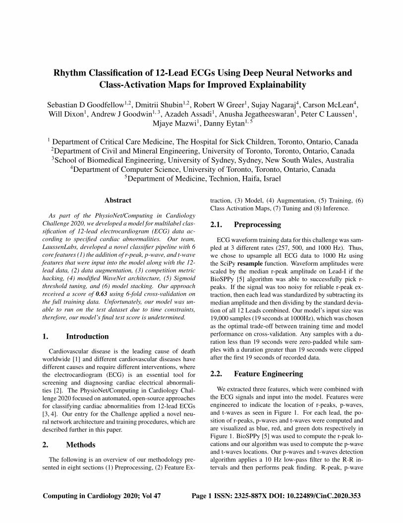
We extracted three features, which were combined withthe ECG signals and input into the model. Features wereengineered to indicate the location of r-peaks, p-waves,and t-waves as seen in Figure 1. For each lead, the po-sition of r-peaks, p-waves and t-waves were computed andare visualized as blue, red, and green dots respectively inFigure 1. BioSPPy [5] was used to compute the r-peak lo-cations and our algorithm was used to compute the p-waveand t-waves locations. Our p-waves and t-waves detectionalgorithm applies a 10 Hz low-pass filter to the R-R in-tervals and then performs peak finding. R-peak, p-wave
Figure 1. Example of ECG data and r-peak, p-wave andt-wave features.
and t-wave times were combined using a kernel densityapproach to generate a 1D normalized signal, which effec-tively provides their likelihood locations. These featureswere designed to help the model learn these important fea-tures thus, helping improve convergence.
2.3. Model
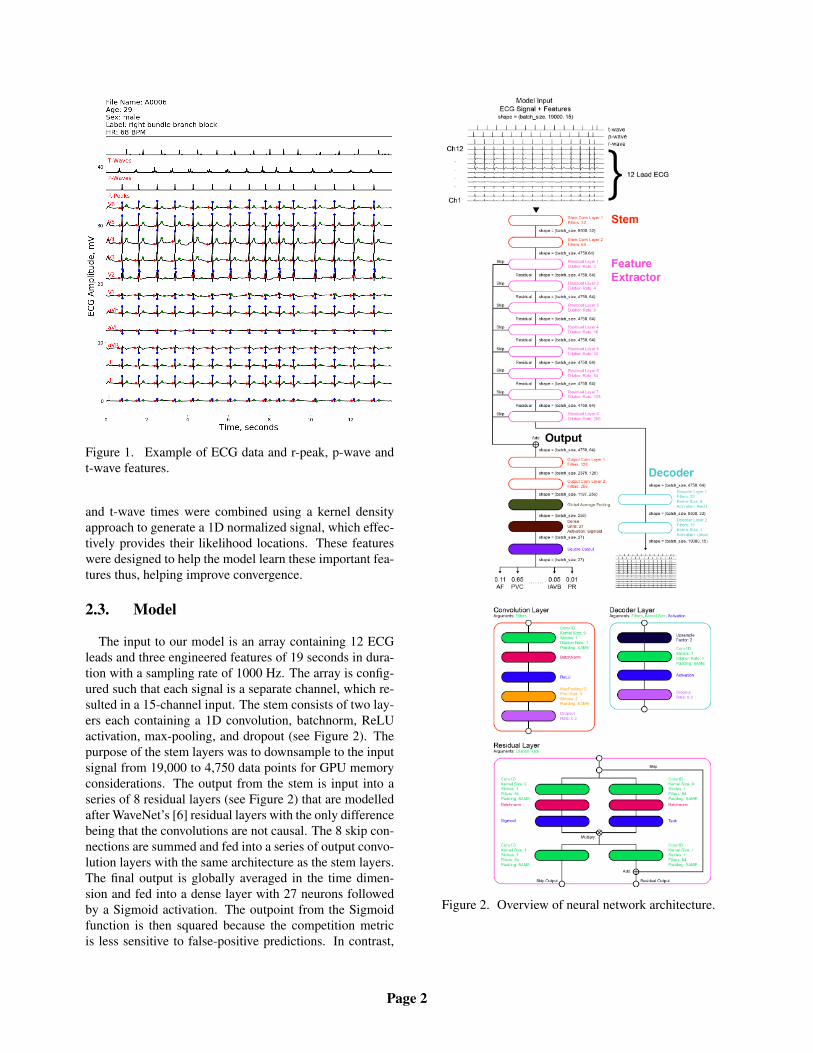
The input to our model is an array containing 12 ECGleads and three engineered features of 19 seconds in dura-tion with a sampling rate of 1000 Hz. The array is config-ured such that each signal is a separate channel, which re-sulted in a 15-channel input. The stem consists of two lay-ers each containing a 1D convolution, batchnorm, ReLUactivation, max-pooling, and dropout (see Figure 2). Thepurpose of the stem layers was to downsample to the inputsignal from 19,000 to 4,750 data points for GPU memoryconsiderations. The output from the stem is input into aseries of 8 residual layers (see Figure 2) that are modelledafter WaveNet’s [6] residual layers with the only differencebeing that the convolutions are not causal. The 8 skip con-nections are summed and fed into a series of output convo-lution layers with the same architecture as the stem layers.The final output is globally averaged in the time dimen-sion and fed into a dense layer with 27 neurons followedby a Sigmoid activation. The outpoint from the Sigmoidfunction is then squared because the competition metricis less sensitive to false-positive predictions. In contrast,
Figure 2. Overview of neural network architecture.
Page 2
it simulates the uplift prediction over recognizing all sig-nals as normal sinus rhythm. Since Sigmoid outputs aredistributed between 0 and 1, the squaring operation forcesthe model to give a higher penalty to false-negative predic-tions rather than false-positive predictions. In addition tothis output, a decoder was positioned after the last residuallayer where two decoder layers upsampled the data to itsoriginal input shape (batch-size, 19000, 15). The purposeof this auxiliary output was to improve the feature extrac-tion pipeline. Instead of learning features for classificationonly, it also tries to represent morphological features of theinput ECG signal.
2.4. Augmentation
During our exploratory data analysis, we notice manycommon noise artifacts in the data, such as baseline wan-dering, and our initial plan was to filter them out duringpre-processing. However, when experimenting with themodel, we observed superior performance when the datawas left unfiltered. Therefore, we decided to augment thedata with synthetic noise. We developed four syntheticnoise sources that we randomly added to the data dur-ing training (1) Gaussian noise, (2) high-frequency/low-amplitude oscillations, (3) baseline wandering, and (4)large-amplitude transient pulses. Two additional augmen-tation strategies were employed. The first applied a ran-dom multiplication factor to the waveform amplitude andthe second randomly perturbed the heart rate of the signal.For example, if the true heart rate was 124 BPM, we wouldadd a random fluctuation changing the value to 132 BPMand then resampling to 1000 Hz. This was only performedfor training samples where the label was not heart rate de-pendent.
2.5. Training
For training, the data was split into 6 folds forcross-validation using the open-source package iterative-stratification, which is designed for multilabel stratifica-tion. The model was trained for 100 epochs with earlystopping with and patience set to 10. The learning rate wasinitially set to 1e-3 (batch size 128) and followed a decayschedule ReduceLROnPlateau with patience equal to 1.The loss function was the sum of the binary cross-entropyof the classifier and mean squared error of the decoder andwas Optimized using the Adam optimizer [7].
2.6. Class Activation Maps
Our model architecture was designed such that ClassActivation Maps (CAMS) could be computed. We fol-lowed the 1D CAM formulation of Goodfellow et al.(2018) [8]. Goodfellow et al. (2018) [8] initially con-
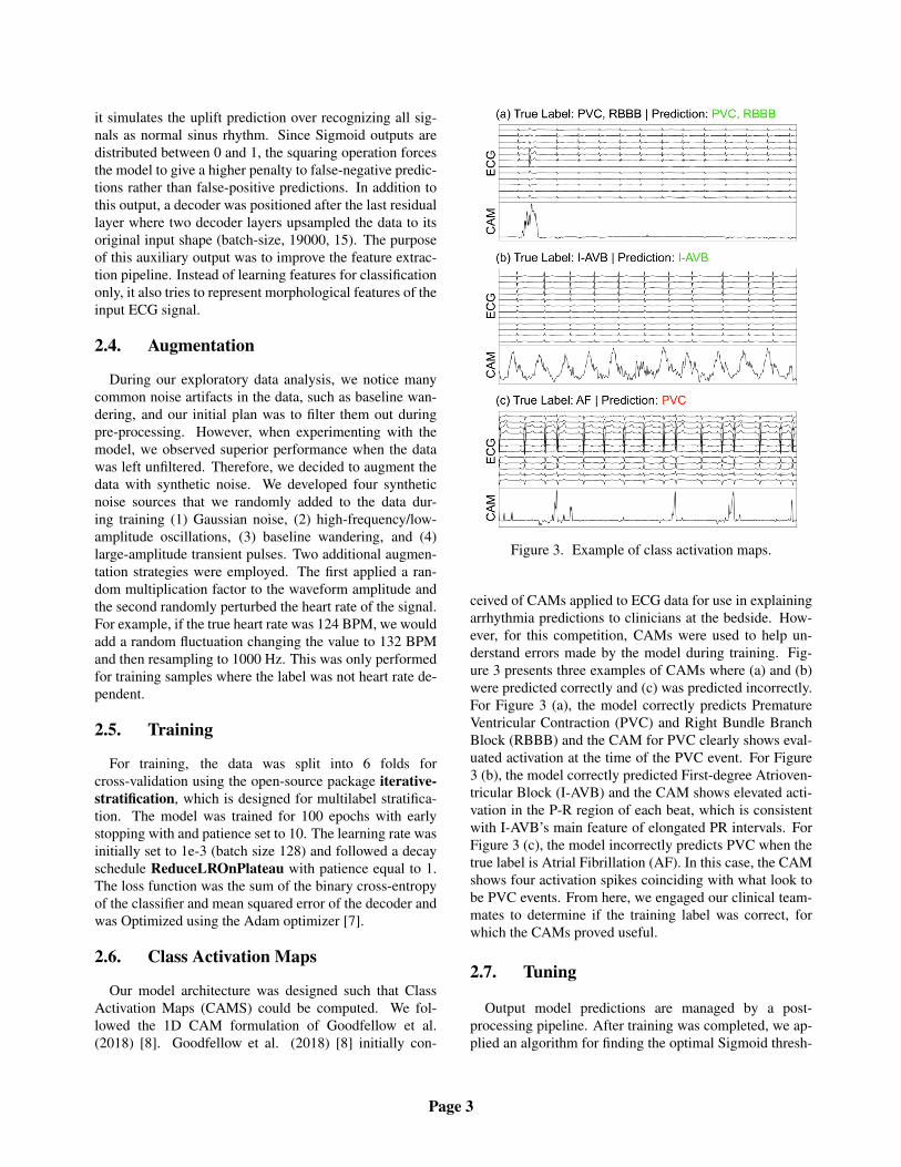
Figure 3. Example of class activation maps.
ceived of CAMs applied to ECG data for use in explainingarrhythmia predictions to clinicians at the bedside. How-ever, for this competition, CAMs were used to help un-derstand errors made by the model during training. Fig-ure 3 presents three examples of CAMs where (a) and (b)were predicted correctly and (c) was predicted incorrectly.For Figure 3 (a), the model correctly predicts PrematureVentricular Contraction (PVC) and Right Bundle BranchBlock (RBBB) and the CAM for PVC clearly shows eval-uated activation at the time of the PVC event. For Figure3 (b), the model correctly predicted First-degree Atrioven-tricular Block (I-AVB) and the CAM shows elevated acti-vation in the P-R region of each beat, which is consistentwith I-AVB’s main feature of elongated PR intervals. ForFigure 3 (c), the model incorrectly predicts PVC when thetrue label is Atrial Fibrillation (AF). In this case, the CAMshows four activation spikes coinciding with what look tobe PVC events. From here, we engaged our clinical team-mates to determine if the training label was correct, forwhich the CAMs proved useful.
2.7. Tuning
Output model predictions are managed by a post-processing pipeline. After training was completed, we ap-plied an algorithm for finding the optimal Sigmoid thresh-
Page 3
old by iterating over all thresholds between 0.05 and 0.95with a 0.05 step, calculating the competition metric and se-lect the best one. The optimal threshold was found for thetraining split and then applied to the validation set. Find-ing the threshold on the training set prevented leakage andmitigated the influence of incorrect labels.
2.8. Inference
At inference time, the six models trained for each cross-validation split were used for prediction. Hard predictionsfrom each model were combined by a majority vote. Thishelped improve generalization of the final predictions andmitigated the influence of incorrect labels. Consideringthat each model was trained on different incorrectly la-belled data, the resulting outputs are more independent andtherefore, provide a more robust group prediction.
3. Results
Our model’s cross-validation scores are presented in Ta-ble 1 and show a minimum of 0.614, a maximum of 0.644,and a mean of 0.63. Unfortunately, we were unable toget out model to run on the test dataset by the competi-tion deadline. As a result, we were given a test score of-0.406, which is the score if all predictions are 0 for all testsamples.
Table 1. Summary of model cross-validation and test per-formance.
Our CV score of 0.63 was the result of exhaustive modelarchitecture experimentation and hyper-parameter tuning.Unfortunately, the competition came to a close, however,our next strategy would have been relabelling. We devel-oped a Python application for our clinical teammates to al-low them to view ECG samples where the model made anincorrect prediction and provide feedback and label cor-rections. From inspecting many samples with our clini-cal teammates, it was clear that a large number of training
samples appeared to be miss-labelled. See Figure 3 (c)for a clear example. We also attempted to use gender andage features by concatenating them to the output from theglobal average pooling layer, however, this resulted in aminor decline in performance and was therefore not im-plemented.
In conclusion, we develop a novel model architectureand training strategy for the 2020 Physionet/CinC Chal-lenge which produced a CV score of 0.63. Unfortunately,we were unable to get a successful test score by the com-petition deadline. Our competition code is available atgithub.com/Seb-Good/physionet-challenge-2020.
References
[1] Benjamin EJ, Muntner P, Alonso A, Bittencourt MS, Call-away CW, Carson AP, Chamberlain AM, Chang AR, ChengS, Das SR, et al. Heart Disease and Stroke Statistics – 2019Update: a report From the American Heart Association. Cir-culation 2019;.
[2] Kligfield P. The centennial of the Einthoven electrocardio-gram. Journal of Electrocardiology 2002;35(4):123–129.
[3] Goldberger AL, Amaral LA, Glass L, Hausdorff JM, IvanovPC, Mark RG, Mietus JE, Moody GB, Peng CK, StanleyHE. PhysioBank, PhysioToolkit, and PhysioNet: Compo-nents of a new research resource for complex physiologicsignals. Circulation 2000;101(23):e215–e220.
[4] Perez Alday EA, Gu A, Shah A, Robichaux C, Wong AKI,Liu C, Liu F, Rad BA, Elola A, Seyedi S, Li Q, Sharma A,Clifford GD, Reyna MA. Classification of 12-lead ECGs: thePhysioNet/Computing in Cardiology Challenge 2020. UnderReview 2020;.
[5] Carreiras C, Alves AP, Lourenco A, Canento F, Silva H, FredA, et al. BioSPPy: Biosignal processing in Python, 2015.URL https://github.com/PIA-Group/BioSPPy/. [Online; accessed 2020].
[6] van den Oord A, Dieleman S, Zen H, Simonyan K, VinyalsO, Graves A, Kalchbrenner N, Senior A, Kavukcuoglu K.Wavenet: A generative model for raw audio. arXiv preprintarXiv160903499 2016;.
[7] Kingma DP, Ba J. Adam: A Method for Stochastic Opti-mization. In Proceedings of 3rd International Conference forLearning Representations, San Diego. 2015; .
[8] Goodfellow SD, Goodwin A, Greer R, Laussen PC, MazwiM, Eytan D. Towards understanding ECG rhythm classifica-tion using convolutional neural networks and attention map-pings. In Proceedings of Machine Learning for Healthcare2018 JMLR WC Track Volume 85, Aug 17–18, 2018, Stan-ford, California, USA. 2018; .
Address for correspondence:
Sebastian GoodfellowUniversity of Toronto, Toronto, Ontario, [email protected]