Eastern Illinois University e Keep Masters eses Student eses & Publications 1992 Ricardian Equivalence or the Indifference Between Tax and Debt Financing Chad Moutray is research is a product of the graduate program in Economics at Eastern Illinois University. Find out more about the program. is is brought to you for free and open access by the Student eses & Publications at e Keep. It has been accepted for inclusion in Masters eses by an authorized administrator of e Keep. For more information, please contact [email protected]. Recommended Citation Moutray, Chad, "Ricardian Equivalence or the Indifference Between Tax and Debt Financing" (1992). Masters eses. 2148. hps://thekeep.eiu.edu/theses/2148
Transcript
Eastern Illinois UniversityThe Keep
Masters Theses Student Theses & Publications
1992
Ricardian Equivalence or the Indifference BetweenTax and Debt FinancingChad MoutrayThis research is a product of the graduate program in Economics at Eastern Illinois University. Find out moreabout the program.
This is brought to you for free and open access by the Student Theses & Publications at The Keep. It has been accepted for inclusion in Masters Thesesby an authorized administrator of The Keep. For more information, please contact [email protected].
Recommended CitationMoutray, Chad, "Ricardian Equivalence or the Indifference Between Tax and Debt Financing" (1992). Masters Theses. 2148.https://thekeep.eiu.edu/theses/2148
TO: Graduate Degree Candidates who have written formal theses.
SUBJECT: Permission to reproduce theses.
The University Libra.ry is receiving a number of requests from other institution" asking permission to reproduce dissertations for inclusion in their library ho~dings. Altho"Ugh no copyright laws are involveq, we feel that professional courtesy demands that permission be obtained from the author before we ~llow theses to be copied.
Please sign one of the following statements:
Booth Library of Eastern Illinois University has my permission to lend my thesis t9 a. reputable college or university for the purpose of copying it for inclusioA in that institution• s library or research holdings.
7-7- f~ Date
I respec~ully request Booth Library of Eastern Illinois University not
allow my thesis be reproduced because ------------.....---
Date Author
m
Ricardian Equivalence or the Indifference
Between Tax and Debt Financing (TITLE)
BY
Chad Moutray
THESIS
SUBMITTED IN PARTIAL FULFILLMENT OF THE REQUIREMENTS
FOR THE DEGREE OF
Master of Arts in Economics
IN THE GRADUATE SCHOOL, EASTERN ILLINOIS UNIVERSITY
CHARLESTON, ILLINOIS
1992 YEAR
I HEREBY RECOMMEND THIS THESIS BE ACCEPTED AS FULFILLING
THIS PART OF THE GRADUATE DEGREE CITED ABOVE
Ml- 7~ l?!.2 (/ DAfE
Abstract
Ricardian equivalence is a topic which has attracted much attention in the
economic journals in the past couple of decades. Economic theory states that a tax cut
gives the public a greater disposable income. Thus, the public will consume more, and
the economy will grow. However, if the tax cut is fmanced by debt, the public will
perceive that a future tax increase is inevitable to pay off the debt. Under this scenario,
the public will not consume more. Instead, they will save all of their increased
disposable income in anticipation of thefuture tax increase. Ricardian equivalence then
is that the value of the tax cut is equal to the present value of the future tax increase.
This paper tests Ricardian equivalence within the context of the Patinkin
framework, using a single reduced-form equation. A regression analysis is performed
on the interest rate using real GNP, real tax receipts, additional real public debt, the
change in the price level, real government expenditures, and real money supply. This
study fmds that the data used for the time period 1975: 1 to 1991 :4 are consistent with
that of Ricardian equivalence.
Dedication
As I prepare to finally leave to pursue a Ph.D. in economics at Southern Illinois
University at Carbondale, I would like to dedicate this paper to my parents, Steven and
Patricia Moutray of Mattoon, Illinois. Without their love and support over the years,
I would never have made it this far.
Acknowledgements
I would like to thank my thesis advisor, Dr. Minh Dao, for all of his helpful
advice and instruction during the formulation of this thesis. In addition, I also
appreciate the beneficial comments of my other thesis committee members, Dr. Patrick
Lenihan and Dr. Paul Straub.
I want to also thank all of the economics department faculty, including our
secretary, Lois Luallen. They have been extremely helpful during my years here at
Eastern Illinois University. I have learned a lot from th~ both inside and outside the
classroom. In particular, I want to thank the chairman, Dr. EbrahimK.arbassioon. He
IX. References.................................................................................................. 34
1
Ricardian Equivalence or the Indifference Between Tax and Debt Financing
By Chad Moutray
I. Introduction
As the Federal government continues to finance its operations more and more
through debt, many economists have focused their attention on the effects of running
deficits on economic activity. This has led many to take a long-term approach to
analyzing what we are doing to future generations in this country. Many agree that by
continuing our policy of borrowing to maintain our current standard of living we are
mortgaging the futures of our children. But as this debate looms, another one stirs in
the background; some economists believe that attempts to stimulate the economy
through fiscal policy (such as the tax cuts that we experienced in the early 1980's) are
in vain. The concept of a Ricardian equivalence is one that numerous journal articles
have discussed in recent years. This paper will introduce the idea of Ricardian
equivalence and attempt to prove or disprove its existence in the context of the Patinkin
model.
It is important to first begin with the traditional view of how fiscal policy can
stimulate the economy before going into the more complex issue of Ricardian
equivalence. A measure of economic activity in a given country is the gross national
· product, or GNP. The GNP is the sum of personal consumption, private investment,
government expenditures, and net exports. Thus, it is easy to show that an increase in
government expenditures will increase GNP and, therefore, the nation's income. A tax
cut, on the other hand, can stimulate the economy by putting more money in the hands
of the consumer (a higher level of disposable income); thus, a tax cut can also raise
GNP.
The above textbook illustration of fiscal stimulus is widely accepted and taught
2
in principles of economics courses, but differences arise when that fiscal stimulus, a tax
cut perhaps, is financed by debt. This is where Ricardian equivalence becomes
important. The logic is simply that the taxpayer/consumer is smart enough to know
that a tax cut which is underwritten by borrowing today will have to be paid off at some
later date. Thus, fiscal stimulus today will have to be met with a fiscal contraction down
the road. Since the consumer will see the increase in his disposable income as only
temporary, or "transitory," he will not increase his consumption as expected under the
traditional view. Consequently, he will save his transitory income in expectation of the
future contraction, a tax increase perhaps. The Ricardian equivalence implies then that
the value of the tax cut equals the present value of the future tax increase. In addition,
Gertrud M. Fremling and John R. Lott, Jr. (1989) argue that Ricardian behavior
prompts the consumer not only to save up for the expected future tax increases but also
to compensate for future deadweight loss increases which are caused by the tax
mcreases.
This paper will first introduce a survey of current literature on Ricardian
equivalence in section II. From there, section III will initially introduce the Patinkin
model and then set up a model that will be tested in this paper. Empirical results will
appear in section IV. Once the fmdings have been stated, their implications will be
discussed in section V, and then suggestions for further research will end the paper with
section VI.
3
II. A Survey of the Literature
Robert J. Barro, an economics professor at Harvard, fueled the current
discussion on Ricardian equivalence. In the November/December 1974 issue of the
Joumal of Political Economy, Barro surfaced the concept in his article, "Aie
Government Bonds Net Wealth?" He states that consumers behave as if "they were
infinitely lived," and thus, as long as "an operative chain of intergenerational transfers
which connected current to future generations" exists, then government bonds would
produce neutral effects (p. 1116). He then goes on to say:
"The basic conclusion is that there is no persuasive theoretical case for treating government debt, at the margin, as a net component of perceived household wealth. The argument for a negative wealth effect seems, a
priori, to be as convincing as the argument for a positive effect. Hence, the common assertion (as in Patink.in 1962, chap. 12, p. 289) that the marginal net-wealth effect of government bonds is somewhere between zero and one and is most likely to lie at some positive intermediate value that has no a priori foundation. If, in fact, the marginal net-wealth effect were negligible, the implications for monetary and fiscal analysis would be far-reaching" (p. 1116).
Since then, a number of prominent economists have entered the arena to either support
or denounce the Ricardian equivalence.
Paul Evans agrees wit~ Barro that government debt is neutral. He formulates
a linear equation for the expected steady-state interest rate. Then by fmding the values
of the parameters, debt neutrality can be tested. Evans writes in his 1989 article,
"A linear version of the model under consideration is:
where r·t, d•t' and g•t are, respectively, the expected steady-state real interest rate, and the expected steady-state ratios of the government debt and government spending to output; the expectations are those of bond
4
traders during period t; f3 d and P 8 are parameters; and ut is an error term . . . . If government debt is neutral, then Pd=O and P8=0; if government wealth is net wealth, then Pd>O and P8>0" (1989, p. 41).
His paper concludes that Pd<O (increasing the Federal debt lowers the interest rate);
therefore, government-debt neutrality is then assumed since the value of the parameter
is negative.
According to :8. Douglas Bernheim., a critic of Ricardian equivalence, there are
seven assumptions that must be made in order for it to be valid. He writes:
"These include: 1) successive generations are linked by altruistically motivated transfers; 2) capital markets are either perfect, or fail in specific ways; 3) consumers are rational and farsighted; 4) the postponement of taxes does not redistribute resources across families with systematically different marginal propensities to consume; 5) taxes are non-distortionary; 6) the use of deficits cannot create value (not even through bubbles); and 7) the availability of deficit financing as a fiscal instrument does not alter the political process" (1989, p. 63).
Of these assumptions, it would be easy to find fault with some of them. Like the ideal
situations of perfect competition, though, Ricardian equivalence is only expected to
approximate reality. Thus, the suggestion that consumers are "rational and farsighted"
is not necessarily a fatal flaw.
What Bernheim feels is the most troubling about the Ricardian equivalence
theorem is the concept of altruistically-motivated intergenerational transfers, or
bequests. For an explanation of why these become relevant. it is necessary to quote
Robert J. Barro:
"Consider a deficit-fmanced tax cut, and assume that the higher future taxes occur partly during the typical person's lifetime and partly thereafter. Then the present value of the first portion must fall short of the initial tax cut, since a full balance results only if the second portion is included. Hence the net wealth of persons alive rises, and household react by increasing consumption demand. Thus. as in the standard approach sketched above, desired private saving does not rise by enough
5
to offset fully the decline in government saving" (1989, p. 40).
Barro then goes on to suggest that the results depend on whether or not "the typical
person feels better off when the government shifts a tax burden to his or her
descendants" or "is already giving to his or her children out of altruism" (p. 40). In
arguing in support of bequests as a method for maintaining Ricardian equivalence,
Barro notes that these transfers do not have to be upon death only; they can also be in
the form of gifts given during the lifetime or even paying for their child's education (p.
41). But Martin Feldstein disagrees with the notion that "such in-kind transfers" have
similar effects as bequests since they involve additional spending. Thus, "a taX
reduction can increase current consumer spending [via these in-kind transfers]" (1982,
p. 5), a clear violation of Ricardian equivalence.
For his part, Bernheim disagrees with the assumptions made by Barro. First of
all, he states that, "Due to the linkages between families, it is in general impossible to
represent any particular family (or set of families) as a single, utility-maximizing agent,
even when the well-being of each individual is assumed to depend only on his own
consumption and well-being of his children" (1989, p. 64). The next problem with this
line of reasoning is that transfers mainly occur among the very rich; although, some do
occur in other socioeconomic classes. In fact, Bernheim writes, "Finally, several authors
(e.g. Diamond and Hausman, 1984) have found that roughly 20 percent of the
population arrives at retirement with essentially no bequeathable assets. Other evidence
indicates that the receipt of gifts from children is relatively uncommon (Hurd, 1987b )"
(p. 66-7). In addition, it is also possible for a transfer to be negative, according to
Martin Feldstein; "A parent who believes that, because of generally rising productivity
and real incomes, his children will be richer than him.self, may well decide that the
optimal 'bequest' is negative, i.e., a transfer from his children to himseJr' ( 1982, p. 5).
Bernheim's third reason is that some bequests are accidental (due to an untimely death)
6
and others might have "alternative motivations;" these could interfere with Barro's
assumptions and alter the results (p. 67). Finally, Bernheim. argues that not all bequests
are born out of altruism; instead, a strategic bequest motive is used so that the parent
can influence the child's behavior. Thus, a "credible threat" by the parent can result in
leaving a larger transfer to a well-behaved child.
Other author~ have also dealt with the intergenerational transfer area. James
Andreoni developed an impure altruism model in which individuals receive a "warm
glow" from giving to others. His model treats consumption as a public good. For
parents giving to their children, he says that "Parents are taken as altruistic: they care
about their own consumption, xP, and the consumption of th~ir heir, xh. Since the heir
also cares about Xii, it is a public good" (1989, p. 1456). He then proceeds to develop the
utility functions of the two, which are:
UP = UP (xP, xh, b) where b = bequests uh= uh (xJ
In maximizing each one's utility, it is important to note that:
"Parents are impurely altruistic with respect to their gifts to heirs, while the heirs can be thought of as 'purely altruistic' with their own consumption. As such, redistributions from children (more altruistic) to parents (less altruistic) will reduce the private supply of the public good (the consumption of the heir). Parents will be unwilling to perfectly substitute bequests for debt; hence they will keep some of their new 'wealth' for themselves" (p. 1456).
A similar result will occur if instead of the parents leaving a bequeath to the child. the
child is giving (gifts) to the parent; thereby, the consumption of the parent is the public
good. It, too, creates a result which is non-neutral and conflicts with Ricardian
equivalence. In a paper by Laurence J. Kotlikoff, Assaf Razin, and Robert W.
Rosenthal, they explore this possibility that both the parent and the child are altruistic.
"Barro does not make explicit the game he models between an altruistic
7
parent and child, but in his formulation the child appear to be quite passive and simply takes whatever transfer is given. There is no scope for the child to manipulate the parent by threatening to refuse transfers that are below a specified level and/or by threatening to the parent if the parent is not sufficiently generous" (p. 1261).
By maximizing the utility functions of both the parent and the child, these authors reach
a similar conclusion that government policy is non-neutral and does increase
consumption.
Turning away from altruistic transfers, another area of disagreement is that the
uncertainty over future income and taxes can lead to problems with Ricardian
equivalence. Martin Feldstein, for instance, has argued that when there is uncertainty,
Ricardian equivalence fails (1988, p. 22). However, William A. Bomberger responded
to Feldstein by saying that introducing uncertainty into the model only complicates the
process "unnecessarily" and that uncertainty does not really cause the theory to fail
(1990, p. 312). Furthermore, it should be mentioned that when progressive taxes are
introduced into the model instead of lump sum, many economists (for example, Kimball
and Mank.iw 1989) have found that the overall result is somewhat altered. For his
part, Barro argues that taxes are "smoothed out" over time and has found in his studies
that the budget deficits between 1916 and 1983 can be explained in this way. To
illustrate, he writes:
"For example, if time periods are identical except for the quantity of government purchases - which are assumed not to interact directly with labor supply decisions -- optimality dictates uniform taxation of labor income over time. This constancy of tax rates requires budget deficits when government spending is unusually high. such as in wartime, and -surpluses when spending is unusually low" (1989, p. 46).
Thus. due to this smoothing-out effect. Barro suggests that the uncertainty over taxes
and the timing of taxes will not affect the economy in a way that would unravel the
8
Ricardian equivalence theorem due to the fact that tax rates are constant over time.
Miles S. Kimball and N. Gregory Mankiw, however, argue that while consumption
would have little impact in the short-run from a "tax rescheduling," long-term
repayment can significantly alter consumption, disproving Ricardian equivalence (1989,
p. 871-3).
The recent wave of journal articles has produced a number of empirical articles
on the subject of various effects of Ricardian equivalence on consumption.
Nonetheless, they have been rather inconclusive. For instance, Paul Evans ran
"instrumental variable regressions of consumption on lagged consumption and lagged
assets" over several sample periods. He found that tax cuts, including the Reagan tax
cut, did not appear to increase the level of consumption and upheld Ricardian
equivalence (1988). Similarly, James S. Fackler and W. Douglas McMillin looked at
the effects of government debt on the economy from 1963:2 through 1984:4. Using a
VAR methodology, they were able to improve the "robustness" of their results and
found that "the sum of domestically-held and foreign-held debt had non-trivial effects
on the long-term interest rate and output" (1989, p. 1002). But, the "impulse response
functions" show that the initial reaction is actually lm£g interest rates, output, and
prices. This could be explained by Roger C. Kormendi as individuals saving "more than
the present value of income streams" due to uncertainty over future taxes. This is not
consistent with the traditional thinking, and thus suggests that Ricardian equivalence
might be at work. Nevertheless, Bernheim argues that the differences in the many
articles can be traced to varying the null hypothesis and that there is a definite pro
Ricardian bias in the studies. He also states the need to look at permanent deficits,
instead of transitory. "Both Bernheim and [Bradford G.] Reid found that permanent
deficits significantly raise consumption as a fraction of national income. These results
are consistent with the Neoclassical paradigm" (1989, p. 69).
9
In a study by David Wilcox, the effects of unexpected policy changes on
consumption behavior are analyzed using the life~ycle hypothesis. According to the
theory, all known policy changes have already been included in an individual's level of
consumption. Unexpected modifications in policies will not alter consumption unless
the change is interpreted to be permanent; transitory changes will not have an effect on
consumption (1989, p. 289). In the article he uses Social Security benefit increases,
which are assumed to be expected because they are revealed in advance, and the timing
of their announcement to analyze their effects on consumption patterns. His
conclusions are that these raises result in large consumption increases, especially for
durable goods. This is true for a large number of observations and is "shown to be a
regular feature of the post-1965 data" (p. 303). This also helps to cast a shadow of
doubt on Ricardian equivalence because the Social Security increases tended to raise
aggregate demand.
Time-series regressions have also been used to test Ricardian equivalence.
Nicholas Sarantis tested data for Belgium, Finland, France, West Germany, Greece,
Italy, the Netherlands, Sweden, and the United Kingdom for 1960 to 1980. He tested
them one by one and as a group and found that fiscal variables had an impact on
consumer spending; the results were even stronger when the nine countries were tested
together. Sarantis therefore concludes that his findings are "consistent with the more
general view that changes in government expenditure, transfers, and taxes can exert
substantial effects on aggregate demand" (1985, p. 245). Holcombe, Jackson, and
Zardhoohi tested the impact of government debt on per capita personal savings for the
United States from 1929 to 1976. Their findings were that for every dollar of additional
debt, 20 cents of it would be saved~ the other 80 cents would be passed on as a future
burden ( 1981 ).
10
ID. The Model
Having introduced the literature that is relevant to this paper, it is now time to
develop a model testing the Ricardian equivalence thereom. While reading the many
articles on this subject, I was still daunted by the fact that during the 1980's debt
accumulated at record proportions. Even Barro, who advanced the tax-smoothing
concept mentioned before, added the disclaimer, "although the deficits since 1984 tum
out to be substantially higher than predicted" (1989, p. 47). We have watched as
government debt at all levels, corporate and business debt, and individual debt have
skyrocketed over the past few decades. Indeed, many economists blame the current
sluggishness of the economy on the fact that we are now paying off some of our debt
(with the notable exception of government). Indeed, Paul Evans found that the Reagan
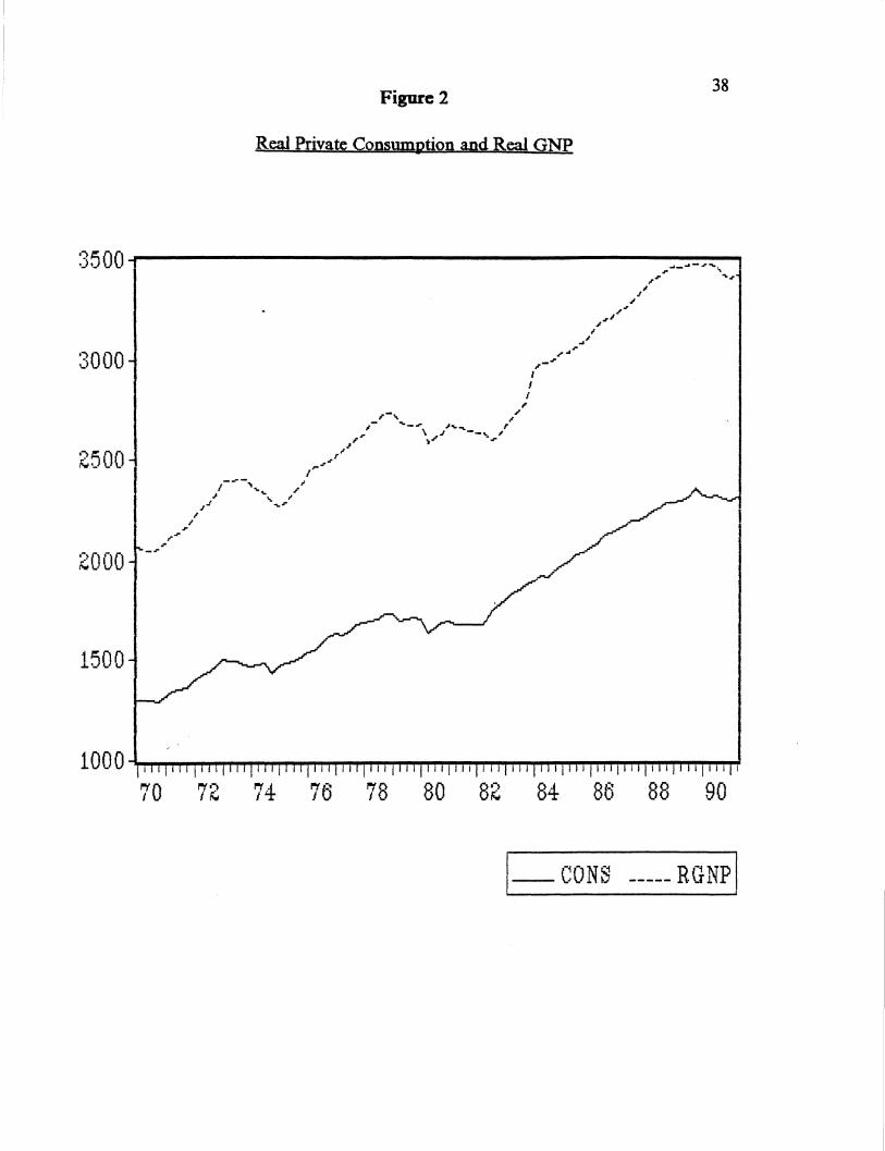
tax cuts did not affect consumption. But to the naked eye, something did happen to
consumption in the 1980's. Figure 1 shows private consumption adjusted for inflation
using 1980 as the base year and the Federal government deficit for each quarter 1970: 1
through 1991:2. Notice that consumption departs from its trend around 1983;
meanwhile, the deficit continues to become larger. Figure 3 shows the "marginal tax
burden" (or the Federal tax plus the FICA tax rate) for these same years; notice that the
tax burden begins to fall drastically around 1982-83. Was it just a coincidence that the
growth in real consumption steadily increased as tax rates fell? Notice also that Figure
4 shows the yield on long-term U.S. Bonds; the yields have also dropped since their peak
in 1981-82. The examination of these statistics might lead to the premature assumption
that Ricardian equivalence has not held up during the last twenty plus years, but these
statistics alone do not prove anything. So the next step is to come up with a
macroeconomic model which can be used to test Ricardian equivalence.
To begin with, I will introduce the work of T. Windsor Fields and William R.
11
Hart. Their 1990 article in Economic Inquiry was essentially a "teaching tool" so that
professors would be able to teach Ricardian equivalence to undergraduates using the
IS-LM framework. They began with the basic IS and LM equations, but disposable
income is redefined to reflect the reality that consumers would view an increase in bond
financed government expenditures as a future increase in taxes. Therefore, they use the
following equation:
(1) Y = C(Y-G) + I(R) + G
This is the standard identity that GNP equals consumption plus investment plus
government expenditures. In this equation, national income, or gross national product,
is denoted as a Y. Government expenditures are G, and the interest rate is an R.
Consumption is defmed as a C and is a function of disposable income (using
government expenditures instead of taxes), and investment is a function of the interest
rate. Now, since taxes are no longer a consideration in the model, a tax cut fmanced by
bonds will have no effect on consumption. Their LM equation does not need to change
for Ricardian equivalence to hold, according to the two authors.
Before proceding further, it is important to introduce the Patinkin model. This
model has four assumptions. First, there is full employment in the labor market; thus,
labor supply equals labor demand. Second, there is no money illusion; consumers and
workers are aware of the effects of inflation on prices and wages. Next, the marginal
propensity to consume does not change with income. Finally, no one expects any
inflation in the future.
Under this scenario, there are four markets. The first, which was mentioned
earlier, is µie labor market. Equilibrium in the labor market, written in the form of
labor demand equals labor supply, would appear as follows:
(2) Y(W/P, KJ = R(W/P)
The real wage is denoted as nominal wage, or W, over the price level, or P, and Ko
12
denotes the capital stock. The real wage has a negative effect on labor demand and a
positive one on labor supply. The more capital that is used in the process, the more
productive labor; thus, it has a positive impact on labor demand. The first assumption
of the Patinkin model is full employment, and this equation satisfies it. The next market
is the commodity market; in equilibrium, it is written as:
(3) F(Y0, R, MJP) = S(W/P, KJ = Y0
Y0 is the commodity supply (it is equal to S(W/P, KJ because of the full employment
assumption). The nominal money supply is denoted with an M0; the interest rate is R.
Fis the commodity demand function, and Sis the commodity supply function. Income
and the real money supply have a positive effect on the commodity demand; whereas,
higher interest rates lower commodity demand. The bond market is the third. In
equilibrium, it appears as follows:
(4)
Nominal money balances held by households are denoted as Mo HH' and MoF indicates
money held by firms. The price of a bond is l!R. Income has a positive impact on both
bond demand and supply; the price of the bond positively influences bond supply but
negatively affects oond demand. The more money held by households, the greater the
bond demand; but, the more money held by firms, the lower the bond supply. The final
market is the money market, which in equilibrium is written as follows:
( 5) MJP = L(Y 0, R, MJP)
Income and real money balances have a positive effect on the demand for real money
balances; while, the interest rate negatively impacts it.
Having introduced the four markets, it is important to state that the labor
market can be left out for our purposes because of the full employment assumption,
assumes flexible prices and nominal wages, i.e., real wages will always adjust to ensure
full employment. Moreover, because ofWalras' Law (which asserts that if two markets
13
are in equilibrium, then the third one is as well), only the commodity and money
markets will be used for analysis. The two markets in equilibrium can be represented
by a CC and an LL curve. The CC curve represents combinations of Rand P such that
the commodity market is in equilibrium. On the other hand, the LL curve shows
combinations of Rand P such that the money market is in equilibrium. Where these
two curves cross (CC has a negative slope and BB a positive slope) is considered a
general equilibrium for the four markets (the labor market is always in equilibrium and
the bond market is because ofWalras' Law).
When .incorporating the government sector, the standard Patinkin model takes
the following form for the CC and the LL curves:
(6) Y = F(Y-T, R, MJP +kV/RP)+ G (7) MJP = L(Y-T, R, Mp+ kV/RP)
In these equations, Y is defined as income (or output), and, therefore, since T denotes
taxes, Y-T is disposable income. The interest rate is R; government spending is G. The
wealth effect is subdivided into two parts. The first, MJP, is the real value of money
holdings, and the second, kV /RP, is the real value of bond holdings. The k value is
what was described earlier in the paper in a quotation by Barro as the marginal net
wealth effect. If k=O, Ricardian equivalence will hold because everyone is concerned
about future taxes; if k=l, no one is concerned about future taxes. If the disposable
income component is changed to Y-G, as Fields and Hart have used when integrating
Ricardian equivalence in the context of the IS-LM model, then the new CC and LL
curves would appear as:
(8) Y = (Y-G, R, MJP +kV/RP)+ G (9) MJP = (Y-G, R, MJP +kV/RP)
Trying to differentiate and solve these equations to fmd the change in output with
respect to a change in fiscal policy is quite horrendous, especially since the fmal result
14
is inconclusive due to the fact that the value of k is unknown. Ifk=O, though, then the
change in output would exactly equal the change in government expenditures ( dy=dg).
But if k>O, then the output change will more than likely outstrip the change in
government expenditures ( dy>dg) and Ricardian equivalence will not hold.
The next step is to specify an aggregate supply function. In this model the
commodity supply is a function of the price difference in two consecutive time periods.
The total commodity demand, like the Patinkin model, consists of a private component
which is a function of disposable income, the interest rate, the wealth effect (real money
balances), and a public component, namely, government expenditures. In this case the
private commodity function is assumed to be loglinear. The two equations then appear
as follows:
(10) Y = C0 + C1 (Pt - Pi,.1)
(11) y1 =Ao + A1 log(Y" - T) + Ai log R + A:i log(M/P) + G
Before going on, it is necessary to state that y• and yd denote commodity supply and
demand respectively, Pt is the current price, Pt.tis last year's price, Tis tax revenues, R
is the interest rate, and G is government spending. Ao through ~ are coefficients. If
commodity supply equals commodity demand, then the equilibrium condition is:
Solving for the log of disposable income, one obtains:
(13) log(Y' - n =(Co - AJIA1 + (C/A1) (P - Pl) - (AJA1) log r - CA:i/Al) log(M/P) --(l/A1) G
It is necessary now to derive the condition for money market equilibrium. In this
model the money supply is exogenous, and money demand is a function of disposable
income, the interest rate, and the wealth effect. Then the equations for money supply
Simply put, by taking each variable and subtracting from it the first lag times p and the
second lag times p 2, then second-order autocorrelation can be corrected (Newbold, p.
590).
L
References
Andreoni, James. "Giving with Im.pure Altruism: Applications to Charity and Ricardian Equivalence." Journal of Political Economy. December 1989; 1447-58.
34
Barro, Robert J. "Are Government Bonds Net Wealth?" Journal of Political Economy. November/December 1974; 1095-117.
Barro, Robert J. "The Ricardian Approach to Budget Deficits." Journal of Economic Perspectives. Spring 1989; 37-54.
Bernheim, B. Douglas. "A Neoclassical Perspective on Budget Deficits." Journal of. Economic Perspectives. Spring 1989; 55-72.
Bernheim, B. Dou~as and Kyle Bagwell. "Is Everything Neutral?" Journal of Political Economy. April 1988; 308-38.
Bomberger, William A. "The Effects of Fiscal Policy When Incomes Are Uncertain: A Contradiction to Ricardian Equivalence: Comment." American Economic Review. March 1990; 309-12.
Diamond, Peter A. and Jerry Hausman. "Individual Retirement and Savings Behavior." Journal of Public Economics. 1984, Volume 23; 81-114.
Evans, Paul. "Are Consumers Ricardian? Evidence for the United States." Journal of Political Economy. October 1988; 983-1004.
Evans, Paul. "A Test of Steady-State Government-Debt Neutrality." Economic lnQuiry. January 1989; 39-55.
Fackler, James S. and W. Douglas McMillin. "Federal Debt and Macroeconomic Activity." Southern Economic Journal. April 1989; 994-1003.
Feldstein, Martin. "The Effects of Fiscal Policy When Incomes Are Uncertain: A Contradiction to Ricardian Equivalence." American Economic Review. March 1988; 14-23.
L
Feldstein, Martin. "Government Deficits and Aggregate Demand." Journal of Monetary Economics. January 1982; 1-20.
35
Fields, T. Windsor and William R. Hart. "On Integrating the Ricardian Equivalence Thereom and the IS-LM Framework." Economic Inqpicy. January 1990; 185-93.
Fremling, Gertrud M .. and John R. Lott, Jr. "Deadweight Losses and the Saving Response to a Deficit." Economic Inguiry. January 1989; 117-29.
Henderson, J. Vernon, and William Poole. Principles of Economics. First Edition. Lexington, Massachusetts: D.C. Heath and Company, 1991.
Holcombe, Randall G., John D. Jackson, and Asghar Zardkoobi. "The National Debt Controversy." Kyk.los. 1981, Fasc. 2; 186-202.
Hurd, Michael D. "Mortality Risk and Bequests." Mimeo, SUNY, Stony Brook; 1987[b].
Kimball, Miles S. and N. Gregory Mankiw. "Precautionary Savings and the Timing of Taxes." Journal of Political Economy. August 1989; 863-79.
Kormendi, Roger C. "Government Debt, Government Spending, and Private Sector Behavior." American Economic Review. December 1983; 994-1000.
Kotlikoff, Laurence J., AssafRazin, and Robert W. Rosenthal. "A Strategic Altruism. Model in Which Ricardian Equivalence Does Not Hold." The Economic Journal. December 1990; 1261-8.
Newbold, Paul. Statistics for Business and Economics. Second Edition. Englewood Cliffs, New Jersey: Prentice Hall, 1988.
Patinkin, D. Money. Interest. and Prices. Second Edition. New Y or.le Harper & Row, 1964.
Reid, Bradford G. "Aggregate Consumption and Deficit Financing: An Attempt to Separate Permanent from Transitory Effects." Economic Inquity. 1985, Volume 23; 475-87.
Sarantis, Nicholas. "Fiscal Policies and Consumer Behavior in Western Europe." Kyklos. 1985, Fasc. 2; 233-48.
Simpson, Thomas D. ''The Redefined Monetary Aggregates." federal Reserve Bulletin. February 1980; 97-114.
36
Wilcox, David W. "Social Security Benefits, Consumption Expenditure, and the Life-Cycle Hypothesis." Journal of Political Economy. April 1989; 288-304.
Figure 1 37
Real Private Consumption and the Federal Budget Deficit
2500-------------------------250
2250
2000
1750
1500
70 72 74 76
' I \ I I
.,., I I I \ I I I I I \ I
\ I , I l,..i \ I ,,.
I I I I ' I ', I
'\ I' ..,,
80
~ I\ f\
~ ~/if\ /i \-"'\. I I I \ ~ \ I I I \ I I /~ I ',. /\)'\ 11 1 J ,1,1 ,,. /1 ?1 I ~ I I ~ I : ~ ii I I 11 t ' I 1 1,11 I I" : ... ~ 1ljl1 I I I \ I I I 11 I I I I/\ II i ~It I ,1 l I I I It I I 1 I I '4 I 11 \ J l I l \I I