NBER WORKING PAPER SERIES MACROECONOMIC PLANNING AND DISEQUILIBRIUM ESTIMATES FOR POLAND, 1955-1980 Richard Fortes Richard Quandt David Winter Stephen Yeo Working Paper No. 1182 NATIONAL BUREAU OF ECONOMIC HESEARCH 1050 Massachusetts Avenue Cambridge, MA 02138 August 1983 The research reported here is part of the NEER's research program in International Studies. Any opinions expressed are those of the authors and not those of the National Bureau of Economic Research.
Transcript
NBER WORKING PAPER SERIES
MACROECONOMIC PLANNING AND DISEQUILIBRIUMESTIMATES FOR POLAND, 1955-1980
Richard Fortes
Richard Quandt
David Winter
Stephen Yeo
Working Paper No. 1182
NATIONAL BUREAU OF ECONOMIC HESEARCH1050 Massachusetts Avenue
Cambridge, MA 02138
August 1983
The research reported here is part of the NEER's research programin International Studies. Any opinions expressed are those of theauthors and not those of the National Bureau of Economic Research.
NTBER Working Paper #1182August 1983
Macroeconomic Planning and Disequilibrium:Estimates for Poland, 1955—1980
ABSTRACT
This paper specifies and estimates a four—equation disequilibrium
model of the consumption goods market in a centrally planned economy
(CPE). The data are from Poland for the period 1955—1980, but the
analysis is more general and will be applied to other CPEs as soon as
the appropriate data sets are complete. This work is based on
previous papers of Portes and Winter (P—W) and Charemza and Quandt
(C—Q). P—W applied to each of four CPEs a discrete—switching
disequilibrium model with a household demand equation for consumption
goods, a planners' supply equation, and a "mm" condition stating that
the observed quantity transacted is the lesser of the quantities
demanded and supplied. C-Q considered how an equation for the
adjustment of planned quantities could be integrated into a CPE model
with fixed prices and without the usual price adjustment equation.
They made plan formation endogenous and permitted the resulting plan
variables to enter the equations determining demand and supply.
This paper implements the C—Q proposal in the P—W context. It uses
a unique new data set of time series for plans for the major
macroeconomic variables in Poland and other CPEs. The overall
framework is applicable to any large organization which plans economic
variables.
Richard Portes Richard QuandtDept. of Economics Dept. of Economics, Princeton University
Birkbeck CollegeLondon University David Winter
7/15 Gresse Street Dept. of Economics, Bristol University
LONDON W1P 1PAStephen Yeo
Tel: (01) 580 6622 x 412 Dept. of Economics, Birkbeck College
1 FLDABK
Macroeconomic Planning and Disequilibrium:Estimates for Poland, 1955—1980
Richard Portes, Richard Quandt, David Winter and Stephen Yeo
April 1983
1. Introduction
This paper specifies and estimates a four—equation disequilibrium
model of the consumption goods market in a centrally planned economy
(CPE). The data are from Poland for the period 1955—1980, but the
analysis is more general and will be applied to other CPE5 as soon as
the appropriate data sets are complete.
The work reported here is based on the previous papers of Portes
and Winter (1980) and Charemza and Quandt (1982), referred to below as
P—W and C—Q. The former applied to each of four CPE5 a
discrete—switching disequilibrium model with a household demand
equation for consumption goods, a planners' supply equation, and a
"mm" condition stating that the observed quantity transacted is the
lesser of the quantities demanded and supplied. C—Q considered how
t Portes is at Birkbeck College, University of London, and Ecole des
Hautes Etudes en Sciences Sociales, Paris, and is Research Associate,
National Bureau of Economic Research; Quandt is at PrincetonUniversity; Winter is at the University of Bristol; and Yeo is at
Birkbeck College. Quandt gratefully acknowledges support from the
National Science Foundation under grant SES—8012592. Portes and Yeo
thank the Social Science Research Council (U.K.) for support under
grant B00230048. Fortes has also benefitted from the assistance of
the Maison des Sciences de l'Homme. We are especially indebted to
T. Bauer, W. Charemza and M. Gronicki for assistance with time series
for plan variables, and to I. Grosfeld for help with Polish data.
I. Brunskill and A. Milne provided research assistance. We have
received incisive and helpful comments from Hugh Davies and Guy
Laroque.
The research reported here is part of the NBER's research program in
International Studies. Any opinions expressed are those of the
authors and not those of the National Bureau of Economic Research.
2 FLDABK
an equation for the adjustment of planned quantities could be
integrated into a CPE model with fixed prices and without the usual
price adjustment equation. They made plan formation endogenous and
permitted the resulting plan variables to enter the equations
determining demand and supply. Depending on the precise
specification of the equation determining the plan, the model could
adjust towards market clearing in a manner similar to that of
disequilibrium models with price adjustment equations.
This paper implements the C—Q proposal in the P—W context. It
differs from P—W in several respects: (1) the data are extended
beyond 1975, up to 1980; (ii) the main series have been more or less
substantially revised, using new information; (iii) a plan—adjustment
equation determines the published plan for aggregate consumption by
households; (iv) this plan enters the equation for the supply of
consumption goods; (v) the variables constructed by P—W to measure
deviations from plans for exogenous variables (output, investment,
defence expenditure), which proxied the plan series by second—order
quadratic trends, now use published plan data. The model here
differs from C—Q in having a more general form of plan—adjustment
equation than they propose.
The work reported here was possible only because we were able to
assemble reliable time series for plans for the major macroeconomic
variables in Poland and other CPEs. Using this new and unique data
set, our empirical work can now go beyond the question posed by P—W,
which concerned the existence of excess demand in the aggregate
consumption goods markets of CPEs, to a range of important questions
concerning the planning process and macroeconomic disequilibrium: Are
the plans in a CPE properly represented as endogenous, determined by
3 FLDABK
stable economic relationships rather than political caprice? How
do plans so determined then influence the planners and the economy?
Do the planners plan for macroeconomic equilibrium (i.e., does the
plan refer to their planned supply or to their intention for the
quantity transacted)? Is the disequilibrium macro framework
appropriate and useful for the analysis of CPEs (see Portes, 1981a)?
There are also interesting theoretical and econometric questions which
arise, some of which will provide material for future work. The
overall framework is applicable to any large organisation which plans
economic variables.
2. The Simple Disequilibrium Model
The basic framework of our general model for Poland is taken from
P—W with the modifications indicated above. Thus the consumption
demand equation is identical to that in P—W, derived directly from the
Houthakker—Taylor savings function:
CDt = cLiDNFA_i + c2DYD + cz3YD + u1(1)
where
CD = household desired expenditure on consumption goods andservices
DNFA = household saving, measured as the change in net financial
assets of households, NFA, during the period (NFA. is theend—of—period net stock of financial assets); DNFAt_i wascalled Si in P—W
DYD = change in disposable income from the previous to the
current period
YD = disposable income
u1 N(O, n )
Although it has a rather sophisticated theoretical rationale, this
4 FLDABK
essentially just makes consumption depend on current and lagged income
and on lagged consumption.t
The work of Houthakker and Taylor suggests the following a priori
hypotheses:
—l < a1 — 1/3, 0 < < 1, a = 1
The modified supply equation is
CS = + + 4RNFAt 1+
5CZXDt+ 6czxi + u2 (2)
where
CS = planned supply of consumption goods and services
= plan for consumption in current period announced at end
of previous period
(* denotes a plan throughout)
NNP = net material product
D = defence expenditure
I = investment expenditure
C*Z = (C*/NNP*).(NMPNMP*)
CZXD = [(D/NMP) — (D*/NNP*)].NMP
CZXI = [I/NMP) — (I*/NMP*)].NMP
RNFA = deviation of current NFA from second—order exponentialtime trend fitted to observed values of NFA
N(0, a)
The annual plan for year t is formulated during the last quarter
of year t—l and announced during December of year t—1. These
announced plans we denote by C*, NNP*, etc. More precisely, C11
is the level of consumption planned for year t and announced at the
t In more conventional form,
C = a2Y + (a1 —a2 + c(3)Yi —
5 FLDABK
end of year t—l. The volume of consumer goods actually supplied to
the population in year t is CS. It may differ from the previously
aunounced plan CItl — indeed, equation (2) is a model of how the
planners depart from their previously announced plan to
take into account unforeseen developments during year t.
A planned supply function of this form is explained, justified
and estimated in Fortes and Winter (1977, 1980). The hypothesis is
that consumption goods supply will be determined by the announced
consumption plan and by deviations from plans of output, defence,
investment and consumption, as well as deviations from trend of
household financial assets. A coefficient for the lagged values
of CZ was considered in the general model of P—W but the
corresponding term dropped out of their estimates for Poland and
therefore has been excluded here, while their original numbering of
coefficients has been retained to facilitate comparisons. On the
other hand, in P—W, defence and investment expenditure were
aggregated, wIth a single coefficient $5• A—priori arguments here
suggest l = 1; 2' $4 > 0; ' < 0.
In both the demand and supply equations, we expect a priori that
no constant term should appear. They were tried in initial
estimates, however, and we could not reject the hypothesis that they
were zero.
The simple disequilibrium model is completed by
C = mm (CDt, CS)(3)
where C is the quantity observed.
6 FLDABK
3. The Plan—Adjustment Equation
We have worked previously (Portes et al., 1983) with a model of
the form (l)—(3), supplemented with a plan—adjustment equation
specified as
C*jti = cSiC_iI_2 + 62't—l + cS3Ct 2 + S4RNFAt2
+ y(CD — CS) + u4 (4)
where u4 N(O,).
We justified this by reference to the discussion of plannerst
behaviour in Gacs and Lacko (1973) and Kornai (1971).
Single—equation models of plan formation involving only previous plans
and realizations are discussed by Yeo (1983). Different schemes
yield relationships including the first three terms of equation (4),
with differing interpretations of (&, 2' 53). We added responses
to observed "excess" household liquidity (RNFA) and to excess demand.
We justified the period t excess demand term in (4) with a "planners'
rational expectations" argument, while recognizing that period (t—1)
excess demand might have been preferable, were it not for the
intractable likelihood function which it generates in the complete
model of equations (1) — (4).
An alternative approach to the specification of the plan equation
is to construct a model of optimizing behaviour by the planners. The
full optimizing problem facing the planners of a CPE in drawing up a
macroeconomic plan is extremely complicated. Planners' preferences
would have to be optimized intertemporally over all macroeconomic
t We assume that the u's are jointly normally distributed,
contemporaneously uncorrelated and serially independent.
7 FLDABK
aggregates; the constraints would include the planners' own
macroeconomic model and the reaction functions of households,
enterprises, the agricultural sector, and foreign demand and foreign
suppliers. Here we consider the construction of the supply plan for
consumption for one period ahead. The rest of the planning process
is taken as given. The verbal interpretation is more natural if we
consider planning in the current period for period (t + 1), so the
left—hand side variable is We shall make a number of
simplifying assumptions concerning the information available to the
planners and how they form their expectations.
We represent the planners' objectives with a quadratic loss
function, defined as follows:
L = 4 aX + a2(X1X2) + 4 a3X + a4(X3X4) (9)
where
X1 = C+lk —(t1C+
)
x = C — C2 t tlt—l
X =CD —Cs3 t+l t+l
X4 = CD—
CS
and a1, a3, a4 > 0; a2 < 0; 0 j.i1,pl; p2 = 1
The first argument of L embodies the steady growth objective,
sometimes elevated to the status of the "Law of Planned Proportional
Development. Planners give some weight to keeping the plan close
to a long—run growth path of consumption. is the deviation
of the plan for t+l from this desired long—run growth path, where g is
the long—run growth rate and p1 and p2 are weights. The supply plan
8 FLDABK
for next period which corresponds to the long—run growth
path is a "mark up" (by g) of a convex combination of this period's
plan and actual consumption, which will contain new information about
the consumption market to be incorporated into the planners' perceived
optimum growth path. The planners may disregard that information —
if p1 = 0, = 1, it is only the sequence of plans that matters;
* 0 is a concession to reality, insofar as they cannot implement
their sequence of plans precisely. An alternative interpretation
might recognize that C is not known with certainty in t, when the
plan is formed, and the planners' best estimate might be a convex
combination of preliminary data on Cw1th the knownC11. Ideally
X1 should be zero, and in a quadratic specification planners will find
both positive and negative values of X1equally costly.
The cost of a positive or negative deviatton X may be reduced or
increased depending on plan fulfilment in the current period.
X2 is the deviation of actual consumption from plan in period t.
Then the cost to the planners of a given will vary with the
sign and size of X2. Performance relative to plan in the current
period gives the planners additional information about future
performance, and they adjust accordingly the perceived costs of
deviations from the long—run growth path. If X2>O, the planners
find that a plan for next period above the growth path is less costly.
Similarly, if the plan in period t was underfulfilled (X2<0 ), then
the planners find a plan below the growth path again more acceptable
than otherwise. On the other hand, when X1 and X2 have opposite signs
this increases the cost of planning above or below the long—run growth
path. The interaction term, X1X2, therefore enters negatively into
9 FLDABK
the loss function, so a2 < 0. The effect of this term is similar to
that of making the weights i.i1and u2 a function of plan fulfilment.
The second main argument of the loss function is future excess
demand for consumption goods. There is a large literature about the
planners' attitude to excess demand and supply of consumption goods
(e.g., Portes and Winter, 1980, and Portes, 1981a), and we see no
further need to justify the inclusion of this term. Again we should
be considering expected excess demand in period t+l, conditional on
information available at period t. Again for simplicity, we use
actual excess demand here and treat the problem of uncertainty about
future demand below. We assume the planners want 0 and will
view positive and negative values of X3 as equally costly.
As with the steady growth objective, the costs of future excess
demand may be raised or lowered by an interaction term. is
contemporaneous excess demand. If and have the same sign,
i.e., if the plan implies either excess demand or excess supply for
successive periods, the planners' perceived costs increase. If they
are of opposite sign they decrease. Thus a, > 0. This is
because the repercussions of both excess demand and excess supply
cumulate from period to period. If excess demand persists households
accumulate cash balances, their frustration increases and labour
supply incentives diminish. Similarly, successive periods of excess
supply entail the accumulation and wastage of unsold stocks.
Before deriving the first—order conditions, consider the partial
CD +1derivative . We will assume = 0 . In practice, it
t+1 t+1
would be rational to plan consumption goods supply in conjunction with
plans for employment, earnings, social security benefits, etc. Data
10 FLDABK
on these plans are not yet available to us, so we assume the supply
planners take demand as given. Thus
3 = — t+1 = — t+1— t+l
(6)ac*
1 2NNP*
t+l t+1 t+1
from our supply equation (2).
We suppose that when constructing the consumption plan, the
planners assume that the NMP plan will be exactly fulfilled. Thus
ax3_____ = —1
t+1
Choosing to minimize L then gives the first—order condition
a1x1+ a2X2 — 1a3X3
—1a4X4
= 0 (7)
In section 5, we argue for the restriction = 1, which is accepted by
the data. Equation (7) then gives a plan equation
C÷1 = + p2C*1-
(C_C*11)
+ __.(CDt+i_cs+i) + _± (CD—CS) (8)
If we now normalize on a1 , setting a1 = 1 wl.o.g. (assuming
a1 > 0), and we also note that + 2 = 1, we can simplify equation
(8) to read:
11 FLDABK
c*÷11 = (l+g)(ii1C + —a2(C
—C*tit_i)
+ a3(CD+i — CS+i) + a4(CDt — CS) (9)
The consumption plan is thus a linear function of the previous
period's actual consumption, planned consumption and excess demand,
as well as excess demand in the period being planned. The
coefficients on C and C sum to (l+g). The coefficients of both
excess demand terms are positive. Equation (9) is of course quite
similar to equation (4) above. The chief difference is the absence
from (9) of the second—order lag in actual consumption which appears
in (4). Following our previous work (see beginning of this Section),
this term has in fact been included in the estimated plan equation.
The persistent insignificance of its coefficient (see below) supports
the approach taken here.
The plan equation (9) contains terms in excess demand. To
make this operational, it must be embedded in a model of the form of
equations (l)—(3), where current excess demand is endogenously
determined. Two different problems arise. First, although it is
theoretically possible to derive the likelihood function of this type
of model with lagged dependent variables (Quandt, 1981), it is still
computationally intractable unless u4 is identically zero. Thus
only one of the excess demand terms in equation (9) can be included
in the estimated equation. The other will have to be proxied by an
alternative measure of excess demand. The second problem concerns
the treatment of planners' expectations of future excess demand. We
discuss this below and in Appendix B.
For estimation, we write the plan equation as
12 FLDABK
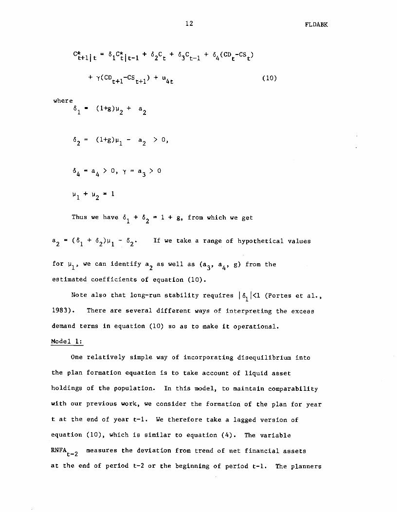
C*,41 = C51C*tlt_i+ ÷ S3C i + 54(C)t_CSt)
+ -y(CDt+i_cst÷i) + u4 (10)
where=
(l+g)u2 + a2
=(1+g)p1
—a2 > 0,
—a4 > 0, •y = a3 > 0
+ = 1
Thus we have + 2 = 1 + g, from which we get
a2 = ((S1+ 62)1 — 2 If we take a range of hypothetical values
for ji1, we can identify a2 as well as (a3, a4, g) from the
estimated coefficients of equation (10).
Note also that long—run stability requires I(St<l (Portes et al.,
1983). There are several different ways of Interpreting the excess
demand terms in equation (10) so as to make It operational.
Model 1:
One relatively simple way of incorporating disequilibrium into
the plan formation equation is to take account of liquid asset
holdings of the population. In this model, to maintain comparability
with our previous work, we consider the formation of the plan for year
t at the end of year t—l. We therefore take a lagged version of
equation (10), which is similar to equation (4). The variable
RNFA2 measures the deviation from trend of net financial assets
at the end of period t—2 or the beginning of period t—1. The planners
13 FLDABK
know this variable when they formulate the year t plan at the end of
t—l. Our plan formation equation would therefore be
Ctl = lC lit 2+ 2tl + + 4RNFA 2
+ 4t (11)
It is possible to estimate equation (11) together with equations
(l)—(3), and we call this Model I. It should be noted, however,
that since no current endogenous variables appear on the 1UIS of (11),
simultaneous estimation of the plan equation is unnecessary and will
yield the same results as estimation by OLS.
Model II:
We prefer to introduce disequilibrium explicitly into our model
in a manner consistent with the optimizing model developed above.
Taking again the formation of the plan for year t at the end of year
t—l we would have
C:Iti = 5lC_lit_2+ +
+ y(CD — CS) + 64(CDt 1— CSi) u4 (12)
As remarked above, it is computationally infeasible to include both
current and lagged excess demand terms, and we therefore seek proxies
for the lagged excess demand term. One possible measure of excess
demand in year t—l is the behavior of financial assets held by the
population, and we take the deviation from trend of net financial
assets at the end of year t—2 or beginning of year t—1, RNFAt2•
This gives the equation
14 FLDABK
=6C +C +Ctlt—l 1 t—1t--2 2 t—l 3 t—2
+ y(CD-CS) + S4RNFA 2 + u4 (13)
We call this Model ha. A slightly more general version of
(13) would allow CDt and CS to have unequal effects on
CJi , and we might enter this term as I1CDt + 2t We denote
this formulation as Model hib. Model ha is a special case of hib
with =12 i, and Model I is a special case of Model ha with
1 = 0.
This formulation also has the advantage of nesting Model I inside
Model II. The inclusion of actual or realized excess demand for
year t, which was queried above, is discussed further in Appendix B.
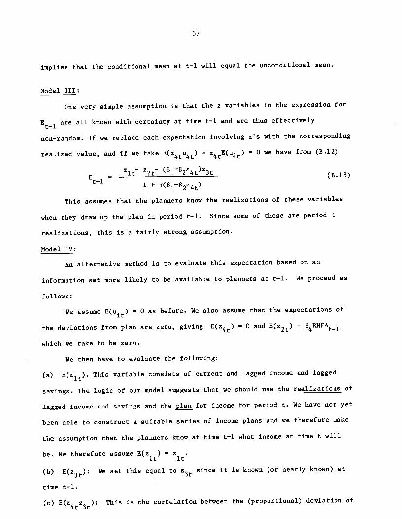
Models III and IV:
There are several ways in which the very strong informational
assumptions of Model II regarding (CDt — CS) might be relaxed.
One possibility would be to replace (CDt — CSt) by E 1(CDt — CS),the expectation of excess demand in year t, taken with respect to the
information available in year t—1, i.e. the predetermined variables in
the model. This variant is closer in spirit to the models which
feature in the rational expectations literature.
c*tlt_l
=5iC 1Jt2 + 2tl + cS3Ct 2 + 41'At_2 + yEi(CD_CS)
+ u4 (14)
In practice, one computes the likelihood function for this
variant by substituting the equations for CDt and CS in
Et_i(CD_CS). Appendix B considers assumptions which can be made
15 FLDABK
about the planners' expectations at time t—1 of the period t variables
in (CDt — CS). If the planners' expectations of the deviations of
NMP, D, etc., from their planned values in year t are taken to be what
subsequently occurred in year t, we have Model III. If, as might be
more plausible, the planners' expectations of these deviations are set
to zero, we have Model IV. Both models introduce restrictions
across the parameters of the equations of the full model.
Model V:
The strong informational requirements of Model I may be relaxed
in another way as well — by shifting the timing of the plan formation
equation one period forward relative to models I — IV. That is, we
return to the original timing of the plan equation as the plan for
t+l formed at the end of year t. We still face the problem of the
excess demand terms, and we seek use RNFAt_i as a proxy for
(CD+i — CS+i).Our equation for Model Va is then
C*11 = ÷ ts2ct + + —CS)
+ S4RNFAt + u (15)
In this model, the planners respond to current disequilibrium
(CD_CS) at the time they are making the plan for t+l. They also
respond to the deviation from trend of assets at the beginning of
period t, since this would be known at the beginning of year t.
This formulation of the model is to some extent more natural in that
it mimics the recursive nature of the planning process in which the
announced plan is determined before CDt and CS. It should
be noted, however that the equation for cannot be estimated
16 FLDABK
separately from (1)—(3) because of the presence of the endogenous Cand CDt_CSt (for details see appendix B).
Finally, we also allow for the possibility that the planners
respond in an asymmetric fashion to excess supply and to excess
demand. In Va we permit y = when CDt > CS and y = when
CD < CS , and we call this Model Vb.tt t
4. The Plan Data
We believe this to be the first study of the macroeconomic
behaviour of a CPE which includes consistent and comparable
time—series data on plans drawn from original sources. The data
themselves throw light on the abilities of the planners, events in
Poland, and planning as a process of prediction.
We have used plan data from the mid—1950s to 1980 on four time
series for this paper: consumption, NMP, gross investment and defence.
All variables are defined in constant zloties. The data on both
plans and realizations (actuals), together with detailed discussion of
methods and sources, are given in Portes et al. (1983). Table 1
shows the absolute deviations (in percent) of planned growth rates
from actual growth rates. Viewed in this way, the planners'
performance varies markedly over the period. The worst year in
terms of accuracy is 1972, when investment, which was planned to grow
at 9.6%, in fact grew at 23.017g. Thereafter actual investment was
t Our Model V is a more general version of what C—Q (p. 112) call"Model 3. We include in our plan adjustment equation the terms inboth their (4b) and their (4d), and we allow their coefficients todiffer from unity.
17 FLDABK
above plan until 1980. But the planners maintained a fair degree of
control. The 1978 plan reduced investment by 5.3%. Actual
investment rose slightly that year but fell in both 1979 and 1980.
The 1972 plan substantially underpredicted consumption as well.
Then, starting with the plan for 1976, the consumption plans were
underfulfilled for five successive years, with a remarkably large
shortfall in 1978. The NMP plans, too, were all underfulfilled from
1975 onwards, with a progressive deterioration in the performance
both of the planners and of the economy itself.
Of the 19 observations 1957—75, 9 consumption plans were
underfulfilled and 10 exceeded; for NMP, 7 and 12 fell in these
respective categories. Thus there was no clear pattern of excessive
pressure on the economy by the planners (or overoptimism), nor of
underestimating performance. From 1976 onwards, however, all
consumption and NMP plans were consistently underfulfilled, reflecting
the continuous deterioration of performance (as Mr. Gierek's economic
strategy disintegrated) and the planners' inability to come to grips
with it (Portes, 198lb). Investment and defence expenditure plans
show quite different pictures. The former were consistently
overfulfilled during the period (19 out of 24). The latter were
underfulfilled in all but two of the years 1957—67, overfulfilled in
all but one thereafter (through 1980)!
In relation to the mean planned growth rates, the average
absolute deviations given in Table 1 show a fair degree of planning
inaccuracy, if the plans are treated as predictions. Perhaps a better
measure of the predictive power of the planners Is in terms of levels.
Table 2 gives some comparisons. If the standard errors of the
deviations of planned levels from actuals are compared with the
18 FLDABK
standard deviations of the residuals from second—order autoregressive
processes fitted by OLS to the whole sample, we find the planners
out—perform the time—series regression for investment and defence but
not for consumption and NMP. Our consumption function [equation (1)]
estimated by OLS over the whole sample has a standard error of the
residuals under half that of the AR2 process and a third of the
"standard error of the plan'.
5. Results
The likelihood functions for the models specified in Section 3
are derived in Appendix B. We used the Davidon—Fletcher—Powell
algorithm to obtain maximum likelihood estimates, with numerical first
derivatives.
We tried variants of each of the models discussed. Model IV
performed poorly, so we do not report estimates from it.
Model lib (unequal ys) gives no significant improvement in the
likelihood over Ila (which is nested in it), whereas Va is rejected
against Vb. Thus we report results from Models I, ha, III and Vb.
All the results we give are from estimation with the restriction
= 1. Our theory regards C* as the ex ante supply plan, with
equation (2) representing the planners' adjustment of actual supply
away from that plan in response to new data. The planners may
consciously intend excess demand or excess supply. The restriction
assumes only that when they announce the plan, that is what they do
intend to offer to get their intended outcome. The restriction
= 1 is accepted by the data for the three models cited and for most
other runs.
The estimates are given in Table 3. We see immediately that a
19 FLDABK
likelihood ratio test rejects Model I against ha, in which it is
nested. On the whole, the correspondence with prior beliefs about
the coefficients is good. The demand equations for Model I
and III satisfied all conditions; those for Models ha and Vb give c
the right sign, but somewhat too small in absolute value (though not
significantly so), and both also make ct slightly but significantly
less than its theoretical value of unity. The long—run savings ratio
implied by the estimates for Model I is 2.1% in an economy growing at
5%.
The supply equation is less satisfactory; although the
equation's standard error is reasonable, the plan must be doing most
of the work in explaining supply (which is of course not inconsistent
with the deviations of actual from plan shown In Table 1). The NMP
deviation term is significant only for Models I and III, with the
correct sign. The defence expenditure term works well in all models.
But both and appear to take the wrong sign consistently. We
discuss this below.
The plan equation performs well. The second—order lag on
actual consumption, which we included because of previous work by
others and ourselves but does not appear in the theory of Section 3,
also does not appear in the data: is insignificant throughout.
The signs of other coefficients are as predicted, and the results seem
fairly stable; this equation is probably "best" in Model Vb. Note
that in Model I, the plan equation is decoupled" from the rest of the
model, and results obtained for it by OLS are identical within the
limits of numerical approximation to those shown in Table 3, which
confirms that our optimization programme is working properly. As in
20 FLDABK
our previous paper, we can calculate what constant growth rate of C
would be consistent with exact realization of plans in the estimated
version of equation (4). The answer ranges from 5.7% p.a. in Model
Vb to 7.4% in Model I, quite close to the observed 6.3% p.a. growth
of actual consumption in 1957—80.
As noted in Section 3, we can identify the parameters of our loss
function from the estimated plan—adjustment equation. The presence
of is a nuisance here, so we re—estimated subject to the
restriction that = 0, which was accepted for three of the four
models. With the normalization a1 = 1, we then find a3 not far from
0.5, a4 in the range 1.4—1.9, and —1.8 < a2< —0.7 for 0.25 0.75.
The smallest absolute values for a2 come in Model Va when p is large,
giving higher weight to C than to C1 in defining the path on
which the planners are trying to keep the economy. The growth rate on
that path is implied to lie between 5.7% and 7.2%. The signs of all
these parameters accord with our hypothesis, and the magnitudes seem
reasonable.
In addition to examining the point estimates, it is useful to
evaluate the model's ability to forecast actual consumption, C.
Ideally forecasts both from within and outside the sample are of
interest. In an ordinary linear regression model, it is natural to
compare the point estimate of a forecast with its confidence interval.
Some procedures, such as that of Chow, take into account the sampling
errors of the estimated coefficients. Others, such as that of
Davidson et al. (1978), confine themselves to the ratio of forecast
variance to residual variance.
In the present models, since the predicted value of C is the
output of a mm. function, it is not straightforward to calculate its
21 FLDABK
confidence interval. It appears that the simplest method of
evaluating the standard error of the predicted value of C is by
stochastic simulations (for details see Appendix A).
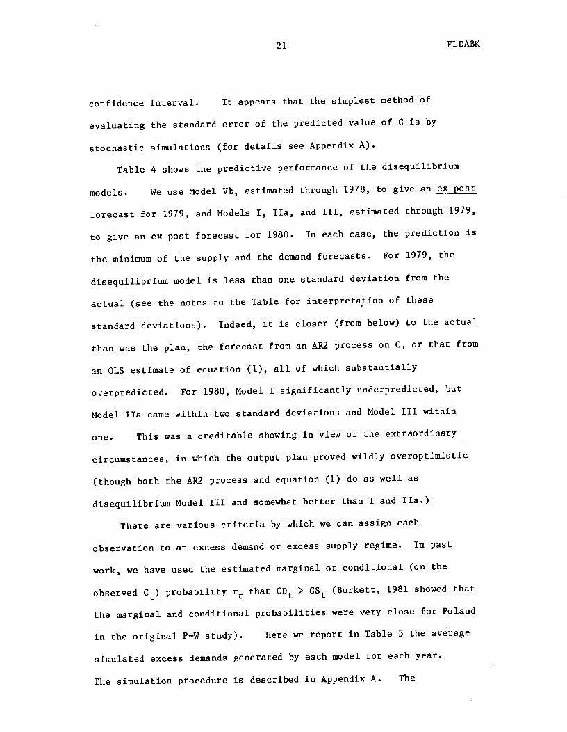
Table 4 shows the predictive performance of the disequilibrium
models. We use Model Vb, estimated through 1978, to give an ex post
forecast for 1979, and Models I, ha, and III, estimated through 1979,
to give an ex post forecast for 1980. In each case, the prediction is
the minimum of the supply and the demand forecasts. For 1979, the
disequilibrium model is less than one standard deviation from the
actual (see the notes to the Table for interpretation of these
standard deviations). Indeed, it is closer (from below) to the actual
than was the plan, the forecast from an AR2 process on C, or that from
an OLS estimate of equation (1), all of which substantially
overpredicted. For 1980, Model I significantly underpredicted, but
Model ha came within two standard deviations and Model III within
one. This was a creditable showing in view of the extraordinary
circumstances, in which the output plan proved wildly overoptimistic
(though both the AR2 process and equation (1) do as well as
disequilibrium Model III and somewhat better than I and ha.)
There are various criteria by which we can assign each
observation to an excess demand or excess supply regime. In past
work, we have used the estimated marginal or conditional (on the
observed C) probability that CDt > CS (Burkett, 1981 showed that
the marginal and conditional probabilities were very close for Poland
in the original P—W study). Here we report in Table 5 the average
simulated excess demands generated by each model for each year.
The simulation procedure is described in Appendix A. The
22 FLDABK
average excess demand for a given year is in practice positive if and
only if more than 50 of the 100 simulations for that year show excess
demand, but the correlation with the estimated conditional
probabilities is not perfect.t A more discriminating standard is set
by classifying an observation as excess demand or supply only if the
absolute value of the difference between the average simulated demand
and average simulated supply exceeds twice the standard deviation of
the simulated transacted quantity; in practice, this occurred only
when the proportion of cases in the favoured regime exceeded 75%.
A fairly consistent pattern averaged from applying all these
criteria with the three selected models. 1959, 1961, 1968, 1971—72,
1975, and 1979 were selected as years of clear excess demand. On the
other hand, 1958, 1960, 1962—64, 1967, and 1976—78 appeared to be
periods of excess supply In the consumption goods market. An overall
(though not unambiguous) judgment suggests 1965—66 were also excess
supply years, while 1974 and 1980 were probably excess demand. This
leaves 1957, 1969—70, and 1973 as impossible to classify. The models
themselves do not often disagree, though Vb differs distinctly from
the other three for 1957 and 1965—66, while Models I and III differ
from the other two for 1973—74.
This pattern Is broadly consistent with the development of the
Polish economy since the mid—1950s, and It is undoubtedly more
plausible than the classification (using estimated probabilities) in
Portes and Winter (1980). The dominance of excess supply in the
earlier years and excess demand in the 1970s accords with the
dominance of tight money wage control until Gierek replaced Gomulka at
t The estimated conditional rr suggest excess demand in 1963 and 1965under Model I, In 1965—67 under Model ha, and In 1967 under Model Vb,the end of 1970 (see the discussion in Portes, 1981b). 1959 saw aall of which show negative average simulated excess demand.
23 FLDABK
tremendous investment boom, 1968 political disquiet. The excess
supply shown in 1976—78 may reflect the plannerst efforts to satisfy
consumer pressures after the political explosion of mid—1976, while
tightening up their control of money wages and letting inflation
accelerate to soak up purchasing power.
The large estimated excess supply in 1978 appears to be the
consequence of a wildly overoptimistic plan, which our models do not
scale down sufficiently in response to the considerable shortfall of
NHP from its plan in 1978. This points out the relative weakness of
the supply equation, which may in part be due to the absence here of
any treatment of foreign trade and borrowing. For example, the
consistently "wrong" sign on 86 was explained in our earlier paper by
a supposed structural change around 1972, when the foreign borrowing
constraint was relaxed. Then investment need no longer have crowded
out consumption, and indeed the planners might have allowed for some
multiplier effects of investment on consumer demand and accommodated
them with additional imports.
The surprising but small negative coefficient on RNFAtin the
supply equation must be viewed in the light of the rather large
positive coefficient on the RNFA term in the plan—adjustment equation.
A sustained departure of NFA from trend will give a total effect on
supply, acting through C as well as directly, of
_____ — 84 + (81+820)o4
RNFA-
1+1
where 0 = (NMP— NNP*)/NMP*. With — 0.05 0 0.05, our estimates
give a range between 0.72 (in Model Vb) and 1.06 (in Model ha).
24
FLDABK
These suggest the planners do indeed seek market clearing: in
response to a sustained increase in household NFA, they would increase
the supply of consumption goods by roughly the same amount.
Judging only by the equation variance, the supply equation
appears to perform better than the demand equation in Models I and
III, whereas we have the converse in Models ha and Vb. This would
suggest that Models I and III would tend to put a higher proportion of
observations on or near the supply curve — i.e., more excess demand in
those models (see P—W, p. 151). Yet in fact the opposite is true,
which may suggest that the classification of observations between
regimes is not merely the consequence of the relative strength of the
specification of the demand and supply equations.
6. Conclusions
We believe we have taken substantial steps towards answering the
questions posed in Section 1 and demonstrating the applicability of
the C—Q model. Estimation has shown that it is both feasible and
informative to use plan data, and to model the regularities in the
process of plan construction. The plan depends upon planned and
actual consumption and excess demand. These announced plans are
embodied in a supply function which reflects, in addition, unforeseen
subsequent developments in the economy. The planners do appear to
try to adjust announced plans and actual supply in order to reduce
excess demand. The disequilibrium macroeconomic framework, with
fixed prices and planned quantities, can be estimated for centrally
planned economies and seems to provide insight into their behaviour.
The pattern of excess demands revealed by the data appears broadly
consistent with economic events in Poland.
25
FLDABK
We have data sets which permit application of the model to at
least two other countries, and there are various extensions of the
analysis which we shall explore in future work. Moreover, we intend
to apply a similar approach to other macro variables and markets —
e.g., investment, the labour market or NMP itself.
The deviation for a variable X is defined as 100(X _X*)/X, where X
t t t—1 t
is the actual and X* = X is the planned level of the variable Xt tgt—i
for period t.
27
TABLE 2
Perforiiauce of Plans, 1957—80
(billion zioties, constant prices of 1971)
Sample mean 448.88 836.73 270.85 31.87
Standard deviation ofplan from actual 17.72 31.80 14.78 1.09
Standard error ofresidual from AR2process 12.38 21.86 17.91 1.95
Standard error ofresidual from OLSestimates:
CD [equation (1)] 5.26
CS [equation (2)] 11.61
Notes:
A second—order autoregressive (AR 2) process was fitted to theseries of actual data, and we cite above the standard error ofthe residuals from this form of "explanation".
All estimates are ML estimates. There are no small sample
adjustments.
28
TABLE 3
Estimates of Disequilibrium Models, Poland 1957—80
NotesAsymptotic standard errors in parentheses. The sample mean ofC was 448.88.
29
TABLE 4
Comparative Predictions
1979 1980
Actual 794.82 817.97
Plan 803.87 840.44
AR2 812.61 815.44
CD function (OLS) 800.93 815.29
Disequilibrium estimates 790.32 ( (1) 799.11
[mm (CD, Cs)] (ha) 812.97
815.51
Standard deviations of 6.66 r (I) 6.99
disequilibrium estimatesin simulations (ha) 2.69
hhI)3.50
Notes
The second—order autoregressive process (AR2) in C and theconsumption function (our CD, estimated by OLS) are estimated on1957—78 for the 1979 prediction and 1957—79 for the 1980prediction. The disequilibrium model prediction for 1979 isfrom model Vb run through 1978, while those for 1980 are frommodels I, ha and III, respectively, each run through 1979.The last line is the standard deviation of Cs from the stochasticsimulations (see Appendix A). Normally, would compare theforecast error with the simulated error of the equation; here,however, we do not have values of the simulated predictionerrors, but we do have the standard error of the transacted
quantity.
30
TABLE 5
Average Simulated Excess Demands (Per Cent)
Model I Model ha Model III Model Vb
1957 3.0 3.7 0.7 —3.6
1958 —4.1 —1.8 —2.5 —3.9
1959 0.8 0.7 —0.8 1.0
1960 —6.8 —5.5 —5.2 —4.4
1961 5.1 2.2 1.7 1.4
1962 —4.1 —3.1 —2.8 —2.0
1963 —0.3 —1.5 —0.8 —0.6
1964 —4.2 —2.5 —3.1 —1.6
1965 —1.1 —0.8 —1.0 1.8
1966 —3.5 —2.0 —3.0 1.0
1967 —3.0 —1.1 —2.1 —0.7
1968 0.4 1.8 0.5 2.5
1969 —0.9 1.6 —0.8 0.2
1970 —0,2 0.9 0.1 —1.0
1971 4.5 3.8 2.2 2.5
1972 0.7 5.0 0.9 7.0
1973 —3.0 1.8 —2.3 2.7
1974 —0.9 3.6 —0.3 1.2
1975 1.0 2.2 —0.4 2.8
1976 —1.0 -0.8 —2.4 —2.9
1977 —1.5 —1.3 —2.6 —0.1
1978 —10.7 —7,1 —7.2 —8.7
1979 1.5 0.4 0.4 1.2
1980 1.2 —0.1 0.5 1.2
31
FLDABK
References
Burkett, J., 1981, Marginal and conditional probabilities of excessdemand, Economics Letters 8, 159—162.
Charemza, W., and R. Quandt, 1982, Models and estimation ofdisequilibrium for centrally planned economies, Review ofEconomic Studies 49, 109—116.
Davidson, J., D. Hendry, F. Srba and S. Yeo, 1978, Econometricmodelling of the aggregate time—series relationship betweenconsumer's expenditure and income in the United Kingdom,Economic Journal 88, 661—692.
Cacs, L. and M. Lacko, 1973, A study of planning behaviour on thenational—economic level, Economics of Planning 13, 91—119.
Portes, R., 1981a, Macroeconomic equilibrium and disequilibrium incentrally planned economies, Economic Inquiry 19, 559—578.
Portes, R., 1981b, The Polish Crisis (London, RIIA).
Portes, R., R. Quandt, D. Winter, and S. Yeo, 1983, Planning theconsumption goods market: Preliminary disequilibrium estimatesfor Poland 1955—80, NBER Working Paper no. 1076, forthcoming ina conference volume edited by P. Malgrange and P.—A. Muet
(Blackwell).
Portes, R., and D. Winter, 1977, The supply of consumption goods incentrally planned economies, Journal of Comparative Economics 1,
35 1—365.
Portes, R., and D. Winter, 1980, Disequilibrium estimates forconsumption goods markets in centrally planned economies, Review
of Economic Studies 47, 137—159.
Quandt, R., 1981, Autocorrelated errors in simple disequilbriummodels, Economics Letters 7, 55—61.
Yeo, S., 1983, Some simple models of plan adjustment, BirkbeckDiscussion Paper in Economics (forthcoming).
32
Appendix A: Description of the Stochastic Simulations
We performed stochastic simulations for several of the models.
The basic steps in these simulations are as follows:
1) Define the vector 4 = as (CD,CSt,C) for
models I to IV and as (CD,CS,C+i) for model V. We then can
write the structural equations (excluding the nun condition) as
Ay w ÷ u (A.1)
where w = (wit,w2,w4) represents the exogenous and predetermined
variables and their coefficients from the right hand sides of these
equations, u = (ui,u2,u4) the corresponding error terms and where
A is a square matrix of coefficients.
2) For each observation, t = 1, ..., T and for each simulation i
substitute in A the values of the estimated coefficients and
substitute in w the estimated coefficients of the predetermined and
exogenous variables and the values of these variables for the tth
observation. Note that A and w do not vary across the simulations i.
3) For each observation t = 1, ..., T, and for each simulation
i = 1, ... 100 generate three independent normal variables with mean
zero and variances a, o, a, where the latter are the estimated
error variances; denote these simulated normal errors by u for
simulation 1.
4) Obtain simulated solutions by solving
Al(w + ui) (A.2)
5) Obtain simulated values of the actual level of consumption
and the simulated forecast error for simulation I from
Cs = inin(y8 ,y5 ) (A.3)ti iti 2ti
f = C —C1 (A.4)
33
6) Repeat steps 2 through 5 for simulations I = 1, ... 100
7) For each t = 1, ... T compute the arithmetic means and
standard deviations of y , C and f across the simulations I.
It is possible to introduce three sources of random variation in
a stochastic simulation: variations in the estimated coefficients, in
the exogenous variables and in the equation error terms. We have only
introduced variation in the error terms u1 in the work reported here,
but we hope to investigate full stochastic simulations in later work.
34
Appendix B: The Likelihood Functions
Models I and II:
It is convenient to derive the likelihood function for Model lIb first,
since the results for models I and [Ia then follow as special cases.
Model [lb can be written
CD= + ui (B.l)
CS =1+ + (B.2)
C = mm (CDt,CS) (B.3)
C11 = z3t + y1CD + y2CS + U4 (B.4)
where C1 represents the plan for period t formulated in t—l. For
convenience of notation this is written below as . We have also
z1 = ciDNFAt_i + cz2DYD + a3YDti
Z2= 84t—1 + +
23t = + cS2Ct_i + 3Ct2 + S4RNFAt2
(NMP—NP)/NMP
We assume that ui, u2 and u4 are serially independent normal variates
with a diagonal covariance matrix. The pdf of CDt, CS, C is immediate from
(B.1) to (B.4):
—
f(CD ,CS ,C*) = (B.5)t t t 3/21Tj 010204
÷
The pdf of the observable random variables C, C is
h(C,C) = jf(Ct,CS,C)dCS + I f(CD,C,C)dCD (B.6)
It is easy to show by completing the square that the integrals in (B.6) can be
obtained as
exp (— —
204
Ii —f f(C ,CS ,C*)dCS =t t t t '222c 27ra1i(a4+12a2)
1 (C—zi)2 Bt —
exp— +21 2
1 1
Ii -f(CD ,C ,C*)dCD =t t t t
2ia2/(a+ic1)
(C—z '2I lflt 5t'
exp— —I +
Z5 = Z2 +
z =C*_vC —z6t t '1 t 3t
z7t= — '2t — 3t (B.9)
A = a4ZS +
t
a2 2 +B = 45 °26t _________t
22 22
1 2 + 22 2 + y2a2
where ( ) is the standard normal distribution function. The log—likelihood
model lib is then L = log h(Ct,C*).t tThe likelihood function for model I can be obtained by taking = 2 = 0,
and the likelihood function for model ha by taking 2 '
Models Involving Expected Excess Demand (III and IV):
The likelihood functions for the models involving expected excess demand
in the plan adjustment equation can be obtained as follows:
35
ICt
(B.7)
jJ
(B.8)
jwhere
G
x
1
x 1—
x
x-
2a1lZ722
I
a2z21 7t
1
F =
= az +
and
for
36
The structural equations include (B.l), (B.2), (B.3), but the plan
equation is now
Ck1= z3 + yEt_i(CDt—CSt) + u4 (B.1O)
where z1, z2, z3, z and z5 are as defined for Model II. For simplicity we
again denote C1_1 by C and Et_i(CD_CS) by Er_i in what follows. Because
Et_i itself depends only on predetermined and exogenous variables, the density
function of the observable random variables is the product of the pdf for a
simple disequilibrium model corresponding to (B.1), (B.2) and (B.3), and the
pdf of the single equation model given by (B.1O):
1 1 (C—z3_yEti)2f(C ,C*) = exp I
— — x (B.11)t2
J
exp ! (ct_z5)2 x — [_1
2 J [ JJ1
exp (_ (c_zi)2 — [ct_z5t2 o J [ 2
It should be noted that the model does not decouple into two independent
sub—models because in general, Et_i will depend on the parameters in the other