( Ml I I

ricultural •

onom1cs Report REPORT NO. 492 NOVEMBER 1986

MAXIMUM (MINIMUM) BID (SELL) PRICE MODELS FOR LAND WHEN DEPRECIABLE ASSETS

ARE INCLUDED IN THE TRANSACTION

G l1\:-!,-.J NI C.L ""' :Y' l C .· AGRICULTURA~ ~OMICG

LID~·

/ ~~' ) .07 ~ ~ .. ;~ .~J

By:

Lindon J. Robison Steven R. Koenig Myron P. Kelsey

r-.. partment of _......,

"ricultural Economic J Lr 'CHIGAN STATE

HVERSITY. East Lansing

MAXIMUM (MINIMUM) BID (SELL) PRICE MODELS

FOR LAND WHEN DEPRECIABLE ASSETS

ARE INCLUDED IN THE TRANSACTION

by

Lindon J. Robison, Steven R. Koenig, and

Myron P. Kelsey

ABSTRACT

MAXIMUM (MINIMUM) BID (SELL) PRICE MODELS FOR LAND WHEN DEPRECIABLE ASSETS ARE INCLUDED IN THE TRANSACTION*

by

Lindon J. Robison, Steven R. Koenig, and

Myron P. Kelsey**

This paper constructs maximum bid and minimum sell models to be used for the

analysis of purchases and sales of real estate. Real estate includes land and

depreciable assets sold or purchased together. The models in this paper extend

those developed for land by Robison and Burghardt . Including depreciable assets

together with the purchase and sale of land allows a more complete analysis of

the role of taxes including the effects of the 1986 tax law.

*Michigan Agricultural Experiment Station Journal Article No. 12186.

**Lindon J. Robison and Myron P. Kelsey are, respectively, Associate Pro­fessor and Professor in the Department of Agricultural Economics, Michigan State University, East Lansing, Michigan. Steven R. Koenig was a graduate student at Michigan State University and is now an Agricultural Economist with the Economic Research Service of the U.S. Department of Agriculture.

TABLE OF CONTENTS

Introduction . . . . . . . •

Definitions and Notations ••

Tax Implications of Owning Depreciable Assets .•

The Maximum Bid Price Model (V) .••

The Minimum Sell Price Model (Vs) ..

Building Financial Considerations Into Maximum Bid and Minimum Sell Price Models.

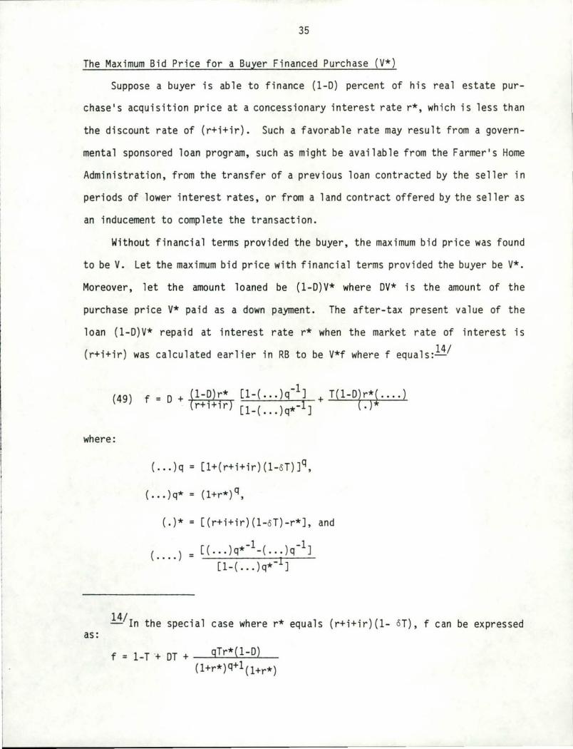
The Maximum Bid Price for a Buyer Financed Purchase (V*).

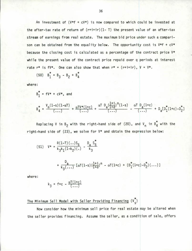
* The Minimum Sell Model with Seller Providing Financing (Vs)

Minimum Sell Model with a "Due on Sale" Clause with No Seller Financing (V~). . . ••.

Empirical Results .•

Epilogue •

References

Page

1

3

7

16

24

34

35

36

42

45

51

53

MAXIMUM (MINIMUM) BID (SELL) PRICE MODELS FOR LAND WHEN DEPRECIABLE ASSETS ARE INCLUDED IN THE TRANSACTION

by

Lindon J. Robison, Steven R. Koenig, and

Myron P. Kelsey

Introduction

Several studies have examined the break-even price for land, including Lee

and Rask's, Baker's, and Robison and Burghardt's. Capital budgeting books,

including Bierman and Schmid's, Aplin et al., and Canada and White's, have been

written about methods which can be used to value depreciable assets. But fre­

quently land and depreciable assets are sold together as real estate. The

purpose of this paper is to develop general methods for finding minimum sell and

maximum bid prices for real estate.

The development of the models follows capital budgeting principles suggest­

ed by Robison and Burghardt and which are generally accepted by others.l/ The

land models developed by Robison and Burghardt also form the foundations for the

land portion of the real estate models developed here. And like their models,

the one developed in this paper includes such features as real estate, income and

capital gains taxes, transactions costs, holding period length, and financial

arrangements. Moreover, the models are developed from both the break-even per-

spective of the buyer and the seller.

l/The five principles suggested by Robison and Burghardt are: (1) the homogeneity of measurements principle; (2) consistency in timing principle; (3) opportunity cost principle; (4) the life of the asset principle; and (5) the total cost and returns principle.

2

The need for a paper such as this and the models which it develops is

because few transactions involve bare land. Most generally, a depreciable asset

is included in the sale of the land. Drainage tiles, buildings, machinery,

wells, sump pumps and lift stations, fences, mineral rights, and storage facili-

ties are all examples of depreciable assets which may be included in the sale of

land.

Including a depreciable asset with the purchase of a nondepreciable asset

land complicates maximum bid and minimum sell price calculations in two fundamen-

tal ways. First, tax provisions require that the purchase price of real estate

be divided between the depreciable and nondepreciable assets. The depreciable

and nondepreciable assets are then taxed at different rates. Second, variables

such as inflation may have differing effects on depreciable and nondepreciable

assets leaving inflation's overall impact ambiguous whereas before it could be

unambiguously signed. Consequently, capital gains may accumulate at a rate

different than the rate of increase in income.

In what follows, extensions of the Robison and Burghardt (RB) models are

developed to calculate maximum bid and minimum sell price models for real estate.

The models developed in this paper are consistent with the five principles they

suggest for building present value models and consistent with the 1986 tax laws.

This paper does not, however, generate formulas for all tax depreciation schemes

for depreciable assets which may arise. Instead, we present results consistent

with the straight-line depreciation method.'!:./

Finally, the discount rate is generalized to alternatively reflect returns

consistent with tax-free bonds, financial instruments whose earnings are taxed

at the income tax rate, or investments whose effect ivce tax rate

'!:./A depreciable asset is defined in this paper as any asset whose value creates a tax shield resulting from its book value depreciation.

3

falls in between zero and the income tax rate including land and depreciable

asset purchases. In an effort to avoid confusion, notation used by RB i·S

continued here with minor exceptions. The next section begins by restating those

definitions.

Definitions and Notations

Maximum (minimum) bid (sell) price models are one type of model included in

the general class of present value models. Present value models consist of three

parts: {l) the asset's bid (sell) price valued in current period dollars; (2) a

stream of future costs and returns attributable to the acquisition use and

maintenance of the asset; and (3) the discount rate which discounts future cash

flows to their current period equivalent. If two of the three elements of the

present value model are known, the third can be found. Or if all three are known,

the difference between the asset's bid (sell) price and the discounted costs and

returns can be calculated. This model, a net present value model, indicates

whether an investment earns a return greater than, equal to, or less than the

discount rate. The sign of the difference, a net present value, is often used as

an investment criterion.

An asset's internal rate of return (IRR) can be used as another investment

criterion when the asset's price and future cash flows are known. An invest-

ment's IRR is the discount rate or rate of return associated with the investment

which equates the asset's price and future cash flow. One may compare the IRRs

on similar investment opportunities and use the difference as an acceptance

criterion. It, of course, goes without saying that multiple IRRs or no IRR at

all may exist.1/

.~/conditions under which the IRR is unique is summarized in Brealey and Myer.

4

If the discount rate and the future cash flows are known, one can solve for

the current period sum of the discounted cash flows and refer to the result as

maximum (minimum) bid (sell) model. The term maximum (minimum) bid (sell} model

is appropriately named because it represents an equality of attractiveness be­

tween the asset being purchased (or sold) and an alternative investment whose ,.

internal rate of return is described by the discount rate. Thus, the discount

rate in the maximum (minimum) bid (sell) model is also an internal rate of

return.

Maximum bid (minimum sell) price models provide information which can be

used as a decision criterion for investment problems . If the maximum (minimum)

bid (sell) price is greater (less) than the price for which for the asset can be

purchased (sold), the investment (disinvestment) should be undertaken since the

investment would then earn a rate in excess of the discount rate. But, all three

elements of the present value problem must be known before a decision can be

made. Thus, the maximum bid (minimum sell) models are designed to find indiffer-

ence conditions; they do not by themselves provide decision criteri a.

Maximum bid and minimum sell price models have many of the same cost and

return considerations except they appear in different ways. For example. the

maximum bid price for a potential buyer depends on the cost of acquiring the

asset, expected returns and costs, tax considerations, and expected future sales

prices (which, in turn, depends on expected income and costs of the next buyer).

Thus, in the 1 ong run, every rea 1 estate purchaser eventually becomes a rea 1

estate seller. And every seller weighs the sell opportunities with the benefits

from continued ownership.

Some of the variables influencing buyers and sellers of bare land are:

r = a real rate of return available to the firm on its investments,

T = a constant proportional income tax rate paid by the firm,

5

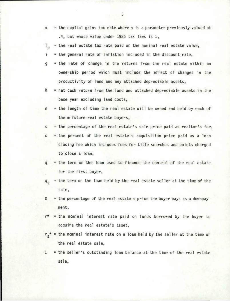
a = the capital gains tax rate where a is a parameter previously valued at

.4, but whose value under 1986 tax laws is 1,

TP =the real estate tax rate paid on the nominal real estate value,

i = the general rate of inflation included in the discount rate,

g = the rate of change in the returns from the real estate within an

ownership period which must include the effect of changes in the

productivity of 1 and and any attached depreciable assets,

R = net cash return from the 1 and and attached depreciable assets in the

base year excluding land costs,

n = the length of time the real estate will be owned and held by each of

the m future real estate buyers,

s = the percentage of the real estate's sale price paid as realtor's fee,

c =the percent of the real estate's acquis i tion price paid as a loan

closing fee which includes fees for title searches and points charged

to close a loan,

q = the term on the loan used to finance the control of the real estate

for the first buyer,

qs = the term on the loan held by the real estate seller at the time of the

sale,

D = the percentage of the real estate's price the buyer pays as a downpay-

ment,

r* = the nominal interest rate paid on funds borrowed by the buyer t o

acquire the real estate's asset,

r * = the nominal interest rate on a loan held by the seller at the time of s

the real estate sale,

L = the seller's outstanding loan balance at the time of the real estate

sale,

6

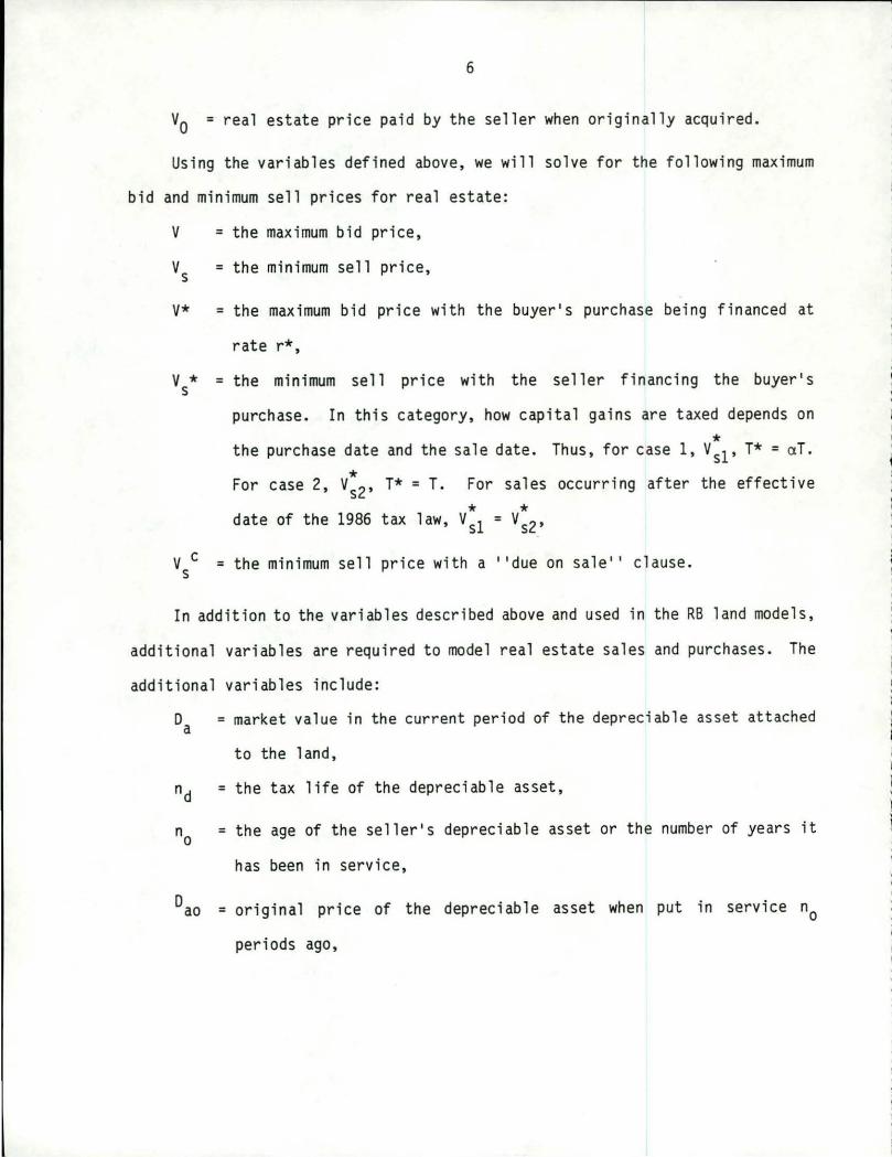
v0 = real estate price paid by the seller when originally acquired.

Using the variables defined above, we will solve for the following maximum

bid and minimum sell prices for real estate:

V = the maximum bid price,

Vs = the minimum sell price,

V* =the maximum bid price with the buyer's purchase being financed at

rate r*,

V * = the minimum sell price with the seller financing the buyer's s

purchase. In this category, how capital gains are taxed depends on

* the purchase date and the sale date. Thus, for case 1, Vsl' T* = aT.

* For case 2, V s2, T* = T. For sales occurring after the effective

* * date of the 1986 tax law, vsl = vs2'

V c =the minimum sell price with a 1 'due on sale' 1 clause. s

In addition to the variables described above and used in the RB land models,

additional variables are required to model real estate sales and purchases. The

additional variables include:

Da = market value in the current period of the depreciable asset attached

to the land,

nd = the tax life of the depreciable asset,

n0

=the age of the seller's depreciable asset or the number of years it

has been in service,

0ao = original price of the depreciable asset when put in service n0

periods ago,

7

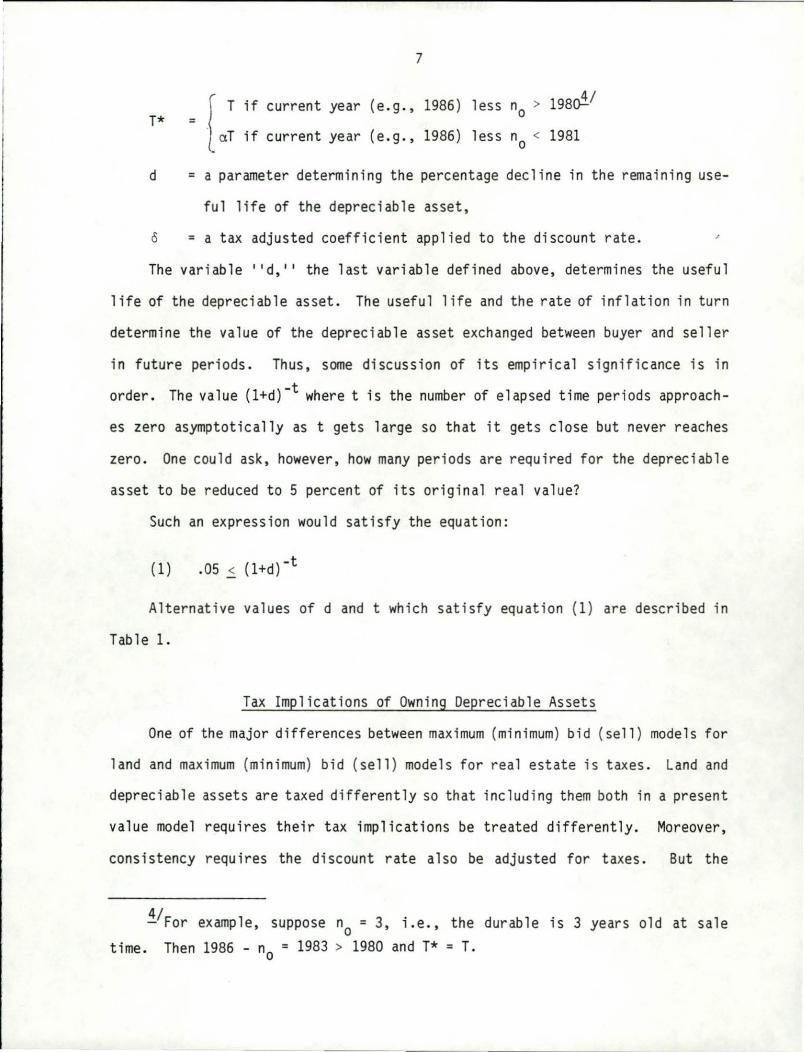
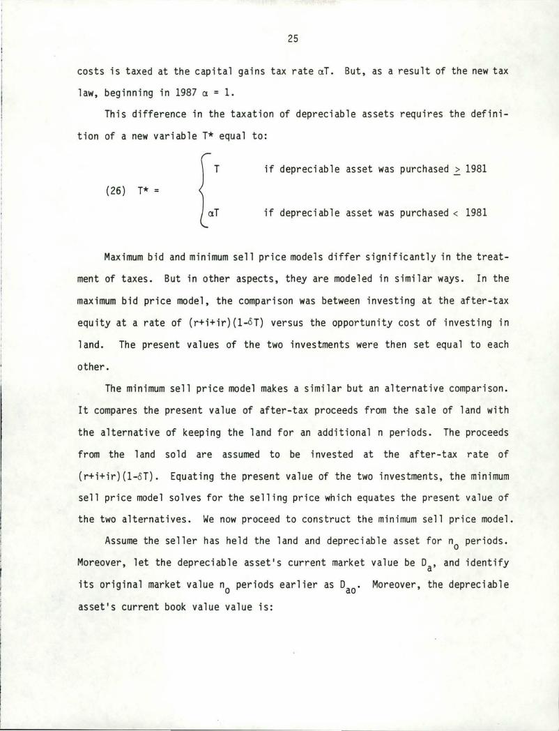
f T if current year (e.g., 1986) less no > 1980~/ T* =

_ aT if current year (e .g., 1986) less no < 1981

d = a parameter determining the percentage decline in the remaining use-

ful life of the depreciable asset,

= a tax adjusted coefficient applied to the discount rate.

The variable 11 d, 11 the last variable defined above, determines the useful

life of the depreciable asset. The useful life and the rate of inflation in turn

determine the value of the depreciable asset exchanged between buyer and seller

in future periods. Thus, some discussion of its empirical significance is in

order. The value (l+d)-t where t is the number of elapsed time periods approach -

es zero asymptotically as t gets large so that it gets close but never reaches

zero. One could ask, however, how many periods are required for the depreciable

asset to be reduced to 5 percent of its original real value?

Such an expression would satisfy the equation:

(1) .05 ~ (l+d)-t

Alternative values of d and t which satisfy equation (1) are described in

Tab 1 e 1.

Tax Implications of Owning Depreciable Assets

One of the major differences between maximum (minimum) bid (sell) models for

land and maximum (minimum) bid (sell) models for real estate is taxes. Land and

depreciable assets are taxed differently so that including them both in a present

value model requires their tax implications be treated differently. Moreover,

consistency requires the discount rate also be adjusted for taxes. But the

~1For example, suppose n0

= 3, i.e., the durable is 3 years old at sale time. Then 1986 - n

0 = 1983 > 1980 and T* = T.

8

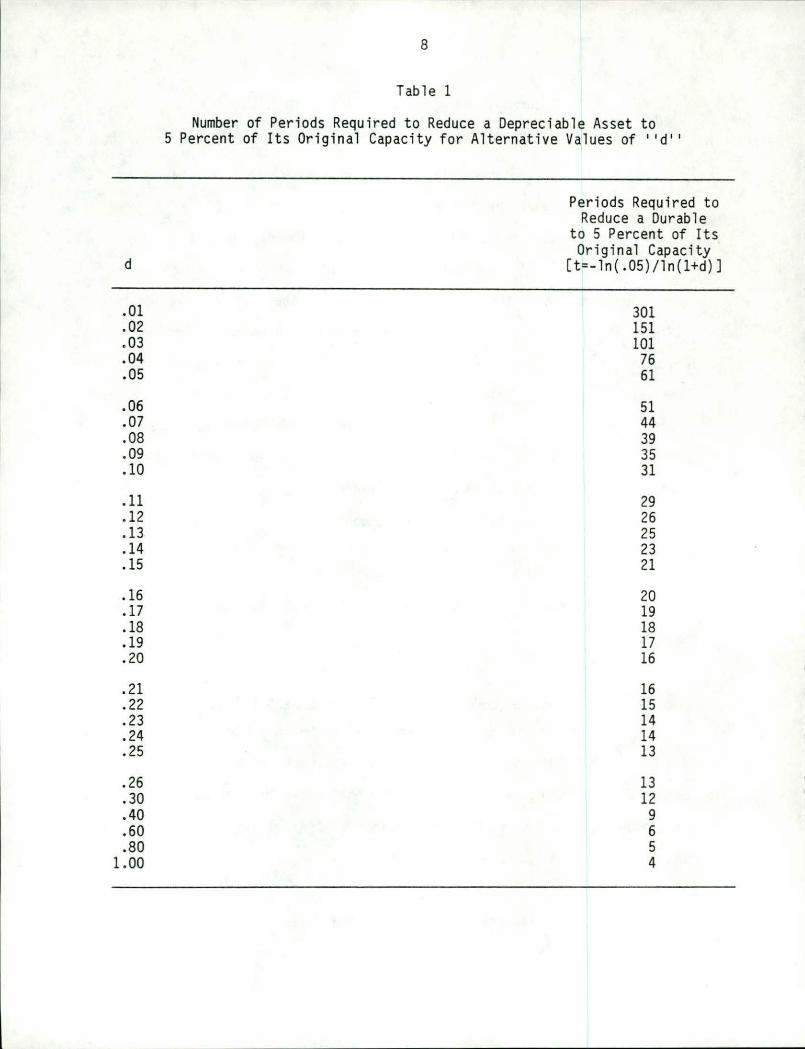
Tab 1 e 1

Number of Periods Required to Reduce a Depreciable Asset to 5 Percent of Its Original Capacity for Alternative Values of ''d' '

Periods Requi r ed to Reduce a Durable

to 5 Percent of Its

d Original Capacity

[t=-ln(.05)/ln(l+d)]

.01 301

.02 151

.03 101

.04 76

.05 61

.06 51

.07 44

.08 39

.09 35

.10 31

.11 29

.12 26

. 13 25

.14 23

.15 21

.16 20

.17 19

.18 18

.19 17

. 20 16

.21 16

.22 15

.23 14

.24 14

.25 13

.26 13

.30 12

.40 9

.60 6

.80 5 1.00 4

9

question is at what tax rate should the discount rate be adjusted? The answer is

it all depends on what is the next best investment opportunity available to the

firm?

If the next best investment opportunity is a financial instrument whose

returns are taxed at the firm or individual's income tax rate T, then the

appropriate tax adjustment is to multiply the rate of return by (1-T ) . If the

next best investment is a tax-free bond, then the appropriate discount rate is

the rate of return on the bond unadjusted for taxes. Finally, if the next best

investment opportunity is an asset whose returns are partially shielded from

income tax, the appropriate tax rate by which the discount rate is adjusted is

(1-oT) where 0 < o < 1. Of course, setting o = 1 or o = 0, models the tax

adjustment required for financial instruments and tax-free bonds, respectively.

Having introduced taxes into the discount rate, attention is now directed at

capturing the tax implications of an investment when a depreciable asset is

attached to land.

The first step in calculating the tax implication resulting from including

depreciable assets in the purchase of real estate is establishing the depreciable

asset's beginning book value. This value, Da, should correspond to the market

value of the depreciable asset and legally (although not always done in practice)

must be agreed on by the se 11 er and the buyer. The buyer is then a 11 owed to

prorate closing fees of c percent of the purchase price to the depreciable asset

establishing a cost basis or beginning book value of (l+c)Da . The periodic tax

shield when the depreciable life of the durable is nd and straight-line deprecia­

tion is used then becomes (l+c)Da/nd . .?/

.§/rt is recognized that for some depreciable assets, ACRS or other deprecia­tion methods would be used. Model limitations preclude us from generalizing the method of tax depreciation. Instead, nd can be altered to approximate the actual tax depreciation schedule followed.

10

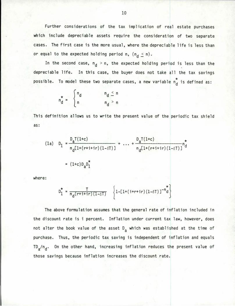
Further considerations of the tax implication of real estate purchases

which include depreciable assets require the consideration of two separate

cases. The first case is the more usual, where the depreciable life is less than

or equal to the expected holding period n, (nd _:: n) .

In the second case, nd > n, the expected holding per iod is less than the

depreciable life. In this case, the buyer does not take all the tax savings

* possible. To model these two separate cases, a new variable nd is defined as:

* n = d

n < n d -

n > n d

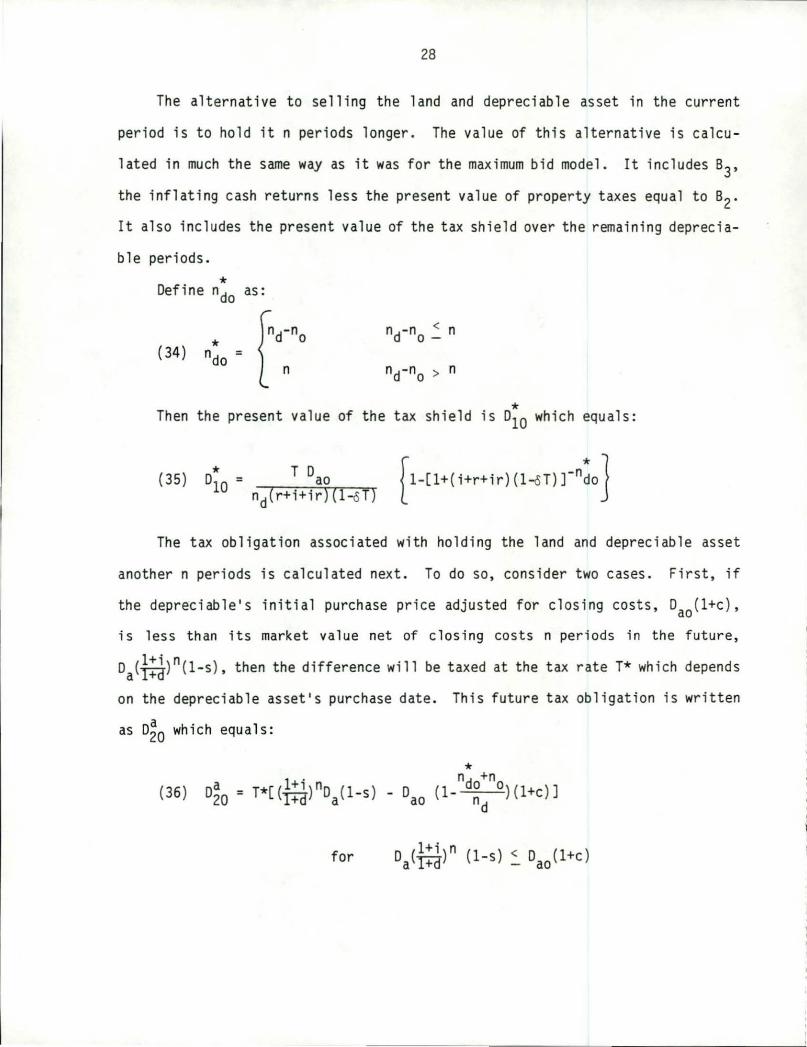
This definition allows us to write the present value of the periodic tax shield

as:

DaT(l+c) D T( 1 +c) * (la) 01 = + ••• + a n

nd[l+(r+ i+ir)(l-oT)] nd[l+(r+i+ir)( l-oT)] d

* = (1 +c) DaDl

where:

* T ! 1-[1+( i+r+ir) (1-0T) r"~ 1 01 = nd(r+i+ir)(l-oT)

The above formulation assumes that the general rate of inflation included in

the discount rate is i percent. Inflation under current tax law, however , does

not alter the book value of the asset Da which was established at the time of

purchase. Thus, the periodic tax saving is independent of inflation and equals

TD/nd. On the other hand, increasing inflation reduces the present value of

those savings because inflation increases the discount rate.

11

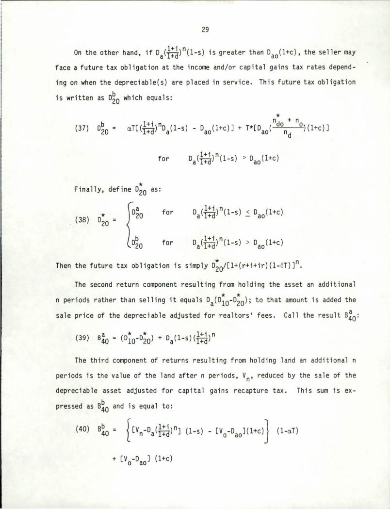
In addition to the inflationary effect on the tax shield, inflation compli­

cates matters at the end of n periods when the land and the attached depreciable

assets are sold. If the sale price of the depreciable asset exceeds the depreci­

ated book value, the difference is subject to depreciation recapture provisions.

An ordinary income tax obligation on the difference is imposed up to the original

purchase price. If the depreciable asset is sold at an amount exceeding the

original purchase price, previous to 1987, that difference between the current

and original price is taxed at the capital gains rate.

Tax laws passed in 1986 increase the capital gains tax rate to T. This

change will affect tax write-offs when the sale price of the depreciable asset

exceeds its original book value. This condition is most likely to be satisfied

during periods of high inflation rates; that is, when the inflation rate exceeds

the productivity decay of the depreciable asset (i > d).

At the time of the sale, the buyer and seller must agree to the current

value of the depreciable asset. From a tax standpoint, it is in the seller's

best interest to allocate a small portion of the sale to the depreciable asset.

This approach allows the seller to mitigate the effects of recapture provisions

which tax the difference between the depreciable asset's adjusted book value at

the time of the sale and the asset's sale price in the nth period. On the other

hand, it is in the buyer's best interest to allocate a larger portion of the

purchase price to the depreciable asset since establishing a large book value

increases the value of future tax shields.

To model real estate transactions requires that the buyer and seller agree

to the sale price of the depreciable asset. This is done in our model by

discounting the original purchase price of the depreciable asset, Oa, at the rate

at which its useful life declines, d, and inflating it at the rate of inflation

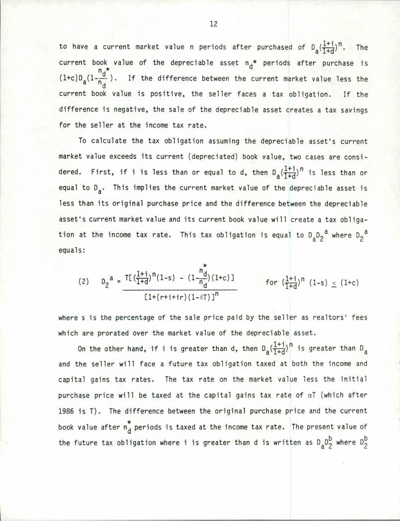
i. Thus, a depreciable asset whose original purchase price was Da, is calculated

12

l+i n to have a current market value n periods after purchased of Da(-I+cr) . The

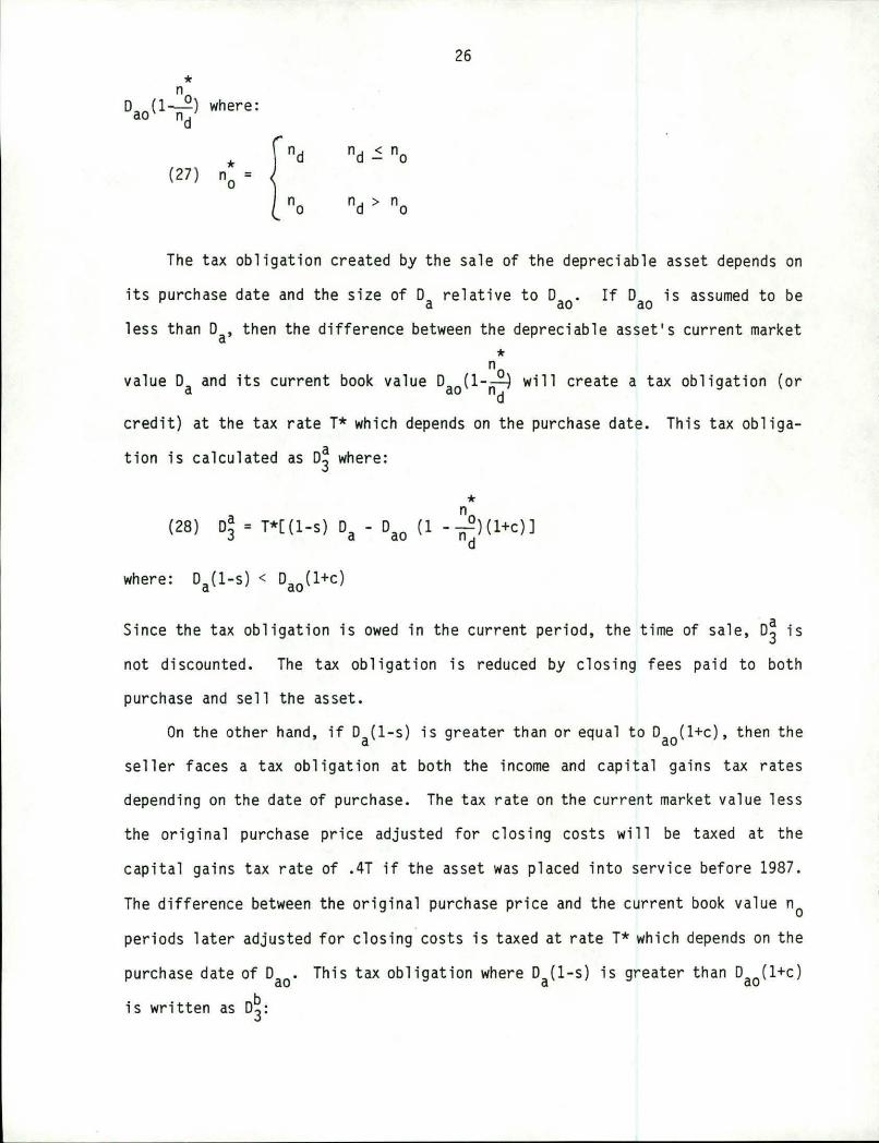
current book value of the depreciable asset n/ periods after purchase i s n *

(l+c)O (1-.!!. ). If the difference between the current market value less the a nd current book value is positive, the seller faces a tax obligat ion . If the

difference is negative, the sale of the depreciable asset creates a tax savings

for the seller at the income tax rate.

To calculate the tax obligation assuming the depreciable as set's current

market value exceeds its current (depreciated ) book value, two cases are cons i ­

dered. First, if i is less than or equal to d, then Da (f:d )n i s less than or

equal to Oa. This implies the current market value of the depreciable asset i s

less than its original purchase price and the difference between the depreciable

asset's current market value and its current book value will create a tax obliga­

tion at the income tax rate. This tax obligation i s equal to oao2a where o2a

equals:

(2) D a 2

[l+(r+i+ir )( l-oT) ]n

for (f :d )n (1-s ) < (l+c)

wheres is the percentage of the sale pri ce paid by the sel l er as real t ors ' fees

which are prorated over the market value of the depreciable as set.

l+i )n . On the other hand, if i is greater than d, then Da(T+d i s greater than Da

and the seller will face a future tax obligati on taxed at both the i ncome and

capital gains tax rates . The tax rate on the market value l ess t he in iti al

purchase price will be taxed at the capital gains tax r ate of aT (which after

1986 is T) . The difference between the original purchase price and the current

* book value after nd periods i s taxed at the income tax rate. The present value of

the future tax obligat ion where i is greater than d is written as Dao~ wher e D~

13

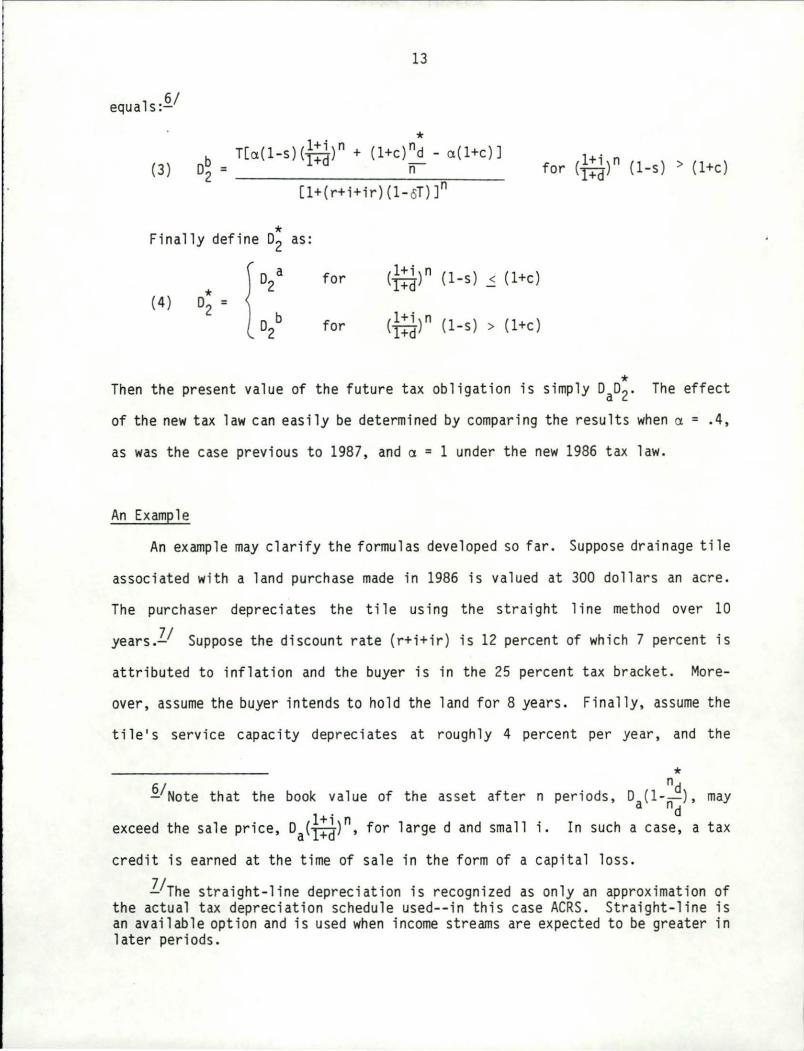
equa 1 s :§_/

* (3)

l+i n n T[a(l-s)(T+d) + (l+c) d - a( l+c)] ob= n 2 ~~~~~~~~~~~~~~-

[ 1 + ( r + i + i r) ( 1 - o T)] n for (f:~ )n (1-s) > (l+c)

Finally define * 02 as:

! o2 a for (l+i)n (1-s) < (l+c)

* l+d -

(4) 02 = D b for (l+i)n (1 -s ) > (l+c) 2 l+d

* Then the present value of the future tax obligation is simply DaD2. The effect

of the new tax law can easily be determined by comparing the results when a = .4,

as was the case previous to 1987, and a= 1 under the new 1986 tax law.

An Example

An example may clarify the formulas developed so far. Suppose drainage tile

associated with a land purchase made in 1986 i s valued at 300 dollars an acr e.

The purchaser depreciates the tile using the straight line method over 10

years.I/ Suppose the discount rate (r+i+ir) is 12 percent of which 7 percent is

attributed to inflation and the buyer is in the 25 percent tax bracket. More­

over, assume the buyer intends to hold the land for 8 years. Finally, assume the

tile's service capacity depreciates at roughly 4 percent per year, and the

* §_/Note that the book value of the asset after n periods, Da(l -~d ) , may

d exceed the sale price, Da(f:~)n, for large d and small i. In such a case, a tax

cred it is earned at the time of sale in the form of a capital loss.

]_/The straight-line depreciation is recognized as only an approximation of the actual tax depreciat ion schedule used--in this case ACRS. Straight-line is an available option and is used when income streams are expected to be greater i n later periods.

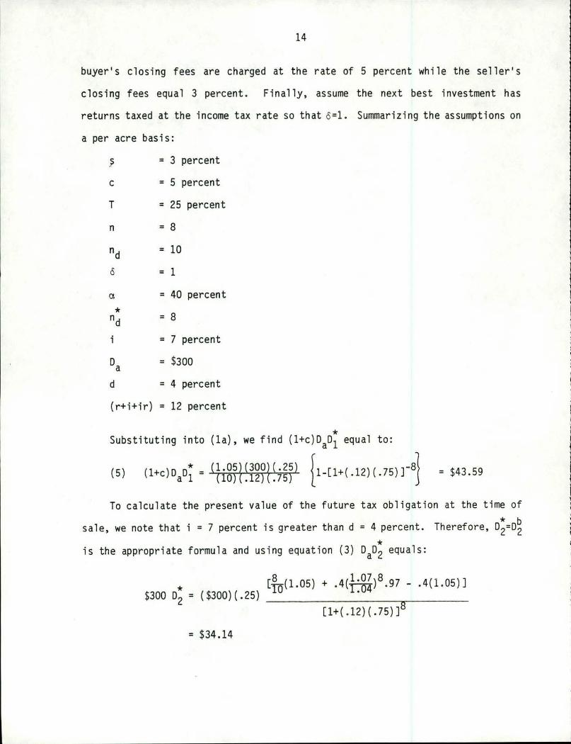
14

buyer• s closing fees are charged at the rate of 5 percent while the seller• s

closing fees equal 3 percent. Finally, assume the next best investment has

returns taxed at the income tax rate so that o=l . Summarizing the assumptions on

a per acre basis:

? = 3 percent

c = 5 percent

T = 25 percent

n = 8

nd = 10

0 = 1

a = 40 percent

* nd = 8

i = 7 percent

oa = $300

d = 4 percent

(r+i+ir) = 12 percent

Substituting into (la) , we find * (l+c)DaDl equal to:

(5) (l+ )o 0• = (I.05!(300!(.25) f 1. [I+(.l2)(. 75 )J-a} c a 1 (IO) .12) . 75) L = $43 .59

To calculate the present value of the future tax obligation at the time of

* b sale, we note that i = 7 percent is greater than d = 4 percent. Therefore, D2=o2 * is the appropriate formula and using equation (3) oao2 equals:

* [fu(l.05) + .4(i:~~) 8 .97 - .4(1.05)J $300 02 = ($300)(.25) - ------ ---- --­

[!+( .12) ( . 75) J8

= $34.14

15

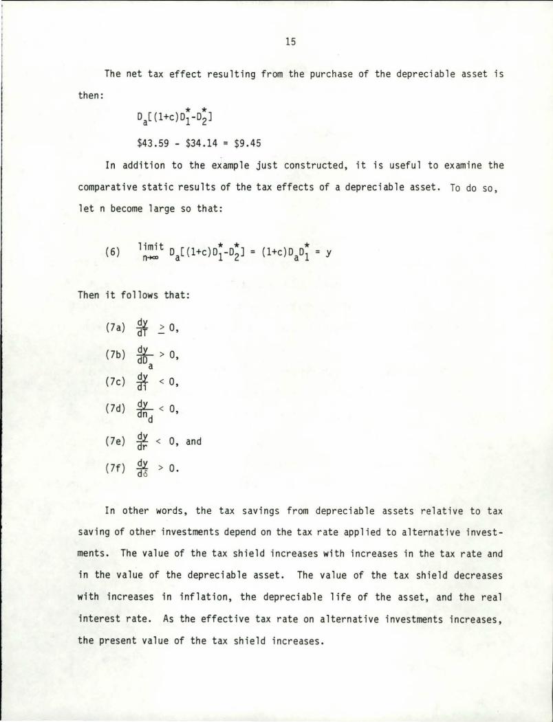
The net tax effect resulting from the purchase of the depreciable asset is

then:

* * Da[(l+c)D1-o2J

$43 . 59 - $34.14 = $9.45

In addition to the example just constructed, it is useful to examine the

comparative static results of the tax effects of a depreciable asset. To do so,

let n become large so that:

(6)

Then it follows that:

(la) El ~ 0, dT

(lb) ~ > 0 dD ' a (le) * < 0,

(ld) ¥n: < 0 ' d

(le) El < dr 0, and

(lf ) El > o. do

In other words, the tax savings from depreciable assets relative to tax

saving of other investments depend on the tax rate applied to alternative invest­

ments. The value of the tax shield increases with increases in the tax rate and

in the value of the depreciable asset. The value of the tax shield decreases

with increases in inflation, the depreciable life of the asset, and the real

interest rate. As the effective tax rate on alternative investments increases,

the present value of the tax shield increases.

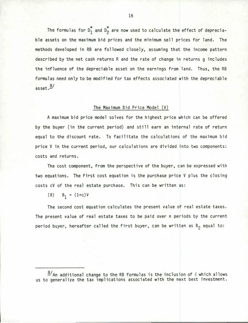
16

* * The formulas for o1 and o2 are now used to calculate the effect of deprecia-

ble assets on the maximum bid prices and the minimum sell prices for land. The

methods developed in RB are followed closely, assuming that the income pattern

described by the net cash returns R and the rate of change in returns g includes

the influence of the depreciable asset on the earnings from land. Thus, the RB

formulas need only to be modified for tax effects associated with the depreciable

asset.~/

The Maximum Bid Price Model (V)

A maximum bid price model solves for the highest price which can be offered

by the buyer (in the current period) and still earn an internal rate of return

equal to the discount rate . To facilitate the calculations of the maximum bid

price V in the current period, our calculations are divided into two components:

costs and returns.

The cost component, from the perspective of the buyer, can be expressed with

two equations. The first cost equation is the purchase price V plus the closing

costs cV of the real estate purchase. This can be written as:

(8) Bl = (l+c)V

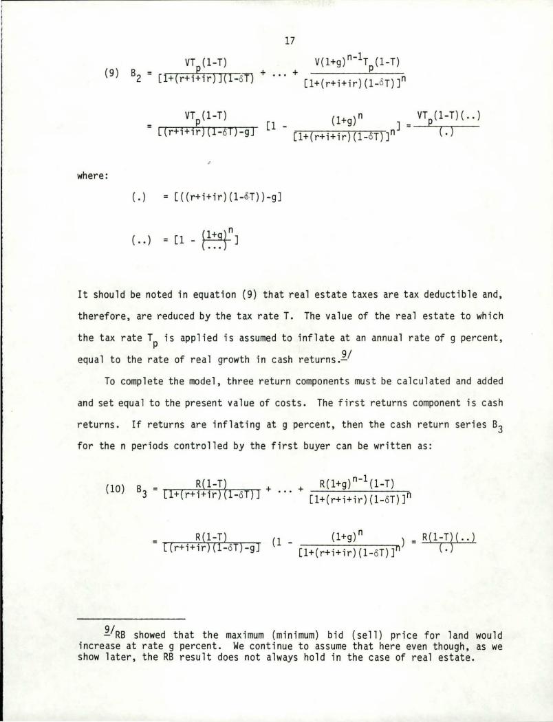
The second cost equation calculates the present value of real estate taxes.

The present value of real estate taxes to be paid over n periods by the current

period buyer, hereafter called the first buyer, can be written as B2 equal to:

§_/An additional change to the RB formulas is the inclus ion of o which allows us to generalize the tax implications associated with the next best investment.

(9)

where:

= VT p (1-T) B2 [l+(r+i+ir)J(l-oll

17

+ ••. + V(l+g)n-lTP(l-T)

[l+(r+i+ir)(l-oT)]n

= VTP(l-T) (l+g)n ] [(r+i+1r)(l-0T)-g] (1 - [l+(r+i+ir)(l-oT)Jn

,·

(.) = [((r+i+ir)(l-©T))-g]

( .. ) = (1 - f:~:~n]

= VT p ( 1-T) ( .. ) ( . )

It should be noted in equation (9) that real estate taxes are tax deductible and,

therefore, are reduced by the tax rate T. The value of the real estate to which

the tax rate Tp is applied is assumed to inflate at an annual rate of g percent,

equal to the rate of real growth in cash returns.~/

To complete the model, three return components must be calculated and added

and set equal to the present value of costs. The first returns component is cash

returns. If returns are inflating at g percent, then the cash return series B3

for the n periods controlled by the first buyer can be written as:

(10) B = R(l-T~ + + R(l+g)n-l(l-T) 3 [l+(r+i+ir) 1-oT)] ··· [l+(r+i+ir)(l-oT)Jn

= R(l-T) [(r+i+ir)(l-oT)-g]

(1 - (1 +g) n ) =

[l+(r+i+ir)(l-oT)Jn

~/RB showed that the maximum (minimum) bid (sell) price for land would increase at rate g percent. We continue to assume that here even though, as we show later, the RB result does not always hold in the case of real estate.

18

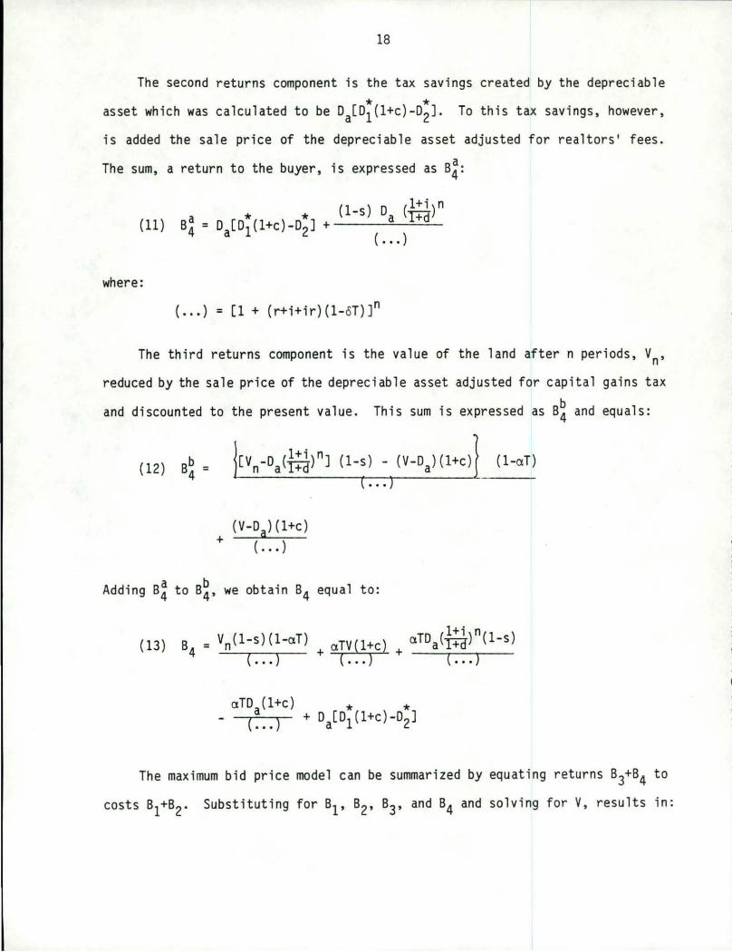
The second returns component is the tax sav i ngs created by the depreciable

* * asset which was calculated to be Da[D1{1+c)-D2J. To this tax savings, however,

is added the sale price of the depreci able asset adjusted for realtors' fees.

The sum, a return to the buyer, is expressed as s;:

where:

( •.• ) = [1 + (r+i+ir)(l-oT)]n

The third returns component is the value of the land after n periods, Vn,

reduced by the sale price of the depreciable asset adjusted for capital gains tax

and discounted to the present value. This sum is expressed as B~ and equals :

(12)

(V-Da)(l+c) + ( ... )

a b Adding B4 to s4• we obtain B4 equal to:

(13) B4

= Vn(l-s)(l-aT) + aTV l+c ( ... )

(1-aT)

aTDa(f!1)n(l-s) + ( ... )

The maximum bid price model can be summarized by equating returns B3+B4 to

costs s1+B2• Substituting for B1, B2, s3, and B4 and solving for V, results in:

19

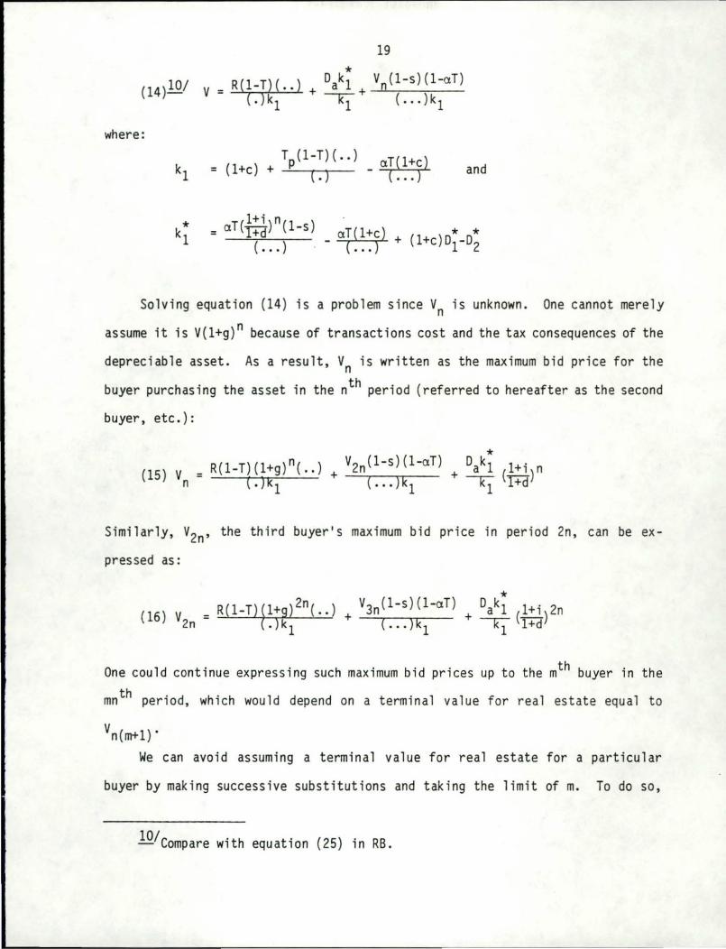
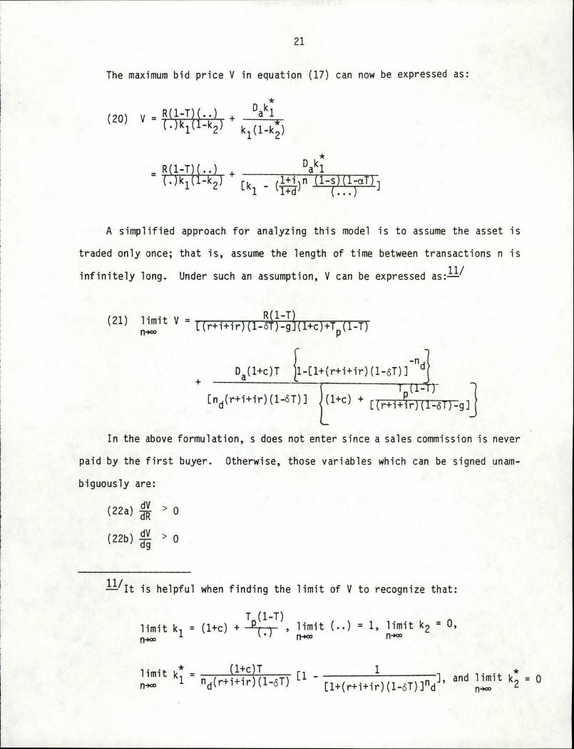
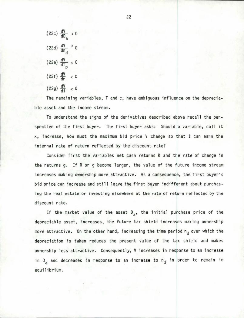
* (14)10/ R{l-T}{ .. } D k Vn{l-s){l-aT)

v = + a 1 + ( . ) kl kl ( ... )kl

where:

kl = Tp(l-T)( .. )

( 1 +c) + ( . ) - ap::}} and

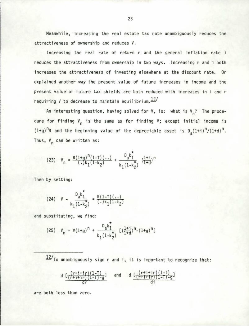
Solving equation (14) is a problem since Vn is unknown. One cannot merely

assume it is V(l+g)n because of transactions cost and the tax consequences of the

depreciable asset. As a result, Vn is written as the maximum bid price for the

buyer purchasing the asset in the nth period (referred to hereafter as the second

buyer, etc.):

Similarly, v2n, the third buyer's maximum bid price in period 2n, can be ex­

pressed as:

One could continue expressing such maximum bid prices up to the mth buyer in the

mnth period, which would depend on a terminal value for real estate equal to

vn(m+l) •

We can avoid assuming a terminal value for real estate for a particular

buyer by making successive substitutions and taking the limit of m. To do so,

lO/compare with equation (25) in RB.

20

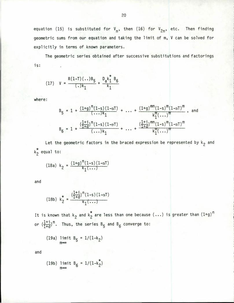
equation (15) is substituted for Vn, then (16) for V2n, etc. Then finding

geometric sums from our equation and taking the limit of m, V can be solved for

explicitly in terms of known parameters .

The geometric series obtained after successive substitutions and factorings

is:

(17)

where:

B5 = 1 + (l+g)n(l-s)(l-aT) + ... + (l+g )mn(l-s )m(l-aT)m and ( ... )kl km ( )m ' 1 ...

l+i n (i:~ ) mn ( l-s ) m ( l-aT )m B = 1 +

(r+a) (1-s) (l-aT) + ... + ( ... )kl kill( ) Ill 6 1 .•.

Let the geometric factors in the braced expression be represented by k2 and

* k2 equal to:

(lBa) k = (l+g)n(l-s )( l-aT) 2 kl ( ... )

and

l+i n * (l+d) (1-s)(l-aT) (18b) k2 = k1( .. . )

It is known that k2 and k; are less than one because ( .. . ) is greater than (l+g )n

or (f:~)n. Thus, the series B5 and B6 converge to:

{19a) limit fll"t<O

B = 5 l/(l-k2)

and

* (19b) limit B6 = l / (l-k2) fll"t<O

21

The maximum bid price V in equation (17) can now be expressed as:

(l+i)n (1-s)(l-af)J 1 +d ( ... )

A simplified approach for analyzing this model is to assume the asset is

traded only once; that is, assume the length of time between transactions n is

infinitely long. Under such an assumption, V can be expressed as:ll/

(21) l" "t V - R(l-Tj imi - [(r+i+ir)(1-8T)-g (l+c)+T (l-T) n-+cio p

Da(l+c)T fl-[l+(r+i+ir)(l-CT)]-nd +

[nd( r+i+ir )( 1-CT) l ( 1 +c) + [ ( r+i+~ r) ~ 1-cTJ-gJJ

In the above formulation, s does not enter since a sales commission is never

paid by the first buyer. Otherwise, those variables which can be signed unam-

bi guous ly are:

dV (22a) dR > 0

(22b) dV > 0 dg

1l11t is helpful when finding the limit of V to recognize that:

T (1-T) limit kl= {l+c) + ~ , limit ( .. ) = 1, limit k2 = 0, n-+cio n-+cio n-+cio

limit k* = {l+c)T (1 - 1 ] and l" "t * n-+cio 1 nd(r+i+ir)(l-oT) [l+(r+i+ir)(l-oT)]nd, n;:1 k2 = 0

22

(22c) ~ dDa

> 0

(22d) dV < 0 dnd

(22e) ~ dTP

< 0

(22f) dV dr < 0

dV (22g) err < 0

The remaining variables, T and c, have ambiguous influence on the deprecia-

ble asset and the income stream.

To understand the signs of the derivatives described above recall the per­

spective of the first buyer. The first buyer asks: Should a variable, call it

x, increase, how must the maximum bid price V change so that I can earn the

internal rate of return reflected by the discount rate?

Consider first the variables net cash returns R and the rate of change in

the returns g. If R or g become larger, the value of the future income stream

increases making ownership more attractive. As a consequence, the first buyer's

bid price can increase and still leave the first buyer indifferent about purchas-

ing the real estate or investing elsewhere at the rate of return reflected by the

discount rate .

If the market value of the asset Da, the initial purchase price of the

depreciable asset, increases, the future tax shield increases making ownership

more attractive. On the other hand, increas i ng the time period nd over which the

depreciat ion is taken reduces the present value of the tax sh ield and makes

ownership less attractive. Consequently, V increases in response to an increase

in Da and decreases in response to an increase to nd in order to remain in

equilibrium.

23

Meanwhile, increasing the real estate tax rate unambiguously reduces the

attractiveness of ownership and reduces V.

Increasing the real rate of return r and the general inflation rate i

reduces the attractiveness from ownership in two ways. Increasing r and i both

increases the attractiveness of investing elsewhere at the discount rate. Or

explained another way the present value of future increases in income and the

present value of future tax shields are both reduced with increases in i and r

requiring V to decrease to maintain equilibrium . .!.£/

An interesting question, having solved for V, is: what is Vn? The proce­

dure for finding Vn is the same as for finding V; except initial income is

(l+g)nR and the beginning value of the depreciable asset is Da(l+i )n/ (l+d )n.

Thus, Vn can be written as:

(23)

Then by setting:

(24)

and substituting, we find:

(l+i)n l+d

lf/To unambiguously sign rand i, it is important to recognize that :

(r+i+irH1-T) J d [(r+1+1r) -1)-g

dr

are both less than zero.

and d [ ( r+ i + i r H 1-T ) ] (r+1+1r) -t)-g

d1

24

Without consideration of a depreciable asset, RB showed capital gains in­

creased at g percent per year. With depreciable assets, the capital gains

earning rate is not just g but also depends on i and d. If {d+g) > i, it can be

easily shown that V changes by a rate less than g.

The formulas derived in the calculation of V will be useful in the calcula­

tion of our second model, the minimum sell pri ce model Vs.

The Minimum Sell Price Model (Vs)

The minimum sell price model calculates the smallest price the seller can

accept and still earn on the real estate an internal rate of return equal to the

discount rate. The minimum sell models differ in significant ways from the

maximum bid models. First, the buying and selling transaction occurs at differ­

ent times for buyers and sellers. A buyer acquires the asset in the current

period and sells it n periods in the future. A seller acquired the asset n0

periods ago and sells it in the current period. This timing difference requires

that taxation associated with the depreciable assets be treated differently

between the maximum bid and minimum sell price models.

For the most part, for depreciable assets placed in service before 1981,

depreciation recapture is ignored if straight-line depreciation has been used.

Under these circumstances, all capital gains are taxed at the capital gains tax

rate aT. In other words, the difference between the depreciable asset's current

market value less its current book value is taxed at the capital gains tax rate.

On the other hand, for depreciable assets placed in service after 1980 and

before 1987, the difference between the asset's current market value and its

current book value is taxed at the income tax rate. If the depreciable asset is

sold for a price exceeding its original purchase price, the difference between

its current market value and the original purchase price adjusted for closing

25

costs is taxed at the capital gains tax rate aT. But, as a result of the new tax

law, beginning in 1987 a = 1.

This difference in the taxation of depreciable assets requires the defini­

tion of a new variable T* equal to:

T if depreciable asset was purchased~ 1981

(26) T* =

aT if depreciable asset was purchased < 1981

Maximum bid and minimum sell price models differ significantly in the treat­

ment of taxes. But in other aspects, they are modeled in similar ways. In the

maximum bid price model, the comparison was between investing at the after-tax

equity at a rate of (r+i+ir)(l-6T) versus the opportunity cost of investing in

land. The present values of the two investments were then set equal to each

other.

The minimum sell price model makes a similar but an alternative comparison .

It compares the present value of after-tax proceeds from the sale of land with

the alternative of keeping the land for an additional n periods. The proceeds

from the land sold are assumed to be invested at the after-tax rate of

(r+i+ir)(l-oT). Equating the present value of the two investments, the mi ni mum

sell price model solves for the selling pri ce which equates the present value of

the two alternatives. We now proceed to construct the minimum sell price model.

Assume the seller has held the land and depreciable asset for n0

periods.

Moreover, let the depreciable asset's current market value be Da, and identify

its original market value n0

periods earlier as Dao · Moreover, the depreciable

asset's current book value value is:

26

The tax obligation created by the sale of the depreciable asset depends on

its purchase date and the size of Da relative to Dao· If Dao is assumed to be

less than Da, then the difference between the depreciable asset's current market

* n value Da and its current book value Da0 (1-~ will create a tax obligation (or

credit) at the tax rate T* which depends on the purchase date. This tax obliga­

tion is calculated as D~ where:

* (28) D3a = T*[ (1-s) D - D (1 - ~) (l+c)]

a ao nd

where: D (1-s) < D (l+c) a ao

Since the tax obligation is owed in the current period, the time of sale, D; is

not discounted. The tax obligation is reduced by closing fees paid to both

purchase and sell the asset.

On the other hand, if Da{l-s) is greater than or equal to Da0

(I+c), then the

seller faces a tax obligation at both the income and capital gains tax rates

depending on the date of purchase. The tax rate on the current market value less

the original purchase price adjusted for closing costs will be taxed at the

capital gains tax rate of .4T if the asset was placed into service before 1987.

The difference between the original purchase price and the current book value n0

periods later adjusted for closing costs is taxed at rate T* which depends on the

purchase date of Dao· This tax obligation where Da(l-s) is greater than Da0

(1+c)

is written as D~:

27

* b n

(29) o3 = [aT Da (l-s) + {l+c) 0ao (~ T* - aT) ] nd

where: D (1-s) > D {l+c) a - ao

* Finally, define o3 as:

* Da for Da(l-s) < Da

0{l+c) 3 ( 30) D3 =

ob 3 for Da (l-s) ~ Oa

0{1+c )

Thus, if the land and attached depreciable asset are sold, a curr ent tax obliga­

* tion on the depreciable asset will be o3 .

On the other hand, the sale price of the depreciable asset, adjusted for

c losing costs, is (1-s)Da. The sale price of the deprec i able asset less tax

obligations can then be defined as:

a * (31) s1 = (1-s)Da - D3

In add i tion, the sale value of the land, a return to the seller, i s calcu-

lated as follows. Let Vs be the sale price of the land plus the deprec i able

asset. Then define Sb as the sale price of the land less taxes wh ich equals:

(32) s~ = [(v5-D.)(l-s)-(l+c)[V

0-Da

0J} (1-aT)

+ [Vo-Dao](l+c)

a b * Final ly, adding s1 to s1, we calculate the net proceeds of t he sale as s1 equal

to:

(33)

28

The alternative to selling the land and depr eciable asset in the current

period is to hold it n periods longer. The value of this alternative is calcu­

lated in much the same way as it was for the maximum bid model . It i ncl udes s3,

the inflating cash returns less the present value of proper ty taxes equal to B2.

It also includes the present value of the tax shield over the remaining deprecia­

ble periods.

* Define ndo as:

* - rd-no (34) ndo -n

* Then the present value of the tax shield is D10 which equals :

( 35 ) D~o = T Dao n d ( r+ i + i r ) ( 1-0 T )

[ 1-[l +( i+r+i r )( l-6T) )-n~o}

The tax obligation assoc i ated with holding the land and depreci able asset

another n periods is calculated next. To do so, consider two cases. First, if

the depreciable's initial purchase price adjusted for clos i ng cost s, Da0

(1+c ) ,

is less than its market value net of closing costs n periods in the future,

Da ( f!~ ) " ( l-s ) , then the difference will be taxed at the tax rate T* whi ch depends

on the depreciable asset's purchase date. This future tax obligation is written

as o~0 which equals:

* n +n (36) D~0 = T*[ (f:J )"Da(l-s ) - Dao (1- d~d 0

){ 1+c) ]

29

On the other hand, if Da(f:d)n(l-s) is greater than Da0(1+c), the seller may

face a future tax obligation at the income and/or capital gains tax rates depend­

ing on when the depreciable(s) are placed in service. This future tax obligation

is written as o~0 which equals:

(37)

* Finally, define 020 as:

(38) for

for

Then the future tax obligation is simply o;0/[l+(r+i+ir)(l-oT)]n.

The second return component resulting from holding the asset an additional

* * n periods rather than selling it equals Da(o10-o20 ); to that amount is added the

sale price of the depreciable adjusted for realtors• fees. Call the result s:0:

The third component of returns resulting from holding land an additional n

periods is the value of the land after n periods, Vn, reduced by the sale of the

depreciable asset adjusted for capital gains recapture tax.

pressed as s~0 and is equal to:

This sum is ex-

(40) B~O = [ [Vn-Da(i:Jl"l

+ [V -D ] (l+c) o ao

(1-s) - [V -D ](l+c)] (1-aT) o ao

30

Adding s:0 to B~o and discounting to the present value, we obtain s40 equal to:

The minimum sell price is now found by equating returns B3+s40 less costs of

* s2 for holding the land plus the depreciable asset to s1, the net returns from

selling the depreciable asset plus land in the current period:

* Substituting for s1, s3, B2, s40 , V, and Vn and solving for Vs results in the

expression:

* R(l-T)( .. )S5 Da S5 (43 ) Vs= (.)k1(1-k

2)(1-s)(l-aT) - (1-s)(l-aT)

1 +i n * * aT Da(J+a) 010-020

+ + ( . . . ) ( 1-a T ) ( ... ) ( 1-s ) ( 1-a T)

aT Da0

(l+c) - ( . . . )(1-s)(l-aT)

aT V0

(l+c) + ( •. . )(1-s){l -aT)

* o3 aT Da aT(l+c)(V0 -Da0 )

+ (1-s)(l-aT) - (1-aT) - (1-s)(l-aT)

where:

and

31

(45)

l+i n( ( 1 +d ) 1-s )( 1-a T) -------] ( ... )

It is helpful at this point to see what comparative static results can be

obtained from the minimum sell price model der i ved above. Before doing so,

however, some simplification is required. The simplication is achieved by allow-

ing n to approach a very large number, suggesting the land is to be traded only

once. Under this assumption, Vs can be expressed as:ll/

( ) = R(l-T)(l+c) 46 1 ~:!t vs [((r+i+ir)(l-of)-g){l+c)+TP(l-T)J(l-s)(l-aT)

-o.r aT( l+c)V0 + aT(l+c)Dao ~] Tp(l-T) - (1-s)(l-aT) (l-s )( l-aT)

(1-s)(l-aT)nd(r+i+ir)(l- T)[l + (r+i+ir)(1-6T)-g]

By using our simplified assumptions and approximations, comparative static re-

sults produce the following unambiguous results:

dV s dV dVS ( 47a) >o ( 47e) cW- > 0 (47i) dR a;- < 0

ao

(47b) dV s

(47f) dV s

< 0 (47j) dVS

- > o dnd aa- > 0 dg

(47c) dV s

(47g) dVS

> 0 dV < 0 as 0

(47d) dV s

0 ( 47h) dV s

< 0 dT < err-p

ll/1t is helpful when finding the limit of Vs to recognize that:

limit s5 = (l+c) n-+oo

limit s; = ________ T __ --=-~~...---n-+oo Tp(l-T)

nd(r+i+ir)(l-oT)[l + (r+i+ir)(l-oT)-g]

and, to simplify matters even more, let:

o* 3 = o3a T* T and = a

(d > i ) ,

(d > i),

32

Interpretations of the derivatives just obtained are now given. Suppose a

variable or parameter other than the minimum sell price Vs i ncreases. Call this

parameter or variable x. Then the derivative answers the question: how will the

minimum sell price adjust so that the same rate of return would be earned from

holding the land another n periods as would be earned from selling it and invest­

ing the proceeds at the rate of return reflected by the discount rate?

To illustrate, suppose expected future returns on real estate increase as a

result of an increase in R or g. Then the minimum sell price would also have to

increase so that returns from the sale of the land would equal the present value

of the returns from n more periods of ownership with increased expected earnings.

Consider now the implication of an increase in the original purchase price

V0

• The first response is to label V0

as a sunk cost and therefore not economic­

ally important. But this would be wrong since increasing V0

reduces capital

gains, thereby increasing the attractiveness of the sell option. Thus, an

increase in V0

does affect the minimum sell price.

Since increasing real estate taxes makes ownership in the future less

attractive, to be indifferent, between ownership in the future or selling now,

the sale price must also decline.

Increasing the original depreciable asset's purchase price, Dao' means that .

there is a larger tax shield for future income. This makes the ownership option

more valuable; so the indifference condition requires that the sale option be

made more attractive--hence the minimum sell price increases. On the other hand,

increasing the tax life of depreciable assets, nd, means that the tax shield will

be available in more distant periods (smaller present value of the t ax shield ) so

that indifference condition requires lowering the minimum sale price.

Increasing realtor fees, increasing s, reduces the actual proceeds received

by the seller. There is, of course, some reduction in the capital gains tax as a

33

result of an increase in s, but this is not nearly as important as the loss in the

proceeds from the sale. Thus, for reasons described earlier, indifference

requires Vs to increase to offset the increase in s.

An increase in the discount rate through an increase in either r, the real

rate of return on an alternative investment, or i, the general inflation rate,

would increase the attractiveness of investing the proceeds from the sale of the

real estate. Thus, equilibrium requires that both an increase in i and r reduces

Increasing the capital gains tax a, particularly from .4 to 1, reduces the

amount of the purchase price returned to the seller. Thus, the minimum sel 1

price must increase with increases in capital gains tax because the seller can

avoid the higher taxes by simply not selling.

Finally, there is one other result not captured by our comparative static

results taken in the limit. What is the optimal value of n? Obviously, as

inflation i or the real interest rate r increases, so does the present value of

the tax shield created by the depreciable asset. As a consequence, more frequent

sales of the asset may be advisable so that the differences between book value

and market value of the depreciable asset do not get too far out of line.

Consider now the current market value of the depreciable asset Da. The ,

higher Da becomes, the greater would be the capital gains tax or income tax paid

* n by the seller . Moreover, since the remaining tax shield is determined by D ~0~ ao n

0

and not by Da, increasing Da does nothing for the seller's future tax shield. As

a consequence:

dVs ( 48) dDa < 0

34

Building Financial Considerations Into Maximum Bid and Minimum Sell Price Models

The financial terms associated with the sale of real estate alter both the

maximum bid and minimum sell prices offered by buyers and accepted by sellers.

In the next section of this paper, we examine the effect on the maximum bid price

when a buyer is financing his real estate purchase with a loan whose interest

rate may differ from that available in the market place or reflected by the

discount rate. Then a similar analysis is completed from the seller's perspec-

tive by asking: What are the effects on the minimum sell price when a seller

provides financing to a buyer at an interest rate which may differ from that

available in the market place or reflected by the discount rate? Consider first,

however, the analysis from the buyer's perspective.

Before proceeding, however, consider the question: Should financial

arrangements be included in the analysis?

In this paper, the financial arrangements are included because their

effects cannot be identified independently of other factors operating in the

model. Consider the dilemma. If the seller offers or the buyer receives a

concessionary interest rate financing, it will require that the seller and buyer

be compensated to determine the new maximum bid or minimum sell price. But the

amount of the compensation will depend on the seller's or buyer's tax position

which depends on what part of the asset is depreciable versus nondepreciable; the

rate of inflation which determines the significance of capital gains income tax

on the sale; and the depreciable asset's book value and the original price of the

depreciable asset which determines what part of the sale price will be paid as

income versus capital gains tax.

The confluence of these factors in the maximum bid and minimum sell models

defies simple subtractions or additions of the effects of financial arrange­

ments. Therefore, this paper argues that they logically belong in the models.

35

The Maximum Bid Price for a Buyer Financed Purchase (V* )

Suppose a buyer is able to finance (1-D) percent of his real estate pur -

chase 's acquisition price at a concessionary interest rater*, wh ich is less than

the discount rate of (r+i+ir). Such a favorable rate may result from a govern­

mental sponsored loan program, such as might be available from the Farmer's Home

Administration, from the transfer of a previous loan contracted by the seller in

periods of lower interest rates, or from a land contract offered by the seller as

an inducement to complete the transaction.

Without financial terms provided the buyer, the maximum bid price was found

to be V. Let the maximum bid price with financial terms provided the buyer be V* .

Moreover, let the amount loaned be (1-D)V* where DV* is the amount of the

purchase price V* paid as a down payment. The after-tax present value of the

loan (1-D)V* repaid at interest rate r* when the market rate of interest is

(r+i+ir) was calculated earlier in RB to be V*f where f equals:li/

(49) f = D + 1-D r* [1-( ... )q-l] + T(l-D ~ r*i···· ) r+ l + l r [ 1 _ ( .. . ) q* -1 ] . )

where:

( ... ) q = [l+(r+i+ir)(l-oT) Jq,

( .. . )q* = (l+r*)q,

( . ) * = [(r+i+ir)(l-oT)-r*], and

( .. .. ) = [ ( ... )q*-1- ( . .. )q-1]

[1- ( .. . )q*-1]

141rn the special case where r* equals (r+i+ir )( l- oT) , f can be expressed as:

qTr* (l-0) f = 1-T + OT + ___ .......___._ __ _. __ _

(l+r*)Q+l(l+r*)

36

An investment of (V*f + cV*) is now compared to which could be invested at

the after-tax rate of return of (r+i+ir)(l- T) the present value of an after-tax

stream of earnings from real estate. The maximum bid price under such a compari-

son can be obtained from the equality below. The opportunity cost is V*f + cV*

because the closing cost is calculated as a percentage of the contract price V*

whi l e the present value of the contract price repaid over q periods at interest

rater* is fV*. One can also show that when r* = (r+i+ir), V = V*.

(50)

where:

* B1 = fV* + cV*, and

l+i n B * _v _..;. n..;....(_1-_s_) ~( 1_-_a T_) + =a T..;....V_*_.__l +,....;;c~ + a T D a ( 1 +d) ( 1-s ) 4- ( .. . ) ( .. . )

* Replacing V in s2 with the right-hand side of (20), and Vn in B4 with the

right-hand side of (23), we solve for V* and obtain the expression below:

(51)

where:

* The Minimum Sell Model with Seller Providing Financing (Vs)

Now consider how the minimum sell price for real estate may be altered when

the seller provides financing. Assume the seller, as a condition of sale, offers

37

a land contract to the buyer for (1-D) percent of the purchase price at an

interest rate r* which may be different than the discount rate (i+r+ir). The

* seller is quite willing to offer the loan of amount (1-D) percent of the sale Vs

at r* less than (greater than) his discount rate of r+i+ir for q periods provided

* Vs is increased (decreased) to offset the loss (gain) in interest income. Of

course, the higher the seller's tax bracket, the more important will be the tax

savings which occurs from having the firm's returns taxed at the capital gains

tax rate (aT) rather than at the income tax rate T.

The 1981 tax law change requires we examine two separate cases. The tax law

change treats differently depreciable assets placed in service before 1981 and

after 1980. Case 1 finds the minimum sell price for a seller financed land plus

depreciable asset sale when the depreciable asset was placed in service before

1981. * Its solution is Vsl where T* = aT. Case 2 finds the min imum sell price

* when the depreciable asset was placed in service after 1980. Its solution is vs 2

for T* = T.

* Case 1: Vsl for T* = aT

Seller financed sales introduce at least one compl icating factor in the

analysis. The complication arises because the purchase price is received in

installments, only part of which could be considered capital gains. Thus, a part

of the principal will be received over time; in addition, part of the capital

gains taxes will also be paid over future time periods. Any interest received by

the seller is, of course, taxed at the seller's ordinary income tax rate. But

the portion of the principal which is taxed depends on when the depreciable asset

was originally purchased.

If the depreciable asset plus land were purchased before 1981, then all the

difference between the current adjusted book value and the depreciable asset's

38

sale price is taxed at the capital gains tax rate of aT. Moreover, if the sale

* price including the depreciable asset is Vsl' then the percentage of the downpay-

ment and principal payments taxed at the capital gains tax rate is equal to :

* n (l+c) (V -0 . ~)

(52) w = 1 - 0 ao nd * vsl(l-s)

To calculate the present value of a seller financed sale, the after-tax

benefits of the loan which is scheduled to be financed for q periods at a

concessionary interest rate r* must be calculated. Define sf0 as the net present

value of after-tax payments P received by the seller for the land sold plus the

downpayment less the sales commission. It can be expressed as :

( 53) a * s10 = (D-s) Vsl (1-waT)

+ ~~~-P~(_l~-a~T_w~)~~~- -~~~P~(_l~-a~T_w~)~~~-+ ••• + (l+r*)q[l+(r+i+ir)(l-OT)] (l+r*)[l+(r+i+ir)(l-oT)]q

P[l-{l+r*)-q]{l-T) + [l+(r+i+ir)(1-oT)J + ••• + P[l-(l+r*)-1](1-T)

[l+(r+i+ir)(l-oT)Jq

Since the downpayment and sales commission were paid initially, the loan pay-

* ment P must be sufficient to retire the amount Vs(l-0) at interest rater* in q

periods. This relationship is expressed below:

( 54) * p 1 {l-D)V = -;:1; [1 - ] s r {l+r*)q

Then, solving for P, obtains:

(55) p = * r*(l-D)V sl

[l-(l+r*)-q]

39

Next we substitute into s~0 for P to obtain an expression for v:1. Simplifying,

after sunrning geometrically, produces the result:l2.1

* (56) s~0 = v:1 f** + [V

0-Dao ~~] (l+c) aT [(D-s) + r*(l(~~i · ···)J/(1-s)

where:

f** = (1-aT)(D-s) + r*(l-D)[l-( ... )q-l] + r*(l-D)T(l-a)( .... ) (r+i+ir)[l-( ..• )q*-l] (.)*

For reasons already given, df**/dr* > 0.

The opportunity cost is again associated with the alternative of holding

real estate another n periods equal to (B3 - B2 + s40 ). This equality is then

expressed as:

And after making the appropriate substitutions, the expression above simplifies

to:

(58)

l+i n aT Da(l+d) (1-s)

+ --...-(-•• - ....... )--* * D10-D20 aT Da

0(1+c )

+ -.-( -.. -. ~) f~*-* - ( .. . ) f **

* aT V

0(l+c)

+ ( ••• )f** [V

0-Dao ~] [(l+c)aT] [D-s + r*(l{~~i · ···)J

(1-s) f**

12_/Note that there is some discrepancy between f** above and f** in RB; even with s and Dao set equal to zero.

40

Case 2: * V for T* = T s2

For depreciable assets placed in service after 1980, a significant tax cost

is introduced into the minimum sell model for a seller financed sale. The

additional cost is: the difference between the depreciable asset's sale price

up to the original purchase ~ price, Dao' less the current depreciated book value

of the depreciable asset taxed at the income tax rate. Moreover, this tax

obligation is due at the time of the sale regardless of the fact that principal

payments for the depreciable asset may not be received until sometime in the

future.

In order to describe this tax obligation due at the time of sale, a new

* variable, Da, is defined equal to:

if (1-D) Da ~ Dao (l+c)

(59) * D = a if (1-D) D a < Dao ( 1 +c)

The tax due at the time of sale is:

* * no (60) T[Da(l-s) - (l+c)Dao (1 - "d)J

Having already paid part of the tax obligation that which remains including any

* created when Da = Dao is repaid over time. It's calculating requires we define

w* equal to:

* * * * (61) w* = [(Vs2-Da)(l-s) (V0

-Da0)(1+c)]/Vs2(1-s)

* V

0{1+c) D {l+c) - D (1-s)

1 - + ao a = * * v52 (1-s) v52 (1-s)

41

The variable w* calculates the percentage of the purchase price required to

pay the tax on the capital gains associated with the land plus any tax due on the

sale of the depreciable asset not already paid.

Having calculated the tax obligation and a new variable w*, we are prepared

* * to find vs2 using much the same procedure used to find Vsi· b First, set s10 equal to:

* b * * n (62) s10 = (0-s)V 2(1-w*aT) - T[O (1-s)-(l+c)O (1-__£_)]

s a ao nd

+ ~~~-P~(_l_-a~T_w~)~~~- -~~~P~(~l~-a~T~w~)~~~-+ ••• + (l+r*)q[l+(r+i+ir)(l-oT)] (l+r*)[l+(r+i+ir)(l-oT)]q

+ P[l-(l+r*)-q](l-T~ + + P[l-(l+r*)-1](1-T) [ 1 + ( r+ i + ; r ) ( 1-o T ) • . . [ 1 + ( r+ i + i r ) ( 1- OT ) ] q

The loan payment P is similar to our earlier expression:

* r*(l-O)V s2 ( 63) p =

Substituting into s~0 for P to obtain an express ion for v:2, after summing

geometrically, produces the result:

(64) Sb = V* f** + Vo(l+c)aT [D + r*{l-D~( . .. . )] 10 s2 (1-s) -s (. *

aT[Da0 (l+c)-D*a(l-s)]( .... ) [D-s + r*(l-0)] {1-s)(.)*

where f** is already defined.

42

The opportunity cost is again associated with the alternative of holding the

real estate another n periods equal to s3 - s2 + s40 • Thus, one can write as an

equality:

(65)

And after making the appropriate substitutions, the expression above simplifies

to :

(66)

l+i n aTDa(l+d) (1-s)

+ ( ••• ) D*10-D* 20

+ __,..,=-=-----==-( ... ) f**

aTDa0(1+c) aTV

0(1+c)

( ... ) f** + ( ... ) f **

+ aT[Da0

(1+c)-D*a(l-s)]( .... ) (l-s)(.)*f** [0-s+r*(l -D) ]

V0 (1+c)aT r*(l-d)~ ... . ) - (1-s)f** [D-s+ (. * J

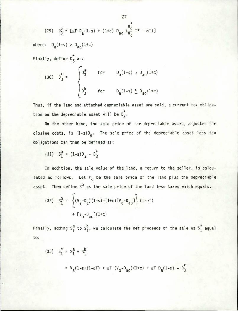
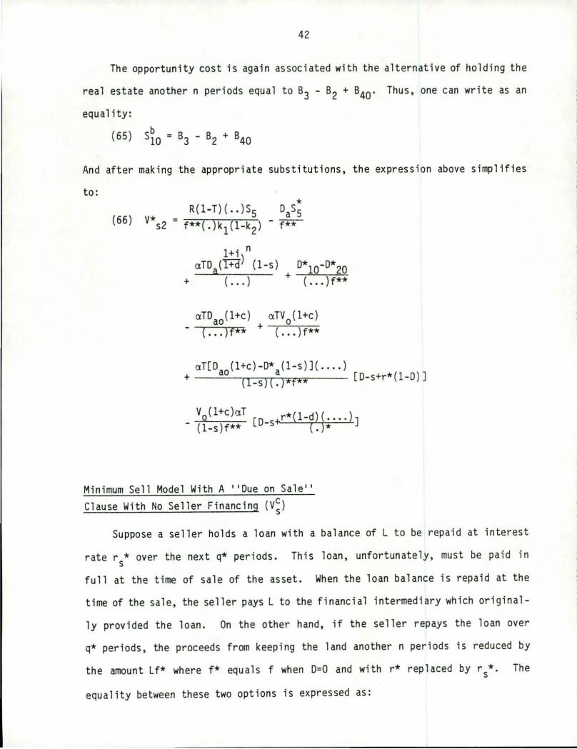
Minimum Sell Model With A ''Due on Sale'' Clause With No Seller Financing (V~)

Suppose a seller holds a loan with a balance of L to be repaid at interest

rate rs* over the next q* periods. This loan, unfortunately, must be paid in

full at the time of sale of the asset. When the loan balance is repaid at the

time of the sale, the seller pays L to the financial intermediary which original­

ly provided the loan. On the other hand, if the seller repays the loan over

q* periods, the proceeds from keeping the land another n periods is reduced by

the amount Lf* where f* equals f when D=O and with r* replaced by r/· The

equality between these two options is expressed as:

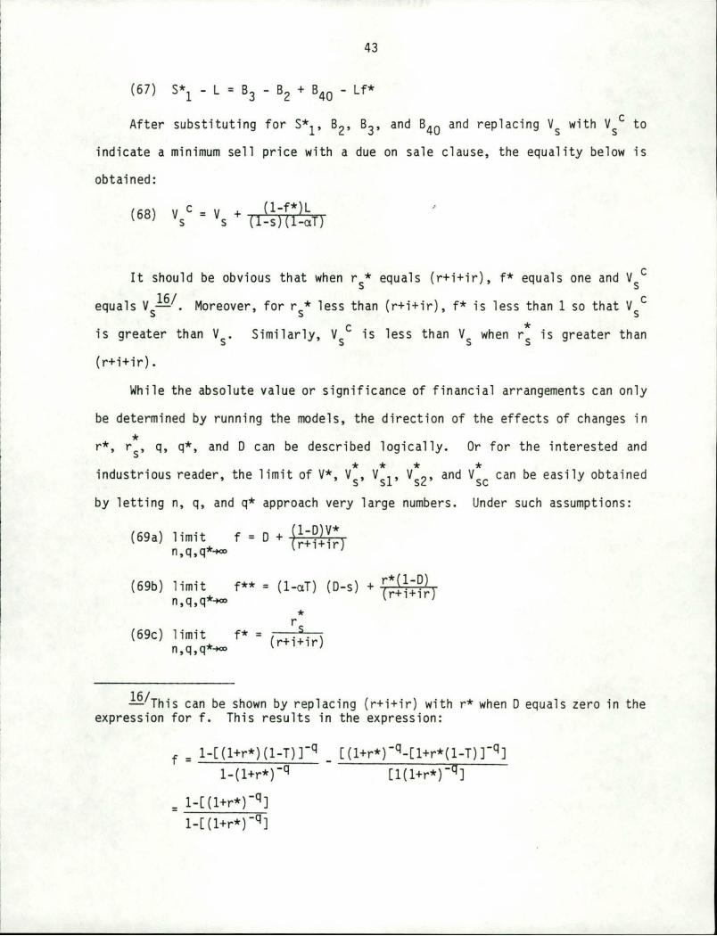
43

(67) S*l - L = 83 - 82 + 840 - Lf*

After substituting for S*1, 82, 83, and 840 and replacing Vs with Vsc to

indicate a minimum sell price with a due on sale clause, the equality below is

obtained:

( ) V c = (1-f*)L 68 s Vs+ (1-s)(l-aT)

It should be obvious that when rs* equals (r+i+ir), f* equals one and Vsc

equals vsJi../. Moreover, for rs* less than (r+i+ir), f* is less than 1 so that Vsc

is greater than Vs. Similarly, Vsc is less than Vs when r: is greater than

(r+i+ir).

While the absolute value or significance of financial arrangements can only

be determined by running the models, the direction of the effects of changes in

* r*, rs, q, q*, and 0 can be described logically. Or for the interested and * * * * industrious reader, the limit of V*, Vs, Vsl' vs2, and Vsc can be easily obtained

by letting n, q, and q* approach very large numbers . Under such assumptions:

( 69a) 1 imit f 0 + 1-0 V* = r+i+ir n,q,q*-+co

(69b) limit f ** = (1-aT) (0-s) + r* 1-0 n,q,q*-+co r+i+ir

* (69c) 1 imit f * =

rs

n,q,q*-+co (r+i+ir)

1.~/This can be shown by replacing (r+i+ir) with r* when O equals zero in the expression for f. This results in the expression :

f = 1-[(l+r*)(l-T)]-q _ 1-(l+r*)-q

= 1-[(l+r*)-q] 1-[(l+r*)-q]

[(l+r*)-q-[l+r*(l-T)]-q] [l(l+r*)-q]

44

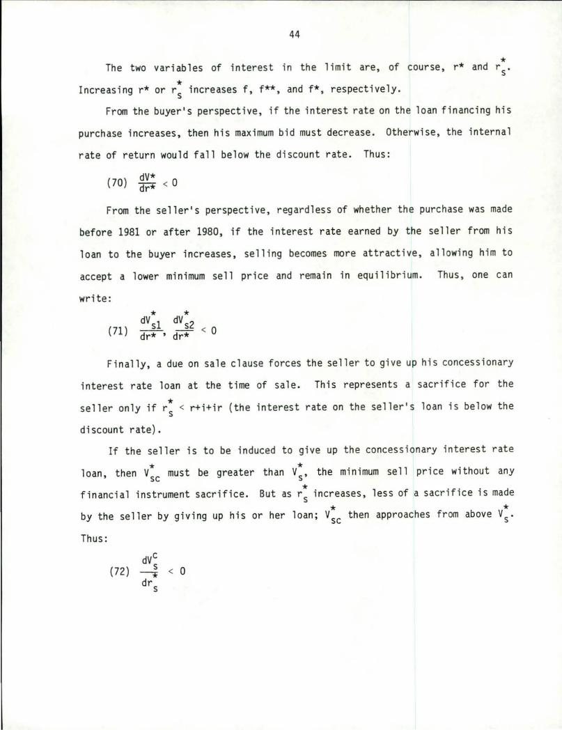
* The two variables of interest in the limit are, of course, r* and rs .

* Increasing r* or rs increases f, f**, and f*, respectively.

From the buyer's perspective, if the interest rate on the loan financing his

purchase increases, then his maximum bid must decrease. Otherwise, the internal

rate of return would fall below the discount rate. Thus:

{70) dV* dr* < O

From the seller's perspective, regardless of whether the purchase was made

before 1981 or after 1980, if the interest rate earned by the seller from his

loan to the buyer increases, selling becomes more attractive, allowing him to

accept a lower minimum sell price and remain in equilibrium. Thus, one can

write :

(71) * * dV sl dV s2

dr* ' dr* < O

Finally, a due on sale clause forces the seller to give up his concessionary

interest rate loan at the time of sale. This represents a sacrifice for the

* seller only if rs < r+i+ir (the interest rate on the seller's loan is below the

discount rate).

If the seller is to be induced to give up the concessionary interest rate

* * loan, then Vsc must be greater than Vs, the minimum sell price without any

* financial instrument sacrifice. But as rs increases, less of a sacrifice is made

* * by the seller by giving up his or her loan; Vsc then approaches from above Vs.

Thus:

(72) < 0

45

Empirical Results

Before reporting empirical results generated by the models, however, we

emphasize the role that maximum bid and minimum sell models play in economic

analysis. Without additional constraints, the models do not necessarily reflect

market prices for an asset; they only reflect break-even conditions for the buyer

or seller. And if the buyer or seller may have opportunities different than

market rates of return, the model results will not reflect market prices.

The model results do though provide useful investment criteri a information.

The break-even price can be compared to the market determined price and the

difference between the two prices is useful investment information. If the

buyer's (seller's) maximum (minimum) bid (sell) price less the market price is

positive (negative), then the net present value association with the purchase

(sale) is positive.

Now we proceed with the description of the model's empirical results . This

description begins with a base case against which the results from changes in the

base model variables are compared.

The base case assumes the market generates the following variables. Let the

real rate of interest be 4 percent. Assume the inflation rate is 4.5 percent and

that the land in question is 100 acres of farmland which in 1981 was valued at

$1,000 per acre. Also assume that attached to the land is a swine finishing

structure constructed in 1981 at a cost of $250,000, or $ 2,500 of building

invested per acre of land. The original purchase price of the real estate in

1981 was therefore $3 ,500 per acre.

The returns from the swine operation on a per acre basis are $250. The land

plus the swine operation are expected to generate returns of $400 per acre the

first year and returns are expected to increase at the rate of 4 percent.

46

The swine finishing structures are expected to be reduced to 5 percent of

their original capacity after 21 years which implies d=.16. For tax purposes,

the structure will be fully depreciated in 5 years. The current market value per

acre of the structure is $ 2 ,500.

The buyer and seller both pay income taxes at the proportional rate of 15

percent, and the transaction is planned to occur before the effective date of the

1986 tax law so that . equals .4. Other tax considerations are property taxes

which are paid at the rate of 2.5 percent and the opportunity tax weight coeffi­

cient is cS= l.

Transactions costs include 5 percent realtor fees paid by the seller and 2.5

percent closing fees paid by the buyer. Fina ncial arrangements include a 7.5

percent note held by the seller, with $2,500 per acre outstanding, with 20 years

remaining until maturity. The buyer, on the other hand, can negotiate a FmHA

loan at 5 percent for 20 years to cover 75 percent of the purchase . Finally, if

the purchase is completed, the buyer is expected to hold the land and attached

buildings for 20 years.

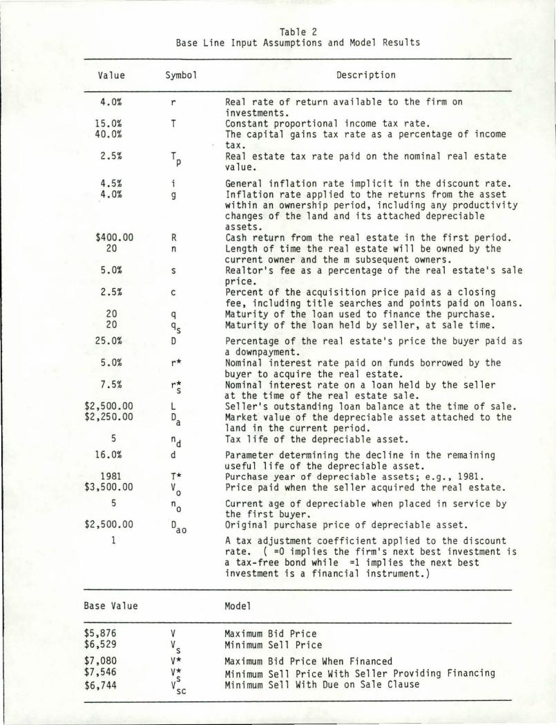
A summary of these base line data assumptions used in the example is pro­

vided in Table 2.

The model results from the base line data are also described in Table 2.

Ignoring financial considerations, the maximum bid price is $5,694.22 . The

minimum sell price is $6,569 .87. Without financial considerations, the buyer and

seller would never transact with each other since the buyer's maximum bid price

is less than the seller's minimum sell price. This, of course, implies the

seller could not sell to himself or herself and make money on the transaction.

Value

4.0%

15.0% 40.0%

2.5%

4.5% 4.0%

$400.00 20

5.0%

2.5%

20 20

25.0%

5.0%

7.5%

$2,500.00 $2,250.00

5

16.0%

1981 $3,500.00

5

$2,500.00 1

Base Value

$5,876 $6,529

$7,080 $7,546 $6,744

Table 2 Base Line Input Assumptions and Model Results

Symbol

r

T

Tp

g

R n

s

c

q qs D

r*

r* s

L Da

nd d

T* Vo no

0ao

v vs V* V* vs

SC

Description

Real rate of return available to the firm on investments. Constant proportional income tax rate. The capital gains t ax rate as a percentage of income tax. Real estate tax rate paid on the nominal real estate value.

General inflation rate implic i t in the discount rate. Inflation rate applied to the returns from the asset within an ownership period, including any productivity changes of the land and its attached depreciable assets. Cash return from the real estate in the f irst period. Length of time the real estate will be owned by the current owner and the m subsequent owners. Realtor's fee as a percentage of the real estate ' s sale price. Percent of the acquisition price paid as a closing fee, including title searches and points paid on loans. Maturity of the loan used to f i nance the purchase. Maturity of the loan held by seller, at sale time. Percentage of the real estate's price the buyer pa i d as a downpayment. Nominal interest rate paid on funds borrowed by the buyer to acquire the real estate. Nominal interest rate on a loan held by the seller at the time of the real estate sale. Seller's outstanding loan balance at the time of sale. Market value of the depreciable asset attached to the land in the current period. Tax life of the depreciable asset. Parameter determining the decline in the remaining useful life of the depreciable asset. Purchase year of depreciable assets; e.g., 1981. Price paid when the seller acquired the real estate . Current age of depreciable when placed in service by the first buyer. Original purchase price of depreciable as set. A tax adjustment coeffic ient appl i ed to the discount rate. ( =O implies the firm's next best investment is a tax-free bond while =l implies the next best investment is a financ ial instrument.)

Model

Maximum Bid Price Minimum Sell Price

Maximum Bid Price When Financed Minimum Sell Price With Seller Providing Financing Minimum Sell With Due on Sale Clause

48

On the other hand, if the buyer's purchase is partially financed at 5

percent, the maximum bid price increases to $6,889.34 exceeding the minimum sell

price without financial consideration and also greater than the minimum sell

price with a due on sale clause. As one would expect, however, if the seller must

provide the 5 percent financing of the buyer, the minimum sell price increases to

$7,568.70 and no sale is possible.

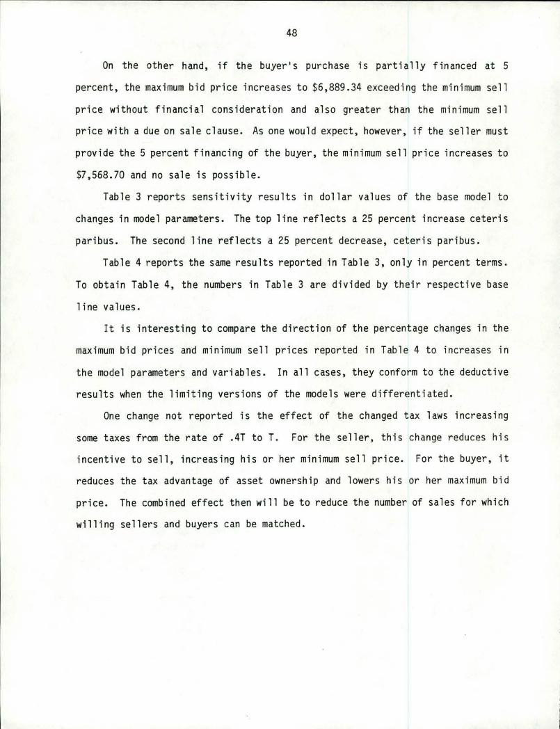
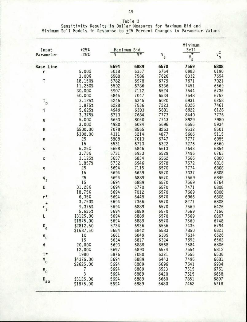
Table 3 reports sensitivity results in dollar values of the base model to

changes in model parameters. The top line reflects a 25 percent increase ceteris

paribus. The second line reflects a 25 percent decrease, ceteris paribus.

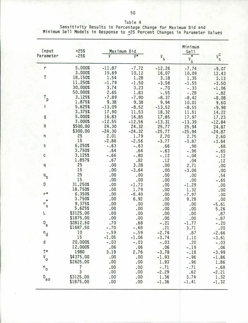
Table 4 reports the same results reported in Table 3, only in percent terms.

To obtain Table 4, the numbers in Table 3 are divided by their respective base

line values.

It is interesting to compare the direction of the percentage changes in the

maximum bid prices and minimum sell prices reported in Table 4 to increases in

the model parameters and variables. In all cases, they conform to the deductive

results when the limiting versions of the models were differentiated.

One change not reported is the effect of the changed tax laws increasing

some taxes from the rate of .4T to T. For the seller, this change reduces his

incentive to sell, increasing his or her minimum sell price. For the buyer, it

reduces the tax advantage of asset ownership and lowers his or her maximum bid

price. The combined effect then will be to reduce the number of sales for which

willing sellers and buyers can be matched.

49

Table 3 Sensitivity Results in Dollar Measures for Maximum Bid and

Minimum Sell Models in Response to ~25 Percent Changes in Parameter Values

Mini mum Input +25% Maximum Bid Sell

Ve Parameter -25% v V* vs * vs s

Base line 5694 6889 6570 7569 6808 r 5.00% 5018 6357 5764 6983 6190

3.00% 6588 7586 7626 8332 7654 T 18.150% 5782 6978 6779 7671 7021

11. 250% 5592 6786 6336 7451 6569 30.00% 5907 7112 6524 7544 6736 50.00% 5845 7047 6534 7548 6752

Tp 3.125% 5245 6345 6020 6931 6258 1.875% 6228 7536 7223 8326 7461 5.625% 4949 6303 5681 6922 6128 3.375% 6713 7684 7773 8440 7776

g 5.00% 6653 8050 7743 8929 7980 3.00% 4980 6024 5696 6555 5934

R $500.00 7078 8565 8263 9532 8501 $300.00 4311 5214 4877 5606 5115

n 25 5808 7013 6747 7777 6985 15 5531 6713 6322 7276 6560

s 6.25% 5658 6846 6613 7643 6854 3.75% 5731 6933 6529 7496 6763

c 3.125% 5657 6834 6562 7566 6800 1.857% 5732 6946 6578 7572 6816

q 25 5694 7115 6570 7774 6808 15 5694 6639 6570 7337 6808

qs 25 5694 6889 6570 7569 6845 15 5694 6889 6570 7569 6764

D 31. 25% 5694 6770 6570 7471 6808 18.75% 5694 7012 6570 7669 6808

r* 6.35% 5694 6448 6570 6966 6808 * 3.750% 5694 7366 6570 8271 6808

r 9.375% 5694 6889 6570 7569 6426 s 5.625% 5694 6889 6570 7569 7166 L $3125.00 5694 6889 6570 7569 6867

$1875.00 5694 6889 6570 7569 6748 Da $2812.50 5734 6936 6556 7435 6794

$1687.50 5654 6842 6583 7850 6821 nd 10 5661 6849 6389 7634 6626

15 5634 6817 6324 7652 6562 d 20.00% 5693 6888 6568 7584 6806

12. 00% 5697 6893 6574 7554 6812 T* 1980 5876 7080 6321 7555 6536 Vo $4375. 00 5694 6889 6443 7496 6681

$2625.00 5694 6889 6696 7641 6934 no 7 5694 6889 6523 7515 6761

3 5694 6889 6420 7615 6658 Dao $3125.00 5694 6889 6660 7851 6897

$1875.00 5694 6889 6480 7462 6718

50

Table 4 Sensi t ivity Results in Percentage Change for Maximum Bid and

Minimum Sell Models in Response to ~25 Percent Changes in Parameter Values

Minimum Input +25% Ma xi mum Bid Sell

Parameter -25% v V* vs * Ve vs s

r 5.000% -11.87 -7.72 -12.26 -7.74 - 9. 07 3.000% 15.69 10. 12 16 . 07 10. 09 12 .43

T 18 .150% 1. 54 1.28 3. 18 1.35 3.13 11. 250% -1. 79 -1.50 -3. 56 -1. 55 - 3. 50 30.000% 3.74 3.23 -.70 -.33 -1.06 50.000% 2.65 1.83 -.55 -.28 -. 82

Tp 3.125% -7.89 - 7. 90 -8.37 -8.42 -8.08 1.875% 9. 38 9.38 9.94 10.01 9.60

; 5.625% -13.09 - 8.52 -13.52 -8 . 55 -9 .98 3.375% 17.90 11.53 18 . 32 11.51 14 . 22

g 5.000% 16 .83 16 .85 17.85 17 . 97 17.23 3.000% -12.55 - 12.56 -13.31 -13.39 -12.84

R $500.00 24.30 24.32 25. 77 25.94 24 .87 $300.00 -24.30 -24.32 -25.77 -25.94 -24.87

n 25 2. 01 1. 79 2.70 2.75 2. 60 15 -2.86 -2.56 -3 . 77 -3.87 -3.64

s 6.250% - .63 -.63 .66 .98 .68 3.750% .64 . 64 -.63 -.96 -. 65

c 3.125% -.66 -.80 -.12 -.04 - .12 1.857% . 67 .82 .12 . 04 .12

q 25 .00 3. 28 .00 2. 71 . 00 15 .00 -3.64 .00 -3.06 . 00

qs 25 .00 . 00 .00 . 00 . 54 15 .00 .00 .00 .00 -. 65

D 31. 250% .00 -1. 73 .00 -1.29 .00 18.750% .00 1.79 . 00 1.32 .00

r* 6. 350% . 00 -6.40 .00 -7.97 . 00

* 3. 750% .00 6.92 .00 9. 28 .00

r 9.375% . 00 .00 .00 .00 - 5. 61 s 5.625% . 00 .00 .00 .00 5.26 L $3125 .00 .00 .00 . 00 .00 .87

$1875.00 . 00 .00 .00 .00 -. 87 Da $2812.50 • 70 .68 - . 21 -1. 77 - .20

$1687.50 -.70 -.68 . 21 3. 71 . 20 nd 10 - . 59 -.59 -2.76 .87 - 2. 66

15 -1.05 - 1.06 - 3. 74 1.10 -3. 61 d 20.000% -.03 -.03 - .03 .20 -. 03

12.000% .06 . 06 .06 -.19 . 06 T* 1980 3.19 2. 76 - 3.78 -.18 - 3. 99 Vo $4375 . 00 . 00 .00 - 1.93 -.96 -1.86

$2625.00 . 00 .00 1.93 .96 1.86 n 7 .00 .00 - • 71 - • 71 -.68 0 3 .00 .00 -2.29 .62 -2.21 0ao $3125.00 .00 .00 1.36 3.74 1.32

$1875 .00 . 00 .00 -1.36 -1. 41 -1.32

51

Epilogue

Real estate buy and sell decisions can be very complicated to calculate.

They are complicated by differential tax effects depending on cut-off dates on

tax rate changes, property taxes, and tax shields created by depreciation and

capital gains. They are further complicated by special financial terms which

affect buyers and sellers differently. As more realism is included, maximum bid

and minimum sell models become more complex.

This paper's approach has been to build comprehensive bid and sell models

piece by piece and then combine the results. Approached in that manner, the

process can be understood and analyzed.

Models of the type constructed in this paper are intended to be decision

aids--and not the decision making model. They cannot be the only basis for

decisions because no one can supply the perfectly accurate data they require for

perfect estimates of maximum bid and minimum sell prices. At best they can be

estimated under alternative scenarios to find the range of possible outcomes.

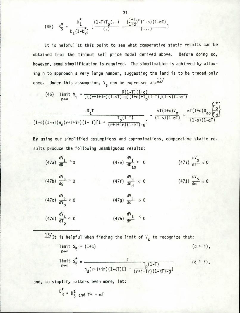
The usefulness of present value models as an analytic tool has been fre­

quently overlooked. One possible explanation for their lack of analytic use is

that they can quickly become complicated. To be analytically useful present

value models must often be simplified. The models in this paper were simplified

by increasing the holding period n to a very large number. Then once simplified

the models were differentiated to predict directional response to variable and

parameter changes. In all cases, the analytic predictions were consistent with

the direction of nominal changes obtained using the more complicated models.

We reconunend that the use of present value models as an analytic as well as

empirical tool be increased. This, of course, will require that present value

models be constructed using geometric series rather than simply expressed as

numerical sums. There is a saving, however, from using geometric series: future

52

cash flow streams can be expressed in terms of geometric means--variables more

likely to be estimable than mn individual data points. Hopefully, the models and

approach followed in this paper have provided a useful illustration of how useful

analytic and empirical present value models can be constructed and used.

53

References

Aplin, R.D., G.L. Casler, and C.P. Francis. Capital Investment Analysis Using Discounted Cash Flows. 2nd Edition. Columbus, Ohio: Grid. 1977.

Baker, T.G. ''An Income Capitalization Model of Land Value with Income Tax Considerations.' 1 Journal Paper No. 47907. Purdue Agricultural Experiment

Station. June 1981.

Bierman, H., Jr. and S. Smidt. The Capital Budgeting Decision. 4th Edition. New York : Macmillan. 1971.

Brealey, R. and S. Myer. Principles of Corporate Finance. New York: McGraw­Hi 11. 1981.

Canada, J.R. and J .A. White, Jr. Capital Investment Decision Analysis for Man­agement and Engineering. Englewood Cliffs, N.J . : Prentice-Hall. 1980.

Lee, W.F. and N. Rask. 1 'Inflation and Crop Profitability: How Much Can Farm-ers Pay for Land?' 1 American Journal of Agricultural Economics 58(1976):984-990.

Robison, L.J. and W.G. Burghardt. 1 'Five Principles for Building Present Value Models and Their Application to Maximum {Minimum) Bid (Sell) Price Models for Land.' 1 Michigan Agricultural Experiment Station Journal Article No. 11051.