+ All Categories
Home > Documents > RIETI BBL Seminar Handout · richard baldwin professor of international economics ... 1962 1965...

RIETI BBL Seminar Handout · richard baldwin professor of international economics ... 1962 1965...

Date post: 13-Dec-2018
Category:
Upload: lamxuyen
View: 215 times
Download: 0 times
Share this document with a friend
38
RIETI BBL Seminar Handout December 11, 2018 Speaker: Richard Baldwin https://www.rieti.go.jp/jp/index.html Research Institute of Economy, Trade and Industry (RIETI) “GVC Journeys When National and Territorial Comparative Advantage Differ
Transcript

RIETI BBL Seminar Handout

December 11, 2018Speaker: Richard Baldwin

https://www.rieti.go.jp/jp/index.html

Research Institute of Economy, Trade and Industry (RIETI)

“GVC Journeys When National and Territorial Comparative Advantage Differ”

RICHARD BALDWINP RO F E S SO R   O F   I N T E RNAT I ONA L   E CONOM I C STHE GRADUATE INSTITUTE I GENEVA

GVC Journeysby Richard Baldwin & Toshihiro Okubo

Background question:

Was comparative advantage denationalised?

#1. EMs lowered tariffs a lot

AEs much less

3

South Asia

Sub-Saharan Africa

Middle East & North Africa

East Asia

US, Japan & EU0

5

10

15

20

25

30

35

40

45

50

1988

1989

1990

1991

1992

1993

1994

1995

1996

1997

1998

1999

2000

2001

2002

2003

2004

2005

2006

2007

2008

Applied tariffs (%)

#2. Shocking Share Shift in Manufacturing.

World shares: ‐ 7 ‘losers’‐ 7 ‘risers’‐ RoW = little change.

1990, G7

65%

3%

6 risers,

5%

RoW

47%

China, 18%

9%

0%

10%

20%

30%

40%

50%

60%

70%

80%

1970

1975

1980

1985

1990

1995

2000

2005

2010

Wor

ld m

anuf

actu

ring

shar

e

Source: unstats.un.org; 6 risers = Korea, India, Indonesia, Thailand, Turkey, Poland

Germany-France

US-Mexico

Germany-PolandUS-

Mexico

Japan-Thailand

0%

10%

20%

30%

40%

50%

60%

70%

80%

1962

1965

1968

1971

1974

1977

1980

1983

1986

1989

1992

1995

1998

2001

2004

2007

2010

Intraindustry trade indices#3. Two‐way trade in similar goods goes North‐South, too

5

1990

Germany-France

US-Mexico

Germany-PolandUS-

Mexico

Japan-Thailand

0%

10%

20%

30%

40%

50%

60%

70%

80%

1962

1965

1968

1971

1974

1977

1980

1983

1986

1989

1992

1995

1998

2001

2004

2007

2010

Intraindustry trade indices#4. Two‐way trade in similar goods goes North‐South, too

6

1990

#5. Parts and components flow “wrong way”?

What explains this?

1. Old Globalisation (1st unbundling): Lower barriers allow nations to exploit existing comparative advantage. (Trade‐led globalisation)

2. New Globalisation (2nd unbundling): Better ICT allows North‐>South flows of firm‐specific knowhow that changes existing comparative advantages. (Knowledge‐led globalisation)

8

Weak direct evidence of knowledge flows

9

‐5

5

15

25

35

45

55

65

75

85

95

‐5

0

5

10

15

20

25

1980

1982

1984

1986

1988

1990

1992

1994

1996

1998

2000

2002

2004

2006

2008

2010

2012

2014

2016

Net receipts for IP (billion US$) 

Germany

Japan

US (rightscale)

‐30

‐25

‐20

‐15

‐10

‐5

0

‐7

‐6

‐5

‐4

‐3

‐2

‐1

0

1980

1982

1984

1986

1988

1990

1992

1994

1996

1998

2000

2002

2004

2006

2008

2010

2012

2014

2016

Net receipts for IP (billion US$) 

Korea, Rep.

Mexico

Thailand

China (right scale)

Actual question addressed in this paper: Can we identify GVC “paradigms”?

• Like “Inward Oriented” vs “Export Oriented” development paradigms of yesteryear?

• e.g. Thailand focused on autos; Philippines much broader; Costa Rica focused on services, etc.

• Can we classify the “GVC Industrialisation Journeys” into helpful categories?

Trade in parts vs final goods

The necessary suspense of disbelief:• Assume exporting parts from South to North reflects 

North‐tech + South‐wages  (the tech is in the parts)• Export of final goods less so (assembly activity is 

simpler and ubiquitous before 2nd unbundling)But may be interesting even without suspended disbelief

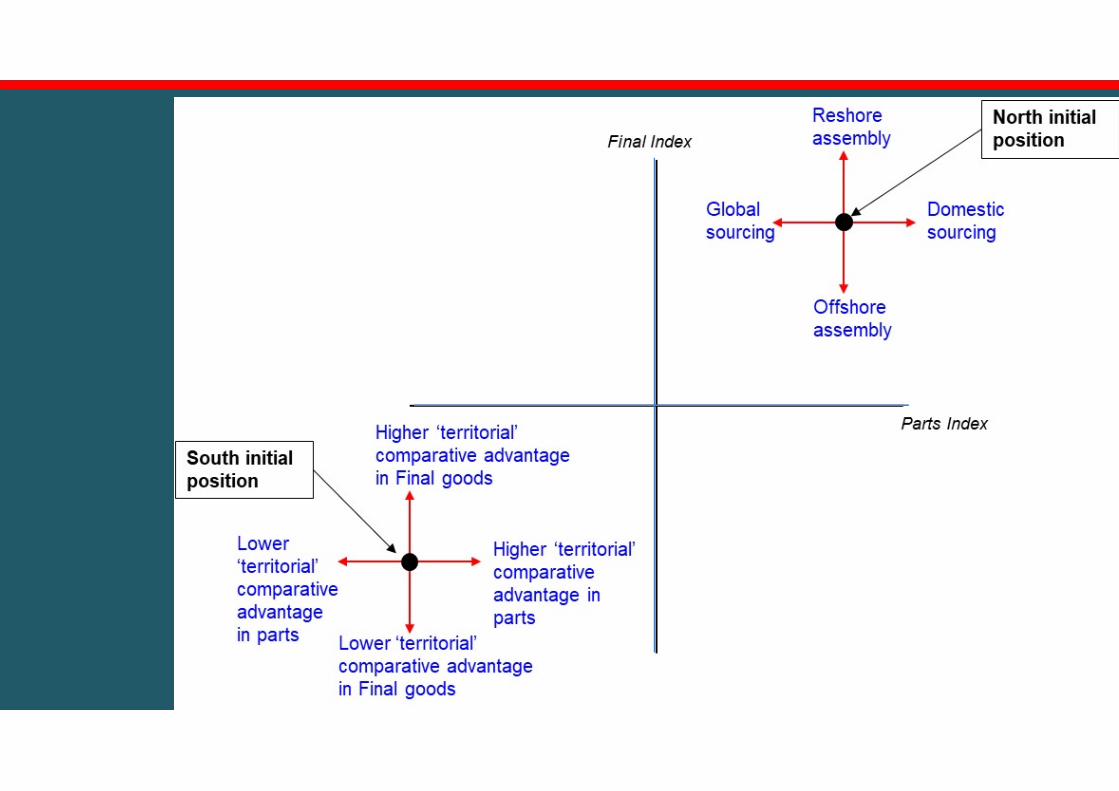
The GVC Journey diagram

‐ 1. Empirical Comparative Advantage (ECA) index

‐ For country ‘c’ in sector ‘i’ and k=parts, or goods‐ Measures “Territorial Comparative Advantage” (Comp.Adv. when 

sources of comp.adv. cross borders within int’l supply chains)

‐ From ‐1 (comp.disadv) to 1 (comp.adv.)

GVC Journey diagram Goods ECA

index

Parts ECA Index

GVC journey diagram

(+,‐)Emp.Comp.Adv. in parts, not goods

(+,‐)Emp.Comp.Adv. in parts, not goods

(‐,‐)Emp.Comp.Disdv. in 

parts & goods(typical EM pre‐1990)

(‐,‐)Emp.Comp.Disdv. in 

parts & goods(typical EM pre‐1990)

(‐,+)Emp.Comp.Adv. in goods, not parts

(‐,+)Emp.Comp.Adv. in goods, not parts

(+,+)Emp.Comp.Adv. in parts & goods(typical G7?)

(+,+)Emp.Comp.Adv. in parts & goods(typical G7?)

Example of paradigms

ECA goods

ECA parts

Pure import substitution

Example of paradigms

ECA goods

ECA parts

Successful export‐led industrialisation

Example of paradigms

ECA goods

ECA parts

Assembly export‐platform

Germany’s GVC Journey0.6

0.4

Transportation equip

Other machinery

Electrical & Optical 

Germany’s GVC Journey ‐ STYLISEDTransp.

Global sourcing boosts comp.adv. 

in final

OtherMachOffshoring production

Electrical & Optical Offshoring production

US’s GVC Journey

‐0.1

0.2

Transp.Eq

Other machineryElectrical & Optical 

‐0.4

Japan’s GVC Journey1.0

1.0

Transp.EqOther machinery

Electrical & Optical 

0.0

China’s GVC Journey0.8

0.4

Transp.EqOther machinery

Electrical & Optical 

‐0.4

Mexico

Mexico

EMs lowered tariffs; AEs much less

28

0

10

20

30

40

50

60

1981

1983

1985

1987

1989

1991

1993

1995

1997

1999

2001

2003

2005

2007

2009

ThailandMalaysiaIndonesiaTaiwan,ChinaChinaPhilippinesKorea Rep.

1990

Spider: Basic assumptions• Perfect competition, constant return, 2 regions.• All final consumption in North.

– Shipping costs of final good t = traditional trade costs

• Coordination cost:– Per-unit costs is tθ(y) paid if part not produced in region of assembly.

= efficiency loss due to spatial separation.

29

Comparative advantagePARTS: Parts are indexed by type y ε Y• Unit production cost are:

– b(y) in S– normalised to 1 in N.

• S has comp.adv. in parts b(y)<1

ASSEMBLY: Assembly of parts costs: • aN in N • aS in S.

– S has comp.adv. in assemble iff aS<aN.

30

Intermed results: Spider

bbN = 1 + θ

bS = 1 - θ

N

S

NS

b

b

1

Part’s relative cost in S

Part’s coordination cost

Each part is a point in b, space.Part’s relative cost in S

Threshold part; assembly in S

Threshold part; assembly in N

Spider

32

bbN = 1 + θ

bS = 1 - θ

N

S

NS

b

b

1

Part’s relative cost in S

Part’s Offshoring cost

3 sets of parts, N, NS, S N: always cheapest in N S: always cheapest in S. NS: cheapest to co-locate

with assembly.

Cost minimisation

• Given sets N, S and NS chosen to min costs for given t• Assembly in S iff

• is greater than

33

dyyytybdyyayyN

SNSN

)()()()(1

dyyybdyyyttayyS

NSSN

)()()()(1

(1)

.

Offshore ‘overshooting’ & ‘reshoring’• Easy results:.

– Shift in assembly leads to ‘too much’ parts overshooting (compared to costless trade case) likely to occur.

– Lowering ‘t’ reverses this ‘reshoring’.

34

bbN = 1 + θ

bS = 1 - θ

N

S

NS

b

b

1

Simple example• Focus on comparative advantage;

- Assume all coordination costs,’s, equal for all parts, so horizontal axis now “t” , not theta

• Start with assembly in North; assume aS<aN.

35

2/)( bbtA 2/)( bbtR

2/)( bbtA 2/)( bbtR

Result: Offshoring “overshooting” of parts

Assembly in S tAssembly in N

b = 1

N

S

NS

Production technology and distribution of comparative advantage

36

Asymmetric parts production and exports with knowledge-led globalisation

37


Recommended