Katerina Simons Economist, Federal Reserve Bank of Boston. The author is grateful to Rich- ard Kopcke and Peter Fortune for help- ful comments and to Jay Seideman for excellent research assistance. Risk-Adjusted Performance of Mutual Funds T he number of mutual funds has grown dramatically in recent years. The Financial Research Corporation data base, the source of data for this article, lists 7,734 distinct mutual fund portfolios. Mutual funds are now the preferred way for individual investors and many institutions to participate in the capital markets, and their popu- larity has increased demand for evaluations of fund performance. Busi- ness Week, Barron’s, Forbes, Money, and many other business publications rank mutual funds according to their performance. Information services, such as Morningstar and Lipper Analytical Services, exist specifically for this purpose. There is no general agreement, however, about how best to measure and compare fund performance and on what information funds should disclose to investors. The two major issues that need to be addressed in any performance ranking are how to choose an appropriate benchmark for comparison and how to adjust a fund’s return for risk. In March 1995, the Securities and Exchange Commission (SEC) issued a Request for Comments on “Im- proving Descriptions of Risk by Mutual Funds and Other Investment Companies.” The request generated a lot of interest, with 3,600 comment letters from investors. However, no consensus has emerged and the SEC has declined for now to mandate a specific risk measure. Risk and performance measurement is an active area for academic research and continues to be of vital interest to investors who need to make informed decisions and to mutual fund managers whose compen- sation is tied to fund performance. This article describes a number of performance measures. Their common feature is that they all measure funds’ returns relative to risk. However, they differ in how they define and measure risk and, consequently, in how they define risk-adjusted performance. The article also compares rankings of a large sample of funds using two popular measures. It finds a surprisingly good agree- ment between the two measures for both stock and bond funds during the three-year period between 1995 and 1997.
Transcript
Katerina Simons
Economist, Federal Reserve Bank ofBoston. The author is grateful to Rich-ard Kopcke and Peter Fortune for help-ful comments and to Jay Seideman forexcellent research assistance.
Risk-AdjustedPerformance ofMutual Funds
The number of mutual funds has grown dramatically in recentyears. The Financial Research Corporation data base, the source ofdata for this article, lists 7,734 distinct mutual fund portfolios.
Mutual funds are now the preferred way for individual investors andmany institutions to participate in the capital markets, and their popu-larity has increased demand for evaluations of fund performance. Busi-ness Week, Barron’s, Forbes, Money, and many other business publicationsrank mutual funds according to their performance. Information services,such as Morningstar and Lipper Analytical Services, exist specifically forthis purpose. There is no general agreement, however, about how best tomeasure and compare fund performance and on what information fundsshould disclose to investors.
The two major issues that need to be addressed in any performanceranking are how to choose an appropriate benchmark for comparison andhow to adjust a fund’s return for risk. In March 1995, the Securities andExchange Commission (SEC) issued a Request for Comments on “Im-proving Descriptions of Risk by Mutual Funds and Other InvestmentCompanies.” The request generated a lot of interest, with 3,600 commentletters from investors. However, no consensus has emerged and the SEChas declined for now to mandate a specific risk measure.
Risk and performance measurement is an active area for academicresearch and continues to be of vital interest to investors who need tomake informed decisions and to mutual fund managers whose compen-sation is tied to fund performance. This article describes a number ofperformance measures. Their common feature is that they all measurefunds’ returns relative to risk. However, they differ in how they defineand measure risk and, consequently, in how they define risk-adjustedperformance. The article also compares rankings of a large sample offunds using two popular measures. It finds a surprisingly good agree-ment between the two measures for both stock and bond funds duringthe three-year period between 1995 and 1997.
Section I of the article describes simple measuresof fund return, and Section II concentrates on severalmeasures of risk. Section III describes a number ofmeasures of risk-adjusted performance and theiragreement with each other in ranking the three-yearperformance of a sample of bond, domestic stock, andinternational stock funds. Section IV describes mea-sures of risk and return based on modern portfoliotheory. Section V suggests some additional informa-tion that fund managers could provide to help inves-tors choose funds appropriate to their needs. In par-ticular, investors would benefit from better estimates
Mutual funds are now thepreferred way for individual
investors and many institutionsto participate in the capital
markets, and their popularityhas increased demand for
evaluations of fund performance.
of future asset returns, risks, and correlations. Fundmanagers could help investors make more informeddecisions by providing estimates of expected futureasset allocations for their funds.
I. Simple Measures of Return
The return on a mutual fund investment includesboth income (in the form of dividends or interestpayments) and capital gains or losses (the increase ordecrease in the value of a security). The return iscalculated by taking the change in a fund’s net assetvalue, which is the market value of securities the fundholds divided by the number of the fund’s sharesduring a given time period, assuming the reinvest-ment of all income and capital-gains distributions, anddividing it by the original net asset value. The returnis calculated net of management fees and other ex-penses charged to the fund. Thus, a fund’s monthlyreturn can be expressed as follows:
Rt 5NAVt 1 DISTt 2 NAVt21
NAVt21(1)
where Rt is the return in month t, NAVt is the closingnet asset value of the fund on the last trading day ofthe month, NAVt21 is the closing net asset value of thefund on the last day of the previous month, and DISTtis income and capital gains distributions taken duringthe month.
Note that because of compounding, an arithmeticaverage of monthly returns for a period of time is notthe same as the monthly rate of return that wouldhave produced the total cumulative return during thatperiod. The latter is equivalent to the geometric meanof monthly returns, calculated as follows:
R 5 TÎP~1 1 Rt! (2)
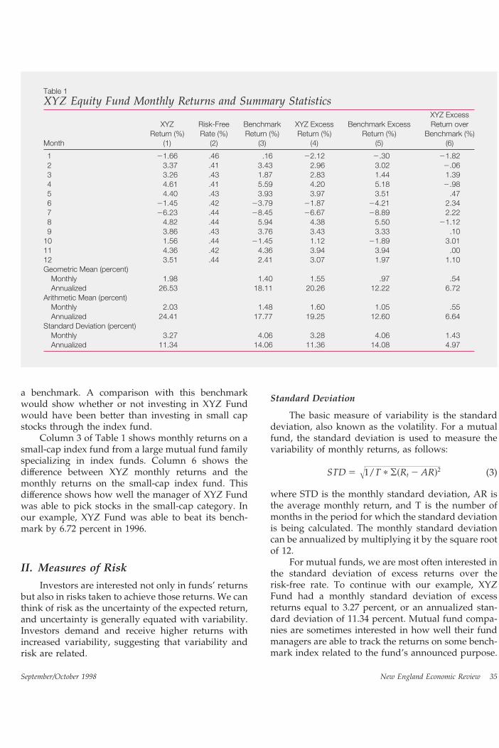
where R is the geometric mean for the period of Tmonths. The industry standard is to report geometricmean return, which is always smaller than the arith-metic mean return. As an illustration, the first columnof Table 1 provides a year of monthly returns for ahypothetical XYZ mutual fund and shows its monthlyand annualized arithmetic and geometric mean returns.
Investors are not interested in the returns of amutual fund in isolation but in comparison to somealternative investment. To be considered, a fundshould meet some minimum hurdle, such as a returnon a completely safe, liquid investment available atthe time. Such a return is referred to as the “risk-freerate” and is usually taken to be the rate on 90-dayTreasury bills. A fund’s monthly return minus themonthly risk-free rate is called the fund’s monthly“excess return.” Column 2 of Table 1 shows therisk-free rate as represented by 1996 monthly returnson a money market fund investing in Treasury bills.Column 4 shows monthly excess returns of XYZ Fund,derived by subtracting monthly returns on the moneymarket fund from monthly returns on XYZ Fund. Wesee that XYZ Fund had an annual (geometric) meanreturn of 20.26 percent in excess of the risk-free rate.
Comparing a fund’s return to a risk-free invest-ment is not the only relevant comparison. Domesticequity funds are often compared to the S&P 500 index,which is the most widely used benchmark for diver-sified domestic equity funds. However, other bench-marks may be more appropriate for some types offunds. Assume that XYZ is a “small-cap” fund,namely, that it invests in small-capitalization stocks,or stocks of companies with a total market value ofless than $1 billion. Since XYZ Fund does not haveany of the stocks that constitute the S&P 500, a moreappropriate benchmark would be a “small-cap” index.Thus, we will use returns on a small-cap index fund as
September/October 1998 New England Economic Review34
a benchmark. A comparison with this benchmarkwould show whether or not investing in XYZ Fundwould have been better than investing in small capstocks through the index fund.
Column 3 of Table 1 shows monthly returns on asmall-cap index fund from a large mutual fund familyspecializing in index funds. Column 6 shows thedifference between XYZ monthly returns and themonthly returns on the small-cap index fund. Thisdifference shows how well the manager of XYZ Fundwas able to pick stocks in the small-cap category. Inour example, XYZ Fund was able to beat its bench-mark by 6.72 percent in 1996.
II. Measures of Risk
Investors are interested not only in funds’ returnsbut also in risks taken to achieve those returns. We canthink of risk as the uncertainty of the expected return,and uncertainty is generally equated with variability.Investors demand and receive higher returns withincreased variability, suggesting that variability andrisk are related.
Standard Deviation
The basic measure of variability is the standarddeviation, also known as the volatility. For a mutualfund, the standard deviation is used to measure thevariability of monthly returns, as follows:
STD 5 Î1/T p (~Rt 2 AR!2 (3)
where STD is the monthly standard deviation, AR isthe average monthly return, and T is the number ofmonths in the period for which the standard deviationis being calculated. The monthly standard deviationcan be annualized by multiplying it by the square rootof 12.
For mutual funds, we are most often interested inthe standard deviation of excess returns over therisk-free rate. To continue with our example, XYZFund had a monthly standard deviation of excessreturns equal to 3.27 percent, or an annualized stan-dard deviation of 11.34 percent. Mutual fund compa-nies are sometimes interested in how well their fundmanagers are able to track the returns on some bench-mark index related to the fund’s announced purpose.
Table 1XYZ Equity Fund Monthly Returns and Summary Statistics
September/October 1998 New England Economic Review 35
This can be measured as the standard deviation ofthe difference in returns between the fund and theappropriate benchmark index. The latter is sometimesreferred to as “tracking error.” In our example, XYZFund had a monthly tracking error of 1.43 percent andan annualized tracking error of 4.97 percent.
Downside Risk
Standard deviation is sometimes criticized as be-ing an inadequate measure of risk because investorsdo not dislike variability per se. Rather, they dislikelosses but are quite happy to receive unexpectedgains. One way to meet this objection is to calculate ameasure of downside variability, which takes accountof losses but not of gains. For example, we couldcalculate a measure of average monthly underperfor-mance as follows: 1) Count the number of monthswhen the fund lost money or underperformed Trea-sury bills, that is, when excess returns were negative.
Investors do not dislikevariability per se. Rather, they
dislike losses but are quitehappy to receive unexpected
gains. Downside risk may be abetter reflection of investors’
attitudes toward risk.
2) Sum these negative excess returns. 3) Divide thesum by the total number of months in the measure-ment period. If we count negative excess returns forXYZ Fund in Table 1, we see it had negative excessreturns in three out of 12 months and their sum was10.66 percent. Thus, its downside risk, measured asaverage monthly underperformance, was 0.89 percent,compared to its monthly standard deviation of 3.27percent.
While downside risk may be a better reflection ofinvestors’ attitudes towards risk, empirical evidencesuggests that the distinction between downside riskand the standard deviation is not as important as itseems because the two measures are highly correlated.Sharpe (1997) analyzed monthly standard deviationsof excess returns and average monthly underperfor-mance in a sample of 1,286 diversified equity funds
in the three-year period between 1994 and 1996. Hefound a close relationship between these two mea-sures, with a correlation coefficient of 0.932. Such aclose correlation is not surprising, since monthly stockreturns generally follow a symmetrical bell-shapeddistribution. Therefore, stocks with larger downsidedeviations will also have larger standard deviations.
A more relevant measure is the ability to predictdownside risk on the basis of both standard deviationand expected returns. Using the same sample of funds,Sharpe found that a regression of average underper-formance on the standard deviation and expectedreturn yields an R-squared of 0.999, which means thatusing only expected returns and standard deviationsof these funds, one can explain 99.9 percent of thevariation in average underperformance.
The average underperformance does not appearto yield much new information over and above thestandard deviation. It is noted here chiefly because it isused by Morningstar, Inc. in its popular ratings ofmutual funds, Morningstar ratings, which are dis-cussed in the next section.
Value at Risk
In recent years, Value at Risk has gained promi-nence as a risk measure. Value at Risk, also known asVAR, originated on derivatives trading desks at majorbanks and from there spread to currency and bondtrading. Its popularity was much enhanced by the1993 study by the Group of Thirty, Derivatives: Prac-tices and Principles, which strongly recommended VARanalysis for derivatives trading. Essentially, it answersthe question, “How much can the value of a portfoliodecline with a given probability in a given timeperiod?” The period used in measuring VAR for abank’s trading desk ranges from one day to twoweeks, while the probability level is usually set in therange of 1 to 5 percent. Therefore, if we choose aperiod of one week and a probability level of 1 per-cent, a portfolio with a VAR of 5 percent might lose 5percent or more of its value no more than 1 percent ofthe time. VAR is not a measure of maximum loss;instead, for given odds, it reports how great the rangeof losses is likely to be.
We will use the example of XYZ Fund returns toillustrate the simplest version of VAR calculation.Suppose that an investor put $1,000 into XYZ Fundand wishes to know the VAR for this investment forthe next month. We can easily answer this question ifwe make certain assumptions about the statisticaldistribution of the fund’s returns.
September/October 1998 New England Economic Review36
The most common assumption is that returnsfollow a normal distribution. One of the properties ofthe normal distribution is that 95 percent of all obser-vations occur within 1.96 standard deviations from themean. This means that the probability that an obser-vation will fall 1.96 standard deviations below themean is only 2.5 percent. For the purposes of calculat-ing VAR we are interested only in losses, not gains, sothis is the relevant probability. Recall that XYZ Fundhad an (arithmetic) average monthly return of 2.03percent and a standard deviation of 3.27 percent.Thus, its monthly VAR at the 2.5 percent probabilitylevel is 2.03% 2 1.96 p 3.27 5 24.38%, or $43.80 for a$1,000 investment, meaning that the probability oflosing more than this is 2.5 percent.
VAR is often said to have an advantage over otherrisk measures in that it is more forward-looking. Forexample, in a recent article in Risk Magazine, Glauber(1998) describes the advantages of using VAR in thisway: “A common analogy is that without VAR, man-agement has to drive forward by looking out of therear window. All the information available is aboutpast performance. By using VAR management can usethe latest tools to keep their eyes firmly focused infront.”
While it can be described as forward-looking,VAR still relies on historical volatilities. However, thestrength of VAR models is that they allow us toconstruct a measure of risk for the portfolio not fromits own past volatility but from the volatilities of riskfactors affecting the portfolio as it is constituted today.Risk factors are any factors that can affect the value ofa given portfolio. They include stock indexes, interestrates, exchange rates, and commodity prices. A mea-sure based on risk factors rather than on the portfolio’sown volatility is especially important for funds thatrange far and wide in their choice of investments, usefutures and options, and abruptly change their com-mitments to various asset classes. (This descriptionapplies to many hedge funds, though not perhaps tomany of the regular mutual funds available to retailinvestors.)
Clearly, if the present composition of the fund’sportfolio is significantly different than it was duringthe past year, then historical measures would notpredict its future performance very accurately. How-ever, as long as we know the fund’s current com-position and can assume that it will stay the sameduring the period for which we want to know theVAR, we can use a model based on the historicaldata about the risk factors to make statistical infer-ences about the probability distribution of the fund’s
future returns. In fact, for certain portfolios it isnecessary to have a model based on risk factors evenif one does not trade the portfolio at all. This isparticularly true for portfolios consisting of bondsand/or options and futures, because such portfolios“age,” that is, their characteristics change from thepassage of time alone. In particular, as bonds ap-proach maturity, their value approaches face valueand their volatility diminishes and disappears alto-gether at maturity, when the bond can be redeemed atface value. Options, on the other hand, tend to losevalue as they approach expiration, all other thingsbeing equal. This is one of the reasons why VARanalysis is used more frequently in derivatives andfixed-income investment and is less widespread forequities.
VAR answers the question,“How much can the valueof a portfolio decline witha given probability in a
given time period?”
Nevertheless, VAR models can provide usefulinformation for equities also. For example, the man-ager of XYZ Fund can consider all the stocks currentlyin the portfolio to be separate risk factors. As long asthe manager has the data on past returns for eachstock, he can estimate their volatilities and correla-tions. This will enable the manager to calculate theVAR of the portfolio as it exists at the moment,not as it has been in the past. Risk managers at mutualfund companies may also be interested in the valueat risk as it applies to underperforming the fund’schosen benchmark. This measure, known as “relative”or “tracking” VAR, can be thought of as the VARof a portfolio consisting of long positions in all thestocks the fund currently owns and a short positionin the fund’s benchmark. While VAR provides aview of risk based on low-probability losses, forsymmetrical bell-shaped distributions such as thosetypically followed by stock returns, VAR is highlycorrelated with volatility as measured by the stan-dard deviation. In fact, for normally distributed re-turns, value at risk is directly proportional to standarddeviation.
September/October 1998 New England Economic Review 37
III. Risk-Adjusted Performance
Two risk measures discussed in the previoussection, namely the standard deviation and the down-side risk, have been used to adjust mutual fundreturns to obtain measures of risk-adjusted perfor-mance. This section describes two measures of risk-adjusted performance based on the standard devia-tion, namely, the Sharpe ratio and the Modiglianimeasure, and Morningstar ratings, which are based ondownside risk.
Sharpe Ratio
The most commonly used measure of risk-ad-justed performance is the Sharpe ratio (Sharpe 1966),which measures the fund’s excess return per unit of itsrisk. The Sharpe ratio can be expressed as follows:
Sharpe ratio
5fund’s average excess return
standard deviation of fund’s excess return . (4)
Column 4 of Table 1 shows that the (arithmetic)monthly mean excess return of XYZ Fund is 1.60percent, while the monthly standard deviation of itsexcess return is 3.28 percent.1 Thus, the fund’smonthly Sharpe ratio is 1.60%/3.28% 5 .49. Theannualized Sharpe ratio is computed as the ratio ofannualized mean excess return to its annualized stan-dard deviation, or, equivalently, as the monthlySharpe ratio times the square root of 12. Thus, XYZ’sannualized Sharpe ratio is 19.25%/11.36% 5 1.69.
The Sharpe ratio is based on the trade-off betweenrisk and return. A high Sharpe ratio means that thefund delivers a lot of return for its level of volatility.The Sharpe ratio allows a direct comparison of therisk-adjusted performance of any two mutual funds,regardless of their volatilities and their correlationswith a benchmark.
It is important to keep in mind that the relevanceof a risk-adjusted measure such as the Sharpe ratio forchoosing a mutual fund depends critically on inves-tors’ ability to do two things: 1) combine an invest-ment in a mutual fund with an investment in the
riskless asset, and 2) leverage the investment by, forexample, borrowing money to invest in the mutualfund. (For the result to hold exactly, the investor mustbe able to borrow and lend at the same risk-free rate.)This is because the combination of investing in anygiven mutual fund and in a riskless asset allows one tolower the risk of the combined investment at the priceof the corresponding reduction in expected return.Alternatively, leveraging one’s investment in the fundallows one to increase expected return at the price ofthe corresponding increase in risk. Thus, any level ofrisk can be achieved with the given fund, and so theinvestor can achieve the best combination of risk andreturn by investing in the fund with the highestSharpe ratio, regardless of the investor’s own degreeof risk tolerance.2
As an example, consider an investor who has$1,000 to invest and is choosing whether to invest inFund X or Fund Y (but not both). Fund X has anexpected excess return of 12 percent and a standarddeviation of 9 percent. Fund Y has an expected excessreturn of 6 percent and a standard deviation of 4percent. Fund X has a Sharpe ratio of 1.33 while FundY has a Sharpe ratio of 1.5. Because Fund Y has ahigher Sharpe ratio it is a better choice, even forinvestors who wish to earn an expected excess returnof 12 percent. Instead of investing in Fund X, thoseinvestors can borrow another $1,000 and invest theresulting $2,000 in Fund Y. (See point Y9 on Figure 1.)This leveraged investment provides twice the risk andtwice the expected return of unleveraged investmentin Fund Y, namely expected excess return of 12percent and a standard deviation of 8 percent, betterthan the 9 percent standard deviation the investorcould get by investing in Fund X. Figure 1 shows theserisk/return combinations. The slopes of the linesdrawn from the origin through the points representingrisk and return of Funds X and Y are equal to thefunds’ Sharpe ratios. Clearly, all funds that lie along ahigher line are better investments than the funds on alower line, so that a fund with a higher Sharpe ratio ispreferable to a fund with a lower one.
Despite its near universal acceptance among aca-demics and institutional investors, the Sharpe ratio isnot well known among the general public and finan-cial advisors. A recent newspaper column, comment-
1 Academic literature generally uses the arithmetic mean in thecalculation of the Sharpe ratio because of its better statisticalproperties. For example, the Sharpe ratio based on the arithmeticmean times the square root of the number of observations can beinterpreted as a T-statistic for the hypothesis that the fund’s excessreturn is significantly different from zero.
2 This is exactly the conclusion of the Capital Asset PricingModel (CAPM), which holds that a portfolio of assets exists (knownas the market portfolio) that provides the highest return per unit ofrisk and is appropriate for all investors. The CAPM is discussed inmore detail in the next section.
September/October 1998 New England Economic Review38
ing on the contents of the CFP (Certified FinancialPlanner) examination, had this to say about the Sharperatio:
But I do not know of a single financial planner—and Iasked dozens of them after taking the test—who has everhad a client come in and ask for the calculation of SharpeMeasure of Performance on a mutual fund. In fact, noneof the planners I queried could actually calculate theSharpe Index without the formula in front of them. (TheSharpe is so esoteric that most mainstream financialdictionaries ignore it, most planners can’t adequatelyexplain it, and I am not even going to attempt it here.) Yetthe Sharpe Index is on the CFP exam (Jaffe 1998).
Modigliani Measure
The view that the Sharpe ratio may be too difficultfor the average investor to understand is shared byModigliani and Modigliani (1997), who propose asomewhat different measure of risk-adjusted perfor-mance. Their measure expresses a fund’s performancerelative to the market in percentage terms and theybelieve that the average investor would find the
measure easier to understand. The Modigliani mea-sure can be expressed as follows:
Modiglianimeasure 5
fund’s average excess returnstandard deviation of fund’s excess return
3 standard deviation of index excess return. (5)
Modigliani and Modigliani propose to use the stan-dard deviation of a broad-based market index, suchas the S&P 500, as the benchmark for risk comparison,but presumably other benchmarks could be used. Inessence, for a fund with any given risk and return,the Modigliani measure is equivalent to the return thefund would have achieved if it had the same risk as themarket index. Thus, the fund with the highest Modigli-ani measure, like the fund with the highest Sharperatio, would have the highest return for any level ofrisk. Since their measure is expressed in percentagepoints, Modigliani and Modigliani believe that it canbe more easily understood by average investors.
To continue with our example of XYZ Fund, itsannualized mean (arithmetic) excess return is 19.25percent and its annualized standard deviation is 11.36percent. If the standard deviation of the excess returnon the S&P 500 market index is 15 percent, XYZ’sModigliani measure is 19.25%/11.36% 3 15% 525.42%. This 25.42 percent return can be interpreted asfollows: An investor who is willing to accept thehigher standard deviation of the S&P500 can improvehis return by investing in XYZ and leveraging thatinvestment to achieve the standard deviation of 15percent. This would result in the return of 25.42percent, which is the fund’s Modigliani measure.Performance measures for the XYZ Fund are summa-rized in Table 2.
As the preceding example makes clear, theModigliani measure has the same limitation as theSharpe ratio in that it is of limited practical use toinvestors who are unable to use leverage in their
Table 2Risk-Adjusted Performance Measures forXYZ Fund
Alpha Sharpe RatioModigliani
Measure (%)
Monthly .803 .49 1.98Annualized 9.63 1.69 25.42
September/October 1998 New England Economic Review 39
mutual fund investing. As the Modigliani measureis very new, it remains to be seen if it will meet withmore understanding and acceptance than the Sharperatio.
Morningstar Ratings
Morningstar, Incorporated, calculates its ownmeasures of risk-adjusted performance that form thebasis of its popular star ratings.3 Star ratings are wellknown among individual investors. One study foundthat 90 percent of new money invested in equity fundsin 1995 flowed to funds rated 4 or 5 stars by Morning-star (Damato 1996).
For the purpose of its star ratings, Morningstardivides all mutual funds into four asset classes—domestic stock funds, international stock funds, tax-able bond funds, and municipal bond funds. First,Morningstar calculates an excess return measure foreach fund by adjusting for sales loads and subtractingthe 90-day Treasury bill rate. These load-adjustedexcess returns are then divided by the average excessreturn for the fund’s asset class.4 This can be summa-rized as follows:
Morningstar return
5load-adjusted fund excess return
average excess return for asset class . (6)
Second, Morningstar calculates a measure of down-side risk by counting the number of months in whichthe fund’s excess return was negative, summing up allthe negative excess returns and dividing the sum bythe total number of months in the measurement pe-riod. The same calculation of average monthly under-performance is then done for the fund’s asset class asa whole. Their ratio constitutes Morningstar risk:
Morningstar risk
5fund’s average underperformance
average underperformance of its asset class . (7)
Third, Morningstar calculates its raw rating by sub-tracting the Morningstar risk score from the Morning-star return score. Finally, all funds are ranked by theirraw rating within their asset class and assigned their
stars as follows: top 10 percent—5 stars; next 22.5percent—4 stars; middle 35 percent—3 stars; next 22.5percent—2 stars; and bottom 10 percent—1 star. Starsare calculated for three-, five-, and 10-year periods andthen combined into an overall rating. Funds with atrack record of less than three years are not rated.
In addition to its star ratings, Morningstar alsocalculates category ratings for each fund. The maindifference between stars and category ratings is thatcategory ratings are not based on four asset classes buton more narrowly defined categories, with each fundassigned to one (and only one) category among 44altogether: 20 domestic stock categories, 9 interna-tional stock categories, 10 taxable bond categories, and5 municipal bond categories. In addition, categoryratings are not adjusted for sales load and are calcu-lated only for a three-year period.
Relationships among Performance Measures
An important question in comparing perfor-mance measures is whether or not they would lead toa similar ranking of mutual funds. The first thing tonote is that, as long as one uses the same benchmark,
3 The following description is based on Harrel (1998).4 When average excess return for the asset class is negative, the
T-bill rate is substituted in the denominator.
September/October 1998 New England Economic Review40
any rankings of funds based on the Sharpe ratio andthe Modigliani measure would be identical (Modig-liani and Modigliani 1997). From Equations 4 and 5,it is clear that the Modigliani measure can be ex-pressed as the Sharpe ratio times the standard devia-tion of the benchmark index, so that the two measuresare directly proportional.
A more interesting comparison is between theSharpe ratio and Morningstar ratings. Morningstarratings differ from the Sharpe ratio in that they mea-sure performance relative to a peer group—either abroad asset class as in the star ratings or a narrowerpeer group such as one of the 44 categories—so thatthe rankings could differ considerably. To find out ifthey produce similar results, we compared the corre-lations between Sharpe ratios and Morningstar starratings for 3,308 funds for the three-year period of1995 to 1997. The sample consisted of 1,737 domesticequity funds, 442 international stock funds, and 1,129taxable bond funds, as classified by Morningstar. Weincluded all such funds found in the Financial Re-search Corporation data base with at least three yearsof performance data.
The funds were ranked into percentiles within
their respective asset classes, first, according to theirSharpe ratios and, second, according to their Morn-ingstar star ratings. The three panels in Figure 2 showa fund’s percentile based on its three-year star ratingon the horizontal axis plotted against its percentilebased on the three-year Sharpe ratio on the verticalaxis. We see that all three types of funds exhibitedimpressively high correlations between their percen-tiles as judged by the two measures. Internationalequity funds had the highest correlation, with a cor-relation coefficient of 0.979. Domestic equity funds hada slightly lower correlation coefficient of 0.947, whiletaxable bond funds had a correlation coefficient of.845.
Earlier empirical work also found high correla-tions among performance measures. Sharpe (1997)compared rankings based on Morningstar categoryratings, Morningstar star ratings, and Sharpe ratios ina sample of 1,286 diversified domestic stock fundsduring the three-year period between 1994 and 1996.The ranking of the funds based on star and categoryratings had a correlation coefficient of 0.957. Rankingsbased on Sharpe ratios and category ratings had acorrelation coefficient of 0.986, while those based on
Sharpe ratios and Morningstar star ratings had acorrelation coefficient of 0.955.5
IV. Modern Portfolio Theory
The measures of risk-adjusted performance dis-cussed above are subject to the same limitation as therisk measures on which they are based, namely, thatthey describe each fund in isolation and not in termsof its contribution to the investor’s existing portfolio.For example, the Sharpe ratio can be used by aninvestor to choose one fund in combination with eitherborrowing or investing in the risk-free asset, depend-ing on the investor’s degree of risk tolerance. How-ever, because the Sharpe ratio does not take intoaccount correlations between fund returns, this wouldnot be the best way for an investor to choose severalmutual funds or to add a fund to an existing portfolio.Recall that in the example in the previous section, aninvestor had to choose between Fund X and Fund Y.Fund Y was the better choice in combination with aninvestment in a risk-free asset than Fund X becauseFund Y had a higher Sharpe ratio. However, as long asthe returns on X and Y were not perfectly correlated,the investor could do even better with a combinationof Funds X and Y and the riskless asset.
It is easy enough to find the efficient portfolio offunds (the one with the lowest risk for a given level ofexpected return) when one has a choice of a few funds,but it is not so easy to do with a choice of thousandsof funds. One way around this problem is provided bymodern portfolio theory, first developed by Marko-witz (1952). It introduces the concept of the “marketportfolio,” that is, the portfolio consisting of everysecurity traded in the market held in proportion to itscurrent market value. Moreover, modern portfoliotheory divides the risk of each security (or eachportfolio of securities such as a mutual fund) intotwo parts: systematic and unsystematic. Systematicrisk (or market risk) is the risk associated with thecorrelation between the return on the security and thereturn on the market portfolio. Unsystematic risk(also known as specific risk) is the “leftover” risk,which is associated with the variability of returns ofthat security alone. The distinction between the two
components of risk is important because they behavedifferently as one increases the number of securities inthe portfolio. The unsystematic component of risk canbe diversified away because it gets “averaged out” asthe number of securities gets larger, and so it can beignored in a well-diversified portfolio. Systematic risk,on the other hand, cannot be diversified away andinvestors expect to be compensated for bearing it.
The distinction between systematic and unsys-tematic risk is the foundation of the Capital AssetPricing Model (CAPM) developed by Sharpe (1964)and Lintner (1965). The CAPM states that the expectedreturn on a given security or portfolio is deter-mined by three factors: the sensitivity of its return tothat of the market portfolio (known as beta), the returnon the market portfolio itself and the risk-free rate.(See the Box for a more detailed discussion of theCAPM.)
Empirical Estimates of Beta
The beta can be estimated empirically from a timeseries of the historical returns on a given investmentand the historical returns on the market portfolio. Fiveyears of monthly returns (60 months) are commonlyused to estimate beta. The return on the marketportfolio is traditionally represented by the return onthe S&P 500, though a value-weighted index of allsecurities in the market may be preferable, given thedefinition of the market portfolio.
The most common way to estimate beta is a linearregression of the excess return of the given portfolioon the excess return of the market portfolio, wherebeta is the slope of the regression line:
Rp 2 Rf 5 a 1 b~Rm 2 Rf! 1 ep (8)
Alpha is the intercept of that regression and can beinterpreted as the “extra” return for the fund’s level ofsystematic risk, or the “value added” by the fund’smanager. This interpretation of alpha as a measure ofperformance adjusted for systematic risk was firstsuggested by Jensen (1968). However, it is importantto be careful in the way one interprets this measure inthe CAPM framework. In theory, any alpha other thanzero is inconsistent with the CAPM because, if themarket portfolio is efficient, then the expected returnon every security or portfolio of securities is com-pletely determined by its relationship to the marketportfolio, as measured by beta. Thus, it is logicallyinconsistent to apply the CAPM to measure a mutualfund’s return over and above the return required tocompensate investors for the fund’s systematic risk,
5 Sharpe finds that correlations between Sharpe ratios andMorningstar measures tend to be high when the average fundperforms well and the funds have returns and risks tightly clusteredaround the average fund. Conversely, the correlations are lowerwhen the average fund does poorly and the funds display morevariability around the average.
September/October 1998 New England Economic Review42
since according to the CAPM it is impossible to earnsuch extra return. On the other hand, if investors haveportfolios that are markedly different from the marketportfolio, then a fund’s alpha and beta found withreference to the market portfolio may not be relevantfor them.
Thus far, we seem to have come to a paradoxicalconclusion: We can measure the risk and the risk-adjusted return of a mutual fund on an individualbasis by using measures such as the standard devia-tion and the Sharpe ratio, but this measure does nottake account of the effects of diversification. Alterna-tively, we can use the empirical form of the CAPM toderive the fund’s alpha and beta with respect to themarket portfolio. However, the CAPM implies that allinvestors hold the market portfolio, in which casethere is no point in analyzing mutual funds, since theywould all be inferior to the market portfolio. Also, ifthe market portfolio is not efficient for all investors,then they would hold different portfolios and alphaand beta may be no more relevant than a simpleSharpe ratio. In theory, an investor can construct anindividual efficient portfolio out of mutual funds,subject to the investor’s tax status, expectations, hold-ings of illiquid assets, and so on. But with 5,000 fundsto choose from, an investor would have to consider12.5 million correlations between them to find theefficient portfolio. An even more basic problem formany investors is simply to know what assets theyhold in their portfolios at any given time. For aninvestor with half a dozen funds each holding hun-dreds of securities, it is not a trivial problem to knowwhat the portfolio consists of, let alone how efficient itis or whether it resembles the market portfolio, how-ever defined.
Asset-Class Factor Models
It is generally agreed that a large part of thedifferences in investors’ portfolio returns can be ex-plained by the allocation of the portfolio among keyasset classes. Thus, it is not crucial to consider eachindividual security separately for inclusion in theportfolio. Instead, one can use an asset-class factormodel to evaluate the performance of portfolio man-agers and construct a portfolio of mutual funds. To doso, one must first define the “key” asset classes andmeasure how sensitive mutual fund returns are to thevariations in asset-class returns.
For example, an asset-class model might includethe following: Treasury bills, intermediate-term gov-ernment bonds, long-term government bonds, corpo-
rate bonds, mortgage-based bonds, non-U.S. bonds,U.S. stocks, European stocks, and Asia/Pacific stocks.What makes a “good” asset-class model? Accordingto Sharpe (1992), while not strictly necessary, it isdesirable for asset classes to be mutually exclusiveand exhaustive and to have returns that “differ.” Thismeans that no security should be in more than oneasset class, as many securities as possible should be
Generally, a good model of assetclasses is the one that can
explain a large portion of thevariance of returns on the assets.
included in a given asset class, and asset returns ondifferent classes of assets should have low correlationsand, if this is not possible, different standard devia-tions. Generally, a good model of asset classes is theone that can explain a large portion of the variance ofreturns on the assets. If two models can explain thisvariance equally well, the one with fewer asset classesis preferable because fewer classes are more likely torepresent stable economic relationships. An additionalpractical consideration is that widely available, reli-able indexes that could be used as benchmarks shouldrepresent the returns on each class of assets accurately.
Constructing a Benchmark
If the asset classes span the market portfolio, theinvestor still has the problem of comparing the returnson his mutual funds to the return on the wholecollection of asset classes. It would be convenient if theinvestment objectives of every fund neatly corre-sponded to one asset class. In this case, the indexrepresenting the asset class in question would be anappropriate benchmark for measuring the fund’s per-formance. For example, the Russell 1000 index couldbe used as a benchmark for a fund invested inlarge-capitalization U.S. stocks, while the MSCI EAFE(Europe/Australia/Far East) Index could be used tobenchmark an international stock fund. However, thisone-to-one correspondence rarely happens. Manyfunds invest in a number of asset classes and findingan appropriate benchmark consisting of a “blend” ofappropriate indexes is not a straightforward exercise.Some funds shift their asset allocation through time,
September/October 1998 New England Economic Review 43
which further complicates the issue. Consider, forexample, a balanced fund that is invested 50 percent inU.S. common stocks and 50 percent in U.S. long-termgovernment bonds. Suppose also that during the pastfive years the fund’s stock allocation ranged from 30percent to 70 percent depending on the manager’sview of the market. We could try to construct abenchmark that would mimic the fund’s shifts in assetallocation through time. However, such a benchmarkwould be of questionable value to an investor, even ifit were possible to know a fund’s asset allocation atany given moment. To be useful, a benchmark for thefund’s performance should be a viable investmentstrategy that can be followed by an investor at a lowcost and it should not depend upon the benefit ofhindsight. For example, a strategy consisting of invest-ing in a mix of index funds and holding this mix forfive years would meet these requirements.
A fixed benchmark can be constructed usingeither a historical or a hypothetical approach. To use ahistorical benchmark we would estimate the fund’saverage asset allocation throughout the last five yearsand compare a return on this asset mix to the fund’sown return. A hypothetical approach would be to usethe fund’s current asset allocation (in this case halfstocks and half bonds) and compare the performanceon this mix over the last five years to the fund’s actualperformance. Note that neither of these approacheswould require an investor to trade in and out of assetclasses.
Often, we do not know the fund’s asset allocation.At present, the mutual fund prospectus describes thefund’s investment goals, as well as any restrictions onthe fund’s portfolio composition, such as the abilityto use derivatives. However, the description of thefund’s goals often is not specific enough to enable
The Capital Asset Pricing Model
The Capital Asset Pricing Model rests on anumber of simplifying assumptions. All investorsare assumed to be risk averse and to have identicalpreferences about risk and return. Investors areassumed to care only about risk and return, so thattheir utility function admits only the mean and the
variance of the distribution of returns. In addition,the model assumes that all investors have identicalexpectations about the future risks and returns ofall securities, have the same tax rates, and are ableto borrow and lend at the risk-free rate withoutlimits on the amounts borrowed or lent, and that norisky assets are excluded from the investment port-folio. Finally, the model assumes that there are notransaction costs and no costs of research.
To see the implications of this more clearly, wecan plot the risks against the expected returns of anumber of possible portfolios, as shown in FigureB-1. Among all possible portfolios there will bethose where no other combination of (risky) assetswould produce a better return for the same level ofrisk, or equivalently, lower risk for the same return.Such portfolios are known as mean-variance effi-cient. If we plot a line through them, the result willbe the “efficient frontier,” as shown in Figure B-1. Ifno borrowing or lending was allowed, all investorswould hold one of these efficient portfolios, de-pending on their risk tolerance. However, if bor-rowing and lending are possible, investors can doeven better than being somewhere on the efficientfrontier. We can see this clearly if we draw atangent from the efficient frontier starting at therisk-free rate. If investors hold a combination ofrisky securities that is the same as the one where the
�������
������
�����������������
September/October 1998 New England Economic Review44
the investor to assign a specific mix of asset classes tothe fund with any degree of precision. In addition tothe disclosures found in the prospectus, the SECrequires management to disclose the list of securitiesowned by the fund every six months. In principle, bystudying this list of securities the investor can deter-mine to which class each belongs and, thus, determinethe fund’s asset allocation. This approach has twoproblems, however. First, each fund typically holdshundreds of securities and categorizing each one is adifficult and time-consuming task. Second, the inves-tor would be looking at the fund composition sixmonths ago, which may not necessarily represent itscomposition now or in the future. Reporting holdingson a more timely basis would not be an acceptablesolution, however. For competitive reasons, manyfunds regard their current holdings as proprietaryinformation. Disclosing them can hurt the fund’s
performance by enabling other market participants totrade against them, especially if some positions arelarge or illiquid.
Thus, it is often necessary to construct a bench-mark for the fund’s asset allocation without knowingthe fund’s actual holdings. If the fund does not shift itsasset allocation through time, it is possible to analyzeits historical performance with respect to a number ofpreviously defined asset classes. For example, one canregress the fund’s monthly returns on the monthlyreturns to the indexes chosen to represent asset classesfor the set amount of time, say 60 months, as shown inEquation 9:
Rp 2 Rf 5 b1~R1 2 Rf! 1 b2~R2 2 Rf! 1 . . .
1 bn~Rn 2 Rf! 1 ep (9)
where Rp is the expected return on the fund, Rf is the
line is tangent to the efficient frontier, they canachieve any desired trade-off of risk and return thatis possible along that line. This line is known as thesecurity market line and it is also shown in FigureB-1. Borrowing and lending make it possible toseparate investors’ preferences about risk and re-turn from the opportunities available in the capitalmarket. Thus, each investor would hold the sameportfolio of risky assets (the market portfolio) andonly the mix of the market portfolio and the risk-free asset would vary.
If the model were literally true and all investorsheld the same mix of risky assets, talking aboutmeasuring risk or performance of mutual fundswould be pointless. In fact, only one mutual fundwould exist, the universal index fund consisting ofthe market portfolio; any fund consisting of adifferent combination of risky assets would beinferior. Recall that this is the same line of reason-ing we used in describing why the Sharpe ratio (orthe Modigliani measure) is the relevant measure ofrisk-adjusted performance. The Sharpe ratio mea-sures the amount of expected excess return per unitof risk. If investors can borrow and lend, they caninvest in the portfolio with the highest Sharpe ratioand mix it with the risk-free asset in differentproportions. Thus, it follows that if the CAPMholds, then the market portfolio is, in fact, theportfolio with the highest Sharpe ratio.
Two problems arise in applying the CAPM to
real-world investment. One problem concerns thedefinition of the “market portfolio,” and the second,the definition of the “efficient portfolio.” Roll (1977)pointed out that the CAPM can never be definitelytested because, as a practical matter, it is impossibleto define the “market portfolio” with any degree ofprecision. Should foreign assets be included? Howabout commodities? Real estate? Antiques? Art?Some of these assets are traded so infrequently thatit would be quite difficult to construct a reliableseries of monthly returns. Finally, some assets, suchas the present value of the investor’s labor income,cannot be traded at all, yet they constitute animportant part of the investor’s overall “portfolio.”Generally, as the definition of the “market” be-comes broader, the estimate of its monthly returnsbecomes less reliable.
The second problem is that no one truly “effi-cient” portfolio exists that would be appropriate forall investors. Because research is costly, not allinvestors have access to the same information, nordo they have the same opinions and beliefs. As longas investors have differing expectations about thefuture risks and returns of various investments,they will not agree on the same “efficient” portfoliobut rather choose securities that have the bestprospects according to their own judgment. In thiscase, instead of being efficient in some absolutesense, the market portfolio balances the divergentassessments of all investors (Lintner 1965).
September/October 1998 New England Economic Review 45
return on the risk-free asset, R1 through Rn are thereturns on asset classes 1 through n, and b1 through bnare the corresponding investments of Rp to these assetclasses. Finally, ep is the residual, or non-factor, returnon the fund. It can be seen as the “value added” (orsubtracted, as the case may be) by the fund managerrelative to the return the investor could get by invest-ing in a benchmark consisting of index funds repre-senting the same asset classes.
The resulting slope coefficients would then repre-sent the sensitivities of the fund’s returns to thereturns of the corresponding asset classes. However,the results of such regressions are often difficult tointerpret, because the coefficients do not sum to oneand often some coefficients turn out to be negative.Mutual funds normally do not take short positions inasset classes and their investments in various assetsshould sum to 100 percent. Thus, to be meaningful,
A large part of the differences ininvestors’ portfolio returns can beexplained by the allocation of theportfolio among key asset classes.
coefficients should be constrained to be positive orzero and to sum to one. The presence of inequalityconstraints (0 # bi # 100%) necessitates the use ofquadratic programming for the estimation of thefund’s exposure to the asset classes. This method,introduced by Sharpe, has become known as “styleanalysis.” It involves finding the set of asset classexposures (bis) that minimize the variance of thefund’s residual return VAR(ep) and are consistentwith the above constraint. Note that style analysisrepresents a form of historical approach, which esti-mates the fund’s average exposure to asset classesduring the period analyzed.
Yet another approach to estimating risk and per-formance of mutual funds was recommended by theFinancial Economists Roundtable in its “Statement onRisk Disclosure by Mutual Funds” issued in Septem-ber 1996. This approach is future oriented because itcalls for disclosure by fund managers of asset alloca-tions they plan to have in their funds for a specifiedfuture period. Specifically, the Roundtable recom-mended that funds use narrowly defined asset classesfor this disclosure, rather than broad ones like the
S&P 500. The statement listed 14 possible asset classesthat are represented well by available indexes andsuggested that funds specify not just one index, buta portfolio of indexes, whenever appropriate. TheRoundtable also recommended that funds reporthistorical comparisons of their returns with the re-turns that could have been obtained by investing in anindex fund or a portfolio of index funds correspond-ing to their previously announced index or blend ofindexes. This information would be sufficient to eval-uate whether or not a given fund fits the investor’sportfolio in terms of asset allocation and, if it does,whether the investor would be better off investing inthe fund or in an index fund representing the sameasset class.
Another performance measure that is derivedfrom comparing a fund to its benchmark is the “infor-mation ratio,” defined as follows:
Information ratio
5fund return 2 benchmark return
standard deviation ~fund return 2 benchmark return!.
(10)
This is another version of the Sharpe ratio, whereinstead of dividing the fund’s return in excess of therisk-free rate by its standard deviation, we dividethe fund’s return in excess of the return on thebenchmark index by its standard deviation. The infor-mation ratio can be thought of as a more generalmeasure of which the “regular” Sharpe ratio is aspecial case with the return on Treasury bills used asthe benchmark for all funds. It should be noted that aranking of funds based on the information ratio willgenerally differ from the one based on the regular, orexcess return, Sharpe ratio, and its relevance to aninvestor’s decision-making is not obvious.
V. Summary and Conclusion
Portfolio theory teaches us that investmentchoices are made on the basis of expected risks andreturns. These expectations are often formed on thebasis of a historical record of monthly returns, mea-sured for a period of time. For mutual funds, commonmeasures include average excess return (total monthlyreturn less the monthly return on Treasury bills) andits standard deviation, tracked for a sufficient length oftime, such as three or five years. A fund’s risk andreturn can be combined into one measure of risk-
September/October 1998 New England Economic Review46
adjusted performance by dividing the average excessreturn by the standard deviation. The resulting mea-sure, known as the Sharpe ratio, can help the investorto identify the most “efficient” fund, namely the onewith the highest return per unit of risk. However, auniversal measure such as the Sharpe ratio is useful asa guide to investment decisions only in a limited set ofcircumstances. In particular, the measure is useful toinvestors who are putting all their money into onediversified fund and are able to use leverage or investin the risk-free asset.
Much more common is the situation where aninvestor constructs a portfolio of funds or adds a fundto an existing portfolio. In this case, the fund’s mar-ginal contribution to the portfolio’s risk and returnis more important than its individual characteristics.To construct an efficient portfolio, an investor musttake account of the correlations among the invest-ments being considered. The Capital Asset PricingModel implies that under certain assumptions, theefficient portfolio is the same for all investors and inthe aggregate constitutes the market portfolio. Takenliterally, this implies that all investors should invest ina universal index fund. Because it is efficient, theuniversal index fund would, by definition, have thehighest Sharpe ratio of all mutual funds.
Among the reasons why this does not happen isthe fact that both “efficient” portfolio and “market”portfolio are difficult to define in practice. In particu-lar, because of their different tax treatments, assess-ments of future asset returns, and endowments ofnon-tradable assets, investors cannot all have the sameefficient portfolio. For example, an owner of a privatebusiness who has a substantial part of his wealth tiedup in the business will have very different needs fordiversification than someone who does not. Similarly,the “market portfolio” is an abstraction. In theory, itshould consist of a value-weighted index of all assets,but many assets are illiquid or non-tradable and theirprices are not known with any certainty.
Despite these caveats, the main insight of theCAPM remains sound: For the aggregate supply of allsecurities in the market to equal the aggregate de-mand for these securities, their expected returns mustcompensate investors for systematic risk. These re-turns tell an investor how much he can expect to berewarded for bearing the systematic risk of a givensecurity or fund. This approach has led to the use ofrisk-adjusted excess return (alpha) as a measure ofperformance. The excess return implies that the man-ager of that fund has delivered a return over andabove that which is required to compensate investors
for bearing market risk, where the market is repre-sented as a broad-based index such as the S&P 500.
A different version of alpha is measured against aspecific benchmark for the fund, rather than againstthe market as a whole. Similarly, a benchmark-relatedversion of the Sharpe ratio, known as the informationratio, is based on excess returns over the benchmarkrather than the risk-free rate. An investor can thenchoose one or more funds with the highest alphas orinformation ratios in their categories. However, if thecategories themselves and their shares in the inves-tor’s portfolio are chosen arbitrarily, the resultingportfolio can be highly inefficient. This is because theexcess return measured by the benchmark alpha isrelated not to the market risk of the fund, but to its
To be useful, a benchmark for afund’s performance should be aviable investment strategy that
can be followed by an investor ata low cost and it should not
depend on the benefit of hindsight.
“risk” relative to the benchmark. This, however, tellsus nothing about the expected return and risk of thebenchmark itself. Similarly, the information ratio usesthe “tracking error,” or the standard deviation of thedifference between the fund return and the benchmarkreturn, which is of questionable relevance as a mea-sure of risk for most investors.
An approach known as asset allocation divides allsecurities into several asset classes and tries to con-struct an efficient portfolio based on expected returns,risks, and correlations of indexes representing theseasset classes. In this context, an “efficient” portfolio issimply a portfolio invested in the benchmark indexesin such a way that no other combination of theseindexes would result in a portfolio with a higherreturn for a given level of risk. It should be empha-sized, however, that this is not a fully efficient portfo-lio because information about correlations among in-dividual securities within an index and across theindexes is lost in the transition from individual secu-rities to the benchmarks that represent them.
It is quite likely that a more efficient portfolio can
September/October 1998 New England Economic Review 47
be constructed directly from funds that are not thebest performers in their categories because they offsetone another’s risks better. However, the logisticalproblems of constructing a correlation matrix amongthousands (or even hundreds) of possible funds toconsider makes it an unrealistic exercise in most cases,at least for individual investors. Thus, the two-stepprocess of choosing an asset allocation based on the
information about benchmark indexes and thenchoosing funds in each category may be the bestrealistically attainable approach. To use this approachto portfolio selection effectively, investors would ben-efit from estimates of future asset returns, risks, andcorrelations, as well as from fund management’s dis-closure of future asset exposures and appropriatebenchmarks.
References
Damato, Karen. 1996. “Morningstar Edges toward One-Year Rat-ings.” The Wall Street Journal, April 6, p. C1.
Financial Economists Roundtable. 1996. “Statement on Risk Disclo-sure by Mutual Funds.” September. http://www-sharpe.stanford.edu/fer/htm.
Group of Thirty. 1993. Derivatives: Practices and Principles. Washing-ton, DC.
Harrel, David. 1998. “The Star Rating.” http://text.morningstar.net/cgiin/GetNews.exe?NewsStory5MS/Investing101/StarRating/star.html
Jaffe, Charles A. 1998. “Don’t Be Duped by Alphabet Soup.” TheBoston Globe, March 9, 1998, pp. A14, A16.
Jensen, Michael C. 1968. “The Performance of Mutual Funds in thePeriod 1945–1964.” Journal of Finance, vol. 23, (May) pp. 389–416.
Lintner, John. 1965. “The Valuation of Risk Assets and the Selectionof Risky Investments in Stock Portfolios and Capital Budgets.”
The Review of Economics and Statistics, vol. 47 (February), pp. 13–37.Markowitz, Harry. 1952. “Portfolio Selection.” Journal of Finance, vol.
7 (March), pp. 77–91.Modigliani, Franco and Leah Modigliani. 1997. “Risk-Adjusted
Performance.” Journal of Portfolio Management, vol. 23 (2) (Winter),pp. 45–54.
Roll, Richard. 1977. “A Critique of the Asset Pricing Theory’s Tests.”Journal of Financial Economics, vol. 4 (March), pp. 129–76.
Sharpe, William F. 1964. “Capital Asset Prices: A Theory of MarketEquilibrium under Conditions of Risk.” Journal of Finance, vol. 19(September), pp. 425–42.
———. 1966. “Mutual Fund Performance.” Journal of Business,Supplement on Security Prices, vol. 39 (January), pp. 119–38.
———. 1992. “Asset Allocation: Management Style & PerformanceMeasurement. Journal of Portfolio Management, vol. 18 (2), Winter1992, pp. 7–19.