RISK ASSESSMENT OF STACK EMISSIONS FROM THE SECIL OUTÃO CEMENT PRODUCTION FACILITY Final Report Prepared for: SECIL September 29, 2007 INTERTOX, INC. -- BOSTON OFFICE 83 Winchester St. Suite 1 Brookline, MA 02446 617.233.9869 phone 617.225.0813 facsimile INTERTOX, INC. 2505 - 2 nd Ave. Suite 415 Seattle, WA 98121-1492 206.443.2115 phone 206.443-2117 facsimile
Transcript
RISK ASSESSMENT OF STACK EMISSIONS FROM THE SECIL OUTÃO CEMENT PRODUCTION FACILITY
Final Report
Prepared for:
SECIL
September 29, 2007
INTERTOX, INC. -- BOSTON OFFICE 83 Winchester St.
Suite 1 Brookline, MA 02446
617.233.9869 phone
617.225.0813 facsimile
INTERTOX, INC. 2505 - 2nd Ave.
Suite 415 Seattle, WA 98121-1492
206.443.2115 phone
206.443-2117 facsimile
i
TABLE OF CONTENTS EXECUTIVE SUMMARY ...........................................................................................................................IV 1.0 INTRODUCTION..............................................................................................................................1 2.0 OVERVIEW OF THE RISK ASSESSMENT METHODOLOGY.................................................................1 3.0 FACILITY CHARACTERIZATION AND AIR DISPERSION MODELING..................................................3 4.0 HUMAN HEALTH RISK ASSESSMENT .............................................................................................4
4.2 Toxicity Assessment....................................................................................................................... 6 4.3 Human Health Risk Characterization............................................................................................. 8
4.3.1 Cancer Risks ............................................................................................................................ 8 4.3.2 Noncancer Hazards.................................................................................................................. 9
LIST OF APPENDICES APPENDIX A: Technical Reports Summarizing Stack Testing Measurements in the Flue Gas of Kilns No. 8 and No. 9 collected between February 2006 to 2007. Reports Prepared by Eurofins/Ergo. APPENDIX B: Equations Used in the SECIL Multipathway Human Health Risk Assessment Model APPENDIX C: Exposure Parameters Used in the SECIL Multipathway Risk Assessment Model APPENDIX D: Summary of Lifetime Excess Cancer Risks for Chemicals of Concern for Adult Farmer and Child of Farmer Using REAL Emission Rates (Scenarios: Global Maximum, Farmer Maximum and Farmer Average). APPENDIX E: Summary of Lifetime Excess Cancer Risks for Chemicals of Concern for Adult Farmer and Child of Farmer Using VLE Emission Rates (Scenarios: Global Maximum, Farmer Maximum and Farmer Average). APPENDIX F: Summary of Lifetime Excess Cancer Risks for Chemicals of Concern for Adult Farmer and Child of Farmer Using Hazardous Waste Emission Rates (Scenarios: Global Maximum, Farmer Maximum and Farmer Average). APPENDIX G: Summary of Lifetime Excess Cancer Risks for Chemicals of Concern for Adult Resident and Child of Resident Using REAL Emission Rates (Scenarios: Global Maximum, Resident Maximum and Resident Average). APPENDIX H: Summary of Lifetime Excess Cancer Risks for Chemicals of Concern for Adult Resident and Child of Resident Using VLE Emission Rates (Scenarios: Global Maximum, Farmer Maximum and Resident Average). APPENDIX I: Summary of Lifetime Excess Cancer Risks for Chemicals of Concern for Adult Resident and Child of Resident Using Hazardous Waste Emission Rates (Scenarios: Global Maximum, Resident Maximum and Resident Average). APPENDIX J: Summary of Noncancer Hazards for Chemicals of Concern Risks for Chemicals of Concern for Adult Farmer and Child of Farmer Using REAL Emission Rates (Scenarios: Global Maximum, Farmer Maximum and Farmer Average). APPENDIX K: Summary of Noncancer Hazards for Chemicals of Concern Risks for Chemicals of Concern for Adult Farmer and Child of Farmer Using VLE Emission Rates (Scenarios: Global Maximum, Farmer Maximum and Farmer Average). APPENDIX L: Summary of Noncancer Hazards for Chemicals of Concern Risks for Chemicals of Concern for Adult Farmer and Child of Farmer Using Hazardous Waste Emission Rates (Scenarios: Global Maximum, Farmer Maximum and Farmer Average).
iii
APPENDIX M: Summary of Noncancer Hazards for Chemicals of Concern Risks for Chemicals of Concern for Adult Resident and Child of Resident Using REAL Emission Rates (Scenarios: Global Maximum, Resident Maximum and Farmer Average). APPENDIX N: Summary of Noncancer Hazards for Chemicals of Concern Risks for Chemicals of Concern for Adult Resident and Child of Resident Using VLE Emission Rates (Scenarios: Global Maximum, Resident Maximum and Resident Average). APPENDIX O: Summary of Noncancer Hazards for Chemicals of Concern Risks for Chemicals of Concern for Adult Resident and Child of Resident Using Hazardous Waste Emission Rates (Scenarios: Global Maximum, Resident Maximum and Resident Average). APPENDIX P: Project Personnel (Biographical Sketches).
LIST OF FIGURES FIGURE 1. Location of the Secil-Outão cement facility, Portugal. FIGURE 2. Exposure Pathways Considered in a Generic Multi-Pathway Risk Assessment for Human
Health FIGURE 3. Location of farmer (area in yellow) and the residence (area in blue) scenarios in relation
to the Secil-Outão cement facility (area in red).
LIST OF TABLES
TABLE 1. Summary of Stack Tests Dates and Corresponding Fuels TABLE 2. Chemicals of Potential Concern (COPCs) Considered in the SECIL Risk Assessment, and
Assumed Stack Emission Rates (g/sec) TABLE 3. Hypothetical Exposure Populations and Pathways Evaluated in the SECIL Human Health
Risk Assessment TABLE 4. Toxicity Criteria for Chemicals of Potential Concern (COPCs) Used in the SECIL
Human Health Risk Assessment TABLE 5. Estimated Lifetime Excess Cancer Risks for Compounds and Scenarios Evaluated in the
SECIL Human Health Risk Assessment TABLE 6. Estimated Noncancer Hazard Indices for Compounds and Scenarios Evaluated in the
SECIL Human Health Risk Assessment TABLE 7. Comparison of Soil Concentrations Estimated in the SECIL Risk Assessment with Soil
Screening Values for Ecological Endpoints
iv
EXECUTIVE SUMMARY
Secil-Outão is one of three facilities operated by SECIL in Portugal. As a part of its operation, the facility emits in small quantities air pollutants. Even though the facility is subject to a number of different regulations and requirements designed to ensure that any pollutants are released in small enough quantities such that they do not adversely affect the health of nearby residents or harm the environment, the local stakeholders are concerned about air pollution due to plant emissions. Additional concerns results from using fuel containing hazardous waste.
We performed an extensive and conservative multi-pathway risk assessment to estimate the potential hazards the emissions may pose on the nearby population and environment. Using average measured, maximum measured, and maximum permissible emission rates for chemicals released from the Secil-Outão facility, conservative air dispersion and fate and transport models were employed to predict the resulting concentrations and distribution of the chemicals throughout the nearby environment. The estimated concentrations of these chemicals are then used to evaluate their potential to impact the health of two hypothetical groups of people that could encounter higher-than average exposure to chemicals released by the Secil-Outão: nearby residents and subsistence farmers. Human health risk was calculated as excess lifetime cancer risks and non-cancer health hazards for each of the chemicals and exposure scenarios. To insure that the models do not underestimate the risks and hazards associated with the plant’s emissions, most uncertainties in the modeling are resolved in a manner that over predicts the concentrations and effects that are likely to occur. The modeling is thus designed to make high-end estimates of the degree to which people’s health may be impacted to chemicals released by the Secil-Outão facility. Similar to the human health assessment, risks to the environment were examined using the most conservative screening benchmarks for ecological receptors that can be found within Secil-Outão surroundings (plants, soil-dwelling organisms, microbes and mammals).
The highest estimated incremental cancer risk associated with average measured emissions from the Secil-Outão facility is 2 in 1,000,000 for subsistence farmers under very conservative exposure scenario that assumes that farm is exposed to the highest contaminant concentration levels modeled anywhere in the plant vicinity and that the farmer consumes locally grown products including local meet and poultry which is not the case in Setubal area. Even under this conservative conditions, this risk is an order of magnitude lower than the regulatory benchmark of 1 in 100,000, and represents an increase of only 0.0002 – 0.0003% above the background, overall risk of getting cancer (i.e.,1 in 2 for men and 1 in 3 for women). The use of less conservative exposure concentrations specific to the are 10 kilometers north of the plant results in one order of magnitude risk reduction. The use of realistic food consumption scenario would reduce the risk even further.
The total likelihood that chemicals emitted from the facility may cause adverse, non-cancer health effects is similarly low. The highest hazard index (the sum of the ratios of predicted exposures to safe reference levels) is 0.038 for subsistence farmer child—well below the value of one at which health effects might possibly occur. The hazard indices for the environmental scenarios are also substantially smaller than one, so chemicals released from the Secil-Outão facility are not expected to harm the environment.
These risk estimates correspond to the emissions from the Secil-Outão facility that were measured when it was operating utilizing fuel that does not contain hazardous waste. The risk was also calculated using the emission data when hazardous waste was used as fuel. When these data was
v
utilized, the risk was found to be similar or even lower than that for the emission data for regular fuel. Thus, using hazardous waste as fuel for Secil-Outão would not lead to a prediction of risk levels of significant concern.
The Secil-Outão facility is, however, legally permitted to release chemicals at emission rates much higher than those measured. While it is not anticipated that emissions will ever approach or exceed the levels allowed by the regulations in place, we calculated the risks based upon hypothetical, legally permitted emission levels. Some of the risk estimates based on these VLE-based emission rates exceed typical target risk levels by small margins. (1) The incremental cancer risk to the subsistence farmer is a little more than five times the target of 1 in 100,000 and the risk to resident is less than 2 times the target level (which itself is only a small increment above background cancer incidence levels), and (2) the environmental hazard index for mercury based on the VLE emission limits exceed one (reflecting the point where potential exposure levels exceed those gauged to be safe with a fair degree of certainty). The fact that these target risk levels are exceeded does not, however, indicate that the facility would present significant risks if it released chemicals at levels as high as those of the VLE limits. As discussed in various places in the report, the risk assessment calculations are designed in a biased manner to overestimate actual risks in an attempt to compensate for various uncertainties. Thus, considering numerous site-specific factors, even if the facility’s emissions reached the VLE-based limits, they would not be likely to lead to risks in excess of regulatory target levels.
The predicted incremental cancer risk for the subsistence farmer is dominated by exposure to polychlorinated dibenzo(p)dioxins and furans (PCDD/PCDFs) through ingestion of locally produced milk and beef. This exposure scenario is unlikely for Setubal area. In addition to the large uncertainties and likely overestimates inherent in the calculation of PCDD and PCDF levels in milk and beef, the estimated exposure level experienced by such a subsistence farmer is only a small fraction of the typical Portuguese adult’s background exposure to PCDD/PCDFs (from the general environment and dietary intake). This demonstrates the combined overall conservatism of the exposure estimates, cancer potency factors, and the cancer risk benchmark of 1 in 100,000. When viewed from the perspective of the measured PCDD/PCDF emission rate corresponding to only 0.38% of the VLE-based limit, the additional PCDD/PCDF exposure due to Secil-Outão facility emissions is a small increment relative to the background exposure experienced by the general.
A similar situation exists for the ecological risks predicted for mercury that exceed the target hazard criterion of one. The exposure estimates for mercury depend most strongly on the predicted levels that will accumulate in soil. The predicted concentrations in soil, however, are in each case only a small portion of the natural background level. The implication from this finding is, as above, not that natural background corresponds to a large (and possibly unacceptable) risk, but rather that the risk assessment methods overestimate the risks—as expected. Overall, it has been found that the Secil-Outão facility is expected to have no significant impact on the health of the local population or the local environment.
1
1.0 INTRODUCTION
SECIL-Outão is one of three cement facilities operated by SECIL in Portugal (Figure 1). Local stakeholders are concerned about air pollution due to plant emissions, and the Environmental Monitoring Commission, comprised of members of the public, is actively monitoring SECIL regulatory compliance and is concerned about potential human health and ecological risks. Recently, studies were carried out at the SECIL-Outão plant to determine the atmospheric dispersion of SO2, NO2, CO and particles in suspension (PTS) from 11 emitting sources, to determine if levels of these pollutants met air quality boundary values and to test for stack height optimization (UVW, 2006). Compliance with emission levels for criteria pollutants was demonstrated in earlier work.
Although the “criteria” pollutants are released in the greatest quantities, the SECIL facility releases many other compounds in small quantities. Recently the facility began to burn waste in one of the kilns, and concerns about releases of small quantities of potentially hazardous chemicals are increasing. Non-criteria pollutants may be generated from combustion of regular fuel or waste that was added to the fuel. Both fuel and waste are subjected to high temperatures over a long residence time, thereby promoting highly efficient destruction of the organic compounds that comprise the bulk of the hazardous waste fuels. Testing has demonstrated that most of the organic compounds present in waste and fuel are burned within the cement kiln. A very small portion of the organic waste constituents, however, may escape destruction, and other compounds may be produced in small amounts as products of incomplete combustion. Any metals present in waste fuels are not destroyed, and although most of these are removed by pollution control equipment or become part of the clinker product, small levels are emitted to the environment. This report presents a multi-pathway assessment of potential human and ecological risks associated with plant emissions, and focuses on evaluation of non-criteria pollutants that are, or could be, released by the SECIL facility. This assessment examines risks associated with modeled deposition of air toxics onto soils and plants, subsequent uptake of the chemicals by biota, and potential exposures by organisms via contact with the contaminated soils and foods.
2.0 OVERVIEW OF THE RISK ASSESSMENT METHODOLOGY
In a multi-pathway risk assessment, both direct (e.g., inhalation) and indirect (e.g. ingesting contaminated soil, food, or water) pathways of exposure to contaminants are evaluated. The pathways are illustrated generically for a human health multi-pathway analysis in Figure 1. The SECIL-Outão risk assessment evaluates the levels at which people and environmental receptors might contact contaminants through plausible pathways. The water-related pathways depicted in Figure 1 are not evaluated in detail because there are no significant freshwater resources near the SECIL-Outão facility. Pathways such as the consumption of locally-raised livestock, though unlikely to be important based on present local land use, are evaluated because such activities are plausible.
The U.S. Environmental Protection Agency’s (U.S. EPA) Office of Solid Waste has developed an approach for conducting multi-pathway, site-specific human health risk assessments on combustion facilities; this guidance (U.S. EPA, 2005) was used to guide the multi-pathway risk assessment for
2
the SECIL facility. The approach, also known as the Human Health Risk Assessment Protocol (HHRAP), incorporates current U.S. EPA methodologies and assumptions for conducting multi-pathway human health risk assessments. Although the HHRAP guidance is specific to human health risk assessment, exposure point concentrations estimated using the HHRAP methodologies (e.g., soil concentrations) were also used in the screening ecological risk assessment conducted for the SECIL facility.
Contaminants are assumed to deposit from air onto crops, soil, and water, and to disperse through the environment, leading to exposure through inhalation, ingestion, and dermal absorption (Note, dermal absorption is usually an insignificant pathway of exposure compared to others, and is not considered in the SECIL risk assessment). Elements of the SECIL multi-pathway risk assessment include:
• Sources and emission rates. The analysis incorporated stack emission rate measurements from SECIL Kiln 8 and Kiln 9, collected during burning of standard fuel and hazardous waste. In addition, hypothetical emissions rates, based on regulatory emission limits (which are many times greater than actual emission rats), were also evaluated.
• Chemicals of potential concern (COPCs). The selection of COPCs focused on those air toxics that persist and may bioaccumulate (i.e., persistent bioaccumulative hazardous air pollutants), specifically metals and polychlorinated dibenzo(p)dioxin and furan (PCDD/PCDF) congeners.
• COPC movement through the environment. Using the estimated emission rates, a series of models was used to predict the distribution of the COPCs through the environment through such mechanisms as air dispersion; deposition to soils, and plant surfaces; and uptake and bioconcentration by biota. These models, developed by the U.S. EPA and others, are based on empirical data and physical principles.
• Exposure pathways/media of concern. The potential exposure pathways to humans are assumed to include inhalation and indirect pathways such as ingestion of soil, water, meat, vegetables, and milk.
• Human populations potentially receiving exposure. The potentially exposed populations include persons who live within the study area (residents) and farmers who live within the area and grow food products (beef, pork, chicken, eggs, milk) that have the potential to become contaminated. Within these two groups, both adults and children were evaluated.
• Potential adverse health effects (endpoints) that may result from exposure. Two types of chronic health risks (cancer and non-cancer) were considered. Acute exposures were not considered since acute health effects generally occur following short term exposure to very high concentrations of a contaminant, and air toxics are not predicted to accumulate in soil, or food items to concentrations that would pose an acute hazard through the ingestion or dermal pathway.
The models used in assessments of this type are acknowledged to be imprecise. To ensure that the models do not underestimate the degree to which compounds might disperse through, and accumulate in, the environment and food chain, most uncertainties are resolved in a manner that over-predicts the exposures that are likely to occur. The modeling is thus designed to make high-end
3
estimates of the degree to which people and animals may be exposed to compounds released by the SECIL facility.
The subsequent sections of this document are organized as follows:
• Facility Characterization and Air Dispersion Modeling (Section 3.0). This section describes basic facility information, identifies emission sources and estimated emission rates, and identifies chemicals of potential concern (COPCs). The air dispersion modeling methods used to translate emissions from the stack into contaminant concentrations in air at ground level and the rates at which contaminants deposit to the terrestrial environment are also described.
• Human Health Risk Assessment (Section 4.0) consists of three elements:
• Exposure Assessment (Section 4.1). This section identifies and characterizes the populations and pathways for which exposures will be evaluated and outlines the development of contaminant-specific estimates of intake.
• Toxicity Assessment (Section 4.2). This section identifies quantitative toxicity criteria for each COPC, for use in evaluating the significance of estimated exposures.
• Risk Characterization (Section 4.3). This section integrates the results of the toxicity and exposure assessments to develop quantitative measures of the potential for adverse health effects.
• Screening Ecological Risk Assessment (Section 5.0). This section evaluates the potential occurrence of adverse ecological effects (terrestrial) as a result of indirect exposure to kiln stack emissions.
• Conclusions and Recommendations (Section 6.0). This section summarizes the results of the risk assessment, and provides recommendations for further evaluation.
• References (Section 7.0). This section provides the references used to conduct this evaluation.
3.0 FACILITY CHARACTERIZATION AND AIR DISPERSION MODELING
Secil Outao produces cement clinker by heating limestone and other materials in high temperature kilns. Detailed information about cement production and operation details is presented in other reports. Kilns normally burn pet-coke, coal, and non-hazardous waste products (e.g., wood, flooring, etc.) using GRECO-type burners. SECIL has conducted stack emissions testing. In addition, SECIL has also conducted stack emissions testing at kiln 9 which may operates with hazardous waste included in the fuel. Multiple stack tests have been carried out over the past 10 years at the SECIL facility to evaluate the emission of various compounds, including dioxins, furans and metals. For the purposes of this risk assessment, stack emission data collected between February, 2006 and February, 2007 were utilized. A total of 16 stack tests using various fuels (excluding hazardous waste) were performed at Kiln 8 during this time frame, while a total of 22 stack tests were performed on Kiln 9 (Table 1). During the Kiln 9 testing campaign, six of the 22 stack tests included the combustion of hazardous waste. Full reports for all of the stack tests are provided in Appendix A. Emission data for the risk assessment
4
model input were extracted from each of the stack test reports. Since multiple wastes (Table 1) were used in each of the stack tests, emission data from each of the reports for Kiln 8 and Kiln 9 were averaged. Hazardous waste emission data from Kiln 9 were averaged and evaluated separately from the non-hazardous waste Kiln 9 emission values outlined above.
Table 2 lists the chemicals of potential concern (COPCs) measured in stack emissions and considered in the risk assessment, including metals and PCDD/PCDF congeners. Three different emission scenarios were considered: “REAL”, based on stack measurements during normal facility operations; “HAZ WASTE”, based on stack measurements when hazardous waste was added to the fuel; and “VLE”, based on regulatory emission rates (i.e., legal emission limits according to the law 85/2005 and specified by the environmental license 37/2006). The chemical-specific emission rates used in the risk assessment for each of the scenarios are also listed in Table 2. The REAL and HAZ WASTE values are based on the extensive dataset of measurements collected by SECIL. In our experience, the SECIL dataset is the largest we have seen in the industry and provides credible data for risk assessment. Basing a risk assessment on VLE measurements results is an overestimation of the possible hazards caused by the plant and adds a margin of safety to the evaluation. This type of assessment allows for the comparison of the regulated VLE values against values calculated for HAZ WASTE and to further evaluate if HAZ WASTE is riskier than REAL. It should be noted that many of the compounds are present independent of the fact that the SECIL facility utilizes waste fuels, and instead are tied to the composition of the aggregate minerals or the process involved in the manufacture of cement clinker.
Because of state-of-the-art air pollution prevention technology implemented at SECIL, the facility is a very low emitting facility. SECIL is, however, legally permitted to release compounds at emission rates significantly higher than those measured. While it is not anticipated that emissions will ever approach or exceed the levels allowed by SECIL permits and regulations, we evaluated risks assuming emissions occurring at these regulatory accepted levels (VLE scenario). This scenario was used as a bounding estimate to test extreme case risks in the unlikely situation of all contaminants being released at the permit limits.
The off-site chemical air concentrations and deposition rates to which people and the environment could be exposed are estimated based on the SECIL emission rates, information about how the facility operates, and information about how the emissions are dispersed. Off-site air concentrations for 24-hour and annual averaging periods resulting from dispersion of emissions from each stack were estimated by UVW and Professor Nelson Barros, using the US EPA-approved AERMOD air dispersion model, one year of local meteorological data, facility-specific information, and local topographic and land-use data. Off-site unit air concentrations were determined over a 10 kilometer square grid centered over the facility for each of the three emissions scenarios. For further detail on the modeling, please see UVW report presented as a part of the full document.
4.0 HUMAN HEALTH RISK ASSESSMENT
The human health risk assessment focuses on populations likely to receive the maximum exposures to contaminants emitted from the SECIL facility. The goal of estimating high-end exposure is met in four ways:
• Scenarios are evaluated at locations where the highest concentrations are predicted to occur due to emissions from the SECIL facility, as discussed above;
5
• Exposed populations are assumed to spend most of their lives at the locations with the maximum-estimated concentration;
• Exposed populations are assumed to consume locally-grown foods that tend to accumulate compounds from the environment; and
• The rates at which compounds are encountered (e.g., the amounts of contaminated food consumed) are assumed to be at high-end or higher-than-average values.
In addition, toxicity criteria used in the assessment incorporate conservative assumptions about potential toxicity. The methods, assumptions, and results of the human health risk assessment are described in detail below.
4.1 Exposure Assessment
The goal of the Exposure Assessment is to identify and characterize the populations and pathways for which exposures will be evaluated and to develop contaminant-specific estimates of average daily doses. The populations and pathways that were evaluated in the human health risk assessment and the exposure parameters that were used to estimate doses and risks are described below.
4.1.1 Exposure Scenarios
Chemicals emitted during combustion processes can be distributed across a large area surrounding a facility and human receptors could be subjected to different risks depending on their location and time of residence and utilization of locally grown food. Despite the fact that there is no knowledge of farmers that rely totally on locally grown food we assume that the valley between Aldeia Grande and the city of Setúbal (where EN-10 is implemented) is where such a “farmer” resides. The choice was due to the fact that in that valley that the soil uses for agricultural purposes is likely to be higher. The nearest village – Aldeia da Rasca –was considered as the focus of the analysis for residential scenario. This is the residential area that, by far, receives the highest deposition of contaminants in the vicinity of the facility. The following exposure scenarios were considered:
• Global maximum exposure scenario. The maximum annul air concentration and deposition rate predicted anywhere in the modeling grid was used for the “Global Max” scenario, to evaluate the maximum possible exposure.
• Two residential exposure scenarios. A residential area was identified north of the plant (Figure 3). The maximum annual air concentration and deposition rate predicted anywhere in this residential area was used for the “Resident Max” scenario, while the average air concentration and deposition rate was used for the “Resident Ave” scenario calculations.
• Two farming exposure scenarios. A farming area was identified north of the plant (Figure 3). The maximum annual concentration and deposition rate predicted anywhere in this farming area was used for the “Farmer Max” scenario, while the average air concentration and deposition rate was used for the “Farmer Ave” scenario calculations.
The Global Max scenario is extremely conservative because the maximum air concentration may not occur at the same location for each COPC (this approach assumes that they do), and an exposed population may not reside or farm at this location. The Resident Max and Farmer Max scenarios are also very conservative because they also assume the exposed population resides in an exposure hot
6
spot. As with the human health risk assessment, ecological risks were evaluated for the locations predicted to be most affected by SECIL facility emissions.
4.1.2 Exposure Pathways
Table 3 lists the exposure pathways considered in the human health risk assessment for each of the populations of interest. Specifically:
• Adult and child residents were assumed to be exposed to contaminants through direct inhalation and ingestion of soil and home grown vegetables contaminated through deposition of COPCs;
• Adult and child farmers were assumed to be exposed to contaminants through direct inhalation and ingestion of soil, home grown vegetables, beef, milk, pork, chicken, and eggs contaminated through deposition of COPCs.
The hypothetical exposure scenarios and pathways (Table 3) were constructed based on U.S. EPA recommendations. These scenarios represent hypothetical people who, based on lifestyle, would have the highest exposures to SECIL emissions. The modeled lifestyle may not actually exist in the community surrounding SECIL. For example, for the farmer “Global Max” scenario, the farm is assumed to be located at the point of maximum air concentration within the farming area and the farmer is assumed to live at that location for 40 years.
4.1.3 Quantification of Exposure
The equations used to estimate intake (dose) for each pathway evaluated in the human health risk assessment are provided in Appendix B. Equations are provided for the following:
• Air concentration
• Soil concentration due to deposition (soil ingestion equations and plant uptake equations)
• Plant concentration due to root uptake, direct deposition, and air-to-plant transfer for vegetables (human consumption) and forage, silage, and grain (animal consumption)
• Animal tissue concentration (beef, milk, pork, chicken, and eggs)
• Total daily intake from direct exposure (inhalation)
• Total daily intake from indirect exposure (ingestion of soil, vegetables, beef, milk, pork, chicken, and eggs).
Exposure parameters used in these equations are provided in Appendix C.
4.2 Toxicity Assessment
The goal of the Toxicity Assessment step is to characterize the toxicity of the COPCs and identify quantitative toxicity criteria for each chemical, for use in evaluating the likelihood of adverse health effects, specifically noncancer and cancer effects, from estimated exposures.
Availability of the following types of toxicity criteria was determined for each of the COPCs:
7
• Slope factors (SFs) and unit risk factor (URFs) for evaluation of cancer risks; and
• Reference doses (RfDs) and reference concentrations (RfCs) for evaluation of noncarcinogenic effects.
U.S. EPA and other regulatory agencies evaluate cancer risks based on extrapolations from estimates of the increase in cancer incidence associated with exposure to specific doses of the substance in animal or worker exposure studies. To evaluate cancer, U.S. EPA has developed cancer slope factors (SFs), which are upper bounds, approximating 95% confidence limits, on the increased cancer risk from a lifetime exposure to an agent. SFs, usually expressed in units of proportion (of a population) affected per unit dose (1 mg/kg-day) of exposure, are generally reserved for use in the low-dose region of the dose-response relationship, that is, for exposures corresponding to risks less than 1 in 100 (U.S. EPA, 2001).
The approach used by regulatory agencies such as U.S. EPA to assess risks associated with noncarcinogenic effects is to identify an exposure threshold below which adverse effects are not observed. The first adverse effect that occurs as the dose or concentration increases beyond the threshold is called the “critical effect” (U.S. EPA, 2001). Selection of regulatory levels for noncarcinogenic effects is based on the assumption that if the critical effect is prevented, then all toxic effects are prevented. For evaluation of noncarcinogenic effects, U.S. EPA has established RfDs, which are estimates (with uncertainty spanning perhaps an order of magnitude) of a daily oral exposure to the human population (including sensitive subgroups) that is likely to be without an appreciable risk of deleterious effects during a lifetime (U.S. EPA, 2001). U.S. EPA derives RfDs from threshold doses based on No Observed Adverse Effect Levels (NOAELs), Lowest Observed Adverse Effect Levels (LOAELs), or benchmark doses, for noncarcinogenic endpoints such as effects on reproduction, developmental effects, learning deficits, or immunological effects. A NOAEL is the highest dose in a given study at which no statistically or biologically significant indication of the toxic effect of concern has been identified, while a LOAEL is the lowest dose at which the toxic dose has been identified. NOAELs and LOAELs are typically established from studies in animals or worker exposure studies. Since there are limitations inherent in these data for determining the risks associated with human exposure to these chemicals in the environmental, these threshold doses are divided by uncertainty factors to develop RfDs. The resulting reference dose is usually 10 to 10,000-times lower than the LOAEL or NOAEL dose.
For purposes of the human health risk assessment, toxicity criteria were identified according to the following hierarchy of sources:
• U.S. EPA’s Human Health Risk Assessment Protocol for Hazardous Waste Combustion Facilities (U.S. EPA, 2005).
• U.S. EPA’s Integrated Risk Information System (IRIS) database (U.S. EPA, 2007). The IRIS database includes verified RfDs and SFs developed by the U.S. EPA, as well as information on the derivation of these values, and is regularly reviewed and updated.
• U.S. EPA’s Region IX PRG and Region III RBC tables. These tables (U.S. EPA Region IX, 2000 and U.S. EPA Region III, 2000) provide U.S. EPA RfDs and SFs compiled from the IRIS database. However, since toxicity criteria are often withdrawn from the IRIS database for review, these tables also include withdrawn U.S. EPA toxicity values published in earlier versions of IRIS or in U.S. EPA’s Health Effects Assessment Summary Tables (HEAST), in order to avoid exclusion of chemicals due to a lack of toxicity criteria.
8
Toxicity criteria used in this risk assessment are presented in Table 4.
4.3 Human Health Risk Characterization
To characterize human health risks, estimated exposure rates (Section 4.1) were compared with toxicity criteria (Section 4.2). The likelihood that each COPC might cause cancer was evaluated by multiplying the predicted intake from direct and indirect exposure by compound-specific cancer slope factors. Noncancer hazards were evaluated by comparing the predicted intake from direct and indirect exposure to compound-specific noncancer reference doses.
4.3.1 Cancer Risks
Generally, carcinogens are evaluated in terms of excess cancer risk, estimated as the probability of developing cancer over a lifetime, as the result of exposure to a chemical, above and beyond the background level of cancer that people get from all causes. In Portugal, cancer accounts for about 22% of deaths (WHO, 2006). In an industrialized country like the U.S., the risk of being diagnosed with cancer at some point during ones life is about 1 in 3 (33% or 0.33). If this is the assumed cancer rate, and the result of a cancer risk analysis estimated a 1 in a million (0.000001, also written as 1E-06 or 1×10⁻⁶) excess cancer risk due to chemical exposure, the total lifetime cancer risk to an exposed individual would be 33.001%.
Lifetime excess cancer risks for direct (inhalation) exposure to the COPCs were calculated by multiplying the COPC-specific estimated air concentration by the assumed exposure duration, frequency of exposure, and unit risk factor, and averaging over an assumed 70 year lifetime, as follows (parameter values are found in Appendix C):
d/yr365ATCURFEFEDC
inhCancerRisk iai ×
×××=
Where:
CancerRiskinhi = Individual lifetime excess cancer risk through direct inhalation of COPCi (unitless)
Ca = Concentration of COPCi in air (µg/m3) ED = Exposure duration (yr) EF = Exposure frequency (d/yr) URFi = Inhalation unit risk factor for COPCi (µg/m3)-1 ATC = Averaging time for carcinogens (70 yr)
Lifetime excess cancer risks for indirect exposure to the COPCs were calculated by multiplying the COPC-specific estimated total daily intake from indirect exposure pathways by the assumed exposure duration, frequency of exposure, and cancer slope factor, and averaging over an assumed 70 year lifetime, as follows:
d/yr365ATCCSFEFEDICancerRisk itot
i ××××
=
CancerRiski = Individual lifetime cancer risk through indirect exposure to COPCi
9
(unitless) Itot = Daily indirect intake of COPCi normalized to bodyweight (mg/kg BW-d) ED = Exposure duration (yr) EF = Exposure frequency (d/yr) CSFi = Oral cancer slope factor for COPCi (mg/kg-d)-1 ATC = Averaging time for carcinogens (70 yr)
Although there is no universally accepted “acceptable risk” standard, the European Community has set an acceptable risk level of 1 in 1,000,000 as a starting point, under the Council Directive 98/83/EC of 3 November 1998 on the quality of water intended for human consumption. For its air quality guidelines, the World Health Organization (WHO) provides only qualitative guidance by specifying that the “acceptability of the risk and, therefore, the standards selected, depends on the expected incidence and severity of the potential effects, the size of the population at risk, the perception of the related risk and the degree of scientific uncertainty that the effects will occur at a specific level of air pollution” (WHO, 2000); however, WHO employed an acceptable risk level of 1 × 10⁻⁵ in developing drinking water guidelines (WHO, 1996). The U.S. EPA Superfund program established under the Comprehensive Environmental Response, Compensation, and Liability Act (CERCLA) generally considers risks below 1×10⁻⁶ (1 in 1,000,000) to be acceptable in nearly all circumstances and risks within the range of 1×10⁻⁶ to 1×10⁻⁴ (1 in 1,000,000 to 1 in 10,000) to be acceptable depending on specific site and exposure characteristics (U.S. EPA, 1989; U.S. EPA, 1991). The National Contingency Plan (U.S. EPA, 1990), which provides the guidelines and procedures needed to respond to releases and threatened releases of hazardous substances, pollutants, or contaminants under CERCLA, defines the 1x10⁻⁶ (1 in a million) risk level as the “point of departure” for establishing remediation goals at contaminated sites. Under the U.S. EPA Resource Conservation and Recovery Act (RCRA) guidance for “clean” closure of contaminated sites, risks within the range 10-5 to 10-4 (1 in 100,000 to 1 in 10,000) are considered acceptable (U.S. EPA, 1998). Risks to residents above 10-4 are nearly always considered to be unacceptable.
The total estimated lifetime incremental risks of cancer based on evaluation of the SECIL facility emissions are summarized in Table 5 (Appendices D–I). The incremental risks are larger for the farmer scenario, reflecting the conservative nature of the risk assessment and the contribution of indirect exposure pathways (e.g., ingestion of homegrown beef, pork, chicken, eggs, and milk). Objectively, the lifetime incremental cancer risk estimates are quite small, especially when compared with the background (overall) risk of getting cancer. As can be seen from the values in Table 5, incremental cancer risks associated with emissions from the SECIL facility are less than the regulatory benchmark of 1 in 100,000 for actual SECIL emission scenarios (REAL and Haz Waste) for all receptor locations even for the for extremely conservative global maximum scenario. Risks for the VLE scenarios for the adult resident and farmer scenarios (marked in red in Table 5) are in the 1 in 1,000,000 to 1 in 100,000 (1E-6 – 1E-5) range, which is also very small and in fact is acceptable by many regulatory programs (U.S. EPA, 1989; U.S. EPA, 1991; WHO, 1996). Given that the estimated risks are very small and the conservative nature of the resident and farmer scenarios (e.g., there are to our knowledge no subsistence farmers in the vicinity of SECIL plant), we believe that these risks are de minimus. A 1 in 100,000 incremental cancer risk represents an increase of only 0.0002 – 0.0003% above background cancer incidence levels.
4.3.2 Noncancer Hazards
Noncancer hazards are evaluated by dividing the dose averaged over the period of exposure by the
10
reference dose. The resulting ratio is typically referred to as a hazard quotient or HQ (U.S. EPA, 2005). If the HQ is less than 1 (i.e., if the dose is less than the reference dose), then health hazards are considered unlikely.
HQs for direct (inhalation) exposure to the COPCs were calculated by multiplying the COPC-specific estimated air concentration by the assumed exposure duration, frequency of exposure, and unit risk factor, and averaging over the duration of exposure, as follows:
d/yr 365ATNCRfC0.001EFEDC
HQinhi
aii ××
×××=
HQinhi = Hazard quotient for direct exposure to COPCi (unitless) Cai = Concentration of COPCi in air (µg/m3) ED = Exposure duration (yr) EF = Exposure frequency (day/yr) RfCi = Reference concentration for COPCi (mg/m3) ATNC = Averaging time for noncarcinogens (yr)
HQs for indirect exposure to the COPCs were calculated by multiplying the COPC-specific estimated total daily intake from indirect exposure pathways by the assumed exposure duration, frequency of exposure, and unit risk factor, and averaging over the duration of exposure, as follows:
365ATNCRfDEFEDI
HQi
totii ××
××=
HQi = Hazard quotient from indirect exposure to noncarcinogen i (unitless) Itoti = Daily indirect intake of COPCi normalized to bodyweight (mg/kg BW-d) ED = Exposure duration (yr) EF = Exposure frequency (d/yr) ATNC = Averaging time for noncarcinogens (yr) RfDi = Oral reference dose for COPCi (mg/kg-d)
To assess the overall potential for noncarcinogenic effects posed by exposure to more than one chemical, the individual HQs are summed to produce a hazard index (HI). This approach assumes that simultaneous sub-threshold exposures to several chemicals could result in an adverse health effect and that the magnitude of the adverse effect is proportional to the sum of the ratios of the sub-threshold exposures to acceptable exposures (U.S. EPA, 1989). According to U.S. EPA (1989) guidance, if the resulting HI is below unity (1), then adverse health effects are not expected.
Table 6 (Appendices J-O) presents the noncancer HIs. In this evaluation, all HIs are less than unity (1.0), meaning that estimated noncancer hazards for all scenarios and exposure locations are below levels of concern.
5.0 SCREENING LEVEL ECOLOGICAL RISK ASSESSMENT
The goal of the ecological risk assessment is to provide an evaluation of the potential occurrence of adverse ecological effects as a result of indirect exposure to kiln stack emissions. The screening step in ecological risk assessment includes comparison of contaminant concentration in media (e.g., soil) to conservative benchmarks associated with some effects in organisms. The baseline ecological risk assessment models exposures received by ecological receptors through food chain modeling, site-specific toxicity testing and other advanced analytical approaches. This report presents screening
11
level ecological risk assessment.
A common approach for characterizing ecological risks is the Hazard Quotient (HQ) approach (also referred to as the “quotient method”), which is similar to that used for human noncancer health risk assessment. In this approach, modeled incremental concentrations of the chemical in soil are divided by the appropriate screening benchmark to yield a HQ for an individual chemical. The screening benchmarks are concentrations of contaminants in soil that are protective of ecological receptors that commonly come into contact with soil or ingest biota that live in or on soil. HQs below one indicate that there is no significant ecological risk to the media or indicator species from the emission of the COEC from the SECIL Facility, and there is no need to further evaluate the effects of this COEC on the given media or indicator species. HQs above 1 indicate the possibility of significant ecological risks associated with the media or indicator species. It is important to note that a HQ above one does not mean that ecological harm will occur. Rather, HQs above one simply suggests that the possibility of future ecological harm cannot be ruled out by a screening-level ecological risk assessment, and further ecological evaluation may be required. In the case of an initial HQ above one, the derivation of the exposure point concentration (or exposure dose) and the ecological benchmark should be reviewed, taking into account additional site- and species-specific information and other considerations (such as measured background levels in soils in Portugal). A screening level ecological risk assessment for SECIL was performed by comparing predicted incremental soil concentrations corresponding to the Global Max location scenario to soil benchmarks found in different regulatory guidance documents that are protective of ecological endpoints. Results are shown in Table 7. The Table lists conservative estimates for the maximum incremental soil concentration predicted anywhere in the grid for the three exposure scenarios (Real, Haz Waste and VLE). Commonly used ecological benchmarks compiled by the US EPA [Screening Level Ecological Risk Assessment (SLERA) and Ecological Soil Screening Levels (Eco SSL)], US DOE (Oak Ridge), and the Netherlands are listed. These benchmarks may be generic or specific for plants, earthworms, mammalian receptors, or microbes. In calculating the HQs for each scenario, we used the most conservative (i.e., lowest) ecological screening benchmark found anywhere in the literature.
As shown in Table 7, HQs are below one for all of the scenarios with the exception of the total incremental mercury soil concentrations estimated for the VLE scenario. However, these soil concentrations are not based on actual SECIL emissions but rather are based on regulatory emission limits. Actual SECIL emissions are well below these values. Based on these assumptions, we can therefore conclude that SECIL emissions are not impacting ecological receptors in the vicinity of the site.
6.0 CONCLUSIONS AND RECOMMENDATIONS
Secil-Outão is one of three facilities operated by SECIL in Portugal. As a part of its operation, the facility emits in small quantities air pollutants. Even though the facility is subject to a number of different regulations and requirements designed to ensure that any pollutants are released in small enough quantities such that they do not adversely affect the health of nearby residents or harm the environment, the local stakeholders are concerned about air pollution due to plant emissions.
12
Additional concerns results from using fuel containing hazardous waste.
We performed an extensive and conservative multi-pathway risk assessment to estimate the potential hazards the emissions may pose on the nearby population and environment. Using average measured, maximum measured, and maximum permissible emission rates for chemicals released from the Secil-Outão facility, conservative air dispersion and fate and transport models were employed to predict the resulting concentrations and distribution of the chemicals throughout the nearby environment. The estimated concentrations of these chemicals are then used to evaluate their potential to impact the health of two hypothetical groups of people that could encounter higher-than average exposure to chemicals released by the Secil-Outão: nearby residents and subsistence farmers. Human health risk was calculated as excess lifetime cancer risks and non-cancer health hazards for each of the chemicals and exposure scenarios. To insure that the models do not underestimate the risks and hazards associated with the plant’s emissions, most uncertainties in the modeling are resolved in a manner that over predicts the concentrations and effects that are likely to occur. The modeling is thus designed to make high-end estimates of the degree to which people’s health may be impacted to chemicals released by the Secil-Outão facility. Similar to the human health assessment, risks to the environment were examined using the most conservative screening benchmarks for ecological receptors that can be found within Secil-Outão surroundings (plants, soil-dwelling organisms, microbes and mammals).
The highest estimated incremental cancer risk associated with average measured emissions from the Secil-Outão facility is 2 in 1,000,000 for subsistence farmers under very conservative exposure scenario that assumes that farm is exposed to the highest contaminant concentration levels modeled anywhere in the plant vicinity and that the farmer consumes locally grown products including local meet and poultry which is not the case in Setubal area. Even under this conservative conditions, this risk is an order of magnitude lower than the regulatory benchmark of 1 in 100,000, and represents an increase of only 0.0002 – 0.0003% above the background, overall risk of getting cancer (i.e.,1 in 2 for men and 1 in 3 for women). The use of less conservative exposure concentrations specific to the are 10 kilometers north of the plant results in one order of magnitude risk reduction. The use of realistic food consumption scenario would reduce the risk even further.
The total likelihood that chemicals emitted from the facility may cause adverse, non-cancer health effects is similarly low. The highest hazard index (the sum of the ratios of predicted exposures to safe reference levels) is 0.038 for subsistence farmer child—well below the value of one at which health effects might possibly occur. The hazard indices for the environmental scenarios are also substantially smaller than one, so chemicals released from the Secil-Outão facility are not expected to harm the environment.
These risk estimates correspond to the emissions from the Secil-Outão facility that were measured when it was operating utilizing fuel that does not contain hazardous waste. The risk was also calculated using the emission data when hazardous waste was used as fuel. When these data was utilized, the risk was found to be similar or even lower than that for the emission data for regular fuel. Thus, using hazardous waste as fuel for Secil-Outão would not lead to a prediction of risk levels of significant concern.
The Secil-Outão facility is, however, legally permitted to release chemicals at emission rates much higher than those measured. While it is not anticipated that emissions will ever approach or exceed the levels allowed by the regulations in place, we calculated the risks based upon hypothetical,
13
legally permitted emission levels. Some of the risk estimates based on these VLE-based emission rates exceed typical target risk levels by small margins. (1) The incremental cancer risk to the subsistence farmer is a little more than five times the target of 1 in 100,000 and the risk to resident is less than 2 times the target level (which itself is only a small increment above background cancer incidence levels), and (2) the environmental hazard index for mercury based on the VLE emission limits exceed one (reflecting the point where potential exposure levels exceed those gauged to be safe with a fair degree of certainty). The fact that these target risk levels are exceeded does not, however, indicate that the facility would present significant risks if it released chemicals at levels as high as those of the VLE limits. As discussed in various places in the report, the risk assessment calculations are designed in a biased manner to overestimate actual risks in an attempt to compensate for various uncertainties. Thus, considering numerous site-specific factors, even if the facility’s emissions reached the VLE-based limits, they would not be likely to lead to risks in excess of regulatory target levels.
The predicted incremental cancer risk for the subsistence farmer is dominated by exposure to polychlorinated dibenzo(p)dioxins and furans (PCDD/PCDFs) through ingestion of locally produced milk and beef. This exposure scenario is unlikely for Setubal area. In addition to the large uncertainties and likely overestimates inherent in the calculation of PCDD and PCDF levels in milk and beef, the estimated exposure level experienced by such a subsistence farmer is only a small fraction of the typical Portuguese adult’s background exposure to PCDD/PCDFs (from the general environment and dietary intake). This demonstrates the combined overall conservatism of the exposure estimates, cancer potency factors, and the cancer risk benchmark of 1 in 100,000. When viewed from the perspective of the measured PCDD/PCDF emission rate corresponding to only 0.38% of the VLE-based limit, the additional PCDD/PCDF exposure due to Secil-Outão facility emissions is a small increment relative to the background exposure experienced by the general.
A similar situation exists for the ecological risks predicted for mercury that exceed the target hazard criterion of one. The exposure estimates for mercury depend most strongly on the predicted levels that will accumulate in soil. The predicted concentrations in soil, however, are in each case only a small portion of the natural background level. The implication from this finding is, as above, not that natural background corresponds to a large (and possibly unacceptable) risk, but rather that the risk assessment methods overestimate the risks—as expected. Overall, it has been found that the Secil-Outão facility is expected to have no significant impact on the health of the local population or the local environment.
14
7.0 REFERENCES
European Community. 1998. Council Directive 98/83/EC of 3 November 1998 on the quality of water intended for human consumption. OJ L 330, 5.12.1998, p. 32–54 (ES, DA, DE, EL, EN, FR, IT, NL, PT, FI, SV). CS.ES Chapter 15 Volume 04 p. 90.
U.S. EPA (United States Environmental Protection Agency). 1989. Risk Assessment Guidance for Superfund (RAGS), Volume I. Human Health Evaluation Manual, Part A. Interim Final. Office of Solid Waste and Emergency Response. Washington, D.C. EPA/540/1-89/002. December.
U.S. EPA (United States Environmental Protection Agency). 1991. Role of the Baseline Risk Assessment in Superfund Remedy Selection Decisions. Office of Solid Waste and Emergency Response. Washington, D.C. OSWER Directive 9355.0-30. April 22. http://www.epa.gov/oerrpage/superfund/programs/risk/baseline.pdf
U.S. EPA (United States Environmental Protection Agency). 1998. Risk Based Closure Guidance for RCRA. March 16. Available online at: www.epa.gov/epaoswer/hazwaste/ca/resource/guidance/risk/cclosfnl.pdf
U.S. EPA (United States Environmental Protection Agency). 2005. Human Health Risk Assessment Protocol for Hazardous Waste Combustion Facilities. United States Environmental Protection Agency, Office of Solid Waste and Emergency Response. EPA530-R-05-006
U.S. EPA (United States Environmental Protection Agency). 2007. The Integrated Risk Information System (IRIS) Glossary of IRIS Terms. United States Environmental Protection Agency, Washington, D.C. Last updated April 5, 2007. Online at http://www.epa.gov/iris/gloss8.htm U.S. EPA (United States Environmental Protection Agency). 2007. Risk Assessment and Modeling - Air Toxics Risk Assessment Reference Library. United States Environmental Protection Agency, Washington, D.C. Last updated May 22, 2007. Online at www.epa.gov/ttn/fera/risk_atra_main.html
WHO (World Health Organization). 1996. Guidelines for Dinking Water Quality, 2nd Ed. Geneva.
WHO (World Health Organization). 2000. Air Quality Guidelines for Europe, 2nd Ed. European Series No 91. Copenhagen.
WHO (World Health Organization). 2006. Highlights on health in Portugal 2004. Available online at: www.euro.who.int/document/chh/por_highlights.pdf.
15
Figure 1. Location of the Secil-Outão cement facility, Portugal (UVW, 2006;google_maps, 2007)
1000 ft
200 m
Setúbal
Secil
16
Figure 2. Exposure Pathways Considered in a Generic Multi-Pathway Risk Assessment for Human Health (after EPA, 2004).
17
Figure 3. Location of farmer (area in yellow) and the residence (area in blue) scenarios in relation to the Secil-Outão cement facility (area in red).
18
Table 1. Summary of stack tests dates and corresponding fuels (Actual fuel burned listed in parenthesis were available).
Kiln 8 - Stack Test
Date Fuel
Kiln 9 - Stack Test
Date Fuel
2/15/2006 CI - RIB 2/14/2006 CI - RIB (n/a) 2/16/2006 CI - RIB 2/15/2006 CI - RIB 2/17/2006 CI - RIB 2/16/2006 CI - RIB 2/20/2006 CI - RIB 2/17/2006 CI - RIB 2/22/2006 CI - RIB 2/21/2006 CI - RIB 2/23/2006 CI - RIB 2/22/2006 CI - RIB 7/12/2006 CI - RIB (Farinhas Animais) 2/23/2006 CI - RIB 7/13/2006 CI - RIB (Chips de pneus) 6/23/2006 CI - RIB (Farinhas Animais) 7/14/2006 CI - RIB (RDF) 6/27/2006 CI - RIB (Chips de pneus) 7/21/2006 CI - RIB (Biomassa) 6/28/2006 CI - RIB (Biomassa)
10/12/2006 CI - RIB (Chips de Pneus,
Farinhas Animais e estilha) 7/3/2006 CI - RIB (RDF)
Table 3. Hypothetical Exposure Populations and Pathways Evaluated in the SECIL Human Health Risk Assessment
Scenario/ Exposure Pathway
Farmer, adult
Farmer, child
Resident, adult
Resident, child
Inhalation of air
Ingestion of soil
Ingestion of home-grown vegetables
Ingestion of beef
Ingestion of milk
Ingestion of pork
Ingestion of poultry
Ingestion of eggs
21
Table 4. Toxicity Criteria for Chemicals of Potential Concern (COPCs) Used in the SECIL Human Health Risk Assessment
Chemical
CSFo Cancer slope factor (oral) (mg/kg-d)-1
RfDo Reference dose
(oral) (mg/kg-d)
URFi Unit risk
factor (inhalation)
(µg/m3)-1
RfC Reference
concentration (inhalation)
(mg/m3)
Reference(s)/ Comments
Arsenic 1.50E+00 3.00E-04 4.30E-03 3.00E-05 U.S. EPA 2005 Cadmium 3.80E-01 5.00E-04 1.80E-03 2.00E-04 U.S. EPA 2005 Chromium VI NA 3.00E-03 1.20E-02 8.00E-06 U.S. EPA 2005 Chromium (total) NA 1.50E+00 NA 5.30E+00 U.S. EPA 2005 Lead 8.50E-03 4.30E-04 1.20E-05 1.50E-03 U.S. EPA 2005
Manganese NA 1.40E-01 NA 5.00E-05 U.S. EPA, 2007 Mercury (divalent) NA 3.00E-04 NA 1.10E-03 U.S. EPA 2005 Mercury (elemental) NA 8.57E-05 NA 3.00E-04 U.S. EPA 2005
Methyl mercury NA 1.00E-04 NA 3.50E-04 U.S. EPA 2005 Nickel NA 2.00E-02 2.40E-04 2.00E-04 U.S. EPA 2005 Vanadium NA 9.00E-03 NA 3.15E-02 U.S. EPA, 2007, (a)
2378-TCDD 1.50E+05 1.00E-09 3.21E+01 4.67E-09 U.S. EPA 2005, (a) 12378-PeCDD 1.50E+05 1.00E-09 3.21E+01 4.67E-09 U.S. EPA 2005, (a) 123478-HxCDD 1.50E+05 1.00E-09 3.21E+01 4.67E-09 U.S. EPA 2005, (a)
123678-HxCDD 1.50E+05 1.00E-09 3.21E+01 4.67E-09 U.S. EPA 2005, (a) 123789-HxCDD 1.50E+05 1.00E-09 3.21E+01 4.67E-09 U.S. EPA 2005, (a) 1234678-HpCDD 1.50E+05 1.00E-09 3.21E+01 4.67E-09 U.S. EPA 2005, (a)
OCDD 1.50E+05 1.00E-09 3.21E+01 4.67E-09 U.S. EPA 2005, (a) 2378-TCDF 1.50E+05 1.00E-09 3.21E+01 4.67E-09 U.S. EPA 2005, (a) 12378-PeCDF 1.50E+05 1.00E-09 3.21E+01 4.67E-09 U.S. EPA 2005, (a) 23478-PeCDF 1.50E+05 1.00E-09 3.21E+01 4.67E-09 U.S. EPA 2005, (a)
123478-HxCDF 1.50E+05 1.00E-09 3.21E+01 4.67E-09 U.S. EPA 2005, (a) 123678-HxCDF 1.50E+05 1.00E-09 3.21E+01 4.67E-09 U.S. EPA 2005, (a) 123789-HxCDF 1.50E+05 1.00E-09 3.21E+01 4.67E-09 U.S. EPA 2005, (a)
234678-HxCDF 1.50E+05 1.00E-09 3.21E+01 4.67E-09 U.S. EPA 2005, (a) 1234678-HpCDF 1.50E+05 1.00E-09 3.21E+01 4.67E-09 U.S. EPA 2005, (a) 1234789-HpCDF 1.50E+05 1.00E-09 3.21E+01 4.67E-09 U.S. EPA 2005, (a)
OCDF 1.50E+05 1.00E-09 3.21E+01 4.67E-09 U.S. EPA 2005, (a)
(a) Inhalation values extrapolated as follows: RfC = (RfD * 70 kg BW/(20 m3/d) URF = (Oral CSF * 20 m3/d)/(70 kg BW * 1000 µg/mg); U.S. EPA. 2005. Human Health Risk Assessment Protocol for Hazardous Waste Combustion Facilities. United States Environmental Protection Agency, Office of Solid Waste and Emergency Response. EPA530-R-05-006; U.S. EPA. 2007. Integrated Risk Information System. United States Environmental Protection Agency .
22
Table 5. Estimated Lifetime Excess Cancer Risks for Compounds and Scenarios Evaluated in the SECIL Human Health Risk Assessment a,b,c
a Lifetime excess cancer risk is presented as the probability of cancer occurring as the result of the exposure at some point during an individual’s lifetime (U.S. EPA, 1989). A lifetime excess cancer risk of 1.00E-06 is equivalent to a 1 in 1,000,000 lifetime probability of developing cancer. b Scenario-specific lifetime excess cancer risks were calculated by multiplying each lifetime average daily dose estimate for the chemicals of potential concern by the chemical specific cancer slope factor. c U.S. regulatory agencies consider generally considers risks below 1.00E-06 (1 in 1,000,000) to be acceptable in nearly all circumstances and risks within the range of 1.00E-04 to 1.00E-06 (1 in 10,000 to 1 in 1,000,000) to be acceptable depending on specific site and exposure characteristics (U.S. EPA, 1989; U.S. EPA, 1991). Risks in excess of 1.00E-05 are presented in red.
23
Table 6. Estimated Noncancer Hazard Indices for Compounds and Scenarios Evaluated in the SECIL Human Health Risk Assessment a
a Scenario-specific Hazard Indices were calculated by dividing each average daily dose estimate for the chemicals of potential concern by a chemical-specific reference dose (RfD), and summing these “Hazard Quotients” for all chemicals to yield a Hazard Index. If the resulting Hazard Index is below unity (1.0), then adverse health effects are not expected.
DRAFT 24 Confidential September 28, 2007 Attorney-Client Privilege Do Not Cite, Quote or Commingle
Table 7. Comparison of Soil Concentrations Estimated in the SECIL Risk Assessment with Soil Screening Values for Ecological Endpoints a
Predicted Concentration Values Soil Screening Benchmarks (mg/kg) Maximum Hazard QuotientsDutch
a Source: b Value exceeded by the estimated soil concentration for the VLE scenario.
1. Scenario-specific Hazard Indices were calculated by dividing each predicted soil concentrations for the chemicals of potential concern by a chemical-specific Soil Screening Benchmark. If the resulting Hazard Quotient is below unity (1.0), then environmental impacts are not expected.
25
APPENDIX B
EQUATIONS USED IN THE SECIL MULTIPATHWAY RISK ASSESSMENT MODEL
26
1.0 AIR CONCENTRATION ..................................................................................................................27 2.0 SOIL CONCENTRATION DUE TO DEPOSITION (SOIL INGESTION EQUATIONS AND PLANT UPTAKE
EQUATIONS)................................................................................................................................27 2.1 Soil Loss Constant due to Leaching (ksl)...................................................................................... 27 2.2 Soil Loss Constant due to Runoff (ksr) ......................................................................................... 27 2.3 Soil Loss Constant due to Volatilization (ksv) .............................................................................. 28 2.4 Soil Loss Constant, total (ks) ........................................................................................................ 28 2.5 Deposition Term (Ds) ................................................................................................................... 29 2.6 Soil Concentration after Deposition (CstD)— Noncarcinogen...................................................... 29 2.7 Soil Concentration after Deposition (Cs )— Carcinogen ............................................................. 29
3.0 PLANT CONCENTRATION .............................................................................................................31 3.1 Plant Concentration due to Root Uptake ...................................................................................... 31 3.2 Plant Concentration due to Direct Deposition............................................................................. 31 3.3 Plant Concentration due to Air-to-Plant Transfer ........................................................................ 32 3.4 Plant Concentration in Forage, Silage, and Grain ........................................................................ 33
4.0 ANIMAL TISSUE CONCENTRATION...............................................................................................34 4.1 Concentration in Beef................................................................................................................... 34 4.2 Concentration in Milk .................................................................................................................. 34 4.3 Concentration in Pork................................................................................................................... 34 4.4 Concentration in Egg.................................................................................................................... 35 4.5 Concentration in Chicken............................................................................................................. 35
5.0 ESTIMATION OF TOTAL DAILY INTAKE .......................................................................................35 5.1 Daily Intake from Ingestion of Soil.............................................................................................. 35 5.2 Daily Intake from Ingestion of Locally-Grown Vegetables......................................................... 36 5.3 Daily Intake from Ingestion of Beef............................................................................................. 36 5.4 Daily Intake from Ingestion of Milk ............................................................................................36 5.5 Daily Intake from Ingestion of Pork............................................................................................. 36 5.6 Daily Intake from Ingestion of Poultry ........................................................................................ 37 5.7 Daily Intake from Ingestion of Eggs ............................................................................................ 37 5.8 Total Daily Intake from Indirect Exposure .................................................................................. 37
27
1.0 AIR CONCENTRATION
(1) )C)F-(1.0C(FQC ypvyvva ×+××= Ca = Air concentration of pollutant (µg/m3) Q = Source emission rate of pollutant (g/s) Fv = Fraction of pollutant in vapor phase (unitless) Cyv = Unitized yearly average air concentration from vapor phase (µg-s/g-m3) Cyp = Unitized yearly average air concentration from particle phase (µg-s/g-m3)
2.0 SOIL CONCENTRATION DUE TO DEPOSITION (SOIL INGESTION EQUATIONS AND PLANT UPTAKE EQUATIONS)
2.1 Soil Loss Constant due to Leaching (ksl)
(1) ))K(BD(Z
)E-RO-I(Pk
dss
vsl ×+θ×
+=
ksl = Soil loss constant due to leaching (1/yr) P = Average annual precipitation (cm/yr) I = Average annual irrigation (cm/yr) RO = Average annual runoff (cm/yr) Ev = Average annual evapotranspiration (cm/yr) Z = Soil mixing depth (cm) θs = Volumetric soil water content (cm3/cm3) BD = Soil bulk density (g/cm3) Kds = Soil-water partitioning coefficient (cm3/g)
2.2 Soil Loss Constant due to Runoff (ksr)
(2) )BD(K1
1Z
ROk
sds
ssr
θ×+
××θ
=
ksr = Soil loss constant due to runoff (1/yr) RO = Average annual runoff (cm/yr) θs = Volumetric soil water content (cm3/cm3) Z = Soil mixing depth (cm) Kds = Soil-water partitioning coefficient (cm3/g) BD = Soil bulk density (g/cm3)
28
2.3 Soil Loss Constant due to Volatilization (ksv)
(3) )BD(1Z
DKk s
soil
aesv θ−
ρ−××=
(4) BDTRKZ
H3.1536E7Kads
e ×××××
=
ksv = Soil loss constant due to volatilization (1/yr) Ke = Equilibrium coefficient Da = Diffusivity of chemical in air (cm2/s) Z = Soil mixing depth (cm) BD = Soil bulk density (g/cm3) ρsoil = Solids particle density (g/cm3) θs = Volumetric soil water content (cm3/cm3) H = Henry’s Law constant (atm-m3/mol) Kds = Soil-water partitioning coefficient (cm3/g) R = Universal gas constant (atm-m3/mol-K) Ta = Air temperature (°K)
2.4 Soil Loss Constant, total (ks)
(5) sgsvsrseslsshallow k+k+k+k+k=k
ksshallow = Soil loss constant due to leaching, erosion, runoff, volatilization, and degradation,
shallow soil mixing (1/yr) ksl = Soil loss constant due to leaching (1/yr) kse = Soil loss constant due to erosion (1/yr) ksr = Soil loss constant due to runoff (1/yr) ksv = Soil loss constant due to volatilization (1/yr) ksg = Soil loss constant due to degradation (1/yr)
(6) sgsvsrsesl
sdeep k10
kkkkk +
+++=
ksdeep = Soil loss constant due to leaching, erosion, runoff, volatilization, and degradation— deep soil mixing (1/yr)
ksl = Soil loss constant due to leaching (1/yr) kse = Soil loss constant due to erosion (1/yr) ksr = Soil loss constant due to runoff (1/yr) ksv = Soil loss constant due to volatilization (1/yr) ksg = Soil loss constant due to degradation (1/yr)
29
2.5 Deposition Term (Ds)
(7) )]F-(1)D(D)D(D[FBDZ
Q100D vywpydpywvydvvs ×+++×××
×=
Ds = Deposition term (mg/kg-yr) Dydv = Unitized yearly dry deposition from vapor phase (sec/m2-yr) Dywv = Unitized yearly wet deposition from vapor phase (sec/m2-yr) Dydp = Unitized yearly dry deposition from particle phase (sec/m2-yr) Dywp = Unitized yearly wet deposition from particle phase (sec/m2-yr)
2.6 Soil Concentration after Deposition (CstD)— Noncarcinogen
(8) sshallow
sshallowsstDshallow k
tD)exp(-k-1.0DC
××=
CstDshallow = Soil concentration of pollutant after total time period of deposition, shallow mixing (mg/kg)
Ds = Deposition term (mg/kg-yr) ksshallow = Soil loss constant due to leaching, erosion, runoff, volatilization, and degradation,
shallow soil mixing (1/yr) tD = Total time period of deposition (yr)
(9) sdeep
sdeepsstDdeep k
tD)exp(-k-1.0DC
××=
CstDdeep = Soil concentration of pollutant after total time period of deposition, deep mixing (mg/kg )
Ds = Deposition term (mg/kg-yr) ksdeep = Soil loss constant due to leaching, erosion, runoff, volatilization, and degradation,
deep soil mixing (1/yr) tD = Total time period of deposition (yr)
2.7 Soil Concentration after Deposition (Cs )— Carcinogen
When tD < T2, carcinogen, shallow mixing:
(10) 2
2sshallowsshallow
stDshallow
sshallow
stDshallows
sshallow T
)))tD-T(exp(-k-(1.0k
C()
kC-tDD
(C
××+×
=
Csshallow = Soil concentration of pollutant averaged over exposure duration, shallow mixing
(mg/kg) tD = Total time period of deposition (yr) T2 = Length of exposure duration (yr) Ds = Deposition term (mg/kg-yr) CstDshallow = Soil concentration of pollutant after total time period of deposition, shallow mixing
30
(mg/kg) ksshallow = Soil loss constant due to leaching, erosion, runoff, volatilization, and degradation,
shallow soil mixing (1/yr)
When T2 ≤tD, carcinogen, shallow mixing:
(11) )k
)tDexp(-kDt()
tDkD
(Csshallow
sshallow
sshallow
ssshallow
×+×
×=
Csshallow = Soil concentration of pollutant averaged over exposure duration, shallow mixing
(mg/kg) tD = Total time period of deposition (yr) T2 = Length of exposure duration (yr) Ds = Deposition term (mg/kg-yr) ksshallow = Soil loss constant due to leaching, erosion, runoff, volatilization, and degradation,
shallow soil mixing (1/yr)
When tD < T2, carcinogen, deep mixing:
(12) 2
2sdeepsdeep
stDdeep
sdeep
stDdeeps
sdeep T
)))tD-T(exp(-k-(1.0k
C()
kC-tDD
(C
××+×
=
Csdeep = Soil concentration of pollutant averaged over exposure duration, carcinogen, deep
mixing (mg/kg) tD = Total time period of deposition (yr) T2 = Length of exposure duration (yr) Ds = Deposition term (mg/kg-yr) CstDdeep = Soil concentration of pollutant after total time period of deposition, deep mixing
(mg/kg ) ksdeep = Soil loss constant due to leaching, erosion, runoff, volatilization, and degradation,
deep soil mixing (1/yr) When T2 ≤tD, carcinogen, deep mixing:
(13) )k
)tDexp(-k(tD)
tDkD
(Csdeep
sdeep
sdeep
ssdeep
×+×
×=
Csdeep = Soil concentration of pollutant averaged over exposure duration, carcinogen, deep mixing (mg/kg)
tD = Total time period of deposition (yr) T2 = Length of exposure duration (yr) Ds = Deposition term (mg/kg-yr) ksdeep = Soil loss constant due to leaching, erosion, runoff, volatilization, and degradation,
deep soil mixing (1/yr)
31
3.0 PLANT CONCENTRATION
3.1 Plant Concentration due to Root Uptake
(14) ragsdeeprag BCP ×= Prag = Concentration of pollutant in aboveground produce due to root uptake (mg/kg) Csdeep = Soil concentration of pollutant averaged over exposure duration, carcinogen, deep
mixing (mg/kg) Brag = Plant/soil bioconcentration factor for aboveground produce (mg/kg)/(mg/kg)
(15) rootvegrrootvegsdeeprbg VGBCP ××= Prbg = Concentration of pollutant in belowground produce due to root uptake (mg/kg) Csdeep = Soil concentration of pollutant averaged over exposure duration, carcinogen, deep
mixing (mg/kg) Brrootveg = Plant-soil bioconcentration factor for belowground produce ((mg/kg plant
DW)/(mg/kg soil)) VGrootveg = Empirical correction factor for belowground produce (unitless) [0.01 if Log Kow≥4,
1 if Log Kow<4]
(16) rf/ssshallowrf/s BCP ×= Prf/s = Concentration of pollutant in forage/silage due to root uptake (mg/kg) Csshallow = Soil concentration of pollutant averaged over exposure duration, carcinogen, shallow
(17) rgrainsdeeprgrain BCP ×= Prgrain = Concentration of pollutant in grain due to root uptake (mg/kg) Csdeep = Soil concentration of pollutant averaged over exposure duration, carcinogen, deep
Pdag,h = Plant concentration (above-ground produce) due to direct (wet and dry) deposition
(human consumption) (mg/kg)
32
Q = Source emission rate of pollutant (g/s) Fv = Fraction of pollutant in vapor phase (unitless) Dydp = Unitized yearly dry deposition from particle phase (sec/m2-yr) Fw = Fraction of wet deposition that adheres to plant surfaces (unitless) Dywp = Unitized yearly wet deposition from particle phase (sec/m2-yr) Rpag,h = Interception fraction of above-ground plants (human consumption) (unitless) kp = Plant surface loss coefficient (1/yr) Tp = Length of plant exposure to deposition per harvest of edible portion of plant (yr) Yp = Yield or standing crop biomass of the edible portion of the plant (kg/m2)
(19)
ppforage
pforageppforageywpwydpvdforage kY
)Texp(-k-1.0 R))D(F(D)F-(1Q1000P
×
××××+×××=
Pdforage = Concentration of pollutant in forage due to direct deposition (mg/kg) Q = Source emission rate of pollutant (g/s) Fv = Fraction of pollutant in vapor phase (unitless) Dydp = Unitized yearly dry deposition from particle phase (sec/m2-yr) Fw = Fraction of wet deposition that adheres to plant surfaces (unitless) Dywp = Unitized yearly wet deposition from particle phase (sec/m2-yr) Rpforage = Interception fraction of above-ground plants (forage) (animal consumption) (unitless) kp = Plant surface loss coefficient (1/yr) Tpforage = Length of time above-ground plants (forage) are exposed to direct deposition (animal
consumption) (yr) Ypforage = Yield or standing crop biomass of above-ground plants (forage) (animal
consumption) (kg/m2)
(20)
ppsilage
psilageppsilageywpwydpvdsilage kY
)Texp(-k-1.0 R))D(F(D)F-(1Q1000P
×
××××+×××=
Pdsilage = Concentration of pollutant in silage due to direct deposition (mg/kg) Pdforage = Concentration of pollutant in forage due to direct deposition (mg/kg) Q = Source emission rate of pollutant (g/s) Fv = Fraction of pollutant in vapor phase (unitless) Dydp = Unitized yearly dry deposition from particle phase (sec/m2-yr) Fw = Fraction of wet deposition that adheres to plant surfaces (unitless) Dywp = Unitized yearly wet deposition from particle phase (sec/m2-yr) Rpsilage = Interception fraction of above-ground plants (silage) (animal consumption) (unitless) kp = Plant surface loss coefficient (1/yr) Tpsilage = Length of time above-ground plants (silage) are exposed to direct deposition (animal
consumption) (yr) Ypsilage = Yield or standing crop biomass of above-ground plants (forage) (animal
consumption) (kg/m2)
3.3 Plant Concentration due to Air-to-Plant Transfer
33
(21) a
agvagyvvvag
VGBCFQP
ρ
××××=
Pvag = Plant concentration due to air-to-plant transfer in above-ground plants (mg/kg) Q = Source emission rate of pollutant (g/s) Fv = Fraction of pollutant in vapor phase (unitless) Cyv = Unitized yearly average air concentration from vapor phase (µg-s/g-m3) Bvag = Chemical air-to-plant biotransfer factor for aboveground produce (unitless) VGag = Empirical correction factor for aboveground produce (unitless) ρa = Air density (g/m3)
(22) a
foragevforageyvvvforage
VGBCFQP
ρ
××××=
Pvforage = Forage concentration due to air-to-plant transfer (mg/kg) Bvforage = Chemical air-to-plant biotransfer factor for forage and silage (unitless) VGforage = Empirical correction factor for forage (unitless)
(23) a
silagevforageyvvvsilage
VGBCFQP
ρ
××××=
Pvsilage = Silage concentration due to air-to-plant transfer (mg/kg) Q = Source emission rate of pollutant (g/s) Fv = Fraction of pollutant in vapor phase (unitless) Cyv = Unitized yearly average air concentration from vapor phase (µg-s/g-m3) Bvforage = Chemical air-to-plant biotransfer factor for forage and silage (unitless) VGsilage = Empirical correction factor for silage (unitless)
3.4 Plant Concentration in Forage, Silage, and Grain
(24) vforagedforagerf/sforage PPPP ++= Pforage = Total concentration of chemical in forage (animal consumption) (mg/kg) Prf/s = Concentration of pollutant in forage/silage due to root uptake (mg/kg) Pdforage = Concentration of pollutant in forage due to direct deposition (mg/kg) Pvforage = Forage concentration due to air-to-plant transfer (mg/kg) (25) vsilagedsilagerf/ssilage PPPP ++= Psilage = Total concentration of chemical in silage (animal consumption) (mg/kg) Prf/s = Concentration of pollutant in forage/silage due to root uptake (mg/kg) Pdsilage = Concentration of pollutant in silage due to direct deposition (mg/kg) Pvsilage = Silage concentration due to air-to-plant transfer (mg/kg)
(26) rgraingrain PP = Pgrain = Total concentration of chemical in grain (animal consumption) (mg/kg) Prgrain = Concentration of pollutant in grain due to root uptake (mg/kg)
Cbeef = Concentration of chemical in locally-produced beef (mg/kg) Qpi = Quantity of forage, grain, or silage ingested by beef cattle per day (kg DW/day) Pi = Total concentration of chemical in forage, grain, or silage (animal consumption)
(mg/kg) Fag = Fraction of plants grown on contaminated soil and ingested by animal (unitless) Qsbc = Quantity of soil eaten by beef cattle each day (kg/day) Csshallow = Soil concentration of pollutant averaged over exposure duration, shallow mixing
(28) amilkssshallowsdcagipimilk B)]BC(Q )FP(Q[C ×××+∑ ××= Cmilk = Concentration of chemical in locally-produced milk (mg/kg) Qpi = Quantity of forage, grain, or silage ingested by dairy cattle per day (kg DW/day) Pi = Total concentration of chemical in forage, grain, or silage (animal consumption)
(mg/kg) Fag = Fraction of plants grown on contaminated soil and ingested by animal (unitless) Qsdc = Quantity of soil eaten by dairy cattle each day (kg/day) Csshallow = Soil concentration of pollutant averaged over exposure duration, shallow mixing
Cpork = Concentration of chemical in locally-produced pork (mg/kg) Qpi = Quantity of forage, grain, or silage ingested by swine per day (kg DW/day) Pi = Total concentration of chemical in forage, grain, or silage (animal consumption)
(mg/kg) Fag = Fraction of plants grown on contaminated soil and ingested by animal (unitless) Qss = Quantity of soil eaten by swine each day (kg/day) Csshallow = Soil concentration of pollutant averaged over exposure duration, shallow mixing
(30) aeggssshallowscagipiegg B)]BC(Q )FP(Q[C ×××+∑ ××= Cegg = Concentration of chemical in locally-produced eggs (mg/kg) Qpi = Quantity of forage, grain, or silage ingested by chicken per day (kg DW/day) Pi = Total concentration of chemical in forage, grain, or silage (animal consumption)
(mg/kg) Fag = Fraction of plants grown on contaminated soil and ingested by animal (unitless) Qsc = Quantity of soil eaten by chicken each day (kg/day) Csshallow = Soil concentration of pollutant averaged over exposure duration, shallow mixing
Cchicken = Concentration of chemical in locally-produced chicken (mg/kg) Qpi = Quantity of forage, grain, or silage ingested by chicken per day (kg DW/day) Pi = Total concentration of chemical in forage, grain, or silage (animal consumption)
(mg/kg) Fag = Fraction of plants grown on contaminated soil and ingested by animal (unitless) Qsc = Quantity of soil eaten by chicken each day (kg/day) Csshallow = Soil concentration of pollutant averaged over exposure duration, shallow mixing
Isoil = Daily intake of pollutant from soil (mg/kg/day) Csshallow = Chemical concentration in soil, shallow (mg/kg) CRsoil = Consumption rate of soil (kg/day) Fsoil = Fraction of soil that is contaminated (unitless)
36
BW = Body weight (kg)
5.2 Daily Intake from Ingestion of Locally-Grown Vegetables
Iag = Daily intake of pollutant from produce (mg/kg/day) Pd = Aboveground exposed produce concentration due to direct (wet and dry) deposition
onto plant surfaces (mg/kg) Pv = Aboveground exposed produce concentration due to air-to-plant transfer (mg/kg) Prag = Aboveground exposed and protected produce concentration due to root uptake
(mg/kg) CRag = Consumption rate of aboveground produce (kg/kg-day DW) CRpp = Consumption rate of protected aboveground produce (kg/kg-day DW) Prbg = Belowground produce concentration due to root uptake (mg/kg) CRbg = Consumption rate of protected belowground produce (kg/kg-day DW) Fag = Fraction of produce that is contaminated (unitless)
5.3 Daily Intake from Ingestion of Beef
(34) beefbeefbeefbeef FCRCI ××= Ibeef = Daily intake of pollutant from beef (mg/kg/day) Cbeef = Concentration of chemical in beef (mg/kg) CRbeef = Consumption rate of beef (kg/kg-day FW) Fbeef = Fraction of beef that is contaminated (unitless)
5.4 Daily Intake from Ingestion of Milk
(35) milkmilkmilkmilk FCRCI ××= Imilk = Daily intake of pollutant from milk (mg/kg/day) Cmilk = Concentration of chemical in milk (mg/kg) CRmilk = Consumption rate of milk (kg/kg-day FW) Fmilk = Fraction of milk that is contaminated (unitless)
5.5 Daily Intake from Ingestion of Pork
(36) porkporkporkpork FCRCI ××= Ipork = Daily intake of pollutant from pork (mg/kg/day ) Cpork = Concentration of chemical in pork (mg/kg) CRpork = Consumption rate of pork (kg/kg-day FW) Fpork = Fraction of pork that is contaminated (unitless)
37
5.6 Daily Intake from Ingestion of Poultry
(37) chickenchickenchickenchicken FCRCI ××= Ichicken = Daily intake of pollutant from chicken (mg/kg/day) Cchicken = Concentration of chemical in chicken (mg/kg) CRchicken = Consumption rate of chicken (kg/kg-day FW) Fchicken = Fraction of chicken that is contaminated (unitless)
5.7 Daily Intake from Ingestion of Eggs
(38) eggeggeggegg FCRCI ××= Iegg = Daily intake of pollutant from egg (mg/kg/day) Cegg = Concentration of chemical in egg (mg/kg) CRegg = Consumption rate of egg (kg/kg-day FW) Fegg = Fraction of egg that is contaminated (unitless)
5.8 Total Daily Intake from Indirect Exposure
(39) eggchickenporkmilkbeefagsoiltot IIIIIIII ++++++= Itot = Total daily intake of pollutant (mg/kg/day) Isoil = Daily intake of pollutant from soil (mg/kg/day) Iag = Daily intake of pollutant from produce (mg/kg/day) Ibeef = Daily intake of pollutant from beef (mg/kg/day) Imilk = Daily intake of pollutant from milk (mg/kg/day Ipork = Daily intake of pollutant from pork (mg/kg/day) Ichicken = Daily intake of pollutant from chicken (mg/kg/day) Iegg = Daily intake of pollutant from egg (mg/kg/day)
38
APPENDIX C
EXPOSURE PARAMETERS USED IN THE SECIL MULTIPATHWAY RISK ASSESSMENT
39
TABLE C-1. Physical-Chemical Properties of Chemicals of Potential Concern (COPCs) Used in the
SECIL Multipathway Risk Assessment Model TABLE C-2. Transfer Factors for Chemicals of Potential Concern (COPCs) Used in the SECIL
Multipathway Risk Assessment Model TABLE C-3. Population-Specific Factors Used in the SECIL Multipathway Risk Assessment Model TABLE C-4. Miscellaneous Parameters Used in the SECIL Multipathway Risk Assessment Model
40
Table C-1. Physical-Chemical Properties of Chemicals of Potential Concern (COPCs) Used in the SECIL Multipathway Risk Assessment Model
Chemical
MW, Molecular
weight (amu)
Log Kow, Octanol-water
partition coeff.
(unitless)
Koc, Organic carbon
partitioning coeff.
(mL/g)
H, Henry's Law
Constant (atm-m3/mol)
ksg, Soil loss constant due to
degradation (yr-1)
Arsenic 77.95 0.068 NA 0 0 Cadmium 112.4 1 NA 0 0 Chromium VI 51.966 0 NA 0 0 Chromium (total) 52 0.23 NA 0 0
Lead 207.2 0.73 NA 0 0 Manganese 54.938 0.23 NA 0 0 Mercury (divalent) 216 -0.215 NA 7.10E-10 0
Mercury (elemental) 200.59 0.062 NA 7.10E-03 0
Methyl mercury 271.52 NA NA 4.70E-07 0 Nickel 58.71 -0.57 NA 0 0 Vanadium 50.94 0.23 NA 0 0 2378-TCDD 321.98 6.8 3.89E+06 3.30E-05 0.03 12378-PeCDD 356.42 6.64 2.69E+06 2.60E-06 0.03 123478-HxCDD 390.87 7.8 3.89E+07 1.10E-05 0.03
Table C-2. Transfer Factors for Chemicals of Potential Concern (COPCs) Used in the SECIL Multipathway Risk Assessment Model
Air-to-plant biotransfer factor
(Bvag)
Air-to-plant biotransfer factor for
forage and silage (Bvforage)
Plant/soil bioconcentration factor for above ground produce
(Brag)
Plant/soil bioconcentration factor for below ground produce
(Brrootveg) Chemical
(mg/g DW plant)/ (mg/g air)
(mg/g DW plant)/ (mg/g air)
(mg/kg DW plant)/ (mg/kg soil)
(mg/kg DW plant)/ (mg/kg soil)
Antimony NA NA 3.20E-02 3.00E-02 Arsenic NA NA 6.30E-03 8.00E-03 Cadmium NA NA 1.20E-01 6.40E-02 Chromium VI NA NA 4.88E-03 4.50E-03 Chromium (total) NA NA 4.88E-03 4.50E-03 Cobalt NA NA 5.40E-02 7.00E-03 Copper NA NA 2.50E-01 2.50E-01 Lead NA NA 1.40E-02 9.00E-03 Manganese NA NA 2.50E-01 2.50E-01 Mercury (divalent) 1.80E+03 1.80E+03 1.45E-02 3.60E-02 Mercury (elemental) 1.80E+03 1.80E+03 NA NA
Table C-2. Transfer Factors for Chemicals of Potential Concern (COPCs) Used in the SECIL Multipathway Risk Assessment Model (Continued)
Plant-soil bioconcentration
factor for forage/ silage (Brf/s)
Plant-soil bioconcentration factor for grain
(Brgrain)
Ratio of concentration in roots to
concentration in pore water (RCF)
Fraction of wet depostion that adheres to plant surfaces (Fw) Chemical
(mg/kg DW plant)/ (mg/kg soil)
(mg/kg DW plant)/ (mg/kg soil)
(mg /g FW plant)/ (mg /ml pore water) unitless
Antimony 2.00E-01 3.00E-02 NA 2.00E-01 Arsenic 3.60E-02 4.00E-03 NA 2.00E-01 Cadmium 3.60E-01 6.20E-02 NA 6.00E-01 Chromium VI 7.50E-03 4.50E-03 NA 6.00E-01 Chromium (total) 7.50E-03 4.50E-03 NA 6.00E-01 Cobalt NA NA NA 6.00E-01 Copper 2.50E-01 2.50E-01 NA 6.00E-01 Lead 4.50E-02 9.00E-03 NA 6.00E-01 Manganese 2.50E-01 2.50E-01 NA 6.00E-01 Mercury (divalent) 0.00E+00 9.30E-03 NA 6.00E-01
Table C-2. Transfer Factors for Chemicals of Potential Concern (COPCs) Used in the SECIL Multipathway Risk Assessment Model (Continued)
Biotransfer factor for beef (Babeef)
Biotransfer factor for milk (Bamilk)
Biotransfer factor for pork (Bapork)
Biotransfer factor for chicken eggs
(Baegg) Chemical
day/kg FW day/kg FW day/kg FW day/kg FW Antimony 1.00E-03 1.00E-04 NA NA Arsenic 2.00E-03 6.00E-05 NA NA Cadmium 1.20E-04 6.50E-06 1.90E-04 2.50E-03 Chromium VI 5.50E-03 1.50E-03 NA NA Chromium (total) 5.50E-03 1.50E-03 NA NA Cobalt 1.00E-04 7.00E-05 NA NA Copper 9.00E-03 1.50E-03 NA NA Lead 3.00E-04 2.50E-04 NA NA Manganese 5.00E-04 3.00E-05 NA NA Mercury (divalent) 5.22E-03 2.26E-03 3.39E-05 2.39E-02 Mercury (elemental) 0.00E+00 0.00E+00 0.00E+00 0.00E+00
Table C-2. Transfer Factors for Chemicals of Potential Concern (COPCs) Used in the SECIL Multipathway Risk Assessment Model (Continued)
Biotransfer factor for chicken (Bachicken)
Soil enrichment ratio (1 for inorganics, 3 for organics) (ER) Chemical
day/kg FW unitless Antimony NA 1 Arsenic NA 1 Cadmium 1.10E-01 1 Chromium VI NA 1 Chromium (total) NA 1 Cobalt NA 1 Copper NA 1 Lead NA 1 Manganese NA 1 Mercury (divalent) 2.39E-02 1 Mercury (elemental) 0.00E+00 1
Source: U.S. EPA. 2005. Human Health Risk Assessment Protocol for Hazardous Waste Combustion Facilities. United States Environmental Protection Agency, Office of Solid Waste and Emergency Response. EPA530-R-05-006.
46
Table C-3. Population-Specific Factors Used in the SECIL Multipathway Risk Assessment Model
Exposure Population
Parameter Subsistence Farmer (Adult)*
Child of a Subsistence
Farmer*
Resident(Adult)*
Resident(Child)*
Body weight (kg) 70 15 70 15 Exposure time (hr/d) 24 24 24 24 Exposure frequency (day/yr) 350 350 350 350 Exposure duration (yr) 40 6 30 6 Averaging time for carcinogens (yr) 70 70 70 70 Consumption rate of drinking water (L/day) 1.4 0.67 1.4 0.67 Consumption rate of soil (mg/day) 0.1 0.2 0.1 0.2 Consumption rate of aboveground produce (mg/kg-day DW) 0.47 1.13 0.32 0.77 Consumption rate of protected aboveground produce (mg/kg-day DW) 0.64 1.57 0.61 1.5
Consumption rate of protected belowground produce (mg/kg-day DW) 0.17 0.28 0.14 0.23
Consumption rate of beef (mg/kg-day FW) 1.22 0.75 0 0 Consumption rate of chicken (mg/kg-day FW) 0.66 0.45 0 0 Consumption rate of egg (mg/kg-day FW) 0.75 0.54 0 0 Consumption rate of milk (mg/kg-day FW) 14 23 0 0 Consumption rate of pork (mg/kg-day FW) 0.55 0.42 0 0 Fraction of drinking water that is contaminated (unitless) 1.0 1.0 1.0 1.0 Fraction of soil that is contaminated (unitless) 1.0 1.0 1.0 1.0 Fraction of produce that is contaminated (unitless) 1.0 1.0 1.0 1.0 Fraction of beef that is contaminated (unitless) 1.0 1.0 0 0 Fraction of chicken that is contaminated (unitless) 1.0 1.0 0 0 Fraction of egg that is contaminated (unitless) 1.0 1.0 0 0 Fraction of milk that is contaminated (unitless) 1.0 1.0 0 0 Fraction of pork that is contaminated (unitless) 1.0 1.0 0 0
*U.S. EPA. 2005. Human Health Risk Assessment Protocol for Hazardous Waste Combustion Facilities. United States Environmental Protection Agency, Office of Solid Waste and Emergency Response. EPA530-R-05-006.
47
Table C-4. Miscellaneous Parameters Used in the SECIL Multipathway Risk Assessment Model
Parameter Definition Value Unit Reference
θs Volumetric soil water content 0.2 cm3/cm3 U.S. EPA, 2005 (pg. B-25)
Z Soil mixing depth 2 cm U.S. EPA, 2005 (pp. B-25)
BD Soil bulk density 1.5 g/cm3 U.S. EPA, 2005 (pp. B-26)
kse Soil loss constant due to erosion 0 1/yr U.S. EPA, 2005 (pp. B-14)
R Universal gas constant 8.21E-05 atm-m3/mol-K U.S. EPA, 2005 (pp. B-29)
ρsoil Solids particle density 2.7 g/cm3 U.S. EPA, 2005 (pp. B-30)
tD Total time period of deposition 30 yr U.S. EPA, 2005 (pg. B-35)
θs Volumetric soil water content 0.2 mL/cm3 U.S. EPA, 2005 (pg. B-25)
K USLE erodibility factor 0.39 ton/acre U.S. EPA, 2005 (pp. B-219)
LS USLE length-slope factor 1.5 unitless U.S. EPA, 2005 (pp. B-220)
C USLE cover management factor 0.1 unitless U.S. EPA, 2005 (pp. B-220)
PF USLE supporting practice factor 1 unitless U.S. EPA, 2005 (pp. B-220)
P Average annual precipitation 108.84 cm/yr U.S. EPA, 2005 (pp. B-24)
I Average annual irrigation 17.78 cm/yr U.S. EPA, 2005 (pp. B-24)
RO Average annual runoff 21.59 cm/yr U.S. EPA, 2005 (pp. B-24)
Ev Average annual evapotranspiration 68 cm/yr U.S. U.S. EPA, 2005 (pp. B-24)
Ta Air temperature 289.16 °K U.S. EPA, 2005 (pp. B-24)
pa Density of air 1.20E-03 g/cm3 U.S. EPA, 2005 (pp. B-246)
pw Density of water 1 g/cm3 U.S. EPA, 2005 (pp. B-246)
k von Karman's constant 0.4 unitless U.S. EPA, 2005 (pp. B-246)
*U.S. EPA. 2005. Human Health Risk Assessment Protocol for Hazardous Waste Combustion Facilities. United States Environmental Protection Agency, Office of Solid Waste and Emergency Response. EPA530-R-05-006
50
APPENDIX P
PROJECT PERSONNEL
51
Project Personnel
Igor Linkov, Ph.D., managing scientist with Intertox, directed the consulting technical staff. Dr. Linkov was responsible for framing risk assessment and provided overall guidance. Dr. Linkov has extensive experience in conducting multipathway risk assessment and communicating results to stakeholders, including for several high-profile sites in New England. He recently testified before the State of Maine Blue Ribbon Commission on risks associated with air pollution generated by energy plant. He is recognized by Federal and State Government and is part of Advisory boards for the Massachusetts Toxic Use Reduction Institute and EPA and DOD Science Advisory Boards. Dr. Linkov has a BS and MSc in Physics and Mathematics (Polytechnic Institute, Russia) and a Ph.D. in Environmental, Occupational and Radiation Health (University of Pittsburgh). He completed his postdoctoral training in Toxicology and Risk Assessment at Harvard University. Prior to joining Intertox, Dr. Linkov worked as Senior Risk Assessor and Manager for several consulting companies and as Research Associate at Harvard University.
Erin Bennett, Ph.D., Environmental Chemist with Intertox provided overall project support and was responsible for data management and analysis. Dr. Bennett has extensive experience in evaluating the fate of contaminants in aquatic and terrestrial environments. He has utilized his analytical chemistry and environmental toxicology background to develop and implement risk mitigation strategies to decrease environmental levels and toxicity of contaminants in the environment. Furthermore, he has a strong background in study design and field research, and he has recently help design an occupational exposure assessment for workers exposed to both organic and inorganic contaminants. Dr. Bennett’s credentials include a M.S. in Environmental Chemistry and a Ph.D. in Natural Sciences from Trent University and Landau University, respectively. He has a Bachelor of Science degree in Environmental Sciences with honors from Trent University and a Technologist degree in Environmental Biology from Canadore College.
Steven G. Zemba, Ph.D., P.E., Senior Scientist at Cambridge Environmental Inc., conducted deposition modeling and derived exposure point concentrations. He also served as document peer-reviewer and project advisor. Dr. Zemba has performed original research, published, and consulted in the areas of air pollution phenomenology, fate and transport modeling, and risk assessment. He has investigated such topics as acid rain, dense gas plume dispersion, indoor air dispersion modeling, ocean disposal of carbon dioxide, evaluation of methods to estimate exposure point concentrations, and vapor transport of contaminants in soils. Dr. Zemba currently specializes in performing qualitative and quantitative assessments of health and environmental risks, with emphasis on modeling of pollutant fate and transport. His recent work includes the design and implementation of multi-pathway exposure assessments for air pollution sources and the assessment of contaminated waste disposal sites. Dr. Zemba has taught courses on air quality management and practical applications of air dispersion modeling.
52
Gretchen Bruce Hoffer, B.S., Senor Toxicologist at Intertox Inc., was responsible for multipathway risk assessment and modeling. She is a senior scientist with 15 years of professional experience as a toxicologist and risk assessor. Ms. Bruce’s project and project management experience includes site characterization and regulatory based risk assessment, exposure assessment, litigation support services, public health evaluations, probabilistic exposure model development, and historical dose reconstruction. On a wide-range of litigation and human health risk evaluation projects, Ms. Hoffer has conducted critiques of the toxicological data and literature and characterized likely effect levels and adverse health impacts. As a risk assessor, Ms. Hoffer has managed and conducted risk assessments for industrial and residential sites in accordance with federal CERCLA/RCRA, state, and local guidance for more than a dozen states. Project experience includes using mathematical models to assess fate and transport and establish site cleanup levels; negotiating with regulatory agencies; designing and conducting field sampling programs and laboratory QA/QC reviews; establishing safe worker-exposure levels to newly developed materials and chemical mixtures; completing a 40-year historical dose reconstruction of mercury released from the U.S. Department of Energy’s Oak Ridge Reservation; conducting detailed evaluations of the validity of default assumptions for site-specific assessments; and designing multipathway probabilistic exposure models to characterize the uncertainty and variability in estimated doses.
Michael Ames, Ph.D., Senior Engineer at Cambridge Environmental Inc., supported multipathway modeling and also peer-reviewed report. Dr. Ames has conducted original research in the areas of sampling and elemental analysis of environmental materials by Instrumental Neutron Activation Analysis (INAA), and source identification and apportionment by receptor modeling. He has investigated such topics as atmospheric mercury; trace elements in coarse, fine, and ultra-fine atmospheric particulate material and wet deposition; toxic metals partitioning during coal combustion for emissions modeling; and the use of dated sediment, tree ring, and human hair samples for the reconstruction of historical contamination trends. He has also performed research on nuclear power plant coolant chemistry control for worker dose reduction, and radiation effects on materials. His current work includes health risk assessments of atmospheric particulate matter, and of contaminants in ground water and river sediments. Dr. Ames holds a B.S. (1984), an M.S. (1986) and an Sc.D. (1995) in Nuclear Engineering from the Massachusetts Institute of Technology.


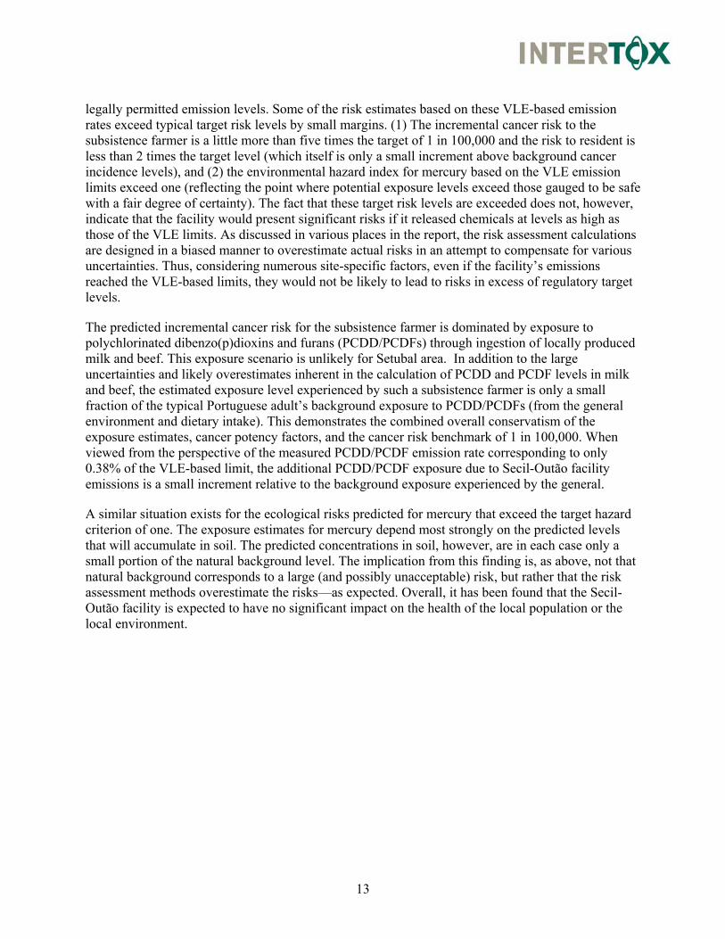


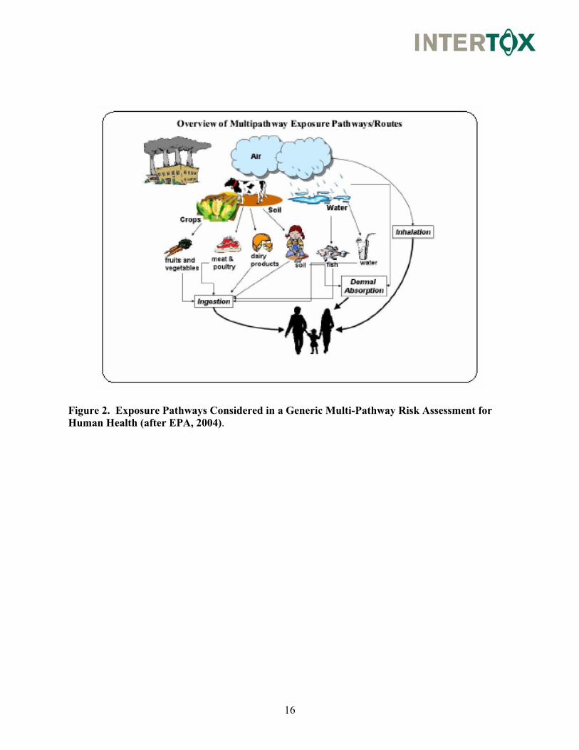
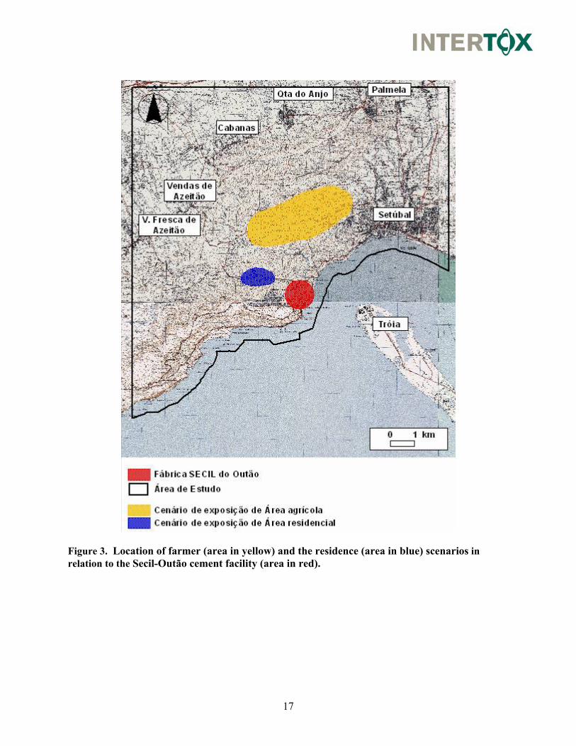
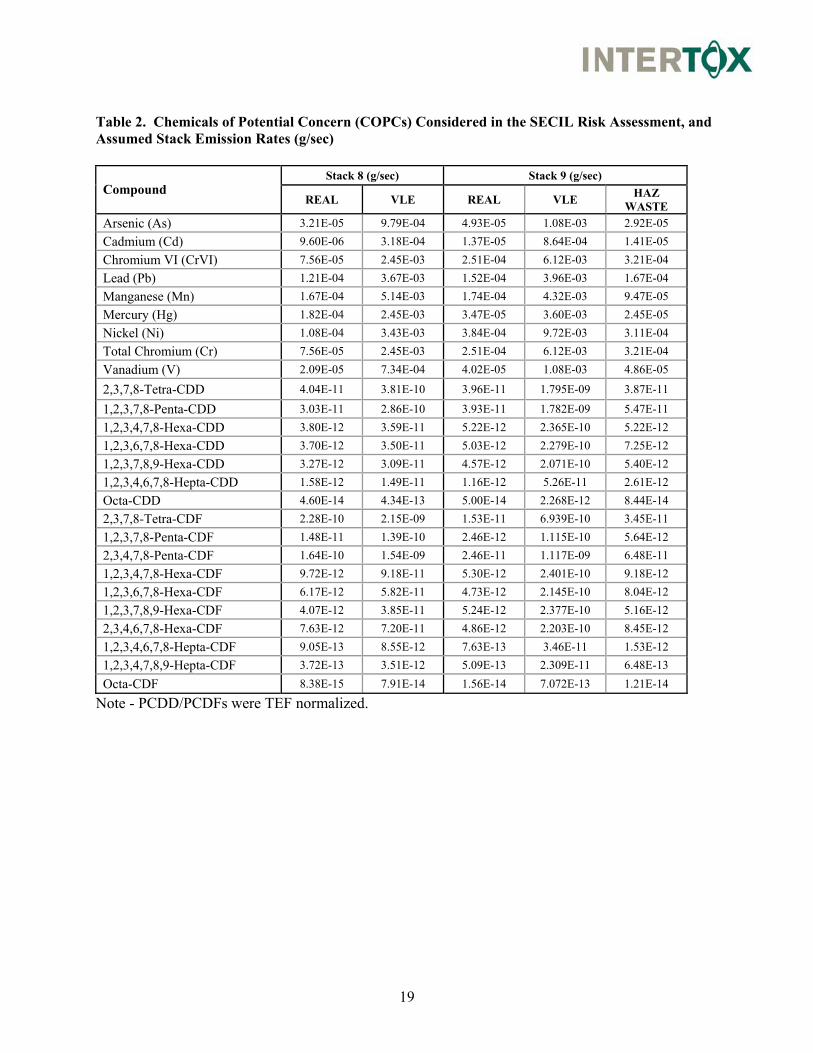
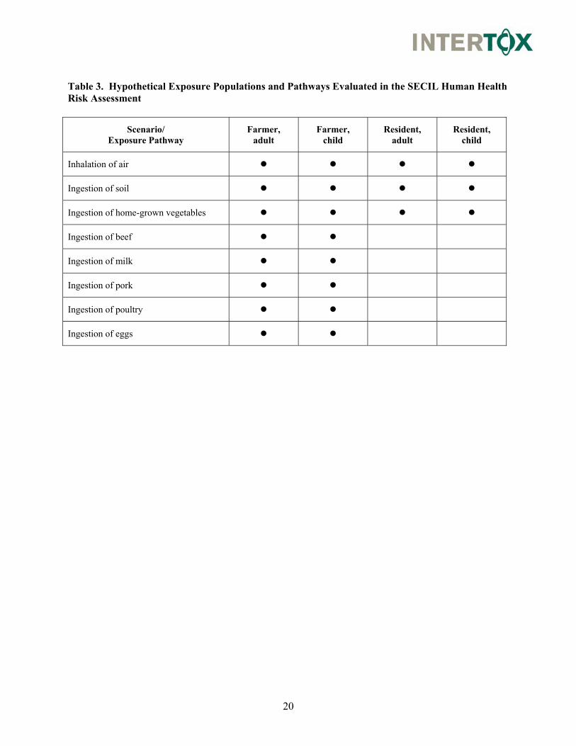
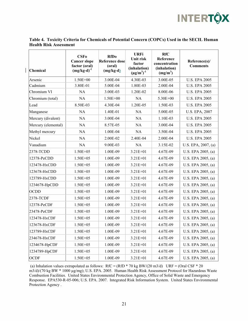

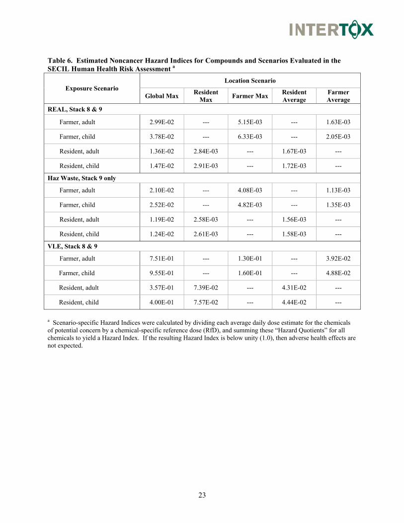
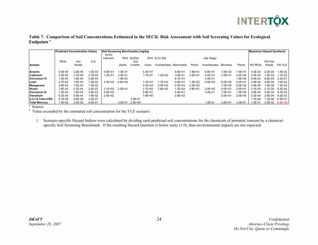


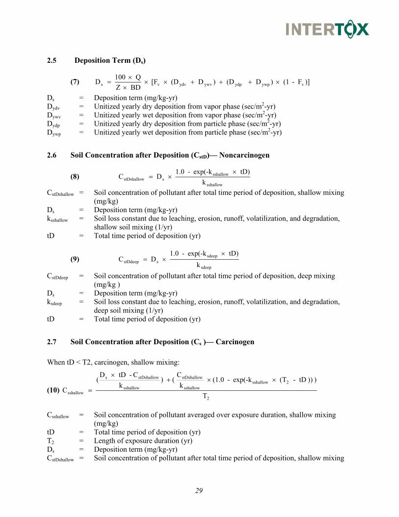
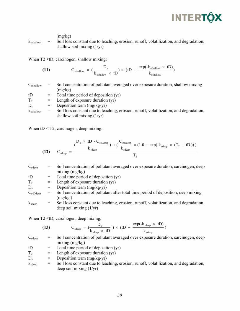

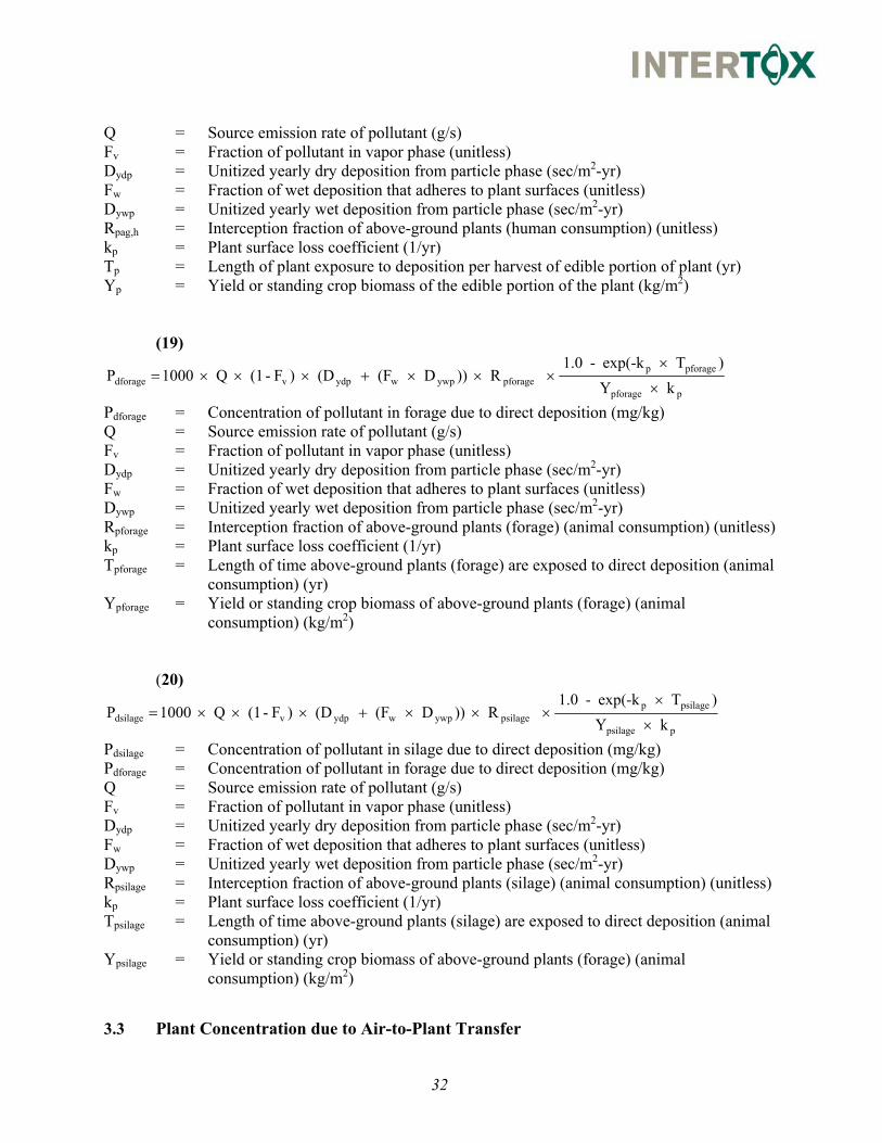


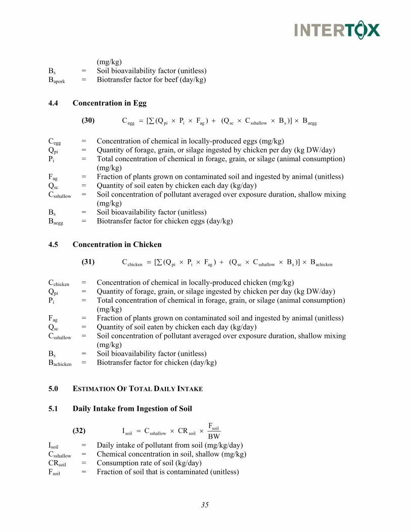
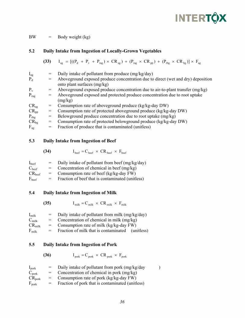
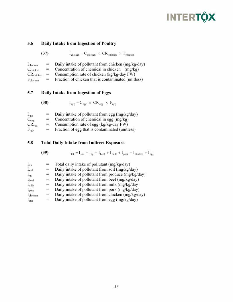

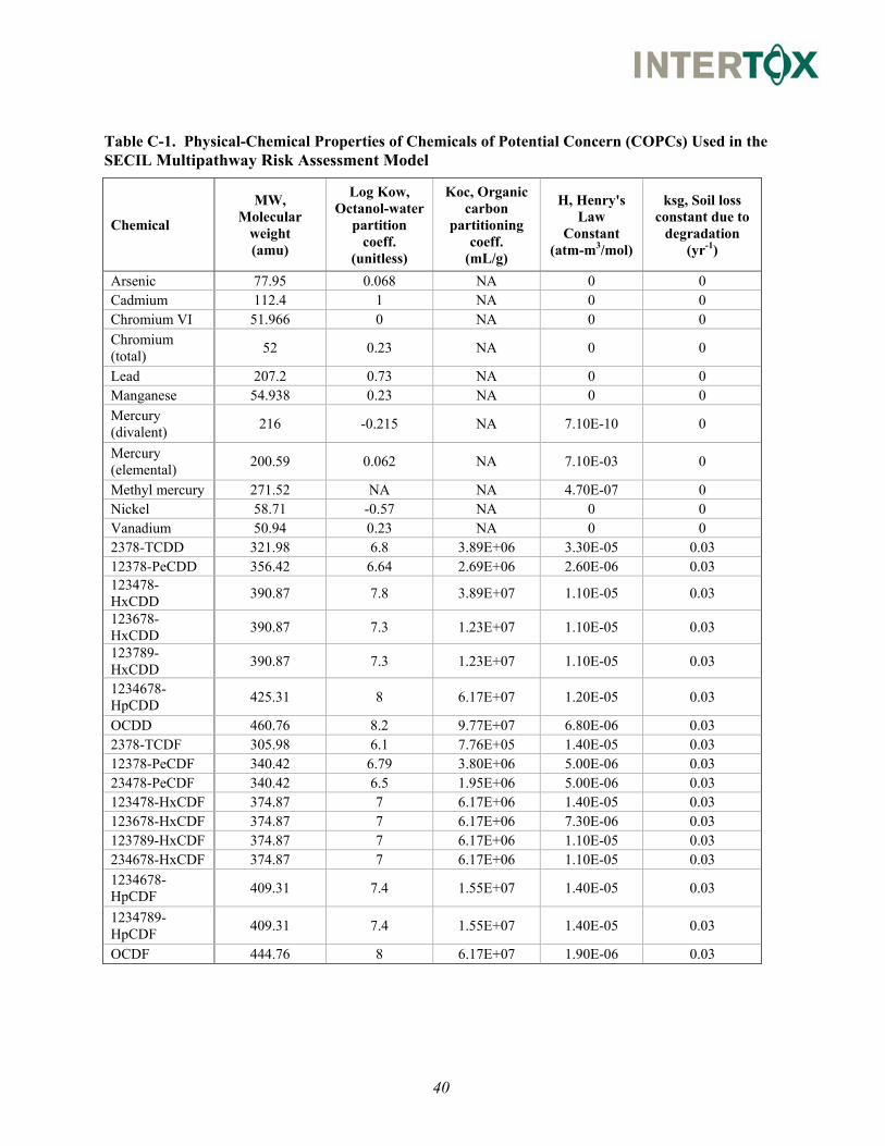

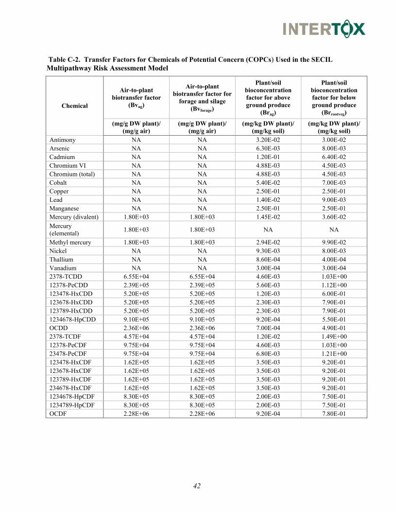
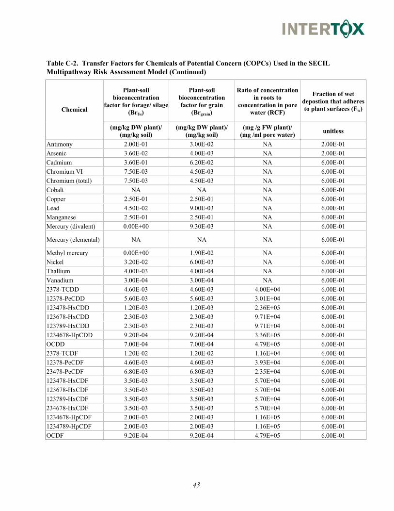

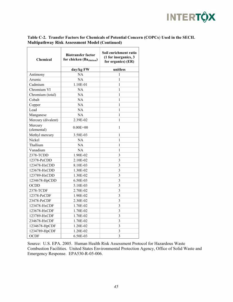


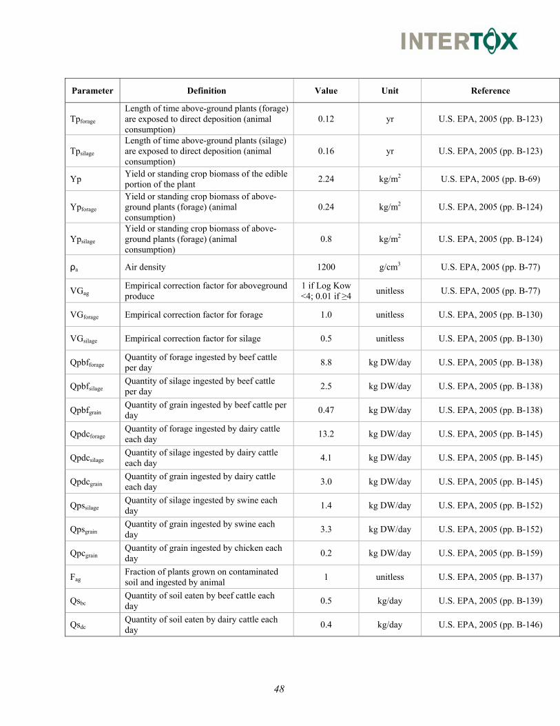


![RISK ASSESSMENT [ASSESSMENT]](https://static.documents.pub/doc/80x56/6212412fca52115ed803cf10/risk-assessment-assessment.jpg)


