Page 1
Risk Based Integrity Modeling of Offshore Process Component
Piping
by
Thevi A/P Sreetharan
14865
Dissertation submitted in partial fulfilment of
the requirements for the
Bachelor of Engineering (Hons)
(Mechanical Engineering)
FYP II JAN 2015
Universiti Teknologi PETRONAS,
Bandar Seri Iskandar,
31750 Tronoh,
Perak Darul Ridzuan,
Malaysia.
Page 2
i
CERTIFICATION OF APPROVAL
Risk Based Integrity Modeling of Offshore Process Component - Piping
by
Thevi Sreetharan
14865
A project dissertation submitted to the
Mechanical Engineering Programme
Universiti Teknologi PETRONAS
in partial fulfilment of the requirement for the
BACHELOR OF ENGINEERING (Hons)
(MECHANICAL)
Approved by,
_______________________________________________
(Dr. Tadimalla Varaha Venkata Lakshmi Narasimha Rao)
UNIVERSITI TEKNOLOGI PETRONAS
TRONOH, PERAK
January 2015
Page 3
ii
CERTIFICATION OF ORIGINALITY
This is to certify that I am responsible for the work submitted in this project, that the
original work is my own except as specified in the references and
acknowledgements, and that the original work contained herein have not been
undertaken or done by unspecified sources or persons.
_____________________
(THEVI SREETHARAN)
Page 4
iii
ABSTRACT
This paper discusses on the methodology to develop a risk-based integrity model of
offshore process piping (surface flowlines) which degrades due to corrosion. Gas
processing plants are highly hazardous which deals with chemicals at extreme
conditions such as high temperature and high pressure. These facilities should be
going through the right maintenance and inspection from time to time to ensure a
safe environment, continuous and fault-free operation. Deterioration of gas facilities
gives a major impact on the continuous operation of the facilities. This paper
proposes a risk-based integrity modelling methodology to have a fault-free operation
for the facility’s piping (also known as surface flowlines). The risk‐based integrity
model is to develop the model of offshore surface flowlines’ corrosion mechanism
efficiently to obtain an optimum replacement plan. The economic consequences of
offshore surface flowlines corrosion mechanism are developed in terms of the cost of
failure, inspection and maintenance. The optimal replacement strategy is obtained by
combining the collective posterior probability of failure and the corresponding rate of
corrosion. Risk-based integrity’s assessments use the structural corrosion data which
are modelled using the prior probability information. This prior probability
information can be restructured to posterior probability using Bayesian Theorem and
ASME B31.3 prediction method with the support of the inspection data of the
facility. Posterior probability will then be used to estimate the likelihood of the
piping failures in the facility. This can then lead to quantify the possible ageing
hazards to the facility and identify the replacement interval of the components to
avoid hazards. The consequence will be measured by cost as a function of time. This
paper focuses mainly on general corrosion on the surface flowlines (topside
pipeline).
Page 5
iv
ACKNOWLEDGEMENT
I would like to express my sincere gratitude to Dr.Tadimala V.V.L.N. Rao, my FYP
supervisor, for his guidance, enthusiastic encouragement and useful critiques of this
project. I would also like to express my very boundless appreciation to
Mr.Vevageran Velayutham, the Operation Engineer, Mr.Regukumaran Baskaran,
Senior Engineer of Integrity and Management and Mr.Mohammad Samsul Zairul,
the Reliability Engineer from Carigali Hess Operating Company, for their productive
time and willingness to give their assistance so generously by enabling me to visit
their offices to understand the concept and helping me in collecting the plant data. I
would also like to extend my appreciation and thanks to my dearest family for their
support and encouragement throughout my study.
Page 6
v
TABLE OF CONTENTS
Certification of Approval .............................................................................................. i
Certification of Originality ........................................................................................... ii
Abstract ....................................................................................................................... iii
Acknowledgement....................................................................................................... iv
List of Figures ............................................................................................................ vii
List of Tables............................................................................................................. viii
Abbreviations and Nomenclatures .............................................................................. ix
Chapter 1 Introduction ................................................................................................. 1
1.1 Background ................................................................................................... 1
1.2 Problem statement ......................................................................................... 2
1.3 Objective ....................................................................................................... 2
1.4 Scope of study ............................................................................................... 2
Chapter 2 Literature Review ........................................................................................ 3
2.1 Carbon Dioxide, CO2, Effect on Corrosion .................................................. 3
2.2 Corrosion Type: General or Uniform Corrosion ........................................... 4
2.3 Bayes’ Theorem ............................................................................................ 5
2.4 Risk-Based Integrity Modeling (RBIM) ....................................................... 6
2.5 Prior Probability Modeling ............................................................................ 7
2.6 Estimation of Likelihood Probability ............................................................ 7
2.7 Posterior Probability Modeling ..................................................................... 8
2.8 Economic Consequences analysis ................................................................. 8
Chapter 3 Methodology/Project work ........................................................................ 10
3.1 Bayesian Theorem Model ............................................................................ 12
3.1.1 Pressure Design Thickness of Process Piping .................................. 12
3.2 Economic Consequences analysis ................................................................ 13
3.2.1 Economic consequences of failure…………………………………13
3.2.2 Economic consequence of inspection……………………………...14
Page 7
vi
3.2.3 Economic consequences of maintenance……………………………...15
3.3 Tools Required .............................................................................................. 17
3.4 Gantt Chart and Key Milestone..................................................................... 18
Chapter 4 Results and Discussion .............................................................................. 20
Chapter 5 Conclusion and Recommendation ............................................................. 25
References .................................................................................................................. 27
APPENDIX I. Tools Used for Project Completion ............................................... 29
APPENDIX II. ASME B31.3 Calculation ............................................................. 30
Page 8
vii
LIST OF FIGURES
Figure 1: Weibull distribution analysis for corrosion .................................................. 5
Figure 2: Average inspection (cost/year) for corrosion degradation on pipeline......... 9
Figure 3: Sample of economic analysis ....................................................................... 9
Figure 4: Flow chart of the activities ......................................................................... 10
Figure 5: Economic consequence analysis chart ....................................................... 13
Figure 6: Gantt Chart of FYP 1 .................................................................................. 18
Figure 7: Gantt Chart of FYP 2 .................................................................................. 19
Figure 8: Prior and posterior probability density distribution for corrosion
degradation in the piping. ........................................................................................... 21
Figure 9: Average corrosion rate for corrosion degradation mechanism ................... 22
Figure 10: Total risk cost caused by corrosion for every year ................................... 23
Figure 11: Service period compare to corrosion cost................................................. 23
Page 9
viii
LIST OF TABLES
Table 1 : Data obtained for the simulation process .................................................... 20
Table 2: Results Obtained from Calculation above ................................................... 21
Table 3: Tools used to complete this project. ............................................................ 29
Page 10
ix
ABBREVIATIONS AND NOMENCLATURES
ABRREVIATIONS MEANING
RBIM Risk-Based Integrity Modeling
FYP I Final Year Project (Semester 1)
FYP II Final Year Project (Semester 2)
ASME American Society of Mechanical Engineers
PoF Probability of Failure
HSE Health Safety and Environment
CS Carbon Steel
CAPEX Capital Expenditure
OPEX Operational Expenditure
NDT Non-destructive test
RBI Risk based integrity
USD United States Dollar
MATLAB Matrix Laboratory Software
AEC Annual Equivalent Cost
Page 11
1
CHAPTER 1
INTRODUCTION
1.1 Background
Maintenance in terms of engineering is defined as the optimization of equipment,
procedures, and departmental budgets to achieve better maintainability, reliability,
and availability of equipment, where it can perform a requisite function (Thodi et al.
2009). Reputable maintenance should be steered to lessen the production hazards
and maintenance methodology such as Reliability Centred-Maintenance, Condition-
Based Maintenance and Total Productive Maintenance. These maintenance methods
can only be used based on the component’s Probability of Failure (PoF) where the
approaches will turn out to be more useful with the data about the failure discovery,
component, repair, budgets, maintenance plan and management policies (Khan et al.
2006). While the consequences of failure, inspection and maintenance is not
applicable through these maintenance strategies.
Risk-based Integrity Modeling has become a very valuable method and a recognized
tool based on the life-cycle risks in enhancing the maintenance activities.
(Saharuddin et al. 2011) mentioned that the selection of a risk analysis method has a
key effect on the identification of risk causes and in developing a true (Backlund,
2002) decision making in maintenance process. Cautious requirement identification
and an efficient method with proper goals are required while performing risk
analysis. Gerhardus (2012) has stated that integrity maintenance of offshore process
piping lines has been a subject of exploration for many years, yet needed to be
justified. This paper discusses about the importance of Risk-Based Integrity to
measure the risk posed by the offshore surface flowlines.
Page 12
2
1.2 Problem statement
Offshore process components reducing its life span earlier than predicted durability.
This is because the facility is going through high failure rate due to improper
replacement strategy, which causes relatively high unplanned maintenance cost due
to unexpected failures. Ensuring continuous and failure free operations of offshore
components such as pipeline is paramount, taking into account the production
deferment and additional cost incurred due to unplanned maintenance activities.
There is a great need to avoid this situation from stirring and to minimize the
environmental and cost impact. To ensure a fault-free operation throughout the assets
life, a risk‐based integrity model (RBIM) can be used to obtain an optimal
replacement strategy for the corrosion of the surface piping. This model will be
developed in terms of the cost of failure, inspection and maintenance.
1.3 Objective
The purpose of this paper is about the importance of Risk-Based Integrity, which is:
To measure the risk posed by corrosion in offshore piping (only surface lines)
To develop a risk‐based integrity model for the optimal replacement of
offshore process piping.
To develop the failure consequences of offshore process piping corrosion in
terms of the cost of failure, inspection and maintenance.
1.4 Scope of study
The scope of this study will be focusing on the topside surface flowlines downstream
of separator at offshore process facility. The scope of this project is within the
offshore gas processing facility, focusing on carbon dioxide system of the facilities,
study will be on corrosion of the piping in the facility. The study of the thesis is
confined to develop a risk‐based integrity model for the optimal replacement of
offshore process piping. Throughout the study failure consequences of the piping
corrosion are developed in terms of the cost of failure, inspection and maintenance.
This study will measure the combination of collective posterior PoF and the
corresponding cost of corrosion for an optimum replacement strategy. This study
also will show that in order to develop RBIM, Bayesian theorem model and
corrosion rate prediction method in ASME B31.3 are used.
Page 13
3
CHAPTER 2
LITERATURE REVIEW
This paragraph represents literature review on the areas related to the Risk-Based
Integrity Modeling (RBIM). There has been an issue of research going on for
voluminous years regarding the integrated maintenance of the process components
because lack of maintenance will cause deterioration of assets where it has a very
critical effect on the operation of gas processing platforms (Kallen, 2002). Assets are
subjected to corrosion which will eventually degrade (Straub, 2004).
RBI involves an optimal maintenance process (involves cost) which will be used to
test the corrosion of equipment or components in industrial plants. Health, Safety and
Environment (HSE) and risk of business will be examined by ranking failure
probability and consequence through the RBI assessment. Maintaining the integrity
of offshore process facility is a prime concern for the oil and gas industries in the
world. An optimal methodology is necessary to avoid any failure consequences from
occurring.
2.1 Carbon Dioxide, CO2, Effect on Corrosion
Carbon dioxide is an acidic oxide (covalent compound) and it reacts with water
which will result in carbonic acid. CO2 corrosion is also known as “sweet corrosion”
(Barker et al, 2013). Majority oil and gas industry is facing failures due to CO2
corrosion on carbon steel (CS) and has lack of knowledge to overcome this problem.
Kermani et al. (2003) has commented that CO2 corrosion is the most widespread type
of risk faced by oil and gas sector. In search for more oil and gas source, the
Page 14
4
operational activities have moved to a deeper and high risk environment, thus, it is
moving to a higher pressure and higher temperature condition. These have evolved
to more challenges faced by the industry, where the project development and the
operation cost is also increasing. In addition, there will be needs to identify the
facilities integrity and accurate estimation of materials performance to avoid major
failures and risk. The effect of corrosion in this industry can be observed in terms of
CAPEX and OPEX, and HSE (Kermani, 2003).
2.2 Corrosion Type: General or Uniform Corrosion
General corrosion is common among CS. General Corrosion focuses on surface of
the pipe and easily estimated by good inspection because of its uniform rate of
corrosion. There is always excess material thickness will be provided to allow the
corrosion to thin the material to a certain allowable amount of minimum thickness
(based on ASME B31.3, 2011); if it falls below the minimum allowable thickness,
the pipe will start to leak and eventually will fail. Thus, brings risk to the safety of
the surrounding.
General corrosion is also known as uniform corrosion, which occurs moderately and
evenly distributed over the surface, leading to a relatively uniform thickness
reduction (Cicek, 2009). It is the most common form of corrosion and responsible
for most of the material loss. Prediction test of thickness reduction (corrosion rate)
for this form of corrosion is simple with availability of proper inspection data
(Winston, 2007). This also will lead to the prediction of probability of failure (PoF),
and life expectancy of the product.
Winston (2007) has mentioned that there are two fundamental criteria must be
considered to determine the PoF, which are:
The form of corrosion and the corrosion rates.
The possible effectiveness of corrosion inspection and monitoring.
Page 15
5
Figure 1: Weibull distribution analysis for corrosion
Figure 2 refers to the Weibull distribution plot which was obtained by (Thodi et. al,
2013). This is the posterior samples and was used to estimate their parameters of
risk. This is then lead to the prediction of failure time of the piping.
2.3 Bayes’ Theorem
Reliability engineering measure the failure due corrosion which can be observed for
a period of time before the failure happens (Park & Padgett, 2006). Thodi et al.
(2009, 2010) has discussed about estimating the probability of structural
deterioration-related failure, which can be related to the present condition of the
component. Corrosion standards and failure observations data reflect when
conducting inference on the statistical factors of the components’ lifespan
distribution. Rate of failure is determined through the NDT data and the
professional’s knowledge and can be obtained during the inspection. NDT data can
be used to derive the likelihood probability. Based on the data collected from the
facility, inspection and piping lines, Bayesian theorem model and ASME B31.3
prediction analysis will be used to model the system.
Prior probability will be a part of the research where it is studied through judgmental
and by analyzing the standard database. The simulation-based Metropolis-Hastings
(M-H) algorithm method was used to make estimation on the posterior models
because the prior-likelihood combinations were non-related to each other (Khan et al.
2006). Posterior model must be developed for the corrosion in piping.
Page 16
6
Conditional probability of an event is known as a probability achieved with
additional data that some other event has already occurred (Mario,n.d.). Bayes’
theorem deals with sequential events, whereby new data is obtained for a subsequent
event. The new data that was obtained will be used to revise the probability of the
initial event.
Prior probability and posterior probability models are used commonly in Bayes’
Theorem. Probability is a degree of acceptance of how far that it is true based on the
data obtained. According to Chienet al. (2009), these models are reliable to predict
the future failure probability of failing components in the process facility. As seen
from Figure 1, Bayesian uses population parameters which are associated with a
posterior probability which quantifies the degree of acceptance from the obtained
data [refer to Equation (1)].
2.4 Risk-Based Integrity Modeling (RBIM)
The primary concern in engineering field is to manage risk, reduce and abolish it to a
certain acceptable levels. Combination of the probability of a failure event and the
severity resulting from the failure is known as risk in engineering field. According to
Thodi et al. (2013) RBIM is a methodology to measure the risk to life modelled by
the deteriorating components and to mitigate that in an economical method.
Components will deteriorate if there’s any physical breakage, leaks, and
environmental effects. These deteriorations are stochastic processes. Therefore, the
main concept in RBIM is to do estimation of the probability of structural failures and
their consequences. Probability of failure is determined through stochastic modeling
of the corrosion (Selvik J.T. et al. 2011). Through Bayesian prior-posterior analysis,
the probability distribution function can be achieved, which can also be used to
model a realistic inspection data.
The failure occurrence, inspection and the maintenance tasks can be used to do the
consequence analysis which is focused on estimating the cost sustained (Khan et al.
2013) the consequence analysis is done to estimate the consequence of undesirable
failure occurrences in terms of the cost of failure, corrective maintenance and
Page 17
7
preventive maintenance. Failures can lead to perform replacement for the
components which will result in high cost corrective maintenance and unplanned
shutdown in oil and gas process component facilities. These will cause a very large
impact on maintenance tasks done and the cost to replace the component. Thus, an
organization needs an optimal policy which aims to avoid large replacement cost and
to minimize the total operating cost. According to Gerhardus (2012), the cost of
maintenance includes cost of attaining access to the site, cost of preparation before
inspection and maintenance and cost of detecting and sizing of defects using the non-
destructive tests (NDT), cost of conveyance of equipment and cost of qualified
technicians. Failure costs include breakdown loss, shutdown loss and environmental
damage and liability loss.
2.5 Prior Probability Modeling
A prior probability is an primary probability value initially obtained before any
additional information is received (Mario, n.d.). For any type of component
degradation, the prior probability refers to the initial knowledge about each type of
degradation processes. The corrosion data for the prior distribution can be obtained
by few methods, such as frequency graphs, by conducting statistical investigations
and plotting probability graphs. A rational agreement of results can be made by
analyzing the historic data of the same or the similar piping lines installations
(Congdon, 2006), even though the prior probability data is subjective.
2.6 Estimation of Likelihood Probability
Estimation of likelihood probability (Montgomery et al. 2002) is the process of
estimating the parameters of statictical models. This method selects the parameters
from the model which maximizes the likelihood function, and thus, it maximizes the
probability of the observed data under the resulting distributionwhich gives a unified
approach to estimation. Estimation theory is the division in statistics which deals by
estimating the values of parameters on measured data which has random element.
Estimation theory uses the measured data to approximate the unknown parameters.
Page 18
8
The failure rate of an undesirable event in RBI is called likelihood. American Bureau
of Shipping, ABS, (2003) has mentioned that likelihood is considered to be the most
important factor in the evaluating risk since it directly affects the selection of
inspection frequency. Pipe lines that has relatively high-risk will be prioritized
during the screening and more detailed analysis on corrosion and frequency will be
performed, e.g. NDT inspection data will be used to estimate the likelihood
probability of different time of corrosion processes.
2.7 Posterior Probability Modeling
Posterior probability is known as Bayesian statistics, where the model is treated as
another unknown parameter of a random event (also known as conditional
probability) that is done after the background condition is measured (Congdon,
2006). The word ‘posterior’ is defined as the condition that was taken into account
after obatining the relevant results related to the particular process which is being
measured. It is treated as a random variable from the evidence that was resulted from
the test done on the same or similar processes (ABS, 2003). A range of approximate
methods must be proposed in order to select the Bayesian model. After the
observation of data, Bayesian model is related to prior model probabilities and
posterior model probabilities. A M-H algorithm approximation needed to be used to
identify the posterior probability (Berger et al. n.d.).
2.8 Economic Consequences analysis
RBIM is done to minimize the risk level by preventing faliures caused by the
corrosion and thus will maximize the profit due to less risk and failure (Purnell,
1999). Consequences analysis is done to measure the risk level and consequences is
represented in USD unit because risk is evaluated as the expected loss of business
due to certain failures. Analysis of economic consequences is further explained.
Cost analysis of corrosion for inspections is built on posterior functions as shown in
Figure 2. Based on the corrosion analysis graph, it has a preventive replacement time
of approximately 14 years and failure period of 26 years approximately. There are 2
minimum point found on the corrosion cost analysis graph, one is at year 10 and
Page 19
9
another one at year 22 approximately. The pipeline studied in this research paper was
operating for 5 years and inspection was done for only once, then the next inspection
should be due in 5 years’ time. The minimum expected results for the replacement
period for this study will be around 10 years as well.
Figure 2: Average inspection (cost/year) for corrosion degradation on pipeline;
Courtesy of (Khan, 2006)
Figure 3 shows that the failure cost is decreasing over time. While the inspection and
maintenance cost is increasing over time during its service life. The increase for the
maintenance and inspection cost are assumed to occur due to the corrosion which
affects material strength of the pipeline.
Figure 3: Sample of economic analysis from (Thodi et al., 2013)
Page 20
10
CHAPTER 3
METHODOLOGY/PROJECT WORK
Figure 4: Flow chart of the activities
Model development:
Model piping failure using Bayesian
method. 1000 iteration in MATLAB to
develop the risk-based integrity model.
Start
Model validation:
⁻ Risk calculation
⁻ Estimate optimal inspection and
replacement intervals
⁻ Consequence analysis
Accepted
Report
Problem Statement:
Relatively high unplanned piping maintenance
cost due to unexpected failures of piping due to
corrosion
Data Gathering:
Identify possible degradation mechanism to
develop model by gathering degradation
parameters, and consequence analysis
parameters.
Determine failure probability using a posterior
probability model and previous inspection data
Data analysis of failure
consequences:
⁻ Economic consequence of
failure
⁻ Economic consequence of
inspection
⁻ Economic consequence of
maintenance
Yes
No
Page 21
11
Data analysis of failure consequences should be conducted to quantify the economic
impact on failures, inspection and maintenance before the RBIM is developed. The
analysis is crucial to validate the RBI model if it can maximize the profit and
minimize the risk by preventing failures associated with corrosion. The criteria of an
effective RBIM is to have the total cost of failure reduced after its implementation.
The results are valid if the Annual Equivalent Cost (AEC) is in a convex function as
shown in Figure 4 and if the replacement time of both results are approximately
equivalent (if valid the graph should be convex).
Page 22
12
3.1 Bayesian Theorem Model
Bayesian Theorem is evaluated through calculating posterior probability
distribution, , where , is prior probability, is the likelihood
function, [ (
) ] is the evidence (normalization constant useful for
Bayesian model selection)(Thodi et al., 2013).
(
)
(
)
(1)
Thodi et al. (2013) has proven that posterior density, , summarizes the whole
figures, after attaining the data and conveys a root for inference regarding the
corrosion parameters.
3.1.1 Pressure Design Thickness of Process Piping
Based on ASME B31.3, (2011), pressure design thickness in straight pipe under
internal pressure
(2)
Where pressure design thickness, t, is the product of internal design gage pressure, P
and outside diameter of pipe, D, divided by stress value for material, S, quality
factor, E, weld joint strength reduction factor, W, and coefficient, Y.
(3)
Where tm is the minimum require thickness including corrosion and mechanical
allowance, and c is the sum of the mechanical allowances.
Page 23
13
3.2 Economic Consequences analysis
(ABS, 2003; Thodi et al. 2013)
Figure 5: Economic consequence analysis chart
3.2.1 Economic consequences of failure
(Thodi et al. 2013)
3.2.1.1 Loss due to breakdown The is obtained from the
is given by (Crowl and Louvar, 2002), where
, , g , and
.
√ (4)
3.2.1.2 Cost of breakdown due to corrosion, Clc is measured by multiplying the
average number of critical failures in the piping, Ecf, failure and loss of
commodity probability, Pofl, the duration of the commodity loss, Tcl, quantity
of commodity loss, Qcl, and cost of downtime, Cdt.
(5)
3.2.1.3 Cost of shutdown due to degradation (USD), , is measured using the
Consequence of failure
1. Economic consequences of failure
2. Economic consequences of inspection
3. Economic consequences of maintenance
Degradation failure
Page 24
14
shutdown cost, multiplied with unit cost of product (USD/barrel), , and
total delay of maintenance (days), .
(6)
3.2.1.4 Cost of spill clean-up due to corrosion,Csc is measured by multiplying loss of
product, Qp, duration of spillage, Tds,and cost of spill cleanup, Cscs.
(7)
3.2.1.5 Cost of damage in nature due to corrosion, , is the product of the
multiplication of the discharge of product due to degradation (ton/hour),
and the duration of discharge (hour), .
(8)
3.2.1.6 Total cost due to corrosion failure
(9)
3.2.2 Economic consequence of inspection
(Thodi et al. 2013)
The cost of inspection for degradation calculations are:
3.2.2.1 Cost to gain access for corrosion inspection, , is calculated by
multiplying the cost of inspection technician per hour, , with total duration
of work done to inspect, .
(10)
3.2.2.2 Cost of the preparation to inspect, , is the product of multiplication of
cost of inspection labour per hour, , with the duration of work done to
prepare for inspection (surface preparation) (hours) .
(11)
3.2.2.3 Inspection technician cost. This cost is measured by defining which type of
inspection is done to inspect the piping and how many personnel is involved
for how long (t), which involves the cost of:
Visual and radiographic inspection of piping, (12)
Page 25
15
UT piping (thickness and defect), (13)
3.2.2.4 Technical expert, (14)
stands for technical expert consultancy fees (calculated hourly)
3.2.2.5 Logistics, (15)
stands for cost of consumables, is the cost of equipment for
inspection, and is the cost for storage and transportation done during
inspection.
3.2.2.6 Total inspection cost involved to inspect the corrosion of piping is:
(16)
3.2.3 Economic consequences of maintenance
(Thodi et al. 2013)
Few categories are considered to measure the cost of maintenance for corrosion,
which are:
3.2.3.1 Cost to gain access for corrosion maintenance, , is calculated by
multiplying the cost of inspection technician per hour, , with total
duration of work done to inspect, .
(17)
3.2.3.2 Cost of the preparation to inspect, , is the product of multiplication of
cost of expert labour per hour, , with the duration of work done to prepare
for inspection (surface preparation) (hours) .
(18)
3.2.3.3 Maintenance technician cost. This cost is measured by defining which type of
maintenance is done to inspect the pipelines and how many personnel is
involved for the period of time involved to do maintenance, t.
Gauging defects personnel cost, (19)
Logistics cost,
Page 26
16
Total cost of gauging defects for corrosion maintenance,
(20)
3.2.3.4 Reparation process cost for corroded piping:
Repair, (21)
Weld quality test and coating restoration, (22)
stands for cost of weld quality test personnel (calculated hourly)
Technical assistance, (23)
Other minor repair, (24)
stands for cost of parts or spare and consists of cost of
consumables.
3.2.3.5 Total maintenance cost of corrosion degradation,
(25)
Annual equivalent cost (AEC) due to corrosion failure, inspection and maintenance,
will be calculated for the service period of total years, n, by using annual worth,
present worth analysis with an annual interest rate of i percent.
Page 27
17
3.3 Tools Required
Throughout the project, several tools will be used to compile and analyze relevant
data. The tools required during the project consist of the following software’s as
shown in the table in APPENDIX I.
Page 28
18
3.4 Gantt Chart and Key Milestone
FYP I
No Activity Week
1 2 3 4 5 6 7 8 9 10 11 12 13 14
1.0 Selection of project topic
2.0 Preliminary research work
2.1 Literature review
2.1.1 Obtain equations and probability distributions
2.1.2 Methodology
3.0 Submission of extended proposal
4.0 Design of experiment
4.1 Identifying component that is affected with
degradation
4.2 Selection of degradation processes
4.3 Identifying & obtaining standards and parameters
needed
5.0 Proposal defence
6.0 Project work
6.1 Measure and test the probability distribution models
7.0 Submission of interim draft report
8.0 Submission of interim report
Figure 6: Gantt chart of FYP I
Page 29
19
FYP II
No Activity Week
1 2 3 4 5 6 7 8 9 10 11 12 13 14 15
1.0 Project work
1.1 Data compilation and consequence analysis measurement
2.0 Submission of progress report
3.0 Data analysis and discussion
3.1 Tabulation of data and develop model
3.2 Review of data ( discussion of results obtained)
4.0 Pre-SEDEX
5.0 Submission of draft of final report
6.0 Submission of dissertation (soft bound)
7.0 Submission of technical paper
8.0 Viva
9.0 Submission of project dissertation (hard bound)
Figure 7: Gantt chart of FYP II
Page 30
20
CHAPTER 4
RESULTS AND DISCUSSION
Offshore component that was selected in this study are gas surface lines. Table 1 below is
the case study of this project which was obtained from a gas processing company.
Table 1 : Data obtained for the simulation process Design Parameters Separator Pipeline
Design temperature 140˚F/-20˚F
Design pressure 840 Psig
Operating temperature 99 ˚F
Operating pressure 730 Psig
Pipe dimensions Diameter = 24in
Wall thickness = 22.61mm
Material of construction Carbon steel
Active damage mechanism
for pipeline
corrosion, erosion, cracking
due to stress
Other Parameters Values
Tensile strength 90 MPa (min)
Yield strength 50 MPa (min)
Inspection cost RM5,000
Preventive replacement cost RM100,000
Failure cost RM500,000
These data was used to resolve to get the replacement interval of the piping by doing
simulation in MATLAB software to obtain the Risk-Based Integrity Model.
This project involves CS piping segment of 24 inch diameter with the wall thickness of
35.61 mm. This research is done based on a straight piping with the length of 200 m after
the separator. This pipe is used to illustrate the Bayesian Theorem model to get the
replacement interval of the piping. Based on Figure 8, the peaks of prior and posterior
probability density distribution are very much attached to each other. Both the functions
are evenly spread in the figure below. Peak of posterior probability distribution functions
are at 0.14 mm/year, while for prior probability distribution is at 0.12 mm/year. Prior
Page 31
21
density distribution is based on real time data, which is obtained from inspection data.
The posterior density distribution is simulated and estimated based on the information
obtained from prior density distribution. This density distribution functions will assist to
obtain the Bayesian Theorem model’s wall thickness prediction.
Figure 8: Prior and posterior probability density distribution for corrosion degradation in
the piping.
Table 2: Results obtained from calculation based on ASME B31.3
Unit Results obtain
Internal design gage pressure, P 840 psig
Outside diameter of pipe, D 24 inch
Stress, S 90 ksi
Quality factor, E 1
Weld joint strength reduction factor, W 1
Coefficient, Y 0.4
Sum of the mechanical allowances, c 0.2
Pressure design thickness, t 23.66 mm
Minimum allowable thickness, tm 24.16 mm
Difference in t 9.09 mm
Number of years pipe operated 11 years
Corrosion rate 0.8263 mm/year
0
1
2
3
4
5
6
7
0 0.1 0.2 0.3 0.4 0.5 0.6 0.7 0.8
Den
sity
Corrosion rate (mm/year)
Density distribution
Prior probability
Posteriorprobability
Page 32
22
1
6
11
16
21
26
31
36
41
0 5 10 15 20 25 30 35 40 45
Thic
knes
s (m
m)
Year
Pipe wall thickness
Figure 9: Average corrosion rate for corrosion degradation mechanism
Figure 9 is consists of 2 main graphs, which are the prediction of wall thickness by using
ASME B31.3 and the prediction of wall thickness by using Bayesian Theorem model.
ASME B31.3 wall thickness prediction is widely used in oil and gas industry to predict
the failure period of pipe by measuring the internal pressure design of the pipe and the
wall thickness. This paper is comparing the Bayesian Theorem wall thickness prediction
with ASME B31.3. The pipe would fail when the predicted wall thickness lines interferes
with the minimum allowable thickness line which is 24.16 mm. Thus, the piping failure
period predicted by using ASME B31.3 is at the midyear of 16 (16.5 years)[the
calculation method is shown in APPENDIX II], while the failure period predicted using
the Bayesian Theorem is at the end of year 14 (14.8 years). The optimal replacement
interval is the interval which corresponds to minimum risk, thus, taking into account the
minimum risk, based on Figure 9, the replacement interval should be before year 14
(Thodi et al., 2013). The Bayesian Theorem graph was obtained by performing 1000
iteration run in MATLAB software.
Page 33
23
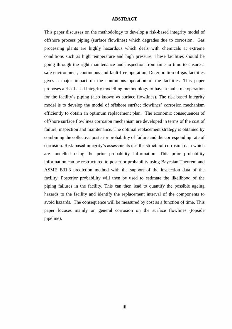
Figure 10: Total risk cost caused by corrosion for every year
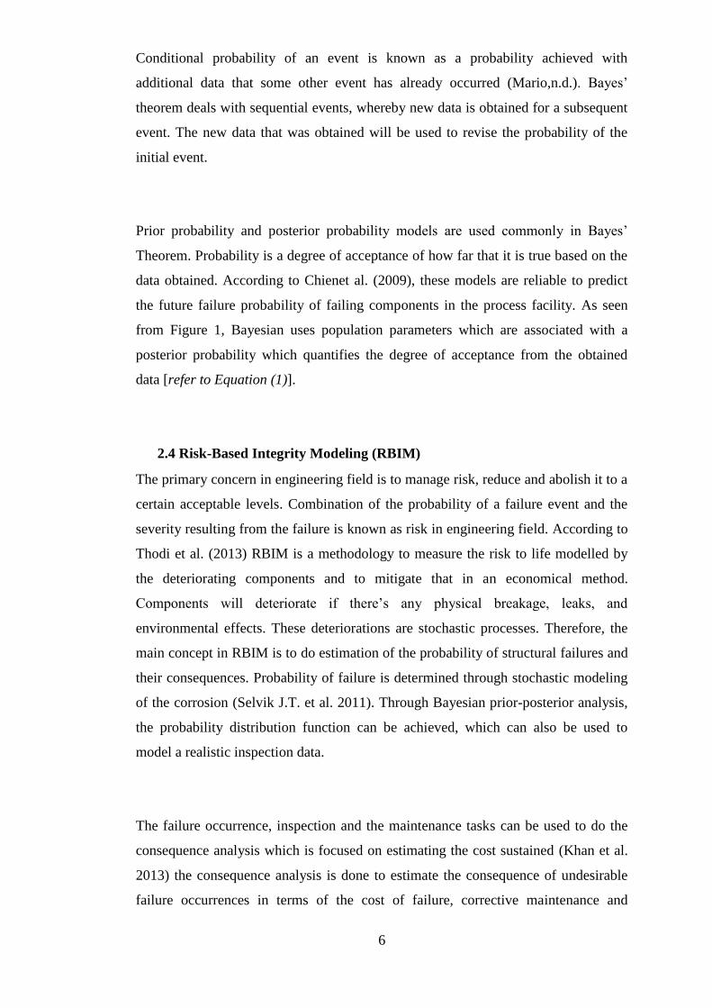
Figure 11: Service period compare to corrosion cost
Cost of risk due to corrosion was calculated and the results are shown in Figure 10 and
Figure 11. Figure 10 only shows the overall risk cost for the corrosion degradation
process by performing economic consequence analysis for the Annual Equivalent Cost
(AEC). An opaque trend is achieved for the cost of the functioning lifecycle risk due to
corrosion in the form of a partial convex curve. An irregular convex line curve is found
0.00
100,000.00
200,000.00
300,000.00
400,000.00
500,000.00
600,000.00
700,000.00
800,000.00
900,000.00
0 5 10 15 20 25 30 35
Co
st (
$)
Years of service
Risk Curve: Annual Equivalent Cost
RiskCurve
0
100000
200000
300000
400000
500000
600000
700000
800000
0 5 10 15 20 25 30
Co
sts
($)
Years of service
Service period v. cost of corrosion
AEC (Total)
Failure cost
Inspection cost
Maintenance cost
Latest inspection done
Page 34
24
until year 11 because the line is based on the actual data and rate acquired from few
inspections done to the piping. After year 11, it shows a gradual and regular increase in
the cost, this is due to the failure risk caused by corrosion to the piping.
Figure 11 shows the AEC and the estimated breakdown cost, which is divided into annual
equivalent failure, maintenance, and inspection cost. Failure, inspection and maintenance
cost analysis graph are obtained from the economic cost analysis that was done by
assuming a fixed rate of annual interest rate of 10.47%. Figure 11 is the comparison
between the failure, inspection, maintenance and the AEC analysis done. Present worth
factor was used to obtain the maintenance and inspection cost estimation by assuming the
same rate of interest. The AEC is observed to be reducing for the first three years, at the
fourth year, it started to increase and reduce mildly, and there is a significant fall at year
12 (lowest peak), and a sudden rise in cost at year 14. The same goes with the annual
equivalent of failure cost, the significant increase in the failure cost after year 13 is due to
the corrosion risk. This proves the results which were obtained by (Thodi et al., 2013),
the escalation in inspection and maintenance costs are due to the loss caused by the
deterioration of the material strength of the flowlines. The optimal replacement interval
based on Figure 11 is at year 12, which is the minimum cost observed and it is the cost
efficient point of replacement interval, where there will be less expenditure compare to
the other years. The calculated AEC is identified to be a distorted and partial service life
convex curve function.
The ideal optimal replacement interval strategy is between year 12 to year 13. This is due
to the consideration of the minimum risk and minimum cost which determines the ideal
optimal replacement interval. This decision was made by comparing the results obtained
in Figure 9 and Figure 11.
Page 35
25
CHAPTER 5
CONCLUSION AND RECOMMENDATION
Risk posed by corrosion in piping is measured in terms of failure rate and cost. The
failure rate predicted based on Bayesian Theorem is at year 14.8. The cost due to
corrosion is increasing by time because the material is degrading and losing its strength.
One of the advantage of the RBIM strategy is, the probability density distribution
function for the corrosion can be updated using the same Bayesian Theorem method. This
enables the failure rates easy to be modified when the actual measurements are available
after the inspections are done in the upcoming years. Results obtained for this case study
illustrates that this method used in this project yields a valid judgment for the
replacement interval that was achieved. The optimal replacement interval is the period or
meantime of which resembles to the minimum risk and minimum cost. Implementation of
replacement at this interval will reduce the operation’s risk level locked to the ALARP
level. This study focused on a straight piping (surface flowlines) segment which was
affected by the carbon dioxide corrosion degradation. Decision to replace the surface line
is more effective than carrying out maintenance. Optimal replacement is to return the
lines to a more integrated condition which possess less risk compare to the ones that have
operated for very long period.
Risk-based Integrity Model is developed by using Bayesian Theorem to find the optimal
replacement strategy of the piping by knowing the time to replace the piping before it
enters the failure point. The optimal replacement interval is ideal when it corresponds to
the minimum risk (safety and cost is considered). In conclusion, the replacement
intervals, which is known as the method of the RBIM strategy was discussed. The ideal
optimal replacement interval of this case study is at year 12, given that it is the most cost
effective and safer period before it reaches the failure point. Replacement strategies are
focused to cure the consequences of the deterioration of the component. It also act as a
remedy on strength loss and outmodedness of the process components, in this case is
piping (flowlines). The component deterioration makes the component to face reduction
Page 36
26
in the efficiency of the operation, thinning of the wall thickness and reduction in the
material strength. Outmodedness take place as an outcome of new technology
advancement is introduced in the industry.
The failure consequences of offshore process piping corrosion are identified in terms of
Annual Equivalent Cost (AEC) (also known as overall cost). The overall cost is obtained
by adding the failure, maintenance, and inspection cost together. Cost will escalate if the
component degrades over time and if it fails. To avoid the failure, Risk-based Integrity
Model is done by identifying the replacement interval. Initially, the corrosion cause was
discussed, followed by a brief discussion on the RBIM, Bayesian Theorem model.
Further discussed about the economic consequences analysis, where the AEC is
calculated by combining the failure, maintenance and inspection costs. The density
distribution of the piping corrosion is then combined with the economic analysis to
produce the effective life expectancy risk curve (Bayesian model), which is also known
as RBIM.
Page 37
27
REFERENCES
American Bureau of Shipping (ABS), A.-B. o. S. (2003). ABS Surveys using RBI for the
offshore industry (pp. 18-19). 16855 Northchase Drive, Houston, TX 77060 USA
Act of Legislature of the State of New York 1862
AISI, A. I. S. I. (2011). Steels.
ASME. (2011). Process Piping ASME Code for Pressure Piping, B31: THE AMERICAN
SOCIETY OF MECHANICAL ENGINEERS.
Backlund, F. a. H., J. (2002). Can we make maintenance decisions on risk analysis.
Journal of Quality in Maintenance Engineering, 8(1), pp. 77-91.
Barker, R., Hu, X., Neville, A., & Cushnaghan, S. (2013). Inhibition of Flow-Induced
Corrosion and Erosion-Corrosion for Carbon Steel Pipe Work from an Offshore
Oil and Gas Facility. CORROSION ENGINEERING SECTION, 69(2).
Cicek, V., & Al-Numan, B. (2009). Corrosion Chemistry. 3 Winter Street, Suite 3 Salem,
MA 01970: Scrivener Publishing Collection Editor.
. Classification of Carbon and Low-Alloy Steels. (2010). In K. t. M. Inc. (Ed.).
Congdon, P. (2006). Bayesian model choice based on Monte Carlo estimates of posterior
model probabilities. Computational Statistics & Data Analysis, 50(2), 346-357.
doi: 10.1016/j.csda.2004.08.001
Gerhardus, H. K. (2012). Risk-Based Pipeline Integrity Management. Paper presented at
the Managing Risk.
K.L., P., & M.N., J. (2011). Likelihood refrence.
Kermani, M. B., & Morshed, A. (2003). Carbon Dioxide Corrosion in Oil and
GasProduction—A Compendium. NACE International, 59(8).
Khan, F. I., Haddara, M. M., & Bhattacharya, S. K. (2006). Risk-based integrity and
inspection modeling (RBIIM) of process components/system. Risk Anal, 26(1),
203-221. doi: 10.1111/j.1539-6924.2006.00705.x
Khan, F. I., Sadiq, R., & Husain, T. Risk-based process safety assessment and
controlmeasures design for offshore process facilities. 3-8.
Mario, F. T. (n.d.). Bayes' Theorem.
Page 38
28
Montgomery, R. L. a. S., C. (2002). Risk-based maintenance: a new vision for asset
integrity management. Proceedings of ASME Pressure Vessel and Piping
Conference, 151-153.
Park, C., & Padgett, W. J. (2006). Stochastic Degradation Models With Several
Accelerating Variables. IEEE Transactions on Reliability, 55(2), 379-390. doi:
10.1109/tr.2006.874937
Purnell, K. Comparative costs of low technology shoreline cleaning methods. Paper
presented at the Proceedings of the 1999 International Oil Spill Conference
Seattle, WA.
Rillie, T. S. (2007). Steel in Industries. Hoboken, New Jersey: John Wiley & Sons Inc.
Saharuddin, A. H., Sulaiman, O. O., & A.S.A., K. (August 2011). Risk and Hazard
Operability Process of Deep Water
Marine System. IACSIT International Journal of Engineering and Technology, Vol.3
(No.4).
Schweitzer, P. A. (1987). What every engineer should know about corrosion (Vol. 21):
Marcel Decker, Inc.
Selvik, J. T., Scarf, P., & Aven, T. (2011). An extended methodology for RBI
planning.pdf. 2, 112-116.
Straub, D. (2004). Generic Approaches to Risk Based Inspection Planning for Steel
Structures.
Thodi, P., Khan, F., & Haddara, M. Risk based integrity modeling of offshore process
components suffering stochastic degradation. 157-179.
Thodi, P., Khan, F., & Haddara, M. (2009). Risk Based Integrity Modeling of Gas
Processing Facilities using Bayesian Analysis. Procedings of the 1st Annual Gas
Processing Symposium.
Thodi, P., Khan, F., & Haddara, M. (2013). Risk based integrity modeling of offshore
process components suffering stochastic degradation. Journal of Quality in
Maintenance Engineering, 19(2), 157-180. doi: 10.1108/13552511311315968
Winston, R. R. (2007). Corrosion Inspection and Monitoring. Hoboken, New Jersey:
John Wiley and Sons Inc.
Page 39
29
APPENDIX I. Tools Used for Project Completion
Table 3: Tools used to complete this project.
Tool Function
SAP Software This software will be used to download all
the inspection and maintenance activity
records of the facility and piping’s, which
was recorded by the technicians in SAP.
MATLAB (matrix laboratory) This will be used to compute the probability
models and develop the stochastic
degradation model to obtain an optimal
replacement strategy of the piping that will
be used to study in this paper.
Microsoft Excel This software will be used to create the
calculations used in the report and to create a
chart to visualize the comparison or trend of
any data.
Microsoft Word This software will be used to write report,
proposal and referencing.
Electronic Document Management
System
This software will be used to obtain the
P&ID drawing of condensate transferring
process.
Page 40
30
APPENDIX II. ASME B31.3 Calculation
Given:
Internal design gauge pressure, P = 840 psig
External diameter of pipe, OD = 24 inch
Stress value for material:
Tensile stress, St = 90 MPa
Yield stress, Sy = 50 MPa
Quality factor, E = 1
Weld joint strength reduction factor, W = 1
Coefficient, Y = 0.4
Corrosion coefficient, c = 0.5
Based on Equation (2),
The piping’s pressure design thickness,
Minimum allowable wall thickness,
Initial thickness, at year 0
Latest thickness reading taken, at year 11
Time interval between initial thickness reading to the latest thickness reading take = 11 years
Difference from initial thickness,
Corrosion rate,
No. of years needed before replacing the piping,