Risk-limiting dispatch for integrating renewable power Ram Rajagopal a , Eilyan Bitar b , Pravin Varaiya b,⇑ , Felix Wu b a Stanford Univ., United States b UC Berkeley, United States article info Article history: Received 30 November 2011 Received in revised form 6 July 2012 Accepted 25 July 2012 Available online 26 September 2012 Keywords: Optimal stochastic dispatch Renewable integration Reserve markets Risk minimization Threshold rule Multi-period dispatch abstract Risk-limiting dispatch or RLD is formulated as the optimal solution to a multi-stage, stochastic decision problem. At each stage, the system operator (SO) purchases forward energy and reserve capacity over a block or interval of time. The blocks get shorter as operations approach real time. Each decision is based on the most recent available information, including demand, renewable power, weather forecasts. The accumulated energy blocks must at each time t match the net demand D(t)= L(t) W(t). The load L and renewable power W are both random processes. The expected cost of a dispatch is the sum of the costs of the energy and reserve capacity and the penalty or risk from mismatch between net demand and energy supply. The paper derives computable ‘closed-form’ formulas for RLD. Numerical examples demonstrate that the minimum expected cost can be substantially reduced by recognizing that risk from current decisions can be mitigated by future decisions; by additional intra-day energy and reserve capac- ity markets; and by better forecasts. These reductions are quantified and can be used to explore changes in the SO’s decision structure, forecasting technology, and renewable penetration. Ó 2012 Elsevier Ltd. All rights reserved. 1. Introduction States are setting ambitious goals for electricity from clean en- ergy. California’s goal is 33% by 2020. The goals are promoted by ‘renewable portfolio standards’ or RPS, which require electricity suppliers to produce a specified fraction of their electricity from renewables. The system operator (SO) has the task of integrating growing amounts of renewable power into the power grid. The SO makes a sequence of decisions to balance the supply and load of electric power at every instant, in the face of several un- knowns: future load is uncertain; renewable generation is highly variable and unpredictable; prices fluctuate. Forecasts of these variables have errors. The forecasts get more accurate as observa- tions accumulate with the approach of real time – when supply and load must be balanced. Based on the forecasts, the SO purchases blocks of conventional power ahead of real time. The purchase contracts guarantee deliv- ery of power over a specified block or interval of time, with each block getting shorter as operations approach real time. These blocks are accumulated by the SO, and ‘‘stacked’’ in a manner of speaking, one upon another, so that the stack of conventional (dirty) power plus the renewable (clean) power closely matches the real-time load. For example, in a four-step market process, the transactions might be staggered as follows (see Fig. 1): 24 h-ahead, SO purchases s 1 for a 1 h block; 1 h-ahead, SO purchases s 2 for a 30 min block; 15 min-ahead, SO purchases s 3 for a 5 min block; 5 min-ahead, SO purchases s 4 for a 1 min block. In addition to these forward or future energy purchases, the SO hedges against forecast errors and equipment failure by purchasing reserve capacity. A reserve capacity contract is a call option: upon paying the option price, the SO secures the right but not the obli- gation to purchase energy in a particular forward market. We mod- el such a reserve capacity contract as a two-part transaction comprising the purchase of a power block in a forward market fol- lowed by a sale of that power if the reserve capacity is not utilized. (The difference between the purchase and sale price is the price of the call option or the reserve capacity.) With this model there is no need to distinguish between forward energy and capacity con- tracts, and the SO’s decisions comprises a sequence of forward en- ergy buy or sell transactions. The sequence of transactions is called the dispatch. In practice the SO’s dispatch is much more elaborate: there are markets for up- and down load-following, regulation, and different types of reserves, etc. In many of these transactions the SO follows rules-of-thumb. For example in CAISO (California Independent Sys- tem Operator) practice, the operating reserve requirement is set as the maximum of 5% of forecast demand met by hydro resources 0142-0615/$ - see front matter Ó 2012 Elsevier Ltd. All rights reserved. http://dx.doi.org/10.1016/j.ijepes.2012.07.048 ⇑ Corresponding author. Address: Dept. of Electrical Engin. & Comp., Sci., UC Berkeley, CA 94720, United States. Tel.: +1 510 642 5270; fax: +1 510 642 7815. E-mail addresses: [email protected](R. Rajagopal), [email protected](E. Bitar), [email protected](P. Varaiya), [email protected](F. Wu). Electrical Power and Energy Systems 44 (2013) 615–628 Contents lists available at SciVerse ScienceDirect Electrical Power and Energy Systems journal homepage: www.elsevier.com/locate/ijepes
Transcript
Electrical Power and Energy Systems 44 (2013) 615–628
Contents lists available at SciVerse ScienceDirect
Electrical Power and Energy Systems
journal homepage: www.elsevier .com/locate / i jepes
Risk-limiting dispatch for integrating renewable power
Ram Rajagopal a, Eilyan Bitar b, Pravin Varaiya b,⇑, Felix Wu b
a Stanford Univ., United Statesb UC Berkeley, United States
a r t i c l e i n f o
Article history:Received 30 November 2011Received in revised form 6 July 2012Accepted 25 July 2012Available online 26 September 2012
Risk-limiting dispatch or RLD is formulated as the optimal solution to a multi-stage, stochastic decisionproblem. At each stage, the system operator (SO) purchases forward energy and reserve capacity over ablock or interval of time. The blocks get shorter as operations approach real time. Each decision is basedon the most recent available information, including demand, renewable power, weather forecasts. Theaccumulated energy blocks must at each time t match the net demand D(t) = L(t) �W(t). The load Land renewable power W are both random processes. The expected cost of a dispatch is the sum of thecosts of the energy and reserve capacity and the penalty or risk from mismatch between net demandand energy supply. The paper derives computable ‘closed-form’ formulas for RLD. Numerical examplesdemonstrate that the minimum expected cost can be substantially reduced by recognizing that risk fromcurrent decisions can be mitigated by future decisions; by additional intra-day energy and reserve capac-ity markets; and by better forecasts. These reductions are quantified and can be used to explore changesin the SO’s decision structure, forecasting technology, and renewable penetration.
� 2012 Elsevier Ltd. All rights reserved.
1. Introduction
States are setting ambitious goals for electricity from clean en-ergy. California’s goal is 33% by 2020. The goals are promoted by‘renewable portfolio standards’ or RPS, which require electricitysuppliers to produce a specified fraction of their electricity fromrenewables. The system operator (SO) has the task of integratinggrowing amounts of renewable power into the power grid.
The SO makes a sequence of decisions to balance the supply andload of electric power at every instant, in the face of several un-knowns: future load is uncertain; renewable generation is highlyvariable and unpredictable; prices fluctuate. Forecasts of thesevariables have errors. The forecasts get more accurate as observa-tions accumulate with the approach of real time – when supplyand load must be balanced.
Based on the forecasts, the SO purchases blocks of conventionalpower ahead of real time. The purchase contracts guarantee deliv-ery of power over a specified block or interval of time, with eachblock getting shorter as operations approach real time. Theseblocks are accumulated by the SO, and ‘‘stacked’’ in a manner ofspeaking, one upon another, so that the stack of conventional(dirty) power plus the renewable (clean) power closely matches
ll rights reserved.
cal Engin. & Comp., Sci., UC270; fax: +1 510 642 7815.al), [email protected] (E.ecs.berkeley.edu (F. Wu).
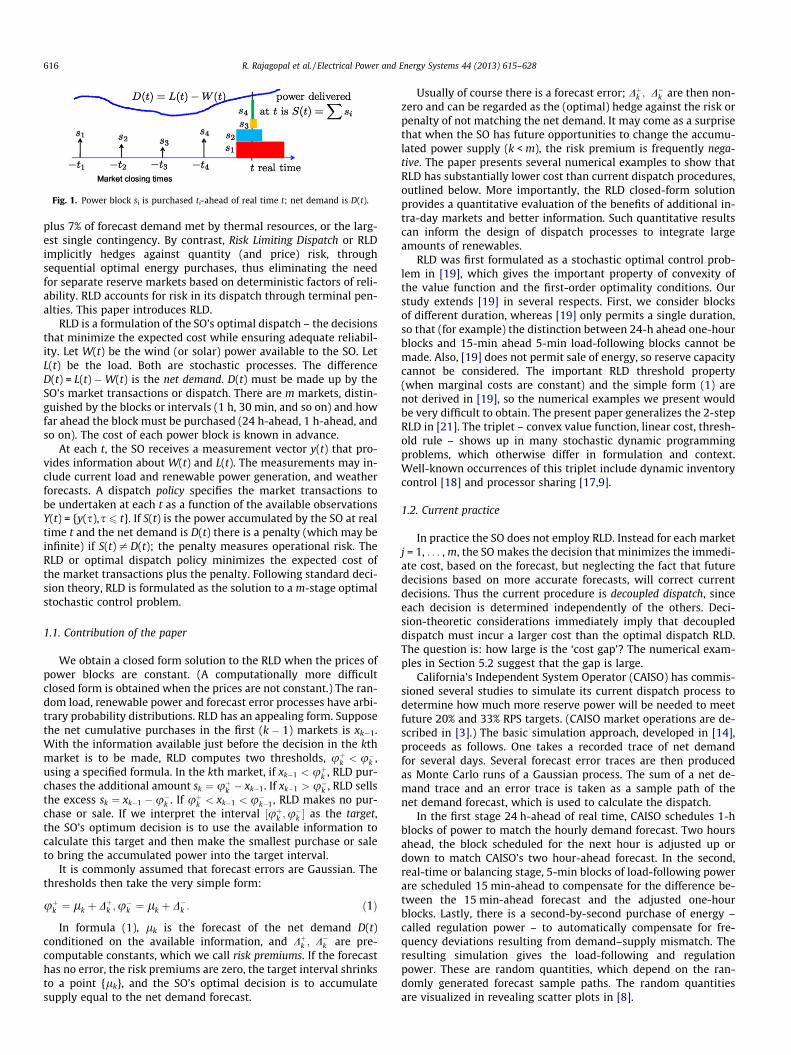
the real-time load. For example, in a four-step market process,the transactions might be staggered as follows (see Fig. 1):
� 24 h-ahead, SO purchases s1 for a 1 h block;� 1 h-ahead, SO purchases s2 for a 30 min block;� 15 min-ahead, SO purchases s3 for a 5 min block;� 5 min-ahead, SO purchases s4 for a 1 min block.
In addition to these forward or future energy purchases, the SOhedges against forecast errors and equipment failure by purchasingreserve capacity. A reserve capacity contract is a call option: uponpaying the option price, the SO secures the right but not the obli-gation to purchase energy in a particular forward market. We mod-el such a reserve capacity contract as a two-part transactioncomprising the purchase of a power block in a forward market fol-lowed by a sale of that power if the reserve capacity is not utilized.(The difference between the purchase and sale price is the price ofthe call option or the reserve capacity.) With this model there is noneed to distinguish between forward energy and capacity con-tracts, and the SO’s decisions comprises a sequence of forward en-ergy buy or sell transactions. The sequence of transactions is calledthe dispatch.
In practice the SO’s dispatch is much more elaborate: there aremarkets for up- and down load-following, regulation, and differenttypes of reserves, etc. In many of these transactions the SO followsrules-of-thumb. For example in CAISO (California Independent Sys-tem Operator) practice, the operating reserve requirement is set asthe maximum of 5% of forecast demand met by hydro resources
Fig. 1. Power block si is purchased ti-ahead of real time t; net demand is D(t).
616 R. Rajagopal et al. / Electrical Power and Energy Systems 44 (2013) 615–628
plus 7% of forecast demand met by thermal resources, or the larg-est single contingency. By contrast, Risk Limiting Dispatch or RLDimplicitly hedges against quantity (and price) risk, throughsequential optimal energy purchases, thus eliminating the needfor separate reserve markets based on deterministic factors of reli-ability. RLD accounts for risk in its dispatch through terminal pen-alties. This paper introduces RLD.
RLD is a formulation of the SO’s optimal dispatch – the decisionsthat minimize the expected cost while ensuring adequate reliabil-ity. Let W(t) be the wind (or solar) power available to the SO. LetL(t) be the load. Both are stochastic processes. The differenceD(t) = L(t) �W(t) is the net demand. D(t) must be made up by theSO’s market transactions or dispatch. There are m markets, distin-guished by the blocks or intervals (1 h, 30 min, and so on) and howfar ahead the block must be purchased (24 h-ahead, 1 h-ahead, andso on). The cost of each power block is known in advance.
At each t, the SO receives a measurement vector y(t) that pro-vides information about W(t) and L(t). The measurements may in-clude current load and renewable power generation, and weatherforecasts. A dispatch policy specifies the market transactions tobe undertaken at each t as a function of the available observationsY(t) = {y(s),s 6 t}. If S(t) is the power accumulated by the SO at realtime t and the net demand is D(t) there is a penalty (which may beinfinite) if S(t) – D(t); the penalty measures operational risk. TheRLD or optimal dispatch policy minimizes the expected cost ofthe market transactions plus the penalty. Following standard deci-sion theory, RLD is formulated as the solution to a m-stage optimalstochastic control problem.
1.1. Contribution of the paper
We obtain a closed form solution to the RLD when the prices ofpower blocks are constant. (A computationally more difficultclosed form is obtained when the prices are not constant.) The ran-dom load, renewable power and forecast error processes have arbi-trary probability distributions. RLD has an appealing form. Supposethe net cumulative purchases in the first (k � 1) markets is xk�1.With the information available just before the decision in the kthmarket is to be made, RLD computes two thresholds, uþk < u�k ,using a specified formula. In the kth market, if xk�1 < uþk , RLD pur-chases the additional amount sk ¼ uþk � xk�1. If xk�1 > u�k , RLD sellsthe excess sk ¼ xk�1 �u�k . If uþk < xk�1 < u�k�1, RLD makes no pur-chase or sale. If we interpret the interval ½uþk ;u�k � as the target,the SO’s optimum decision is to use the available information tocalculate this target and then make the smallest purchase or saleto bring the accumulated power into the target interval.
It is commonly assumed that forecast errors are Gaussian. Thethresholds then take the very simple form:
uþk ¼ lk þ Dþk ;u�k ¼ lk þ D�k : ð1Þ
In formula (1), lk is the forecast of the net demand D(t)conditioned on the available information, and Dþk ; D�k are pre-computable constants, which we call risk premiums. If the forecasthas no error, the risk premiums are zero, the target interval shrinksto a point {lk}, and the SO’s optimal decision is to accumulatesupply equal to the net demand forecast.
Usually of course there is a forecast error; Dþk ; D�k are then non-zero and can be regarded as the (optimal) hedge against the risk orpenalty of not matching the net demand. It may come as a surprisethat when the SO has future opportunities to change the accumu-lated power supply (k < m), the risk premium is frequently nega-tive. The paper presents several numerical examples to show thatRLD has substantially lower cost than current dispatch procedures,outlined below. More importantly, the RLD closed-form solutionprovides a quantitative evaluation of the benefits of additional in-tra-day markets and better information. Such quantitative resultscan inform the design of dispatch processes to integrate largeamounts of renewables.
RLD was first formulated as a stochastic optimal control prob-lem in [19], which gives the important property of convexity ofthe value function and the first-order optimality conditions. Ourstudy extends [19] in several respects. First, we consider blocksof different duration, whereas [19] only permits a single duration,so that (for example) the distinction between 24-h ahead one-hourblocks and 15-min ahead 5-min load-following blocks cannot bemade. Also, [19] does not permit sale of energy, so reserve capacitycannot be considered. The important RLD threshold property(when marginal costs are constant) and the simple form (1) arenot derived in [19], so the numerical examples we present wouldbe very difficult to obtain. The present paper generalizes the 2-stepRLD in [21]. The triplet – convex value function, linear cost, thresh-old rule – shows up in many stochastic dynamic programmingproblems, which otherwise differ in formulation and context.Well-known occurrences of this triplet include dynamic inventorycontrol [18] and processor sharing [17,9].
1.2. Current practice
In practice the SO does not employ RLD. Instead for each marketj = 1, . . . , m, the SO makes the decision that minimizes the immedi-ate cost, based on the forecast, but neglecting the fact that futuredecisions based on more accurate forecasts, will correct currentdecisions. Thus the current procedure is decoupled dispatch, sinceeach decision is determined independently of the others. Deci-sion-theoretic considerations immediately imply that decoupleddispatch must incur a larger cost than the optimal dispatch RLD.The question is: how large is the ‘cost gap’? The numerical exam-ples in Section 5.2 suggest that the gap is large.
California’s Independent System Operator (CAISO) has commis-sioned several studies to simulate its current dispatch process todetermine how much more reserve power will be needed to meetfuture 20% and 33% RPS targets. (CAISO market operations are de-scribed in [3].) The basic simulation approach, developed in [14],proceeds as follows. One takes a recorded trace of net demandfor several days. Several forecast error traces are then producedas Monte Carlo runs of a Gaussian process. The sum of a net de-mand trace and an error trace is taken as a sample path of thenet demand forecast, which is used to calculate the dispatch.
In the first stage 24 h-ahead of real time, CAISO schedules 1-hblocks of power to match the hourly demand forecast. Two hoursahead, the block scheduled for the next hour is adjusted up ordown to match CAISO’s two hour-ahead forecast. In the second,real-time or balancing stage, 5-min blocks of load-following powerare scheduled 15 min-ahead to compensate for the difference be-tween the 15 min-ahead forecast and the adjusted one-hourblocks. Lastly, there is a second-by-second purchase of energy –called regulation power – to automatically compensate for fre-quency deviations resulting from demand–supply mismatch. Theresulting simulation gives the load-following and regulationpower. These are random quantities, which depend on the ran-domly generated forecast sample paths. The random quantitiesare visualized in revealing scatter plots in [8].
R. Rajagopal et al. / Electrical Power and Energy Systems 44 (2013) 615–628 617
In order to simulate the impact of 20% or 33% RPS, the same ap-proach is followed in [2,4]. The only modification is that one mag-nifies recorded traces of renewable power to create traces thatmeet the RPS requirement. These studies find that large reservesare needed to absorb the variability of renewable power. For exam-ple, [12] concludes that ‘‘the amount of regulation and imbalance[load-following] energy dispatched in real time [. . .] to maintainsystem performance within acceptable limits during morning andevening ramp hours for 33% renewable cases in 2020 was4800 MW’’. Such fast-acting energy is costly, and may make meet-ing California’s 2020 goal of 33% renewable energy financiallyunsupportable. (The study admits that the 4800 MW requirementmay be ‘‘optimistic, in that the impact of large forecast errors forrenewable production, especially forecast errors associated withwind production, were not studied’’. Moreover, compensating var-iability in renewables with fast-acting thermal generation will re-duce the net GHG benefit of renewable energy.)
These simulation studies reveal that most of the reserve require-ments stem from CAISO’s practice of stacking only two kinds (1-hand 15-min) of power blocks. From Fig. 1 one can see that if renew-able power (part of D(t) in the figure) exhibits large intra-hour vari-ations (ramps), the burden of compensating for such variations willfall on the 5-min load-following blocks and the balancing energyneeds will be high. However, if CAISO were also to schedule shorterblocks (30-min, 15-min, etc.) at shorter times ahead – and hencewith lower forecast errors – the reserve requirements would belower. The increased flexibility gained by such intra-day marketsis advocated by NERC’s (North American Electric Reliability Coun-cil) Task Force on Integrating Variable Generation [11].
0
0
t
t
s(k1, k2)
s(k1, k2, ..., km)
T2
Tm
. . .
1.3. Limitations of the paper
The RLD presented here and the above-referenced simulationstudies have three limitations. First, they ignore transmission con-straints and losses. Second, they do not consider unit commitment(UC). UC introduces integer-valued decision variables that increasethe computational burden and preclude mathematical analysis.Studies such as [1,16] include UC start-up costs, but computationalcomplexity restricts them to a 2-stage dispatch, evaluated vianumerical examples. Consequently, these studies cannot predictthe reduction in needed reserves from intra-day markets or betterinformation. Note, moreover, that once the unit commitment deci-sion is made, RLD indeed determines the optimal power block pur-chases. Third, the paper does not consider storage devices ordemand-shaping programs that can absorb the variability ofrenewable power. The study [5] proposes the improvement ofwind generator controllability through the addition of a water stor-age plant.
The ‘‘current practice’’ description above is most suited to CAI-SO; other ISOs have somewhat different market structures and dis-patch procedures. The model of ‘wind power’ described more fullyin Section 2 is applicable to other unreliable sources such as solar;but it is not suitable for geothermal or hydro power, which aremuch more predictable.
The rest of the paper is organized as follows: The dispatch pro-cedure is formulated as an m-stage stochastic control problem inSection 2. The RLD optimality conditions are derived in Section 3.The special case of Gaussian forecast errors is treated in Section4. Two examples occupy Section 5. Conclusions are summarizedin Section 6. Proofs are collected in the Appendix.
ts(k1)
0
T1
Fig. 2. Supply S(t) is constructed by stacking blocks of duration T1, . . . , Tm.
2. Model of dispatch
The dispatch model specifies the SO’s energy supply, and for-mulates a dispatch policy and its cost.
2.1. Energy supply
Net load or demand is denoted by D(t) = L(t) �W(t), t P 0, withL(t) and W(t) being the true load and wind power. L and W are sto-chastic processes with arbitrary probability distributions. Time t isdiscrete, measured in hours. The dispatch constructs a supply S(t),t P 0, by stacking up blocks of power purchased in m markets.Blocks in the kth market have duration Tk, with T1 P � � �P Tm.We assume that Tj�1 is a multiple of Tj, Tj�1 = NjTj. These are theSO’s market transactions:
� SO buys (or sells) N1 blocks of magnitude s(k1) for the interval[k1T1, (k1 + 1)T1], k1 = 0, . . . , N1 � 1;� For each k1, SO buys (or sells) N2 blocks of magnitude s(k1,k2) for
the interval [k1T1 + k2T-2,k1T1 + (k2 + 1)T2], k2 = 0, . . . , N2 � 1;� For each k1, � � � , km�1, SO buys (or sells) Nm blocks of magnitude
s(k1, . . . , km) for the interval [k1T1 + � � � + kmTm,k1T1 + � � � +(km + 1)Tm].
By convention, s(k1, . . . , kj) > 0 or <0 accordingly as a power blockis purchased or sold. The power blocks of Fig. 2 are stacked to formthe energy supply function over the time horizon [0,N1T1], which ishours or days long.
The array of power blocks {s(k1, . . . , kj)} delivers power S(t) atreal time t:
Assumption (3) says that power must be purchased before it isdelivered. Typically the market closes a fixed time ahead, e.g.,t(k1) = k1T1 � 24 for the 24 h-ahead energy market. Assumption(4) is an intuitive requirement: block s(k1) must be purchased be-fore its sub-blocks s(k1,k2), which must be purchased before itssub-blocks s(k1,k2,k3), and so on.
We assume that the blocks s(k1), . . . , s(k1, . . . , km) can be se-lected independently. This assumption is violated if generators im-pose inter-temporal constraints on successive power blocks. Forexample, some generators have a minimum power-on duration,some have ramping constraints, and some (e.g. stored hydro) havea total energy constraint. (RLD extensions that permit such con-straints would be significant contributions.)
618 R. Rajagopal et al. / Electrical Power and Energy Systems 44 (2013) 615–628
The net demand D(t) = L(t) �W(t) is random because the loadL(t), wind power W(t), or both are random. Forced outages of gen-eration or other equipment are readily modeled as random in-creases in load as in [6]. At time t an observation y(t) providesinformation about the net demand. The observations up to t com-prise the array Y(t) = {y(s),s 6 t}.
The selection of block s(k1, . . . , kj) is based on the availableinformation, so s(k1, . . . , kj) is a function of Y(t(k1, . . . , kj)). Formallys(k1, . . . , kj) is adapted to the r-field Yðtðk1; . . . ; kjÞÞ generated bythe random variables Y(t(k1, . . . , kj)). A dispatch policy p for theinterval [0,N1T1] is any array of functions,
p ¼ fsðk1; . . . ; kjÞ is adapted to Yðtðk1; . . . ; kjÞÞg: ð5Þ
An initial block of power z(k1) has been secured ahead of timek1T1, as the result of actions (such as must-run generation) takenbefore our decision problem. If z(k1) is random, it must beY(t(k1))-adapted, so its value is known when s(k1) is to be selected.
Let x(k1, . . . , kj) be the total power secured just after s(k1, . . . , kj)is selected:
We regard x(k1, . . . , kj) as the state and s(k1, . . . , kj) as the deci-sion at stage (k1, . . . , kj), based on the observations Y(t(k1, . . . , kj)).The state satisfies the update equation (see Fig. 3):
s(k1, . . . , kj) may be positive or negative accordingly as power is pur-chased or sold. The power eventually delivered at real time t 2 [k1-
2 [k1T1 + � � � kmTm,k1T1 + � � � (km + 1)Tm] is x(k1, . . . , km). The(random) net demand during interval is denoted d(k1, . . . , km).
2.3. Cost and penalty
The cost of block s = s(k1, . . . , kj) is a known convex functionC(k1, . . . , kj;s). At first, we consider the case when the marginal costis constant:
c+(k1, . . . , kj) and c�(k1, . . . , kj) are unit prices for buying and sellingpower during [k1T1 + � � � kjTj, k1T1 + � � � (kj + 1)Tj] so the cost of blocks(k1, . . . , kj) is
In (8), E denotes mathematical expectation. Except for the lastterm, the right hand side in (8) is the energy cost for the interval[0,N1T1]. In the last term in (8) d(k1, . . . , km) is the net demand,x(k1, . . . , km) is the power supplied, and Tm[g(d(k1, . . . , km),x(k1, . . . , km))] is the risk or penalty of imbalance during[k1T1 + � � � + kmTm, k1T1 + � � � + (km + 1)Tm]. The total cost J(p) is en-ergy cost plus the imbalance penalty.
Risk-limiting dispatch or RLD is the policy p⁄ that minimizes thecost J(p):
Jðp�Þ ¼minp
JðpÞ
s:t: ð5Þ ð9Þ
RLD p⁄ is determined in Section 3 under the following restrictionson the prices c+, c� and the penalty g.
Restriction on prices In order to avoid trivial cases the pricessatisfy
Suppose to the contrary that c+(k1, . . . , kj+1) < c+(k1, . . . , kj). Thenthe cost (8) is reduced by postponing purchase of s+(k1, . . . , kj) fromtime t(k1, . . . , kj) to the later time t(k1, . . . , kj+1) (see (4)), so s+
(k1, . . . , kj) will be zero. Similarly, if c�(k1, . . . , kj+1) > c�(k1, . . . , kj),the cost is lowered by postponing the sale of s�(k1, . . . , kj) to the la-ter time t(k1, . . . , kj+1), so s�(k1, . . . , kj) will be zero. Lastly, if c+(k1, -+(k1, . . . , kj) < c�(k1, . . . , kj) the SO can make arbitrarily large profitssimply by buying and selling equal amounts s+(k1, . . . , kj) = s�(k1,. . . , kj), which is not meaningful. One consequence of (10) is thatin any cost-minimizing policy, one will have
gðd; xÞ is nonnegative and convex in x for each d: ð12Þ
, kj) as a function of Y(t(k1, . . . , kj)).
R. Rajagopal et al. / Electrical Power and Energy Systems 44 (2013) 615–628 619
We present important forms of penalty below. In many casesg(d,x) is decreasing in x.
Value of lost load (VOLL) With
gðd; xÞ ¼ cþðk1; . . . ; kmÞ½d� x�þ; ð13Þ
Tm[g(d(k1, . . . , km), x(k1, . . . , km))] is the value of lost load (VOLL) in[k1T1 + � � � + kmTm,k1T1 + � � � + (km + 1)Tm] when the supply is insuffi-cient to serve the demand. c+(k1, . . . , km) is the social cost of powerinterruption, conventionally assessed at $1000–10,000 per MW h. gspecified by (13) is decreasing and convex.
Loss of load probability (LOLP) Because it accounts for uncer-tainty, LOLP is considered a better measure of reliability than thetraditional deterministic ‘reserve margin’, especially when inter-mittent sources are significant [6]. The use of LOLP to specify a risktarget in system operations is also advocated in [15,23]: the dis-patch must be such that the LOLP during the interval [0,N1T1] isbounded by a pre-specified target value a P 0. This is equivalentto the constraint
g specified by (15) is decreasing and convex in x. Resorting to infi-nite values in (15) can be eliminated by the following observation.The least supply x with LOLP at most a is the a-quantile Ua:
the reserve; then RaRa = x(k1, . . . , km) �Ua(k1, . . . , km) is the re-serve-at-risk (at level a). At time t(k1, . . . , km) the net demand d(k1, -. . . , km) and hence the reserve r may not be known. But because of(16), the reserve-at-risk RaRa is known. As
the reserve r falls below RaRa with probability at most a. Equiva-lently (17) ensures that the reserve exceeds RaRa with probabilityat least (1 � a).
If there is agreement about the appropriate value of a (say, 1%),RaRa can serve as a reserve target for the SO. At any time a negativeRaRa indicates that SO should increase the reserve by the sameamount in order to maintain the required level of operational reli-ability, but with a positive RaRa the operator knows that the reli-ability level is higher than required [23].
Conditional reserve at risk The event that the reserve dropsbelow RaRa occurs with probability a, and one measure of the riskwhen this event occurs is the conditional reserve at risk:
CRaRa¼�Efrjr<RaRa;Yðtðk1; . . . ;kmÞÞg¼1a
Z 1
Ua
ðd�xÞpðdÞdd; ð19Þ
in which r = x � d = x(k1, . . . , km) � d(k1, . . . , km), p(d) = p(d = djY(t(k1, . . . , km))) is the probability density of the net demand d con-ditional on Y(t(k1, . . . , km)). The interpretation of (19) is this. Sup-pose at some time t(k1, . . . , km), RaRa = 100 MW, CRaRa = 600 MW.Then the loss of load is expected to be 600 MW if the reserve dropsbelow 100 MW. CRaRa is decreasing and convex in x. There areinstructive calculations of RaRa and CRaRa in [23].
Cost of excessive generation Random large amounts of windpower can cause net demand d = d(k1, . . . , km) to drop below thesupply x = x(k1, . . . , km). A penalty may then be assessed
gðd; xÞ ¼ c�ðk1; . . . ; kmÞ½x� d�þ;
which may be combined with (13) into the convex penalty function
gðd; xÞ ¼ cþ½d� x�þ þ c�½x� d�þ:
In this case, it may be less costly to curtail wind at stage m, soRLD would select s⁄(k1, . . . , km) < 0. Alternatively, one may replace(14) with
and define the risk from wind on-ramps as a ‘wind curtailment atrisk’ (WCaR) similarly to RaR.
2.4. Wind aggregator
A wind aggregator may contract to deliver blocks of firm powerL(k1) at a fixed price c�(k1) during [k1T1, (k1 + 1)T1]. The contractedpower combines wind W(t) and conventional power supply S(t).The aggregator wants to minimize the expected net cost,
�X
k1
c�ðk1ÞLðk1Þ þ JðpÞ;
in which the first term is the negative of the revenue and the secondterm is the cost (8). The aggregator’s RLD gives the optimum blocksL⁄(k1) that the aggregator should contract. The aggregator’s cost iswell modeled by constant prices, whereas the SO’s cost may be bet-ter specified by a cost function.
3. Optimality conditions
Most of this section is concerned with the case of constantprices. The case of a cost function is treated in Theorem 3. Forany policy p the cost-to-go in state x = x(k1, . . . , kj�1) at stage(k1, . . . , kj) conditional on the information available at t(k1, . . . , kj)is (see Fig. 3)
620 R. Rajagopal et al. / Electrical Power and Energy Systems 44 (2013) 615–628
denote the conditional expectation and conditional probability of therandom variable v and event A.
Proof. See Appendix B. h
Theorem 3 deals with the case when the marginal cost is notconstant. The cost of policy p is
JðpÞ ¼ E T1
XN1�1
k1¼0
Cðk1; s1ðk1ÞÞ þ T2
XN1�1
k1¼0
XN2�1
k2¼0
Cðk1; k2; sðk1; k2ÞÞ þ � � �(
þTm
XN1�1
k1¼0
XN2�1
k2¼0
� � �XNm�1
km¼0
½Cðk1; . . . ; km; sðk1; . . . ; kmÞÞ
þgðdðk1; . . . ; kmÞ; xðk1; . . . ; kmÞÞ�g:
Above, C(k1, . . . , kj; s) is convex in s, and s > 0 or <0, accordinglyas a block is purchased or sold. g(d, �) is the convex terminal pen-alty. The value function is defined in (20).
Lemma 1 holds with obvious changes: in state x = x(k1, . . . , km�1),
and for j 6m � 1, in state x(k1, . . . , kj�1) at stage (k1, . . . ,kj),
J�ðx;k1; .. .;kjÞ¼ infs
TjCðk1; .. . ;kj; sÞþXNjþ1�1
kjþ1¼0
E½J�ðxþs;k1; .. . ;kjÞjYðtðk1; .. . ;kjÞÞ�
8<:9=;a:s:
ð38Þ
Moreover, the minimizing s in (37) and (38) is the optimumdecision.
Theorem 3. The value function J⁄(x,k1, . . . , kj), j 6m, is convex andYðk1; . . . ; kjÞ-adapted. The optimum decision s⁄(k1, . . . , km) in statex = x(k1, . . . , km�1) at the terminal stage (k1, . . . , km) is the solution s of
Thus the new observation at t(k1, . . . , kj) adds the ‘correction’�(k1, . . . , kj�1) to the previous forecast l(k1, . . . , kj�1) and reducesthe error variance by r2(k1, . . . , kj�1).
The optimal decision in state x = x(k1, . . . , kj�1) is given by:
s�ðx;k1; . . .;kjÞ¼/þðk1 ;. . . ;kjÞ�x; if /þðk1; . .. ;kjÞ�x>00; if /þðk1; . .. ;kjÞ< x</�ðk1; . .. ;kjÞ�½xðk1 ;. . . ;kj�1Þ�/�ðk1; . . . ;kjÞ�; if /�ðk1; . .. ;kjÞ< x
8><>:ð49Þ
If the supply x acquired up to stage (k1, . . . , kj) is smaller than thelower threshold, an energy block equal to the shortfall must be pur-chased; if the acquired supply is larger than the upper threshold,the excess must be sold.
5. Two examples
Two examples are worked out in this section. The first uses for-mulas (32)–(34). The second uses formula (46) for the Gaussiancase. To simplify the notation and calculations we assume
We write c+(k) = c(k). Because c�(j) = 0, it does not pay to sellany capacity, so s��ðjÞ ¼ 0, and we write s (j) = s+(j), s�(j) = 0. Thedecision s(j) is taken at time t(j). The thresholds are denotedu+(j) = u(j) and u�(j) =1 (which is equivalent to s��ðjÞ ¼ 0).
The cost of policy p is
JðpÞ ¼ EXm
j¼1
cðjÞsðjÞ þ gðdðmÞ; xðmÞÞ( )
:
The RLD dispatch is
s�ðjÞ ¼ ½uðjÞ � xðj� 1Þ�þ:
We assume that d(m) is observed at the last decision time t(m),and require the net demand to be met with probability one. So thepenalty is (15) with a = 0. Write c(m + 1) =1. Then rg(d,x) = �c(m + 1)1(x < d), so (31) and (32) give the threshold in stage m,
uðmÞ ¼ dðmÞ: ð50Þ
Henceforth we write d(m) = d. For j 6m � 1, (31)–(34) showthat the threshold u(j) is the solution x of the equation
In (53), Pj(v) is the probability of event v, conditioned on Y(t(j)).Expression (53) is evaluated in reverse order j = m � 1, . . . , 1, start-ing with u(m) = d. At stage (m � 1)
Fm�1ðxÞ ¼ 1� Pm�1ðx 6 uðmÞÞ ¼ Pfx < djYðtðm� 1ÞÞg
¼ cðm� 1ÞcðmÞ : ð54Þ
Fig. 4 depicts Fm�1(x), and shows that u(m � 1) is the c(m � 1)/c(m)-quantile of Fm�1(x) = P{d P xjY(t(m � 1))}. u(m � 1) is a func-tion of Y(t(m � 1)).
We now evaluate Fm�2(x) from (53):
Fm�2 ¼ Pm�2ðx 6 uðm� 1ÞÞ þ cðmÞcðm� 1Þ Pm�2ðx
6 uðmÞ;uðm� 1Þ < xÞ ¼ Pfx
6 uðm� 1ÞjYðtðm� 2ÞÞg þ cðmÞcðm� 1Þ Pfuðm� 1Þ < x
< djYðtðm� 2ÞÞg ¼ cðm� 2Þcðm� 1Þ : ð55Þ
Thus u(m � 2) is the c(m � 2)/c(m � 1)-quantile of the comple-mentary distribution function Fm�2(x). From (55) we see that tocalculate Fm�2(x) one needs the joint distribution of u(m � 1) andu(m) = d, conditioned on Y(t(m � 2)). In general, the calculationof u(j),Fj(x) needs the joint distribution of u(m) = d,u(m � 1), . . . , u(j + 1), conditioned on Y(t(j)). The calculation canbe automated to fit the form of the observations.
5.1. Example 1
Take m = 3, c(1) = 50, c(2) = 100, c(3) = 1,000. Purchases aremade at t(1), t(2), t(3). At t(3), d is observed, so
uð3jdÞ ¼ d:
At t(2) a forecast arrives. It has two possible values, L (low de-mand) or H (high demand), each with probability 0.5. The distribu-tion of d conditioned on the forecast is
PðdjLÞ ¼ U½�2; 1�; PðdjHÞ ¼ U½�1; 2�:
(U[a,b] is the uniform distribution over [a,b]). The threshold atstage 2 is given by solving (55):
Using P(djL) = U[�2,1], P(djH) = U[�1,2] in (55) gives an explicitexpression for F2(xjx). The result if plotted in the right panel ofFig. 5. Solving for the 0.1-quantiles in (56) gives the stage 2threshold:
uð2jLÞ ¼ 0:7; uð2jHÞ ¼ 1:7:
We proceed to stage 1 assuming no information is available(Y(t(1)) = ;), so (54) is
Fig. 4. Threshold u(m � 1) is the c(m � 1)/c(m)-quantile of Fm�1.
Fig. 5. Information structure (left) and thresholds (right) for Example 1.
R. Rajagopal et al. / Electrical Power and Energy Systems 44 (2013) 615–628 623
Substituting for the probabilities and the threshold u(2) gives theexpression for F1(x), which is plotted in the right panel. By (54),the optimal threshold u(1) is the c(1)/c(2) = 0.5-quantile of F1(x),which can be read off from Fig. 5: u(1) = 1.
The minimum expected cost is smaller when the stage 2 fore-cast is available. Surprisingly, the cost savings occur when net de-mand is low. For instance if d < 1 (which occurs with probability 5/6), the after-forecast decision s⁄(1) = 1 is better than the wastefulno-forecast decision s⁄(1) = 1.67. But for d > 1.67, (which occurswith probability 1/18), the no-forecast decision is better, since itpurchases 1.67 units at a lower cost. Observe that the currentlypracticed decoupled dispatch ignores the existence of the laterdecision, so its decision in stage 1 would be 1.67. For an empiricalstudy of wind forecast in Germany and Greece see [10].
5.2. Example 2
We now consider several examples in which the forecast errorsare Gaussian, although the net demand d(m) = d need not be Gauss-ian. Theorem 4 applies, and the thresholds are given by (46):
uðjÞ ¼ lðjÞ þ DðjÞ: ð58Þ
The forecast l(j), based on Y(t(j)), has the error
d� lðjÞ ¼ �ðjÞ þ � � � þ �ðmÞ; ð59Þ
�(j), . . . , �(m) are independent zero-mean Gaussian random vari-ables with variances r2(j), . . . , r2(m).
At stage m, d is observed, so l(m) = d, r2(m) = 0,u(m) = d. Atstage (m � 1) by (54),
Since conditional on Y(t(m � 2)),�(m � 1),�(m � 2) are indepen-dent Gaussian random variables with zero mean and variancesr2(m � 1),r2(m � 2), we can evaluate these two probabilities, andthen express Fm�2(x) as a function Wm�2(x � l(m � 2)) that doesnot depend on Y(t(m � 2)). D(m � 2) is then obtained by solving
Wm�2ðDðm� 2ÞÞ ¼ cðm� 2Þcðm� 1Þ : ð65Þ
The optimum threshold is then given by
uðm� 2Þ ¼ lðm� 2Þ þ Dðm� 2Þ:
As expected, the risk premium D(m � 2) can be pre-computedfrom (65). We can proceed in this way through stagesm � 3, . . . , 1. We consider some numerical examples.
Example 2A. 2-stage vs 10-stage dispatch We first specify thedifferent components of the model. As before, the net demandd(m) = d must be met with probability 1. d can take positive ornegative values. We divide d by its maximum value dmax, so�1 6 d 6 1, but nevertheless refer to d/dmax as d.
For the remainder of this section t(j) denotes the time horizon(previously t � t(j)) for stage j, so t(j) ? 0 as j ? m.
Forecast error The percentage error as a function of forecasthorizon from 0 to 24 h (day-ahead) is given by the plot of Fig. 6.The errors are Gaussian, and the percentage error is the ratio of the
Fig. 7. Minimum expected normalized cost conditioned on d, for three strategies.The unnormalized cost is obtained by multiplying by $72.
624 R. Rajagopal et al. / Electrical Power and Energy Systems 44 (2013) 615–628
standard deviation to dmax. Since d is normalized, the percentageerror is also the standard deviation of the forecast error. For anyhorizon t, l(t) is the forecast, �(t) is its error, and r(t) is its standarddeviation. That is,
lðtÞ ¼ d� �ðtÞ;E�ðtÞ ¼ 0;E�2ðtÞ ¼ r2ðtÞ:
For example, from the plot, r(24) = 0.17, r(9.1667) = 0.161, andso on. These forecast errors are considered the best currently pos-sible. By contrast, CAISO regards any forecast with a horizon of 6 has unreliable, whereas according to the figure the error at 6 h isonly r(6) = 0.09.
Stages We consider a maximum of 10 stages. The time of thestages are chosen so that each stage reduces the uncertainty by10%. That is, the time horizons are obtained by dividing themaximum uncertainty in the plot (which is 17% 24-h ahead) by 10and taking the corresponding ‘forecast horizon’ intercepts. Thisprocedure leads to the following sequence of horizons:
Thus, the maximum percentage error 24-h ahead is 17%, per-centage error in stage 1 (9.1667- h ahead) has decreased to(0.9 � 17)%, and so on. At stage 10 (0.0003-h ahead), the error is0%, i.e. the net demand is completely known. The stages are shownby the circles in the plot.
Several optimal RLD strategies are considered. They differ in thesubset of the 10 stages for which intra-day markets are available.As a benchmark we also consider the oracle case in which demandis known 24 h ahead.
Prices The forward prices for the intra-day markets are deter-mined as follows. From CAISO data, we take the 24-h aheadpurchase price to be $52 per MW h, the load-following price (5-min ahead) to be $60 per MW h and the real-time price (at stage10) to be $72 per MW h, corresponding to a load-following andregulation-up reserve capacity price of $8 and $20 per MW,respectively. The price at any stage with time horizon t h isobtained by an exponential fit: p(t) = A + Be�ct. That is, A, B, c areselected so that p(24) = 52, p(5 min) = 60, p(0) = 72. CAISO pricesare averages over the year: on any given day they deviateconsiderably from these averages. This is useful to note since theoptimal dispatch depends significantly on these prices. Supposes(j) is purchased in stage j. We require
P101 sðjÞ � d P 0 wp 1. In
Example 2B the zero LOLP constraint is replaced by a VOLL penalty.RLD strategies The optimal dispatch is calculated and compared
1. 2-stages: stages 1 (24-ahead) and 10 (real-time).2. 10-stages: all stages in the plot.3. Oracle: at stage 1, d is known, so oracle strategy purchases
s(1) = d+, at the lowest price.
The minimum cost for strategies 1, 2 and 3 is successivelylower. The RLD decision at stage j is
s�ðjÞ ¼ ½uðjÞ � xðj� 1Þ�þ ¼ lðjÞ þ DðjÞ: ð66Þ
The risk premium D(j) is pre-calculated.Results We make no assumptions about the distribution of d.
Instead we calculate the optimal cost conditional on the realizationof d as follows:
1. Select any realization of d 2 [�1,1].2. Generate 100 independent samples of the errors �(j) according
to Nð0;r2ðjÞÞ.3. For each d and error sample calculate the corresponding realiza-
tions of the forecast l(j) from (59), the optimal decision from(66), and the cost of the sample realization,
1 Forthis art
cð1Þs�ð1Þ þ � � � þ cðmÞs�ðmÞ:
The average of these 100 random costs is an estimate of the mini-mum expected cost for each RLD strategy, conditioned on d. Fig. 7displays their costs.In Fig. 7 the cost is normalized by $72. Since 52/72 = 0.72, and theoracle strategy purchases d+, its cost is 0.72 � d+, which is the bot-tom or red1 plot. The green and blue plots are the 2-stage and 10-stage costs, respectively. As expected, the blue curve is below thegreen curve. Both strategies make purchases even if (in hindsight)d turns out to be negative. (Unlike the red plot, the green and blueplots are not straight lines, despite their appearance.) The normal-ized 10-stage cost is lower than the 2-stage cost by about 0.05 or(0.05 � 72) = 3.6 $/MW h. This is a large savings in view of esti-mates of operating energy reserve costs of 2.5–5.0 $/MW h [20].
Fig. 8 is a plot of the relative savings, defined as the ratio (2-stage cost-10-stage cost)/(2-stage cost), conditioned on d. Thesavings approach 70% for small values of d, and decrease for d
interpretation of color in Fig. 7, the reader is referred to the web version oficle.
Fig. 8. Relative savings of 10-stage vs. 2-stage strategy, conditioned on d. Fig. 9. Additional cost of 2-stage and 10-stage strategies relative to oracle strategy.
R. Rajagopal et al. / Electrical Power and Energy Systems 44 (2013) 615–628 625
positive and large, as more and more purchases in the 10-stageproblem are made towards real time. Thus the 2-stage is relativelymore wasteful (excessive reserves are purchased) when d is small.At d = 0.4 the difference is about 0.5, that is, the 10-stage dispatchpurchases only one-half the energy of the 2-stage dispatch.
Fig. 9 plots the additional minimum expected cost of the 2-stage and 10-stage strategies relative to the oracle strategy. Againwe see that the relative impact of additional information and morestages is more pronounced for small values of d.
The impact of more stages and additional information can alsobe assessed from Fig. 10, which plots the risk premium D(i) vsstage number. (Stage 11 is for t = 0.) The premium is large andnegative in the early stages, approaching 0 at real time. Thenegative premium means (see (66)) that it is optimal to maintainreserves below the forecast demand since the forecast may turn outto be too high, with compensating purchases at later stages.
Fig. 10. Risk premium vs stage number.
Example 2B. 2-stage vs 4-stage and VOLL In Example 2A the laststage (stage 10) is at real time, when there is no forecast error andthe reserve cost is $72 per MW h. In practical terms, this should betaken as the cost of lost load, valued at $1000–10,000 per MW h.We compare three RLD dispatches. In the 2-stage problem, thestage 1 cost is $52/MW h, and VOLL is $1000/MW h. The 4-stageproblem has two additional stages: a 1-h ahead stage at a cost of$60/MW h and a 15-min ahead stage at a cost of $72/MW h. Inthe oracle case, the 24-ahead forecast has no error. Fig. 11 providesa comparison of the minimum expected cost, conditioned on d, forthe three optimal dispatches. The actual cost is obtained by multi-plying the normalized cost by $1000.
The effect of a VOLL penalty is gauged by comparing the plots ofFig. 11 with those in Fig. 7. Evidently, a large VOLL increases the valueof additional information and more stages. The additional normal-ized cost incurred by the 2-stage dispatch is at 0.015 or $15 perMW h. (This is much larger than the range 2.5.5.0 $/MW h, whichdoes not include VOLL.) Again, the 2-stage cost is higher when netdemand is low. For example, when d = 0, the minimum cost for the 2-stage dispatch is $15 (0.015 � 1000) vs $1 for the 4-stage dispatch.
Fig. 11. Minimum expected normalized cost conditioned on d, for three strategies.The $ cost is obtained by multiplying by $1000/MW h.
Example 2C. 2-stage vs 3-stage, different forecast errors In thelast example we consider a 2-stage (stages 1,2) vs a 3-stage (stages1,2,3) RLD dispatch with costs of $52, $60 and $72, and a VOLL of$1000. We consider three levels of forecast error: best casedenoted 1X (standard errors of Fig. 6), medium case denoted 2Xwith twice the standard error, and the worst case denoted 3X withthrice the standard error.
Fig. 12. Comparison of minimum average cost for 2-stage vs 3-stage dispatch, conditioned on d for best (1X), medium (2X), and worst (3X) forecast errors. The y-axis scalesare different.
626 R. Rajagopal et al. / Electrical Power and Energy Systems 44 (2013) 615–628
Fig. 12 gives the additional cost in the three cases incurred bythe 2-stage dispatch, conditioned on the net demand d. (Note: thevertical scales are different.) The benefits are large: the 2-stage costis larger than the 3-stage cost by about $2.5 per MW h for the 1Xcase, $4.5 per MW h for the 2X case and $9.0 per MW h for the 3Xcase. This shows that having more stages (closer to real time)compensates for better forecasts.
6. Conclusions
A system operator’s dispatch is a sequence of decisions to bal-ance the supply and load of electric power at every instant, inthe face of forecast errors about future load and renewable gener-ation. The decisions comprise purchases of blocks of energy and re-serve capacity (call options) in different markets, with each blockgetting shorter as real time approaches. The decisions are basedon the information available at the times when the relevant marketcloses. In current practice, the decisions are decoupled: the SOminimizes the expected cost of each decision, ignoring the fact thatsubsequent decisions can correct for current errors. The presentpaper formulates the dispatch as a stochastic control problem,which takes future decisions into account in determining the cur-rent decision.
The optimal or risk-limiting dispatch (RLD) is found in ‘closed-form’ as a solution of the corresponding stochastic dynamic pro-gram. In the case of constant prices, RLD has a very attractive form:at each stage, one calculates two thresholds based on the availableinformation. The SO’s task is to acquire or sell energy so that theaccumulated energy is between the two thresholds. In the casethat the forecast errors are Gaussian, the thresholds can be pre-computed. When the SO faces a convex cost function, the RLDcalculations are more complicated.
The closed-form formulas permit the comparison of optimaldispatch processes in terms of the number of stages, price and pen-alty structure and the available information. As expected, the costis lower as the number of stages increase or the forecast errors de-crease. The cost reductions can be large: the addition of one or twointra-day markets (with correspondingly better forecasts) can re-duce reserve energy costs by 50 percent in comparison with pub-lished estimates.
The comparison points towards two operational improvementsthat merit further investigation. First, it seems that California Inde-pendent System Operator (CAISO) could benefit greatly by addingintra-day and intra-hour decisions to its current day-ahead andreal-time balancing markets. Adding these decisions implies thatCAISO’s traditional separation of day-ahead, load-following, andregulation power (which is reflected in a corresponding separationof generation resources) may no longer be appropriate. Instead, theSO should simply group those resources by how quickly they cansupply power. The cost of such market changes is, however, also
large, as they will necessitate new procedures and software notonly for the market ‘maker’ CAISO but also the market partici-pants–generators and load-serving entities. Second, the benefit de-rived from improved forecast accuracy appears equally significant.The cost of improving forecasts through more sensors and betteralgorithms should be much less than implementing new markets.
In addition to system operators, the models and results in thepaper may be used to formulate the problem faced by a wind‘aggregator’ who must absorb the wind power variability with re-serve energy, and sell the resulting firm power.
The paper has several limitations. Unit commitment or genera-tor start-up costs are not included, because they add integer-valued decision variables. However, the results presented hereremain useful after the unit commitment decisions. Transmissionconstraints are ignored in the paper’s single-bus model. Pricesare assumed known ahead of time. Lastly, inter-temporal storageor ramping constraints are also not treated.
Acknowledgements
This research was supported by NSF Awards 1129001 and1135872, CERTS, and Inst for Adv Study, HKUST. The authors aregrateful to Janusz Bialek, Chris Dent, Robert Entriken and Kamesh-war Poolla for discussions that significantly improved the paper.
Appendix A. Proof of Theorem 1
The proof is based on Lemma 3.
Lemma 3. Let V (x), x P 0, be Y-adapted and convex. Let C (z), z 2 R,be convex. Let Y0 Y be a sub-r-field. Denote
R. Rajagopal et al. / Electrical Power and Energy Systems 44 (2013) 615–628 627
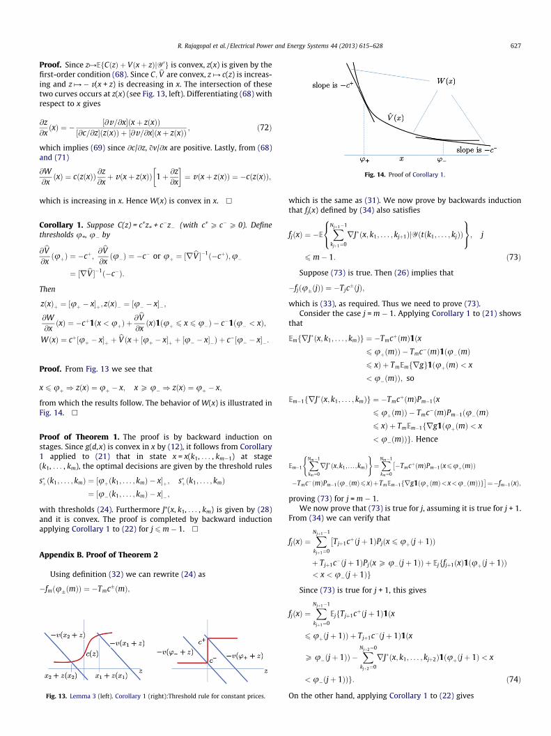
Proof. Since z#EfCðzÞ þ Vðxþ zÞjY0g is convex, z(x) is given by thefirst-order condition (68). Since C; bV are convex, z ´ c(z) is increas-ing and z ´ � v(x + z) is decreasing in x. The intersection of thesetwo curves occurs at z(x) (see Fig. 13, left). Differentiating (68) withrespect to x gives
@z@xðxÞ ¼ � ½@v=@x�ðxþ zðxÞÞ
½@c=@z�ðzðxÞÞ þ ½@v=@x�ðxþ zðxÞÞ ; ð72Þ
which implies (69) since @c/@z, ov/@x are positive. Lastly, from (68)and (71)
@W@xðxÞ ¼ cðzðxÞÞ @z
@xþ vðxþ zðxÞÞ 1þ @z
@x
� �¼ vðxþ zðxÞÞ ¼ �cðzðxÞÞ;
which is increasing in x. Hence W(x) is convex in x. h
Corollary 1. Suppose C(z) = c+z+ + c�z� (with c+ P c�P 0). Definethresholds u+, u� by
from which the results follow. The behavior of W(x) is illustrated inFig. 14. h
Proof of Theorem 1. The proof is by backward induction onstages. Since g(d,x) is convex in x by (12), it follows from Corollary1 applied to (21) that in state x = x(k1, . . . , km�1) at stage(k1, . . . , km), the optimal decisions are given by the threshold rules
with thresholds (24). Furthermore J⁄(x, k1, . . . , km) is given by (28)and it is convex. The proof is completed by backward inductionapplying Corollary 1 to (22) for j 6m � 1. h
which is the same as (73), as required. Lastly, fj is decreasing sinceJ⁄(x, k1, . . . , kj+1) is convex. h
Appendix C. Proof of Theorem 3
The proof imitates the proof of Theorem 1 with an application ofLemma 3. h
Appendix D. Proof of Lemma 2
To simplify notation, we write l(j) = l(k1, . . . , kj), �(j) = �(k1, . . . ,kj), and so on, and c+ = c+(k1, . . . , km). Since g(d,x) = c+[d � x]+,rg(d,x) = � c+1(d� x P 0), and so from (32),
fmðxÞ ¼ TmcþPmðdðmÞ � x P 0Þ ¼ TmcþPmð½lðmÞ � x� þ �ðmÞP 0Þ:
By (44), under Pm the random variable [l(m) � x] + �(m) isGaussian with mean [l(m) � x] and variance r2(m). Hence thefunction w(k1, . . . , km, �) defined by
wðk1; . . . ; km; x� lðmÞÞ ¼ TmcþPmðdðmÞ � x P 0Þ; ð76Þ
is deterministic, which establishes (45) and hence (46) for j = m.We proceed to j = m � 1. By (34),
Under distribution Pm�1, the random vector (�(m � 1) +[l(m � 1) � x], �(m � 1) + �(m) + [l(m � 1) � x]) is Gaussian withmean [l(m � 1) � x] e where e is a vector of all 1’s, and covariancematrix QRQT with R = diag{r2(m � 1),r2(m)} and
Q ¼1 01 1
� �:
It follows that Pm�1 of each of the three events is a function of[l(m � 1) � x]. This proves (45) for j = m � 1.
Suppose now that (45) and hence (46) hold for j + l,l P 1. Weshow that (45) holds for j. From (34) we see that fj(x) is a linearcombination of probabilities (under Pj) of intersections of eventsof the form
is Gaussian with mean [l(j) � x]e where e is a vector of all 1’s, andcovariance matrix QRQT with R = diag{r2(j), . . . , r2(m)} and
Q ¼
1 0 � � � 01 1 � � � 0
� � �1 1 � � � 1
2666437775:
So each probability in (34) can be expressed as explicit integralsof this multivariate distribution, hence as explicit functions of[l(j) � x]. This proves (45) for j. h
References
[1] Bouffard F, Galiana FD. Stochastic security for operations planning withsignificant wind power generation. IEEE Trans Power Syst 2008;23(2):306–16.
[2] California ISO. Integration of renewable resources: transmission and operatingissues and recommendations for integrating renewable resources on theCalifornia Iso-controlled grid. Technical report, California ISO; 2007.
[3] California ISO. CAISO business practice manual for market operations, Version13. Technical report, California ISO, October 2010.
[4] California ISO. Integration of renewable resources: operational requirementsand generation fleet capability at 20% RPS. Technical report, California ISO;2010.
[5] Castronuovo ED, Lopes JAP. Optimal operation and hydro storage sizing of awind-hydro power plant. Int J Electr Power Energy Syst 2004;26(10):771–8.
[6] Doherty R, O’Malley M. A new approach to quantify reserve demand in systemswith significant installed wind capacity. IEEE Trans Power Syst 2005;20(2):587–95.
[7] EnerNex Corporation. Eastern wind integration and transmission study.Subcontract Report NREL/SR-550-47078, National Renewable EnergyLaboratory; 2010. <http://www.nrel.gov/wind/systemsintegration/pdfs/2010/ewits_final_report.pdf>.
[8] Makarov YV, et al. Incorporating wind generation and load forecastuncertainties into power grid operations. Report PNNL-19189, PNNL, January2010.
[9] Hajek B. Optimal control of two interacting service stations. IEEE Trans AutoControl 1984;AC-29:491–9.
[10] Hammons TJ. Integrating renewable energy sources into European grids. Int JElectr Power Energy Syst 2008;30(8):462–75.
[11] IVGTF Task 1.4. Flexibility requirements and metrics for variable generation:Implications for system planning studies. Technical report, NERC, August 2010.
[12] KEMA, Inc. Research evaluation of wind and solar generation, storage impact,and demand response on the California grid. Technical Report CEC-500-2010-010, Prepared for the California Energy Commission, 2010.
[14] Makarov YV, Loutan C, Mia J, de Mello P. Operational impacts of windgeneration on California power systems. IEEE Trans Power Syst2009;24(2):1039–50.
[15] Milligan R, Porter K. Determining the capacity value of wind: an updatedsurvey of methods and implementation. Report CP-500-43433, NREL; 2008.
[16] Morales JM, Conejo AJ, Perez-Ruiz J. Economic valuation of reserves in powersystems with high penetration of wind power. IEEE Trans Power Syst2009;24(2):900–10.
[17] Rosberg Z, Varaiya PP, Walrand J. Optimal control of service in tandem queues.IEEE Trans Auto Control 1982;AC-27:600–9.
[18] Scarf H. The optimality of (s,s) policies in the dynamic inventory problem.Technical Report 11. Applied Mathematics and Statistics Laboratory, StanfordUniversity; 1959.
[19] Sethi SP, Yan H, Yan JH, Zhang H. An analysis of staged purchases inderegulated time-sequential electricity markets. J Indust Manage Optim2005;1(4):443–63.
[20] Smith JC, Milligan MR, DeMeo EA, Parsons B. Utility wind integration andoperating impact state of the art. IEEE Trans Power Syst 2007;22(3):900–8.
[22] Wikipedia. Value at risk <http://en.wikipedia.org/wiki/Value_at_risk>.[23] Wu FF, Hou Y, Zhou H, Zhong J. Reserve at risk: a new measure of reliability for
power systems with renewable generation. Preprint, University of Hong Kong;2008.