Page 1
INTEREST RATES
Risk Management for Fixed Income Asset Managers
John W. Labuszewski Michael Kamradt David Gibbs Managing Director Executive Director Director
Research & Product Development
312-466-7469
[email protected]
Interest Rate Products
312-466-7473
[email protected]
Product Marketing
312-207-2591
[email protected]
Page 2
2 | Risk Management for Fixed Income Asset Managers | © CME GROUP
Capital market volatility in recent years has
introduced unprecedented challenges for fixed
income asset managers. The subprime mortgage
and credit crisis prompted the Federal Open Market
Committee (FOMC) to push the target Fed Funds
rate to the lowest level in history at 0-0.25%.
Longer-term rates have generally declined as well as
a result of the FOMC’s asset repurchase programs.
But recent indications of economic growth and a
possible pull-back from these easy money policies
have led many managers seeking a hedge against
possible rising rates and other market adjustments.
Throughout this market turbulence, CME Group has
provided risk-management tools that serve to assist
fixed income portfolio managers in this challenging
environment. This document is intended to serve as
a primer regarding how one may utilize CME Group
fixed income products to balance risks and seize
opportunities as they arise.
Four Critical Decisions
Fixed income asset managers face four critical
decisions in their pursuit of investment value (or
“alpha”) while managing the attendant risks.
Specifically, they must determine how to address
risk that may be defined along four key dimensions
including – (1) portfolio duration; (2) yield curve
structure; (3) sector; and (4) security selection
including credit risk and structural issues.
1. Portfolio Duration – All fixed income portfolios are
profoundly impacted by the simple advance or
decline of interest rates. Duration represents the
most efficient way of measuring portfolio risk
subsumed into a single value. Specifically,
duration represents the expected percentage
change in the value of a portfolio given a general
fluctuation in interest rates.
E.g., a portfolio with duration of 4 years is
expected to experience a principal loss of 4% if
rates increase by 100 basis points (1.00%).
Portfolio managers generally target the
appropriate interest rate sensitivity of the
portfolio based on an analysis of investor’s
preferred performance benchmark or target, risk
tolerance and interest rate trends. If yields are
expected to decline, a longer-duration portfolio
may be preferred; if yields are expected to
advance, a shorter-duration portfolio may be
recommended.
2. Yield Curve Structure – It is possible to construct
a portfolio of any particular average weighted
duration in many different ways using securities
positioned along the yield curve.
E.g., a portfolio with a duration of 4 years may be
constructed exclusively of securities with
durations of 4 years – a “bullet.” Alternatively,
one may use a combination of shorter and longer
duration securities – a “barbell” - or simply
purchase a range of securities along the yield
curve - a “ladder” to achieve a portfolio duration
of 4 years. While all three of these portfolio
structures may exhibit similar sensitivity to a
“parallel” shift in the yield curve, they may
generate much different returns if the yield curve
were to steepen, flatten or twist in shape.
As a general rule, if the yield curve is expected to
steepen, it is advantageous to maintain a bullet
portfolio; if the yield curve is expected to flatten
or invert, a barbell portfolio may be preferred.
3. Sector Risk – Fixed Income managers may
allocate their holdings across a rather broad
spectrum of securities including Treasuries,
agencies, corporates, municipals, mortgage
backed securities (MBS), commercial mortgage
backed securities (CMBS) and other asset-backed
securities (ABS). Each of these sectors offers
their own unique characteristics, risks and yields.
Astute managers must decide how much of the
portfolio’s duration should be attributable to each
sector.
E.g., if the average weighted portfolio duration
equals 4 years, Treasuries with an average
weighted duration of 4 years might be used to
comprise 25% of the portfolio’s composition. The
remaining 75% of the portfolio might be allocated
across other fixed income securities likewise with
an average weighted duration of 4 years.
Credit events such as the subprime mortgage
crisis exert an impact the relative value of fixed
income securities in different sectors. Note, for
example, that yield spreads between corporate
and Treasury securities widened considerably as
Page 3
3 | Risk Management for Fixed Income Asset Managers | © CME GROUP
investors opted for the relative safety of
government securities during the crisis.
Asset managers frequently adopt a practice of
“rotating” or re-allocating investment amongst
these sectors by reference to the relative value or
yield spreads of the different types of securities in
response to credit conditions.
4. Security Selection – Within each fixed income
market sector, there are a wide variety of
securities with different investment
characteristics and structures.
E.g., one might opt for a low or a high coupon
security with similar durations. One might invest
in investment grade (rated BBB- or Baa- or better
by a rating agency) or “high-yield” corporate
securities (rated BB+ or Ba+ or less). Some
securities may be callable or offer other types of
“optionality.” Other securities may be available
with no frills of that sort.
It’s incumbent upon the asset manager to select
suitable individual securities to achieve the
specific investment objectives and to remain
bounded by the investment constraints of the
ultimate investor.
In the final analysis, and no matter how the asset
manager makes investment decisions, performance
generally is judged by reference to a fixed income
benchmark. The Barclays Capital U.S. Aggregate
Bond Index stands out as common reference in this
regard. Of course, there are many candidate
indexes which might similarly serve as a “bogey.”
Thus, asset managers typically strive to make
investment decisions relative to the benchmark on
the four points as above in hopes of achieving
enhanced returns, or beating the “bogey.”
Many managers find that the suite of interest rate
products offered by CME Group are essential tools in
an active, disciplined portfolio management process
which seeks to add alpha while relegating risk to
acceptable levels. Let’s discuss some practical
examples of how CME Group interest rate products
might be deployed to address risks relating to
duration; the shape of the yield curve; sector; and,
the security selection process.
Measuring Risk
There is an old adage to the effect that “you can’t
manage what you can’t measure.” In the fixed
income security markets, one generally measures
portfolio risk by reference to duration or its close
cousin “basis point value” (BPV).
Duration is a concept that was originated by the
British actuary Frederick Macauley. Mathematically,
it is a reference to the weighted average present
value of all the cash flows associated with a fixed
income security, including coupon income as well as
the receipt of the principal or face value upon
maturity.
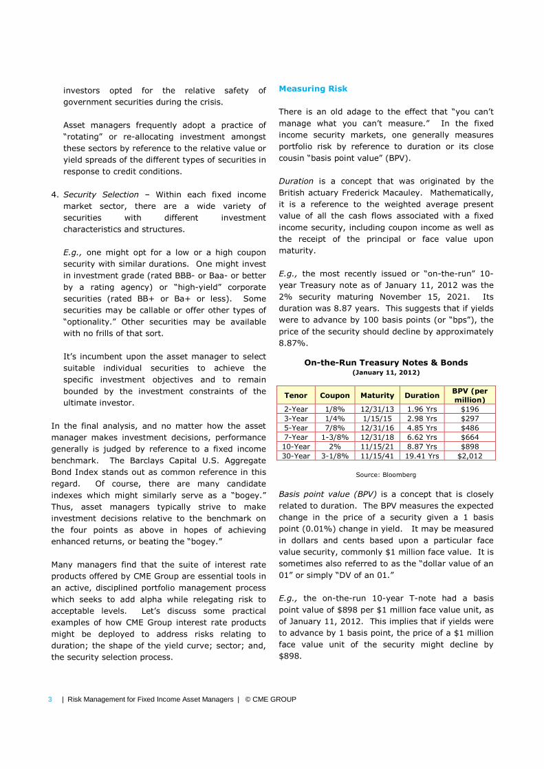
E.g., the most recently issued or “on-the-run” 10-
year Treasury note as of January 11, 2012 was the
2% security maturing November 15, 2021. Its
duration was 8.87 years. This suggests that if yields
were to advance by 100 basis points (or “bps”), the
price of the security should decline by approximately
8.87%.
On-the-Run Treasury Notes & Bonds (January 11, 2012)
Tenor Coupon Maturity Duration BPV (per
million)
2-Year 1/8% 12/31/13 1.96 Yrs $196
3-Year 1/4% 1/15/15 2.98 Yrs $297
5-Year 7/8% 12/31/16 4.85 Yrs $486
7-Year 1-3/8% 12/31/18 6.62 Yrs $664
10-Year 2% 11/15/21 8.87 Yrs $898
30-Year 3-1/8% 11/15/41 19.41 Yrs $2,012
Source: Bloomberg
Basis point value (BPV) is a concept that is closely
related to duration. The BPV measures the expected
change in the price of a security given a 1 basis
point (0.01%) change in yield. It may be measured
in dollars and cents based upon a particular face
value security, commonly $1 million face value. It is
sometimes also referred to as the “dollar value of an
01” or simply “DV of an 01.”
E.g., the on-the-run 10-year T-note had a basis
point value of $898 per $1 million face value unit, as
of January 11, 2012. This implies that if yields were
to advance by 1 basis point, the price of a $1 million
face value unit of the security might decline by
$898.
Page 4
4 | Risk Management for Fixed Income Asset Managers | © CME GROUP
Breakeven Risk Analysis
While we may attempt to measure the risks
associated with a specific Treasury security, we may
also attempt to identify the risks associated with
Treasury portfolios in general. One method for
assessing risk is to conduct what is known as a
“breakeven (B/E) rate analysis.” This technique
addresses the questions – how much do rates need
to advance before suffers a loss by holding a
particular security?
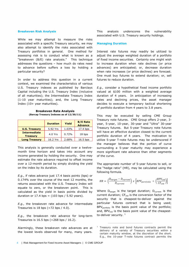
In order to address this question in a current
context, we examined the characteristics of various
U.S. Treasury indexes as published by Barclays
Capital including the U.S. Treasury Index (inclusive
of all maturities); the Intermediate Treasury Index
(1-10 year maturities); and, the Long Treasury
Index (10+ year maturities).
Breakeven Rate Analysis (Barcap Treasury Indexes as of 12/30/11)
Duration Yield B/E Rate
Advance
U.S. Treasury 5.92 Yrs 1.03% 17.4 bps
Intermediate
Treasury 4.0 Yrs 0.72% 18 bps
Long Treasury 16.2 Yrs 2.68% 16.5 bps
This analysis is generally conducted over a twelve-
month time horizon and takes into account any
income generated by holding the security. One may
estimate the rate advance required to offset income
over a 12-month period by simply dividing the yield
on the index by its duration.
E.g., if rates advance just 17.4 basis points (bps) or
0.174% over the course of the next 12 months, the
returns associated with the U.S. Treasury Index will
equate to zero, or the breakeven point. This is
calculated as the yield in basis points divided by
duration or 17.4 bps = (103 bps / 5.92 years).
E.g., the breakeven rate advance for intermediate
Treasuries is 18 bps (=72 bps / 4.0).
E.g., the breakeven rate advance for long-term
Treasuries is 16.5 bps (=268 bps / 16.2).
Alarmingly, these breakeven rate advances are at
the lowest levels observed for many, many years.
This analysis underscores the vulnerability
associated with U.S. Treasury security holdings.
Managing Duration
Interest rate futures may readily be utilized to
adjust the average weighted duration of a portfolio
of fixed income securities. Certainly one might wish
to increase duration when rate declines (or price
advances) are anticipated; or, decrease duration
when rate increases (or price declines) are forecast.
One must buy futures to extend duration; or, sell
futures to reduce duration.
E.g., consider a hypothetical fixed income portfolio
valued at $100 million with a weighted average
duration of 4 years. In anticipation of increasing
rates and declining prices, the asset manager
decides to execute a temporary tactical shortening
of portfolio duration from 4 years to 3.8 years.
This may be executed by selling CME Group
Treasury note futures. CME Group offers 2-year, 3-
year, 5-year, 10-year, 30-year and “Ultra” 30-year
Treasury futures. But 5-year Treasury note futures
will have an effective duration closest to the current
portfolio duration of 4 years. The motivation to
utilize 5-year T-note futures may be underscored if
the manager believes that the portion of curve
surrounding a 5-year maturity may experience a
more significant rate advance than other segments
of the curve.
The appropriate number of 5-year futures to sell, or
the “hedge ratio” (HR), may be calculated using the
following formula.
�� = ������ − � ����� ���� � � ������������ ÷���� ���� �� ��
Where Dtarget is the target duration; Dcurrent is the
current duration; CFctd is the conversion factor of the
security that is cheapest-to-deliver against the
particular futures contract that is being used;
BPVportfolio is the basis point value of the portfolio;
and, BPVctd is the basis point value of the cheapest-
to-deliver security. 1
1 Treasury note and bond futures contracts permit the
delivery of a variety of Treasury securities within a
certain maturity window, at the discretion of the short.
E.g., the 10-year T-note futures contract permits the
Page 5
5 | Risk Management for Fixed Income Asset Managers | © CME GROUP
E.g., assume that the $100 million portfolio had a
BPV equal to $40,000. As of January 11, 2012, the
cheapest-to-deliver (CTD) security against March
2012 5-year T-note futures was the 1-3/4% coupon
security maturing on May 15, 2016. The 1-3/4%-16
note had a conversion factor (CF) of 0.8453 with a
BPV of $44.25 per a $100,000 face value unit,
corresponding to the deliverable quantity against a
single futures contract.2 Using these inputs, the
appropriate hedge ratio may be calculated as short
38 futures contracts.
�� = �3.8 − 44 � � $$40,000 ÷($44.250.8453+, = −38
= -.//38�0102.3�45126713
By selling 38 Five-year T-note futures against the
portfolio, the asset manager may be successful in
pushing his risk exposure as measured by duration
from 4 to 3.8 years.
delivery of T-notes with a remaining maturity between 6-
1/2 to 10 years. This includes a rather wide variety of
securities with varying coupons and terms until maturity.
Because these securities may be valued at various
levels, the contract utilized a Conversion Factor (CF)
invoicing system to determine the price paid by long to
compensate the short for the delivery of the specific
security. Specifically, the principal invoice amount paid
from long to short upon delivery of securities is
calculated as a function of the futures price multiplied by
the CF. Technically, CFs are calculated as the price of
the particular security as if they were yielding the
“futures contract standard” of 6%. The system is
intended to render equally economic the delivery of any
eligible for delivery security. However, the mathematics
of the CF system is such that a single security tends to
stand out as most economic or cheapest-to-deliver
(CTD) in light of the relationship between the invoice
price of the security vs. the current market price of the
security. Typically, long duration securities are CTD
when prevailing yields are in excess of the 6% futures
market standard; while short duration securities are CTD
when prevailing yields are less than 6%. It is important
to identify the CTD security because futures will tend to
price or track or correlate most closely with the CTD. 2 These relationships are in fact dynamic and subject to
constant change. In particular, the BPV associated with any portfolio or security will change of its own accord in response to fluctuating yield levels. As a general rule, an asset holder might wish to review the structure of a hedge transaction upon a 20 basis point movement in prevailing yields. Further, the CTD will change as a function of changing yield levels, particularly when prevailing yields are in the vicinity of the 6% futures contract standard which may be regarded as an inflection point of sorts. However, this information may readily be obtained with use of a Bloomberg device or by navigating to the www.cmegroup.com website.
Sell 38 Five-year
T-note futures �
Reduces portfolio
duration from
4.0 to 3.8 years
If yields advance by 100 bps, the value of the
adjusted portfolio may decline by approximately
3.8% or $3.8 million. But this is preferable to a
possible $4 million decline in value if the asset
manager maintained the portfolio duration at the
original benchmark duration of 4 years. Thus, the
asset manager preserved $200,000 in portfolio
value. Or, viewed from the perspective of the client,
the asset manager successfully generated 20 bps
(0.20%) in alpha relative to the performance bogey,
which we assume maintains a static 4-year duration
for purposes of this example.
Of course, the asset manager may readily
accomplish the same objective simply by selling off a
portion of the portfolio holdings in favor of cash.
But Treasury futures tend to be more liquid than the
cash markets. Moreover, the futures hedge allows
the asset manager to maintain his current holdings
while adjusting duration exposures quickly and at
minimal costs.
Managing Yield Curve Exposure
Just as an asset manager may utilize interest rate
futures to adjust the effective duration of a portfolio,
in anticipation of fluctuating yield levels, interest
rate futures also provide utility in preserving or
enhancing value as a result of the dynamic shape of
the yield curve.
E.g., as of January 11, 2012, the 10-year on-the-run
(OTR) T-note was trading to yield 1.905% while the
2-year OTR T-note was at 0.229%. Thus, the 10-2
year yield spread was 168 bps (=1.905% less
0.229%). This yield spread had declined sharply
over the past year as a response to generally weak
economic conditions and driven further by the Fed’s
current version of Operation Twist announced in
September 2011. But assume that an asset
manager believes that this spread may advance as
the yield curve reverses to steepen once again.
Let’s consider the scenario that may inspire a
steepening yield curve. First, assume that the FOMC
adheres to its policy statement of August 9, 2011
when it announced it will maintain current rates until
mid 2013. Secondly, let’s assume that economy
Page 6
6 | Risk Management for Fixed Income Asset Managers | © CME GROUP
continues in its (early and mild) improvement,
highlighted by declining unemployment, growing
GDP and creeping inflationary pressures.
With the short-end of the curve anchored by Fed
monetary policy and the long-end of the curve
reacting to potential growth and inflationary
pressures, it is readily conceivable to witness a
steepening yield curve.
Let us further assume that the asset manager’s
Treasury holdings are structured to reflect a
benchmark or bogey against which investment
performance may be measured. As such, the
current portfolio duration may represent a carefully
targeted risk exposure that the portfolio manager
may wish to maintain. Still the prospect of a shift in
the yield curve may represent an opportunity that
an astute investment manager may view as an
opportunity to enhance returns, or to create “alpha”
per current investment vernacular.
CME Group Treasury futures may readily be utilized
to enhance investment returns based on an
expectation of a steeping yield curve (or a flattening
yield curve as well). Specifically, one may “buy the
curve” or buying 2-year and selling 10-year T-note
futures on a duration-balanced basis.
The key to capitalizing on the changing shape of the
yield curve is to use a “spread ratio” (SR) that
balances the effective duration of each futures
contract. By balancing the outright risk exposure,
as measured by BPV in each leg of the spread, one
can be reasonably assured that the spread will be
responsive only to the changing shape of the yield
and not to outright yield movements. As such, an
asset manager may enhance performance in
anticipation of a dynamic yield curve shape without
affecting the original portfolio duration.
-� = ���89:;�����<���=:;�����<
Where BPV10-yr futures is the effective basis point value
of the 10-year T-note futures contract; and, BPV2-yr
futures is the effective basis point value of the 2-year
T-note futures contract.
The effective BPV of a Treasury futures contract
(BPVfutures) may be found using the following
formula.
��������< =��� ���� ��
Where BPVctd is the basis point value of the
cheapest-to-deliver security against that futures
contract; and, CFctd is the conversion factor
associated with the cheapest-to-deliver security.3
E.g., as of January 11, 2012, the CTD security
against the March 2012 Ten-year T-note futures
contract was the 3-3/4% note maturing November
15, 2018. This security had a BPV of $71.23 per
$100,000 face value contract and a CF of 0.8804.
Thus, the BPV of the 10-year T-note futures contract
may be calculated as $80.91.
���89:;�����< = $71.230.8804 = $80.91
E.g., the CTD security against the March 2012 Two-
year T-note futures contract was the 1-1/2% note
maturing December 31, 2013. This security had a
BPV of $39.86 per $200,000 face value contract and
a CF of 0.9263. 4 Thus, the BPV of the 2-year T-
note futures contract may be calculated as $43.03.
���=:;�����< = $39.860.9263 = $43.03
E.g., plugging this data into our formula, we arrive
at a value of 1.880. This suggests for every Ten-
year futures contract that is sold, 1.880 Two-year
contracts should be purchased. 5
3 As discussed above, Treasury futures tend to price, track
or correlate most closely with the cheapest-to-deliver
(CTD) security. Thus, it is important to identify the CTD
security as the key to managing a hedging transaction.
Note that the CTD security is typically not found in the
on-the-run (OTR) security. 4 Most CME Group Treasury futures call for the delivery of
$100,000 face value in Treasuries. However, the 2-
Year T-note futures contract calls for the delivery of a
$200,000 face value unit. 5 It is, of course, not possible to transact fractional
futures contracts. Thus, one might buy the spread on a
ratio of 19:10 (1.90=19 ÷ 10); or, buy nineteen (19) 2-
year T-note futures; and, sell ten (10) 10-year T-note
futures. A 19:10 ratio should be effective in
neutralizing the spread to a parallel shift in the yield
curve. Consider that, if rates decline by one (1) basis
point, 19 long 2-year T-note futures should generate a
return of profit of $818 (=19 contracts x $43.03); while
10 short 10-year T-note futures should generate an
offsetting loss of $809 (=10 contracts x $80.91). Thus,
the two positions offset in the event of a parallel shift in
the curve.
Page 7
7 | Risk Management for Fixed Income Asset Managers | © CME GROUP
-� = $80.91$43.03 = 1.880
How much of this spread should the portfolio
manager transact? This decision is contingent upon
the investor’s view of potential spread movement;
and, risk tolerance relative to the benchmark.
E.g., assume that the portfolio manager believes the
yield curve spread between 10-year and 2-year
Treasuries may steepen, or advance, by 30 bps. 6
The manager further determines to limit risk to no
more than $100,000 if the curve flattens by 30 bps.
Thus, the asset manager may sell 41 Ten-year
futures [=($100,000 ÷ 30) ÷ $80.91]; and, buy 77
Two-year futures (=1.880 x 41 contracts).
Buy 77 Two-year
T-note futures &
sell 41 Ten-year
T-note futures
�
“Buying the curve”
enhances yields if
curve steepens
Assume the yield curve steepens by 30 bps as 6- to
10-year Treasury yields rise 40 bps; and, 2-year
Treasury yields rise 10 bps.
This implies that the 41 short 10-year futures may
advance in value by roughly $132,692 (=41
contracts x 40 bps x $80.91). This further implies
that the 77 long 2-year futures will decline in value
by roughly $33,133 (=77 contracts x 10 bps x
$43.03). Thus, the spread advances in value by
$99,559 (=$132,692 - $33,133), adding roughly 10
bps of “alpha” to the $100 million portfolio relative
to the benchmark.
Sector Weighting Strategy
Fixed income asset managers will generally allocate
their funds across various fixed income market
sectors, including Treasuries, agencies, corporate,
municipal securities, mortgage backed securities
6 The cheapest to deliver (CTD) security against 10-year
T-note futures was the 3-3/4% note of November 2018,
as of January 11, 2012. As such, 10-year T-note
futures were pricing or tracking or correlating most
closely with a security with a maturity of just under 7
years. Thus, as a technical matter, the 10-year/2-year
T-note futures spread might be characterized as a
spread between 7- and 2-year Treasuries. But for
most practical purposes, we refer to it as a 10- vs. 2-
year spread.
(MBS), commercial mortgage backed securities
(CMBS) and other asset backed securities (ABS).
Some asset managers conform the composition of
the portfolio to match that of the benchmark or
bogey. This strategy assures that the performance
of the portfolio generally will parallel performance of
the benchmark.
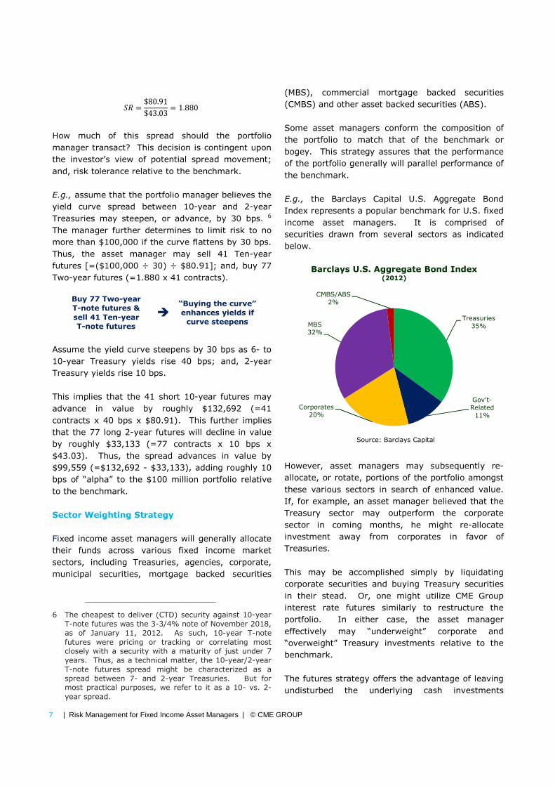
E.g., the Barclays Capital U.S. Aggregate Bond
Index represents a popular benchmark for U.S. fixed
income asset managers. It is comprised of
securities drawn from several sectors as indicated
below.
However, asset managers may subsequently re-
allocate, or rotate, portions of the portfolio amongst
these various sectors in search of enhanced value.
If, for example, an asset manager believed that the
Treasury sector may outperform the corporate
sector in coming months, he might re-allocate
investment away from corporates in favor of
Treasuries.
This may be accomplished simply by liquidating
corporate securities and buying Treasury securities
in their stead. Or, one might utilize CME Group
interest rate futures similarly to restructure the
portfolio. In either case, the asset manager
effectively may “underweight” corporate and
“overweight” Treasury investments relative to the
benchmark.
The futures strategy offers the advantage of leaving
undisturbed the underlying cash investments
Treasuries
35%
Gov't-
Related
11%
Corporates
20%
MBS
32%
CMBS/ABS
2%
Barclays U.S. Aggregate Bond Index(2012)
Source: Barclays Capital
Page 8
8 | Risk Management for Fixed Income Asset Managers | © CME GROUP
weighted according to the benchmark. Thus, this
may be referred to as an “overlay” strategy.
Further, CME Group futures generally offer superior
liquidity, i.e., you may generally transact more size
on tighter bid/ask spreads than may be possible in
the cash fixed income markets.
E.g., assume our asset manager with the $100
million portfolio with a duration of 4 years wished to
shift 10% of the portfolio from corporates into
Treasuries. As discussed above, the portfolio had an
aggregate BPV=$40,000. Thus, the transaction
should be constructed such that $4,000 (10% of
$40,000) in additional exposure, measured by BPV,
is allocated to Treasuries and away from corporates.
This may be accomplished by spreading Treasury
futures against Deliverable Swap Futures (DSF). 7
There are no viable corporate bond futures contracts
available. Thus, one may utilize CME Group
Deliverable Swap Futures (DSFs) as a reasonable
proxy for investment grade corporate risks, noting
that this implies some “basis risk.” In particular,
the correlations between 5-year IRS rates and
corporate bond yields are, while not perfect,
reasonably high. Still, some measure of basis risk is
implied in this strategy.
Correlation of Weekly Yield Fluctuations
of 5-Year Swap Rates vs. Corp Bond Yields
(Jan-05 thru Dec-11)
Bloomberg AAA 5-Year Industrials 0.7777
AA 5-Year Industrials 0.7938
A 5-Year Industrials 0.7545
BBB 5-Year Industrials 0.7484
The spread must be constructed such that an
equivalent risk exposure, measured by reference to
7 Deliverable Swap Futures (DSF) call for the delivery of
interest rate swap (IRS) instruments that are cleared and carried through the CME Clearing House facility. They are offered in several varieties that call for the delivery of $100,000 face value of 2-, 5-, 10- or 30-year IRS instruments. They are traded based upon an Exchange established coupon that is set near prevailing market rates, e.g., 0.5%, 1.0%, 1.5%, 2.0%, etc. Delivery occurs on the Monday prior to the 3rd Wednesday in the contract months of March, June, September and December. They are quoted as 100% of par plus the Non-Par Value (NPV) of the delivered swap. The final NPV of the futures contract is paid upon delivery of the IRS as it is booked in the Clearing House.
BPV, is bought and sold on each leg of the spread.
First, we must identify the BPV associated with each
futures contract.
E.g., the CTD security into the March 2013 10-year
Treasury note contract was the 3-3/8%-19 with a
BPV=$72.90 per $100,000 face value and a
CF=0.8604. Thus, the futures contract had an
effective BPV = $84.73 per $100,000 face value
(=$72.90/0.8604), as of 11/28/12. A (hypothetical)
10-year DSF contract with a 2% coupon has a BPV =
$99.21. 8
This suggests one may construct a spread on a ratio
of 1 Treasury per 0.85 DSFs (=$84.73/$99.21). To
the extent that the portfolio manager wishes to shift
10% of the portfolio or $4,000 in duration, this
requires 47 10-year T-note futures (=
$4,000/$84.73). A position of 47 long 10-year T-
note futures may be matched with the 40 short 10-
year DSFs (=0.85 x 47).
Buy 47 Ten-year
Treasury futures
& sell 40 Ten-year
DSF futures
�
Effectively rotates
10% of portfolio
from corporates to
Treasuries
If Treasury yields decline relative to swaps by 10
basis points, i.e., Treasuries outperform swaps, this
strategy may effectively enhance portfolio
performance by 4 basis points [=($84.73 x 10 basis
points x 47 contracts) / $100MM].
Selecting Securities
Sometimes opportunities in cash fixed income
markets are limited by the availability or
unavailability of certain investment structures.
Callable bonds offer a good example. Despite the
tremendous increase in the amount of Treasury
securities issued in recent years, the Treasury does
not currently issue callable securities. Since 2008,
the availability of callable U.S. agency securities has
similarly become limited. But callables may be
attractive investments, particular in low yield
environments to the extent that they offer a
premium yield to entice investors.
8 Note that DSFs were not launched until December
2012.
Page 9
9 | Risk Management for Fixed Income Asset Managers | © CME GROUP
Options on Treasury futures contracts may be
utilized synthetically to transform a Treasury
security holding into a callable security. To
understand, consider that when one purchases a
callable security, you effectively convey the right to
retire the security to the issuer. That right is likely
to be exercised if yields should decline as prices
advance. Thus, the call feature of a security may be
considered analogous to the sale of a call option.
Thus, let us consider the sale of call options as a
means of altering the risk/reward profile of a fixed
income portfolio. Further, let us consider the
purchase of puts as a form of “price insurance.”
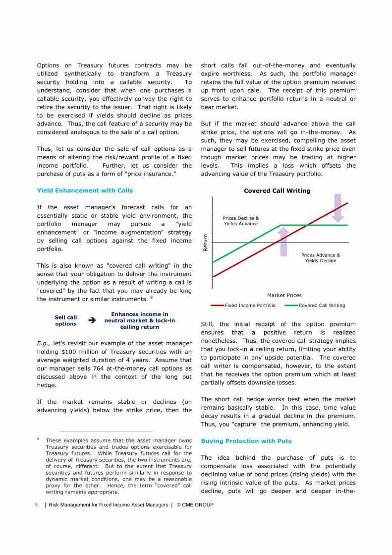
Yield Enhancement with Calls
If the asset manager’s forecast calls for an
essentially static or stable yield environment, the
portfolio manager may pursue a "yield
enhancement" or "income augmentation" strategy
by selling call options against the fixed income
portfolio.
This is also known as "covered call writing" in the
sense that your obligation to deliver the instrument
underlying the option as a result of writing a call is
"covered" by the fact that you may already be long
the instrument or similar instruments. 9
Sell call
options �
Enhances income in
neutral market & lock-in
ceiling return
E.g., let’s revisit our example of the asset manager
holding $100 million of Treasury securities with an
average weighted duration of 4 years. Assume that
our manager sells 764 at-the-money call options as
discussed above in the context of the long put
hedge.
If the market remains stable or declines (on
advancing yields) below the strike price, then the
9 These examples assume that the asset manager owns
Treasury securities and trades options exercisable for
Treasury futures. While Treasury futures call for the
delivery of Treasury securities, the two instruments are,
of course, different. But to the extent that Treasury
securities and futures perform similarly in response to
dynamic market conditions, one may be a reasonable
proxy for the other. Hence, the term “covered” call
writing remains appropriate.
short calls fall out-of-the-money and eventually
expire worthless. As such, the portfolio manager
retains the full value of the option premium received
up front upon sale. The receipt of this premium
serves to enhance portfolio returns in a neutral or
bear market.
But if the market should advance above the call
strike price, the options will go in-the-money. As
such, they may be exercised, compelling the asset
manager to sell futures at the fixed strike price even
though market prices may be trading at higher
levels. This implies a loss which offsets the
advancing value of the Treasury portfolio.
Still, the initial receipt of the option premium
ensures that a positive return is realized
nonetheless. Thus, the covered call strategy implies
that you lock-in a ceiling return, limiting your ability
to participate in any upside potential. The covered
call writer is compensated, however, to the extent
that he receives the option premium which at least
partially offsets downside losses.
The short call hedge works best when the market
remains basically stable. In this case, time value
decay results in a gradual decline in the premium.
Thus, you "capture" the premium, enhancing yield.
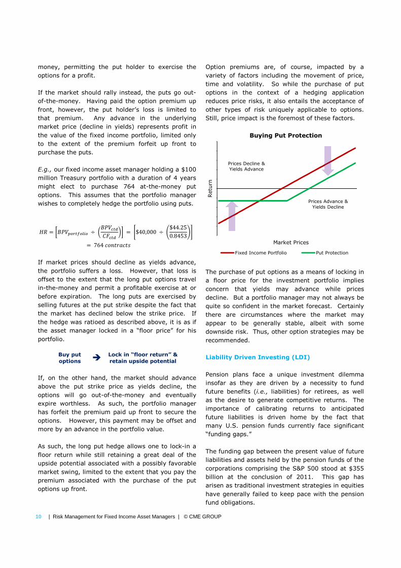
Buying Protection with Puts
The idea behind the purchase of puts is to
compensate loss associated with the potentially
declining value of bond prices (rising yields) with the
rising intrinsic value of the puts. As market prices
decline, puts will go deeper and deeper in-the-
-25.00
-20.00
-15.00
-10.00
-5.00
0.00
5.00
10.00
15.00
20.00
25.00
80
81
82
83
84
85
86
87
88
89
90
91
92
93
94
95
96
97
98
99
100
101
102
103
104
105
106
107
108
109
110
111
112
113
114
115
116
117
118
119
120
Retu
rn
Market Prices
Covered Call Writing
Fixed Income Portfolio Covered Call Writing
Prices Decline &
Yields Advance
Prices Advance &
Yields Decline
Page 10
10 | Risk Management for Fixed Income Asset Managers | © CME GROUP
money, permitting the put holder to exercise the
options for a profit.
If the market should rally instead, the puts go out-
of-the-money. Having paid the option premium up
front, however, the put holder’s loss is limited to
that premium. Any advance in the underlying
market price (decline in yields) represents profit in
the value of the fixed income portfolio, limited only
to the extent of the premium forfeit up front to
purchase the puts.
E.g., our fixed income asset manager holding a $100
million Treasury portfolio with a duration of 4 years
might elect to purchase 764 at-the-money put
options. This assumes that the portfolio manager
wishes to completely hedge the portfolio using puts.
�� = ������������ ÷ ���� ���� �� �� = $$40,000 �($44.250.8453+, � 764745126713
If market prices should decline as yields advance,
the portfolio suffers a loss. However, that loss is
offset to the extent that the long put options travel
in-the-money and permit a profitable exercise at or
before expiration. The long puts are exercised by
selling futures at the put strike despite the fact that
the market has declined below the strike price. If
the hedge was ratioed as described above, it is as if
the asset manager locked in a “floor price” for his
portfolio.
Buy put
options � Lock in “floor return” &
retain upside potential
If, on the other hand, the market should advance
above the put strike price as yields decline, the
options will go out-of-the-money and eventually
expire worthless. As such, the portfolio manager
has forfeit the premium paid up front to secure the
options. However, this payment may be offset and
more by an advance in the portfolio value.
As such, the long put hedge allows one to lock-in a
floor return while still retaining a great deal of the
upside potential associated with a possibly favorable
market swing, limited to the extent that you pay the
premium associated with the purchase of the put
options up front.
Option premiums are, of course, impacted by a
variety of factors including the movement of price,
time and volatility. So while the purchase of put
options in the context of a hedging application
reduces price risks, it also entails the acceptance of
other types of risk uniquely applicable to options.
Still, price impact is the foremost of these factors.
The purchase of put options as a means of locking in
a floor price for the investment portfolio implies
concern that yields may advance while prices
decline. But a portfolio manager may not always be
quite so confident in the market forecast. Certainly
there are circumstances where the market may
appear to be generally stable, albeit with some
downside risk. Thus, other option strategies may be
recommended.
Liability Driven Investing (LDI)
Pension plans face a unique investment dilemma
insofar as they are driven by a necessity to fund
future benefits (i.e., liabilities) for retirees, as well
as the desire to generate competitive returns. The
importance of calibrating returns to anticipated
future liabilities is driven home by the fact that
many U.S. pension funds currently face significant
“funding gaps.”
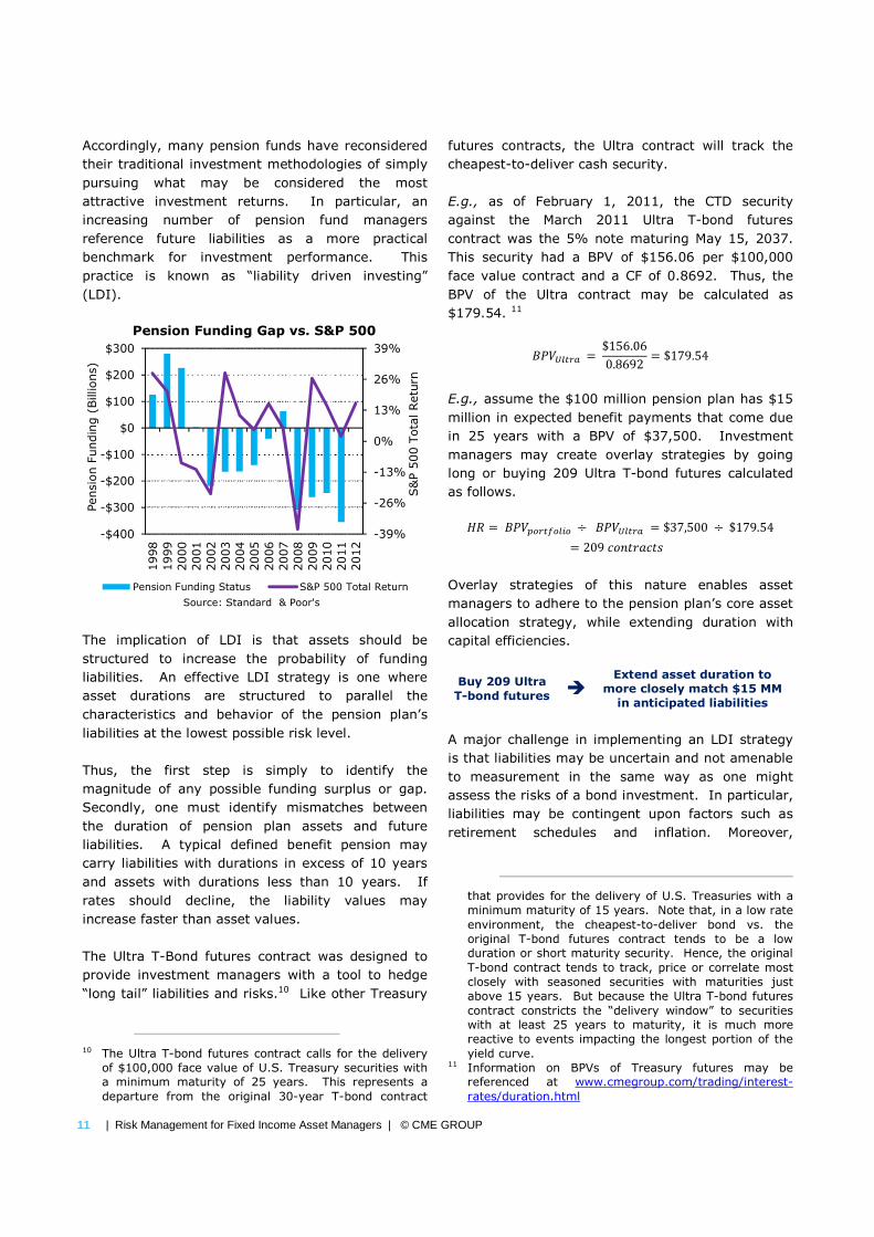
The funding gap between the present value of future
liabilities and assets held by the pension funds of the
corporations comprising the S&P 500 stood at $355
billion at the conclusion of 2011. This gap has
arisen as traditional investment strategies in equities
have generally failed to keep pace with the pension
fund obligations.
-25.00
-20.00
-15.00
-10.00
-5.00
0.00
5.00
10.00
15.00
20.00
25.00
80
81
82
83
84
85
86
87
88
89
90
91
92
93
94
95
96
97
98
99
100
101
102
103
104
105
106
107
108
109
110
111
112
113
114
115
116
117
118
119
120
Retu
rn
Market Prices
Buying Put Protection
Fixed Income Portfolio Put Protection
Prices Decline &
Yields Advance
Prices Advance &
Yields Decline
Page 11
11 | Risk Management for Fixed Income Asset Managers | © CME GROUP
Accordingly, many pension funds have reconsidered
their traditional investment methodologies of simply
pursuing what may be considered the most
attractive investment returns. In particular, an
increasing number of pension fund managers
reference future liabilities as a more practical
benchmark for investment performance. This
practice is known as “liability driven investing”
(LDI).
The implication of LDI is that assets should be
structured to increase the probability of funding
liabilities. An effective LDI strategy is one where
asset durations are structured to parallel the
characteristics and behavior of the pension plan’s
liabilities at the lowest possible risk level.
Thus, the first step is simply to identify the
magnitude of any possible funding surplus or gap.
Secondly, one must identify mismatches between
the duration of pension plan assets and future
liabilities. A typical defined benefit pension may
carry liabilities with durations in excess of 10 years
and assets with durations less than 10 years. If
rates should decline, the liability values may
increase faster than asset values.
The Ultra T-Bond futures contract was designed to
provide investment managers with a tool to hedge
“long tail” liabilities and risks.10 Like other Treasury
10 The Ultra T-bond futures contract calls for the delivery
of $100,000 face value of U.S. Treasury securities with
a minimum maturity of 25 years. This represents a
departure from the original 30-year T-bond contract
futures contracts, the Ultra contract will track the
cheapest-to-deliver cash security.
E.g., as of February 1, 2011, the CTD security
against the March 2011 Ultra T-bond futures
contract was the 5% note maturing May 15, 2037.
This security had a BPV of $156.06 per $100,000
face value contract and a CF of 0.8692. Thus, the
BPV of the Ultra contract may be calculated as
$179.54. 11
���B��� �$156.060.8692 = $179.54
E.g., assume the $100 million pension plan has $15
million in expected benefit payments that come due
in 25 years with a BPV of $37,500. Investment
managers may create overlay strategies by going
long or buying 209 Ultra T-bond futures calculated
as follows.
�� = ����������� ÷ ���B��� = $37,500 ÷ $179.54= 209745126713
Overlay strategies of this nature enables asset
managers to adhere to the pension plan’s core asset
allocation strategy, while extending duration with
capital efficiencies.
Buy 209 Ultra
T-bond futures �
Extend asset duration to
more closely match $15 MM
in anticipated liabilities
A major challenge in implementing an LDI strategy
is that liabilities may be uncertain and not amenable
to measurement in the same way as one might
assess the risks of a bond investment. In particular,
liabilities may be contingent upon factors such as
retirement schedules and inflation. Moreover,
that provides for the delivery of U.S. Treasuries with a
minimum maturity of 15 years. Note that, in a low rate
environment, the cheapest-to-deliver bond vs. the
original T-bond futures contract tends to be a low
duration or short maturity security. Hence, the original
T-bond contract tends to track, price or correlate most
closely with seasoned securities with maturities just
above 15 years. But because the Ultra T-bond futures
contract constricts the “delivery window” to securities
with at least 25 years to maturity, it is much more
reactive to events impacting the longest portion of the
yield curve. 11 Information on BPVs of Treasury futures may be
referenced at www.cmegroup.com/trading/interest-
rates/duration.html
-39%
-26%
-13%
0%
13%
26%
39%
-$400
-$300
-$200
-$100
$0
$100
$200
$300
1998
1999
2000
2001
2002
2003
2004
2005
2006
2007
2008
2009
2010
2011
2012
S&
P 5
00 T
ota
l Retu
rn
Pensio
n F
undin
g (
Billions)
Pension Funding Gap vs. S&P 500
Pension Funding Status S&P 500 Total Return
Source: Standard & Poor's
Page 12
12 | Risk Management for Fixed Income Asset Managers | © CME GROUP
liabilities are marked to market based on corporate
yield curves which are not directly investable in the
cash, futures or over the counter derivative markets.
As such, a certain level of basis risk will be inherent
in any strategy.
Pension plan managers faced with a deficit position
are further faced with the dilemma of deciding when
to “lock-in” prevailing interest rates. Instead of
simply buying futures at current rates, they may opt
to sell out-of-the-money (OTM) put options on
Treasury futures.
This strategy represents an effective way of
providing for possible yield enhancement without
locking in low interest rates. Often, this strategy is
pursued on a “scalable” basis. In particular, the sale
of OTM puts allows the asset manager to establish
target rates at which they might extend portfolio
duration to more closely match liability durations.
Conclusion
CME Group is committed to finding effective and
practical risk-management solutions for fixed income
asset managers in a dynamic economic
environment. While the recent financial crisis has
sent shivers through the investment community, it is
noteworthy that CME Group performed flawlessly
throughout these trying times. Our products offer
deep liquidity, unmatched financial integrity and
innovative solutions to risk management issues.
Copyright 2013 CME Group All Rights Reserved. Futures trading is not suitable for all investors, and involves the risk of loss. Futures
are a leveraged investment, and because only a percentage of a contract’s value is required to trade, it is possible to lose more than the
amount of money deposited for a futures position. Therefore, traders should only use funds that they can afford to lose without affecting
their lifestyles. And only a portion of those funds should be devoted to any one trade because they cannot expect to profit on every
trade. All examples in this brochure are hypothetical situations, used for explanation purposes only, and should not be considered
investment advice or the results of actual market experience.”
Swaps trading is not suitable for all investors, involves the risk of loss and should only be undertaken by investors who are ECPs within the
meaning of section 1(a)18 of the Commodity Exchange Act. Swaps are a leveraged investment, and because only a percentage of a
contract’s value is required to trade, it is possible to lose more than the amount of money deposited for a swaps position. Therefore, traders
should only use funds that they can afford to lose without affecting their lifestyles. And only a portion of those funds should be devoted to
any one trade because they cannot expect to profit on every trade.
CME Group is a trademark of CME Group Inc. The Globe logo, E-mini, Globex, CME and Chicago Mercantile Exchange are trademarks of
Chicago Mercantile Exchange Inc. Chicago Board of Trade is a trademark of the Board of Trade of the City of Chicago, Inc. NYMEX is a
trademark of the New York Mercantile Exchange, Inc.
The information within this document has been compiled by CME Group for general purposes only and has not taken into account the
specific situations of any recipients of the information. CME Group assumes no responsibility for any errors or omissions. Additionally, all
examples contained herein are hypothetical situations, used for explanation purposes only, and should not be considered investment advice
or the results of actual market experience. All matters pertaining to rules and specifications herein are made subject to and are superseded
by official CME, NYMEX and CBOT rules. Current CME/CBOT/NYMEX rules should be consulted in all cases before taking any action.