Risk-neutral modelling with affine and non-affine models

Garland B. Durham∗

October 10, 2012

Abstract

Option prices provide a great deal of information regarding the market’s expec-tations of future asset price dynamics. But, the implied dynamics are under therisk-neutral measure rather than the physical measure under which the price ofthe underlying asset itself evolves. This paper demonstrates new techniques forjoint analysis of the physical and risk-neutral models using data from both theunderlying asset and options. While much of the prior work in this area hasfocused on affine and affine-jump models because of their analytical tractability,the techniques used in this paper are straightforward to apply to a broad classof models of potential interest. The techniques are based on evaluating variousintegrals of interest using Monte Carlo sums over simulated volatility paths. In anapplication using S&P 500 index data, we find that log volatility models performdramatically better than affine models, but that some evidence of misspecificationremains.

∗Leeds School of Business, University of Colorado at Boulder, 419 UCB, Boulder, CO 80309-0419; email: garland.durham@colorado.edu.

1 Introduction

Option prices provide a great deal of information regarding the market’s expec-

tations of future asset price dynamics. But, the implied dynamics are under the

risk-neutral measure rather than the physical measure under which the price of the

underlying asset itself evolves.

This paper demonstrates new techniques for joint analysis of the physical and

risk-neutral models using data from both the underlying asset and options. While

much of the prior work in this area has focused on affine and affine-jump models

because of their analytical tractability, the techniques used in this paper are straight-

forward to apply to a broad class of models of potential interest. The techniques

are based on evaluating various integrals of interest using Monte Carlo sums over

simulated volatility paths. Although simulation-based techniques are often compu-

tationally intensive, the approach demonstrated in this paper run in a few minutes

on a typical desktop computer.

Understanding the dynamics of returns and volatility and the relationship be-

tween physical and risk-neutral measures are all fundamental issues in asset pricing.

A better understanding of these issues can provide useful information regarding

risk premia and help in the development of effective risk-management and hedging

strategies.

The modeling framework is based on a class of stochastic volatility models

which include the possibility of jumps in both returns and volatility. In the empirical

section, we examine log volatility and affine models with various jump specifications.

We provide maximum likelihood estimates for the physical and risk-neutral models

and useful diagnostics based on generalized residuals. Although this is not novel for

2

affine models (e.g., Eraker 2004), the methods proposed in this paper are important

because they can be applied to log volatility models as well, including models with

jumps in both returns and volatility.

The application uses daily observations of the S&P 500 (SPX) and VIX indices

over the period Jan 2, 1990 - Dec 29, 2006 (n=4284). The VIX is designed to

replicate a model-free measure of expected integrated volatility (IV) based on work

by Britten-Jones and Neuberger (2000). Using the VIX as a proxy for IV, and

given a model and candidate parameter vector, it is possible to back out the latent

volatility states (under the risk-neutral measure). Given the time-series of implied

volatility states and observed SPX prices, the log likelihood of the model can be

computed (under the physical measure). Optimizing over the parameter space gives

the maximum likelihood estimator (MLE).

Since many of the models under consideration are not nested, testing using, e.g.,

likelihood ratio tests is not straightforward. However, model performance can still be

compared using information-based criteria such as the Akaike information criterion

(AIC) or Schwarz criterion (SC). In addition, we examine several diagnostics based

on generalized residuals. A useful feature is that the residuals can be decomposed

into return and volatility components. The analysis of these generalized residuals

proceeds along much the same lines as the residual analysis familiar from more

standard time-series models. Useful graphical tools include normal-quantile plots

and autocorrelation plots. Conventional model testing can be performed using, e.g.,

Jarque-Bera or Box-Pierce tests. These diagnostics provide a great deal of insight

into what aspects of the data the models are able to fit and where they fail.

Our results corroborate previous research which finds that including jumps

in returns provides a big improvement in model fit, and that including jumps in

3

volatility as well provides an additional large improvement. However, we find that

the best of the log volatility models is over 600 points in log likelihood better than

the best affine model. Indeed, the best of the affine models is nearly 300 points

worse than even the simplest log volatility model which includes jumps in neither

returns nor volatility.

The diagnostics also point to serious problems in the affine models. The square-

root specification for volatility of volatility does not reflect the data. Including

jumps helps but does not resolve this problem. Also, using exponentially distributed

jumps in volatility (as proposed by Duffie, Pan, and Singleton 2000) is problematic.

This specification implies that jumps are either always positive or always negative

(depending on the sign of the coefficient). But the data suggest that volatility can

jump in both directions. The fitted models do a good job of capturing large positive

moves in volatility, but fail to capture the large downward moves that are also

observed.

Log volatility models also have difficulty with some of the diagnostics, but

the defects are less severe. Although affine models are often used in applied work

due to their analytical tractability, the log volatility models provide a much better

description of the data.

There is a large body of related literature. A number of papers estimate the

physical model directly from returns without trying to make use of any additional

information on the volatility state. Jacquier, Polson, and Rossi (1994) demonstrate

computationally efficient Bayesian techniques, which involve MCMC techniques for

sampling over the latent state space. Jacquier, Polson, and Rossi (2004), Eraker

(2001), Eraker, Johannes, and Polson (2003), Shephard and Pitt (1997), Kim, Shep-

hard, and Chib (1998), Gallant and Tauchen (1996), Durbin and Koopman (1997),

4

Liesenfeld and Richard (2003), Bates (2006), and Durham (2006), among many oth-

ers have added to this literature. Andersen, Benzoni, and Lund (2002) and Chernov,

Gallant, Ghysels, and Tauchen (2003) provide comprehensive studies comparing a

number of models using a simulated method of moments approach.

However, there has also been a great deal of work toward trying to get infor-

mationally efficient proxies for the volatility state. Such proxies are of independent

interest as well as being useful in estimating models for asset returns. One partic-

ularly fruitful avenue of research is based on the idea of using high-frequency infor-

mation to get a proxy for the volatility state (e.g., Andersen, Bollerslev, Diebold,

and Labys 2003; Barndorff-Nielsen and Shephard 2002; Ghysels, Santa-Clara, and

Valkanov 2006; Garcia, Lewis, Pastorello, and Renault 2011). Theory suggests that

if the price process is a diffusion, then high frequency observations should provide

precise information as to the volatility state. In practice, there are some problems

that need to be addressed. Nonetheless, this approach shows great promise, as evi-

denced by the large body of recent work devoted to applications as well as further

development of the underlying theory.

An alternative is to use the information embedded in option prices to obtain

a proxy for the volatility state. The simplest way of doing so involves using Black-

Scholes implied volatility directly as a proxy. There are problems with this approach

due to the fact that volatility is time-varying and log return distributions are non-

Gaussian, contrary to the assumptions underlying the Black-Scholes pricing formula,

but corrections are available to address these issues to some extent (e.g., Bollerslev

and Zhou 2006). More problematic is the possible presence of risk premia in the

volatility dynamics. If such risk premia exist, then option prices will have differ-

ent implications for spot volatility under the physical and risk-neutral measures. If

5

this distinction is ignored, then option-implied spot volatility will be systematically

biased. Indeed, there is considerable evidence that this may be the case (e.g., Flem-

ing, Ostdiek, and Whaley 1995; Christensen and Prabhala 1998; Corrado and Miller

2005).

The approach taken in this paper uses option prices to back out implied volatil-

ity states with an explicitly specified risk-neutral measure and risk premia es-

timated from data. Previous work using this idea includes Pastorello, Renault,

and Touzi (2000), Chernov and Ghysels (2000), Pan (2002), Jones (2003), Eraker

(2004), Christoffersen, Jacobs, and Mimouni (2006), Broadie, Chernov, and Jo-

hannes (2007), among others. In theory, this approach should be capable of elimi-

nating the bias in implied volatility found in previous empirical work, while at the

same time providing direct evidence regarding risk premia. Also, since there is some

overlap of the physical and risk-neutral parameters, some have argued that more

informative parameter estimates for the physical model may be obtained in this

manner (because of the richness of option price data). However, the theory relies

heavily upon the assumption of correctly specified models.

This paper builds on existing work in several directions. First, we demonstrate

an efficient, simulation-based approach for inverting the risk-neutral measure to

obtain the spot volatility state from a panel of observed option prices. Secondly,

we demonstrate an efficient approach for maximum likelihood estimation using the

observed asset prices and implied volatility states. And finally, we provide a useful

set of diagnostics. The critical point is that, while much of the existing literature

uses affine and affine-jump models for computational tractability, the techniques

used in this paper are applicable to more general models, including log volatility

models that fit observed data much better.

6

This paper is organized as follows: Section 2 describes the class of models used,

Section 3 describes the methodology, Section 4 provides the application, and Section

5 concludes.

2 Models

The asset price dynamics are described by the model

dXt/Xt = [µX(Vt)− λ1µ1t] dt+ σX(Vt) dW1t + J1t dN1t

dVt = [µV (Vt)− λ2µ2t] dt+ σV (Vt) dW2t + J2t dN2t

where Xt is the asset price and Vt is the volatility state, W1t and W2t are Brownian

motions with correlation ρ, Nit is a Poisson process with intensity λi (i = 1, 2), and

µit = E(Jit) (i = 1, 2).

For computational purposes, it is often more convenient to work with the log

price process,

dYt = [µY (Vt)− λ1tµ1t] dt+ σY (Vt) dW1t + J1t dN1t

dVt = [µV (Vt)− λ2tµ2t] dt+ σV (Vt) dW2t + J2t dN2t

(1)

where Yt = log(Xt), µY = µX − .5σ2X , σY = σX and J1t = log(1 + J1t). For future

reference, also denote µ1t = E(J1t).

The probability measure P over which the model describing the dynamics of

observed asset prices is defined is commonly referred to as the objective or physical

measure. In order to compute option prices, we make use of an equivalent martingale

measure Q under which the discounted stock price, Xt = Xt exp[∫ t

0 (qτ − rτ ) dτ],

is a martingale, where qt is the dividend payout rate and rt is the risk-free interest

rate. Q is often referred to as the risk-neutral measure. The idea is that if any

7

derivative security with time T payoff H(XT ) is priced according to the risk-neutral

expectation

Pt = EQt

{H(XT ) exp

[∫ T

t(qτ − rτ ) dτ

]},

then there are no arbitrage opportunities (subject to some regularity conditions).

The risk neutral dynamics are given by

dXt/Xt = [µ∗X(Vt)− λ1tµ∗1t] dt+ σX(Vt) dW

∗1t + J∗1t dN1t

dVt = [µ∗V (Vt)− λ2tµ∗2t] dt+ σV (Vt) dW

∗2t + J∗2t dN2t

whereW ∗1 andW ∗2 are Brownian motions with correlation ρ underQ and E(J∗it) = µ∗it

(i = 1, 2). Similarly, the risk-neutral model for log prices is given by

dYt = [µ∗Y (Vt)− λ1tµ∗1t] dt+ σY (Vt) dW

∗1t + J∗1t dN1t

dVt = [µ∗V (Vt)− λ2tµ∗2t] dt+ σV (Vt) dW

∗2t + J∗2t dN2t

where µ∗Y = µ∗X − .5σ2X , J∗1t = log(1 + J∗1t) and everything else is as above.

The relationship between physical and risk-neutral measures is well-documented

(e.g., Fouque, Papanicolaou, and Sircar 2000; Lewis 2000; Romano and Touzi 1997).

There are two potential sources of risk premium: diffusive risk premia are determined

by the differences between µX(Vt) and µ∗X(Vt) and between µV (Vt) and µ∗V (Vt); and

jump risk premia are determined by the differences between Jit and J∗it (i = 1, 2).

The requirement that the discounted stock price be a martingale implies that µ∗X =

rt − qt. Given a particular specification for the physical and risk-neutral models

together with a set of estimated parameters, it is straightforward to back out the

implied market prices of risk corresponding to the various sources of uncertainty in

the model.

Both the risk-free rate, rt, and dividend payout rate, qt, are treated as deter-

ministic (but time-varying). While it would be straightforward to treat these as

8

varying randomly, the effect of doing so is negligible.

We examine two classes of models, log volatility and affine (see Table 1), with

several different specifications for jumps in each class.

For the log volatility models: we consider models with no jumps; jumps in

returns alone; and jumps in both returns and volatility. Return jumps are ei-

ther scaled by volatility or not. Let ξit ∼ N(µi, σ2i ) (i = 1, 2). For the mod-

els with unscaled jumps, the jump distribution does not depend on the volatil-

ity state and J1t = log(1 + J1t) = ξ1t, implying that µ1t = E(J1t) = µ1 and

µ1t = E(J1t) = exp(µ1 + .5σ21)− 1. For models with scaled jumps, Jt = exp(Vt/2)ξ1t

with corresponding changes in µ1t and µ1t. Jumps in volatility either occur at the

same time as jumps in returns and are correlated with them, or they are inde-

pendent of jumps in returns. In either case, J2t = ξ2t. In the case of correlated

jumps, N1 = N2 and corr(ξ1t, ξ2t) = ρJ . In the uncorrelated case, N1 6= N2 and

corr(ξ1t, ξ2t) = 0. Jump specifications under the risk-neutral measure are analagous

in each case.

To summarize, the log volatility models under consideration are:

Log No jumps.

LogJ0 Return jumps only, unscaled.

LogJ1 Return jumps only, scaled.

LogJJ0 Jumps in returns and volatility, correlated and unscaled.

LogJJ1 Jumps in returns and volatility, correlated and scaled.

LogJJ2 Jumps in returns and volatility, uncorrelated and unscaled.

LogJJ3 Jumps in returns and volatility, uncorrelated and scaled.

9

We consider an analogous collection of affine models. Let ξ1t ∼ N(µ1, σ21) and

ξ2t ∼ exp(1) be independent random variables. In the unscaled, uncorrelated case,

J1t = ξ1t and J2t = µ2ξ2t. In the unscaled, correlated case, J1t = ξ1t + ρJξ2t and

J2t = µ2ξ2t. The scaled cases are analogous, but J1t is scaled by a factor of√Vt.

To summarize, the affine models under consideration are:

Aff No jumps.

AffJ0 Return jumps only, unscaled.

AffJ1 Return jumps only, scaled.

AffJJ0 Jumps in returns and volatility, correlated and unscaled.

AffJJ1 Jumps in returns and volatility, correlated and scaled.

AffJJ2 Jumps in returns and volatility, uncorrelated and unscaled.

AffJJ3 Jumps in returns and volatility, uncorrelated and scaled.

AffJJ0 and AffJJ2 are essentially equivalent to the SVCJ and SVIJ models used

by Eraker, Johannes, and Polson (2003).

3 Methods

There are four steps involved in fitting and assessing the models under consideration:

• Given an observed panel of option prices at time t, invert the risk-neutral

measure to get the implied volatility state.

• Given time series of observed asset prices and implied volatility states, compute

the log likelihood of the data.

10

• Optimize over the parameter space to obtain the MLE.

• Examine some diagnostics.

The third step is straightforward. Gradients are computed numerically (the

likelihood surface is smooth in the parameters). Optimization can proceed using

Newton’s method with a Hessian computed either using finite differences or from

the outer-product of the gradient (OPG). Alternatively, a method such as BFGS

that does not require Hessians could be used. In either case, standard errors can

be obtained using a Hessian computed from the OPG. The candidate parameter

vectors include both physical and risk-neutral parameters; implied volatility states

are obtained by inverting the risk-neutral model at each evaluation of the likelihood

function. See Pastorello, Patilea, and Renault (2003) for an alternative iterative

approach.

We now address each of the other steps involved in the analysis in more detail.

The convention used throughout this paper will be to measure time in days. Data is

observed daily (weekends and holidays are ignored). Note that, in principle, there is

no need for the observation frequency to be constant. This convention is maintained

only for notational convenience.

3.1 Implied volatility

Britten-Jones and Neuberger (2000) show that for a broad class of diffusion models,

the risk-neutral expectation of the integrated variance of returns (IV hereafter)

11

between time t and time t+ ∆ can be computed from option prices:

EQt

[∫ t+∆

t

(dXτ

Xτ

)2

dτ

]

= 2

∫ ∞0

C(t+ ∆,K)/Bt(∆)−max(0, St/Bt(∆)−K)

K2dK

where C(t + ∆,K) is the price at time t of a European call option with maturity

t+ ∆ and strike price K and Bt(∆) is the time t price of a bond paying $1 at time

t + ∆. A similar expression can be constructed using put prices in place of call

prices. Jiang and Tian (2005) show that the expression above is approximately in

true in models including jumps.

Beginning in 2003, the CBOE began reporting a revised VIX index based on

implementing the right-hand side of the above expression using S&P 500 index

(SPX) options (they also provide historical data calculated using the same algorithm

going back to Jan. 2, 1990). SPX options are European, so there are no issues with

early exercise premia. A constant 30-day horizon is maintained by interpolating

between the integrated variances implied by options with the two shortest times

to maturity greater than 8 days. The exact construction can be looked up on the

CBOE web site. The quantity actually reported is the square root of the integrated

variance.

While the construction of the VIX index is intended to approximate the right

hand side of the above expression, there are only a finite number of strikes traded,

hence some approximation error is inevitable. The possible presence of jumps could

introduce some additional approximation error. On the other hand, evidence pro-

vided by Jiang and Tian suggests that the error is likely to be quite small in practice.

They argue that the VIX should provide a good proxy for the market’s risk neutral

expectation of the integrated volatility of returns.

12

While the VIX could potentially be used directly as a proxy for the spot volatil-

ity, it has been found to be a substantially biased forecaster of realized volatility.

By inverting the risk-neutral measure to get the spot volatility implied by the VIX

(as a proxy for expected integrated volatility), we hope that we can explain this bias

by a risk premium and get better forecasts of realized volatility.

The problem of how to obtain the value of the volatility state variable (and

thus spot volatility) given an observed value of IV remains. This is comparable to

the problem of inverting option prices to obtain spot volatility (e.g., Pan 2002).

The first step involves computing the IV corresponding to a given value of the

state variable. We solve this problem using simulation techniques similar to those

commonly used to compute option prices (e.g., Romano and Touzi 1997). Jiang and

Tian show that

EQt

[∫ t+∆

t

(dXτ

Xτ

)2

dτ

]≈ EQt

{∫ t+∆

t

[σ2Y (Vτ ) + λ1J

∗1τ

2]dτ

}.

(Note that if the model does not include jumps, the above expressions are exactly

equal; with jumps they are only approximately equal). Given an initial condition Vt,

it is straightforward to compute the right hand side expectation by means of Monte

Carlo techniques. Using the risk neutral model dynamics, simulate volatility paths

V(s)τ for τ ∈ [t, t+ ∆] and s = 1, . . . , S. Then, the expectation can be approximated

by

EQt

[∫ t+∆

t

(dXτ

Xτ

)2

dτ

]≈ 1

S

S∑s=1

{∫ t+∆

t

[σ2Y (V (s)

τ ) + λ1 E(J∗1τ2)]dτ

}.

In practice, paths are simulated using the Euler scheme with discretization τi = t+δi

for i = 0, . . . ,∆/δ, whence

EQt

[∫ t+∆

t

(dXτ

Xτ

)2

dτ

]≈ 1

S

S∑s=1

∆/δ−1∑i=0

[σ2Y (V (s)

τi ) + λ1 E(J∗1,τi2)]δ. (2)

13

But, what we actually need is the inverse of the mapping described above,

Γ : IVt → Vt.

That is, given an observed value of IVt, we need to obtain the implied volatility

state, Vt. This is accomplished using an interpolation scheme constructed as follows.

Choose a grid of values, V1, . . . , VG (the hats serve to distinguish grid points from

data observations). At each grid point, evaluate the integral as described above

in Equation (2) to get a collection of pairs {( ˆIV g, Vg), g = 1, . . . , G}. Now, we

use this collection of pairs as the basis for approximating the transformation Γ.

Many schemes for doing this are possible, including polynomials, splines, etc. In

this paper, we use a simple polynomial approximation scheme. A cubic polynomial,

Γ, is chosen to minimize∑G

g=1

[Γ( ˆIV g)− σY (Vg)

]2. Having found Γ, it is easy to

compute Vt = Γ(IVt) ≈ σ−1Y (Γ(IVt)) for any t. When computing the log likelihood,

we will also need to be able to compute the derivative of Γ. This is straightforward.

The preceding procedure could also be implemented for assets other than the

S&P 500 by constructing an expected integrated volatility series directly from option

prices in a manner analogous to the construction of the VIX. If options are not

European, the issue of early exercise premia must be dealt with.

One could also do something similar to the above procedure using option prices

directly, without going through the intermediate step of constructing the expected

integrated volatility. It is straightforward to compute the mapping from spot volatil-

ity to option prices using simulation methods. The inverse transformation can be

approximated using an interpolation scheme similar to that described above. Once

one has started down the road of averaging over simulated volatility paths, it does

not make much difference in principle whether those paths are used to compute

model-implied option prices or integrated volatility.

14

But there are several factors that motivate using the VIX index rather than

fitting option prices directly: it is less computationally costly to obtain the IV cor-

responding to a candidate value of the volatility state by simulating (2) than it is to

simulate panels of option prices; the issue of arbitrarily choosing either a particular

option price to match at each date or a weighting scheme for error minimization is

avoided; and the VIX is readily available, meaning that data issues are greatly sim-

plified. Using the VIX (or similar measures of option-implied volatility) makes doing

exercises of this nature a routine matter. In particular, our results can be easily

replicated by anyone interested in doing so. We believe that third-party replicability

of results is important.

3.2 Likelihood computation

Given observed series of log stock prices, Y = (Y1, . . . , Yn) and integrated volatility,

IV = (IV1, . . . , IVn), the goal is to compute the log likelihood, logL(Y, IV). In

practice, this is done using the identity

logL(Y, IV) =

n∑t=2

log p(Yt, IVt|Yt−1, IVt−1)

=n∑t=2

[log p(Yt, Vt|Yt−1, Vt−1) + log Γ′(IVt)

]where Γ′(IVt) is the Jacobian of the transformation from IVt to Vt under the risk-

neutral model and the conditional densities, p(Yt, Vt|Yt−1, Vt−1), are computed under

the physical measure. Note that the risk-neutral measure is inverted at each eval-

uation of the likelihood to obtain the latent volatility states Vt conditional on the

candidate parameter vector.

The problem is how to compute the conditional densities. In this paper, we use

an Euler scheme approximation. Given a discretization, τ0, τ1, . . . , where τk+1−τk =

15

δ (k = 0, 1, 2, . . . ), the Euler scheme for the physical model is given by

Yτk+1= Yτk + [µY (Vτk)− λ1µ1τk ]δ + σY (Vτk)

√δ ε1,τk+1

+

η1,τk+1∑j=1

J(j)1,τk+1

Vτk+1= Vτk + [µV (Vτk)− λ2µ2τk ]δ + σV (Vτk)

√δ ε2,τk+1

+

η2,τk+1∑j=1

J(j)2,τk+1

(3)

where ε1,τk+1and ε2,τk+1

are standard normal with correlation ρ; ηi,τk+1∼ Poisson(λiδ)

(i = 1, 2) is the number of jumps occurring in the period (τk, τk+1]; and the sums

are over the sizes of those jumps. The Euler scheme approximation for the risk-

neutral model is analogous. Convergence properties are discussed in, e.g., Kloeden

and Platen (1992) and Pedersen (1995).

Conditional on the volatility state at each observation date t, it is straightfor-

ward to calculate the innovations corresponding to the Euler approximation. For

example, for LogJJ1 and setting δ = 1, we get

e1t = (Yt+1 − Yt − µY (Vt) + λ1(µ1t − µ1t))/ exp(Vt/2)

e2t = (Vt+1 − Vt − µV (Vt))/σV ,

(4)

where µ1t = E(Jt) and µ1t = E(Jt). Note that we normalize by exp(Vt/2) and σV

respectively. If (3) is the data generating process, these innovations have mean zero;

but if the model includes jumps the innovations are neither normally distributed nor

do they have unit variance.

The innovation distribution is a mixture of normals (mixing over the number

of possible jumps) with density (again setting δ = 1 for simplicity)

p(e1t, e2t) =

∞∑j=0

p(j)φ[(e1t, e2t)

′;m(j), S(j)], (5)

where p(j) = exp(−λ1)λj1/j!, φ(·) denotes the normal density, and m(j) and S(j)

16

have elements

m1(j) = (j − λ1)µ1

m2(j) = (j − λ1)µ2

s11(j) = 1 + jσ21

s22(j) = 1 + jσ22/σ

2V

s21(j) = s12(j) = ρ+ jρJσ1σ2/σV

In the application, we use δ equal to one day. Alternatively, one could use

a finer discretization and integrate out unobserved values of the process at inter-

mediate points between observations (e.g., Pedersen (1995), Eraker (2001), Jones

(2003), Elerian, Chib, and Shephard (2001), Durham and Gallant (2002), and oth-

ers). While this approach is relatively straightforward for models with no jumps or

with jumps in returns only, it is tedious for models with jumps in both returns and

volatility since one must importance sample across both the diffusive and jump com-

ponents. The results obtained using finer discretizations do not differ substantively

from what is obtained using the simple Euler scheme (the one day sample interval

is already reasonably small), but there is a substantial increase in computational

complexity. In contrast, the ready availability of the data and relative transparency

of the methods used to obtain the results reported in this paper means that it is

a straightforward exercise for anyone to reproduce and confirm our findings. For

the reader interested in applying the discretization approach, we have left an earlier

working version of this paper on our website which provides details (see also Ferriani

and Pastorello 2011 for closely related work).

We truncate the series in (5) to allow a maximum of 5 jumps per day. Although

the effect is negligible here, it is important to normalize the weights p(j) of the trun-

17

cated series so that they sum to one (to ensure that probability densities integrate

to one).

For the affine models with correlated jumps, jumps in returns involve a sum

of normal and exponential random variables. This density can be readily evaluated

using standard quadrature methods.

3.3 Diagnostics

The availability of the log likelihood for all of the models under consideration implies

that standard information-based criteria, e.g., AIC or SC, can be used for assessing

the models. These are based on assessing model fit in terms of Kullback-Leibler

information of the data relative to the fitted model, with various penalties that

depend upon the number of estimated parameters.

In practice, none of these models might be the true data-generating process.

Of interest is whether they describe the data in an economically useful manner.

To address this issue, we look at various diagnostics based on generalized residu-

als (probability integral transform). The approach is essentially the same as for

standard residual analysis of commonly used time-series models.

The basic idea is as follows: Let zt be a sequence of random variables (possibly

multivariate) with cdf Ft|t−1(zt|z1, . . . , zt−1). Then, the generalized residuals are

given by

ut = Ft|t−1(zt|z1, . . . , zt−1), t = 2, . . . , n.

These should be iid U(0, 1). The hypothesis that the Ft|t−1 are in fact the true cdf’s

of the data generating process can thus be tested by examining diagnostics on the

ut.

18

It is often more convenient to first do the transformation

ut = Φ−1(ut)

where Φ is the cdf of the standard normal. If the model is correct, these should

be iid standard normal. Diagnostics based on distributional characteristics (e.g.,

normal-quantile plots or Jarque-Bera tests) or dynamics (e.g., autocorrelation plots

or Box-Pierce tests) are readily available.

Although it is straightforward to compute generalized residuals corresponding

to the joint cdf F (Yt+1, Vt+1|Yt, Vt), it is more useful to look at the return residuals

and volatility residuals separately, i.e., residuals corresponding to F (Yt+1|Yt, Vt) and

F (Vt+1|Vt).

As with the likelihood evaluation, we evaluate cdf’s using the Euler scheme with

discretization interval one day. As discussed in Section 3.2, finer discretizations could

also be used, but there is little difference in the results. The calculations mirror those

involved in evaluating the likelihood.

4 Application

Data are comprised of daily observations of the SPX and VIX indices over the period

Jan 2, 1990 - Dec 29, 2006 (n = 4284) downloaded from the CBOE web site. The

VIX is reported as annualized percentage volatility. We divide the VIX by 100 to

get it in decimal form, then square the result and divide by 252 to get a measure of

IV per trading day. Three-month constant maturity Treasury bill rates, obtained

from the Federal Reserve web site, serve as a proxy for the risk-free rate. Quarterly

dividend rates for the S&P 500 were obtained from the Standard and Poor’s web

site. Although the model is based on expected dividends, we use actual payouts as

19

a proxy and assume that dividends are paid out at a uniform rate over each quarter.

Time is measured in trading days (ignoring holidays and weekends). Figures 1 and

2 show plots of the data. The models under consideration were discussed in Section

2 (see Table 1).

4.1 Log volatility models

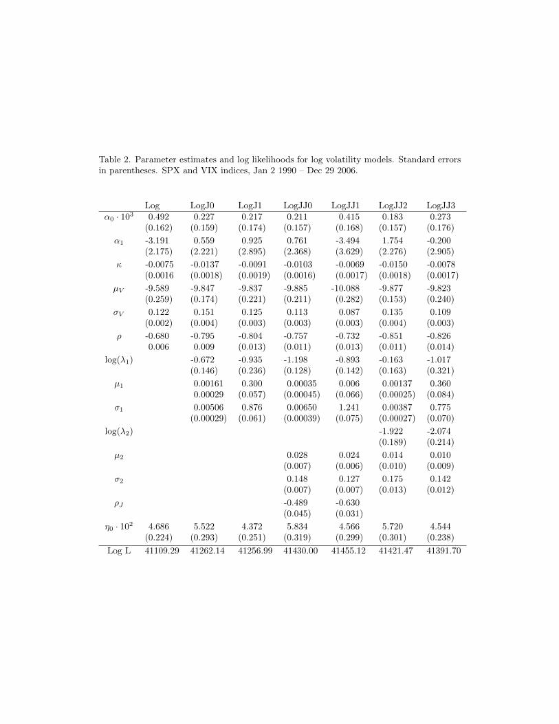
Parameter estimates and log likelihoods for the log volatility models are shown in

Table 2. All models are estimated fixing η∗1 = 0 and with no jump risk premium.

Alternative risk premium specifications are discussed in Section 4.3.

Including jumps in returns adds nearly 150 points to the log likelihood relative

to the model without jumps, consistent with previous findings that jumps provide

a big improvement in model fit (e.g., Bates 2000, Pan 2002). Whether jumps are

scaled by the volatility state (LogJ1) or not (LogJ0) makes little difference in log

likelihood. But in either case estimated jump distributions differ substantially from

what is typically found in the existing literature. We find that jumps occur nearly

every other day on average and have positive mean. This issue is discussed in more

detail in Section 4.2 below.

Including jumps in volatility (in addition to jumps in returns) provides an addi-

tional large gain in log likelihood, consistent with the findings of Eraker, Johannes,

and Polson (2003). The best of these models is LogJJ1, which uses scaled and cor-

related jumps. For this model the improvement in log likelihood is nearly 200 points

relative to the models with jumps in returns alone. Jumps occur about every other

day on average. The mean of return jumps does not differ significantly from zero

(see further discussion on this point in Section 4.2).

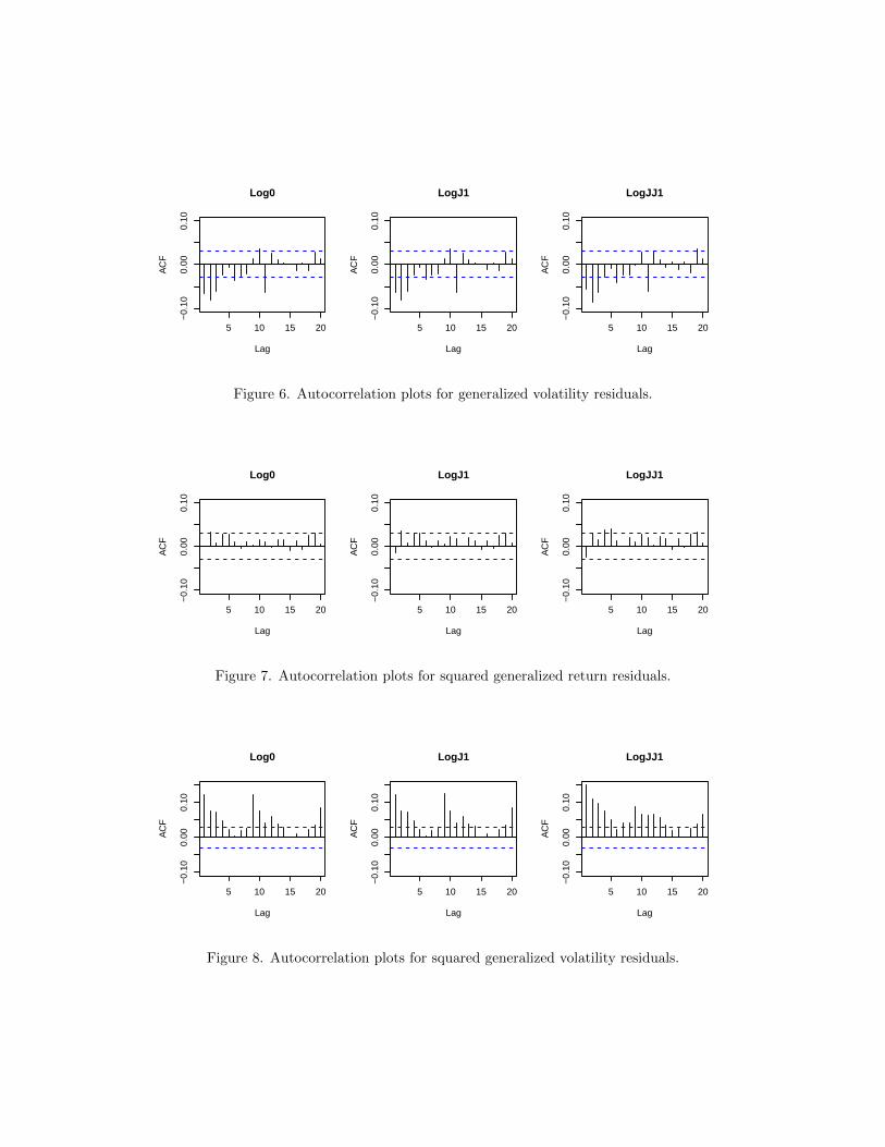
Figures 3-8 show diagnostic plots for the return and volatility generalized resid-

20

uals discussed in Section 3.3. The figures show results for the Log0, LogJ1 and

LogJJ1 models (no jumps, jumps in returns only and jumps in both returns and

volatility, respectively).

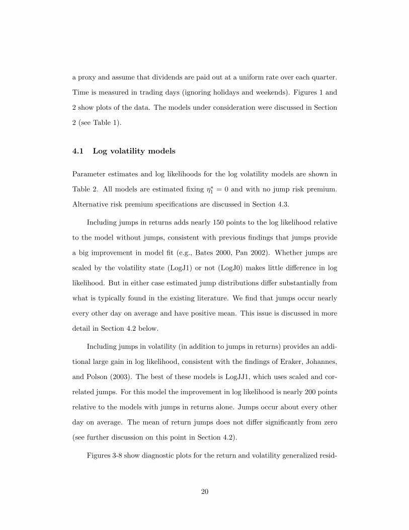
Figure 3 shows normal-quantile plots for the return residuals. Log0 shows the

expected problems in the left tail. The model is unable to account for days with

large negative returns. LogJ1 does a little better, but the problem still exists. The

issue is largely (but not entirely) resolved by LogJJ1.

Figure 4 shows normal-quantile plots for the volatility residuals. Again, Log0

and LogJ1, which do not include jumps in volatility, fail badly. The issue is most

severe in the right tail, but there are problems in the left tail as well. LogJJ1 does

much better, but some unexplained tail fatness remains, especially in the right tail.

Better results might be obtainable with more flexible distributions, e.g., addi-

tional jump processes. See also Durham (2007) for an alternative approach using

mixtures of normals.

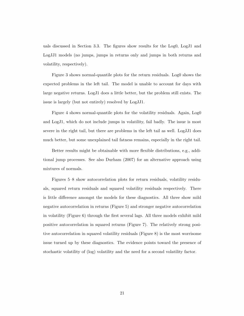
Figures 5–8 show autocorrelation plots for return residuals, volatility residu-

als, squared return residuals and squared volatility residuals respectively. There

is little difference amongst the models for these diagnostics. All three show mild

negative autocorrelation in returns (Figure 5) and stronger negative autocorrelation

in volatility (Figure 6) through the first several lags. All three models exhibit mild

positive autocorrelation in squared returns (Figure 7). The relatively strong posi-

tive autocorrelation in squared volatility residuals (Figure 8) is the most worrisome

issue turned up by these diagnostics. The evidence points toward the presence of

stochastic volatility of (log) volatility and the need for a second volatility factor.

21

4.2 Discussion of jump distributions

The estimated jump distributions found in this paper differ substantially from much

of the previous literature. While we find that jumps in returns are frequent (around

one every other day on average) and have near zero or even positive mean, the exist-

ing literature has typically found jumps in returns to occur relatively rarely and have

large, negative mean (e.g., Pan 2002). The form of the jump distributions typically

found in the previous literature is intuitively appealing given that it corresponds to

the “crash” days readily apparent in the data. So in this section we investigate the

plausibility of our findings. We defer a more detailed discussion of previous work

to Section 4.5, following the presentation of our results for affine models. However,

we note that Ferriani and Pastorello (2011), who use models and techniques similar

to those used in this paper, find return jump distributions that are consistent with

those reported here.

Figure 9 shows model innovations calculated as in (4) for LogJ1 and LogJJ1

with parameters reported in Table 2. Also shown are contours of the associated log

densities, calculated as in (5).

Visual inspection of this figure suggests that the estimated densities found by

the optimizer are reasonable, although more flexible models (e.g., multiple jump

components) could potentially provide somewhat better fits. The most severe prob-

lems that the models need to address are with respect to the volatility innovations,

so they expend most of their available degrees of freedom trying to fit that feature

of the data. These figures and the normal-quantile plots in the previous subsection

suggest that the models do about as well as might be hoped given the limited range

of flexibility available to them.

22

But some practitioners may feel strongly about the existence of infrequent re-

turn jumps with large negative mean. As an experiment, we tried refitting the

LogJ1 and LogJJ1 models with jump parameters fixed at various settings designed

to reflect such beliefs. In each case, all other model parameters were estimated

conditional on the fixed jump parameters.

For example, Figure 10 shows model innovations and density contours analogous

to Figure 9 but with jump parameters fixed at λ1 = 0.002, µ1 = −2.0, and σ1 =

2.0 (these parameter values are consistent with results from the extant literature

summarized in Table I of Broadie, Chernov, and Johannes (2007); experiments

with alternative parameter settings gave similar results). The results for LogJJ1

look reasonable. It does a little better at capturing the several observations in the

upper left corner of the figure. However, it does a little worse in other parts of

the distribution where there are far more observations. The log likelihood for the

constrained model is about 170 points worse than for the unconstrained model with

parameter values shown in Table 2. The results for LogJ1 are more interesting.

Including an extreme left-tail jump component in returns when there are no jumps

in volatility simply does not appear to be useful. While naive intuition may suggest

that such distributions could be plausible, they put significant probability mass

where there are few observations while failing to put additional mass in the region

where the targeted extreme observations are actually located.

Ultimately, we are interested in the shape of the predictive densities implied by

a particular model, not so much in the parameters themselves. None of these models

represent the true data generating process. We do not argue that our estimates of

the jump process are correct and the estimates found in previous work incorrect.

They are simply different ways of trying to fit misspecified models. Nonetheless,

23

optimizers are quite good at optimizing, and the maximum likelihood estimator

does have the attribute of minimizing Kullback-Leibler distance.

The practitioner with strong prior beliefs regarding the existence of infrequent

jumps with large negative mean can impose them on the model. But the loss in

model fit is substantial.

4.3 Discussion of risk premia

As described in Section 3.1, the risk-neutral model implies a mapping from latent

volatility states to corresponding values of IV, a model-free measure of volatility

based on observed option prices. Volatility dynamics implied by different risk-

neutral specifications or parameter values generate different mappings. The maxi-

mum likelihood estimator optimizes across candidate parameter vectors to find the

mapping for which the volatility states corresponding to observed IV provide the

best fit to observed returns (conditional on the parametric constraints imposed by

a particular model).

In this section we examine the implications of various assumptions for the diffu-

sive risk premia, η∗0 and η∗1, and a jump risk premium, η∗2. We assume the jump risk

premium is such that E[J∗1t2] = exp(Vt)(µ

21 + σ2

1 + η∗2) for the scaled jump models

and E[J∗1t2] = µ2

1 + σ21 + η∗2 for the unscaled models (note that the only place the

jump distribution under the risk-neutral measure enters the likelihood is through

the second moment of jump size in Equation (2)).

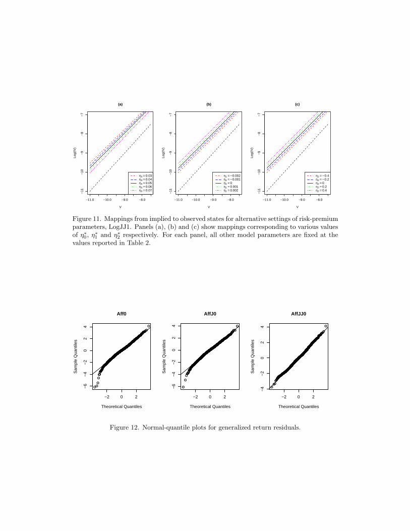
Figure 11 shows mappings from volatility state to IV for the LogJJ1 model

corresponding to several alternative values for η∗0 (left panel), η∗1 (center panel), and

η∗2 (right panel). In each panel, all other parameters are held fixed at the values

shown in Table 2.

24

There is little difference among the shapes of the mappings that result from

varying the different risk premium parameters. In each case, there is an upward

shift from volatility state to log IV, with the magnitude of this shift determined

by the size of the risk premium. But it makes little difference which of η∗0, η∗1 or

η∗2 is varied. All have essentially the same effect, making identification difficult.

If the model is fully optimized with any combination of these estimated as free

parameters, the log likelihood and other model parameters differ only minimally

from values reported in Table 2.

In the context of Pastorello, Patilea, and Renault (2003), η∗ = (η∗0, η∗1, η∗2) can

be thought of as a vector of nuisance parameters that determines (in conjunction

with the other model parameters) the mapping from observed to implied states.

This parameter vector is poorly identified. That is, different choices for η∗ can

generate essentially the same mapping. But this has no effect on identification of

the parameters of the physical model (which depends only on the mapping from

observed to implied states, not the particular value of η∗ used to construct it).

4.4 Affine models

Parameter estimates and log likelihoods for the affine models are shown in Table 3.

In contrast to the log volatility models, including a jump risk premium does improve

the performance of the affine models, so the results in Table 3 and elsewhere in

this section all include a jump risk premium. The form of the jump risk premium

is analogous to the one described in the context of the log volatility models (see

Section 4.3). We also estimate η∗1 but fix η∗0 = 0, following standard practice (e.g.,

Bates (2000); see also discussion of alternative risk premium specifications below).

Although we do include a jump risk parameter in the model, our estimates of

25

it may not have much practical value. As noted by Broadie, Chernov, and Johannes

(2007), more information (e.g., from either the term structure of implied volatility

or shape of the implied volatility smile across moneyness) is needed to disentangle

the effects of the various sources of risk premium in any meaningful way. This paper

makes no use of such information, nor does it intend to have explanatory power for

these features of the data.

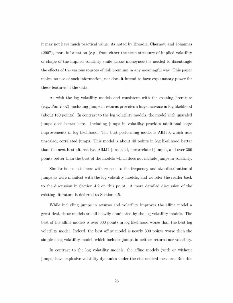
As with the log volatility models and consistent with the existing literature

(e.g., Pan 2002), including jumps in returns provides a huge increase in log likelihood

(about 160 points). In contrast to the log volatility models, the model with unscaled

jumps does better here. Including jumps in volatility provides additional large

improvements in log likelihood. The best performing model is AffJJ0, which uses

unscaled, correlated jumps. This model is about 40 points in log likelihood better

than the next best alternative, AffJJ2 (unscaled, uncorrelated jumps), and over 300

points better than the best of the models which does not include jumps in volatility.

Similar issues exist here with respect to the frequency and size distribution of

jumps as were manifest with the log volatility models, and we refer the reader back

to the discussion in Section 4.2 on this point. A more detailed discussion of the

existing literature is deferred to Section 4.5.

While including jumps in returns and volatility improves the affine model a

great deal, these models are all heavily dominated by the log volatility models. The

best of the affine models is over 600 points in log likelihood worse than the best log

volatility model. Indeed, the best affine model is nearly 300 points worse than the

simplest log volatility model, which includes jumps in neither returns nor volatility.

In contrast to the log volatility models, the affine models (with or without

jumps) have explosive volatility dynamics under the risk-neutral measure. But this

26

is more likely an artifact of model misspecification than a meaningful feature of the

data. Models with explosive volatility dynamics are essentially useless for forecasting

volatility at any time horizon other than the specific horizon at which the model

is estimated (corresponding to the one-month horizon of the VIX index in this

application).

Figures 12 - 17 show diagnostic plots for several of the affine models. These

diagnostics are largely similar to those for the log volatility models shown in Section

4.1, but there are some important differences. Figure 12, which shows normal-

quantile plots for generalized return residuals, suggests that AffJJ0 actually does a

little better than the best of the log volatility models in fitting the marginal return

distribution. However, the normal-quantile plots for the generalized volatility resid-

uals (Figure 13) are more problematic. Including jumps in volatility (AffJJ0) helps

a great deal, as expected, and this model matches the right tail of the distribution

quite well. But, there are serious problems in the left tail. Given that the exponen-

tial distribution, which is used to describe volatility jumps in this model, generates

a long tail in one direction (depending on the sign of the coefficient) but nothing in

the other, this result should not be a complete surprise.

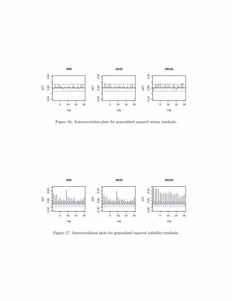
The autocorrelation plots shown in Figures 14 - 17 are mostly similar to those

for the log models (Section 4.1). However, the autocorrelation plots for squared

volatility residuals (Figure 17) are noticeably worse than those for the log volatility

models (Figure 8). The affine models are poorly specified for volatility of volatility,

as pointed out by e.g. Poteshman (1998) and Jones (2003).

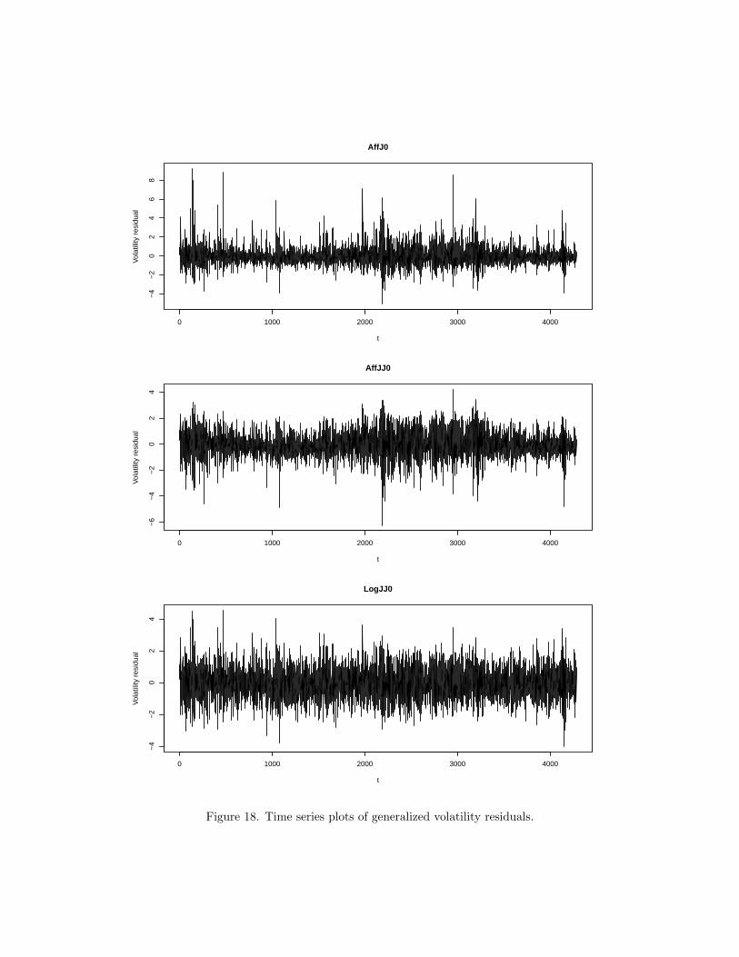
Figure 18 shows time-series plots of the generalized volatility residuals for AffJ0

and AffJJ0. The autocorrelation pattern is clearly evident in both, although in

AffJ0 it is to some extent masked by the extreme outliers (recall that under the

27

hypothesis that the model is the true data generating process, these should be iid

standard normal). In either case, the generalized residuals tend to be too small

(in absolute value) when the observed IV is low and too large when the observed

IV is high. It makes little difference whether we use scaled or unscaled, correlated

or uncorrelated jumps: the resulting figures are nearly identical in all cases. For

reference, an analogous plot is shown for LogJJ0. There is still some autocorrelation

in the generalized residuals here, but the problem is much less severe. The square-

root specification for volatility of volatility simply does not fit the data. Jumps in

volatility help but do not resolve the problem.

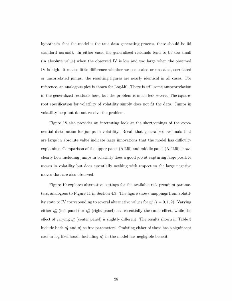
Figure 18 also provides an interesting look at the shortcomings of the expo-

nential distribution for jumps in volatility. Recall that generalized residuals that

are large in absolute value indicate large innovations that the model has difficulty

explaining. Comparison of the upper panel (AffJ0) and middle panel (AffJJ0) shows

clearly how including jumps in volatility does a good job at capturing large positive

moves in volatility but does essentially nothing with respect to the large negative

moves that are also observed.

Figure 19 explores alternative settings for the available risk premium parame-

ters, analogous to Figure 11 in Section 4.3. The figure shows mappings from volatil-

ity state to IV corresponding to several alternative values for η∗i (i = 0, 1, 2). Varying

either η∗0 (left panel) or η∗2 (right panel) has essentially the same effect, while the

effect of varying η∗1 (center panel) is slightly different. The results shown in Table 3

include both η∗1 and η∗2 as free parameters. Omitting either of these has a significant

cost in log likelihood. Including η∗0 in the model has negligible benefit.

28

4.5 Discussion of previous work

This section provides a brief discussion of some findings of prior work regarding

jumps and return distributions.

A number of papers, including Chernov, Gallant, Ghysels, and Tauchen (2003)

and Durham (2007), have estimated models based on returns alone and found ev-

idence of long left tails in the return distributions. But, such studies do not make

use of the more informative signal about the volatility state that is available using

option prices. As noted by Andersen, Bollerslev, Diebold, and Ebens (2001) in the

context of high-frequency estimates of the volatility state, if returns are normal-

ized by more informative estimates of volatility, much of this non-Gaussianity may

disappear.

Bates (2000) looks at affine models with one or two volatility factors and jumps

in returns only. While he finds evidence of infrequent jumps with large negative

mean, his findings pertain to risk-neutral rather than physical models.

Pan (2002) looks at affine models which include jumps in returns but not volatil-

ity. Under her preferred SVJ0 model, she finds evidence of jumps that are relatively

rare with small but negative mean and high dispersion under the physical model.

But these findings are difficult to compare to those of this paper: she looks at weekly

data, which have limited explanatory power regarding the distribution of daily re-

turns; her sample is small (only 8 years of weekly data, about 400 observations); and

she uses a simulated method of moments estimator (which can give very different

results from likelihood-based estimators in the presence of model misspecification).

Although Pan reports that her model is not rejected by the joint time-series of re-

turns and implied volatility states, the results reported in Section 4.4 of this paper

29

suggest that this may be because her sample size is small and her tests lack power.

Eraker, Johannes, and Polson (2003) look at affine models with jumps in volatil-

ity and returns, including models that are essentially identical to the AffJJ0 and

AffJJ2 models examined in this paper. They use (likelihood-based) Bayesian meth-

ods and find evidence of infrequent return jumps with large negative mean in the

physical model. But they rely on returns data alone to extract volatility states. As

noted above, this results in a substantially less informative signal about volatility

than using option prices. Furthermore, they limit the maximum number of jumps

per day to one, which may bias the results in favor of low jump intensity. And

finally, their findings may be dictated by the priors they use. They use priors that

“are always consistent with the intuition that jumps are ‘large’ and infrequent.” The

prior places “low probability on the jump sizes being small” and “low probability

on the daily jump probability being greater than 10 percent.”

Eraker (2004) looks at affine models with jumps in returns and volatility. Using

observed option prices to back out volatility states, Eraker also finds evidence of

infrequent jumps with large negative mean. But, as with Eraker, Johannes, and

Polson (2003), the maximum number of jumps per day is limited to one. Although

Eraker uses Bayesian estimation, his priors are not reported. If they are consistent

with Eraker, Johannes, and Polson (2003), however, his results could be biased as

noted above. Also, Eraker’s sample is relatively small, consisting only of data from

Jan 1 1987 through Dec 31 1990 (about 1000 observations). As noted by Eraker,

this sample period may not be representative.

Broadie, Chernov, and Johannes (2007) look at affine models that include jumps

in returns and volatility, but they rely on estimates for the physical model from

Eraker, Johannes, and Polson (2003).

30

In contrast to the work summarized above, Ferriani and Pastorello (2011) look

at log models similar to some of those used in this paper (but with jumps in returns

only), use a large sample of daily data (Jan 4, 1996 – Dec 30, 2005), and apply

techniques closely related to those used in this paper. In their Log-Ja model (which

corresponds to the LogJ0 model in this paper), they find that under the physical

measure jumps occur frequently, have low dispersion, and have mean near zero.

Their findings in this regard are consistent with those of this paper.

5 Conclusions

This paper demonstrates techniques for joint analysis of physical and risk-neutral

models for financial assets. In contrast to much of the existing literature which fo-

cuses on affine models for reasons of computational tractability, these techniques are

applicable to a broad class of diffusion models, including log volatility models with

jumps in both returns and volatility. We demonstrate efficient techniques for invert-

ing the risk-neutral measure in order to get implied volatility states from observed

panels of option prices, maximum likelihood estimation, and a highly informative

set of diagnostics.

The application looks at SPX and VIX index data. Consistent with previous

work, including jumps in returns provides a large increase in log likelihood relative to

models with no jumps, and including jumps in volatility provides an additional large

increase. In contrast to previous work, we find that return jumps occur frequently,

are mostly small, and have near zero mean.

Log volatility models are dramatically better than the corresponding affine mod-

els. Including jumps, whether in returns alone or together with jumps in volatility,

31

does not change this result. The best log volatility model is over 600 points in log

likelihood better than any of the affine models. The best of the affine models is

nearly 300 points worse than even the simple log volatility model with no jumps.

The affine models also exhibit severe problems with the diagnostics. For exam-

ple, all of the affine models exhibit substantial autocorrelation in squared volatility

generalized residuals. The square root specification for volatility of volatility simply

does not fit the data; including jumps is of little help here. Also, while affine models

with exponential jumps in volatility are able to match the right tail of volatility

innovations, they are not able to match the left tail. Exponential jumps are either

always positive or always negative, depending on the sign of the coefficient. The

fitted models can generate large upward moves in volatility, but not large downward

moves, such as are also exhibited by the data.

The availability of powerful diagnostics based on generalized residuals is a useful

tool for model exploration. Although it is easy to perform conventional tests (e.g.,

Jarque-Bera or Box-Pierce) using the generalized residuals, we do not report these

in the paper. All the models are rejected at far beyond conventional significance

levels on at least one test. One would have to be almost hopelessly optimistic to

believe that any of the models examined in this paper was the true data generating

process. Failure to reject a model in exercises such as this should more likely be

interpreted as a sign of insufficient sample size or tests with low power rather than an

indication that one has found the true data generating process. Powerful diagnostics

are a good thing; failure to find evidence of defective models is a serious liability.

32

References

Andersen, T., T. Bollerslev, F. Diebold, and H. Ebens (2001): “The distributionof realized stock return volatility,” Journal of Financial Economics, 61, 43–76.

Andersen, T., T. Bollerslev, F. Diebold, and P. Labys (2003): “Modeling andforecasting realized volatility,” Econometrica, 71(2), 579–625.

Andersen, T. G., L. Benzoni, and J. Lund (2002): “An Empirical Investigation ofContinuous-Time Equity Return Models,” Journal of Finance, 57, 1239–1284.

Barndorff-Nielsen, O. E., and N. Shephard (2002): “Econometric Analysis of Real-ized Volatility and Its Use in Estimating Stochastic Volatility Models,” Journal of theRoyal Statistical Society, Series B, 64, 253–280.

Bates, D. S. (2000): “Post-’87 Crash Fears in the S&P 500 Futures Option Market,”Journal of Econometrics, 94, 181–238.

(2006): “Maximum Likelihood Estimation of Latent Affine Processes,” Review ofFinancial Studies, 19(3), 909–965.

Bollerslev, T., and H. Zhou (2006): “Volatility puzzles: a simple framework for gaugingreturn-volatility regressions,” Journal of Econometrics, 131, 123–150.

Britten-Jones, M., and A. Neuberger (2000): “Option prices, implied price processes,and stochastic volatility,” Journal of Finance, 55, 839–866.

Broadie, M., M. Chernov, and M. Johannes (2007): “Model specification and riskpremia: evidence from futures options,” Journal of Finance, 62(3), 1453–1490.

Chernov, M., A. R. Gallant, E. Ghysels, and G. Tauchen (2003): “AlternativeModels for Stock Price Dynamics,” Journal of Econometrics, 116, 225–257.

Chernov, M., and E. Ghysels (2000): “A Study Towards a Unified Approach to theJoint Estimation of Objective and Risk Neutral Measures for the Purposes of OptionsValuation,” Journal of Financial Economics, 56, 407–458.

Christensen, B., and N. Prabhala (1998): “The realtion between implied and realizedvolatility,” Journal of Financial Economics, 50, 125–150.

Christoffersen, P., K. Jacobs, and K. Mimouni (2006): “Models for S&P 500 dynam-ics: Evidence from realized volatility, daily returns, and option prices,” Unpublishedmanuscript, McGill University.

Corrado, C., and T. Miller (2005): “The forecast quality of CBOE implied volatilityindexes,” Journal of Futures Markets, 25(4), 339–373.

Duffie, D., J. Pan, and K. J. Singleton (2000): “Transform analysis and asset pricingfor affine jump-diffusions,” Econometrica, 68, 1343–1376.

Durbin, J., and S. Koopman (1997): “Monte Carlo Maximum Likelihood Estimation forNon-Gaussian State Space Models,” Biometrika, 84(3), 669–684.

33

Durham, G. B. (2006): “Monte Carlo Methods for Estimating, Smoothing, and FilteringOne- and Two-Factor Stochastic Volatility Models,” Journal of Econometrics, 133(1),273–305.

(2007): “SV Mixture Models with Application to S&P 500 Index Returns,” Journalof Financial Economics, 85(3), 822–856.

Durham, G. B., and A. R. Gallant (2002): “Numerical Techniques for Simulated Max-imum Likelihood Estimation of Stochastic Differential Equations,” Journal of Businessand Economic Statistics, 20(3), 297–316.

Elerian, O., S. Chib, and N. Shephard (2001): “Likelihood Inference for DiscretelyObserved Non-linear Diffusions,” Econometrica, 69, 959–993.

Eraker, B. (2001): “MCMC Analysis of Diffusion Models with Application to Finance,”Journal of Business and Economic Statistics, 19(2), 177–191.

Eraker, B. (2004): “Do Stock Prices and Volatility Jump? Reconciling Evidence fromSpot and Option Prices,” Journal of Finance, 59, 1367–1403.

Eraker, B., M. Johannes, and N. G. Polson (2003): “The Impact of Jumps in Volatil-ity and Returns,” Journal of Finance, 58, 1269–1300.

Ferriani, F., and S. Pastorello (2011): “Estimating and testing non-affine optionpricing models with a large unbalanced panel of options,” Unpublished manuscript.

Fleming, J., B. Ostdiek, and R. Whaley (1995): “Predicting stock market volatility:A new measure,” Journal of Futures Markets, 15(3), 265–302.

Fouque, J.-P., G. Papanicolaou, and K. Sircar (2000): Derivatives in financial mar-kets with stochastic volatility. Cambridge University Press, Cambridge, UK.

Gallant, A. R., and G. E. Tauchen (1996): “Which Moments to Match?,” EconometricTheory, 12, 657–681.

Garcia, R., M.-A. Lewis, S. Pastorello, and E. Renault (2011): “Estimation ofobjective and risk-neutral distributions based on moments of integrated volatility,”Journal of Econometrics, 160, 22–32.

Ghysels, E., P. Santa-Clara, and R. Valkanov (2006): “Predicting volatility: Get-ting the most out of return data sampled at different frequencies,” Journal of Econo-metrics, 131(1-2), 59–95.

Jacquier, E., N. G. Polson, and P. E. Rossi (1994): “Bayesian Analysis of StochasticVolatility Models,” Journal of Business and Economic Statistics, 12(4), 371–389.

(2004): “Bayesian Analysis of Stochastic Volatility Models with Fat-Tails andCorrelated Errors,” Journal of Econometrics, 122(1), 185–212.

Jiang, G., and Y. Tian (2005): “The model-free implied volatility and its informationcontent,” Review of Financial Studies, 18(4), 1305–1342.

34

Jones, C. S. (2003): “The Dynamics of Stochastic Volatility: Evidence from Underlyingand Options Markets,” Journal of Econometrics, 116, 181–224.

Kim, S., N. Shephard, and S. Chib (1998): “Stochastic Volatility: Likelihood Inferenceand Comparison with ARCH Models,” Review of Economic Studies, 65, 361–393.

Kloeden, P., and E. Platen (1992): Numerical Solution of Stochastic Differential Equa-tions. Springer Verlag, Berlin.

Lewis, A. (2000): Option valuation under stochastic volatility. Finance Press, NewportBeach, CA.

Liesenfeld, R., and J.-F. Richard (2003): “Univariate and Multivariate StochasticVolatility Models: Estimation and Diagnostics,” Journal of Empirical Finance, 10,505–531.

Pan, J. (2002): “The Jump-Risk Premia Implicit in Options: Evidence From an IntegratedTime-Series Study,” Journal of Financial Economics, 63, 3–50.

Pastorello, S., V. Patilea, and E. Renault (2003): “Iterative and recursive estima-tion in structural nonadaptive models,” Journal of Business and Economic Statistics,21(4), 449–482.

Pastorello, S., E. Renault, and N. Touzi (2000): “Statistical inference for random-variance option pricing,” Journal of Business and Economic Statistics, 18(3), 358–367.

Pedersen, A. R. (1995): “A New Approach to Maximum Likelihood Estimation forStochastic Differential Equations Based on Discrete Observations,” Scandinavian Jour-nal of Statistics, 22, 55–71.

Poteshman, A. M. (1998): “Estimating a general stochastic variance model from optionprices,” Unpublished manuscript.

Romano, M., and N. Touzi (1997): “Contingent claims and market completeness in astochastic volatility model,” Mathematical Finance, 7(399-412).

Shephard, N., and M. Pitt (1997): “Likelihood analysis of Non-Gaussian measurementTime Series,” Biometrika, 84(3), 653–667.

35

Table 1. Model specifications.

Log

PhysicaldYt = (rt − qt + α0 + (α1 − 0.5) exp(Vt)− λ1µ1t) dt+ exp(Vt/2) dW1t + J1t dN1t

dVt = (κ(Vt − µV )− λ2µ2t) dt+ σV dW2t + J2t dN2t

Risk-neutraldYt = (rt − qt − 0.5 exp(Vt)− λ1µ1t) dt+ exp(Vt/2) dW ∗

1t + J∗1t dN1t

dVt = (κ(Vt − µV ) + η∗1Vt + η∗0 − λ2µ2t) dt+ σV dW∗2t + J∗

2t dN2t

Affine

PhysicaldYt = (rt − qt + α0 + (α1 − 0.5)Vt − λ1µ1t) dt+

√Vt dW1t + J1t dN1t

dVt = (κ(Vt − µV )− λ2µ2t) dt+ σV√Vt dW2ty + J2t dN2t

Risk-neutraldYt = (rt − qt − 0.5Vt − λ1µ1t) dt+

√Vt dW

∗1t + J∗

1t dN1t

dVt = (κ(Vt − µV ) + η∗1Vt + η∗0 − λ2µ2t) dt+ σV√Vt dW

∗2t + J∗

2t dN2t

Table 2. Parameter estimates and log likelihoods for log volatility models. Standard errorsin parentheses. SPX and VIX indices, Jan 2 1990 – Dec 29 2006.

Log LogJ0 LogJ1 LogJJ0 LogJJ1 LogJJ2 LogJJ3α0 · 103 0.492 0.227 0.217 0.211 0.415 0.183 0.273

(0.162) (0.159) (0.174) (0.157) (0.168) (0.157) (0.176)

α1 -3.191 0.559 0.925 0.761 -3.494 1.754 -0.200(2.175) (2.221) (2.895) (2.368) (3.629) (2.276) (2.905)

κ -0.0075 -0.0137 -0.0091 -0.0103 -0.0069 -0.0150 -0.0078(0.0016 (0.0018) (0.0019) (0.0016) (0.0017) (0.0018) (0.0017)

µV -9.589 -9.847 -9.837 -9.885 -10.088 -9.877 -9.823(0.259) (0.174) (0.221) (0.211) (0.282) (0.153) (0.240)

σV 0.122 0.151 0.125 0.113 0.087 0.135 0.109(0.002) (0.004) (0.003) (0.003) (0.003) (0.004) (0.003)

ρ -0.680 -0.795 -0.804 -0.757 -0.732 -0.851 -0.8260.006 0.009 (0.013) (0.011) (0.013) (0.011) (0.014)

log(λ1) -0.672 -0.935 -1.198 -0.893 -0.163 -1.017(0.146) (0.236) (0.128) (0.142) (0.163) (0.321)

µ1 0.00161 0.300 0.00035 0.006 0.00137 0.3600.00029 (0.057) (0.00045) (0.066) (0.00025) (0.084)

σ1 0.00506 0.876 0.00650 1.241 0.00387 0.775(0.00029) (0.061) (0.00039) (0.075) (0.00027) (0.070)

log(λ2) -1.922 -2.074(0.189) (0.214)

µ2 0.028 0.024 0.014 0.010(0.007) (0.006) (0.010) (0.009)

σ2 0.148 0.127 0.175 0.142(0.007) (0.007) (0.013) (0.012)

ρJ -0.489 -0.630(0.045) (0.031)

η0 · 102 4.686 5.522 4.372 5.834 4.566 5.720 4.544(0.224) (0.293) (0.251) (0.319) (0.299) (0.301) (0.238)

Log L 41109.29 41262.14 41256.99 41430.00 41455.12 41421.47 41391.70

Table 3. Parameter estimates and log likelihoods for affine models. Standard errors inparentheses. SPX and VIX indices, Jan 2 1990 – Dec 29 2006.

Aff AffJ0 AffJ1 AffJJ0 AffJJ1 AffJJ2 AffJJ3α0 · 103 -0.011 0.322 -0.004 -0.603 -0.151 0.282 -0.002

(0.120) (0.184) (0.194) (0.198) (0.179) (0.173) (0.180)

α1 3.023 -0.495 4.242 10.554 6.456 0.008 4.286(2.256) (2.733) (3.012) (2.977) (2.907) (2.728) (3.025)

κ -0.016 -0.012 -0.012 -0.038 -0.034 -0.023 -0.024(0.002) (0.003) (0.003) (0.003) (0.003) (0.003) (0.003)

µV · 103 0.097 0.077 0.082 0.084 0.086 0.077 0.081(0.011) (0.017) (0.016) (0.006) (0.006) (0.008) (0.008)

σV · 103 1.380 1.371 1.324 1.023 1.059 1.218 1.142(0.024) (0.027) (0.029) (0.028) (0.028) (0.031) (0.031)

ρ -0.658 -0.771 -0.786 -0.663 -0.671 -0.781 -0.768(0.007) (0.010) (0.012) (0.010) (0.010) (0.010) (0.013)

log(λ1) -0.321 -1.115 -2.490 -2.860 -0.198 -1.367(0.137) (0.223) (0.116) (0.133) (0.167) (0.264)

µ1 0.0014 0.341 0.0016 -0.019 0.0008 0.230(0.0002) (0.063) (0.0014) (0.208) (0.0002) (0.073)

σ1 0.0044 0.921 0.0087 1.288 0.0042 1.023(0.0002) (0.070) (0.0008) (0.104) (0.0003) (0.087)

log(λ2) -3.355 -3.408(0.191) (0.190)

µ2 · 105 2.267 2.673 2.365 2.477(0.203 (0.292 (0.341) (0.355)

ρJ -0.0096 -0.739(0.0015) (0.200)

η1 · 102 4.869 5.608 -11.030 8.338 24.915 6.669 10.655(0.237) (0.336) (12.988) (0.413) (3.794) (0.362) (3.747)

η2 · 105 0.006 -0.521 -0.007(0.005) (0.086) (0.005)

η2 10.199 -18.369 -2.503(12.294) (2.391) (1.290)

Log L 40338.47 40498.16 40473.57 40812.64 40769.81 40772.86 40728.71

1990 1995 2000 2005

6.0

6.5

7.0

Log SPX

Time

Log

SP

X

1990 1995 2000 2005

−0.

06−

0.02

0.02

0.04

0.06

SPX log returns

Time

SP

X lo

g re

turn

s

1990 1995 2000 2005

1020

3040

VIX

Time

VIX

Figure 1. Time-series plots of the log SPX, SPX log returns, and VIX index, Jan 2 1990 –Dec 29 2006.

1990 1995 2000 2005

24

68

3−month T−bill rate

Time

Rat

e

1990 1995 2000 2005

1.5

2.5

3.5

SP 500 dividend rate

Time

Rat

e

Figure 2. Time-series plots of the three-month Treasury bill rate and S&P 500 dividendpayout rate, Jan 2 1990 – Dec 29 2006.

●

●●

●

●

●

●

●

●

●

●

●●

●

●

●

●

●●●

●

●

●●

●

●

●●

●

●●

●

●

●

●●●

●

●●●

●

●

●

●

●

●

●

●

●●

●

●

●●

●

●●

●

●●●●

●

●

●●

●●●

●

●●

●●●

●

●

●●

●

●●●

●

●●

●●●

●

●

●●●●

●

●●

●

●

●

●●●

●

●●●

●

●

●

●●

●

●

●●

●

●

●

●

●●

●●

●

●

●

●

●

●●

●●

●

●

●

●

●

●●

●●

●●

●

●

●●

●

●●

●

●

●●

●

●

●

●●

●

●

●

●

●

●

●

●●

●

●

●●

●

●●

●●

●

●

●

●

●

●●

●

●

●

●

●

●

●

●

●●

●●

●

●

●●

●

●

●

●

●

●

●●

●●

●

●

●

●

●●

●

●

●

●

●

●

●●

●●●

●

●

●●●

●●

●

●

●

●●

●

●

●●●

●

●

●

●●

●●

●

●

●

●

●●

●

●●

●

●

●●

●

●

●●●

●●

●

●

●

●

●

●

●

●

●

●

●

●

●

●●

●

●

●

●

●

●

●●●●

●

●

●●

●

●

●

●

●●

●

●●

●

●

●●

●

●

●

●

●●

●

●

●

●

●●

●●

●

●

●

●

●

●●●

●

●

●

●

●

●

●

●

●●

●

●

●

●

●

●

●●

●●

●●

●

●

●

●

●

●

●●

●

●

●

●

●●

●

●

●

●

●

●

●

●●

●

●●

●●

●

●●

●

●

●

●

●●

●

●●

●

●

●●

●

●●

●●

●

●

●

●

●

●

●●

●

●●

●

●●

●●

●

●●

●

●

●

●●●

●

●

●●●

●●

●

●●

●

●

●

●

●

●●

●

●●

●●

●

●

●

●

●●

●●●●

●

●

●●

●

●●

●

●

●

●

●

●

●

●

●●

●

●●●

●

●●●

●●

●

●

●●

●

●

●

●

●

●

●●

●

●●

●●

●●

●

●

●

●

●●

●

●

●●●

●

●

●

●

●

●●

●

●

●

●

●

●

●

●

●

●

●

●

●

●●●●

●●

●

●●

●

●

●●

●

●●

●

●●●

●

●

●●●

●

●

●

●

●

●

●●

●

●

●

●

●●

●

●

●●

●●

●

●

●●●

●

●

●

●

●●

●●

●

●

●

●

●

●

●

●

●

●

●

●●

●●

●●●

●

●

●

●

●●

●●●

●

●

●

●

●

●

●

●

●●

●

●●

●●

●

●

●

●●

●●

●

●●

●

●●●

●●●

●

●●●

●

●

●●

●●

●●

●

●●

●●

●

●

●

●

●

●

●●

●

●

●

●●

●

●

●●

●

●

●

●

●

●

●

●

●●●

●●

●●●●

●

●●

●

●

●

●●

●

●

●●

●

●●

●●

●

●

●

●

●●

●●

●●●

●●

●

●●●●●

●

●

●

●●●

●

●●

●

●

●●

●

●

●

●

●

●●

●

●

●●

●

●

●

●

●

●●

●

●

●

●

●●●

●●

●

●

●●

●●

●

●

●●

●

●

●

●●

●

●

●

●●

●●

●

●

●●●

●

●

●

●

●

●●

●

●

●

●

●

●

●

●●●

●●

●

●

●●

●

●●●

●●

●

●●

●●

●

●

●●●

●

●

●

●●

●

●●

●

●●

●●●

●●

●●

●

●●

●

●

●

●

●

●

●

●●

●

●

●

●

●

●

●

●

●

●

●

●●

●

●

●●

●●

●

●

●

●●●●

●

●

●

●

●●

●

●

●●

●

●

●●

●

●●

●

●

●

●

●

●

●

●

●

●

●

●

●

●

●●

●

●

●●●

●

●●●●

●●●●

●

●

●●

●●

●

●●●

●

●●

●

●●

●●●

●

●

●

●

●

●●●

●

●●●

●●●

●●●●

●

●

●

●

●

●

●

●

●●

●

●

●

●●

●●

●

●●

●

●

●

●●

●

●

●

●●

●●

●

●

●

●

●

●

●

●

●

●

●

●

●

●

●●

●

●

●●

●

●

●

●●

●

●

●

●●

●

●

●

●●

●

●●

●

●

●●

●●

●

●●

●

●

●

●

●

●

●

●●

●●

●

●●

●

●

●

●

●

●●

●●

●

●

●

●

●

●

●●

●●●

●●

●●●●

●

●●

●

●●●

●●●

●

●

●

●●

●

●

●

●

●

●

●

●

●

●●

●●

●●

●

●

●●

●●

●●

●

●●

●

●●

●

●

●

●

●●

●

●

●

●

●

●

●

●

●

●

●

●

●

●●

●

●●

●

●

●

●

●

●●

●

●

●

●

●

●●

●●●

●

●●

●

●●

●●

●

●

●●

●●

●

●●

●

●●

●

●

●

●

●

●

●

●●

●●

●

●

●●

●●●

●

●

●●●

●

●

●

●●●

●

●●

●

●

●

●

●●

●

●●

●

●

●

●

●

●

●●●

●●●

●●

●●

●●

●●

●●

●

●

●

●

●

●

●

●●

●

●●

●●

●

●

●

●●●

●

●

●●

●●

●

●●

●

●

●

●

●

●●

●

●●

●

●

●

●●●

●

●

●●●●

●

●●

●

●●●

●●

●●●●

●●

●

●●

●

●●

●●

●

●

●

●

●

●●

●●

●

●

●

●●

●

●

●●

●

●

●

●●

●

●

●●

●

●

●

●

●

●

●●

●

●

●

●

●

●

●●

●

●

●

●

●

●●

●

●

●●

●●

●●●

●●

●●

●

●

●

●●

●

●

●

●

●

●

●●●●

●

●●

●●

●●

●

●●

●●

●

●●●●

●

●●

●●

●●

●

●

●●

●

●

●

●

●

●●

●

●●

●●

●

●

●

●

●●

●

●

●●

●

●●●

●

●

●

●●

●

●

●

●

●

●

●

●

●●

●

●

●

●

●

●

●

●

●●

●●

●

●

●

●

●

●

●●

●

●●

●

●

●●

●

●

●

●

●●

●●

●

●

●●●

●

●

●

●

●●●

●

●

●

●

●

●●●

●●

●

●

●

●

●

●

●●●

●

●●●●

●

●

●

●

●

●

●●●

●

●

●

●

●●

●

●

●●●●

●

●●●●●

●

●●●

●

●

●

●

●

●●

●●

●

●

●

●

●●

●

●●

●●

●

●●●●●●●

●

●●

●●

●

●

●●

●

●●

●

●

●●

●

●

●

●

●

●

●●●

●

●●

●

●●

●●

●

●●

●●

●

●

●●

●●

●●

●

●●

●

●

●●

●●

●

●●

●

●●

●

●

●●

●●

●●●●●●●

●

●

●

●

●●●

●

●

●

●●●

●●

●

●

●●

●

●

●

●

●

●●

●●●

●

●

●

●●

●

●

●

●●

●●●

●

●

●●

●

●

●

●

●

●

●

●●

●

●

●

●●

●

●

●

●

●

●

●

●

●●

●

●

●

●●

●

●●

●●

●

●

●

●

●●

●

●

●

●

●

●

●

●

●

●

●

●

●

●

●●

●

●

●

●

●

●●

●

●

●

●●

●●●

●

●

●●

●●

●

●

●

●●●

●●

●

●

●●

●

●

●

●

●●●

●

●

●

●

●

●

●

●

●●

●

●

●●

●

●

●

●●

●

●

●●

●

●●

●

●

●

●●

●

●●

●●

●

●

●

●

●

●●

●

●

●

●●

●

●

●

●●●

●●

●

●

●

●

●●

●●

●●

●

●

●●

●

●

●

●

●

●

●

●

●●●

●

●●●

●

●

●

●

●●

●●●

●

●

●

●

●

●

●●●

●●●

●●

●

●●●

●●

●

●●●●

●

●●

●

●

●

●

●

●

●

●

●

●

●

●●●

●●

●

●

●●●

●

●

●

●

●

●●

●

●

●

●

●

●●●

●

●

●●

●

●●

●

●

●

●

●●

●●

●

●

●●

●

●●●

●

●

●

●●●

●

●●●

●

●

●●

●

●

●

●

●●

●

●

●

●

●●

●

●

●

●●

●

●

●

●

●

●

●●

●

●

●●●

●

●

●

●●

●●

●●●

●●

●●

●

●

●●

●

●

●●●

●●

●

●

●

●

●

●

●●●

●

●

●

●●

●

●

●

●

●●

●

●

●

●

●●

●

●

●

●●

●

●

●

●

●

●

●●

●

●●

●

●●

●

●

●

●

●

●

●

●●

●

●

●

●

●

●

●

●

●●

●

●

●

●

●

●

●●●

●●

●

●●

●●

●●●

●●

●

●

●

●

●

●●●

●

●●

●●

●●

●

●●●

●

●

●●●

●●

●

●●

●●

●●

●

●

●

●●●

●●

●

●●

●

●●●

●

●●

●

●

●●

●

●●●●

●●

●

●

●●

●

●

●

●

●

●

●

●

●

●

●

●

●

●

●●

●

●

●●

●

●

●●

●

●

●

●

●

●

●

●

●

●●

●

●

●●

●

●●

●●

●

●

●

●

●

●

●

●

●

●

●

●

●

●

●

●●●

●

●

●

●

●

●

●●

●

●

●●

●

●

●

●

●

●

●

●

●●

●

●

●

●

●

●●

●

●

●●

●

●

●●

●●●

●●●

●

●

●

●

●

●

●●

●

●

●●

●

●●

●●

●

●

●

●●

●

●

●

●

●

●●

●●

●

●●

●

●

●

●

●

●●●

●●

●

●

●

●

●●

●●●

●

●

●

●

●●

●

●

●

●

●●

●

●

●

●

●

●

●

●

●

●

●●

●

●

●

●

●●

●

●

●

●

●

●●

●●

●●

●

●

●

●

●

●

●

●●

●

●

●

●

●

●

●

●

●

●

●●

●

●

●●

●

●

●

●●

●

●

●

●●

●●●●

●

●●●

●

●

●

●

●●

●

●

●

●

●

●●

●

●●

●

●●

●

●

●●●

●

●

●

●

●●●

●●

●

●

●●

●

●

●

●

●●

●

●

●●

●

●

●●

●

●

●

●

●

●●

●

●

●

●

●

●

●

●

●

●●

●

●

●●

●

●

●

●

●

●

●

●●

●

●

●

●

●

●

●

●

●●

●

●

●

●●

●●

●●

●●

●●

●

●●

●

●

●

●

●

●

●

●

●●

●

●

●●

●

●●

●

●

●●

●

●

●

●

●

●

●

●

●●

●●

●

●●

●

●

●●

●

●

●

●

●

●

●

●

●

●

●●

●

●

●

●

●●

●

●

●

●●

●

●●

●

●

●

●

●●

●

●●

●

●

●●

●

●

●●

●

●

●

●

●●

●

●

●●

●

●

●●

●

●●●

●

●

●●

●

●●●

●●

●

●

●

●

●

●●

●

●●

●

●

●

●

●

●

●

●

●●

●

●

●●

●

●

●●

●●

●

●

●

●

●

●

●

●

●

●

●

●

●

●

●

●

●●

●

●

●

●

●

●●

●

●

●

●

●

●

●

●●

●

●

●

●

●

●

●●

●●

●

●●

●

●●

●

●

●●

●●

●

●

●

●●

●●

●

●

●

●

●

●●●

●●

●

●●

●●

●●

●●

●

●

●

●

●

●

●

●●

●

●●

●

●

●

●

●

●

●

●

●

●

●

●

●

●

●

●

●

●●

●

●

●

●

●

●

●

●

●

●●●●

●

●●

●

●●

●

●

●

●

●●

●

●●●

●

●

●

●●

●

●

●

●●

●●

●

●●

●●

●

●

●

●

●

●

●

●

●

●

●

●

●

●

●

●

●●

●●

●●

●●●

●

●

●

●

●

●●

●●

●

●

●

●

●

●

●

●

●●

●

●●●

●●

●

●

●

●

●

●

●

●

●

●

●

●

●●

●●

●●

●●

●●

●

●

●

●

●

●●

●

●

●

●

●

●

●

●●

●●●

●

●

●●●

●

●●

●●

●

●

●

●

●

●

●

●●

●

●●

●

●

●●●

●

●●

●●

●

●

●●

●

●●●

●

●●

●

●

●

●●

●●

●●

●

●●

●

●

●●●

●●

●

●

●

●

●

●

●

●

●

●●●

●●

●

●

●

●●

●

●

●

●

●●

●

●

●

●

●●●

●

●●

●●

●

●

●

●

●

●

●

●●●

●

●●

●

●●

●●

●

●

●

●

●

●●

●●

●

●●

●●

●●

●●

●●

●

●

●

●

●

●●

●

●

●

●

●

●

●●●

●

●

●

●

●

●●

●

●

●

●●

●

●●

●

●

●

●●

●

●

●

●

●

●●

●

●●

●●

●

●●

●

●

●

●

●

●

●●

●

●

●●

●●

●

●

●

●●●

●

●

●●

●

●

●

●

●●

●●

●

●

●

●

●

●●

●

●

●●

●

●

●

●

●

●

●

●

●

●

●●

●

●

●

●●●

●

●

●

●●

●

●

●●

●●

●●

●

●

●●

●

●

●

●

●

●

●●

●

●

●●

●

●

●

●●

●

●●

●

●

●

●

●

●

●●

●

●

●

●●●

●

●

●

●●

●

●●

●

●●●

●

●●

●

●●

●●

●

●

●

●

●●

●●

●

●

●

●

●

●

●

●

●

●●

●

●

●

●

●●

●

●

●

●

●

●●●

●

●

●

●

●

●

●

●

●

●

●

●

●

●●●

●

●

●

●●

●●

●●

●

●

●

●●

●

●

●

●

●

●

●●

●

●

●

●

●●

●

●

●

●●

●

●

●

●

●

●

●

●

●●

●

●

●

●

●

●●

●●

●

●

●

●

●

●

●

●

●

●●

●

●

●

●

●●●

●

●

●

●

●

●

●

●

●

●●

●

●●

●

●●

●

●

●●

●●

●

●

●

●

●

●

●

●

●●

●

●

●

●

●●●

●

●

●

●●

●

●

●

●●

●

●

●

●

●

●●

●

●

●●

●

●●

●

●

●

●●●

●

●

●

●

●●

●

●

●●

●

●

●

●

●

●

●

●

●

●

●

●

●●

●●

●

●●

●

●

●●●

●

●

●

●

●

●

●

●

●●

●

●●

●

●

●●

●

●

●

●

●

●

●●

●

●●●●●

●●●

●

●

●●

●

●●

●●

●

●

●

●

●

●●

●●

●

●

●

●

●

●●●

●

●

●

●

●

●●

●

●

●

●

●

●

●

●

●

●●

●

●●

●

●●

●

●●●

●

●

●●

●●

●

●

●

●●●

●

●

●

●

●

●

●

●

●●

●

●

●

●

●●

●●

●

●

●

●

●

●

●●●

●●●

●

●

●

●

●

●

●

●

●●

●

●

●

●●

●

●

●

●

●

●

●

●

●

●

●●

●

●●

●

●●

●

●

●

●

●●

●●

●

●●

●

●

●

●

●

●

●●

●

●

●

●

●

●●

●

●

●●

●●

●

●●

●

●

●●

●●●●

●

●

●

●●●

●●

●

●

●

●

●

●

●

●

●

●●

●

●●

●

●

●●

●

●

●●

●

●

●

●

●

●

●

●

●●●

●●

●

●

●

●

●

●

●

●

●

●●

●●

●●

●●

●●

●

●

●

●●

●

●

●

●●

●

●

●

●

●●

●

●

●

●●

●

●

●

●

●

●

●

●●

●●

●

●

●●

●

●

●

●

●

●●

●

●

●

●

●

●

●

●

●●

●

●

●

●

●

●

●

●

●

●

●

●●

●

●

●

●

●

●●

●

●

●

●

●

●

●

●

●

●

●

●

●●

●

●

●

●●●●

●

●●

●

●

●

●

●

●

●

●

●

●

●

●

●

●●

●●

●

●●

●

●

●

●

●●

●

●

●

●

●●

●

●

●

●

●

●

●

●●

●●

●●

●

●

●

●

●

●

●

●

●

●

●

●

●

●

●

●

●●●

●●●●●

●

●●

●

●

●

●

●

●

●

●

●

●

●

●

●

●

●

●●

●

●

●

●

●

●

●●

●

●

●

●

●

●

●

●

●●●●

●

●

●

●

●

●

●

●

●

●

●●

●●

●●

●

●

●●

●

●

●

●●

●

●

●

●

●

●

●

●

●

●●

●

●

●●

●

●●

●

●

●

●

●

●

●

●

●

●

●

●

●

●

●●

●

●

●●

●

●

●●

●

●

●

●

●

●

●

●●●

●

●

●

●

●●

●

●

●●

●

●●

●

●

●

●

●●

●

●

●●●

●●

●●●

●

●

●

●

●

●●

●

●●

●

●

●

●

●

●●

●

●

●

●

●

●

●

●

●

●

●

●

●●

●

●

●

●

●

●

●

●

●

●

●

●

●

●

●

●

●

●●

●●

●●

●

●

●●

●

●

●

●

●

●●

●

●●

●●●

●

●

●

●

●

●●

●

●

●

●

●

●

●●●

●

●

●

●

●●

●

●

●

●●

●

●

●

●

●●

●●

●●

●

●

●

●

●●

●

●

●●

●

●●●

●

●

●●

●

●●

●

●●

●

●●

●

●●

●

●●●

●●●

●

●

●

●

●

●

●

●

●●

●●

●●

●

●

●

●

●●

●

●●

●

●

−2 0 2

−6

−4

−2

02

4Log0

Theoretical Quantiles

Sam

ple

Qua

ntile

s

●

●●

●

●

●

●

●

●

●

●

●●

●

●

●

●

●●●

●

●

●●

●

●

●●

●

●●

●

●

●

●

●●

●

●●●

●

●

●

●

●

●

●

●

●●

●

●

●●

●

●●

●

●

●●●

●

●

●●

●●

●

●

●●

●

●●●

●

●●

●

●●●

●

●●

●●●

●

●

●●●●

●

●●

●

●

●

●●

●

●

●●●

●

●

●

●●

●

●

●●

●

●

●

●

●●

●

●●

●

●

●

●

●●

●●

●

●

●

●

●

●●

●●

●●

●

●

●●

●

●●

●

●

●●

●

●

●

●●

●

●

●

●

●

●

●

●●

●

●

●●

●

●

●

●●

●

●

●

●

●

●●

●

●

●

●

●

●

●

●

●●

●●

●

●

●●

●

●

●

●

●

●

●

●

●●

●

●

●

●

●●

●

●

●

●

●

●

●

●

●●

●●

●

●●●

●●

●

●

●

●

●

●

●

●●

●

●

●

●

●●

●●

●

●

●

●

●

●

●

●●

●

●

●

●

●

●

●●●

●

●

●

●

●

●

●

●

●

●

●

●

●

●

●

●●

●

●

●

●

●

●

●●●●

●

●

●●

●

●

●

●

●

●

●

●●

●

●

●

●

●

●

●

●

●●

●

●

●

●

●●

●●

●

●

●

●

●

●●●

●

●

●

●

●

●

●

●

●●

●

●

●

●

●

●

●

●

●

●

●●

●

●

●

●

●

●

●●

●

●

●

●

●●

●

●

●

●

●

●

●

●●

●

●●

●●

●

●●

●

●

●

●

●●

●

●●

●

●

●

●●

●●

●●

●

●

●

●

●

●

●●

●

●●

●

●

●●●

●

●

●

●

●

●

●●●

●

●

●●●

●●

●

●●

●

●

●

●

●

●●

●

●

●

●●

●

●

●

●

●●

●●●●

●

●

●●

●

●●

●

●

●

●

●

●

●

●

●●

●

●●

●

●

●●●

●●

●

●

●

●

●

●

●

●

●

●

●

●

●

●●

●●

●

●

●

●

●

●

●●

●

●

●●●

●

●

●

●

●

●●

●

●

●

●

●

●

●

●

●

●

●

●

●

●●●

●

●●

●

●●

●

●

●●

●

●●

●

●●●

●

●

●●●

●

●

●

●

●

●

●

●

●

●

●

●

●●

●

●

●●

●●

●

●

●●●

●

●

●

●

●●

●●

●

●

●

●

●

●

●

●

●

●

●

●●

●●

●●●

●

●

●

●

●●

●●

●

●

●

●

●

●

●

●

●

●●

●

●

●

●●

●

●

●

●●

●●

●

●●

●

●●●

●●

●●

●

●●

●

●

●●

●●

●

●

●

●●

●●

●

●

●

●

●

●

●●

●

●

●

●●

●

●

●●

●

●

●

●

●

●

●

●

●

●●

●●

●●●●

●

●●

●

●

●

●●

●

●

●●

●

●●

●●

●

●

●

●

●●

●●

●●●

●

●

●

●●●●

●●

●

●

●●●

●

●●

●

●

●●

●

●

●

●

●

●●

●

●

●●

●

●

●

●

●

●●

●

●

●

●

●●

●

●●

●

●

●●

●●

●

●

●●

●

●

●

●●

●

●

●

●●

●

●

●

●

●●

●●

●

●

●

●

●●

●

●

●

●

●

●

●

●●●

●●

●

●

●●

●

●●

●●

●●

●●

●●

●

●

●●●

●

●

●

●

●

●

●

●

●

●

●●●●

●

●

●

●

●

●●

●

●

●

●

●

●

●

●

●

●

●

●

●

●

●

●

●

●

●

●

●

●

●

●

●●

●●

●

●

●

●●●

●

●

●

●

●

●●

●

●

●●

●

●

●●

●

●●

●

●

●

●

●

●

●

●

●

●

●

●

●

●

●●

●

●

●

●●

●

●●●

●

●●●●

●

●

●

●

●●

●

●●●

●

●

●

●

●●

●

●●

●

●

●

●

●

●●●

●

●●●

●●●

●●●

●●

●

●

●

●

●

●

●

●●

●

●

●

●●

●●

●

●●

●

●

●

●

●

●

●

●

●●

●●

●

●

●

●

●

●

●

●

●

●

●

●

●

●

●●

●

●

●●

●

●

●

●●

●

●

●

●●

●

●

●

●●

●

●●

●

●

●●

●●

●

●●

●

●

●

●

●

●

●

●●

●●

●

●●

●

●

●

●

●

●●

●

●●

●

●

●

●

●

●●

●●●

●●

●●●

●

●

●●

●

●●

●

●●●

●

●

●

●●

●

●

●

●

●

●

●

●

●

●●

●●

●

●●

●

●●

●●

●●

●

●●

●

●●

●

●

●

●

●●

●

●

●

●

●

●

●

●

●

●

●

●

●

●●

●

●●

●

●

●

●

●

●●

●

●

●

●

●

●

●

●●

●

●

●

●

●

●●

●●

●

●

●●

●●

●

●

●

●

●●

●

●

●

●

●

●

●

●

●

●●

●

●

●

●

●●●

●

●

●●●

●

●

●

●●

●

●

●●

●

●

●

●

●●

●

●●

●

●

●

●

●

●

●●●

●●●

●●

●

●

●●

●●

●●

●

●

●

●

●

●

●

●●

●

●

●●

●

●

●

●

●●●

●

●

●

●●●

●

●●

●

●

●

●

●

●●

●

●●

●

●

●

●●●

●

●

●●●●

●

●●

●

●●●

●●

●

●●●

●●

●

●●

●

●●

●●

●

●

●

●

●

●●

●●

●

●

●

●●

●

●

●

●

●

●

●

●●

●

●

●●

●

●

●

●

●

●

●

●

●

●

●

●

●

●

●●

●

●

●

●

●

●●

●

●

●

●

●

●●●

●●

●

●●

●

●

●

●●

●

●

●

●

●

●

●●●●

●

●●

●●

●●

●

●●

●●

●

●●●●

●

●●

●●

●●

●

●

●

●

●

●

●

●

●

●●

●

●●

●●

●

●

●

●

●●

●

●

●●

●

●●●

●

●

●

●●

●

●

●

●

●

●

●

●

●●

●

●

●

●

●

●

●

●

●●

●●

●

●

●

●

●

●

●●

●

●●

●

●

●

●

●

●

●

●

●

●

●●

●

●

●●

●

●

●

●

●

●●●

●

●

●

●

●

●●●

●

●●

●

●

●

●

●

●●●

●

●●●●

●

●

●

●

●

●

●●●

●

●

●

●

●●

●

●

●●●●

●

●

●●●●

●

●●●

●

●

●

●

●

●●

●●

●

●

●

●

●

●

●

●●

●●

●

●●●●●

●●

●

●●

●

●

●

●

●●

●

●●

●

●

●●

●

●

●

●

●

●

●●●

●

●●

●

●●

●●

●

●●

●●

●

●

●●

●●

●●

●

●●

●

●

●

●

●●

●

●

●

●

●●

●

●

●●

●

●

●●●●●

●●

●

●

●

●

●●

●

●

●

●

●●●

●

●

●

●

●●

●

●

●

●

●

●

●

●●●

●

●

●

●

●

●

●

●

●

●

●●

●●

●

●●

●

●

●

●

●

●

●

●●

●

●

●

●●

●

●

●

●

●

●

●

●

●●

●

●

●

●

●

●

●●

●●

●

●

●

●

●●

●

●

●

●

●

●

●

●

●

●

●

●

●

●

●

●

●

●

●

●

●

●●

●

●

●

●●

●●●

●

●

●

●

●●

●

●

●

●●●

●

●

●

●

●●

●

●

●

●

●●

●

●

●

●

●

●

●

●

●

●●

●

●

●●

●

●

●

●●

●

●

●●

●

●●

●

●

●

●●

●

●

●

●●

●

●

●

●

●

●●

●

●

●

●●

●

●

●

●●●

●●

●

●

●

●

●●

●●

●●

●

●

●●

●

●

●

●

●

●

●

●

●●●

●

●●●

●

●

●

●

●●

●●●

●

●

●

●

●

●

●●●

●●●

●●

●

●●●

●●

●

●●

●●

●

●●

●

●

●

●

●

●

●

●

●

●

●

●●

●●

●

●

●

●●●

●

●

●

●

●

●●

●

●

●

●

●

●

●●

●

●

●●

●

●●

●

●

●

●

●●

●

●●

●

●

●

●

●●

●

●

●

●

●●●

●

●●●

●

●

●●

●

●

●

●

●●

●

●

●

●

●●

●

●

●

●●

●

●

●

●

●

●

●●

●

●

●●●

●

●

●

●●

●●

●●

●

●●

●●

●

●

●●

●

●

●●●

●●

●

●

●

●

●

●

●●●

●

●

●

●●

●

●

●

●

●●

●

●

●

●

●●

●

●

●

●●

●

●

●

●

●

●

●

●

●

●●

●

●●

●

●

●

●

●

●

●

●

●

●

●

●

●

●

●

●

●

●●

●

●

●

●

●

●

●●

●

●

●

●

●●

●●

●●

●

●●

●

●

●

●

●

●●●

●

●●

●●

●●

●

●●●

●

●

●●●

●●

●

●

●

●●

●

●

●

●

●

●●

●●●

●

●

●

●

●●●

●

●

●

●

●

●●

●

●●●●

●●

●

●

●●

●

●

●

●

●

●

●

●

●

●

●

●

●

●

●

●

●

●

●●

●

●

●●

●

●

●

●

●

●

●

●

●

●●

●

●

●

●

●

●●

●●

●

●

●

●

●

●

●

●

●

●

●

●

●

●

●

●●●

●

●

●

●

●

●

●●

●

●

●

●

●

●

●

●

●

●

●

●

●●

●

●

●

●

●

●●

●

●

●●

●

●

●●

●●●

●●●

●

●

●

●

●

●

●●

●

●

●

●

●

●●

●●

●

●

●

●

●●

●

●

●

●

●

●

●●

●

●

●●

●

●

●

●

●●●

●●

●

●

●

●

●●

●

●●

●

●

●

●

●●

●

●

●

●

●●

●

●

●

●

●

●

●

●

●

●

●●

●

●

●

●

●

●

●

●

●

●

●

●●

●●

●●

●

●

●

●

●

●

●

●

●●

●

●

●

●

●

●

●

●

●

●●

●

●

●●

●

●

●

●●

●

●

●

●●

●●●●

●

●●

●

●

●

●

●

●●

●

●

●

●

●

●●

●

●●

●

●●

●

●

●●

●●

●

●

●

●●●

●●

●

●

●●

●

●

●

●

●●

●

●

●●

●

●

●●

●

●

●

●

●

●●

●

●

●

●

●

●

●

●

●

●●

●

●

●●

●

●

●

●

●

●

●

●●

●

●

●

●

●

●

●

●

●●

●

●

●

●●

●●

●●

●

●

●●

●

●●

●

●

●

●

●

●

●

●

●●

●

●

●●

●

●

●

●

●

●

●

●

●

●

●

●

●

●

●

●●

●●

●

●●

●

●

●

●

●

●

●

●

●

●

●

●

●

●

●●

●

●

●

●

●

●

●

●

●

●●

●

●●

●

●

●

●

●●

●

●●

●

●

●●

●

●

●●

●

●

●

●

●

●●

●

●●

●

●

●●

●

●●●

●

●

●

●

●

●

●●

●●

●

●

●

●

●

●●

●

●

●

●

●

●

●

●

●

●

●

●●

●

●

●●

●

●

●

●

●●

●

●

●

●

●

●

●

●

●

●

●

●

●

●

●

●

●

●

●

●

●

●

●

●●

●

●

●

●

●

●

●

●●

●

●

●

●

●

●

●●

●●

●

●●

●

●●

●

●

●●

●●

●

●

●

●

●

●●

●

●

●

●

●

●●●

●●

●

●

●

●

●

●●

●●

●

●

●

●

●

●

●

●

●

●

●

●

●

●

●

●

●

●

●

●

●

●

●

●

●

●

●

●

●

●

●●

●

●

●

●

●

●

●

●

●●●●

●

●●

●

●●

●

●

●

●

●●

●

●●●

●

●

●

●●

●

●

●

●●

●

●●

●

●

●●

●

●

●

●

●

●

●

●

●

●

●

●

●

●

●

●

●●

●●

●●

●●●

●

●

●

●

●

●

●

●●

●

●

●

●

●

●

●

●

●

●

●

●●●

●●

●

●

●

●

●

●

●

●

●

●

●

●

●

●

●●

●●

●●

●●

●

●

●

●

●

●●

●

●

●

●

●

●

●

●●

●●●

●

●

●●●

●

●●

●

●

●

●

●

●

●

●

●

●●

●

●●

●

●

●●●

●

●●

●●

●

●

●●

●

●●●

●

●●

●

●

●

●●

●●

●●

●

●●

●

●

●●●

●●

●

●

●

●

●

●

●

●

●

●●●

●●

●

●

●

●●

●

●

●

●

●

●

●

●

●

●

●●●

●

●●

●

●

●

●

●

●

●

●

●

●●●

●

●●

●

●

●

●●

●

●

●

●

●

●●

●●

●

●●

●●

●

●

●

●●

●

●

●

●

●

●

●●

●

●

●

●

●

●

●●

●

●

●

●

●

●

●●

●

●

●

●

●

●

●●

●

●

●

●

●

●

●

●

●

●

●●

●

●●

●●

●

●

●

●

●

●

●

●

●

●●

●

●

●●

●●

●

●

●

●●●

●

●

●●

●

●

●

●

●●

●●

●

●

●

●

●

●●

●

●

●●

●

●

●

●

●

●

●

●

●

●

●●

●

●

●

●●●

●

●

●

●

●

●

●

●

●

●●

●

●

●

●

●●

●

●

●

●

●

●

●●

●

●

●●

●

●

●

●●

●

●●

●

●

●

●

●

●

●●

●

●

●

●●

●

●

●

●

●●

●

●

●

●

●●●

●

●●

●

●●

●●

●

●

●

●

●●

●

●

●

●

●

●

●

●

●

●

●

●●

●

●

●

●

●●

●

●

●

●

●

●●●

●

●

●

●

●

●

●

●

●

●

●

●

●

●

●●

●

●

●

●

●

●●

●●

●

●

●

●

●

●

●

●

●

●

●

●●

●

●

●

●

●●

●

●

●

●●

●

●

●

●

●

●

●

●

●●

●

●

●

●

●

●●

●●

●

●

●

●

●

●

●

●

●

●

●

●

●

●

●

●●●

●

●

●

●

●

●

●

●

●

●●

●

●●

●

●●

●

●

●●

●●

●

●

●

●

●

●

●

●

●●

●

●

●

●

●

●●

●

●

●

●●

●

●

●

●

●

●

●

●

●

●

●●

●

●

●

●

●

●●

●

●

●

●●

●

●

●

●

●

●●

●

●

●●

●

●

●

●

●

●

●

●

●

●

●

●

●●

●

●

●

●●

●

●

●●●

●

●

●

●

●

●

●

●

●●

●

●

●

●

●

●●

●

●

●

●

●

●

●●

●

●●●●●

●●●

●

●

●●

●

●

●

●●

●

●

●

●

●

●●

●●

●

●

●

●

●

●●●

●

●

●

●

●

●●

●

●

●

●

●

●

●

●

●

●●

●

●●

●

●

●

●

●●●

●

●

●●

●●

●

●

●

●●●

●

●

●

●

●

●

●

●

●●

●

●

●

●

●●

●

●●

●

●

●

●

●

●●●

●●●

●

●

●

●

●

●

●

●

●

●

●

●

●

●●

●

●

●

●

●

●

●

●

●

●

●●

●

●●

●

●

●

●

●

●

●

●

●

●●

●

●●

●

●

●

●

●

●

●●

●

●

●

●

●

●

●

●

●

●●

●●

●

●●

●

●

●●

●●●●

●

●

●

●●●

●●

●

●

●

●

●

●

●

●

●

●●

●

●●

●

●

●●

●

●

●●

●

●

●

●

●

●

●

●

●●●

●

●

●

●

●

●

●

●

●

●

●

●●

●

●

●●

●

●

●●

●

●

●

●●

●

●

●

●

●

●

●

●

●

●

●●

●

●

●●

●

●

●

●

●

●

●

●●

●●

●

●

●●

●

●

●

●

●

●●

●

●

●

●

●

●

●

●

●●

●

●

●

●

●

●

●

●

●

●

●

●●

●

●

●

●

●

●●

●

●

●

●

●

●

●

●

●

●

●

●

●●

●

●

●

●●●●

●

●●

●

●

●

●

●

●

●

●

●

●

●

●

●

●●

●●

●

●●

●

●

●

●

●●

●

●

●

●

●●

●

●

●

●

●

●

●

●●

●●

●

●

●

●

●

●

●

●

●

●

●

●

●

●

●

●

●

●

●●●

●

●●●●

●

●

●

●

●

●

●

●

●

●

●

●

●

●

●

●

●

●

●●

●

●

●

●

●

●

●●

●

●

●

●

●

●

●

●

●●●

●●

●

●

●

●

●

●

●

●

●

●●

●●

●●

●

●

●●

●

●

●

●●

●

●

●

●

●

●

●

●

●

●●

●

●

●●

●

●●

●

●

●

●

●

●

●

●

●

●

●

●

●

●

●●

●

●

●

●

●

●

●●

●

●

●

●

●

●

●

●

●●

●

●

●

●

●●

●

●

●●

●

●●

●

●

●

●

●●

●

●

●●●

●

●

●●

●

●

●

●

●

●

●●

●

●●

●

●

●

●

●

●●

●

●

●

●

●

●

●

●

●

●

●

●

●

●

●

●

●

●

●

●

●

●

●

●

●

●

●

●

●

●

●

●●

●●

●

●●

●

●●

●

●

●

●

●

●

●

●

●●

●●●

●

●

●

●

●

●●

●

●

●

●

●

●

●●●

●

●

●

●

●

●

●

●

●

●●

●

●

●

●

●●

●●

●●

●

●

●

●

●●

●

●

●●

●

●●●

●

●

●●

●

●●

●

●●

●

●●

●

●●

●

●●●

●

●●

●

●

●

●

●

●

●

●

●

●

●●

●

●

●

●

●

●

●

●●

●

●

●

●

−2 0 2

−4

−2

02

LogJ1

Theoretical Quantiles

Sam

ple

Qua

ntile

s

●

●●

●

●

●

●

●

●

●

●

●●

●

●

●

●

●●

●

●

●

●●

●

●

●

●

●

●●

●

●

●

●

●●

●

●●●

●

●

●

●

●

●

●

●

●●

●

●

●●

●

●●

●

●

●●●

●

●

●●

●●

●

●

●●

●

●●●

●

●●

●

●●●

●

●●

●●●

●

●

●●●●

●

●●

●

●

●

●●

●

●

●●●

●

●

●

●●

●

●

●●

●

●

●

●

●●

●

●●

●

●

●

●

●●

●●

●

●

●

●

●

●●

●

●

●

●●

●

●●

●

●●

●

●

●●

●

●

●

●●

●

●

●

●

●

●

●

●●

●

●

●●

●

●

●

●●

●

●

●

●

●

●●

●

●

●

●

●

●

●

●

●●

●●

●

●

●●

●

●

●

●

●

●

●

●

●

●

●

●

●

●

●●

●

●

●

●

●

●

●

●

●●

●

●

●

●●

●

●●

●

●

●

●

●

●

●

●●

●

●

●

●

●●

●●

●

●

●

●

●

●

●

●●

●

●

●

●

●

●

●

●●

●

●

●

●

●

●

●

●

●

●

●

●

●

●

●

●●

●

●

●

●

●

●

●●●●

●

●

●

●

●

●

●

●

●

●

●

●●

●

●

●

●

●

●

●

●

●●

●

●

●

●

●●

●●

●

●

●

●

●

●●●

●

●

●

●

●

●

●

●

●●

●

●

●

●

●

●

●

●

●

●

●

●

●

●

●

●

●

●

●●

●

●

●

●

●

●

●

●

●

●

●

●

●

●

●

●

●

●

●●

●

●●

●

●

●

●

●

●

●

●●

●

●

●

●●

●●

●●

●

●

●

●

●

●

●●

●

●●

●

●

●●

●

●

●

●

●

●

●

●●●

●

●

●●●

●●

●

●●

●

●

●

●

●

●●

●

●

●

●●

●

●

●

●

●●

●●●●

●

●

●

●

●

●

●

●

●

●

●

●

●

●

●

●●

●

●●

●

●

●●●

●●

●

●

●

●

●

●

●

●

●

●

●

●

●

●●

●●

●

●

●

●

●

●

●●

●

●

●●●

●

●

●

●

●

●●

●

●

●

●

●

●

●

●

●

●

●

●

●

●●●

●

●●

●

●●

●

●

●

●

●

●●

●

●●●

●

●

●

●●

●

●

●

●

●

●

●

●

●

●

●

●

●●

●

●

●

●

●●

●

●

●●●

●

●

●

●

●●

●●

●

●

●

●

●

●

●

●

●

●

●

●●

●●

●●●

●

●

●

●

●●

●●

●

●

●

●

●

●

●

●

●

●●

●

●

●

●●

●

●

●

●●

●●

●

●●

●

●●●

●

●●

●

●

●●

●

●

●●

●●

●

●

●

●●

●

●

●

●

●

●

●

●

●●

●

●

●

●●

●

●

●●

●

●

●

●

●

●

●

●

●

●●

●●

●●●●

●

●

●●

●

●

●●

●

●

●●

●

●

●

●●

●

●

●

●

●●

●●

●●

●

●

●

●

●●●●

●●

●

●

●●

●

●

●●

●

●

●●

●

●

●

●

●

●

●

●

●

●●

●

●

●

●

●

●●

●

●

●

●

●●

●

●●

●

●

●●

●

●

●

●

●●

●

●

●

●●

●

●

●

●

●

●

●

●

●

●●

●●

●

●

●

●

●

●

●

●

●

●

●

●

●

●●●

●●

●

●

●●

●

●●

●

●●

●

●●

●

●

●

●

●●

●

●

●

●

●

●

●

●

●

●

●

●

●●●

●

●

●

●

●

●●

●

●

●

●

●

●

●

●

●

●

●

●

●

●

●

●

●

●

●

●

●

●

●

●

●●

●●

●

●

●

●●●

●

●

●

●

●

●

●

●

●

●●

●

●

●●

●

●●

●

●

●

●

●

●

●

●

●

●

●

●

●

●

●●

●

●

●

●●

●

●●●

●

●●●●

●

●

●

●

●●

●

●●●

●

●

●

●

●●

●

●●

●

●

●

●

●

●●●

●

●●●

●

●●

●●●

●●

●

●

●

●

●

●

●

●●

●

●

●

●

●

●●

●

●●

●

●

●

●

●

●

●

●

●

●●

●

●

●

●

●

●

●

●

●

●

●

●

●

●

●

●

●

●

●

●●

●

●

●

●●

●

●

●

●●

●

●

●

●

●

●

●●

●

●

●●

●●

●

●●

●

●

●

●

●

●

●

●●

●●

●

●●

●

●

●

●

●

●●

●

●●

●

●

●

●

●

●●

●●

●

●●

●●●

●

●

●

●

●

●●

●

●●●

●

●

●

●●

●

●

●

●

●

●

●

●

●

●●

●●

●

●●

●

●●

●●

●●

●

●●

●

●

●

●

●

●

●

●●

●

●

●

●

●

●

●

●

●

●

●

●

●

●●

●

●●

●

●

●

●

●

●●

●

●

●

●

●

●

●

●●

●

●

●

●

●

●●

●

●

●

●

●●

●●

●

●

●

●

●●

●

●

●

●

●

●

●

●

●

●●

●

●

●

●

●●●

●

●

●●●

●

●

●

●●

●

●

●●

●

●

●

●

●●

●

●●

●

●

●

●

●

●

●●●

●●●

●●

●

●

●●

●

●

●●

●

●

●

●

●

●

●

●●

●

●

●●

●

●

●

●

●●

●

●

●

●

●●●

●

●●

●

●

●

●

●

●●

●

●●

●

●

●

●●●

●

●

●●●●

●

●●

●

●●●

●

●

●

●●●

●

●

●

●●

●

●

●●

●

●

●

●

●

●

●●

●●

●

●

●

●

●

●

●

●

●

●

●

●

●●

●

●

●●

●

●

●

●

●

●

●

●

●

●

●

●

●

●

●

●

●

●

●

●

●

●

●

●

●

●

●

●

●●●

●●

●

●●

●

●

●

●●

●

●

●

●

●

●

●●●●

●

●●

●●

●●

●

●●

●●

●

●

●●●

●

●●

●

●

●●

●

●

●

●

●

●

●

●

●

●●

●

●●

●●

●

●

●

●

●●

●

●

●●

●

●●

●

●

●

●

●●

●

●

●

●

●

●

●

●

●●

●

●

●

●

●

●

●

●

●●

●●

●

●

●

●

●

●

●●

●

●●

●

●

●

●

●

●

●

●

●

●

●●

●

●

●●

●

●

●

●

●

●●●

●

●

●

●

●

●●

●

●

●●

●

●

●

●

●

●●

●

●

●●●

●

●

●

●

●

●

●

●●●

●

●

●

●

●●

●

●

●●●●

●

●

●●●●

●

●●●

●

●

●

●

●

●●

●●

●

●

●

●

●

●

●

●●

●●

●

●●●●●

●●

●

●●

●

●

●

●

●

●

●

●●

●

●

●●

●

●

●

●

●

●

●●●

●

●●

●

●●

●●

●

●●

●●

●

●

●●

●●

●●

●

●●

●

●

●

●

●

●

●

●

●

●

●●

●

●

●●

●

●

●●●●●●●

●

●

●

●

●●

●

●

●

●

●●

●

●

●

●

●

●

●

●

●

●

●

●

●

●

●●●

●

●

●

●

●

●

●

●

●

●

●●

●

●

●

●

●

●

●

●

●

●

●

●

●●

●

●

●

●●

●

●

●

●

●

●

●

●

●●

●

●

●

●

●

●

●●

●●

●

●

●

●

●●

●

●

●

●

●

●

●

●

●

●

●

●

●

●

●

●

●

●

●

●

●

●●

●

●

●

●●

●●●

●

●

●

●

●●

●

●

●

●

●●

●

●

●

●

●●

●

●

●

●

●●

●

●

●

●

●

●

●

●

●

●●

●

●

●●

●

●

●

●●

●

●

●●

●

●●

●

●

●

●●

●

●

●

●●

●

●

●

●

●

●●

●

●

●

●●

●

●

●

●

●●

●

●

●

●

●

●

●●

●●

●

●

●

●

●●

●

●

●

●

●

●

●

●

●●●

●

●●

●

●

●

●

●

●●

●

●●

●

●

●

●

●

●

●●●

●

●●

●●

●

●●●

●●

●

●●

●●

●

●●

●

●

●

●

●

●

●

●

●

●

●

●●

●

●●

●

●

●●

●

●

●

●

●

●

●●

●

●

●

●

●

●

●●

●

●

●

●

●

●●

●

●

●

●

●●

●

●●

●

●

●

●

●●

●

●

●

●

●●●

●

●●●

●

●

●

●

●

●

●

●

●●

●

●

●

●

●●

●

●

●

●●

●

●

●

●

●

●

●●

●

●

●

●●

●

●

●

●●

●●

●●

●

●●

●●

●

●

●●

●

●

●●●

●●

●

●

●

●

●

●

●●●

●

●

●

●

●

●

●

●

●

●●

●

●

●

●

●●

●

●

●

●●

●

●

●

●

●

●

●

●

●

●●

●

●●

●

●

●

●

●

●

●

●

●

●

●

●

●

●

●

●

●

●

●

●

●

●

●

●

●

●●

●

●

●

●

●●

●●

●●

●

●●

●

●

●

●

●

●●●

●

●

●

●●

●●

●

●●●

●

●

●●●

●●

●

●

●

●●

●

●

●

●

●

●●

●●●

●

●

●

●

●●●

●

●

●

●

●

●●

●

●●

●●●

●

●

●

●●

●

●

●

●

●

●

●

●

●

●

●

●

●

●

●

●

●

●

●●

●

●

●●

●

●

●

●

●

●

●

●

●

●●

●

●

●

●

●

●

●

●●

●

●

●

●

●

●

●

●

●

●

●

●

●

●

●

●●●

●

●

●

●

●

●

●●

●

●

●

●

●

●

●

●

●

●

●

●

●

●

●

●

●

●

●

●

●

●

●

●●

●

●

●●

●●●

●●●

●

●

●

●

●

●

●

●●

●

●

●

●

●●

●●

●

●

●

●

●●

●

●

●

●

●

●

●

●

●

●

●●

●

●

●

●

●●●

●●

●

●

●

●

●●

●

●●

●

●

●

●

●●

●

●

●

●

●●

●

●

●

●

●

●

●

●

●

●

●●

●

●

●

●

●

●

●

●

●

●

●

●●

●●

●●

●

●

●

●

●

●

●

●

●

●

●

●

●

●

●

●

●

●

●

●●

●

●

●●

●

●

●

●●

●

●

●

●●

●●●●

●

●●

●

●

●

●

●

●●

●

●

●

●

●

●●

●

●●

●

●●

●

●

●●

●

●

●

●

●

●●●

●●

●

●

●●

●

●

●

●

●●

●

●

●

●

●

●

●●

●

●

●

●

●

●●

●

●

●

●

●

●

●

●

●

●●

●

●

●●

●

●

●

●

●

●

●

●

●

●

●

●

●

●

●

●

●

●●

●

●

●

●●

●●

●●

●

●

●●

●

●●

●

●

●

●

●

●

●

●

●●

●

●

●●

●

●

●

●

●

●

●

●

●

●

●

●

●

●

●

●●

●●

●

●●

●

●

●

●

●

●

●

●

●

●

●

●

●

●

●●

●

●

●

●

●

●

●

●

●

●●

●

●●

●

●

●

●

●●

●

●●

●

●

●●

●

●

●●

●

●

●

●

●

●●

●

●●

●

●

●●

●

●●

●

●

●

●

●

●

●

●●

●●

●

●

●

●

●

●

●

●

●

●

●

●

●

●

●

●

●

●

●●

●

●

●●

●

●

●

●

●●

●

●

●

●

●

●

●

●

●

●

●

●

●

●

●

●

●

●

●

●

●

●

●

●●

●

●

●

●

●

●

●

●●

●

●

●

●

●

●

●

●

●●

●

●●

●

●

●

●

●

●●

●●

●

●

●

●

●

●●

●

●

●

●

●

●●●

●●

●

●

●

●

●

●●

●●

●

●

●

●

●

●

●

●

●

●

●

●

●

●

●

●

●

●

●

●

●

●

●

●

●

●

●

●

●

●

●●

●

●

●

●

●

●

●

●

●●●

●

●

●●

●

●●

●

●

●

●

●

●

●

●●●

●

●

●

●●

●

●

●

●●

●

●●

●

●

●●

●

●

●

●

●

●

●

●

●

●

●

●

●

●

●

●

●●

●

●

●●

●●●

●

●

●

●

●

●

●

●●

●

●

●

●

●

●

●

●

●

●

●

●

●●

●●

●

●

●

●

●

●

●

●

●

●

●

●

●

●

●●

●●

●●

●●

●

●

●

●

●

●●

●

●

●

●

●

●

●

●●

●

●●●

●

●●●

●

●●

●

●

●

●

●

●

●

●

●

●

●

●

●●

●

●

●●●

●

●

●

●●

●

●

●●

●

●●●

●

●●

●

●

●

●●

●

●●●

●

●●

●

●

●●

●

●●

●

●

●

●

●

●

●

●

●

●●●

●●

●

●

●

●●

●

●

●

●

●

●

●

●

●

●

●●●

●

●●

●

●

●

●

●

●

●

●

●

●●●

●

●●

●

●

●

●●

●

●

●

●

●

●●

●●

●

●●

●●

●

●

●

●●

●

●

●

●

●

●

●

●

●

●

●

●

●

●

●●

●

●

●

●

●

●

●●

●

●

●

●●

●

●●

●

●

●

●●

●

●

●

●

●

●●

●

●●

●●

●

●

●

●

●

●

●

●

●

●●

●

●

●●

●●

●

●

●

●●

●

●

●

●●

●

●

●

●

●●

●●

●

●

●

●

●

●●

●

●

●●

●

●

●

●

●

●

●

●

●

●

●●

●

●

●

●●●

●

●

●

●

●

●

●

●

●

●●

●

●

●

●

●●

●

●

●

●

●

●

●●

●

●

●

●

●

●

●

●●

●

●●

●

●

●

●

●

●

●●

●

●

●

●●

●

●

●

●

●●

●

●

●

●

●●●

●

●●

●

●●

●●

●

●

●

●

●

●

●

●

●

●

●

●

●

●

●

●

●

●●

●

●

●

●

●●

●

●

●

●

●

●●●

●

●

●

●

●

●

●

●

●

●

●

●

●

●

●●

●

●

●

●

●

●●

●●

●

●

●

●

●

●

●

●

●

●

●

●●

●

●

●

●

●

●

●

●

●

●●

●

●

●

●

●

●

●

●

●●

●

●

●

●

●

●

●

●●

●

●

●

●

●

●

●

●

●

●

●

●

●

●

●

●●●

●

●

●

●

●

●

●

●

●

●●

●

●●

●

●●

●

●

●●

●●

●

●

●

●

●

●

●

●

●●

●

●

●

●

●

●●

●

●

●

●●

●

●

●

●

●

●

●

●

●

●

●●

●

●

●

●

●

●●

●

●

●

●●

●

●

●

●

●

●●

●

●

●●

●

●

●

●

●

●

●

●

●

●

●

●

●●

●

●

●

●●

●

●

●●

●

●

●

●

●

●

●

●

●

●●

●

●●

●

●

●

●

●

●

●

●

●

●

●●

●

●●●●●

●

●●

●

●

●●

●

●

●

●●

●

●

●

●

●

●●

●●

●

●

●

●

●

●

●●

●

●

●

●

●

●●

●

●

●

●

●

●

●

●

●

●●

●

●●

●

●

●

●

●●●

●

●

●●

●●

●

●

●

●●

●

●

●

●

●

●

●

●

●

●

●

●

●

●

●

●●

●

●●

●

●

●

●

●

●●●

●●●

●

●

●

●

●

●

●

●

●

●

●

●

●

●●

●

●

●

●

●

●

●

●

●

●

●

●

●

●●

●

●

●

●

●

●

●

●

●

●●

●

●●

●

●

●

●

●

●

●●

●

●

●

●

●

●

●

●

●

●●

●●

●

●●

●

●

●●

●●●●

●

●

●

●●●

●●

●

●

●

●

●

●

●

●

●

●●

●

●●

●

●

●●

●

●

●●

●

●

●

●

●

●

●

●

●●●

●

●

●

●

●

●

●

●

●

●

●

●●

●

●

●●

●

●

●●

●

●

●

●●

●

●

●

●

●

●

●

●

●

●

●●

●

●

●●

●

●

●

●

●

●

●

●●

●

●

●

●

●●

●

●

●

●

●

●●

●

●

●

●

●

●

●

●

●

●

●

●

●

●

●

●

●

●

●

●

●

●●

●

●

●

●

●

●●

●

●

●

●

●

●

●

●

●

●

●

●

●●

●

●

●

●●●●

●

●●

●

●

●

●

●

●

●

●

●

●

●

●

●

●●

●●

●

●●

●

●

●

●

●●

●

●

●

●

●●

●

●

●

●

●

●

●

●●

●●

●

●

●

●

●

●

●

●

●

●

●

●

●

●

●

●

●

●

●●●

●

●●●●

●

●

●

●

●

●

●

●

●

●

●

●

●

●

●

●

●

●

●●

●

●

●

●

●

●

●●

●

●

●

●

●

●

●

●

●●●

●●

●

●

●

●

●

●

●

●

●

●●

●●

●●

●

●

●●

●

●

●

●●

●

●

●

●

●

●

●

●

●

●●

●

●

●●

●

●●

●

●

●

●

●

●

●

●

●

●

●

●

●

●

●●

●

●

●

●

●

●

●●

●

●

●

●

●

●

●

●

●●

●

●

●

●

●

●

●

●

●

●

●

●●

●

●

●

●

●●

●

●

●●●

●

●

●●

●

●

●

●

●

●

●●

●

●●

●

●

●

●

●

●●

●

●

●

●

●

●

●

●

●

●

●

●

●

●

●

●

●

●

●

●

●

●

●

●

●

●

●

●

●

●

●

●

●

●●

●

●

●

●

●●

●

●

●

●

●

●

●

●

●●

●●●

●

●

●

●

●

●

●

●

●

●

●

●

●

●●●

●

●

●

●

●

●

●

●

●

●●

●

●

●

●

●●

●●

●●

●

●

●

●

●●

●

●

●●

●

●●●

●

●

●●

●

●●

●

●

●

●

●●

●

●●

●

●●●

●

●●

●

●

●

●

●

●

●

●

●

●

●●

●

●

●

●

●

●

●

●●

●

●

●

●

−2 0 2

−4

−2

02

LogJJ1

Theoretical Quantiles

Sam

ple

Qua

ntile

s

Figure 3. Normal-quantile plots for generalized return residuals.

●●●

●

●

●

●

●

●

●

●●

●

●

●

●●

●●

●

●

●●●●

●●●

●

●

●

●

●

●

●

●

●

●●●

●●

●

●●

●●

●

●

●●

●

●●●

●

●

●

●

●●

●

●

●

●

●

●●

●

●

●

●

●

●

●

●●

●

●●

●

●

●

●

●

●

●●

●●

●

●

●

●

●●

●

●

●

●

●

●

●

●●

●

●

●

●

●

●

●●

●

●

●

●

●

●

●

●

●●

●

●

●

●

●

●

●●●

●●

●●

●

●

●

●

●●

●

●

●●●

●

●

●

●

●●

●

●

●●

●

●

●

●●

●

●

●

●

●

●

●●●

●

●

●

●●

●●

●●●

●●

●

●

●

●●

●●

●

●●●

●

●

●

●

●●●

●●

●●

●●●

●

●●

●●●●

●

●

●

●●●

●

●

●●

●

●

●

●●

●

●

●●

●

●

●

●●

●

●

●●

●

●●●

●

●●

●

●

●

●

●

●●

●

●

●

●

●

●

●

●●

●

●●●

●●

●

●●

●

●

●●

●●

●

●

●

●

●

●

●

●

●

●

●

●●●

●●

●●

●

●

●

●

●

●●

●

●

●

●

●●●

●●●

●●

●

●

●

●

●

●●

●

●

●

●●

●●

●

●●●●

●

●

●

●

●●●●

●●

●

●

●●

●

●●●●

●

●

●●

●●

●●

●●

●

●

●

●●

●

●●●

●

●●

●

●

●

●●

●

●

●●●

●

●

●

●●●

●●

●●

●●

●

●●

●

●●

●

●●

●

●

●

●

●

●

●●

●●●

●

●●

●

●●

●

●

●

●●●●●

●●●●

●

●

●

●●

●

●

●

●

●●

●●

●

●

●

●

●●●

●●

●●●●

●

●●●●●

●

●●

●

●

●

●

●

●

●

●

●●

●●

●

●

●

●●

●

●●

●

●

●●

●

●●

●●

●●

●●●●

●

●

●

●

●●●

●

●

●

●

●●

●●

●●●

●

●●

●

●●

●●

●●

●

●●

●●

●

●●

●●●●●

●

●

●

●

●

●

●

●

●

●

●

●

●●

●

●●

●●●●

●

●

●

●

●●

●●

●

●●

●●

●●

●●●

●

●●

●●

●●

●

●

●

●●

●

●●

●

●

●

●●

●●

●●

●●

●●

●

●

●

●

●

●

●

●

●

●●●

●

●●

●●●

●

●●

●

●

●●

●●●

●

●●

●

●

●●

●

●

●

●●

●

●●

●

●

●

●

●

●●

●●

●

●●

●

●

●

●

●●

●

●●●

●●●

●●●

●●

●

●

●

●●

●

●●

●

●

●

●

●●

●

●

●●

●●●

●

●●●●

●●●

●●●●

●

●

●●●●

●●

●●

●

●●

●

●●●

●●

●

●

●

●

●

●●

●●

●●●

●

●

●●

●

●

●●

●

●●

●●●●

●

●

●

●●

●●

●

●●

●●●●

●●●

●

●●

●

●●●●

●

●

●●

●

●

●●

●

●

●

●

●

●

●

●●

●

●

●

●●●

●●

●

●●

●

●●

●●●

●●

●

●

●

●●

●●

●

●●

●●

●

●

●

●

●

●

●

●

●

●●●●

●

●

●●

●

●●●●

●

●

●

●

●●●●●

●●

●

●

●

●●

●

●●

●●

●

●

●●

●

●●

●●

●●

●

●

●●●●●●

●

●●

●●●●●●

●

●●

●●●●

●

●

●●

●●●

●

●

●

●

●

●

●

●

●

●

●

●

●

●

●

●

●

●●

●●

●

●

●●

●

●

●●

●

●●

●●

●●

●●●

●●

●

●●

●●

●

●●●

●

●

●

●●

●

●●

●

●

●●

●●

●

●

●

●

●●●

●

●●●

●

●●

●

●●●

●

●

●●

●●

●

●●

●●●

●

●●

●●

●●

●●

●

●

●

●●●

●

●

●

●

●

●●

●

●●

●

●

●

●

●

●

●

●●

●

●

●

●

●

●

●

●

●

●

●●

●●

●

●

●●

●●

●

●

●●

●●●

●

●●

●

●●

●

●

●●

●

●

●

●

●●

●●

●

●●

●

●

●

●

●

●

●

●●

●●

●

●●

●

●

●●

●●

●●

●●

●●

●

●

●

●

●

●●

●

●

●

●●●

●

●

●●●

●●●●●

●●●●

●

●●●

●

●●●

●

●

●

●

●

●●

●

●

●

●

●●

●

●●●●

●●●

●

●

●●

●

●

●

●

●

●

●

●●

●

●●

●●

●

●

●

●

●

●

●

●

●

●

●●

●

●

●●

●

●

●●

●●

●●

●

●●

●●●

●

●

●●

●●

●●●

●

●

●●

●●

●

●

●●

●

●●●

●

●

●

●

●

●

●●

●

●

●●

●

●●

●

●

●

●

●

●●●

●●

●●

●

●●●

●●

●●●

●●●

●

●

●

●●●

●

●

●

●

●

●

●

●

●●

●

●●

●

●●

●

●

●●

●

●

●

●

●

●

●

●

●

●●●●

●●

●●

●

●

●●

●

●●●

●

●●

●

●

●●

●●

●

●

●●

●

●

●

●●

●●

●

●

●

●●

●●

●

●●

●

●●

●

●

●●●

●

●●

●

●●●

●

●

●●●●

●

●

●●

●●

●

●●●

●●●

●●●

●●●

●

●●

●

●

●●

●

●

●

●

●●

●●

●●●

●●

●

●

●●●●

●●

●

●

●●

●

●●

●

●

●

●●●

●

●

●●●●

●

●

●

●●

●

●

●●

●

●●●●

●

●●

●

●●

●●

●●●●

●

●●

●

●

●●●●

●●

●

●

●●●

●●

●

●●

●

●

●

●●●

●●

●

●●

●

●

●

●●

●

●

●●

●●

●

●

●

●●●●●

●

●

●●

●

●

●

●

●

●

●

●

●●

●

●●●

●●

●

●●

●

●

●●●

●

●●

●

●●

●

●●●●

●●

●●

●

●

●

●

●

●●

●

●

●

●

●●●

●

●●●

●

●

●●

●

●

●

●●

●

●

●

●●

●

●

●

●

●

●

●

●

●●

●

●

●

●●●

●

●

●●

●

●

●

●●

●●

●●

●

●

●

●

●

●

●

●

●

●●

●

●

●

●

●●

●

●

●●

●

●

●●

●●●

●

●●●

●

●●

●

●

●

●●

●●

●

●

●

●

●

●●●

●

●●●●●

●

●●●●

●

●●

●

●

●●●●

●

●

●

●●●

●●

●●●

●

●●●●

●●

●

●

●

●

●

●

●

●●

●

●

●

●

●●

●●●●

●

●●

●

●

●

●●●

●●●

●●

●

●●●

●

●

●

●

●

●●

●

●

●

●●

●

●

●●

●●●●

●●

●●

●

●●

●

●●●●●

●●

●●

●●●●●●

●

●

●

●●●●●

●

●●

●

●

●

●●

●●

●

●●

●

●●●

●●

●●●

●

●

●

●

●●●●

●

●●

●

●

●●●

●

●●●

●

●

●

●

●●●

●

●●●

●

●

●●

●

●

●●●

●●●●

●●

●

●

●●

●

●

●

●

●

●

●

●

●●

●

●

●

●●

●

●

●●●

●

●

●●

●

●

●●

●

●

●●●

●

●

●

●●

●

●

●

●

●●●

●●●

●

●●

●●

●

●

●

●

●●●●

●●

●●

●

●●

●

●

●

●●

●

●

●●

●●

●●

●

●

●

●

●

●

●

●●

●●●

●

●●

●

●

●●

●

●

●

●

●

●●●

●

●

●

●

●●

●

●

●●

●

●●

●

●

●●

●

●●

●●

●●

●

●

●

●

●

●

●

●

●

●●●

●

●

●●●●●

●

●

●

●

●●

●

●

●

●

●

●

●●

●

●●

●

●

●

●

●

●

●●●

●●

●●●

●●

●

●

●●

●

●●

●

●

●●

●

●

●

●●

●

●

●●●

●●

●

●●●

●

●●●●

●

●●

●●

●●

●

●●●

●

●

●

●

●

●

●

●●

●

●

●

●

●

●

●

●

●●

●

●

●●

●

●●

●

●

●

●

●

●●

●

●●

●●

●

●

●

●

●●

●

●

●

●

●

●

●●●

●

●

●

●

●

●●

●●

●

●●

●

●

●

●

●

●

●

●

●

●

●

●

●

●●

●

●●

●

●

●

●●●

●

●

●

●

●

●●

●

●

●

●

●

●

●

●●

●

●●●

●

●

●●

●●

●

●

●

●●●

●●●●

●

●

●

●

●

●

●

●

●

●

●

●

●●

●●

●

●

●

●

●

●●

●

●●

●

●●●

●●

●

●

●●●

●

●

●●

●

●

●

●

●

●●

●●

●

●

●●●

●

●

●

●

●

●●

●

●●●●

●●●

●●

●●●●

●●●

●

●

●●

●

●

●

●●●

●

●

●●●

●●

●●

●

●

●

●

●●

●

●●

●

●●

●

●

●

●

●

●

●

●

●

●

●

●●

●

●●

●

●

●

●

●

●

●●

●

●●●

●●●

●

●

●●●●●

●

●

●

●

●●●

●

●●

●

●

●●

●●

●

●

●

●

●

●

●

●

●

●●●●

●●

●●

●

●

●

●

●

●●

●

●●

●

●●

●

●

●

●

●

●

●

●●

●●●●

●

●●

●

●

●

●

●●

●●●

●

●

●

●

●

●●

●

●

●

●

●

●

●

●

●●

●

●

●

●

●●

●

●●

●●●

●

●

●

●●

●●

●

●

●●

●

●

●

●

●●●●●

●

●

●●

●

●

●

●

●

●●●

●

●

●

●●

●

●

●●

●

●

●

●●

●

●

●

●●

●

●●

●●

●

●

●

●

●

●

●

●

●

●

●

●

●

●●

●●

●

●

●

●●

●

●●

●●

●●

●

●

●

●

●●●

●

●

●

●

●

●

●

●

●

●●

●●

●

●

●

●

●

●

●

●

●●●

●●

●

●

●●●

●●●

●●●

●

●●

●

●●

●

●

●●

●

●

●●●●

●●

●●

●●●

●

●●●

●

●●

●

●

●

●

●

●●●

●

●●●

●

●

●

●

●●

●

●●●

●

●

●●

●●

●●

●●●●

●●●●●

●●

●

●

●

●

●

●●

●●●●

●

●

●

●●●●●

●

●

●●●

●●

●●

●●

●

●●

●●

●

●

●●

●●

●

●

●

●

●●

●●●

●●●

●

●●

●

●

●

●

●

●●●

●

●

●

●

●●

●

●●

●

●●

●

●

●

●●

●

●

●

●

●

●

●

●●

●●●●

●

●

●

●●

●

●●●●●

●●

●

●●●●

●●

●●

●

●●

●●●

●

●●

●●●●

●

●

●

●

●

●

●

●

●

●●●

●●

●

●●

●

●●

●

●

●

●

●

●

●

●

●●

●

●

●

●

●

●

●●●

●

●

●

●

●●●●

●

●

●

●●●

●●

●

●

●

●●

●

●

●

●

●

●●

●●

●

●●

●●

●

●●●

●●●

●●

●●

●●●

●

●

●

●

●

●

●

●●

●●●

●

●●●●

●

●

●

●

●●●

●●

●

●

●

●

●

●

●●

●

●

●

●●

●●

●

●

●

●●

●

●

●

●●

●

●

●

●●

●●

●

●

●

●

●

●

●

●●

●

●●

●●

●

●

●

●●

●

●

●●

●

●

●

●

●●●●

●

●

●●

●

●●

●

●●

●

●

●

●●

●

●●

●●

●

●

●●

●●

●

●●

●

●

●●●●

●

●

●

●

●●

●

●●●

●

●

●

●

●

●●

●

●●

●●

●●

●

●

●

●●

●●●

●

●

●●●

●

●

●●●●

●

●

●●●

●

●●●

●

●●

●●

●●

●

●

●

●

●

●●

●

●

●●●

●●

●●

●●

●

●

●

●●

●●

●●●

●

●

●

●

●

●

●●

●

●

●

●

●

●

●●

●

●●

●●

●●

●●

●●

●

●

●●

●

●

●●

●

●●

●●

●●

●●●

●

●

●●

●●

●●

●

●●●

●

●

●

●●

●●

●

●●

●●●

●

●

●

●

●

●

●

●

●●

●

●

●●

●

●

●

●●

●●

●●

●

●

●

●●

●

●

●

●

●

●

●

●

●●

●

●

●

●

●●

●●

●

●

●

●●

●

●

●

●

●●

●

●

●●

●

●

●●

●●●●●

●

●

●●

●

●

●

●

●●

●

●●

●

●

●

●

●

●

●●●

●

●●

●

●

●

●

●●

●

●

●

●

●●●●

●

●●●●●

●

●●●

●●●

●

●●

●●

●●

●

●

●

●

●●

●●

●

●

●

●●

●

●

●●●

●

●●

●●

●●

●

●●●●●

●

●

●

●●

●●●

●●

●

●

●●●

●

●●

●

●●

●

●

●

●

●

●

●●

●

●

●●●●

●

●

●●●

●●●●

●

●

●●

●

●●

●●

●●

●●

●

●

●

●●●

●

●

●●●

●

●●●

●●

●

●

●●●

●

●

●

●●●●●●

●●

●●

●

●●●

●●●

●●

●●

●

●

●

●

●

●

●

●

●

●●

●

●

●

●

●●●●●●

●●

●

●

●●

●

●●●

●

●●●

●●

●●

●●

●

●●

●

●

●

●

●

●

●

●●●

●

●

●

●

●

●

●

●

●

●

●

●

●

●●

●

●

●

●

●

●●

●

●●●

●

●

●

●

●●

●

●

●

●●

●

●

●

●

●

●●

●

●

●

●

●●●

●●

●●●●

●

●

●●●

●

●●●

●

●

●●

●

●

●

●

●●

●

●●

●

●●

●

●●

●●

●●●

●

●

●

●

●

●

●

●●●

●●

●

●●

●●

●

●●

●

●

●

●

●

●

●●●●●

●

●

●

●

●

●

●

●

●

●

●

●

●

●

●

●●

●

●

●

●●

●

●

●

●

●

●

●

●

●●

●●

●

●

●

●

●

●

●●

●●●●

●

●●

●

●

●

●

●●

●

●●●

●

●

●●●

●●

●

●●

●●

●●●●

●

●

●

●●

●

●

●

●

●

●

●●

●

●

●●

●

●

●

●

●●

●

●

●

●

●●

●●

●●

●

●

●●

●

●●●●●

●●

●●●

●

●

●●

●●●

●●

●●●

●

●●●●

●

●●

●●●●●

●

●●

●●●

●●

●●●●

●

●

●●

●●●●

●●●

●●

●●

●

●

●

●

●

●●

●●●

●

●

●

●●

●

●

●

●●

●

●●●

●

●

●

●●

●●

●●

●●

●●

●

●●●

●●●

●

●●

●

●

●

●●

●

●

●

●

●●

●

●

●●●

●●●

●

●

●

●

●●●

●●●●●●

●

●

●●

●●●

●

●

●●

●

●●

●●

●●

●

●●

●

●●

●

●●

●

●

●●

●●

●

●

●●

●

●

●

●

●

●

●

●

●●

●

●

●

●

●●●

●

●

●●●●●

●

●●●

●

●

●●

●●

●

●

●

●●

●

●

●

●

●

●●●

●●●●

●●

●

●

●

●

●●

●

●

●

●

●

●

●

●

●●

●

●

●

●

●

●

●●●

●

●

●

●

●●

●

●●●

●

●

●

●●

●

●

●

●

●

●

●●●

●

●●

●

●●

●

●

●

●

●●

●

●●

●

●

●●

●●

●●

●

●

●●●●●

●●

●

●

●●

●

●

●

●

●

●

●

●

●●

●

●●

●

●

●

●●

●

●●

●

●●

●

●●

●

●●●

●●●●

●

●

●●

●

●●

●

●

●

●●

●

●

●●

●●●●●

●

●

●

●●●

●●

●

●

●

●●

●

●●

●●

●

●●

●

●●

●

●

●●●

●

●●

●

●

●

●

●●

●●

●

●

●

●

●●

●

●

●●

●

●

●

●●

●

●

●●

●

●●

●

●

●●

●

●●

●

●●

●

●●

●●

●

●

●

●●

●●●●●●

●

●●

●

●

●

●●

●●

●●

●

●

●

●●

●●●●

●●

●

●

●●

●

●●

●●

●●●

●

●●●

●●

●

●

●●

●●●

●

●●

●●●●●●

●●

●

●●

●

●

●

●●

●

●

●

●

●●

●

●

●●

●

●

●

●

●●

−2 0 2

−4

−2

02

46

Log0

Theoretical Quantiles

Sam

ple

Qua

ntile

s

●●●

●

●

●

●

●

●

●

●●

●

●

●

●●

●●

●

●

●●●●

●●●

●

●

●

●

●

●

●

●

●

●●●

●●

●

●●

●●

●

●

●●

●

●●●

●

●

●

●

●●

●

●

●

●

●

●●

●

●

●

●

●

●

●

●●

●

●●

●

●

●

●

●

●

●●

●●

●

●

●

●

●●

●

●

●

●

●

●

●

●●

●

●

●

●

●

●

●●

●

●

●

●

●

●

●

●

●●

●

●

●

●

●

●

●●●

●●

●●

●

●

●

●

●●

●

●

●●●

●

●

●

●

●●

●

●

●●

●

●

●

●●

●

●

●

●

●

●

●●●

●

●

●

●●

●●

●●●

●●

●

●

●

●●

●●

●

●●●

●

●

●

●

●●●

●●

●●

●●●

●

●●

●●●●

●

●

●

●●●

●

●

●●

●

●

●

●●

●

●

●●

●

●

●

●●

●

●

●●

●

●●●

●

●●

●

●

●

●

●

●●

●

●

●

●

●

●

●

●●

●

●●●

●●

●

●●

●

●

●●

●●

●

●

●

●

●

●

●

●

●

●

●

●●●

●●

●●

●

●

●

●

●

●●

●

●

●

●

●●●

●●●

●●

●

●

●

●

●

●●

●

●

●

●●

●●

●

●●●●

●

●

●

●

●●●●

●●

●

●

●●

●

●●●●

●

●

●●

●●

●●

●●

●

●

●

●●

●

●●●

●

●●

●

●

●

●●

●

●

●●●

●

●

●

●●●

●●

●●

●●

●

●●

●

●●

●

●●

●

●

●

●

●

●

●●

●●●

●

●●

●

●●

●

●

●

●●●●●

●●●●

●

●

●

●●

●

●

●

●

●●

●●

●

●

●

●

●●●

●●

●●●●

●

●●●●●

●

●●

●

●

●

●

●

●

●

●

●●

●●

●

●

●

●●

●

●●

●

●

●●

●

●●

●●

●●

●●●●

●

●

●

●

●●●

●

●

●

●

●●

●●

●●●

●

●●

●

●●

●●

●●

●

●●

●●

●

●●

●●●●●

●

●

●

●

●

●

●

●

●

●

●

●

●●

●

●●

●●●●

●

●

●

●

●●

●●

●

●●

●●

●●

●●●

●

●●

●●

●●

●

●

●

●●

●

●●

●

●

●

●●

●●

●●

●●

●●

●

●

●

●

●

●

●

●

●

●●●

●

●●

●●●

●

●●

●

●

●●

●●●

●

●●

●

●

●●

●

●

●

●●

●

●●

●

●

●

●

●

●●

●●

●

●●

●

●

●

●

●●

●

●●●

●●●

●●●

●●

●

●

●

●●

●

●●

●

●

●

●

●●

●

●

●●

●●●

●

●●●●

●●●

●●●●

●

●

●●●●

●●

●●

●

●●

●

●●●

●●

●

●

●

●

●

●●

●●

●●●

●

●

●●

●

●

●●

●

●●

●●●●

●

●

●

●●

●●

●

●●

●●●●

●●●

●

●●

●

●●●●

●

●

●●

●

●

●●

●

●

●

●

●

●

●

●●

●

●

●

●●●

●●

●

●●

●

●●

●●●

●●

●

●

●

●●

●●

●

●●

●●

●

●

●

●

●

●

●

●

●

●●●●

●

●

●●

●

●●●●

●

●

●

●

●●●●●

●●

●

●

●

●●

●

●●

●●

●

●

●●

●

●●

●●

●●

●

●

●●●●●●

●

●●

●●●●●●

●

●●

●●●●

●

●

●●

●●●

●

●

●

●

●

●

●

●

●

●

●

●

●

●

●

●

●

●●

●●

●

●

●●

●

●

●●

●

●●

●●

●●

●●●

●●

●

●●

●●

●

●●●

●

●

●

●●

●

●●

●

●

●●

●●

●

●

●

●

●●●

●

●●●

●

●●

●

●●●

●

●

●●

●●

●

●●

●●●

●

●●

●●

●●

●●

●

●

●

●●●

●

●

●

●

●

●●

●

●●

●

●

●

●

●

●

●

●●

●

●

●

●

●

●

●

●

●

●

●●

●●

●

●

●●

●●

●

●

●●

●●●

●

●●

●

●●

●

●

●●

●

●

●

●

●●

●●

●

●●

●

●

●

●

●

●

●

●●

●●

●

●●

●

●

●●

●●

●●

●●

●●

●

●

●

●

●

●●

●

●

●

●●●

●

●

●●●

●●●●●

●●●●

●

●●●

●

●●●

●

●

●

●

●

●●

●

●

●

●

●●

●

●●●●

●●●

●

●

●●

●

●

●

●

●

●

●

●●

●

●●

●●

●

●

●

●

●

●

●

●

●

●

●●

●

●

●●

●

●

●●

●●

●●

●

●●

●●●

●

●

●●

●●

●●●

●

●

●●

●●

●

●

●●

●

●●●

●

●

●

●

●

●

●●

●

●

●●

●

●●

●

●

●

●

●

●●●

●●

●●

●

●●●

●●

●●●

●●●

●

●

●

●●●

●

●

●

●

●

●

●

●

●●

●

●●

●

●●

●

●

●●

●

●

●

●

●

●

●

●

●

●●●●

●●

●●

●

●

●●

●

●●●

●

●●

●

●

●●

●●

●

●

●●

●

●

●

●●

●●

●

●

●

●●

●●

●

●●

●

●●

●

●

●●●

●

●●

●

●●●

●

●

●●●●

●

●

●●

●●

●

●●●

●●●

●●●

●●●

●

●●

●

●

●●

●

●

●

●

●●

●●

●●●

●●

●

●

●●●●

●●

●

●

●●

●

●●

●

●

●

●●●

●

●

●●●

●

●

●

●

●●

●

●

●●

●

●●●●

●

●●

●

●●

●●

●●●●

●

●●

●

●

●●

●●

●●

●

●

●●●

●●

●

●●

●

●

●

●●●

●●

●

●●

●

●

●

●●

●

●

●●

●●

●

●

●

●●●●●

●

●

●●

●

●

●

●

●

●

●

●

●●

●

●●●

●●

●

●●

●

●

●●●

●

●●

●

●●

●

●●●●

●●

●●

●

●

●

●

●

●●

●

●

●

●

●●●●

●●●

●

●

●●

●

●

●

●●

●

●

●

●●

●

●

●

●

●

●

●

●

●●

●

●

●

●●●

●

●

●●

●

●

●

●●

●●

●●

●

●

●

●

●

●

●

●

●

●●

●

●

●

●

●●

●

●

●●

●

●

●●

●●●

●

●●●

●

●●

●

●

●

●●

●●

●

●

●

●

●

●●●

●

●●●●●

●

●●●●

●

●●

●

●

●●●●

●

●

●

●●●

●●

●●●

●

●●●●

●●

●

●

●

●

●

●

●

●●

●

●

●

●

●●

●●●●

●

●●

●

●

●

●●●

●●●

●●

●

●●●

●

●

●

●

●

●●

●

●

●

●●

●

●

●●

●●●●

●●

●●

●

●●

●

●●●●●

●●

●●

●●●●●●

●

●

●

●●●●●

●

●●

●

●

●

●●

●●

●

●●

●

●●●

●●

●●●

●

●

●

●

●●●●

●

●●

●

●

●●●

●

●●●

●

●

●

●

●●●

●

●●●

●

●

●●

●

●

●●●

●●●●

●●

●

●

●●

●

●

●

●

●

●

●

●

●●

●

●

●

●●

●

●

●●●

●

●

●●

●

●

●●

●

●

●●●

●

●

●

●●

●

●

●

●

●●●

●●●

●

●●

●●

●

●

●

●

●●●●

●●

●●

●

●●

●

●

●

●●

●

●

●●

●●

●●

●

●

●

●

●

●

●

●●

●●●

●

●●

●

●

●●

●

●

●

●

●

●●●

●

●

●

●

●●

●

●

●●

●

●●

●

●

●●

●

●●

●●

●●

●

●

●

●

●

●

●

●

●

●●●

●

●

●●●●●

●

●

●

●

●●

●

●

●

●

●

●

●●

●

●●

●

●

●

●

●

●

●●●

●●

●●●

●●

●

●

●●

●

●●

●

●

●●

●

●

●

●●

●

●

●●●

●●

●

●●●

●

●●●●

●

●●

●●

●●

●

●●●

●

●

●

●

●

●

●

●●

●

●

●

●

●

●

●

●

●●

●

●

●●

●

●●

●

●

●

●

●

●●

●

●●

●●

●

●

●

●

●●

●

●

●

●

●

●

●●●

●

●

●

●

●

●●

●●

●

●●

●

●

●

●

●

●

●

●

●

●

●

●

●

●●

●

●●

●

●

●

●●●

●

●

●

●

●

●●

●

●

●

●

●

●

●

●●

●

●●●

●

●

●●

●●

●

●

●

●●●

●●●●

●

●

●

●

●

●

●

●

●

●

●

●

●●

●●

●

●

●

●

●

●●

●

●●

●

●●●

●●

●

●

●●●

●

●

●●

●

●

●

●

●

●●

●●

●

●

●●●

●

●

●

●

●

●●

●

●●●●

●●●

●●

●●●●

●●●

●

●

●●

●

●

●

●●●

●

●

●●●

●●

●●

●

●

●

●

●●

●

●●

●

●●

●

●

●

●

●

●

●

●

●

●

●

●●

●

●●

●

●

●

●

●

●

●●

●

●●●

●●●

●

●

●●●●●

●

●

●

●

●●●

●

●●

●

●

●●

●●

●

●

●

●

●

●

●

●

●

●●●●

●●

●●

●

●

●

●

●

●●

●

●●

●

●●

●

●

●

●

●

●

●

●●

●●●●

●

●●

●

●

●

●

●●

●●●

●

●

●

●

●

●●

●

●

●

●

●

●

●

●

●●

●

●

●

●

●●

●

●●

●●●

●

●

●

●●

●●

●

●

●●

●

●

●

●

●●●●●

●

●

●●

●

●

●

●

●

●●●

●

●

●

●●

●

●

●●

●

●

●

●●

●

●

●

●●

●

●●

●●

●

●

●

●

●

●

●

●

●

●

●

●

●

●●

●●

●

●

●

●●

●

●●

●●

●●

●

●

●

●

●●●

●

●

●

●

●

●

●

●

●

●●

●●

●

●

●

●

●

●

●

●

●●●

●●

●

●

●●●

●●●

●●●

●

●●

●

●●

●

●

●●

●

●

●●●●

●●

●●

●●●

●

●●●

●

●●

●

●

●

●

●

●●●

●

●●●

●

●

●

●

●●

●

●●●

●

●

●●

●●

●●

●●●●

●●●●●

●●

●

●

●

●

●

●●

●●●●

●

●

●

●●●●●

●

●

●●●

●●

●●

●●

●

●●

●●

●

●

●●

●●

●

●

●

●

●●

●●●

●●●

●

●●

●

●

●

●

●

●●●

●

●

●

●

●●

●

●●

●

●●

●

●

●

●●

●

●

●

●

●

●

●

●●

●●●●

●

●

●

●●

●

●●●●●

●●

●

●●●●

●●

●●

●

●●

●●●

●

●●

●●●●

●

●

●

●

●

●

●

●

●

●●●

●●

●

●●

●

●●

●

●

●

●

●

●

●

●

●●

●

●

●

●

●

●

●●●

●

●

●

●

●●●●

●

●

●

●●●

●●

●

●

●

●●

●

●

●

●

●

●●

●●

●

●●

●●

●

●●●

●●●

●●

●●

●●●

●

●

●

●

●

●

●

●●

●●●

●

●●●●

●

●

●

●

●●●

●●

●

●

●

●

●

●

●●

●

●

●

●●

●●

●

●

●

●●

●

●

●

●●

●

●

●

●●

●●

●

●

●

●

●

●

●

●●

●

●●

●●

●

●

●

●●

●

●

●●

●

●

●

●

●●●●

●

●

●●

●

●●

●

●●

●

●

●

●●

●

●●

●●

●

●

●●

●●

●

●●

●

●

●●●●

●

●

●

●

●●

●

●●●

●

●

●

●

●

●●

●

●●

●●

●●

●

●

●

●●

●●●

●

●

●●●

●

●

●●●●

●

●

●●●

●

●●●

●

●●

●●

●●

●

●

●

●

●

●●

●

●

●●●

●●

●●

●●

●

●

●

●●

●●

●●●

●

●

●

●

●

●

●●

●

●

●

●

●

●

●●

●

●●

●●

●●

●●

●●

●

●

●●

●

●

●●

●

●●

●●

●●

●●●

●

●

●●

●●

●●

●

●●●

●

●

●

●●

●●

●

●●

●●●

●

●

●

●

●

●

●

●

●●

●

●

●●

●

●

●

●●

●●

●●

●

●

●

●●

●

●

●

●

●

●

●

●

●●

●

●

●

●

●●

●●

●

●

●

●●

●

●

●

●

●●

●

●

●●

●

●

●●

●●●●●

●

●

●●

●

●

●

●

●●

●

●●

●

●

●

●

●

●

●●●

●

●●

●

●

●

●

●●

●

●

●

●

●●●●

●

●●●●●

●

●●●

●●●

●

●●

●●

●●

●

●

●

●

●●

●●

●

●

●

●●

●

●

●●●

●

●●

●●

●●

●

●●●●●

●

●

●

●●

●●●

●●

●

●

●●●

●

●●

●

●●

●

●

●

●

●

●

●●

●

●

●●●●

●

●

●●●

●●●●

●

●

●●

●

●●

●●

●●

●●

●

●

●

●●●

●

●

●●●

●

●●●

●●

●

●

●●●

●

●

●

●●●●●●

●●

●●

●

●●●

●●●

●●

●●

●

●

●

●

●

●

●

●

●

●●

●

●

●

●

●●●●●●

●●

●

●

●●

●

●●●

●

●●●

●●

●●

●●

●

●●

●

●

●

●

●

●

●

●●●

●

●

●

●

●

●

●

●

●

●

●

●

●

●●

●

●

●

●

●

●●

●

●●●

●

●

●

●

●●

●

●

●

●●

●

●

●

●

●

●●

●

●

●

●

●●●

●●

●●●●

●

●

●●●

●

●●●

●

●

●●

●

●

●

●

●●

●

●●

●

●●

●

●●

●●

●●●

●

●

●

●

●

●

●

●●●

●●

●

●●

●●

●

●●

●

●

●

●

●

●

●●●●●

●

●

●

●

●

●

●

●

●

●

●

●

●

●

●

●●

●

●

●

●●

●

●

●

●

●

●

●

●

●●

●●

●

●

●

●

●

●

●●

●●●●

●

●●

●

●

●

●

●●

●

●●●

●

●

●●●

●●

●

●●

●●

●●●●

●

●

●

●●

●

●

●

●

●

●

●●

●

●

●●

●

●

●

●

●●

●

●

●

●

●●

●●

●●

●

●

●●

●

●●●●●

●●

●●●

●

●

●●

●●●

●●

●●●

●

●●●●

●

●●

●●●●●

●

●●

●●●

●●

●●●●

●

●

●●

●●●●

●●●

●●

●●

●

●

●

●

●

●●

●●●

●

●

●

●●

●

●

●

●●

●

●●●

●

●

●

●●

●●

●●

●●

●●

●

●●●

●●●

●

●●

●

●

●

●●

●

●

●

●

●●

●

●

●●●

●●●

●

●

●

●

●●●

●●●●●●

●

●

●●

●●●

●

●

●●

●

●●

●●

●●

●

●●

●

●●

●

●●

●

●

●●

●●

●

●

●●

●

●

●

●

●

●

●

●

●●

●

●

●

●

●●●

●

●

●●●●●

●

●●●

●

●

●●

●●

●

●

●

●●

●

●

●

●

●

●●●

●●●●

●●

●

●

●

●

●●

●

●

●

●

●

●

●

●

●●

●

●

●

●

●

●

●●●

●

●

●

●

●●

●

●●●

●

●

●

●●

●

●

●

●

●

●

●●●

●

●●

●

●●

●

●

●

●

●●

●

●●

●

●

●●

●●

●●

●

●

●●●●●

●●

●

●

●●

●

●

●

●

●

●

●

●

●●

●

●●

●

●

●

●●

●

●●

●

●●

●

●●

●

●●●

●●●●

●

●

●●

●

●●

●

●

●

●●

●

●

●●

●●●●●

●

●

●

●●●

●●

●

●

●

●●

●

●●

●●

●

●●

●

●●

●

●

●●●

●

●●

●

●

●

●

●●

●●

●

●

●

●

●●

●

●

●●

●

●

●

●●

●

●

●●

●

●●

●

●

●●

●

●●

●

●●

●

●●

●●

●

●

●

●●

●●●●●●

●

●●

●

●

●

●●

●●

●●

●

●

●

●●

●●●●

●●

●

●

●●

●

●●

●●

●●●

●

●●●

●●

●

●

●●

●●●

●

●●

●●●●●●

●●

●

●●

●

●

●

●●

●

●

●

●

●●

●

●

●●

●

●

●

●

●●

−2 0 2

−4

−2

02

46

LogJ1

Theoretical Quantiles

Sam

ple

Qua

ntile

s

●●●

●

●

●

●

●

●

●

●●

●

●

●

●●

●●

●

●

●●

●●

●●●

●

●

●

●

●

●

●

●

●

●

●●

●

●

●

●●

●●

●

●

●

●

●

●●●

●

●

●

●

●●

●

●

●

●

●

●●

●

●

●

●

●

●

●

●●

●

●●

●

●

●

●

●

●

●

●

●●

●

●

●

●

●

●

●

●

●

●

●

●

●

●●

●

●

●

●

●

●

●

●

●

●

●

●

●

●

●

●

●

●

●

●

●

●

●

●

●●

●

●●

●●

●

●

●

●

●●

●

●

●●

●

●

●

●

●

●●

●

●

●

●

●

●

●

●

●

●

●

●

●

●

●

●●

●

●

●

●

●

●

●●

●●

●

●●

●

●

●

●●

●●

●

●

●●

●

●

●

●

●●●

●●

●

●●●

●

●

●●

●●●

●

●

●

●

●●

●

●

●

●

●

●

●

●

●●

●

●

●●

●

●

●

●

●

●

●

●●

●

●●

●

●

●●

●

●

●

●

●

●●

●

●

●

●

●

●

●

●

●

●

●●●

●

●

●

●

●

●

●

●●

●

●

●

●

●

●

●

●

●

●

●

●

●

●●●

●●

●●

●

●

●

●

●

●

●

●

●

●

●

●●●

●●

●

●●

●

●

●

●

●

●●

●

●

●

●

●

●●

●

●

●●●

●

●

●

●

●●

●●

●

●

●

●

●●

●

●●●

●

●

●

●●

●

●

●

●

●●

●

●

●

●

●

●

●

●●

●

●●

●

●

●

●●

●

●

●●

●

●

●

●

●●

●

●

●

●●

●

●

●

●

●

●

●

●

●

●●

●

●

●

●

●

●

●●

●

●●

●

●

●

●

●

●

●

●

●

●●●●

●●

●●●

●

●

●

●●

●

●

●

●

●

●

●

●

●

●

●

●

●●

●

●

●

●●●●

●

●●

●●●

●

●●

●

●

●

●

●

●

●

●

●●

●

●●

●

●

●

●

●

●●

●

●

●

●

●

●●

●

●

●●

●●

●●

●

●

●

●

●●●

●

●

●

●

●●

●

●

●●●

●

●

●●

●●

●

●

●

●

●

●

●

●●

●

●

●●●

●●

●●

●

●

●

●

●

●

●

●

●

●

●

●●

●

●

●●●

●●

●

●

●

●

●●

●●

●

●

●

●

●

●●

●●●

●

●

●

●

●

●

●

●

●

●

●

●

●

●●

●

●

●

●

●

●

●

●

●

●●

●●

●

●

●

●

●

●

●

●

●

●●

●

●

●●

●

●●

●

●●

●

●

●●

●

●●

●

●

●

●

●

●

●

●

●

●

●●

●

●●

●

●

●

●

●

●

●

●●

●

●

●●

●

●

●

●●

●

●●●

●●

●

●●

●

●

●

●

●

●

●

●

●

●●

●

●

●

●

●

●

●

●

●

●

●●

●

●

●●●

●

●●●

●●●

●

●

●

●●●●

●●

●

●

●

●●

●

●●

●

●

●

●

●

●

●

●

●

●

●●

●●

●

●

●

●●

●

●

●●

●

●●

●

●●●

●

●

●

●●

●●

●

●

●

●●●

●

●

●●

●

●

●

●

●

●●

●

●

●

●

●

●

●

●

●

●

●

●

●

●

●

●

●●

●

●

●

●●●

●

●

●

●●

●

●

●

●●

●

●

●

●

●

●

●

●

●●

●

●

●

●●

●

●

●

●

●

●

●

●

●

●●

●●

●

●

●

●

●

●●

●

●●

●

●

●

●●●●●

●●

●

●

●

●●

●

●

●●

●

●

●

●●

●

●●

●●

●●

●

●

●●

●●●●

●

●

●●●●

●●

●

●

●

●

●●●

●

●

●

●

●

●●

●

●

●

●

●

●

●

●

●

●

●

●

●

●

●

●

●

●

●

●

●●

●

●

●

●

●

●

●●

●

●

●

●●

●●

●●

●●

●

●

●

●

●●

●

●●

●

●

●

●

●●

●

●

●

●

●

●●

●

●

●

●

●

●

●●●

●

●

●●

●

●

●●

●●●

●

●

●●

●

●

●

●●

●●●

●

●

●

●●

●●

●●

●

●

●

●●●

●

●

●

●

●

●●

●

●●

●

●

●

●

●

●

●

●●

●

●

●

●

●

●

●

●

●

●

●

●

●●

●

●

●●

●●

●

●

●●

●●●

●

●

●

●

●

●

●

●

●●

●

●

●

●

●●

●

●

●

●●

●

●

●

●

●

●

●

●

●

●●

●

●

●

●

●

●●

●

●

●

●●

●

●●

●

●

●

●

●

●●

●

●

●

●

●●

●

●

●●

●

●●●

●

●

●●●●

●

●●●

●

●●●

●

●

●

●

●

●

●●

●

●

●

●●

●

●●●

●

●●●

●

●

●●

●

●

●

●

●

●

●

●

●

●

●

●

●●

●

●

●

●

●

●

●

●

●

●

●●

●

●

●

●

●

●

●●

●●

●

●

●

●

●

●●

●

●

●

●

●

●●

●●●

●

●

●●

●●

●

●

●●

●

●●

●

●

●

●

●

●

●

●

●

●

●

●

●

●

●

●

●

●

●

●

●

●●

●

●

●

●●

●

●●

●

●

●

●

●●

●●

●

●

●

●

●●

●

●

●

●

●

●

●

●

●

●●

●

●●

●

●

●

●

●

●

●

●

●

●

●

●

●

●

●

●

●●●●

●●

●●

●

●

●

●

●

●●

●

●

●●

●

●

●

●●

●

●

●

●

●

●

●

●

●●

●●

●

●

●

●

●

●

●

●

●

●●

●●

●

●

●●●

●

●●

●

●●

●

●

●

●●

●●●

●

●●

●

●

●

●●●

●●

●●●●

●

●●

●

●

●

●

●

●

●●

●

●

●

●

●

●●

●●

●

●

●●

●

●

●●●

●●

●

●

●●

●

●

●

●

●

●

●●

●

●

●

●

●●●

●

●

●

●

●

●

●

●

●

●

●●●●

●

●●

●

●●

●●

●●

●●

●

●●

●

●

●●

●●

●●

●

●

●

●●

●

●

●

●●

●

●

●

●●●

●●

●

●

●

●

●

●

●●

●

●

●●

●

●

●

●

●

●●●●

●

●

●

●●

●

●

●

●

●

●

●

●

●●

●

●●

●

●●

●

●

●

●

●

●●

●

●

●●

●

●●

●

●●●

●

●

●

●●

●

●

●

●

●

●●

●

●

●

●

●●●●

●●

●

●

●

●●

●

●

●

●●

●

●

●

●

●

●

●

●

●

●

●

●

●

●

●

●

●

●

●

●●

●

●

●●

●

●

●

●●

●

●

●

●

●

●

●

●

●

●

●

●

●

●

●

●

●

●

●

●●

●

●

●●

●

●

●●

●●●

●

●●●

●

●

●

●

●

●

●●

●●

●

●

●

●

●

●●●

●

●●●●

●

●

●●●●

●

●

●●

●

●●●

●

●

●

●

●●●

●

●

●

●●

●

●●

●●

●

●●

●

●

●

●

●

●

●●

●

●

●

●

●●

●●

●●

●

●

●

●

●

●

●●●

●●

●

●

●

●

●

●●

●

●

●

●

●

●●

●

●

●

●●

●

●

●●

●

●●●

●●

●●

●

●●

●

●●

●●

●●●

●●

●●●

●●●

●

●

●

●

●●●●

●

●●

●

●

●

●●

●

●

●

●

●

●

●

●●

●●

●●

●

●

●

●

●

●

●●●

●

●

●

●

●

●●

●

●

●●

●

●

●

●

●

●

●●

●

●●

●

●

●

●●

●

●

●●

●

●●●●

●

●

●

●

●●

●

●

●

●

●

●

●

●

●

●

●

●

●

●●

●

●

●●●

●

●

●

●

●

●

●

●●

●

●

●●

●

●

●

●●

●

●

●

●

●

●●●

●●

●

●

●

●●

●

●

●

●

●●●

●

●●

●

●

●

●

●

●

●

●

●●

●

●

●●

●

●

●●

●

●

●

●

●

●

●

●●

●●●

●

●●

●

●

●●

●

●

●

●

●

●

●●

●

●

●

●

●●

●

●

●

●

●

●

●

●

●

●

●

●

●●

●●

●●

●

●

●

●

●

●

●

●

●

●●

●●

●

●●

●●

●

●

●

●

●

●

●●

●

●

●

●

●

●●

●

●●

●

●

●

●

●

●

●●●

●

●●

●●

●●

●

●

●●

●

●●

●

●

●●

●

●

●

●●

●

●

●●

●

●

●

●

●●

●●

●●●

●

●

●

●

●●

●●

●

●●●

●

●

●

●

●

●

●

●●

●

●

●

●

●

●

●

●

●●

●

●

●●

●

●●

●

●

●

●

●

●

●

●

●

●

●●

●

●

●

●

●●

●

●

●

●

●

●

●●

●

●

●

●

●

●

●

●

●

●

●

●●

●

●

●

●

●

●

●

●

●

●

●

●

●

●

●

●

●●

●

●

●

●●

●

●

●

●

●

●

●●

●

●

●

●

●

●

●

●●

●

●●

●

●

●

●

●

●

●

●

●

●

●●●

●●

●●

●

●

●

●

●

●

●

●

●

●

●

●

●

●

●●

●

●

●

●

●

●●

●

●●

●

●●●

●●

●

●

●●●

●

●

●

●

●

●

●

●

●

●●

●

●

●

●

●●

●

●

●

●

●

●

●

●

●

●●●

●

●●

●

●●

●●

●●

●●●

●

●

●●

●

●

●

●●

●

●

●

●●

●●

●

●

●

●

●

●

●

●●

●

●

●

●

●●

●

●

●

●

●

●

●

●

●

●

●

●●

●

●

●

●

●

●

●

●

●

●●

●

●●●

●

●●

●

●

●●

●●●

●

●

●

●

●●●

●

●

●

●

●

●

●

●●

●

●

●

●

●

●

●

●

●

●

●●

●

●●

●●

●

●

●

●

●

●●

●

●●

●

●●

●

●

●

●

●

●

●

●●

●●●●

●

●

●

●

●

●

●

●

●

●

●●

●

●

●

●

●

●●

●

●

●

●

●

●

●

●

●

●

●

●

●

●

●●

●

●

●

●●

●

●

●

●

●

●

●●

●

●

●

●

●

●

●

●

●●

●●●

●

●

●

●

●

●

●

●

●

●●

●

●

●

●

●●

●

●

●●

●

●

●

●●

●

●

●

●

●

●

●●

●

●

●

●

●

●

●

●

●

●

●

●

●

●

●

●●

●

●

●

●

●

●●

●

●

●

●●

●●

●

●

●

●

●●●

●

●

●

●

●

●

●

●

●

●●

●

●

●

●

●

●

●

●

●

●

●

●●

●●

●

●

●●●

●●

●

●●●

●

●

●

●

●●

●

●

●●

●

●

●●

●●

●

●

●

●●●

●

●

●●

●

●

●

●

●

●

●

●

●

●●●

●

●●

●

●

●

●

●

●●

●

●●●

●

●

●

●

●●

●●

●●

●●

●●

●●

●

●●

●

●

●

●

●

●●

●●

●●

●

●

●

●●●●●

●

●

●●●

●●

●●

●

●

●

●

●

●●

●

●

●

●

●●

●

●

●

●

●●

●●

●

●●

●

●

●●

●

●

●

●

●

●●

●

●

●

●

●

●●

●

●●

●

●●

●

●

●

●●

●

●

●

●

●

●

●

●●

●●●●

●

●

●

●●

●

●●

●●●

●●

●

●

●●●

●

●

●

●

●

●●

●●●

●

●

●

●●

●

●

●

●

●

●

●

●

●

●

●

●●●

●

●

●

●

●

●

●●

●

●

●

●

●

●

●

●

●

●

●

●

●

●

●

●

●●

●

●

●

●

●

●●

●●

●

●

●

●●●

●●

●

●

●

●

●

●

●

●

●

●

●

●

●

●

●

●

●

●●

●

●●●

●

●●

●

●

●●

●●●

●

●

●

●

●

●

●

●●

●●●

●

●●

●●

●

●

●

●

●●

●●●

●

●

●

●

●

●

●

●●

●

●

●●

●●

●

●

●

●

●

●

●

●

●

●

●

●

●

●●

●●

●

●

●

●

●

●

●

●

●

●

●

●●

●

●

●

●

●●

●

●

●

●

●

●

●

●

●●●●

●

●

●●

●

●●

●

●

●

●

●

●

●●

●

●

●

●●

●

●

●●

●

●

●

●●

●

●

●●●

●●

●

●

●

●

●

●

●

●●

●

●

●

●

●

●●

●

●●

●

●

●●

●

●

●

●●

●●●

●

●

●●

●

●

●

●●●

●

●

●

●

●●

●

●●●

●

●

●

●●

●

●

●

●

●

●

●

●

●

●

●

●●●

●●

●●

●●

●

●

●

●●

●●

●

●●

●

●

●

●

●

●

●●

●

●

●

●

●

●

●

●

●

●●

●

●

●●

●●

●●

●

●

●●

●

●

●

●

●

●●

●●

●

●

●●●

●

●

●●

●●

●●

●

●●

●

●

●

●

●●

●●

●

●

●

●

●●

●

●

●

●

●

●

●

●

●

●

●

●

●●

●

●

●

●●

●●

●●

●

●

●

●●

●

●

●

●

●

●

●

●

●●

●

●

●

●

●●

●

●

●

●

●

●

●

●

●

●

●

●●

●

●

●●

●

●

●

●

●●

●●

●

●

●

●

●●

●

●

●

●●

●

●

●

●

●

●

●

●

●

●●●

●

●●

●

●

●

●

●●

●

●●

●

●

●●●

●

●●●

●●

●

●●

●

●●

●

●

●●

●●

●●

●

●

●

●

●●

●

●

●

●

●

●

●

●

●

●●●

●

●●

●

●

●

●

●

●●●●

●

●

●

●

●

●

●●●

●●

●

●

●

●●

●

●

●●

●●

●

●

●

●

●

●

●●

●

●

●●

●●

●

●

●

●●

●●●

●

●

●

●●

●

●

●

●●

●●

●●

●

●

●

●●

●

●

●

●●

●

●

●●●

●

●

●

●

●●

●

●

●

●

●●●

●●●

●●

●●

●

●●●

●●

●

●

●

●●

●

●

●

●

●

●

●

●

●

●

●

●

●

●

●

●●●●●

●

●

●

●

●

●●

●

●●●

●

●●

●

●

●●

●●

●

●

●

●

●

●

●

●

●

●

●

●●

●

●

●

●

●

●

●

●

●

●

●

●

●

●

●●

●

●

●

●

●

●●

●

●●

●

●

●

●

●

●●

●

●

●

●●

●

●

●

●

●

●●

●

●

●

●

●●

●

●

●

●●●●

●

●

●●

●

●

●●

●

●

●

●●

●

●

●

●

●●

●

●●

●

●●

●

●

●

●●

●●●

●

●

●

●

●

●

●

●●

●

●

●

●

●●

●

●

●

●●

●

●

●

●

●

●

●●●●●

●

●

●

●

●

●

●

●

●

●

●

●

●

●

●

●

●

●

●

●

●

●

●

●

●

●

●

●

●

●

●

●●

●

●

●

●

●

●

●

●●

●●●●

●

●

●

●

●

●

●

●

●

●

●●

●

●

●

●

●●

●●

●

●●

●●

●●●

●

●

●

●

●●

●

●

●

●

●

●

●●

●

●

●●

●

●

●

●

●●

●

●

●

●

●●

●

●

●

●●

●

●●

●

●●●●

●

●

●●

●●

●

●

●●

●●

●

●●

●●●

●

●●

●●

●

●

●●

●●

●●

●

●

●

●●●

●●

●

●●

●

●

●

●

●

●●●

●

●●

●●

●

●

●

●

●

●

●

●

●

●●

●●

●

●

●

●●

●

●

●

●●

●

●●

●

●

●

●

●

●

●●

●●

●

●

●

●

●

●

●●

●●

●

●

●●

●

●

●

●

●

●

●

●

●

●

●

●

●

●

●●

●●

●

●

●

●

●

●

●●

●●●●●

●●

●

●

●

●●●

●

●

●●

●

●●

●

●

●

●

●

●

●

●

●●

●

●

●

●

●

●●

●●

●

●

●●

●

●

●

●

●

●

●

●

●

●

●

●

●

●

●●

●

●

●

●

●●●●

●

●

●●

●

●

●●

●●

●

●

●

●●

●

●

●

●

●

●●

●

●●

●●

●●

●

●

●

●

●

●●

●

●

●

●

●

●

●

●●

●

●

●

●

●

●

●●●

●

●

●

●

●●

●

●●●

●

●

●

●●

●

●

●

●

●

●

●

●●

●

●

●

●

●●

●

●

●

●

●●

●

●

●

●

●

●

●●

●

●

●

●

●

●●●●●

●●

●

●

●

●

●

●

●

●

●

●

●

●

●●

●

●

●

●

●

●

●●

●

●

●

●

●

●●

●●

●

●●

●

●●

●●

●

●

●

●

●

●

●

●

●

●

●●

●

●

●

●

●●

●●●

●

●

●

●●

●

●

●●

●

●

●

●

●

●

●●●

●

●

●

●

●●

●

●

●●●

●

●●

●

●

●

●

●●

●

●●

●

●

●

●●

●

●

●●

●

●

●

●●

●

●

●

●

●

●●

●

●

●

●

●

●●

●

●●

●

●●

●●

●

●

●

●●

●●●●

●●

●

●

●

●

●

●

●●

●●

●●

●

●

●

●●

●●●

●

●●

●

●

●

●

●

●●

●

●

●●●

●

●●●

●●

●

●

●●

●●

●

●

●

●

●●●●

●●

●

●

●

●●

●

●

●

●●

●

●

●

●

●

●

●

●

●

●

●

●

●

●

●●

−2 0 2

−4

−2

02

4

LogJJ1

Theoretical Quantiles

Sam

ple

Qua

ntile

s

Figure 4. Normal-quantile plots for generalized volatility residuals.

5 10 15 20

−0.

100.

000.

10

Lag

AC

F

Log0

5 10 15 20

−0.

100.

000.

10

Lag

AC

F

LogJ1

5 10 15 20

−0.

100.

000.

10

Lag

AC

F

LogJJ1

Figure 5. Autocorrelation plots for generalized return residuals.

5 10 15 20

−0.

100.

000.

10

Lag

AC

F

Log0

5 10 15 20

−0.

100.

000.

10

LagA

CF

LogJ1

5 10 15 20

−0.

100.

000.

10

Lag

AC

F

LogJJ1

Figure 6. Autocorrelation plots for generalized volatility residuals.

5 10 15 20

−0.

100.

000.

10

Lag

AC

F

Log0

5 10 15 20

−0.

100.

000.

10

Lag

AC

F

LogJ1

5 10 15 20

−0.

100.

000.

10

Lag

AC

F

LogJJ1

Figure 7. Autocorrelation plots for squared generalized return residuals.

5 10 15 20

−0.

100.

000.

10

Lag

AC

F

Log0

5 10 15 20

−0.

100.

000.

10

Lag

AC

F

LogJ1

5 10 15 20

−0.

100.

000.

10

Lag

AC

F

LogJJ1

Figure 8. Autocorrelation plots for squared generalized volatility residuals.

●●

●

●

●

●

●

●

●

●

●

●

●

●

●

●

●

●

●

●

●

● ●

●●

●●

●

●

●

●

●

●

●

●

●

●

●

●●

●

●

●

●●

●●

●

●

●

●

●

●●

●

●

●

●

●

●

●

●

●

●

●

●

● ●

●

●

●

●

●

●

●

●●

●

●

●

●

●

●

●

●

●

●

●

●

●

●

●

●

●

●

●

●

●

●

●

●

●

●

●

●

●

●

●

●

●

●

●

●

●

●

●

●

●

●

●

●

●

●

●

●

●

●

●

●

●●

●

●

●

●

●

●

●

●

●

●●

●

●

●●

●

●

●

●

●

●●

●

●

●

●

●

●

●

●

●

●

●

●

●

●

●

●

●

●

●

●

●

●

●

● ●

●

●

●

●

●

●

●

●

● ●

●

●

●

●

●●

●

●

●

●

●●

●

●●

●

●

●●

●

●

●

●

●

●●

●

●

●

●

●

●

●

●

●

●

●

●

●

●

●●

●

●

●

●

●

●

●

●

●

●

●

●●

●

●●

●

●

●

●

●

●

●

●

●

●

●

●

●

●

●

●

●

●

●

●

●

●●

●

●

●

●

●

●

●

●

●

●

●

●

●

●

●

●

●

●

●

●

●

●

●

●

● ●

●

●

●

●

●

●

●

●

●

●

●

●

●

●

●

●●

●

●

●

●

●

●

●

●

●

●

●

●

●

●

●

●

●

●

●

●

●

●

●

●●

●

●

●

●

●

●

● ●

●

●

●

●

●

●

●

●

●●

●

●

●

●

●

●

●

●

●

●

●

●

●

●

●

●

●

●

●

●

●

●

●

●

●

●

● ●

●

●

●

●

●

●

●

●

●

●

●

●

●

●●

●

●

●

●

●

●

●

●

●

●

●

●

●

●

●

●

●

●

●

●

●●

●

●

●

●

●

●

●

●

●

●● ●

●

●

●

●● ●

●

●

●

●

●

●

●

●

●

●

●

●

●

●

●

●

●

●

●

●

●

●

●

●●

●

●

●

●

●● ●

●

●●

●

●

●

●

●

●

●

●

●

●

●

●

●

●

●

●

●

●

●

●

●

●

●

●

●

●●

●

●

●

●

●●

● ●

●

●

●

●

●

●●

●

●

●

●

●●

●

●

●●●

●

●

●

●

●

●

●

●

●

●

●

●

●

●●

●

●

●

● ●

●●

●

●

●

●

●

●

●

●

●

●

●

●

●

●

●

●

●

●

●●

●

●

●

●

●

●

●

●

●

●

●

●

●

●

●

●

●

● ●

●

●

●

●

●

●

●

●

●

●

●

●

●

●

●

●

●

●

●

●

●

●

●

●

●

●

●

●●

●

●

●

●

●

●

●

●

●

●

●

●

●

●

●

●

●●

●

●●

●

●

●●

●

●

●

●

●

●

●

●

●

●

●

●

●

●

●

●

●●

●

●

●

●

●

●

●

●

●

●

●

●

●

●

●

●

●●

●

●

●●

●●

●

●

●

●

●

●

●

●

●

●

●

●

●

●

●

●

●

●

●

●

●

●

●

●

●

●

●

●

●●

●

●

●

●●

●●

●

●

●

●

●

●●●

●

●

●

●

●

●

●

●

●●

●

●

●

●

●

●

●

●

●

●

●●

●

●

●

●

●

●

●

●

●

● ●

●

● ●

●

●●●

●

●

●

●●

●●

●

●

●

●●●

●

●

●●

●

●

●

●

●

●

●

●

●

●

●

●

●

●

●

●

●

●

●

●

●

●

●

●

●

●

●

●

●●

●

●

●

●

●

●

●

●

●

●

●

●

●

●

●

●

●

●

●

●●

●

●

●

●●

●

●

●

●

●

●

●

●

●

●●

● ●

●

●

●

●

●

●

●

●

●

●

●

●

●

●● ●

●●

●●

●

●

●

●

●

●

●

●

●

●

●

●

●●

●

●

●

●●

●

●

●

●

●

●

●●●

●

●

●

●

●

● ●

●

●

●

●

●

●

● ●

●

●

●

●

●

●

●●

●

●

●

●

●

●

●

●

●

●

●

●

●

●

●

●

●

●

●

●

●●

●

●

●

●

●

●

●●

●

●

●

●

●

●

●

●●

●

●

●

●

●

●

●

●

●

●

●

●

●

●

●

●

●

●

●

●

●

●

●●

●

●

●

●

●

●

●●

●

●

●

● ●

●

●

●

●

●●

●

●

●

●

●

●

●

●

●●

●

●●

●

●

●

●

●

●

●

● ●

●

●

●

●●

●

●

●

●

●

●

●●

●

●●

●

●

●

●

●

●

●

●●

●

●

●

●

●

●

●

●

●

●

●

●

●

●

●

●

●

●

●

●

●

●

●

●

●

●●

●

●

●

●

●

●

●

●

●

●

●

●

●

●

●

●

●

●

●

●●

●

●

●

●

●

●

●

●

●

●●

●

●

●

●

●

●

●

●

●

●

●

●

●

●

●

●

●

●

●

●

●

●

●

●

●

●

●●

●

●

●

●

●

●●

●

●

●

●●●

●

●

●● ●

●

●●

●

●

●

●

●

●

●

●

●

●

●

●

●

●

●

●●

●

●

●

●●

●

●

●

●

●

●

●

●

●

●

●

●

●

●

●

●

●●

●

●

●

●

●

●

●

●

●

●

●

●

●

●

●

●

●

●

●

●

●

●

●

●

●

●

●

●

●

●

●

●

●

●

● ●

●

●●

●

●

●

●

●

●

●

●

●

●

●

●●

●

●

●

●

●

●

●

●

●

●

●

●

●

●

●

●

●

●

●

●

●

● ●

●

●

●

●

●

●

●●

●

●

●

●

●●

●

●

●

●

●

●

● ●

●

●

●

●

●

●

●

●

●

●

●

●

●

●

●

●

●

●

●

●

●

●

●

●

●

●

●

●

●

●

●

●●●

●●

●

●

●

●

●

●

●

●

●

●

●

●●

●

●

●

●

●

●

●

●

●

●

●

●

●

●

●

●

●

●

●

●

●

●

●

●

●

●

●

●

●●

●

●

●

●●

●

●

●

●

●●

●

●

●

●

●

● ●

●

●

●

●

●

●

●

● ●

●

●●

●

● ● ●

●

●●

●

●

●

●

●

●

●

●

●

●

●

●

●

● ●

●●

●

●

●

●

●

●

●●

●

●

●

●

●

●

●

●

●

●

●

●

●

●

●

●

●

●

●

●●

●

●

●

●

●

●

●

●

●

●

●

●● ●

●

●

●

●

●

●

●

●●

●●

●●

●

● ●

●

●

●

●

● ●

●●

●

●

●

●

●

●

●

●

●

●

●

●

●

●

● ●

●

●

●

●

●

●

●

●

●

●

●

●

●

●

●

●

●

●

●

● ●

●●

●

●

●

●

●

●

●

●

●

●

●

●

●

●

●

●

●

●

●

●

●

●

●

●

●

●

●

●

●

●

●

●

●

●

●

●

●●

●

●

●

●

●●

●

●

●

●

●

●

●

●

●

●

●

●

●●

●

●

●

●

●

●

●

●

●

●

●

●

●

●

●

●

●

●

●

●

●

●

●

●

●

●

●

●

●

●

●

●

●

●

●

●

●●

●

●

●

●

●

●

●

●

●

●

●

●

●

●

●

●

●

●

●

●

●

●

●

●

●●

●

●

●

●

●

●

●

●

●●

●

●

●●

●

●

●

●

●

●

●

●

●

●

●

●

●

●

●

●

●●

●

●

●●

● ●

●

●

●

●●

●

●

●

●

●

●

●

●●

●

●

●

●

● ●

●

●

●

●

● ●

●

●

●

●●

●

●

●

●

●

●

●

●

●

●

●

●

●

●

●

●●

●

●

●●

●

●

●

●

●

●

●●

●

●

●

●

●

●

●

●

●

●

●

●

●

●

●

●

●

●

●

●

●●

●

●

●●

●

● ●

●

●

●

●

●

●

●

●

●

●

●

●

●

●

●●

●●

●

●●

●

●●

●

●

●

●

●●

●●

●

●●

●

●

●

●

●

●

●

●

●

●

●

●

●

●

●

●

●

●

●

●

●

●

●

●

●●●

●

●

●

●

●

●

●

●

●

●

●

●

●

●

●

●

●

●

●

●

●

●

●

●

●

●

●

●

●

●

●

●

●

●●

●

●

●

●

●

●

●

●

●

●

●

●

●

●

●

●

●

●

●

●

●

●

●

●

●●

●

●

●

●

●

●

●

●

●

●

●

●

●

●

●

●

●

●●

●

●

●

●

●

● ●

●

●●

●

●

●

●

●

●

●

●

●

●● ●

●

●

●

●

●

●

●

●

●

●

●

●

●

●

●

●

●

●

●

●

●

●

●

●

●

●

●

●

●●

●●

●

●

●

●

●

●

●

●

●

●

●

●

●

●

● ●

●

●

●

●

●

●

●

●

●

●

●

●

●

●

●

●

●

●

●●

●

●

●

●

●

●

●

●

●

●

●

●

●

●

●

●

●

●

●

●

● ●

●

●

●

●

●

●

●

●

●

●

●

●

●

●

●

●

●●

●

●

●

●

●

●

●

●●

●

●

●

●

●

●

●

●

●

●

●

●

●

●

●

●

●

●

●

●

●

●

●

●

●

●●

●

●

●

●

●

●

●

●

●●

●

●

●

●

●

●

●

●

●

●

●●●

●

●

●

●

●

●

●

● ●

●

●

●

●

●

●

●

●

●●

●

●

●

●

●

●●

●

●

●

●

●

●

●

●

●

●

●●

●

●

●

●

●●

●

●

●

●

●

●

●

●

●

●

●

●

●

●

●

●

●

●

●

●●

●

●

●

●

●

●

●

●

●

●

●

●

●

●

●

●

●

●

●

●

●

●

●

●

●

●

●

●

●

●●

●

●

●

●

●

●

●

●●

●

●

●

●

●

●

●

●

●

●

●

●

●

●●

●

●●

●●

●

●

●

●

●

●

●

●

●

●

●

●

●

●

●

●

●

●

●

●

●

●●

●

●

●

●

●●

●

●

●

●

●

●

●

●

●

●

●

●

●

●

●

●

●

●

●

●

●

●

●

●

●

●

●

●

●

●

●

●

●

●

●● ●

●

●

●

●

●

●

●●

●●

● ●

●

●

●

●

●

●

●

●

●

●

●

●

●

●

●

●

●

●

●

●

●

●

●

●

●

●

●

●

●

●

●

●

●

●

●

●

●

●

●

●

●

●

●

●

●

●

●

●

●

●

●

●

●

●

●

●

●

●●

●

●

● ●

●

●

●

●

●●

●

●

●

●

●

●●

●

●

●

●

●

●

●

●

●

●

●

●

●

●

●

●

●

●

●

●

●

●

●

●●

●

●

●

●

●

●

●

●

●

●

●

●

●

●

●

●

●

●

●

●

●

●

●

●

●●●

●

●

●

●

●

●

●

●

●

●

●

● ●

●

●

●

●

●

●

●

●

●

●

●

●

●

●

●

●

●

●

●

●

●

●

●

●

●

●

●

●

●

●

●

●

●

●

●●

●

●

●

●

●

●

●

●

●

●

●

●●

●

●

●

●

●

●

●

●

●

●

●

●

●

●

●

●●

●

●

●

●

●

●

●

●

●

●

●

●

●

●

●

●

●

●

●

●

●

●

●

●

●

●

●

●

●

●

●

●

●

●

●

●

●

●

●

●

●

●

●

●

●●

●

●

●

●

●

●

●

●●

●

●

●

●

●

●

●

●

●

●

●

●

●

●

●

●

●

●

●

●

●

●

●

●

●

●

●

●

●●●

●

●

●

●●

●

●

●

●

●

●

●

●

●

●

●

●

●

●●

●●

●

●

●

●

●●

●

●

●

●

●

●

●

●

●

●

●

●

●

●●

●

●

●

●

●

●

●

●

●

●

●

●

●●

●

●

●

●

●

●

●

● ●

●●

●●

●

●

●

●

●

●

●

●

●

●

●

●

●

●

●

●

●

●

●

●

●

●●

●●

●

●

●

●

●●

●

●

●

●

●

●

●

●

●

●●

●

●

●

●

●

●

●

●

●

●

●●

●

●

●

●

●

●

●

●

●

●

●

●

●

●

●

●

●

●

●

●

●

●●

●

●

●

●

●

●

●

●

●

●●

●

●

●

●

●

●

●

●

●

●

●●

●

●

●

●

●●

●

●●

●●●

●●

●

●

●●

●

●

●

●

●

●

●

●

● ●

●

●

●

●

●

●

●

●

●

●

●

●

●

●

●

●

●

●● ●

●

●

●

●

●

●

●

●

●

●

●

●

●

●

●

●

●

●

●

●

●

●

●

●

●

●

●

●

●

●

●

●

●

●●

●

●

●

●●

●

●●

●

●

●

●

●

●

●

●

●

●

●

●

●

●

●

●

●

●●

●

● ●●

●

●●

●

●

●

●

●● ●

●

●

●

●

●

●

●

● ●

●●●

●

●●

●

●

●

●

●

●

●

●

●

●

●

●

●

●

●

●

●

●

●

●

●

●

●

●

● ●

●

●

●

●

●

●

●

●

●

●

●

●

●

●

●

●●

●

●

●

●

●

●

●

●

●

●

●

●

●

●

●

●

●

●

●

●

●

●

●

●

●

●

●

●

●●

●

●

●

●

●

●

●

●

●

●

●

●

●

●

●●

●

●

●

●

●

●

●

●

●

●

●

●

●

●

●

●

●●

●

●

●

●

●

●

●

●

●

●

●

●

●

●

●

●

●

●●

●

●

●

●

●

●

●

●

●

●

●●

●●

●

●

●

●

●

●

●

●

●●

●

●

●

●

●

●●

●

●●

●

●

●

●

●

●

●

●

●

●

●

●

●

●

●

●

●

●●

●

●

●

●●

●●

●

●

●

●

●

●

●

●

●●

●

●

●

●

●

●

●●

●

●

●

●

●

●

●

●

●

● ●

●

●

●

●

● ●

●

●

●

●

● ●

●

●

●

●

●

●

●

●

●

●

●

●

●

●

●

●

●

●

●

●

●

●

●

●

●

●

●

●

●

●●

●

●

●

●

●

●

●

●

●

●

●

●

●

●

●

●

●

●

●

●

●

●

●

●

●

●●

●●

●●

●

●

●

●

●

●

●

●

●

●

●

●

●

●●

●

●

●

●

●●

●

●

●

●

●

●

●

●

●

●

●

●

●

●

●

●

●

●

●

●

●

●

●

●

●

●

●

●

●

●

●

●

●

●

●●

●

●

●

●

●

●

●

●

●

●●●

●

●

●

●

●

●

●

●

●

●

●

●

●

●

●●●

●

●●

●

●

●

●

●

●

●

●

●

●

●

●

●

●

●

●

●

●

●

●

●

●

●

●

●

●

●

●

●

●

●

●

●

●●

●

●

●

●

●

●

●

●

●

● ●●

●

●

●

●

●

●

●

●●

●●

●

●

●

●●

●

●

●

●

●●

●

●

●

●

●

●

●

●

●

●

●

●

●

●

●

●

●

●●

●

●●

●

●

●

●●

●

●

●

●

●

●

●

●●

●

●

●

●

●

●

●

●

●●

●

●

●

●●

●

●

●

●

●●

●

●

●

●

●●

●

●

●●

●

●

●

●

●

●

●●

●

●

●

●

●

●

●

●

●

●

●

●

●

●

●

●

●

●

●

●

●

●

●●

●●●

●

●

●

●

●

●●

●

●●

●

●

●

●●

●

●

●

●

●

●

●

●

●

●

●

●

●

●

●

●

●

●

●

●

●

●

●

●

●

●

●

●

●

●

●

●

●

●

●

●

●

●

●

● ●

●

●●

●

●

●

●

●

●●

●

●

●

●

●

●

●

●

●

●

●

●

●

●

●

●

●●

●

●

●

●● ●●

●

●

●

●

●

●

●

●

●

●

●

●

●

●

●

●

●

●

●

●

●●

●

●

●

●

●

●

●

●

●● ●

●

●

●

●

●

●

●

● ●

●

●

●

●

●

●

●

●

●

●

●

●

●

●

●

●

●

●

●●

●

●

●

●

●

●

●

●

●

●

●

●

●

●

●

●

●

●

●

●

●

●

●

●

●

●

●

●

●

●

●

●

●

●

●

●

●

●

●

●

●

●

● ●

●

●●

●

●

●

●

●

●

●

●

●

●

●

●

●

●

●

●

●

●

●

●

●

●

●

●

●

●

●

● ●

●

●

●

●

●

●

●

●

●

●

●

●

●

●

●

●

●

●

●

●

●

●

●●

●

●

●

●

● ●

●

●

●

●

●

●

●●

●

●●

●

●

●

●

●

●

●

●

●

●

●

●

●●

●

●

●

● ●

●

●

●

●

●●

●

●

●

●

●

●

●

●

●

●

●

●

●●

●

●

●

●

●

●

●

●

●

●

●●

●

●

●●

●

●

●

●

●

●

●

●

●

●

●

●

●

●●

●

●

●

●

●

●

●

●

●●

●

●

●

●

●

●

●

●

●

●●

●

●

●

●

●

●

●

●

●●

●

●

●

●

●●

●

●

●

●

●

●

●

●

●

●

●

●

●

●

●

●

●●

●

●

●

●

●

●

●●

●

● ●●

●

●

●

●

●

●

●

●●

●

●

●

●

●

● ●

●

●

●

●

●

●

●

●

●●

●

●

●

●

●

●

●

●●

●

●

●

●

●

●

●

●

●

●

●

●

●

●

●

●

●

●

●●

●

●

●

●

●

● ●●

●

●

●

●

●

●

●

●

●

●

●

●

●

●

●

●

●

●

●

●

●●

●

●

●

●●

●

●

●

●

●

●

●

●

●

●

●

●

●

●

●

●

●

●

●

●

●

●

●

●

●

●●

●

●

●

●

● ●

●

●

●●

●

●

●

●

●

●

●

●

●

●

●

●

●

●

●

●

●

●

●

●

●

●

●

●

●

●

●

●

●

●

●

●

●

●

●

●

●

●

●

● ●

● ● ●

●

●

●

●

●

●

●

●

●

●

●

●

●

●

●

●

●

●

●

●

●

●

●●

●

●

●

●

●

●

●

●●

●

●

●

●

●●

●

●

●

●

●

●

●

●

●

●

●

●

●

●

●

●

●

●

●

●

● ●●

●

●

●

●

●

●

●

●

●

●

●

●

●

●

●

●

●●

●

●

●

●

● ●

●

●

●

●●

●

●

●

●

●

●

●

●●

●

●

●

●

●

●

●●

●

●

●

●

●

●

●

●

●

●

●

●

●

●

●●

●

●

●

●

●

●

●

●

●●

●

●

●

●

●

●

●

●

●

●

●●

●

●

●

●

●

●

●

●

●

●

●

●

●

●

●

●

●

●

●

●

●

●●

●

●

●●

●

●

●

●

●

●

●

●

●

●●

●

●

●

● ●

●

●

●

●

●

●

●●

●

●

●

●

●

●●

●● ●

●

●

●

●

●

●

●

●

●●

●

●

●

●

●

●

●

●

●

●

●

●

●

●

●

●

−6 −4 −2 0 2 4

−4

−2

02

46

LogJ1

Return innovations

Vol

atili

ty in

nova

tions

−2

−4

−8

−12

−16

−24

−24

●●

●

●

●

●

●

●

●

●

●

●

●

●

●

●

●

●

●

●

●

● ●

●●

●●

●

●

●

●

●

●

●

●

●

●

●

●●

●

●

●

●●

●●

●

●

●

●

●

●●

●

●

●

●

●

●

●

●

●

●

●

●

● ●

●

●

●

●

●

●

●

●●

●

●

●

●

●

●

●

●

●

●

●

●

●

●

●

●

●

●

●

●

●

●

●

●

●

●

●

●

●

●

●

●

●

●

●

●

●

●

●

●

●

●

●

●

●

●

●

●

●

●

●

●

●●

●

●

●

●

●

●

●

●

●

●●

●

●

●●

●

●

●

●

●

●●

●

●

●

●

●

●

●

●

●

●

●

●

●

●

●

●

●

●

●

●

●

●

●

● ●

●

●

●

●

●

●

●

●

● ●

●

●

●

●

●●

●

●

●

●

●●

●

●●

●

●

●●

●

●

●

●

●

●●

●

●

●

●

●

●

●

●

●

●

●

●

●

●

●●

●

●

●

●

●

●

●

●

●

●

●

●●

●

●●

●

●

●

●

●

●

●

●

●

●

●

●

●

●

●

●

●

●

●

●

●

●●

●

●

●

●

●

●

●

●

●

●

●

●

●

●

●

●

●

●

●

●

●

●

●

●

● ●

●

●

●

●

●

●

●

●

●

●

●

●

●

●

●

●●

●

●

●

●

●

●

●

●

●

●

●

●

●

●

●

●

●

●

●

●

●

●

●

●●

●

●

●

●

●

●

● ●

●

●

●

●

●

●

●

●

●●

●

●

●

●

●

●

●

●

●

●

●

●

●

●

●

●

●

●

●

●

●

●

●

●

●

●

● ●

●

●

●

●

●

●

●

●

●

●

●

●

●

●●

●

●

●

●

●

●

●

●

●

●

●

●

●

●

●

●

●

●

●

●

●●

●

●

●

●

●

●

●

●

●

●● ●

●

●

●

●● ●

●

●

●

●

●

●

●

●

●

●

●

●

●

●

●

●

●

●

●

●

●

●

●

●●

●

●

●

●

●● ●

●

●●

●

●

●

●

●

●

●

●

●

●

●

●

●

●

●

●

●

●

●

●

●

●

●

●

●

●●

●

●

●

●

●●

● ●

●

●

●

●

●

●●

●

●

●

●

●●

●

●

●●●

●

●

●

●

●

●

●

●

●

●

●

●

●

●●

●

●

●

● ●

●●

●

●

●

●

●

●

●

●

●

●

●

●

●

●

●

●

●

●

●●

●

●

●

●

●

●

●

●

●

●

●

●

●

●

●

●

●

● ●

●

●

●

●

●

●

●

●

●

●

●

●

●

●

●

●

●

●

●

●

●

●

●

●

●

●

●

●●

●

●

●

●

●

●

●

●

●

●

●

●

●

●

●

●

●●

●

●●

●

●

●●

●

●

●

●

●

●

●

●

●

●

●

●

●

●

●

●

●●

●

●

●

●

●

●

●

●

●

●

●

●

●

●

●

●

●●

●

●

●●

●●

●

●

●

●

●

●

●

●

●

●

●

●

●

●

●

●

●

●

●

●

●

●

●

●

●

●

●

●

●●

●

●

●

●●

●●

●

●

●

●

●

●●●

●

●

●

●

●

●

●

●

●●

●

●

●

●

●

●

●

●

●

●

●●

●

●

●

●

●

●

●

●

●

● ●

●

● ●

●

●●●

●

●

●

●●

●●

●

●

●

●●●

●

●

●●

●

●

●

●

●

●

●

●

●

●

●

●

●

●

●

●

●

●

●

●

●

●

●

●

●

●

●

●

●●

●

●

●

●

●

●

●

●

●

●

●

●

●

●

●

●

●

●

●

●●

●

●

●

●●

●

●

●

●

●

●

●

●

●

●●

● ●

●

●

●

●

●

●

●

●

●

●

●

●

●

●● ●

●●

●●

●

●

●

●

●

●

●

●

●

●

●

●

●●

●

●

●

●●

●

●

●

●

●

●

●●●

●

●

●

●

●

● ●

●

●

●

●

●

●

● ●

●

●

●

●

●

●

●●

●

●

●

●

●

●

●

●

●

●

●

●

●

●

●

●

●

●

●

●

●●

●

●

●

●

●

●

●●

●

●

●

●

●

●

●

●●

●

●

●

●

●

●

●

●

●

●

●

●

●

●

●

●

●

●

●

●

●

●

●●

●

●

●

●

●

●

●●

●

●

●

● ●

●

●

●

●

●●

●

●

●

●

●

●

●

●

●●

●

●●

●

●

●

●

●

●

●

● ●

●

●

●

●●

●

●

●

●

●

●

●●

●

●●

●

●

●

●

●

●

●

●●

●

●

●

●

●

●

●

●

●

●

●

●

●

●

●

●

●

●

●

●

●

●

●

●

●

●●

●

●

●

●

●

●

●

●

●

●

●

●

●

●

●

●

●

●

●

●●

●

●

●

●

●

●

●

●

●

●●

●

●

●

●

●

●

●

●

●

●

●

●

●

●

●

●

●

●

●

●

●

●

●

●

●

●

●●

●

●

●

●

●

●●

●

●

●

●●●

●

●

●● ●

●

●●

●

●

●

●

●

●

●

●

●

●

●

●

●

●

●

●●

●

●

●

●●

●

●

●

●

●

●

●

●

●

●

●

●

●

●

●

●

●●

●

●

●

●

●

●

●

●

●

●

●

●

●

●

●

●

●

●

●

●

●

●

●

●

●

●

●

●

●

●

●

●

●

●

● ●

●

●●

●

●

●

●

●

●

●

●

●

●

●

●●

●

●

●

●

●

●

●

●

●

●

●

●

●

●

●

●

●

●

●

●

●

● ●

●

●

●

●

●

●

●●

●

●

●

●

●●

●

●

●

●

●

●

● ●

●

●

●

●

●

●

●

●

●

●

●

●

●

●

●

●

●

●

●

●

●

●

●

●

●

●

●

●

●

●

●

●●●

●●

●

●

●

●

●

●

●

●

●

●

●

●●

●

●

●

●

●

●

●

●

●

●

●

●

●

●

●

●

●

●

●

●

●

●

●

●

●

●

●

●

●●

●

●

●

●●

●

●

●

●

●●

●

●

●

●

●

● ●

●

●

●

●

●

●

●

● ●

●

●●

●

● ● ●

●

●●

●

●

●

●

●

●

●

●

●

●

●

●

●

● ●

●●

●

●

●

●

●

●

●●

●

●

●

●

●

●

●

●

●

●

●

●

●

●

●

●

●

●

●

●●

●

●

●

●

●

●

●

●

●

●

●

●● ●

●

●

●

●

●

●

●

●●

●●

●●

●

● ●

●

●

●

●

● ●

●●

●

●

●

●

●

●

●

●

●

●

●

●

●

●

● ●

●

●

●

●

●

●

●

●

●

●

●

●

●

●

●

●

●

●

●

● ●

●●

●

●

●

●

●

●

●

●

●

●

●

●

●

●

●

●

●

●

●

●

●

●

●

●

●

●

●

●

●

●

●

●

●

●

●

●

●●

●

●

●

●

●●

●

●

●

●

●

●

●

●

●

●

●

●

●●

●

●

●

●

●

●

●

●

●

●

●

●

●

●

●

●

●

●

●

●

●

●

●

●

●

●

●

●

●

●

●

●

●

●

●

●

●●

●

●

●

●

●

●

●

●

●

●

●

●

●

●

●

●

●

●

●

●

●

●

●

●

●●

●

●

●

●

●

●

●

●

●●

●

●

●●

●

●

●

●

●

●

●

●

●

●

●

●

●

●

●

●

●●

●

●

●●

● ●

●

●

●

●●

●

●

●

●

●

●

●

●●

●

●

●

●

● ●

●

●

●

●

● ●

●

●

●

●●

●

●

●

●

●

●

●

●

●

●

●

●

●

●

●

●●

●

●

●●

●

●

●

●

●

●

●●

●

●

●

●

●

●

●

●

●

●

●

●

●

●

●

●

●

●

●

●

●●

●

●

●●

●

● ●

●

●

●

●

●

●

●

●

●

●

●

●

●

●

●●

●●

●

●●

●

●●

●

●

●

●

●●

●●

●

●●

●

●

●

●

●

●

●

●

●

●

●

●

●

●

●

●

●

●

●

●

●

●

●

●

●●●

●

●

●

●

●

●

●

●

●

●

●

●

●

●

●

●

●

●

●

●

●

●

●

●

●

●

●

●

●

●

●

●

●

●●

●

●

●

●

●

●

●

●

●

●

●

●

●

●

●

●

●

●

●

●

●

●

●

●

●●

●

●

●

●

●

●

●

●

●

●

●

●

●

●

●

●

●

●●

●

●

●

●

●

● ●

●

●●

●

●

●

●

●

●

●

●

●

●● ●

●

●

●

●

●

●

●

●

●

●

●

●

●

●

●

●

●

●

●

●

●

●

●

●

●

●

●

●

●●

●●

●

●

●

●

●

●

●

●

●

●

●

●

●

●

● ●

●

●

●

●

●

●

●

●

●

●

●

●

●

●

●

●

●

●

●●

●

●

●

●

●

●

●

●

●

●

●

●

●

●

●

●

●

●

●

●

● ●

●

●

●

●

●

●

●

●

●

●

●

●

●

●

●

●

●●

●

●

●

●

●

●

●

●●

●

●

●

●

●

●

●

●

●

●

●

●

●

●

●

●

●

●

●

●

●

●

●

●

●

●●

●

●

●

●

●

●

●

●

●●

●

●

●

●

●

●

●

●

●

●

●●●

●

●

●

●

●

●

●

● ●

●

●

●

●

●

●

●

●

●●

●

●

●

●

●

●●

●

●

●

●

●

●

●

●

●

●

●●

●

●

●

●

●●

●

●

●

●

●

●

●

●

●

●

●

●

●

●

●

●

●

●

●

●●

●

●

●

●

●

●

●

●

●

●

●

●

●

●

●

●

●

●

●

●

●

●

●

●

●

●

●

●

●

●●

●

●

●

●

●

●

●

●●

●

●

●

●

●

●

●

●

●

●

●

●

●

●●

●

●●

●●

●

●

●

●

●

●

●

●

●

●

●

●

●

●

●

●

●

●

●

●

●

●●

●

●

●

●

●●

●

●

●

●

●

●

●

●

●

●

●

●

●

●

●

●

●

●

●

●

●

●

●

●

●

●

●

●

●

●

●

●

●

●

●● ●

●

●

●

●

●

●

●●

●●

● ●

●

●

●

●

●

●

●

●

●

●

●

●

●

●

●

●

●

●

●

●

●

●

●

●

●

●

●

●

●

●

●

●

●

●

●

●

●

●

●

●

●

●

●

●

●

●

●

●

●

●

●

●

●

●

●

●

●

●●

●

●

● ●

●

●

●

●

●●

●

●

●

●

●

●●

●

●

●

●

●

●

●

●

●

●

●

●

●

●

●

●

●

●

●

●

●

●

●

●●

●

●

●

●

●

●

●

●

●

●

●

●

●

●

●

●

●

●

●

●

●

●

●

●

●●●

●

●

●

●

●

●

●

●

●

●

●

● ●

●

●

●

●

●

●

●

●

●

●

●

●

●

●

●

●

●

●

●

●

●

●

●

●

●

●

●

●

●

●

●

●

●

●

●●

●

●

●

●

●

●

●

●

●

●

●

●●

●

●

●

●

●

●

●

●

●

●

●

●

●

●

●

●●

●

●

●

●

●

●

●

●

●

●

●

●

●

●

●

●

●

●

●

●

●

●

●

●

●

●

●

●

●

●

●

●

●

●

●

●

●

●

●

●

●

●

●

●

●●

●

●

●

●

●

●

●

●●

●

●

●

●

●

●

●

●

●

●

●

●

●

●

●

●

●

●

●

●

●

●

●

●

●

●

●

●

●●●

●

●

●

●●

●

●

●

●

●

●

●

●

●

●

●

●

●

●●

●●

●

●

●

●

●●

●

●

●

●

●

●

●

●

●

●

●

●

●

●●

●

●

●

●

●

●

●

●

●

●

●

●

●●

●

●

●

●

●

●

●

● ●

●●

●●

●

●

●

●

●

●

●

●

●

●

●

●

●

●

●

●

●

●

●

●

●

●●

●●

●

●

●

●

●●

●

●

●

●

●

●

●

●

●

●●

●

●

●

●

●

●

●

●

●

●

●●

●

●

●

●

●

●

●

●

●

●

●

●

●

●

●

●

●

●

●

●

●

●●

●

●

●

●

●

●

●

●

●

●●

●

●

●

●

●

●

●

●

●

●

●●

●

●

●

●

●●

●

●●

●●●

●●

●

●

●●

●

●

●

●

●

●

●

●

●●

●

●

●

●

●

●

●

●

●

●

●

●

●

●

●

●

●

●● ●

●

●

●

●

●

●

●

●

●

●

●

●

●

●

●

●

●

●

●

●

●

●

●

●

●

●

●

●

●

●

●

●

●

●●

●

●

●

●●

●

●●

●

●

●

●

●

●

●

●

●

●

●

●

●

●

●

●

●

●●

●

● ●●

●

●●

●

●

●

●

●● ●

●

●

●

●

●

●

●

● ●

●●●

●

●●

●

●

●

●

●

●

●

●

●

●

●

●

●

●

●

●

●

●

●

●

●

●

●

●

● ●

●

●

●

●

●

●

●

●

●

●

●

●

●

●

●

●●

●

●

●

●

●

●

●

●

●

●

●

●

●

●

●

●

●

●

●

●

●

●

●

●

●

●

●

●

●●

●

●

●

●

●

●

●

●

●

●

●

●

●

●

●●

●

●

●

●

●

●

●

●

●

●

●

●

●

●

●

●

●●

●

●

●

●

●

●

●

●

●

●

●

●

●

●

●

●

●

●●

●

●

●

●

●

●

●

●

●

●

●●

●●

●

●

●

●

●

●

●

●

●●

●

●

●

●

●

●●

●

●●

●

●

●

●

●

●

●

●

●

●

●

●

●

●

●

●

●

●●

●

●

●

●●

●●

●

●

●

●

●

●

●

●

●●

●

●

●

●

●

●

●●

●

●

●

●

●

●

●

●

●

● ●

●

●

●

●

● ●

●

●

●

●

● ●

●

●

●

●

●

●

●

●

●

●

●

●

●

●

●

●

●

●

●

●

●

●

●

●

●

●

●

●

●

●●

●

●

●

●

●

●

●

●

●

●

●

●

●

●

●

●

●

●

●

●

●

●

●

●

●

●●

●●

●●

●

●

●

●

●

●

●

●

●

●

●

●

●

●●

●

●

●

●

●●

●

●

●

●

●

●

●

●

●

●

●

●

●

●

●

●

●

●

●

●

●

●

●

●

●

●

●

●

●

●

●

●

●

●

●●

●

●

●

●

●

●

●

●

●

●●●

●

●

●

●

●

●

●

●

●

●

●

●

●

●

●●●

●

●●

●

●

●

●

●

●

●

●

●

●

●

●

●

●

●

●

●

●

●

●

●

●

●

●

●

●

●

●

●

●

●

●

●

●●

●

●

●

●

●

●

●

●

●

● ●●

●

●

●

●

●

●

●

●●

●●

●

●

●

●●

●

●

●

●

●●

●

●

●

●

●

●

●

●

●

●

●

●

●

●

●

●

●

●●

●

●●

●

●

●

●●

●

●

●

●

●

●

●

●●

●

●

●

●

●

●

●

●

●●

●

●

●

●●

●

●

●

●

●●

●

●

●

●

●●

●

●

●●

●

●

●

●

●

●

●●

●

●

●

●

●

●

●

●

●

●

●

●

●

●

●

●

●

●

●

●

●

●

●●

●●●

●

●

●

●

●

●●

●

●●

●

●

●

●●

●

●

●

●

●

●

●

●

●

●

●

●

●

●

●

●

●

●

●

●

●

●

●

●

●

●

●

●

●

●

●

●

●

●

●

●

●

●

●

● ●

●

●●

●

●

●

●

●

●●

●

●

●

●

●

●

●

●

●

●

●

●

●

●

●

●

●●

●

●

●

●● ●●

●

●

●

●

●

●

●

●

●

●

●

●

●

●

●

●

●

●

●

●

●●

●

●

●

●

●

●

●

●

●● ●

●

●

●

●

●

●

●

● ●

●

●

●

●

●

●

●

●

●

●

●

●

●

●

●

●

●

●

●●

●

●

●

●

●

●

●

●

●

●

●

●

●

●

●

●

●

●

●

●

●

●

●

●

●

●

●

●

●

●

●

●

●

●

●

●

●

●

●

●

●

●

● ●

●

●●

●

●

●

●

●

●

●

●

●

●

●

●

●

●

●

●

●

●

●

●

●

●

●

●

●

●

●

● ●

●

●

●

●

●

●

●

●

●

●

●

●

●

●

●

●

●

●

●

●

●

●

●●

●

●

●

●

● ●

●

●

●

●

●

●

●●

●

●●

●

●

●

●

●

●

●

●

●

●

●

●

●●

●

●

●

● ●

●

●

●

●

●●

●

●

●

●

●

●

●

●

●

●

●

●

●●

●

●

●

●

●

●

●

●

●

●

●●

●

●

●●

●

●

●

●

●

●

●

●

●

●

●

●

●

●●

●

●

●

●

●

●

●

●

●●

●

●

●

●

●

●

●

●

●

●●

●

●

●

●

●

●

●

●

●●

●

●

●

●

●●

●

●

●

●

●

●

●

●

●

●

●

●

●

●

●

●

●●

●

●

●

●

●

●

●●

●

● ●●

●

●

●

●

●

●

●

●●

●

●

●

●

●

● ●

●

●

●

●

●

●

●

●

●●

●

●

●

●

●

●

●

●●

●

●

●

●

●

●

●

●

●

●

●

●

●

●

●

●

●

●

●●

●

●

●

●

●

● ●●

●

●

●

●

●

●

●

●

●

●

●

●

●

●

●

●

●

●

●

●

●●

●

●

●

●●

●

●

●

●

●

●

●

●

●

●

●

●

●

●

●

●

●

●

●

●

●

●

●

●

●

●●

●

●

●

●

● ●

●

●

●●

●

●

●

●

●

●

●

●

●

●

●

●

●

●

●

●

●

●

●

●

●

●

●

●

●

●

●

●

●

●

●

●

●

●

●

●

●

●

●

● ●

● ● ●

●

●

●

●

●

●

●

●

●

●

●

●

●

●

●

●

●

●

●

●

●

●

●●

●

●

●

●

●

●

●

●●

●

●

●

●

●●

●

●

●

●

●

●

●

●

●

●

●

●

●

●

●

●

●

●

●

●

● ●●

●

●

●

●

●

●

●

●

●

●

●

●

●

●

●

●

●●

●

●

●

●

● ●

●

●

●

●●

●

●

●

●

●

●

●

●●

●

●

●

●

●

●

●●

●

●

●

●

●

●

●

●

●

●

●

●

●

●

●●

●

●

●

●

●

●

●

●

●●

●

●

●

●

●

●

●

●

●

●

●●

●

●

●

●

●

●

●

●

●

●

●

●

●

●

●

●

●

●

●

●

●

●●

●

●

●●

●

●

●

●

●

●

●

●

●

●●

●

●

●

● ●

●

●

●

●

●

●

●●

●

●

●

●

●

●●

●● ●

●

●

●

●

●

●

●

●

●●

●

●

●

●

●

●

●

●

●

●

●

●

●

●

●

●

−8 −6 −4 −2 0 2 4 6

−5

05

10

LogJJ1

Return innovations

Vol

atili

ty in

nova

tions

−2

−4

−8

−12

−16

−16

−24

−24

Figure 9. Model innovations, calculated as in (4) with contours of the associated log densi-ties, calculated as in (5).

●●

●

●

●

●

●

●

●

●

●

●

●

●

●

●

●

●

●

●

●

● ●

●●

●●

●

●

●

●

●

●

●

●

●

●

●

●●

●

●

●

●●

●●

●

●

●

●

●

●●

●

●

●

●

●

●

●

●

●

●

●

●

● ●

●

●

●

●

●

●

●

●●

●

●

●

●

●

●

●

●

●

●

●

●

●

●

●

●

●

●

●

●

●

●

●

●

●

●

●

●

●

●

●

●

●

●

●

●

●

●

●

●

●

●

●

●

●

●

●

●

●

●

●

●

●●

●

●

●

●

●

●

●

●

●

●●

●

●

●●

●

●

●

●

●

●●

●

●

●

●

●

●

●

●

●

●

●

●

●

●

●

●

●

●

●

●

●

●

●

● ●

●

●

●

●

●

●

●

●

● ●

●

●

●

●

●●

●

●

●

●

●●

●

●●

●

●

●●

●

●

●

●

●

●●

●

●

●

●

●

●

●

●

●

●

●

●

●

●

●●

●

●

●

●

●

●

●

●

●

●

●

●●

●

●●

●

●

●

●

●

●

●

●

●

●

●

●

●

●

●

●

●

●

●

●

●

●●

●

●

●

●

●

●

●

●

●

●

●

●

●

●

●

●

●

●

●

●

●

●

●

●

● ●

●

●

●

●

●

●

●

●

●

●

●

●

●

●

●

●●

●

●

●

●

●

●

●

●

●

●

●

●

●

●

●

●

●

●

●

●

●

●

●

●●

●

●

●

●

●

●

● ●

●

●

●

●

●

●

●

●

●●

●

●

●

●

●

●

●

●

●

●

●

●

●

●

●

●

●

●

●

●

●

●

●

●

●

●

● ●

●

●

●

●

●

●

●

●

●

●

●

●

●

●●

●

●

●

●

●

●

●

●

●

●

●

●

●

●

●

●

●

●

●

●

●●

●

●

●

●

●

●

●

●

●

●● ●

●

●

●

●● ●

●

●

●

●

●

●

●

●

●

●

●

●

●

●

●

●

●

●

●

●

●

●

●

●●

●

●

●

●

●● ●

●

●●

●

●

●

●

●

●

●

●

●

●

●

●

●

●

●

●

●

●

●

●

●

●

●

●

●

●●

●

●

●

●

●●

● ●

●

●

●

●

●

●●

●

●

●

●

●●

●

●

●●●

●

●

●

●

●

●

●

●

●

●

●

●

●

●●

●

●

●

● ●

●●

●

●

●

●

●

●

●

●

●

●

●

●

●

●

●

●

●

●

●●

●

●

●

●

●

●

●

●

●

●

●

●

●

●

●

●

●

● ●

●

●

●

●

●

●

●

●

●

●

●

●

●

●

●

●

●

●

●

●

●

●

●

●

●

●

●

●●

●

●

●

●

●

●

●

●

●

●

●

●

●

●

●

●

●●

●

●●

●

●

●●

●

●

●

●

●

●

●

●

●

●

●

●

●

●

●

●

●●

●

●

●

●

●

●

●

●

●

●

●

●

●

●

●

●

●●

●

●

●●

●●

●

●

●

●

●

●

●

●

●

●

●

●

●

●

●

●

●

●

●

●

●

●

●

●

●

●

●

●

●●

●

●

●

●●

●●

●

●

●

●

●

●●●

●

●

●

●

●

●

●

●

●●

●

●

●

●

●

●

●

●

●

●

●●

●

●

●

●

●

●

●

●

●

● ●

●

● ●

●

●●●

●

●

●

●●

●●

●

●

●

●●●

●

●

●●

●

●

●

●

●

●

●

●

●

●

●

●

●

●

●

●

●

●

●

●

●

●

●

●

●

●

●

●

●●

●

●

●

●

●

●

●

●

●

●

●

●

●

●

●

●

●

●

●

●●

●

●

●

●●

●

●

●

●

●

●

●

●

●

●●

● ●

●

●

●

●

●

●

●

●

●

●

●

●

●

●● ●

●●

●●

●

●

●

●

●

●

●

●

●

●

●

●

●●

●

●

●

●●

●

●

●

●

●

●

●●●

●

●

●

●

●

● ●

●

●

●

●

●

●

● ●

●

●

●

●

●

●

●●

●

●

●

●

●

●

●

●

●

●

●

●

●

●

●

●

●

●

●

●

●●

●

●

●

●

●

●

●●

●

●

●

●

●

●

●

●●

●

●

●

●

●

●

●

●

●

●

●

●

●

●

●

●

●

●

●

●

●

●

●●

●

●

●

●

●

●

●●

●

●

●

● ●

●

●

●

●

●●

●

●

●

●

●

●

●

●

●●

●

●●

●

●

●

●

●

●

●

● ●

●

●

●

●●

●

●

●

●

●

●

●●

●

●●

●

●

●

●

●

●

●

●●

●

●

●

●

●

●

●

●

●

●

●

●

●

●

●

●

●

●

●

●

●

●

●

●

●

●●

●

●

●

●

●

●

●

●

●

●

●

●

●

●

●

●

●

●

●

●●

●

●

●

●

●

●

●

●

●

●●

●

●

●

●

●

●

●

●

●

●

●

●

●

●

●

●

●

●

●

●

●

●

●

●

●

●

●●

●

●

●

●

●

●●

●

●

●

●●●

●

●

●● ●

●

●●

●

●

●

●

●

●

●

●

●

●

●

●

●

●

●

●●

●

●

●

●●

●

●

●

●

●

●

●

●

●

●

●

●

●

●

●

●

●●

●

●

●

●

●

●

●

●

●

●

●

●

●

●

●

●

●

●

●

●

●

●

●

●

●

●

●

●

●

●

●

●

●

●

● ●

●

●●

●

●

●

●

●

●

●

●

●

●

●

●●

●

●

●

●

●

●

●

●

●

●

●

●

●

●

●

●

●

●

●

●

●

● ●

●

●

●

●

●

●

●●

●

●

●

●

●●

●

●

●

●

●

●

● ●

●

●

●

●

●

●

●

●

●

●

●

●

●

●

●

●

●

●

●

●

●

●

●

●

●

●

●

●

●

●

●

●●●

●●

●

●

●

●

●

●

●

●

●

●

●

●●

●

●

●

●

●

●

●

●

●

●

●

●

●

●

●

●

●

●

●

●

●

●

●

●

●

●

●

●

●●

●

●

●

●●

●

●

●

●

●●

●

●

●

●

●

● ●

●

●

●

●

●

●

●

● ●

●

●●

●

● ● ●

●

●●

●

●

●

●

●

●

●

●

●

●

●

●

●

● ●

●●

●

●

●

●

●

●

●●

●

●

●

●

●

●

●

●

●

●

●

●

●

●

●

●

●

●

●

●●

●

●

●

●

●

●

●

●

●

●

●

●● ●

●

●

●

●

●

●

●

●●

●●

●●

●

● ●

●

●

●

●

● ●

●●

●

●

●

●

●

●

●

●

●

●

●

●

●

●

● ●

●

●

●

●

●

●

●

●

●

●

●

●

●

●

●

●

●

●

●

● ●

●●

●

●

●

●

●

●

●

●

●

●

●

●

●

●

●

●

●

●

●

●

●

●

●

●

●

●

●

●

●

●

●

●

●

●

●

●

●●

●

●

●

●

●●

●

●

●

●

●

●

●

●

●

●

●

●

●●

●

●

●

●

●

●

●

●

●

●

●

●

●

●

●

●

●

●

●

●

●

●

●

●

●

●

●

●

●

●

●

●

●

●

●

●

●●

●

●

●

●

●

●

●

●

●

●

●

●

●

●

●

●

●

●

●

●

●

●

●

●

●●

●

●

●

●

●

●

●

●

●●

●

●

●●

●

●

●

●

●

●

●

●

●

●

●

●

●

●

●

●

●●

●

●

●●

● ●

●

●

●

●●

●

●

●

●

●

●

●

●●

●

●

●

●

● ●

●

●

●

●

● ●

●

●

●

●●

●

●

●

●

●

●

●

●

●

●

●

●

●

●

●

●●

●

●

●●

●

●

●

●

●

●

●●

●

●

●

●

●

●

●

●

●

●

●

●

●

●

●

●

●

●

●

●

●●

●

●

●●

●

● ●

●

●

●

●

●

●

●

●

●

●

●

●

●

●

●●

●●

●

●●

●

●●

●

●

●

●

●●

●●

●

●●

●

●

●

●

●

●

●

●

●

●

●

●

●

●

●

●

●

●

●

●

●

●

●

●

●●●

●

●

●

●

●

●

●

●

●

●

●

●

●

●

●

●

●

●

●

●

●

●

●

●

●

●

●

●

●

●

●

●

●

●●

●

●

●

●

●

●

●

●

●

●

●

●

●

●

●

●

●

●

●

●

●

●

●

●

●●

●

●

●

●

●

●

●

●

●

●

●

●

●

●

●

●

●

●●

●

●

●

●

●

● ●

●

●●

●

●

●

●

●

●

●

●

●

●● ●

●

●

●

●

●

●

●

●

●

●

●

●

●

●

●

●

●

●

●

●

●

●

●

●

●

●

●

●

●●

●●

●

●

●

●

●

●

●

●

●

●

●

●

●

●

● ●

●

●

●

●

●

●

●

●

●

●

●

●

●

●

●

●

●

●

●●

●

●

●

●

●

●

●

●

●

●

●

●

●

●

●

●

●

●

●

●

● ●

●

●

●

●

●

●

●

●

●

●

●

●

●

●

●

●

●●

●

●

●

●

●

●

●

●●

●

●

●

●

●

●

●

●

●

●

●

●

●

●

●

●

●

●

●

●

●

●

●

●

●

●●

●

●

●

●

●

●

●

●

●●

●

●

●

●

●

●

●

●

●

●

●●●

●

●

●

●

●

●

●

● ●

●

●

●

●

●

●

●

●

●●

●

●

●

●

●

●●

●

●

●

●

●

●

●

●

●

●

●●

●

●

●

●

●●

●

●

●

●

●

●

●

●

●

●

●

●

●

●

●

●

●

●

●

●●

●

●

●

●

●

●

●

●

●

●

●

●

●

●

●

●

●

●

●

●

●

●

●

●

●

●

●

●

●

●●

●

●

●

●

●

●

●

●●

●

●

●

●

●

●

●

●

●

●

●

●

●

●●

●

●●

●●

●

●

●

●

●

●

●

●

●

●

●

●

●

●

●

●

●

●

●

●

●

●●

●

●

●

●

●●

●

●

●

●

●

●

●

●

●

●

●

●

●

●

●

●

●

●

●

●

●

●

●

●

●

●

●

●

●

●

●

●

●

●

●● ●

●

●

●

●

●

●

●●

●●

● ●

●

●

●

●

●

●

●

●

●

●

●

●

●

●

●

●

●

●

●

●

●

●

●

●

●

●

●

●

●

●

●

●

●

●

●

●

●

●

●

●

●

●

●

●

●

●

●

●

●

●

●

●

●

●

●

●

●

●●

●

●

● ●

●

●

●

●

●●

●

●

●

●

●

●●

●

●

●

●

●

●

●

●

●

●

●

●

●

●

●

●

●

●

●

●

●

●

●

●●

●

●

●

●

●

●

●

●

●

●

●

●

●

●

●

●

●

●

●

●

●

●

●

●

●●●

●

●

●

●

●

●

●

●

●

●

●

● ●

●

●

●

●

●

●

●

●

●

●

●

●

●

●

●

●

●

●

●

●

●

●

●

●

●

●

●

●

●

●

●

●

●

●

●●

●

●

●

●

●

●

●

●

●

●

●

●●

●

●

●

●

●

●

●

●

●

●

●

●

●

●

●

●●

●

●

●

●

●

●

●

●

●

●

●

●

●

●

●

●

●

●

●

●

●

●

●

●

●

●

●

●

●

●

●

●

●

●

●

●

●

●

●

●

●

●

●

●

●●

●

●

●

●

●

●

●

●●

●

●

●

●

●

●

●

●

●

●

●

●

●

●

●

●

●

●

●

●

●

●

●

●

●

●

●

●

●●●

●

●

●

●●

●

●

●

●

●

●

●

●

●

●

●

●

●

●●

●●

●

●

●

●

●●

●

●

●

●

●

●

●

●

●

●

●

●

●

●●

●

●

●

●

●

●

●

●

●

●

●

●

●●

●

●

●

●

●

●

●

● ●

●●

●●

●

●

●

●

●

●

●

●

●

●

●

●

●

●

●

●

●

●

●

●

●

●●

●●

●

●

●

●

●●

●

●

●

●

●

●

●

●

●

●●

●

●

●

●

●

●

●

●

●

●

●●

●

●

●

●

●

●

●

●

●

●

●

●

●

●

●

●

●

●

●

●

●

●●

●

●

●

●

●

●

●

●

●

●●

●

●

●

●

●

●

●

●

●

●

●●

●

●

●

●

●●

●

●●

●●●

●●

●

●

●●

●

●

●

●

●

●

●

●

●●

●

●

●

●

●

●

●

●

●

●

●

●

●

●

●

●

●

●● ●

●

●

●

●

●

●

●

●

●

●

●

●

●

●

●

●

●

●

●

●

●

●

●

●

●

●

●

●

●

●

●

●

●

●●

●

●

●

●●

●

●●

●

●

●

●

●

●

●

●

●

●

●

●

●

●

●

●

●

●●

●

● ●●

●

●●

●

●

●

●

●● ●

●

●

●

●

●

●

●

● ●

●●●

●

●●

●

●

●

●

●

●

●

●

●

●

●

●

●

●

●

●

●

●

●

●

●

●

●

●

● ●

●

●

●

●

●

●

●

●

●

●

●

●

●

●

●

●●

●

●

●

●

●

●

●

●

●

●

●

●

●

●

●

●

●

●

●

●

●

●

●

●

●

●

●

●

●●

●

●

●

●

●

●

●

●

●

●

●

●

●

●

●●

●

●

●

●

●

●

●

●

●

●

●

●

●

●

●

●

●●

●

●

●

●

●

●

●

●

●

●

●

●

●

●

●

●

●

●●

●

●

●

●

●

●

●

●

●

●

●●

●●

●

●

●

●

●

●

●

●

●●

●

●

●

●

●

●●

●

●●

●

●

●

●

●

●

●

●

●

●

●

●

●

●

●

●

●

●●

●

●

●

●●

●●

●

●

●

●

●

●

●

●

●●

●

●

●

●

●

●

●●

●

●

●

●

●

●

●

●

●

● ●

●

●

●

●

● ●

●

●

●

●

● ●

●

●

●

●

●

●

●

●

●

●

●

●

●

●

●

●

●

●

●

●

●

●

●

●

●

●

●

●

●

●●

●

●

●

●

●

●

●

●

●

●

●

●

●

●

●

●

●

●

●

●

●

●

●

●

●

●●

●●

●●

●

●

●

●

●

●

●

●

●

●

●

●

●

●●

●

●

●

●

●●

●

●

●

●

●

●

●

●

●

●

●

●

●

●

●

●

●

●

●

●

●

●

●

●

●

●

●

●

●

●

●

●

●

●

●●

●

●

●

●

●

●

●

●

●

●●●

●

●

●

●

●

●

●

●

●

●

●

●

●

●

●●●

●

●●

●

●

●

●

●

●

●

●

●

●

●

●

●

●

●

●

●

●

●

●

●

●

●

●

●

●

●

●

●

●

●

●

●

●●

●

●

●

●

●

●

●

●

●

● ●●

●

●

●

●

●

●

●

●●

●●

●

●

●

●●

●

●

●

●

●●

●

●

●

●

●

●

●

●

●

●

●

●

●

●

●

●

●

●●

●

●●

●

●

●

●●

●

●

●

●

●

●

●

●●

●

●

●

●

●

●

●

●

●●

●

●

●

●●

●

●

●

●

●●

●

●

●

●

●●

●

●

●●

●

●

●

●

●

●

●●

●

●

●

●

●

●

●

●

●

●

●

●

●

●

●

●

●

●

●

●

●

●

●●

●●●

●

●

●

●

●

●●

●

●●

●

●

●

●

●

●

●

●

●

●

●

●

●

●

●

●

●

●

●

●

●

●

●

●

●

●

●

●

●

●

●

●

●

●

●

●

●

●

●

●

●

●

●

●

● ●

●

●●

●

●

●

●

●

●●

●

●

●

●

●

●

●

●

●

●

●

●

●

●

●

●

●●

●

●

●

●● ●●

●

●

●

●

●

●

●

●

●

●

●

●

●

●

●

●

●

●

●

●

●●

●

●

●

●

●

●

●

●

●● ●

●

●

●

●

●

●

●

● ●

●

●

●

●

●

●

●

●

●

●

●

●

●

●

●

●

●

●

●●

●

●

●

●

●

●

●

●

●

●

●

●

●

●

●

●

●

●

●

●

●

●

●

●

●

●

●

●

●

●

●

●

●

●

●

●

●

●

●

●

●

●

● ●

●

●●

●

●

●

●

●

●

●

●

●

●

●

●

●

●

●

●

●

●

●

●

●

●

●

●

●

●

●

● ●

●

●

●

●

●

●

●

●

●

●

●

●

●

●

●

●

●

●

●

●

●

●

●●

●

●

●

●

● ●

●

●

●

●

●

●

●●

●

●●

●

●

●

●

●

●

●

●

●

●

●

●

●●

●

●

●

● ●

●

●

●

●

●●

●

●

●

●

●

●

●

●

●

●

●

●

●●

●

●

●

●

●

●

●

●

●

●

●●

●

●

●●

●

●

●

●

●

●

●

●

●

●

●

●

●

●●

●

●

●

●

●

●

●

●

●●

●

●

●

●

●

●

●

●

●

●●

●

●

●

●

●

●

●

●

●●

●

●

●

●

●●

●

●

●

●

●

●

●

●

●

●

●

●

●

●

●

●

●●

●

●

●

●

●

●

●●

●

● ●●

●

●

●

●

●

●

●

●●

●

●

●

●

●

● ●

●

●

●

●

●

●

●

●

●●

●

●

●

●

●

●

●

●●

●

●

●

●

●

●

●

●

●

●

●

●

●

●

●

●

●

●

●●

●

●

●

●

●

● ●●

●

●

●

●

●

●

●

●

●

●

●

●

●

●

●

●

●

●

●

●

●●

●

●

●

●●

●

●

●

●

●

●

●

●

●

●

●

●

●

●

●

●

●

●

●

●

●

●

●

●

●

●●

●

●

●

●

● ●

●

●

●●

●

●

●

●

●

●

●

●

●

●

●

●

●

●

●

●

●

●

●

●

●

●

●

●

●

●

●

●

●

●

●

●

●

●

●

●

●

●

●

● ●

● ● ●

●

●

●

●

●

●

●

●

●

●

●

●

●

●

●

●

●

●

●

●

●

●

●●

●

●

●

●

●

●

●

●●

●

●

●

●

●●

●

●

●

●

●

●

●

●

●

●

●

●

●

●

●

●

●

●

●

●

● ●●

●

●

●

●

●

●

●

●

●

●

●

●

●

●

●

●

●●

●

●

●

●

● ●

●

●

●

●●

●

●

●

●

●

●

●

●●

●

●

●

●

●

●

●●

●

●

●

●

●

●

●

●

●

●

●

●

●

●

●●

●

●

●

●

●

●

●

●

●●

●

●

●

●

●

●

●

●

●

●

●●

●

●

●

●

●

●

●

●

●

●

●

●

●

●

●

●

●

●

●

●

●

●●

●

●

●●

●

●

●

●

●

●

●

●

●

●●

●

●

●

● ●

●

●

●

●

●

●

●●

●

●

●

●

●

●●

●● ●

●

●

●

●

●

●

●

●

●●

●

●

●

●

●

●

●

●

●

●

●

●

●

●

●

●

−6 −4 −2 0 2 4

−4

−2

02

46

LogJ1

Return innovations

Vol

atili

ty in

nova

tions

−2

−4

−8

−12

−16

−16

−24

−24

●●

●

●

●

●

●

●

●

●

●

●

●

●

●

●

●

●

●

●

●

● ●

●●

●●

●

●

●

●

●

●

●

●

●

●

●

●●

●

●

●

●●

●●

●

●

●

●

●

●●

●

●

●

●

●

●

●

●

●

●

●

●

● ●

●

●

●

●

●

●

●

●●

●

●

●

●

●

●

●

●

●

●

●

●

●

●

●

●

●

●

●

●

●

●

●

●

●

●

●

●

●

●

●

●

●

●

●

●

●

●

●

●

●

●

●

●

●

●

●

●

●

●

●

●

●●

●

●

●

●

●

●

●

●

●

●●

●

●

●●

●

●

●

●

●

●●

●

●

●

●

●

●

●

●

●

●

●

●

●

●

●

●

●

●

●

●

●

●

●

● ●

●

●

●

●

●

●

●

●

● ●

●

●

●

●

●●

●

●

●

●

●●

●

●●

●

●

●●

●

●

●

●

●

●●

●

●

●

●

●

●

●

●

●

●

●

●

●

●

●●

●

●

●

●

●

●

●

●

●

●

●

●●

●

●●

●

●

●

●

●

●

●

●

●

●

●

●

●

●

●

●

●

●

●

●

●

●●

●

●

●

●

●

●

●

●

●

●

●

●

●

●

●

●

●

●

●

●

●

●

●

●

● ●

●

●

●

●

●

●

●

●

●

●

●

●

●

●

●

●●

●

●

●

●

●

●

●

●

●

●

●

●

●

●

●

●

●

●

●

●

●

●

●

●●

●

●

●

●

●

●

● ●

●

●

●

●

●

●

●

●

●●

●

●

●

●

●

●

●

●

●

●

●

●

●

●

●

●

●

●

●

●

●

●

●

●

●

●

● ●

●

●

●

●

●

●

●

●

●

●

●

●

●

●●

●

●

●

●

●

●

●

●

●

●

●

●

●

●

●

●

●

●

●

●

●●

●

●

●

●

●

●

●

●

●

●● ●

●

●

●

●● ●

●

●

●

●

●

●

●

●

●

●

●

●

●

●

●

●

●

●

●

●

●

●

●

●●

●

●

●

●

●● ●

●

●●

●

●

●

●

●

●

●

●

●

●

●

●

●

●

●

●

●

●

●

●

●

●

●

●

●

●●

●

●

●

●

●●

● ●

●

●

●

●

●

●●

●

●

●

●

●●

●

●

●●●

●

●

●

●

●

●

●

●

●

●

●

●

●

●●

●

●

●

● ●

●●

●

●

●

●

●

●

●

●

●

●

●

●

●

●

●

●

●

●

●●

●

●

●

●

●

●

●

●

●

●

●

●

●

●

●

●

●

● ●

●

●

●

●

●

●

●

●

●

●

●

●

●

●

●

●

●

●

●

●

●

●

●

●

●

●

●

●●

●

●

●

●

●

●

●

●

●

●

●

●

●

●

●

●

●●

●

●●

●

●

●●

●

●

●

●

●

●

●

●

●

●

●

●

●

●

●

●

●●

●

●

●

●

●

●

●

●

●

●

●

●

●

●

●

●

●●

●

●

●●

●●

●

●

●

●

●

●

●

●

●

●

●

●

●

●

●

●

●

●

●

●

●

●

●

●

●

●

●

●

●●

●

●

●

●●

●●

●

●

●

●

●

●●●

●

●

●

●

●

●

●

●

●●

●

●

●

●

●

●

●

●

●

●

●●

●

●

●

●

●

●

●

●

●

● ●

●

● ●

●

●●●

●

●

●

●●

●●

●

●

●

●●●

●

●

●●

●

●

●

●

●

●

●

●

●

●

●

●

●

●

●

●

●

●

●

●

●

●

●

●

●

●

●

●

●●

●

●

●

●

●

●

●

●

●

●

●

●

●

●

●

●

●

●

●

●●

●

●

●

●●

●

●

●

●

●

●

●

●

●

●●

● ●

●

●

●

●

●

●

●

●

●

●

●

●

●

●● ●

●●

●●

●

●

●

●

●

●

●

●

●

●

●

●

●●

●

●

●

●●

●

●

●

●

●

●

●●●

●

●

●

●

●

● ●

●

●

●

●

●

●

● ●

●

●

●

●

●

●

●●

●

●

●

●

●

●

●

●

●

●

●

●

●

●

●

●

●

●

●

●

●●

●

●

●

●

●

●

●●

●

●

●

●

●

●

●

●●

●

●

●

●

●

●

●

●

●

●

●

●

●

●

●

●

●

●

●

●

●

●

●●

●

●

●

●

●

●

●●

●

●

●

● ●

●

●

●

●

●●

●

●

●

●

●

●

●

●

●●

●

●●

●

●

●

●

●

●

●

● ●

●

●

●

●●

●

●

●

●

●

●

●●

●

●●

●

●

●

●

●

●

●

●●

●

●

●

●

●

●

●

●

●

●

●

●

●

●

●

●

●

●

●

●

●

●

●

●

●

●●

●

●

●

●

●

●

●

●

●

●

●

●

●

●

●

●

●

●

●

●●

●

●

●

●

●

●

●

●

●

●●

●

●

●

●

●

●

●

●

●

●

●

●

●

●

●

●

●

●

●

●

●

●

●

●

●

●

●●

●

●

●

●

●

●●

●

●

●

●●●

●

●

●● ●

●

●●

●

●

●

●

●

●

●

●

●

●

●

●

●

●

●

●●

●

●

●

●●

●

●

●

●

●

●

●

●

●

●

●

●

●

●

●

●

●●

●

●

●

●

●

●

●

●

●

●

●

●

●

●

●

●

●

●

●

●

●

●

●

●

●

●

●

●

●

●

●

●

●

●

● ●

●

●●

●

●

●

●

●

●

●

●

●

●

●

●●

●

●

●

●

●

●

●

●

●

●

●

●

●

●

●

●

●

●

●

●

●

● ●

●

●

●

●

●

●

●●

●

●

●

●

●●

●

●

●

●

●

●

● ●

●

●

●

●

●

●

●

●

●

●

●

●

●

●

●

●

●

●

●

●

●

●

●

●

●

●

●

●

●

●

●

●●●

●●

●

●

●

●

●

●

●

●

●

●

●

●●

●

●

●

●

●

●

●

●

●

●

●

●

●

●

●

●

●

●

●

●

●

●

●

●

●

●

●

●

●●

●

●

●

●●

●

●

●

●

●●

●

●

●

●

●

● ●

●

●

●

●

●

●

●

● ●

●

●●

●

● ● ●

●

●●

●

●

●

●

●

●

●

●

●

●

●

●

●

● ●

●●

●

●

●

●

●

●

●●

●

●

●

●

●

●

●

●

●

●

●

●

●

●

●

●

●

●

●

●●

●

●

●

●

●

●

●

●

●

●

●

●● ●

●

●

●

●

●

●

●

●●

●●

●●

●

● ●

●

●

●

●

● ●

●●

●

●

●

●

●

●

●

●

●

●

●

●

●

●

● ●

●

●

●

●

●

●

●

●

●

●

●

●

●

●

●

●

●

●

●

● ●

●●

●

●

●

●

●

●

●

●

●

●

●

●

●

●

●

●

●

●

●

●

●

●

●

●

●

●

●

●

●

●

●

●

●

●

●

●

●●

●

●

●

●

●●

●

●

●

●

●

●

●

●

●

●

●

●

●●

●

●

●

●

●

●

●

●

●

●

●

●

●

●

●

●

●

●

●

●

●

●

●

●

●

●

●

●

●

●

●

●

●

●

●

●

●●

●

●

●

●

●

●

●

●

●

●

●

●

●

●

●

●

●

●

●

●

●

●

●

●

●●

●

●

●

●

●

●

●

●

●●

●

●

●●

●

●

●

●

●

●

●

●

●

●

●

●

●

●

●

●

●●

●

●

●●

● ●

●

●

●

●●

●

●

●

●

●

●

●

●●

●

●

●

●

● ●

●

●

●

●

● ●

●

●

●

●●

●

●

●

●

●

●

●

●

●

●

●

●

●

●

●

●●

●

●

●●

●

●

●

●

●

●

●●

●

●

●

●

●

●

●

●

●

●

●

●

●

●

●

●

●

●

●

●

●●

●

●

●●

●

● ●

●

●

●

●

●

●

●

●

●

●

●

●

●

●

●●

●●

●

●●

●

●●

●

●

●

●

●●

●●

●

●●

●

●

●

●

●

●

●

●

●

●

●

●

●

●

●

●

●

●

●

●

●

●

●

●

●●●

●

●

●

●

●

●

●

●

●

●

●

●

●

●

●

●

●

●

●

●

●

●

●

●

●

●

●

●

●

●

●

●

●

●●

●

●

●

●

●

●

●

●

●

●

●

●

●

●

●

●

●

●

●

●

●

●

●

●

●●

●

●

●

●

●

●

●

●

●

●

●

●

●

●

●

●

●

●●

●

●

●

●

●

● ●

●

●●

●

●

●

●

●

●

●

●

●

●● ●

●

●

●

●

●

●

●

●

●

●

●

●

●

●

●

●

●

●

●

●

●

●

●

●

●

●

●

●

●●

●●

●

●

●

●

●

●

●

●

●

●

●

●

●

●

● ●

●

●

●

●

●

●

●

●

●

●

●

●

●

●

●

●

●

●

●●

●

●

●

●

●

●

●

●

●

●

●

●

●

●

●

●

●

●

●

●

● ●

●

●

●

●

●

●

●

●

●

●

●

●

●

●

●

●

●●

●

●

●

●

●

●

●

●●

●

●

●

●

●

●

●

●

●

●

●

●

●

●

●

●

●

●

●

●

●

●

●

●

●

●●

●

●

●

●

●

●

●

●

●●

●

●

●

●

●

●

●

●

●

●

●●●

●

●

●

●

●

●

●

● ●

●

●

●

●

●

●

●

●

●●

●

●

●

●

●

●●

●

●

●

●

●

●

●

●

●

●

●●

●

●

●

●

●●

●

●

●

●

●

●

●

●

●

●

●

●

●

●

●

●

●

●

●

●●

●

●

●

●

●

●

●

●

●

●

●

●

●

●

●

●

●

●

●

●

●

●

●

●

●

●

●

●

●

●●

●

●

●

●

●

●

●

●●

●

●

●

●

●

●

●

●

●

●

●

●

●

●●

●

●●

●●

●

●

●

●

●

●

●

●

●

●

●

●

●

●

●

●

●

●

●

●

●

●●

●

●

●

●

●●

●

●

●

●

●

●

●

●

●

●

●

●

●

●

●

●

●

●

●

●

●

●

●

●

●

●

●

●

●

●

●

●

●

●

●● ●

●

●

●

●

●

●

●●

●●

● ●

●

●

●

●

●

●

●

●

●

●

●

●

●

●

●

●

●

●

●

●

●

●

●

●

●

●

●

●

●

●

●

●

●

●

●

●

●

●

●

●

●

●

●

●

●

●

●

●

●

●

●

●

●

●

●

●

●

●●

●

●

● ●

●

●

●

●

●●

●

●

●

●

●

●●

●

●

●

●

●

●

●

●

●

●

●

●

●

●

●

●

●

●

●

●

●

●

●

●●

●

●

●

●

●

●

●

●

●

●

●

●

●

●

●

●

●

●

●

●

●

●

●

●

●●●

●

●

●

●

●

●

●

●

●

●

●

● ●

●

●

●

●

●

●

●

●

●

●

●

●

●

●

●

●

●

●

●

●

●

●

●

●

●

●

●

●

●

●

●

●

●

●

●●

●

●

●

●

●

●

●

●

●

●

●

●●

●

●

●

●

●

●

●

●

●

●

●

●

●

●

●

●●

●

●

●

●

●

●

●

●

●

●

●

●

●

●

●

●

●

●

●

●

●

●

●

●

●

●

●

●

●

●

●

●

●

●

●

●

●

●

●

●

●

●

●

●

●●

●

●

●

●

●

●

●

●●

●

●

●

●

●

●

●

●

●

●

●

●

●

●

●

●

●

●

●

●

●

●

●

●

●

●

●

●

●●●

●

●

●

●●

●

●

●

●

●

●

●

●

●

●

●

●

●

●●

●●

●

●

●

●

●●

●

●

●

●

●

●

●

●

●

●

●

●

●

●●

●

●

●

●

●

●

●

●

●

●

●

●

●●

●

●

●

●

●

●

●

● ●

●●

●●

●

●

●

●

●

●

●

●

●

●

●

●

●

●

●

●

●

●

●

●

●

●●

●●

●

●

●

●

●●

●

●

●

●

●

●

●

●

●

●●

●

●

●

●

●

●

●

●

●

●

●●

●

●

●

●

●

●

●

●

●

●

●

●

●

●

●

●

●

●

●

●

●

●●

●

●

●

●

●

●

●

●

●

●●

●

●

●

●

●

●

●

●

●

●

●●

●

●

●

●

●●

●

●●

●●●

●●

●

●

●●

●

●

●

●

●

●

●

●

● ●

●

●

●

●

●

●

●

●

●

●

●

●

●

●

●

●

●

●● ●

●

●

●

●

●

●

●

●

●

●

●

●

●

●

●

●

●

●

●

●

●

●

●

●

●

●

●

●

●

●

●

●

●

●●

●

●

●

●●

●

●●

●

●

●

●

●

●

●

●

●

●

●

●

●

●

●

●

●

●●

●

● ●●

●

●●

●

●

●

●

●● ●

●

●

●

●

●

●

●

● ●

●●●

●

●●

●

●

●

●

●

●

●

●

●

●

●

●

●

●

●

●

●

●

●

●

●

●

●

●

● ●

●

●

●

●

●

●

●

●

●

●

●

●

●

●

●

●●

●

●

●

●

●

●

●

●

●

●

●

●

●

●

●

●

●

●

●

●

●

●

●

●

●

●

●

●

●●

●

●

●

●

●

●

●

●

●

●

●

●

●

●

●●

●

●

●

●

●

●

●

●

●

●

●

●

●

●

●

●

●●

●

●

●

●

●

●

●

●

●

●

●

●

●

●

●

●

●

●●

●

●

●

●

●

●

●

●

●

●

●●

●●

●

●

●

●

●

●

●

●

●●

●

●

●

●

●

●●

●

●●

●

●

●

●

●

●

●

●

●

●

●

●

●

●

●

●

●

●●

●

●

●

●●

●●

●

●

●

●

●

●

●

●

●●

●

●

●

●

●

●

●●

●

●

●

●

●

●

●

●

●

● ●

●

●

●

●

● ●

●

●

●

●

● ●

●

●

●

●

●

●

●

●

●

●

●

●

●

●

●

●

●

●

●

●

●

●

●

●

●

●

●

●

●

●●

●

●

●

●

●

●

●

●

●

●

●

●

●

●

●

●

●

●

●

●

●

●

●

●

●

●●

●●

●●

●

●

●

●

●

●

●

●

●

●

●

●

●

●●

●

●

●

●

●●

●

●

●

●

●

●

●

●

●

●

●

●

●

●

●

●

●

●

●

●

●

●

●

●

●

●

●

●

●

●

●

●

●

●

●●

●

●

●

●

●

●

●

●

●

●●●

●

●

●

●

●

●

●

●

●

●

●

●

●

●

●●●

●

●●

●

●

●

●

●

●

●

●

●

●

●

●

●

●

●

●

●

●

●

●

●

●

●

●

●

●

●

●

●

●

●

●

●

●●

●

●

●

●

●

●

●

●

●

● ●●

●

●

●

●

●

●

●

●●

●●

●

●

●

●●

●

●

●

●

●●

●

●

●

●

●

●

●

●

●

●

●

●

●

●

●

●

●

●●

●

●●

●

●

●

●●

●

●

●

●

●

●

●

●●

●

●

●

●

●

●

●

●

●●

●

●

●

●●

●

●

●

●

●●

●

●

●

●

●●

●

●

●●

●

●

●

●

●

●

●●

●

●

●

●

●

●

●

●

●

●

●

●

●

●

●

●

●

●

●

●

●

●

●●

●●●

●

●

●

●

●

●●

●

●●

●

●

●

●●

●

●

●

●

●

●

●

●

●

●

●

●

●

●

●

●

●

●

●

●

●

●

●

●

●

●

●

●

●

●

●

●

●

●

●

●

●

●

●

● ●

●

●●

●

●

●

●

●

●●

●

●

●

●

●

●

●

●

●

●

●

●

●

●

●

●

●●

●

●

●

●● ●●

●

●

●

●

●

●

●

●

●

●

●

●

●

●

●

●

●

●

●

●

●●

●

●

●

●

●

●

●

●

●● ●

●

●

●

●

●

●

●

● ●

●

●

●

●

●

●

●

●

●

●

●

●

●

●

●

●

●

●

●●

●

●

●

●

●

●

●

●

●

●

●

●

●

●

●

●

●

●

●

●

●

●

●

●

●

●

●

●

●

●

●

●

●

●

●

●

●

●

●

●

●

●

● ●

●

●●

●

●

●

●

●

●

●

●

●

●

●

●

●

●

●

●

●

●

●

●

●

●

●

●

●

●

●

● ●

●

●

●

●

●

●

●

●

●

●

●

●

●

●

●

●

●

●

●

●

●

●

●●

●

●

●

●

● ●

●

●

●

●

●

●

●●

●

●●

●

●

●

●

●

●

●

●

●

●

●

●

●●

●

●

●

● ●

●

●

●

●

●●

●

●

●

●

●

●

●

●

●

●

●

●

●●

●

●

●

●

●

●

●

●

●

●

●●

●

●

●●

●

●

●

●

●

●

●

●

●

●

●

●

●

●●

●

●

●

●

●

●

●

●

●●

●

●

●

●

●

●

●

●

●

●●

●

●

●

●

●

●

●

●

●●

●

●

●

●

●●

●

●

●

●

●

●

●

●

●

●

●

●

●

●

●

●

●●

●

●

●

●

●

●

●●

●

● ●●

●

●

●

●

●

●

●

●●

●

●

●

●

●

● ●

●

●

●

●

●

●

●

●

●●

●

●

●

●

●

●

●

●●

●

●

●

●

●

●

●

●

●

●

●

●

●

●

●

●

●

●

●●

●

●

●

●

●

● ●●

●

●

●

●

●

●

●

●

●

●

●

●

●

●

●

●

●

●

●

●

●●

●

●

●

●●

●

●

●

●

●

●

●

●

●

●

●

●

●

●

●

●

●

●

●

●

●

●

●

●

●

●●

●

●

●

●

● ●

●

●

●●

●

●

●

●

●

●

●

●

●

●

●

●

●

●

●

●

●

●

●

●

●

●

●

●

●

●

●

●

●

●

●

●

●

●

●

●

●

●

●

● ●

● ● ●

●

●

●

●

●

●

●

●

●

●

●

●

●

●

●

●

●

●

●

●

●

●

●●

●

●

●

●

●

●

●

●●

●

●

●

●

●●

●

●

●

●

●

●

●

●

●

●

●

●

●

●

●

●

●

●

●

●

● ●●

●

●

●

●

●

●

●

●

●

●

●

●

●

●

●

●

●●

●

●

●

●

● ●

●

●

●

●●

●

●

●

●

●

●

●

●●

●

●

●

●

●

●

●●

●

●

●

●

●

●

●

●

●

●

●

●

●

●

●●

●

●

●

●

●

●

●

●

●●

●

●

●

●

●

●

●

●

●

●

●●

●

●

●

●

●

●

●

●

●

●

●

●

●

●

●

●

●

●

●

●

●

●●

●

●

●●

●

●

●

●

●

●

●

●

●

●●

●

●

●

● ●

●

●

●

●

●

●

●●

●

●

●

●

●

●●

●● ●

●

●

●

●

●

●

●

●

●●

●

●

●

●

●

●

●

●

●

●

●

●

●

●

●

●

−6 −4 −2 0 2 4

−6

−4

−2

02

46

8

LogJJ1

Return innovations

Vol

atili

ty in

nova

tions

−2

−4

−8

−12

−16

−16

−16

−24

−24

Figure 10. Model innovations, analogous to Figure 9, but with return jump parameters fixedat λ1 = 0.002, µ1 = −2.0 and σ1 = 2.0. All other model parameters are fully optimizedconditional on these fixed jump parameters.

−11.0 −10.0 −9.0 −8.0

−11

−10

−9

−8

−7

(a)

V

Log(

IV)

η0 = 0.03η0 = 0.04η0 = 0.05η0 = 0.06η0 = 0.07

−11.0 −10.0 −9.0 −8.0

−11

−10

−9

−8

−7

(b)

V

Log(

IV)

η1 = − 0.002η1 = − 0.001η1 = 0η1 = 0.001η1 = 0.002

−11.0 −10.0 −9.0 −8.0

−11

−10

−9

−8

−7

(c)

V

Log(

IV)

η2 = − 0.4η2 = − 0.2η2 = 0η2 = 0.2η2 = 0.4

Figure 11. Mappings from implied to observed states for alternative settings of risk-premiumparameters, LogJJ1. Panels (a), (b) and (c) show mappings corresponding to various valuesof η∗0 , η∗1 and η∗2 respectively. For each panel, all other model parameters are fixed at thevalues reported in Table 2.

●

●●

●

●

●

●

●

●

●

●

●●

●

●

●

●

●●●

●

●

●●

●

●

●●

●

●●

●

●

●

●●●

●

●●●

●

●

●

●

●

●

●

●

●●

●

●

●●

●

●●

●

●●●●

●

●

●●

●●●

●

●●

●●●

●

●

●●

●

●●●

●

●●

●●●

●

●

●●●●

●

●●

●

●

●

●●

●

●

●●●

●

●

●

●●

●

●

●●

●

●

●

●

●●

●●

●

●

●

●

●

●●

●●

●

●

●

●

●

●●

●●

●●

●

●

●●

●

●●

●

●

●●

●

●

●

●●

●

●

●

●

●

●

●

●●

●

●

●●

●

●●

●●

●

●

●

●

●

●●

●

●

●

●

●

●

●

●

●●

●●

●

●

●●

●

●

●

●

●

●

●●

●●

●

●

●

●

●●

●

●

●

●

●

●

●●

●●●

●

●

●●●

●●

●

●

●

●●

●

●

●●●

●

●

●

●●

●●

●

●

●

●

●●

●

●●

●

●

●●

●

●

●●●

●●

●

●

●

●

●

●

●

●

●

●

●

●

●

●●

●

●

●

●

●

●

●●●●

●

●

●●

●

●

●

●

●●

●

●●

●

●

●●

●

●

●

●

●●

●

●

●

●

●●

●●

●

●

●

●

●

●●●

●

●

●

●

●

●

●

●

●●

●

●

●

●

●

●

●●

●●

●●

●

●

●

●

●

●

●●

●

●

●

●

●●

●

●

●

●

●

●

●

●●

●

●●

●●

●

●●

●

●

●

●

●●

●

●●

●

●

●●

●

●●

●●

●

●

●

●

●

●

●●

●

●●

●

●●

●●

●

●

●

●

●

●

●●●

●

●

●●●

●●

●

●●

●

●

●

●

●

●●

●

●

●

●●

●

●

●

●

●●

●●●●

●

●

●●

●

●●

●

●

●

●

●

●

●

●

●●

●

●●●

●

●●●

●●

●

●

●●

●

●

●

●

●

●

●●

●

●●

●●

●●

●

●

●

●

●●

●

●

●●●

●

●

●

●

●

●●

●

●

●

●

●

●

●

●

●

●

●

●

●

●●●●

●●

●

●●

●

●

●●

●

●●

●

●●●

●

●

●●●

●

●

●

●

●

●●

●

●

●

●

●

●●

●

●

●●

●●

●

●

●●●

●

●

●

●

●●

●●

●

●

●

●

●

●

●

●

●

●

●

●●

●●

●●●

●

●

●

●

●●

●●●

●

●

●

●

●

●

●

●

●●

●

●●

●●

●

●

●

●●

●●

●

●●

●

●●●

●●●●

●●●

●

●

●●

●●

●●

●

●●

●●

●

●

●

●

●

●

●●

●

●

●

●●

●

●

●●

●

●

●

●

●

●

●

●

●●●

●●

●●●●

●

●●

●

●

●

●●

●

●

●●

●

●●

●●

●

●

●

●

●●

●●

●●●

●

●

●

●●●●●

●

●

●

●●●

●

●●

●

●

●●

●

●

●

●

●

●●

●

●

●●

●

●

●

●

●

●●

●

●

●

●

●●

●

●●

●

●

●●

●●

●

●

●●

●

●

●

●●

●

●

●

●●

●●

●

●

●●●

●

●

●

●

●

●●

●

●

●

●

●

●

●

●●●

●●

●

●

●●

●

●●●

●●

●

●●

●●

●

●

●●●

●

●

●

●●

●

●●

●

●●

●●●

●●

●

●

●

●●

●

●

●

●

●

●

●

●●

●

●

●

●

●

●

●

●

●

●

●

●●

●

●

●●

●●

●

●

●

●●●

●

●

●

●

●

●●

●

●

●●

●

●

●●

●

●●

●

●

●

●

●

●

●

●

●

●

●

●

●

●

●●

●

●

●●●

●

●●●●

●●●●

●

●

●

●

●●

●

●●●

●

●

●

●

●●

●●●

●

●

●

●

●

●●●

●

●●●

●●●

●●●

●●

●

●

●

●

●

●

●

●●

●

●

●

●●

●●

●

●●

●

●

●

●

●

●

●

●

●●

●●

●

●

●

●

●

●

●

●

●

●

●

●

●

●

●●

●

●

●●

●

●

●

●●

●

●

●

●●

●

●

●

●●

●

●●

●

●

●●

●●

●

●●

●

●

●

●

●

●

●

●●

●●

●

●●

●

●

●

●

●

●●

●●

●

●

●

●

●

●

●●

●●●

●●

●●●●

●

●●

●

●●●

●●●

●

●

●

●●

●

●

●

●

●

●

●

●

●

●●

●●

●

●●

●

●●

●●

●●

●

●●

●

●●

●

●

●

●

●●

●

●

●

●

●

●

●

●

●

●

●

●

●

●●

●

●●

●

●

●

●

●

●●

●

●

●

●

●

●●

●●

●

●

●●

●

●●

●●

●

●

●●

●●

●

●●

●

●●

●

●

●

●

●

●

●

●●

●●

●

●

●●

●●●

●

●

●●●

●

●

●

●●●

●

●●

●

●

●

●

●●

●

●●

●

●

●

●

●

●

●●●

●●●

●●

●●

●●

●●

●●

●

●

●

●

●

●

●

●●

●

●●

●●

●

●

●

●●●

●

●

●

●●●

●

●●

●

●

●

●

●

●●

●

●●

●

●

●

●●●

●

●

●●●●

●

●●

●

●●●

●●

●●●●

●●

●

●●

●

●●

●●

●

●

●

●

●

●●

●●

●

●

●

●●

●

●

●

●

●

●

●

●●

●

●

●●

●

●

●

●

●

●

●

●

●

●

●

●

●

●

●●

●

●

●

●

●

●●

●

●

●●

●●

●●●

●●

●●

●

●

●

●●

●

●

●

●

●

●

●●●●

●

●●

●●

●●

●

●●

●●

●

●●●●

●

●●

●●

●●

●

●

●●

●

●

●

●

●

●●

●

●●

●●

●

●

●

●

●●

●

●

●●

●

●●●

●

●

●

●●

●

●

●

●

●

●

●

●

●●

●

●

●

●

●

●

●

●

●●

●●

●

●

●

●

●

●

●●

●

●●

●

●

●●

●

●

●

●

●●

●●

●

●

●●

●

●

●

●

●

●●●

●

●

●

●

●

●●●

●●

●

●

●

●

●

●

●●●

●

●●●●

●

●

●

●

●

●

●●●

●

●

●

●

●●

●

●

●●●●

●

●●●●●

●

●●●

●

●

●

●

●

●●

●●

●

●

●

●

●●

●

●●

●●

●

●●●●●●●

●

●●

●●

●

●

●●

●

●●

●

●

●●

●

●

●

●

●

●

●●●

●

●●

●

●●

●●

●

●●

●●

●

●

●●

●●

●●

●

●●

●

●

●

●

●●

●

●

●

●

●●

●

●

●●

●●

●●●●●●●

●

●

●

●

●●

●

●

●

●

●●●

●●

●

●

●●

●

●

●

●

●

●

●

●●●

●

●

●

●●

●

●

●

●

●

●●●

●

●

●●

●

●

●

●

●

●

●

●●

●

●

●

●●

●

●

●

●

●

●

●

●

●●

●

●

●

●

●

●

●●

●●

●

●

●

●

●●

●

●

●

●

●

●●

●

●

●

●

●

●

●

●●

●

●

●

●

●

●●

●

●

●

●●

●●●

●

●

●●

●●

●

●

●

●●●

●●

●

●

●●

●

●

●

●

●●●

●

●

●

●

●

●

●

●

●●

●

●

●●

●

●

●

●●

●

●

●●

●

●●

●

●

●

●●

●

●●

●●

●

●

●

●

●

●●

●

●

●

●●

●

●

●

●●●

●●

●

●

●

●

●●

●●

●●

●

●

●●

●

●

●

●

●

●

●

●

●●●

●

●●●

●

●

●

●

●●

●●●

●

●

●

●

●

●

●●●

●●●

●●

●

●●●

●●

●

●●●●

●

●●

●

●

●

●

●

●

●

●

●

●

●

●●●

●●

●

●

●●●

●

●

●

●

●

●●

●

●

●

●

●

●●●

●

●

●●

●

●●

●

●

●

●

●●

●●

●

●

●●

●

●●●

●

●

●

●●●

●

●●●

●

●

●●

●

●

●

●

●●

●

●

●

●

●●

●

●

●

●●

●

●

●

●

●

●

●●

●

●

●●●

●

●

●

●●

●●

●●●

●●

●●

●

●

●●

●

●

●●●

●●

●

●

●

●

●

●

●●●

●

●

●

●●

●

●

●

●

●●

●

●

●

●

●●

●

●

●

●●

●

●

●

●

●

●

●●

●

●●

●

●●

●

●

●

●

●

●

●

●●

●

●

●

●

●

●

●

●

●●

●

●

●

●

●

●

●●●

●●

●

●●

●●

●●

●

●●

●

●

●

●

●

●●●

●

●●

●●

●●

●

●●●

●

●

●●●

●●

●

●●

●●

●●

●

●

●

●●●

●●

●

●●

●

●●●

●

●●

●

●

●●

●

●●●●

●●

●

●

●●

●

●

●

●

●

●

●

●

●

●

●

●

●

●

●●

●

●

●●

●

●

●●

●

●

●

●

●

●

●

●

●

●●

●

●

●●

●

●●

●●

●

●

●

●

●

●

●

●

●

●

●

●

●

●

●

●●●

●

●

●

●

●

●

●●

●

●

●●

●

●

●

●

●

●

●

●

●●

●

●

●

●

●

●●

●

●

●●

●

●

●●

●●●

●●●

●

●

●

●

●

●

●●

●

●

●●

●

●●

●●

●

●

●

●●

●

●

●

●

●

●●

●●

●

●●

●

●

●

●

●

●●●

●●

●

●

●

●

●●

●●●

●

●

●

●

●●

●

●

●

●

●●

●

●

●

●

●

●

●

●

●

●

●●

●

●

●

●

●●

●

●

●

●

●

●●

●●

●●

●

●

●

●

●

●

●

●●

●

●

●

●

●

●

●

●

●

●

●●

●

●

●●

●

●

●

●●

●

●

●

●●

●●●●

●

●●●

●

●

●

●

●●

●

●

●

●

●

●●

●

●●

●

●●

●

●

●●●

●

●

●

●

●●●

●●

●

●

●●

●

●

●

●

●●

●

●

●●

●

●

●●

●

●

●

●

●

●●

●

●

●

●

●

●

●

●

●

●●

●

●

●●

●

●

●

●

●

●

●

●●

●

●

●

●

●

●

●

●

●●

●

●

●

●●

●●

●●

●●

●●

●

●●

●

●

●

●

●

●

●

●

●●

●

●

●●

●

●●

●

●

●●

●

●

●

●

●

●

●

●

●●

●●

●

●●

●

●

●●

●

●

●

●

●

●

●

●

●

●

●●

●

●

●

●

●●

●

●

●

●●

●

●●

●

●

●

●

●●

●

●●

●

●

●●

●

●

●●

●

●

●

●

●●

●

●

●●

●

●

●●

●

●●●

●

●

●●

●

●●●

●●

●

●

●

●

●

●●

●

●●

●

●

●

●

●

●

●

●

●●

●

●

●●

●

●

●●

●●

●

●

●

●

●

●

●

●

●

●

●

●

●

●

●

●

●

●

●

●

●

●

●

●●

●

●

●

●

●

●

●

●●

●

●

●

●

●

●

●●

●●

●

●●

●

●●

●

●

●●

●●

●

●

●

●●

●●

●

●

●

●

●

●●●

●●

●

●●

●●

●●

●●

●

●

●

●

●

●

●

●●

●

●●

●

●

●

●

●

●

●

●

●

●

●

●

●

●

●

●

●

●●

●

●

●

●

●

●

●

●

●

●●●●

●

●●

●

●●

●

●

●

●

●●

●

●●●

●

●

●

●●

●

●

●

●●

●●

●

●●

●●

●

●

●

●

●

●

●

●

●

●

●

●

●

●

●

●

●●

●●

●●

●●●

●

●

●

●

●

●●

●●

●

●

●

●

●

●

●

●

●●

●

●●●

●●

●

●

●

●

●

●

●

●

●

●

●

●

●●

●●

●●

●●

●●

●

●

●

●

●

●●

●

●

●

●

●

●

●

●●

●●●

●

●

●●●

●

●●

●●

●

●

●

●

●

●

●

●●

●

●●

●

●

●●●

●

●●

●●

●

●

●●

●

●●●

●

●●

●

●

●

●●

●●

●●

●

●●

●

●

●●●

●●

●

●

●

●

●

●

●

●

●

●●●

●●

●

●

●

●●

●

●

●

●

●●

●

●

●

●

●●●

●

●●

●●

●

●

●

●

●

●

●

●●●

●

●●

●

●●

●●

●

●

●

●

●

●●

●●

●

●●

●●

●●

●●

●●

●

●

●

●

●

●●

●

●

●

●

●

●

●●

●

●

●

●

●

●

●●

●

●

●

●●

●

●●

●

●

●

●●

●

●

●

●

●

●●

●

●●

●●

●

●●

●

●

●

●

●

●

●●

●

●

●●

●●

●

●

●

●●●

●

●

●●

●

●

●

●

●●

●●

●

●

●

●

●

●●

●

●

●●

●

●

●

●

●

●

●

●

●

●

●●

●

●

●

●●●

●

●

●

●●

●

●

●●

●●

●●

●

●

●●

●

●

●

●

●

●

●●

●

●

●●

●

●

●

●●

●

●●

●

●

●

●

●

●

●●

●

●

●

●●●

●

●

●

●●

●

●●

●

●●●

●

●●

●

●●

●●

●

●

●

●

●●

●●

●

●

●

●

●

●

●

●

●

●●

●

●

●

●

●●

●

●

●

●

●

●●●

●

●

●

●

●

●

●

●

●

●

●

●

●

●●●

●

●

●

●●

●●

●●

●

●

●

●●

●

●

●

●

●

●

●●

●

●

●

●

●●

●

●

●

●●

●

●

●

●

●

●

●

●

●●

●

●

●

●

●

●●

●●

●

●

●

●

●

●

●

●

●

●●

●

●

●

●

●●●

●

●

●

●

●

●

●

●

●

●●

●

●●

●

●●

●

●

●●

●●

●

●

●

●

●

●

●

●

●●

●

●

●

●

●●●

●

●

●

●●

●

●

●

●●

●

●

●

●

●

●●

●

●

●

●

●

●●

●

●

●

●●●

●

●

●

●

●●

●

●

●●

●

●

●

●

●

●

●

●

●

●

●

●

●●

●●

●

●●

●

●

●●●

●

●

●

●

●

●

●

●

●●

●

●●

●

●

●●

●

●

●

●

●

●

●●

●

●●●●●

●●●

●

●

●●

●

●●

●●

●

●

●

●

●

●●

●●

●

●

●

●

●

●●●

●

●

●

●

●

●●

●

●

●

●

●

●

●

●

●

●●

●

●●

●

●●

●

●●●

●

●

●●

●●

●

●

●

●●●

●

●

●

●

●

●

●

●

●●

●

●

●

●

●●

●●

●

●

●

●

●

●

●●●

●●●

●

●

●

●

●

●

●

●

●●

●

●

●

●●

●

●

●

●

●

●

●

●

●

●

●●

●

●●

●

●●

●

●

●

●

●●

●●

●

●●

●

●

●

●

●

●

●●

●

●

●

●

●

●

●

●

●

●●

●●

●

●●

●

●

●●

●●●●

●

●

●

●●●

●●

●

●

●

●

●

●

●

●

●

●●

●

●●

●

●

●●

●

●

●●

●

●

●

●

●

●

●

●

●●●

●●

●

●

●

●

●

●

●

●

●

●●

●●

●●

●

●

●●

●

●

●

●●

●

●

●

●

●

●

●

●

●

●

●●

●

●

●●

●

●

●

●

●

●

●

●●

●●

●

●

●●

●

●

●

●

●

●●

●

●

●

●

●

●

●

●

●●

●

●

●

●

●

●

●

●

●

●

●

●●

●

●

●

●

●

●●

●

●

●

●

●

●

●

●

●

●

●

●

●●

●

●

●

●●●●

●

●●

●

●

●

●

●

●

●

●

●

●

●

●

●

●●

●●

●

●●

●

●

●

●

●●

●

●

●

●

●●

●

●

●

●

●

●

●

●●

●●

●

●

●

●

●

●

●

●

●

●

●

●

●

●

●

●

●

●

●●●

●●●●●

●

●

●

●

●

●

●

●

●

●

●

●

●

●

●

●

●

●

●●

●

●

●

●

●

●

●●

●

●

●

●

●

●

●

●

●●●

●●

●

●

●

●

●

●

●

●

●

●●

●●

●●

●

●

●●

●

●

●

●●

●

●

●

●

●

●

●

●

●

●●

●

●

●●

●

●●

●

●

●

●

●

●

●

●

●

●

●

●

●

●

●●

●

●

●

●

●

●

●●

●

●

●

●

●

●

●

●

●●

●

●

●

●

●●

●

●

●●

●

●●

●

●

●

●

●●

●

●

●●●

●●

●●

●

●

●

●

●

●

●●

●

●

●

●

●

●

●

●

●●

●

●

●

●

●

●

●

●

●

●

●

●

●●

●

●

●

●

●

●

●

●

●

●

●

●

●

●

●

●

●

●●

●●

●●

●

●

●●

●

●

●

●

●

●●

●

●●

●●●

●

●

●

●

●

●●

●

●

●

●

●

●

●●●

●

●

●

●

●

●

●

●

●

●●

●

●

●

●

●●

●●

●●

●

●

●

●

●●

●

●

●●

●

●●●

●

●

●●

●

●●

●

●●

●

●●

●

●●

●

●●●

●

●●

●

●

●

●

●

●

●

●

●

●

●●

●

●

●

●

●

●

●

●●

●

●

●

●

−2 0 2

−6

−4

−2

02

4

Aff0

Theoretical Quantiles

Sam

ple

Qua

ntile

s

●

●●

●

●

●

●

●

●

●

●

●●

●

●

●

●

●●●

●

●

●●

●

●

●●

●

●●

●

●

●

●●●

●

●●●

●

●

●

●

●

●

●

●

●●

●

●

●●

●

●●

●

●

●●●

●

●

●●

●●●

●

●●

●●●

●

●

●●

●

●●●

●

●●

●●●

●

●

●●●●

●

●●

●

●

●

●●

●

●

●●●

●

●

●

●●

●

●

●●

●

●

●

●

●●

●●

●

●

●

●

●

●●

●●

●

●

●

●

●

●●

●●

●●

●

●

●●

●

●●

●

●

●●

●

●

●

●●

●

●

●

●

●

●

●

●●

●

●

●●

●

●●

●●

●

●

●

●

●

●●

●

●

●

●

●

●

●

●

●●

●●

●

●

●●

●

●

●

●

●

●

●●

●●

●

●

●

●

●●

●

●

●

●

●

●

●

●

●●●

●

●

●●●

●●

●

●

●

●●

●

●

●●●

●

●

●

●●

●●

●

●

●

●

●●

●

●●

●

●

●●

●

●

●●●

●●

●

●

●

●

●

●

●

●

●

●

●

●

●

●●

●

●

●

●

●

●

●●●●

●

●

●●

●

●

●

●

●

●

●

●●

●

●

●●

●

●

●

●

●●

●

●

●

●

●●

●●

●

●

●

●

●

●●●

●

●

●

●

●

●

●

●

●●

●

●

●

●

●

●

●●

●

●

●●

●

●

●

●

●

●

●●

●

●

●

●

●●

●

●

●

●

●

●

●

●●

●

●●

●●

●

●●

●

●

●

●

●●

●

●●

●

●

●●

●

●●

●●

●

●

●

●

●

●

●●

●

●●

●

●●

●●

●

●

●

●

●

●

●●●

●

●

●●●

●●

●

●●

●

●

●

●

●

●●

●

●

●

●●

●

●

●

●

●●

●●●●

●

●

●●

●

●●

●

●

●

●

●

●

●

●

●●

●

●●

●

●

●●●

●●

●

●

●

●

●

●

●

●

●

●

●

●

●

●●

●●

●●

●

●

●

●

●●

●

●

●●●

●

●

●

●

●

●●

●

●

●

●

●

●

●

●

●

●

●

●

●

●●●

●

●●

●

●●

●

●

●●

●

●●

●

●●●

●

●

●●●

●

●

●

●

●

●

●●

●

●

●

●

●●

●

●

●●

●●

●

●

●●●

●

●

●

●

●●

●●

●

●

●

●

●

●

●

●

●

●

●

●●

●●

●●●

●

●

●

●

●●

●●●

●

●

●

●

●

●

●

●

●●

●

●●

●●

●

●

●

●●

●●

●

●●

●

●●●

●●

●●

●●●

●

●

●●

●●

●

●

●

●●

●●

●

●

●

●

●

●

●●

●

●

●

●●

●

●

●●

●

●

●

●

●

●

●

●

●●●

●●

●●●●

●

●●

●

●

●

●●

●

●

●●

●

●●

●●

●

●

●

●

●●

●●

●●●

●●

●

●●●●

●●

●

●

●●●

●

●●

●

●

●●

●

●

●

●

●

●●

●

●

●●

●

●

●

●

●

●●

●

●

●

●

●●

●

●●

●

●

●●

●●

●

●

●●

●

●

●

●●

●

●

●

●●

●

●

●

●

●●●

●

●

●

●

●

●●

●

●

●

●

●

●

●

●●●

●●

●

●

●●

●

●●●

●●

●

●●

●●

●

●

●●●

●

●

●

●●

●

●●

●

●

●●●●

●

●

●

●

●

●●

●

●

●

●

●

●

●

●

●

●

●

●

●

●

●

●

●

●

●

●

●●

●

●

●●

●●

●

●

●

●●●

●

●

●

●

●

●●

●

●

●●

●

●

●●

●

●●

●

●

●

●

●

●

●

●

●

●

●

●

●

●

●●

●

●

●

●●

●

●●●●

●●●●

●

●

●

●

●●

●

●●●

●

●

●

●

●●

●●●

●

●

●

●

●

●●●

●

●●●

●●●

●●●

●●

●

●

●

●

●

●

●

●●

●

●

●

●●

●●

●

●●

●

●

●

●

●

●

●

●

●●

●●

●

●

●

●

●●

●

●

●

●

●

●

●

●

●●

●

●

●●

●

●

●

●●

●

●

●

●●

●

●

●

●●

●

●●

●

●

●●

●●

●

●●

●

●

●

●

●

●

●

●●

●●

●

●●

●

●

●

●

●

●●

●●

●

●

●

●

●

●

●●

●●●

●●

●●●●

●

●●

●

●●●

●●●

●

●

●

●●

●

●

●

●

●

●

●

●

●

●●

●●

●

●●

●

●●

●●

●●

●

●●

●

●●

●

●

●

●

●●

●

●

●

●

●

●

●

●

●

●

●

●

●

●●

●

●●

●

●

●

●

●

●●

●

●

●

●

●

●

●

●●

●

●

●●

●

●●

●●

●

●

●●

●●

●

●

●

●

●●

●

●

●

●

●

●

●

●●

●●

●

●

●●

●●●

●

●

●●●

●

●

●

●●

●

●

●●

●

●

●

●

●●

●

●●

●

●

●

●

●

●

●●●

●●●

●●

●●

●●

●●

●●

●

●

●

●

●

●

●

●●

●

●●

●●

●

●

●

●●●

●

●

●

●●●

●

●●

●

●

●

●

●

●●

●

●●

●

●

●

●●●

●

●

●●●●

●

●●

●

●●●

●●

●●●●

●●

●

●●

●

●●

●●

●

●

●

●

●

●●

●●

●

●

●

●●

●

●

●

●

●

●

●

●●

●

●

●●

●

●

●

●

●

●

●

●

●

●

●

●

●

●

●●

●

●

●

●

●

●●

●

●

●●

●●

●●●

●●

●●

●

●

●

●●

●

●

●

●

●

●

●●●●

●

●●

●●

●●

●

●●

●●

●

●●●●

●

●●

●●

●●

●

●

●●

●

●

●

●

●

●●

●

●●

●●

●

●

●

●

●●

●

●

●●

●

●●●

●

●

●

●●

●

●

●

●

●

●●

●

●●

●

●

●

●

●

●

●

●

●●

●●

●

●

●

●

●

●

●●

●

●●

●

●

●●

●

●

●

●

●●

●●

●

●

●●●

●

●

●

●

●●●

●

●

●

●

●

●●●

●●

●

●

●

●

●

●

●●●

●

●●●●

●

●

●

●

●

●

●●●

●

●

●

●

●●

●

●

●●●●

●

●●●●●

●

●●●

●

●

●

●

●

●●

●●

●

●

●

●

●

●

●

●●

●●

●

●●●●●●●

●

●●

●●

●

●

●●

●

●●

●

●

●●

●

●

●

●

●

●

●●●

●

●●

●

●●

●●

●

●●

●●

●

●

●●

●●

●●

●

●●

●

●

●

●

●●

●

●

●

●

●●

●

●

●●

●●

●●●●●

●●

●

●

●

●

●●

●

●

●

●

●●●

●●

●

●

●●

●

●

●

●

●

●●

●●●

●

●

●

●

●

●

●

●

●●

●●●

●

●

●●

●

●

●

●

●

●

●

●●

●

●

●

●●

●

●

●

●

●

●

●

●

●●

●

●

●

●

●

●

●●

●●

●

●

●

●

●●

●

●

●

●

●

●

●

●

●

●

●

●

●

●

●

●

●

●

●

●

●

●●

●

●

●

●●

●●●

●

●

●●

●●

●

●

●

●●●

●●

●

●

●●

●

●

●

●

●●●

●

●

●

●

●

●

●

●

●●

●

●

●●

●

●

●

●●

●

●

●●

●

●●

●

●

●

●●

●

●●

●●

●

●

●

●

●

●●

●

●

●

●●

●

●

●

●●●

●●

●

●

●

●

●●

●●

●●

●

●

●●

●

●

●

●

●

●

●

●

●●●

●

●●●

●

●

●

●

●●

●●●

●

●

●

●

●

●

●●●

●●●

●●

●

●●●

●●

●

●●●●

●

●●

●

●

●

●

●

●

●

●

●

●

●

●●●

●●

●

●

●●●

●

●

●

●

●

●●

●

●

●

●

●

●●●

●

●

●●

●

●●

●

●

●

●

●●

●●

●

●

●●

●

●●

●

●

●

●

●●●

●

●●●

●

●

●●

●

●

●

●

●●

●

●

●

●

●●

●

●

●

●●

●

●

●

●

●

●

●●

●

●

●●●

●

●

●

●●

●●

●●●

●●

●●

●

●

●●

●

●

●●●

●●

●

●

●

●

●

●

●●●

●

●

●

●●

●

●

●

●

●●

●

●

●

●

●●

●

●

●

●●

●

●

●

●

●

●

●●

●

●●

●

●●

●

●

●

●

●

●

●

●●

●

●

●

●

●

●

●

●

●●

●

●

●

●

●

●

●●

●●

●

●

●●

●●

●●

●

●●

●

●

●

●

●

●●●

●

●●

●●

●●

●

●●●

●

●

●●●

●●

●

●

●

●●

●●

●

●

●

●●●

●●

●

●

●

●

●●●

●

●●

●

●

●●

●

●●●●

●●

●

●

●●

●

●

●

●

●

●

●

●

●

●

●

●

●

●

●

●

●

●

●●

●

●

●●

●

●

●

●

●

●

●

●

●

●●

●

●

●

●

●

●●

●●

●

●

●

●

●

●

●

●

●

●

●

●

●

●

●

●●●

●

●

●

●

●

●

●●

●

●

●●

●

●

●

●

●

●

●

●

●●

●

●

●

●

●

●●

●

●

●●

●

●

●●

●●●

●●●

●

●

●

●

●

●

●●

●

●

●●

●

●●

●●

●

●

●

●

●●

●

●

●

●

●●

●●

●

●●

●

●

●

●

●

●●●

●●

●

●

●

●

●●

●

●●

●

●

●

●

●●

●

●

●

●

●●

●

●

●

●

●

●

●

●

●

●

●●

●

●

●

●

●●

●

●

●

●

●

●●

●●

●●

●

●

●

●

●

●

●

●

●●

●

●

●

●

●

●

●

●

●

●●

●

●

●●

●

●

●

●●

●

●

●

●●

●●●●

●

●●●

●

●

●

●

●●

●

●

●

●

●

●●

●

●●

●

●●

●

●

●●

●●

●

●

●

●●●

●●

●

●

●●

●

●

●

●

●●

●

●

●●

●

●

●●

●

●

●

●

●

●●

●

●

●

●

●

●

●

●

●

●●

●

●

●●

●

●

●

●

●

●

●

●●

●

●

●

●

●

●

●

●

●●

●

●

●

●●

●●

●●

●●

●●

●

●●

●

●

●

●

●

●

●

●

●●

●

●

●●

●

●

●

●

●

●●

●

●

●

●

●

●

●

●

●●

●●

●

●●

●

●

●●

●

●

●

●

●

●

●

●

●

●

●●

●

●

●

●

●●

●

●

●

●●

●

●●

●

●

●

●

●●

●

●●

●

●

●●

●

●

●●

●

●

●

●

●●

●

●

●●

●

●

●●

●

●●●

●

●

●●

●

●●●

●●

●

●

●

●

●

●●

●

●●

●

●

●

●

●

●

●

●

●●

●

●

●●

●

●

●

●●

●

●

●

●

●

●

●

●

●

●

●

●

●

●

●

●

●

●

●

●

●

●

●

●

●●

●

●

●

●

●

●

●

●●

●

●

●

●

●

●

●●

●●

●

●●

●

●●

●

●

●●

●●

●

●

●

●●

●●

●

●

●

●

●

●●●

●●

●

●●

●●

●●

●●

●

●

●

●

●

●

●

●●

●

●●

●

●

●

●

●

●

●

●

●

●

●

●

●

●

●

●

●

●●

●

●

●

●

●

●

●

●

●

●●●●

●

●●

●

●●

●

●

●

●

●●

●

●●●

●

●

●

●●

●

●

●

●●

●●

●

●●

●●

●

●

●

●

●

●

●

●

●

●

●

●

●

●

●

●

●●

●●

●●

●●●

●

●

●

●

●

●●

●●

●

●

●

●

●

●

●

●

●●

●

●●●

●●

●

●

●

●

●

●

●

●

●

●

●

●

●

●

●●

●●

●●

●●

●

●

●

●

●

●●

●

●

●

●

●

●

●

●●

●●●

●

●

●●●

●

●●

●●

●

●

●

●

●

●

●

●●

●

●●

●

●

●●●

●

●●

●●

●

●

●●

●

●●●

●

●●

●

●

●

●●

●●

●●

●

●●

●

●

●●●

●●

●

●

●

●

●

●

●

●

●

●●●

●●

●

●

●

●●

●

●

●

●

●

●

●

●

●

●

●●●

●

●●

●●

●

●

●

●

●

●

●

●●●

●

●●

●

●●

●●

●

●

●

●

●

●●

●●

●

●●

●●

●●

●●

●●

●

●

●

●

●

●●

●

●

●

●

●

●

●●

●

●

●

●

●

●

●●

●

●

●

●

●

●

●●

●

●

●

●●

●

●

●

●

●

●●

●

●●

●●

●

●

●

●

●

●

●

●

●

●●

●

●

●●

●●

●

●

●

●●●

●

●

●●

●

●

●

●

●●

●●

●

●

●

●

●

●●

●

●

●●

●

●

●

●

●

●

●

●

●

●

●●

●

●

●

●●●

●

●

●

●

●

●

●

●

●

●●

●

●

●

●

●●

●

●

●

●

●

●

●●

●

●

●●

●

●

●

●●

●

●●

●

●

●

●

●

●

●●

●

●

●

●●●

●

●

●

●●

●

●●

●

●●●

●

●●

●

●●

●●

●

●

●

●

●●

●

●

●

●

●

●

●

●

●

●

●

●●

●

●

●

●

●●

●

●

●

●

●

●●●

●

●

●

●

●

●

●

●

●

●

●

●

●

●●●

●

●

●

●●

●●

●●

●

●

●

●

●●

●

●

●

●

●

●●

●

●

●

●

●●

●

●

●

●●

●

●

●

●

●

●

●

●

●●

●

●

●

●

●

●●

●●

●

●

●

●

●

●

●

●

●

●

●

●

●

●

●

●●●

●

●

●

●

●

●

●

●

●

●●

●

●●

●

●●

●

●

●●

●●

●

●

●

●

●

●

●

●

●●

●

●

●

●

●●●

●

●

●

●●

●

●

●

●●

●

●

●

●

●

●●

●

●

●

●

●

●●

●

●

●

●●●

●

●

●

●

●●

●

●

●●

●

●

●

●

●

●

●

●

●

●

●

●

●●

●●

●

●●

●

●

●●●

●

●

●

●

●

●

●

●

●●

●

●●

●

●

●●

●

●

●

●

●

●

●●

●

●●●●●

●●●

●

●

●●

●

●

●

●●

●

●

●

●

●

●●

●●

●

●

●

●

●

●●●

●

●

●

●

●

●●

●

●

●

●

●

●

●

●

●

●●

●

●●

●

●

●

●

●●●

●

●

●●

●●

●

●

●

●●●

●

●

●

●

●

●

●

●

●●

●

●

●

●

●●

●●

●

●

●

●

●

●

●●●

●●●

●

●

●

●

●

●

●

●

●●

●

●

●

●●

●

●

●

●

●

●

●

●

●

●

●●

●

●●

●

●●

●

●

●

●

●●

●●

●

●●

●

●

●

●

●

●

●●

●

●

●

●

●

●

●

●

●

●●

●●

●

●●

●

●

●●

●●●●

●

●

●

●●●

●●

●

●

●

●

●

●

●

●

●

●●

●

●●

●

●

●●

●

●

●●

●

●

●

●

●

●

●

●

●●●

●●

●

●

●

●

●

●

●

●

●

●●

●

●

●●

●

●

●●

●

●

●

●●

●

●●

●

●

●

●

●

●

●●

●

●

●

●●

●

●

●

●

●

●

●

●●

●●

●

●

●●

●

●

●

●

●

●●

●

●

●

●

●

●

●

●

●●

●

●

●

●

●

●

●

●

●

●

●

●●

●

●

●

●

●

●●

●

●

●

●

●

●

●

●

●

●

●

●

●●

●

●

●

●●●●

●

●●

●

●

●

●

●

●

●

●

●

●

●

●

●

●●

●●

●

●●

●

●

●

●

●●

●

●

●

●

●●

●

●

●

●

●

●

●

●●

●●

●

●

●

●

●

●

●

●

●

●

●

●

●

●

●

●

●

●

●●●

●●●●●

●

●

●

●

●

●

●

●

●

●

●

●

●

●

●

●

●

●

●●

●

●

●

●

●

●

●●

●

●

●

●

●

●

●

●

●●●●

●

●

●

●

●

●

●

●

●

●

●●

●●

●●

●

●

●●

●

●

●

●●

●

●

●

●

●

●

●

●

●

●●

●

●

●●

●

●●

●

●

●

●

●

●

●

●

●

●

●

●

●

●

●●

●

●

●●

●

●

●●

●

●

●

●

●

●

●

●

●●

●

●

●

●

●●

●

●

●●

●

●●

●

●

●

●

●●

●

●

●●●

●

●

●●

●

●

●

●

●

●

●●

●

●●

●

●

●

●

●

●●

●

●

●

●

●

●

●

●

●

●

●

●

●●

●

●

●

●

●

●

●

●

●

●

●

●

●

●

●

●

●

●●

●●

●●

●

●

●●

●

●

●

●

●

●●

●

●●

●●●

●

●

●

●

●

●●

●

●

●

●

●

●

●●●

●

●

●

●

●

●

●

●

●

●●

●

●

●

●

●●

●●

●●

●

●

●

●

●●

●

●

●●

●

●●●

●

●

●●

●

●●

●

●●

●

●●

●

●●

●

●●●

●

●●

●

●

●

●

●

●

●

●

●

●

●●

●

●

●

●

●

●

●

●●

●●

●

●

−2 0 2

−6

−4

−2

02

4

AffJ0

Theoretical Quantiles

Sam

ple

Qua

ntile

s

●

●●

●

●

●

●

●

●

●

●

●●

●

●

●

●

●●●

●

●

●●

●

●

●●

●

●●

●

●

●

●

●●

●

●●●

●

●

●

●

●

●

●

●

●●

●

●

●●

●

●●

●

●

●●●

●

●

●●

●●

●

●

●●

●

●●●

●

●●

●

●●●

●

●●

●●●

●

●

●●●●

●

●●

●

●

●

●●

●

●

●●●

●

●

●

●●

●

●

●●

●

●

●

●

●●

●

●●

●

●

●

●

●●

●●

●

●

●

●

●

●●

●●

●

●●

●

●●

●

●●

●

●

●●

●

●

●

●●

●

●

●

●

●

●

●

●●

●

●

●●

●

●

●

●●

●

●

●

●

●

●●

●

●

●

●

●

●

●

●

●●

●●

●

●

●●

●

●

●

●

●

●

●

●

●●

●

●

●

●

●●

●

●

●

●

●

●

●

●

●●

●

●

●

●●●

●●

●

●

●

●

●

●

●

●●

●

●

●

●

●●

●●

●

●

●

●

●

●

●

●●

●

●

●

●

●

●

●●●

●

●

●

●

●

●

●

●

●

●

●

●

●

●

●

●●

●

●

●

●

●

●

●●●●

●

●

●

●

●

●

●

●

●

●

●

●●

●

●

●

●

●

●

●

●

●●

●

●

●

●

●●

●●

●

●

●

●

●

●●●

●

●

●

●

●

●

●

●

●●

●

●

●

●

●

●

●

●

●

●

●

●

●

●

●

●

●

●

●●

●

●

●

●

●

●

●

●

●

●

●

●

●

●

●

●

●

●

●●

●

●●

●

●

●

●

●

●

●

●●

●

●

●

●●

●●

●●

●

●

●

●

●

●

●●

●

●●

●

●

●●

●

●

●

●

●

●

●

●●●

●

●

●●●

●●

●

●●

●

●

●

●

●

●●

●

●

●

●●

●

●

●

●

●●

●●●●

●

●

●●

●

●●

●

●

●

●

●

●

●

●

●●

●

●●

●

●

●●●

●●

●

●

●

●

●

●

●

●

●

●

●

●

●

●●

●●

●

●

●

●

●

●

●●

●

●

●●●

●

●

●

●

●

●●

●

●

●

●

●

●

●

●

●

●

●

●

●

●●●

●

●●

●

●●

●

●

●●

●

●●

●

●●●

●

●

●

●●

●

●

●

●

●

●

●

●

●

●

●

●

●●

●

●

●

●

●●

●

●

●●●

●

●

●

●

●●

●●

●

●

●

●

●

●

●

●

●

●

●

●●

●●

●●●

●

●

●

●

●●

●●

●

●

●

●

●

●

●

●

●

●●

●

●

●

●●

●

●

●

●●

●●

●

●●

●

●●●

●

●●

●

●

●●

●

●

●●

●●

●

●

●

●●

●

●

●

●

●

●

●

●

●●

●

●

●

●●

●

●

●●

●

●

●

●

●

●

●

●

●

●●

●●

●●●●

●

●

●●

●

●

●●

●

●

●●

●

●

●

●●

●

●

●

●

●●

●●

●●

●

●

●

●

●●●●

●●

●

●

●●

●

●

●●

●

●

●●

●

●

●

●

●

●

●

●

●

●●

●

●

●

●

●

●●

●

●

●

●

●●

●

●●

●

●

●●

●

●

●

●

●●

●

●

●

●●

●

●

●

●●

●

●

●

●

●●

●●

●

●

●

●

●

●

●

●

●

●

●

●

●

●●

●

●●

●

●

●●

●

●●

●

●●

●

●●

●

●

●

●

●●

●

●

●

●

●

●

●

●

●

●

●

●

●●●

●

●

●

●

●

●●

●

●

●

●

●

●

●

●

●

●

●●

●

●

●

●

●

●

●

●

●

●

●

●

●●

●●

●

●

●

●●●

●

●

●

●

●

●

●

●

●

●●

●

●

●●

●

●●

●

●

●

●

●

●

●

●

●

●

●

●

●

●

●●

●

●

●

●●

●

●●●

●

●●●●

●

●

●

●

●●

●

●

●●

●

●

●

●

●●

●

●●

●

●

●

●

●

●●●

●

●●●

●●●

●●●

●●

●

●

●

●

●

●

●

●●

●

●

●

●

●

●●

●

●●

●

●

●

●

●

●

●

●

●

●●

●

●

●

●

●

●

●

●

●

●

●

●

●

●

●

●

●

●

●

●●

●

●

●

●●

●

●

●

●●

●

●

●

●

●

●

●●

●

●

●●

●●

●

●●

●

●

●

●

●

●

●

●●

●●

●

●●

●

●

●

●

●

●●

●

●●

●

●

●

●

●

●●

●●●

●●

●●●

●

●

●

●

●

●●

●

●●●

●

●

●

●●

●

●

●

●

●

●

●

●

●

●●

●●

●

●●

●

●●

●●

●●

●

●●

●

●

●

●

●

●

●

●●

●

●

●

●

●

●

●

●

●

●

●

●

●

●●

●

●●

●

●

●

●

●

●●

●

●

●

●

●

●

●

●●

●

●

●

●

●

●●

●

●

●

●

●●

●●

●

●

●

●

●●

●

●

●

●

●

●

●

●

●

●●

●

●

●

●

●●●

●

●

●●●

●

●

●

●●

●

●

●●

●

●

●

●

●●

●

●●

●

●

●

●

●

●

●●●

●●●

●●

●

●

●●

●

●

●●

●

●

●

●

●

●

●

●●

●

●

●●

●

●

●

●

●●

●

●

●

●

●●●

●

●●

●

●

●

●

●

●●

●

●●

●

●

●

●●●

●

●

●●●●

●

●●

●

●●●

●

●

●

●●●

●

●

●

●●

●

●

●●

●

●

●

●

●

●

●●

●●

●

●

●

●●

●

●

●

●

●

●

●

●●

●

●

●●

●

●

●

●

●

●

●

●

●

●

●

●

●

●

●

●

●

●

●

●

●

●

●

●

●

●

●

●

●●●

●●

●

●●

●

●

●

●●

●

●

●

●

●

●

●●●

●

●

●●

●●

●●

●

●●

●●

●

●

●●●

●

●●

●

●

●●

●

●

●

●

●

●

●

●

●

●●

●

●●

●●

●

●

●

●

●●

●

●

●●

●

●●

●

●

●

●

●●

●

●

●

●

●

●

●

●

●●

●

●

●

●

●

●

●

●

●●

●●

●

●

●

●

●

●

●●

●

●●

●

●

●

●

●

●

●

●

●

●

●●

●

●

●●

●

●

●

●

●

●●●

●

●

●

●

●

●●●

●

●●

●

●

●

●

●

●●

●

●

●●●

●●

●

●

●

●

●

●●●

●

●

●

●

●●

●

●

●●●●

●

●

●●●●

●

●●●

●

●

●

●

●

●●

●●

●

●

●

●

●

●

●

●●

●●

●

●●●●●

●●

●

●●

●

●

●

●

●

●

●

●●

●

●

●●

●

●

●

●

●

●

●●●

●

●●

●

●●

●

●

●

●●

●●

●

●

●●

●●

●●

●

●●

●

●

●

●

●●

●

●

●

●

●●

●

●

●●

●

●

●●●●●

●●

●

●

●

●

●●

●

●

●

●

●●

●

●

●

●

●

●

●

●

●

●

●

●

●

●

●●●

●

●

●

●

●

●

●

●

●

●

●●

●

●

●

●●

●

●

●

●

●

●

●

●●

●

●

●

●●

●

●

●

●

●

●

●

●

●●

●

●

●

●

●

●

●●

●●

●

●

●

●

●●

●

●

●

●

●

●

●

●

●

●

●

●

●

●

●

●

●

●

●

●

●

●●

●

●

●

●●

●●●

●

●

●

●

●●

●

●

●

●●●

●

●

●

●

●●

●

●

●

●

●●

●

●

●

●

●

●

●

●

●

●●

●

●

●●

●

●

●

●●

●

●

●●

●

●●

●

●

●

●●

●

●

●

●●

●

●

●

●

●

●●

●

●

●

●●

●

●

●

●●●

●

●

●

●

●

●

●●

●●

●

●

●

●

●●

●

●

●

●

●

●

●

●

●●●

●

●●

●

●

●

●

●

●●

●●●

●

●

●

●

●

●

●●●

●●●

●●

●

●●●

●●

●

●●

●●

●

●●

●

●

●

●

●

●

●

●

●

●

●

●●

●●

●

●

●

●●

●

●

●

●

●

●

●●

●

●

●

●

●

●

●●

●

●

●

●

●

●●

●

●

●

●

●●

●

●●

●

●

●

●

●●

●

●

●

●

●●●

●

●●●

●

●

●●

●

●

●

●

●●

●

●

●

●

●●

●

●

●

●●

●

●

●

●

●

●

●●

●

●

●

●●

●

●

●

●●

●●

●●

●

●●

●●

●

●

●●

●

●

●●●

●●

●

●

●

●

●

●

●●●

●

●

●

●

●

●

●

●

●

●●

●

●

●

●

●●

●

●

●

●●

●

●

●

●

●

●

●

●

●

●●

●

●●

●

●

●

●

●

●

●

●

●

●

●

●

●

●

●

●

●

●

●

●

●

●

●

●

●

●●

●

●

●

●

●●

●●

●●

●

●●

●

●

●

●

●

●●●

●

●

●

●●

●●

●

●●●

●

●

●●●

●●

●

●

●

●●

●

●

●

●

●

●●

●●●

●

●

●

●

●●●

●

●

●

●

●

●●

●

●●

●●●

●

●

●

●●

●

●

●

●

●

●

●

●

●

●

●

●

●

●

●

●

●

●

●●

●

●

●●

●

●

●

●

●

●

●

●

●

●●

●

●

●

●

●

●

●

●●

●

●

●

●

●

●

●

●

●

●

●

●

●

●

●

●●●

●

●

●

●

●

●

●●

●

●

●

●

●

●

●

●

●

●

●

●

●●

●

●

●

●

●

●

●

●

●

●●

●

●

●●

●●●

●●●

●

●

●

●

●

●

●●

●

●

●

●

●

●●

●●

●

●

●

●

●●

●

●

●

●

●

●

●

●

●

●

●●

●

●

●

●

●●●

●●

●

●

●

●

●●

●

●●

●

●

●

●

●●

●

●

●

●

●●

●

●

●

●

●

●

●

●

●

●

●●

●

●

●

●

●

●

●

●

●

●

●

●●

●●

●●

●

●

●

●

●

●

●

●

●

●

●

●

●

●

●

●

●

●

●

●●

●

●

●●

●

●

●

●●

●

●

●

●●

●●●●

●

●●

●

●

●

●

●

●●

●

●

●

●

●

●●

●

●●

●

●●

●

●

●●

●●

●

●

●

●●●

●●

●

●

●●

●

●

●

●

●●

●

●

●

●

●

●

●●

●

●

●

●

●

●●

●

●

●

●

●

●

●

●

●

●●

●

●

●●

●

●

●

●

●

●

●

●●

●

●

●

●

●

●

●

●

●●

●

●

●

●●

●●

●●

●

●

●●

●

●●

●

●

●

●

●

●

●

●

●●

●

●

●●

●

●

●

●

●

●

●

●

●

●

●

●

●

●

●

●●

●●

●

●●

●

●

●

●

●

●

●

●

●

●

●

●

●

●

●●

●

●

●

●

●

●

●

●

●

●●

●

●●

●

●

●

●

●●

●

●●

●

●

●●

●

●

●●

●

●

●

●

●

●●

●

●●

●

●

●●

●

●●

●

●

●

●

●

●

●

●●

●●

●

●

●

●

●

●

●

●

●

●

●

●

●

●

●

●

●

●

●●

●

●

●●

●

●

●

●

●●

●

●

●

●

●

●

●

●

●

●

●

●

●

●

●

●

●

●

●

●

●

●

●

●●

●

●

●

●

●

●

●

●●

●

●

●

●

●

●

●

●

●●

●

●●

●

●●

●

●

●●

●●

●

●

●

●

●

●●

●

●

●

●

●

●●●

●●

●

●

●

●

●

●●

●●

●

●

●

●

●

●

●

●

●

●

●

●

●

●

●

●

●

●

●

●

●

●

●

●

●

●

●

●

●

●

●●

●

●

●

●

●

●

●

●

●●●

●

●

●●

●

●●

●

●

●

●

●●

●

●●●

●

●

●

●●

●

●

●

●●

●

●●

●

●

●●

●

●

●

●

●

●

●

●

●

●

●

●

●

●

●

●

●●

●

●

●●

●●●

●

●

●

●

●

●

●

●●

●

●

●

●

●

●

●

●

●

●

●

●●●

●●

●

●

●

●

●

●

●

●

●

●

●

●

●

●

●●

●●

●●

●●

●

●

●

●

●

●●

●

●

●

●

●

●

●

●●

●●●

●

●

●●●

●

●●

●

●

●

●

●

●

●

●

●

●

●

●

●●

●

●

●●●

●

●

●

●●

●

●

●●

●

●●●

●

●●

●

●

●

●●

●●

●●

●

●●

●

●

●●●

●●

●

●

●

●

●

●

●

●

●

●●●

●●

●

●

●

●●

●

●

●

●

●

●

●

●

●

●

●●●

●

●●

●

●

●

●

●

●

●

●

●

●●●

●

●●

●

●

●

●●

●

●

●

●

●

●●

●

●

●

●●

●●

●

●

●

●●

●

●

●

●

●

●

●

●

●

●

●

●

●

●

●●

●

●

●

●

●

●

●●

●

●

●

●

●

●

●●

●

●

●

●

●

●

●

●

●

●

●●

●

●

●

●●

●

●

●

●

●

●

●

●

●

●●

●

●

●●

●●

●

●

●

●●

●

●

●

●●

●

●

●

●

●●

●●

●

●

●

●

●

●●

●

●

●

●

●

●

●

●

●

●

●

●

●

●

●●

●

●

●

●●●

●

●

●

●

●

●

●

●

●

●●

●

●

●

●

●●

●

●

●

●

●

●

●●

●

●

●●

●

●

●

●●

●

●●

●

●

●

●

●

●

●●

●

●

●

●●

●

●

●

●

●●

●

●

●

●

●●●

●

●●

●

●●

●●

●

●

●

●

●

●

●

●

●

●

●

●

●

●

●

●

●

●●

●

●

●

●

●●

●

●

●

●

●

●●●

●

●

●

●

●

●

●

●

●

●

●

●

●

●

●●

●

●

●

●

●

●●

●●

●

●

●

●

●

●

●

●

●

●

●

●●

●

●

●

●

●

●

●

●

●

●●

●

●

●

●

●

●

●

●

●

●

●

●

●

●

●

●

●

●●

●

●

●

●

●

●

●

●

●

●

●

●

●

●

●

●●●

●

●

●

●

●

●

●

●

●

●●

●

●●

●

●●

●

●

●●

●●

●

●

●

●

●

●

●

●

●●

●

●

●

●

●

●●

●

●

●

●●

●

●

●

●

●

●

●

●

●

●

●●

●

●

●

●

●

●●

●

●

●

●●

●

●

●

●

●

●●

●

●

●●

●

●

●

●

●

●

●

●

●

●

●

●

●●

●

●

●

●●

●

●

●●

●

●

●

●

●

●

●

●

●

●●

●

●●

●

●

●

●

●

●

●

●

●

●

●●

●

●●●●●

●

●●

●

●

●●

●

●

●

●●

●

●

●

●

●

●●

●●

●

●

●

●

●

●

●●

●

●

●

●

●

●●

●

●

●

●

●

●

●

●

●

●●

●

●●

●

●

●

●

●●●

●

●

●●

●●

●

●

●

●●●

●

●

●

●

●

●

●

●

●

●

●

●

●

●

●●

●

●●

●

●

●

●

●

●●●

●●●

●

●

●

●

●

●

●

●

●

●

●

●

●

●●

●

●

●

●

●

●

●

●

●

●

●

●

●

●●

●

●

●

●

●

●

●

●

●

●●

●

●●

●

●

●

●

●

●

●●

●

●

●

●

●

●

●

●

●

●●

●●

●

●●

●

●

●●

●●●●

●

●

●

●●●

●●

●

●

●

●

●

●

●

●

●

●●

●

●●

●

●

●●

●

●

●

●

●

●

●

●

●

●

●

●

●●●

●●

●

●

●

●

●

●

●

●

●

●●

●

●

●●

●

●

●●

●

●

●

●●

●

●

●

●

●

●

●

●

●

●

●

●

●

●

●●

●

●

●

●

●

●

●

●●

●

●

●

●

●●

●

●

●

●

●

●●

●

●

●

●

●

●●

●

●

●

●

●

●

●

●

●

●

●

●

●

●

●●

●

●

●

●

●

●●

●

●

●

●

●

●

●

●

●

●

●

●

●●

●

●

●

●●●●

●

●●

●

●

●

●

●

●

●

●

●

●

●

●

●

●●

●●

●

●

●

●

●

●

●

●●

●

●

●

●

●●

●

●

●

●

●

●

●

●●

●●

●

●

●

●

●

●

●

●

●

●

●

●

●

●

●

●

●

●

●●●

●

●●●●

●

●

●

●●

●

●

●

●

●

●

●

●

●

●

●

●

●

●●

●

●

●

●

●

●

●●

●

●

●

●

●

●

●

●

●●●

●●

●

●

●

●

●

●

●

●

●

●●

●●

●●

●

●

●

●

●

●

●

●●

●

●

●

●

●

●

●

●

●

●●

●

●

●●

●

●●

●

●

●

●

●

●

●

●

●

●

●

●

●

●

●●

●

●

●

●

●

●

●●

●

●

●

●

●

●

●

●

●●

●

●

●

●

●

●

●

●

●

●

●

●●

●

●

●

●

●●

●

●

●●●

●

●

●●

●

●

●

●

●

●

●●

●

●●

●

●

●

●

●

●●

●

●

●

●

●

●

●

●

●

●

●

●

●

●

●

●

●

●

●

●

●

●

●

●

●

●

●

●

●

●

●

●

●

●●

●

●●

●

●●

●

●

●

●

●

●

●

●

●●

●●●

●

●

●

●

●

●

●

●

●

●

●

●

●

●

●●

●

●

●

●

●

●

●

●

●

●●

●

●

●

●

●●

●●

●●

●

●

●

●

●●

●

●

●●

●

●●●

●

●

●●

●

●●

●

●

●

●

●●

●

●●

●

●●●

●

●●

●

●

●

●

●

●

●

●

●

●

●●

●

●

●

●

●

●

●

●●

●

●

●

●

−2 0 2

−4

−2

02

4

AffJJ0

Theoretical Quantiles

Sam

ple

Qua

ntile

s

Figure 12. Normal-quantile plots for generalized return residuals.

●●●●

●

●

●

●

●

●

●●

●

●

●

●●

●●

●

●

●●●●

●●●

●

●

●●

●

●

●

●

●

●●●

●●

●

●●

●●●

●

●●

●

●●●

●

●

●

●

●●

●

●

●

●

●

●●

●

●

●

●

●

●

●

●●

●

●●

●

●

●

●

●

●

●●

●●

●

●

●

●

●●

●

●

●

●

●

●

●

●●

●●

●

●

●

●

●●

●

●

●

●

●●

●

●

●●

●

●

●

●

●

●

●●●

●●

●●

●

●

●

●

●●

●●

●●●

●

●

●

●

●●

●

●

●●

●

●

●

●●

●

●

●

●

●

●

●●●

●

●

●

●●

●●

●●●

●●

●

●

●

●●

●●

●

●●●

●

●

●

●

●●●

●●

●●

●●

●●

●●

●●●

●

●

●

●

●●●

●●

●●

●

●

●

●●●

●

●●

●

●

●

●●

●

●

●●

●

●●●

●

●●

●

●

●

●

●

●●

●

●

●

●

●

●

●

●●

●

●● ●

●●

●

●●

●

●

●●

●●

●

●

●

●

●

●

●

●

●

●

●

●●●●

●● ●

●●

●

●

●●

●

●

●●

●●●●

●●●●●

●

●

●

●

●

● ●

●

●

●

●●

●●

●

●●●●

●

●●

●

●●●●

●●

●

●

●●●

●●●●

●

●

● ●●

●●

●

●●●

●●

●●

●

●●●

●

●●

●

●

●

●●

●

●

●● ●

●

●

●

●●●

●●

●●●

●

●

●●

●

● ●●

●●●

●

●●

●●

●●●

●●

●

●●

●

●●

●

●

●

●●●●●● ●●●

●

●●

●●

●

●

●

●

●●

●●

●

●

●

●

●●●

●●

●●●●●

●●●●●●

●●

●

●

●

●

●

●

●

●

●●

●● ●

●

●

●●

●

●●

●●

●●

●●●

●●

●●

●●●●

●●

●

●

●●●

●

●

●

●●●

●●

●●●

●

●●●

● ●

●●

●●

●

●●

●●

●

●● ●●●●

●●

●

●

●

●

●

●

●

●

●

●

●● ●

●●

● ●●●●

●

●●

●

●●

●●

●

●●

●●

●●●●●

●●

●●

●●

●

●

●●

●●

●

● ●●

●

●● ●

●●

●●

●●●●

●

●

●●

●

●

●

●

●

●● ●

●

●●●

●●

●●●

●

●●●

●●●

●

● ●●

●

●●

●

●

●●●

●

●●●

●

●●

●

●●

●●●

●●●

●●

●●●

●

●●●

●●●

●● ●●

●●

●

●●

●

●●

●

●

●

●

●

●●

●

●

●●

●●●

●●●●●

●●●

●●●●●

●●●●●

● ●●

●●

● ●●

●●● ●●

●

●●

●●

●●

●●●●

● ●●

● ●●

●

●●

●

●●●●●●●

●●

●●●●

●●

●●●● ●

●●●●●

●

●

●●●●

●●

● ●

●

●

●●

●

●

●

●●

●

●● ●

●●

●

●●●● ●

●●●

●

●●

●●●● ●

●

●●

● ●●●

●

●●

●●

●

●

●●

●

●

●●

●

●●●●

●

●

●●

●

●●●● ●

●

●●

●●●●●●●

●●

●

●●

●●

●● ●●

●

●●●

●●●●

●●

●

●

●●●●●●

●● ●●●●●●●

●●●●●●●

●

●●●●●

●●

●

●

●

●

●●

●●

●

●●

●

●

●

●●

●●

●●

●

●

●●

●

●

●●

●● ●

●●●●

●●●●●●●

●

●●

●

● ●●●

●

●●●

●

●●

●●

●●●

●●

●

●●

●●●

●

●●● ●●

●●

●●●●

●

●●

●●

●●●

●●●

●●

●●●

●●●●

●●

●●●●

●

●

●

●

●

●●

●

●●●

●

●

●

●●

●●●

●

●

●

●

●

●

●

●

●●

●●

●●

●

●

●●

●●

●

●

● ● ●●●●

●●

●

●●

●

●●●

●

●

●●

●●●●

●●●

●

●●

●●

●●

●●

●●●

● ●●

●● ●

●●●● ●●

●●

●

●●

●

●●●

●

●

●●

●●

●

●●●

●●●●●

●●●●●

●

●●●

●●●●

●

●

●

●

●●

●●

●●

●●●

●

●●●●

●●●

●

●

●●●

●

●

●

●●

●●

●●

●●

●●

●

●

●

●

●

●●

●

●

●●

●

●

●

●●

●

●

● ●●●

●●

●

●●

●●●

●

●●

●

●●

● ●●●

●

●●● ●

●

●

●●

●

●●●●

●

●

●

●●

● ●●

●●

●●

●●

●

●

●●

●●●

●

● ●●●

●

●●●●

●● ●●●●●●

●

●

●●●●

●

●

●●

●

●

●

●●

●

●●●

● ●●●

●●

●

●

●

●

●●

●

●

●●●●●

●●

●●●

●● ●

●●●●

●●●

●

●●

●●●

●

●●

●●

●●

●●●●●

●

●

●●

● ●

●

●●●

●●●

●●●●

●

●●

●●●

●●

●

●●●●●

●● ●

●●

●

●●●●● ●●●●

●●●●

●●

●

●

●●●

●

●

●

●●

●●●●

●●

●●

●

●●●●

●●

●●

●●

●

● ●●

●

●●●

●

●

●●

●●●

●

●●

●●

●

●

●●

●●●●●

●

●●

●

●●●●●● ●●

●●●

●

●

●●●●

●●

●

●

●●●

●●

●

●●

●

●●

●●●● ●

●

●●

●●

●

●●●

●

●●

●●

●

●

●

●●●●●

●

●

● ●

●●

●

●

●

●

●

●

●●

●

●●●● ●

●

●●

●

●●●●

●

●●●

●●

●●●●

●

●●

●●

●

●

●

●

●

●●

●

●●

●● ●●●

●●●

●

●

●●

●

●

●●●

●●

●

●●

●

●

●

●

●

●

●●

●●

●

●

●●

●●

●

●

●●●

●

●● ●

●●

● ●●

●

●

●

●

●

●

●

●●

●●

●

●

●

●●

●

●

● ●

●

●

●●●●●

●

●●●

●

● ●●

●●

● ●

●●

●

●

●

●

●●●●

●

●●●●●

●●●●●

●●

● ●

●

●●●●

●

●●

●●●

●●

●●●

●

●●●●

●●●

●

●●

●●

●

●●●

●

●●

●●

●●●●

●

●●

●

●

●

●●●

●●●

●●

●●

●●

●

●

●

●

●

●●

●

●●

●●

●

●●●

●●●●

●●●●

●

●●

●

●●●●●

●●

●●

●●●●●●

●

●

●●

●●●●

●●●

●

●

●

●●

●●

●

●●

●

●●● ●●

●●●

●

●

●

●

●●●●

●

●●

●

●

●●●

●

●●●

●

●

●

●

●●●

●

●●●

●

●

●●

●

●

●●●

●●●●●

●

●

●

●●

●●

●●

●

●

●

●

●●

●

●

●●

●●

●

●●●

●●

●●

●

●

●● ●

●

●●●

●

●

●

●●

●

●

●

●

●●●

●●●

●

●●

●●

●

●

●

●

●●●●

●●

●●

●

●●

●●

●

●●

●

●● ●

●●

●●

●

●

●

●

●

●

●

●●

●●●

●

●●

●

●

●●

●

●●

●

●

●●●

●

●

●

●

●●

●

●

●●

●

●●

●

●

●●

●

●●

●●

●●

●

●

●

●

●

●

●

●

●●●

●●

●

●●●●●

●●

●

●

●●

●●

●

●

●

●●

●

●●●

●●

●●

●

●

●●●

●●

●●●

●●

●

●

●●

●

●●

●

●●

●

●

●

●

●●

●

●●●

●●

●

●

●●●●

●●●

●

●

●●

●●

●●

●●●●

●

●

●

●

●

●

●

●●

●●

●

●

●

●

●●

●●●

●

●●

●

●●

●

●

●

●●

●●

●●

●

●●

●

●

●

●

●●

●

●

●

●

●

●

●●

●

●

●

●

●

●

●●

●

●

●

●●

●

●

●

●

●

●

●

●

●

●

●

●

●

●

●

●

●●

●

●

●

●●

●

●

●

●

●

●

●●

●

●

●

●

●

●

●

●●

●

●●

●

●

●

●●

●●

●

●

●

●●●

●●●●

●

●

●

●

●

●

●

●

●

●

●

●

●●

●●

●

●

●

●●

●●

●

●●

●

●●●

●●

●

●

●●

●

●

●

●●

●

●

●

●

●

●●

●

●●

●

●●

●

●

●

●

●

●

●●

●

●●●●

●●

●

●●

●●●●

●●●

●

●

●●

●

●

●

●●●

●

●

● ●●●

●

●●

●

●

●

●

●●

●●

●

●

●●

●●

●

●

●

●

●

●

●

●

●

●●

●

●●

●

●

●

●

●

●

●●

●

●●●

●●●

●

●

●●●●●

●

●

●

●

●●●

●

●●

●

●

●●

●●

●

●

●

●

●

●

●

●

●

●●●●

●●

●●

●

●

●

●

●

●●

●

●●

●

●●

●

●

●

●

●

●

●

●●

●●●●

●

●

●

●

●

●

●

●●

●●●

●

●

●

●

●

●

●

●

●

●

●

●

●

●

●

●●

●

●

●

●

●●

●

●●

●●●

●

●

●

●●

●●

●

●

●●

●

●

●

●●●● ●●

●

●●

●

●

●●

●

●

●●●

●

●

●

●●

●

●●

●

●●

●

●●

●

●

●

●●

●

●●

●●

●

●

●

●

●

●

●

●

●

●

●

●

●

●●

●●

●

●

●

●●

●

●●

●●

●●

●

●

●

●

●●●●

●

●

●

●

●

●

●

●

●●●

●

●

●

●

●

●

●

●

●

●●●

●●

●

●

●●●

●●●

●● ●

●

●●

●

●●●

●

● ●

●

●●●

●●●

●●

● ●●●

●

●●●

●●

●●

●

●

●

●

●●●●

●●●

●●

●

●●●

●

●●●

●

●

●●

●●

●●●●

●●●●●●●

●●

●

●

●

●

●

● ●●●

●● ●

●

●

●●●●●●

●

●●●

●●

●●

●●

●

●

●

●●

●

●

●●

●●

●

●●

●

●●

●●●

●●●

●

●●

●

●

●

●

●

●●●

●

●

●

●

●●

●

●●

●

●●

●

●

●

●●

●

●

●

●

●

●

●

●●

●●●●

●

●

●

●●

●

●●●●●

●●

●

●●●●

●●

●●

●

●●

●●●

●

●●

●● ●●

●

●

●

●

●

●

●

●

●

●●●

●●

●

●

●

●

●

●

●

●

●

●

●

●

●

●●

●

●

●

●

●

●

●

●●●

●

●

●

●

● ●●●

●

●

●

●●●

●●

●

●

●

●●

●●

●

●

●

●●

●●

●

●●

●●

●

●●●●

●●●

●

●●

●●●

●●

●

●

●

●●

●●

●●●

●

●●● ●

●

●

●

●● ●●

●●

●

●

●

●

●

●

●●

●

●

●

●●

●●

●

●

●

●

●

●

●

●

●●

●

●

●

●●

●●

●

●

●

●

●

●

●

●●

●

●●

●●

●

●

●

●●

●

●

●●

●

●

●

●

●●●●

●

●

●●

●

●●

●

●●

●●

●

●●

●

●●

●●

●

●

●●

●●

●

●●●

●

●●●

●●

●

●

●

●●

●●

●●

●

●

●

●

●

●●

●●●

●●

●●

●

●

●

●●●● ●

●

●●●

●●

●●●●

●

●

●

●●●

●

●●●

●

●●

●●

●●

●

●

●

●

●

●●

●

●

●●●

●●

●●

●●

●

●●

●●

●●

●●●

●●

●●

●●

●●●

●

●

●

●

●●

●

●

●●

●●

●●

●●

●●

●

●

●●

●

●

●●

●

●●

●●

●●

●●

●

●

●

●●

●●

●●●

●●●

●

●

●

●●

●●

●

●●

●

●●

●

●

●

●

●

●

●

●

●

●

●

●

●●

●

●

●

●●

●●

●●

●

●

●

●

●

●

●

●

●

●

●

●

●

●●

●

●

●

●

●●

●●

●

●

●

●●

●

●

●

●

●●

●

●

●●

●

●

●●

●●●●

●

●

●

●●

●

●

●

●

●●

●

●●

●

●

●

●

●

●●●●

●

●●

●

●

●

●

●●

●

●●

●

●●●●

●

●●●

●●

●

●●

●

●●●

●

●●

●●

●●

●

●

●

●

●●

●●

●

●

●

●●

●

●

●●●

●

●●

●●

●●

●

●●●●●

●

●

●

●●

●●●

●●

●

●●

●●

●

●●●

●●

●

●●

●●

●●

●

●

●

●●●●

●

●

●●●

●●● ●●

●

●●

●

●●

●●

●●

●●●

●

●

●●●

●

●

●●●

●

●●●●

●●

●

●●●

●

●

●

●●●● ●●●●

●●●●●●

●●●

●●

●●

●

●

●●

●

●●

●●

●●

●

●

●

●

●●●●●●

●●

●

●

●●

●

●● ●

●● ●●

●● ●

● ●●

●●

●●

●

●●

●

●

●●●

●●

●

●●

●

●

●

●

●●

●

●

●

●●●

●●

●

●

●●●

●●●

●

●

●

●

●●●

●

●

●●●

●●

●

●

●●●●

●

●●●

●●

●●●●●

●●

●●●●

●●●

●●

●●

●

●

●

●

●●

●

●●

●

●●●

●●

●●

●●●

●

●

●

●

●

●●

●●●

●●

●

●●

●●

●

●●●

●●

●

●

●

●●●●●

●

●●

●●

●

●

●

●

●●

●

●

●●

●●

●

●●

●●

●

●●

●

●

●

●●

●● ●●

●

●

●

●

●

●

●●

● ●●●●

●●

●

●

●

●

●●

●●●●

●

●●

●● ●●

●

●●●●●●●●

●

●●

●●●

●

●

●●

●

●●●

●

●●

●

●●

●●●

●

●

●●

●●

●●

●● ●

●

●●

●

●●●●●

●●●●●●

●

●●●●

●●● ●● ●●

●●●●●

● ●●●●●●

●

●●

●●●

●●●

●●●●

●●

●●●●●

●●●●

●●

●●

●

●●

●

●●●

●●

●

●

●

●●●

●●

●●

●

●●●●

●●

●●

●●●●

●●

●●

●

●●●●●●

●

●●

●

●

●

●●

●

●

●

●

●●

●

●

●●●

●●●

●

●

●

●●

●●●●●●●● ●

●

●●

●●●●

●●●

●●●

●●

●●

●

● ●

●

●●

●

●●

●

●●●●●

●

●●●

●

●

●●

●●

●●

●●

●●

●

●●●

●●

●

●●●●●

●

●●●●

●

●●

●●

●

●●

●●

●

●

●●

●

●●●

●●●●

●●●

●●

●

●●

●

●

●

●

●

●

●

●

● ●

●

●

●

●

●●

●●●●●

●

●●●

●●●●

●●

●

●●

●●

●●

●●

● ●●●

●●

●

●●●●

●

●●●

●

●●●●

●●●●

●●

●

●

●●●●●

●●

●

●

●●

●

●

●●

●

●

●

●

●●

●●

●●

●

●

●●●

●●●

● ●●

●●●

●●●●●

●●●

●

●●

●●

●●

●

●

●●●

●

●●

●●●●●●

●

●●●●

●●●

●

●

●●

●

●●

●●

●

●●

●

●●

●

●

●●●●

●●

●

●

●●

●●

●●●

●

●

●

●●

●

●●●

●

●

●

● ●

●

●

●●

●

●●●

●

●●

●●●

●

●●●

●●●●

●●

●● ●●●●●●●

●

●●

●

●●

●●

●●●●●

●●

●●●●●

●

●●●

●●● ●

●●●

●

●●●●

●●●●●

●●

●● ●●●●

● ●●●●●●●

●●

●

●●

●●

●●●

●

●●

●●● ●

●

● ●●

●

●●

●●

−2 0 2

−5

05

Aff0

Theoretical Quantiles

Sam

ple

Qua

ntile

s

●●●●

●

●

●

●

●

●

●●

●

●

●

●●

●●

●

●

●●●●

●●●

●

●

●●

●

●

●

●

●

●●●

●●

●

●●

●●●

●

●●

●

●●●

●

●

●

●

●●

●

●

●

●

●

●●

●

●

●

●

●

●

●

●●

●

●●

●

●

●

●

●

●

●●

●●

●

●

●

●

●●

●

●

●

●

●

●

●

●●

●●

●

●

●

●

●●

●

●

●

●

●●

●

●

●●

●

●

●

●

●

●

●●●

●●

● ●

●

●

●

●

●●

●●

●●●

●

●

●

●

●●

●

●

●●

●

●

●

●●

●

●

●

●

●

●

●●●

●

●

●

●●

●●

●●●

●●

●

●

●

●●

●●

●

●●●

●

●

●

●

●●●

●●

●●

●●

●●

●●

●●●

●

●

●

●

●●●

●●

●●

●

●

●

●●●

●

●●

●

●

●

●●

●

●

●●

●

●●●

●

●●

●

●

●

●

●

●●

●

●

●

●

●

●

●

●●

●

●● ●

●●

●

●●

●

●

●●

●●

●

●

●

●

●

●

●

●

●

●

●

●●●●

●● ●

●●

●

●

●●

●

●

●●

●●●●

●●●●●

●

●

●

●

●

● ●

●

●

●

●●

●●

●

●●●●

●

●●

●

●●●●

●●

●

●

●●

●

●●●●

●

●

● ●●

●●

●

●●●

●●

●●

●

●●●

●

●●

●

●

●

●●

●

●

●● ●

●

●

●

●●●

●●

●●●

●

●

●●

●

●●

●

●●●

●

●

●

●●

●●

●●●

●

●●

●

●●

●

●

●

●●●●●●●●●

●

●●

●●

●

●

●

●

●●

●●

●

●

●

●

●●●

●●

●●●●●

●●●●●●

●●

●

●

●

●

●

●

●

●

●●

●● ●

●

●

●●

●

●●

●●

●●

●●●

●●

●●

●●●●

●●

●

●

●●●

●

●

●

●●●

●●

●●●

●

●●●

● ●

●●

●●

●

●●

●●

●

●● ●●●●

●●

●

●

●

●

●

●

●

●

●

●

●

● ●●

●● ●●

●●

●

●

●

●

●●

●●

●

●●

●●

●●●●●

●

●●

●●

●●

●

●●

●●

●

● ●●

●

●● ●

●●

●●

●●●●

●

●

●●

●

●

●

●

●

●● ●

●

●●●

●●

●●●

●

●●●

●●●

●

● ●●

●

●●

●

●

●●●

●

●●

●●

●●

●

●●

●●●

●● ●

●●

●

●●●

●●●

●●●

●● ●●

●●

●

●●

●

●●

●

●

●

●

●

●●

●

●

●●

●●●

●●●●●

●●●

●●●●●

●●●●●

● ●●

●●

● ●●

●●● ●●

●

●●

●●

●●

●●●●

● ●●

● ●●

●

●●

●

●●●●●●●

●●

●●●●

●●

●●●● ●

●●●●

●●

●

●●●●

●●

● ●

●

●

●●

●

●

●

●●

●

●● ●

●●

●

●●●●

●

●●●

●

●●

●●●● ●

●

●●

● ●●●

●

●●

●●

●

●

●●

●

●

●●

●

●●●●

●

●

●●

●

●●●● ●

●

●●

●●●●●●●

●●

●

●●

●●

●● ●●

●

●●●

●●●●

●●

●

●

●●●●●●

●● ●●●●●●●

●●●●●●●

●

●●●●●

●●

●

●

●

●

●●

●●

●

●●

●

●

●

●●

●●

●●

●

●

●●

●

●

●●

●● ●

●●●●

●●●●●●●

●

●●

●

● ●●●

●

●●●

●

●●

●●

●●●

●●

●

●●

●●●

●

●●● ●●

●●●●●

●●

●●

●●

●●●

●●●

●●

●●●

●●●●

●●

●●●●

●

●

●

●

●

●●

●

●●●

●

●

●

●●

●●●

●

●

●

●

●

●

●

●

●●

●●

●●

●

●

●●

●●

●

●

● ●●●●

●

●●

●

●●

●

●●●

●

●

●●

●●●●

●●●

●

●●

●●

●●

●●

●●●

● ●●

●● ●

●●●

● ●●

●●

●

●●

●

●●●

●

●

●

●●●

●

●●●

●●●●●

●●●●●

●

●●●

●●●●

●

●

●

●

●●

●●

●●

●●●

●

●●●●

●●●

●

●

●●●

●

●

●

●●

●●

●●

●●

●●

●

●

●

●

●

●●

●

●

●●

●

●

●

●●

●

●

● ●●●

●●

●

●●

●●●

●

●

●●

●●

● ●●●

●

●●● ●

●

●

●●

●

●●●●

●

●

●

●●

● ●

●

●●

●●

●●

●

●

●●

●●●

●

●● ●●

●

●●●●

●● ●●●●●●

●

●

●●●●

●

●

●●

●

●

●

●●

●

●●●

● ●●●

●●

●

●

●

●

●●

●

●

●●●●●

●●

●●●

●● ●

●●●●

●●●

●

●●

●●●

●

●●

●●

●●

●●●●●

●

●

●●

● ●

●

●●●

●●●

●●●●

●

●●

●●●

●●

●

●●●●●

●● ●

●●

●

●●●●●

●●●●●

●●●●

●●

●

●●●

●

●

●

●●

●●●●

●●

●●

●

●●●●

●●

●●

●●

●

● ●●

●

●●●

●

●

●

●●●●

●

●●

●●

●

●

●●

●●●●●

●

●●

●

●●●●●●

●●●

●●●

●

●●●●

●●

●

●

●●●

●●

●

●●

●

●

●●●●

● ●

●

●●

●●

●

●●●

●

●●

●●

●

●

●

●●●●●

●

●

● ●

●●

●

●

●

●

●

●

●●

●

●●●● ●

●

●●

●

●●●●

●

●●●

●●

●

●●●●

●●

●●

●

●

●

●

●

●●

●

●●

●● ●●●

●●●

●

●

●●

●

●

●

●●

●●

●

●●

●

●

●

●

●

●

●●

●●

●

●

●●

●●

●

●

●●●

●

●● ●

●●

●●

●

●

●

●

●

●

●

●

●●

●●

●

●

●

●●

●

●

● ●

●

●

●●●●●

●

●●●

●

● ●●

●

●

● ●

●●

●

●

●

●

●●●●

●

●●●●●

●

●●●●

●●

● ●

●

●●●●

●

●●

●●●

●●

●●●

●

●●●●

●●●

●

●●

●

●●

●●●

●

●●

●●

●●●●

●

●●

●

●

●

●●●

●●●

●●

●●

●●

●

●

●

●

●

●●

●

●●

●●

●

●●●

●●●●

●●●●

●

●●

●

●●●●●

●●

●●

●●●●●●

●

●

●●

●●●●

●●●

●

●

●

●●

●●

●

●●

●

●●●

●●

●●●

●

●

●

●

●●●●

●

●●

●

●

●●●

●

●●●

●

●

●

●

●●●

●

●●●

●

●

●●

●

●

●●●

●●●●●

●

●

●

●●

●

●●

●●

●

●

●

●●

●

●

●

●●

●

●

●●●

●●

●●

●

●

●● ●

●

●●●

●

●

●

●●

●

●

●

●

●●●

●●●

●

●●

●●

●

●

●

●

●●●●

●●

●●

●

●●

●●

●

●●

●

●● ●

●●

●●

●

●

●

●

●

●

●

●●

●●●

●

●●

●

●

●●

●

●●

●

●

●●●

●

●

●

●

●●

●

●

●●

●

●●

●

●

●●

●

●●

●●

●●

●

●

●

●

●

●

●

●

●

●●●

●

●

●●●●●

●●

●

●

●●

●●

●

●

●

●●

●

●●●

●●

●●

●

●

●●●

●●

●●●

●●

●

●

●●

●

●●

●

●●

●

●

●

●

●●

●

●●●

●●

●

●

●●●●

●●●●

●

●●

●●

●●

●●●●

●

●

●

●

●

●

●

●●

●

●

●

●

●

●

●●

●●●

●

●●

●

●●

●

●

●

●●

●●

●●

●

●●

●

●

●

●

●●

●

●

●

●

●

●

●●

●

●

●

●

●

●

●●

●

●

●

●●

●

●

●

●

●

●

●

●

●

●

●

●

●

●

●

●

●●

●

●

●

●●

●

●

●

●

●

●

●●

●

●

●

●

●

●

●

●●

●

●●

●

●

●

●●

●●

●

●

●

●●●

●●●●

●

●

●

●

●

●

●

●

●

●

●

●

●●

●●

●

●

●

●●

●●

●

●●

●

●●●

●●

●

●

●●

●●

●

●●

●

●

●

●

●

●●

●

●●

●

●●

●

●

●

●

●

●

●●

●

●●●●

●●

●

●●

●●●●

●●●

●

●

●●

●

●

●

●●●

●

●

● ●●●

●

●●

●

●

●

●

●●

●●

●

●

●●

●●

●

●

●

●

●

●

●

●

●

●●

●

●●

●

●

●

●

●

●

●●

●

●●●

●●●

●

●

●●●●●

●

●

●

●

●●●

●

●●

●

●

●●

●●

●

●

●

●

●

●

●

●

●

●●●●

●●

●●

●

●

●

●

●

●●

●

●●

●

●●

●

●

●

●

●

●

●

●●

●●●●

●

●

●

●

●

●

●

●●

●●●

●

●

●

●

●

●

●

●

●

●

●

●

●

●

●

●●

●

●

●

●

●●

●

●●

●●●

●

●

●

●●

●●

●

●

●●

●

●

●

●●

●● ●●

●

●●

●

●

●●

●

●

●●●

●

●

●

●●

●

●●

●

●

●

●

●●

●

●

●

●●

●

●●

●●

●

●

●

●

●

●

●

●

●

●

●

●

●

●●

●●

●

●

●

●●

●

●●

●●

●●

●

●

●

●

●●●●

●

●

●

●

●

●

●

●

●●●

●

●

●

●

●

●

●

●

●

●●●

●●

●

●

●●●

●●●

●● ●

●

●●

●

●●●

●

● ●

●

●●●

●●●

●●

● ●●●

●

●●●

●●

●●

●

●

●

●

●●●●

●●●

●●

●

●●

●

●

●●●

●

●

●●

●●

●●●●

●●●●●●●

●●

●

●

●

●

●

●●

●●●● ●

●

●

●●●●●●

●

●●●

●●

●●

●●

●

●

●

●●

●

●

●●

●●

●

●●

●

●●

●●●

●●●

●

●●

●

●

●

●

●

●●●

●

●

●

●

●●

●

●●

●

●●

●

●

●

●●

●

●●

●

●

●

●

●●

●●●●

●

●

●

●●

●

●●●●●

●●

●

●●●●

●●

●●

●

●●

●●●

●

●●

●● ●●

●

●

●

●

●

●

●

●

●

●●●

●●

●

●

●

●

●

●

●

●

●

●

●

●

●

●●

●

●

●

●

●

●

●●●●

●

●

●

●

● ●●●

●

●

●

●●●

●●

●

●

●

●●

●●

●

●

●

●●

●●

●

●●

●●

●

●●●●

●●●

●

●●

●●●

●●

●

●

●

●●

●●

●●●

●

●●● ●

●

●

●

●● ●●

●●

●

●

●

●

●

●

●●

●

●

●

●●

●●

●

●

●

●

●

●

●

●

●●

●

●

●

●●

●●

●

●

●

●

●

●

●

●●

●

●●

●●

●

●

●

●●

●

●

●●

●

●

●

●

●●●●

●

●

●●

●

●●

●

●●

●●

●

●●

●

●●

●●

●

●

●●

●●

●

●●●

●

●●●

●●

●

●

●

●●

●

●●●

●

●

●

●

●

●●

●●●

●●

●●

●

●

●

●●●● ●

●

●●●

●●

●●●●

●

●

●

●●●

●

●●●

●

●●

●●

●●

●

●

●

●

●

●●

●

●

●●●

●●

●●

●●

●

●

●

●●

●●

●●●

●●

●●

●●

●●●

●

●

●

●

●●

●

●

●●

●●

●●

●●

●●

●

●

●●

●

●

●●

●

●●

●●

●●

●●

●

●

●

●●

●●

●●●

●●●

●

●

●

●●

●●

●

●●

●

●●

●

●

●

●

●

●

●

●

●

●

●

●

●●

●

●

●

●●

●●

●●

●

●

●

●

●

●

●

●

●

●

●

●

●

●●

●

●

●

●

●●

●●

●

●

●

●●

●

●

●

●

●●

●

●

●●

●

●

●●

●●●●●

●

●

●●

●

●

●

●

●●

●

●●

●

●

●

●

●

●●●●

●

●●

●

●

●

●

●●

●

●●

●

●●●●

●

●●●●●

●

●●

●

●●●

●

●●

●●

●●

●

●

●

●

●●

●●

●

●

●

●●

●

●

●●●

●

●●

●●

●●

●

●●●●●

●

●

●

●●

●●●

●●

●

●●

●●

●

●●●

●●

●

●●

●●

●●

●

●

●

●●●●

●

●

●●●

●●● ●●

●

●●

●

●●

●●

●●

●●●

●

●

●●●

●

●

●●●

●

●●●●

●●

●

●●●

●

●

●

●●●● ●●●●

●●●●●●

●●●

●●

●●

●

●

●●

●

●●

●●

●●

●

●

●

●

●●●●●●

●●

●

●

●●

●

●●●

●● ●●

●● ●

● ●●

●●

●●

●

●●

●

●

●●●

●●

●

●●

●

●

●

●

●●

●

●

●

●●●

●●

●

●

●●●

●●●

●

●

●

●

●●●

●

●

●●●

●●

●

●

●● ●●

●

●

●●●

●●

●●●●●

●

●●●●

●●●

●●

●●

●

●

●

●

●●

●

●●

●

●●●

●●

● ●

●●●

●

●

●

●

●

●

●

●●●

●●

●

●●

●●

●

●●●

●●

●

●

●

●●●●●

●

●●

●●

●

●

●

●

●●

●

●

●●

●●

●

●●

●●

●

●●

●

●

●

●

●

●● ●●

●

●

●

●

●

●

●●

● ●●●●

●●

●

●

●

●

●●

●●●●

●

●●

●● ●●

●

●●●●●●●●

●

●●

●●●

●

●

●●

●

●●●

●

●●

●

●●

●●●

●

●

●●

●●

●●

●● ●

●

●●

●

●●●●●

●●●●●●

●

●●●●

●●● ●● ●●

●●●●●

● ●●●●●●

●

●●

●●●

●●●

●●●●

●●

●●●●●

●●●●

●●

●●

●

●●

●

●●●

●●

●

●

●

●●●

●●

●●

●

●●●●

●●

●●

●●●●

●●

●●

●

●●●

●●●

●

●●

●

●

●

●●

●

●

●

●

●●

●

●

●●●

●●●

●

●

●

●

●●●

●●●●●● ●

●

●●

●●●●

●●●

●●●

●●

●●

●

● ●

●

●●

●

●●

●

●●●●●

●

●●●

●

●

●●

●●

●●

●●

●●

●

●●●

●

●

●

●●●●●

●

●●●●

●

●●

●●

●

●●

●●

●●

●●

●

●●●

●●●●

●●●

●●

●

●●

●

●

●

●

●

●

●

●

● ●

●

●

●

●

●●

●●●●●

●

●●●

●●●●

●●

●

●●

●●

●●

●●

● ●●●

●●

●

●●●●

●

●●●

●

●●●●

●●●●

●●

●

●

●●●●●

●●

●

●

●●

●

●

●●

●

●

●

●

●●

●●

●●

●

●

●●●

●●●

● ●●

●●●

●●●●●

●●●

●

●●

●●

●●

●

●

●●●

●

●●

●●●●●●

●

●●●●

●●●

●

●

●●

●

●●

●●

●

●●

●

●●

●

●

●●●●

●●

●

●

●

●

●●

●●●

●

●

●

●●

●

●

●●

●

●

●

●●

●

●

●●

●

●●●

●

●●

●

●●

●

●●●

●●●●

●●

●● ●●●●●●●

●

●●

●

●●

●●

●●●●●

●●

●●●●●

●

●●●

●●● ●

●●●

●

●●●●

●●●●●

●●

●● ●●●●

● ●●●●●●●

●●

●

●●

●●

●●●

●

●●

●●● ●

●

● ● ●●

●●

●●

−2 0 2−

4−

20

24

68

AffJ0

Theoretical Quantiles

Sam

ple

Qua

ntile

s

●●●

●

●

●

●

●

●

●

●●

●

●

●

●●

●●

●

●

●●

●●●●

●

●

●

●

●

●

●

●

●

●

●

●●

●●

●

●●

●●

●

●

●●

●

●●●

●

●

●

●

●●

●

●

●

●

●

●●

●

●

●

●

●

●

●

●●

●

●●

●

●

●

●

●

●

●●

●●

●

●

●

●

●●

●

●

●

●

●

●

●

●●

●

●

●

●

●

●

●

●

●

●

●

●

●

●

●

●

●●

●

●

●

●

●

●

●●●

●●

●●

●

●

●

●

●●

●

●

●●

●

●

●●

●

●●

●

●

●

●

●

●

●

●●

●

●

●

●

●

●

●●

●

●

●

●

●

●

●●

●●

●

●●

●

●

●

●●

●●

●

●

●●

●

●

●

●

●●●

●●

●

●●●

●

●

●●

●●●

●

●

●

●

●●

●

●

●

●●

●

●

●

●●

●

●

●●

●

●

●

●

●

●

●

●●

●

●●●

●

●●

●

●

●

●

●

●●

●

●

●

●

●

●

●

●

●

●

●●●

●

●

●

●

●

●

●

●●

●

●●

●

●

●

●

●

●

●

●

●

●

●●●

●●

●●

●

●

●

●

●

●●

●

●

●

●

●●●

●●●

●●

●

●

●

●

●

●●

●

●

●

●

●

●●

●

●●●●

●

●

●

●

●●

●●

●●

●

●

●●

●

●●●●

●

●

●●

●●

●

●

●●

●

●

●

●●

●

●

●●

●

●●

●

●

●

●●

●

●

●●●

●

●

●

●●

●●

●●●

●●

●

●●

●

●●

●

●●

●

●

●

●

●

●

●●

●●●

●

●●

●

●●

●

●

●

●●●●●

●●●●

●

●

●

●●

●

●

●

●

●●

●●

●

●

●

●

●●●

●●

●●●●

●

●●●●●

●

●●

●

●

●

●

●

●

●

●

●●

●●

●

●

●

●●

●

●●

●

●

●●

●

●●

●●

●●

●●●●

●

●

●

●

●●●

●

●

●

●

●●

●

●

●●●

●

●●

●

●●

●●

●●

●

●

●

●●

●

●●

●●●●

●●

●

●

●

●

●

●

●

●

●

●

●

●●

●

●●

●●●●

●

●●

●

●●

●●

●

●●

●●

●●

●●●

●

●

●●

●

●●

●

●

●

●●

●

●●

●

●

●

●●

●●

●●

●●●●

●

●

●

●

●

●

●

●

●

●●●

●

●●

●●●

●

●●

●

●

●●

●●●

●

●●

●

●

●●

●

●

●●●

●

●●

●

●

●

●

●

●●

●●

●

●●

●

●

●

●

●●

●

●●●

●●●

●●●

●●

●

●

●

●●

●●

●

●

●

●

●

●

●

●

●

●●

●●

●

●

●●●●

●●●

●●●

●

●

●

●●●●

●●

●●

●

●●

●

●●●

●●

●

●

●

●

●

●●

●●●●

●●

●

●●

●

●

●●

●

●●

●●●●

●

●●

●●●●

●

●●

●●●●

●●●

●

●●

●

●●

●●

●

●

●●

●

●

●●

●

●

●

●

●

●

●

●●

●

●

●

●●●

●●

●

●●

●

●●

●●●

●●

●

●●

●●

●●

●

●●

●●

●

●

●

●

●

●

●

●

●

●●●●

●

●

●●

●

●●●●

●

●

●●

●●●●●

●●

●

●

●

●●

●

●●

●●

●

●

●●

●

●●●●

●●

●

●

●●●●●●

●

●●

●●●●●●

●

●●

●●●●

●

●

●●

●●●

●

●

●

●

●

●●

●

●

●

●

●

●

●

●

●

●

●●

●●

●

●

●●

●

●

●●

●

●●

●●

●●●●

●●●

●

●●

●●

●

●●●

●

●

●●●

●

●●

●

●

●●

●●

●

●

●

●●●●

●

●●●

●

●●●

●●●

●●

●●

●●

●

●●

●●●

●

●●

●●

●●

●●

●●

●

●●●

●

●

●

●

●

●●

●

●●

●

●

●

●

●

●

●

●●

●

●

●

●

●

●

●

●

●

●

●●

●●

●

●

●●

●●●

●

●●

●●●

●

●●

●

●●

●

●

●●

●

●

●

●

●●

●

●

●

●●

●

●

●

●

●

●

●

●●

●●

●

●●

●

●

●●

●●

●●

●●

●●

●

●

●

●

●

●●

●

●

●

●●●

●

●

●●●

●●●●●

●●●●

●

●●●

●

●●●

●

●

●

●

●

●●

●

●

●

●

●●

●

●●●●

●●●

●

●

●●

●

●

●

●

●

●

●

●●

●

●●

●●

●

●

●

●

●

●

●

●

●

●

●●

●

●

●●

●

●

●●

●●

●●

●

●

●

●●●

●

●

●●

●●

●●●

●

●

●●

●●

●

●

●●

●

●●●

●

●

●

●

●

●

●●

●

●

●●

●

●●

●

●

●

●

●

●●●

●●

●●

●

●●●

●●

●●●

●●●●

●

●

●●●

●

●

●

●

●

●

●

●

●●

●

●●●

●●

●

●●

●●

●

●

●

●

●

●

●

●

●●●●

●●

●●

●

●

●●

●

●●●

●

●●

●

●

●●●

●

●

●

●●

●

●

●

●●

●●

●

●

●

●●

●●

●

●●●

●●●

●

●●●

●

●●

●●●

●●

●

●●●●

●

●

●●

●●

●

●●●

●●●

●●●

●●●

●

●●

●

●

●●

●

●

●

●

●●

●●

●●●

●●

●

●

●●●●

●●

●

●●●

●

●●

●

●

●

●●

●

●

●

●

●●●

●

●

●

●●

●

●

●●

●

●●●●

●

●●

●

●●

●●

●●●●

●

●●

●

●

●●●●

●●

●

●

●●●

●●

●

●●

●

●

●

●●●

●●

●

●●

●●

●

●●

●

●

●●

●●

●

●

●

●●●●●

●

●

●●

●

●

●

●

●

●

●

●

●●

●

●●●

●●

●

●

●

●

●

●●

●

●

●●

●

●●

●

●●●

●

●●

●●

●

●

●

●

●

●●

●

●

●

●

●●●●

●●●

●

●

●●

●

●

●

●●

●

●

●

●●

●

●

●

●

●

●

●

●

●

●

●

●

●

●●●

●

●

●●

●

●

●

●●

●●

●●

●

●

●

●

●

●

●

●

●

●●

●

●

●

●

●●

●

●

●●

●

●

●●

●●●

●

●●●

●

●●

●

●

●

●●

●●

●

●

●

●

●

●●●

●

●●●●

●

●

●●●●

●

●●

●

●

●●●●

●

●

●

●●●

●●

●●●

●

●●

●●●

●●

●

●

●

●

●

●

●●

●

●

●

●

●●

●●

●●

●

●●

●

●

●

●●●

●●

●

●

●

●

●

●●

●

●

●

●

●

●●

●

●

●

●●

●

●

●●

●●●

●

●●

●●

●

●●

●

●●●●

●●●

●●

●●●

●●●

●

●

●

●

●●●●

●

●●

●

●

●

●●

●●

●

●

●

●

●

●●●

●

●●●

●

●

●

●

●

●●●

●

●●

●

●

●●

●

●

●●

●

●

●

●

●

●

●●

●

●●●

●

●

●●

●

●

●●●

●●●●

●●

●

●

●●

●

●

●

●

●

●

●

●

●●

●

●

●

●●

●

●

●●●

●

●

●

●

●

●

●

●●

●

●

●●

●

●

●

●●

●

●

●

●

●

●●●

●●

●

●

●

●●

●

●

●

●

●●●

●

●●

●

●

●

●●

●

●

●

●●

●

●

●●

●

●

●●

●

●

●

●

●

●

●

●●

●●●

●

●

●

●

●

●

●

●

●

●

●

●

●

●●

●

●

●

●

●●

●

●

●

●

●

●

●

●

●

●

●

●

●●

●●

●●

●

●

●

●

●

●

●

●

●

●●

●●

●

●●●●

●

●

●

●

●

●

●●

●

●

●

●

●

●●

●

●●

●

●

●

●

●

●

●●●

●

●●

●●

●●

●

●

●●

●

●●

●

●

●●

●

●

●

●●

●

●

●●●

●

●

●

●●

●●

●●●

●

●

●

●●

●

●●

●

●●●

●

●

●

●

●

●

●

●●

●

●

●

●

●

●

●

●

●●

●

●

●●

●

●●

●

●

●

●

●

●

●

●

●●

●●

●

●

●

●

●●

●

●

●

●

●

●

●●

●

●

●

●

●

●

●

●

●

●

●

●●

●

●

●

●

●

●

●

●

●

●

●

●

●

●

●

●

●●

●

●

●

●●

●

●

●

●

●

●

●●

●

●

●

●

●

●

●

●●

●

●

●●

●

●

●

●

●

●

●

●

●

●●●

●●

●●

●

●

●

●

●

●

●

●

●

●

●

●

●

●

●●

●

●

●

●

●

●●

●

●●

●

●●●

●●

●

●

●●●●

●

●

●

●

●

●

●

●

●●

●

●

●

●

●●

●

●

●

●

●

●

●

●

●

●●●

●

●●

●

●●

●●

●●

●●●

●

●

●●

●

●

●

●●●

●

●

●●

●●

●

●

●

●

●

●

●

●●

●

●

●

●

●●

●

●

●

●

●

●

●

●

●

●

●

●●

●

●●

●

●

●

●

●

●

●●

●

●●●

●

●●

●

●

●●

●●●

●

●

●

●

●●●

●

●●

●

●

●●

●●

●●

●

●

●

●

●

●

●

●

●●

●

●●

●●

●

●

●

●

●

●●

●

●●

●

●●

●

●

●

●

●

●

●

●●

●●●●

●

●

●

●

●

●

●

●

●

●

●●

●

●

●

●

●

●●

●

●

●

●

●

●

●

●

●

●

●

●

●

●

●●

●

●

●

●●

●

●

●

●

●●

●●

●

●●

●

●

●

●

●

●●

●●●

●

●

●●

●

●

●

●

●

●●

●

●

●

●

●●

●

●

●●

●

●

●

●●

●

●

●

●●

●

●●

●

●

●

●

●

●

●

●

●

●

●

●

●

●

●

●●

●

●●

●

●

●●

●

●

●

●●

●●

●

●

●

●

●●●

●

●

●

●

●

●

●

●

●

●●

●

●

●

●

●

●

●

●

●

●

●

●●

●●

●

●

●●●

●●

●

●●●

●

●

●

●

●●

●

●

●●

●

●

●●●●

●●

●

●●●

●

●

●●

●

●

●●

●

●

●

●

●

●●●

●

●●●

●

●

●

●

●●

●

●●●

●

●

●

●

●●

●●

●●

●●

●●●

●●●

●●

●

●

●

●

●●

●●

●●●

●

●

●●●●●

●

●

●●●

●●

●●

●

●●

●

●

●●

●

●

●

●

●●

●

●

●

●

●●

●●

●

●●

●

●

●●

●

●

●

●

●

●●

●

●

●

●

●

●●

●

●●

●

●●

●

●

●

●●

●

●

●

●

●

●

●

●●

●

●●●

●

●

●

●●

●

●●

●●●●●

●

●

●●●

●

●●

●

●

●●

●●●

●

●

●

●●

●

●

●

●

●

●

●

●

●

●

●

●●●

●

●

●

●

●

●

●●

●

●

●

●

●

●

●

●

●

●

●

●

●

●

●

●

●●●

●

●

●

●

●●

●●

●

●

●

●●●

●●

●

●

●

●

●

●

●

●

●

●

●●

●

●

●

●

●

●●

●

●●●

●

●●

●●

●●

●●●

●

●

●

●

●

●

●

●●

●●●

●

●●

●●

●

●

●

●

●●●

●●

●

●

●

●

●

●

●●

●

●

●

●●

●●

●

●

●

●

●

●

●

●

●

●

●

●

●

●●

●●

●

●

●

●

●

●

●

●

●

●

●

●●

●

●●

●

●●

●

●

●

●

●

●

●

●

●●●●

●

●

●●

●

●●

●

●

●

●

●

●

●●

●

●

●

●●

●

●

●●

●●

●

●●

●

●

●●●

●●

●

●

●

●

●

●

●

●●

●

●

●

●

●

●●

●

●●

●

●

●●

●

●

●

●●

●●●

●

●

●●●

●

●

●●●

●

●

●

●

●●

●

●●●

●

●

●

●●

●

●

●

●

●

●

●

●

●

●

●

●●●

●●

●●

●●

●

●

●

●●

●●

●

●●

●

●

●

●

●

●

●●

●

●

●

●

●

●

●●

●

●●

●

●

●●

●●

●●

●

●

●●

●

●

●

●

●

●

●

●●

●

●

●●●

●

●

●●

●●

●●●

●●

●

●

●

●

●●

●●

●

●

●

●

●●

●

●

●

●

●

●

●

●

●

●

●

●

●●

●

●

●

●●

●●

●●

●

●

●

●●

●

●

●

●

●

●

●

●

●●

●

●

●

●

●●

●

●

●

●

●

●

●

●

●

●

●

●●

●

●

●●

●

●

●●

●●

●●

●

●

●

●

●●

●

●

●

●●

●

●

●

●

●

●

●

●

●

●●●

●

●●

●

●

●

●

●●

●

●●

●

●

●●●

●

●●●

●●

●

●●

●

●●

●

●

●●

●●

●●

●

●

●

●

●●

●

●

●

●

●

●

●

●

●

●●●

●

●●

●

●

●

●

●

●●●

●

●

●

●

●

●

●

●●●

●●

●

●

●●●

●

●

●●

●●

●

●

●

●

●

●

●●

●

●

●●●●

●

●

●

●●

●●●

●

●

●

●●

●

●

●●

●

●●

●●

●

●

●

●●

●

●

●

●●●

●

●●●

●

●

●

●

●●●

●

●

●

●●●●●●

●●

●●

●

●●●

●●

●●

●

●●

●

●

●

●

●

●

●

●●

●●

●

●

●

●

●●●●●

●

●●

●

●

●●

●

●●●

●

●●●

●●

●●

●●

●

●●

●

●

●

●

●

●

●

●●

●●

●

●

●

●

●

●

●

●

●

●

●

●

●●

●

●

●

●

●

●●

●

●●●

●

●

●

●

●●

●

●

●

●●

●

●

●

●

●

●●

●

●

●

●

●●●

●●

●●●●

●

●

●●●

●

●●●

●●

●●

●

●

●

●

●●

●

●●

●

●●

●

●

●

●●

●●●

●

●

●

●

●

●

●

●●●

●●

●

●●

●●

●

●●●

●

●

●

●

●

●●●●●

●

●

●

●

●

●

●

●

●

●

●

●

●

●

●

●

●●

●

●

●●

●

●

●

●

●

●

●

●

●●

●●

●

●

●

●

●

●

●●

●●●●

●

●●

●

●

●

●

●●

●

●●●

●

●

●●●

●●

●

●●

●●

●●●●

●

●

●

●●

●

●

●

●

●

●

●●

●

●

●●

●

●

●

●

●●

●

●

●

●

●●

●

●

●●

●

●

●●

●

●●●●●

●●

●●●

●

●

●●

●●●

●●

●●●

●

●●●●●

●●

●●●●●

●

●●

●●●

●●

●●●●

●

●

●●

●●●●

●●●

●●

●●

●

●

●

●

●

●●●

●●

●

●

●

●●

●

●

●

●●

●

●●●

●

●

●

●●

●●

●●

●●

●●

●

●●●

●●●

●

●●

●●

●

●●

●

●

●

●

●●

●

●

●●●

●●●

●

●

●

●

●●●

●●●●●●

●

●

●●

●●●●

●●

●●

●●

●●

●●

●

●●

●

●●

●

●●

●

●

●●●●

●

●

●●

●

●

●

●

●

●

●

●

●●

●

●

●

●

●●●

●

●

●●●●●

●

●●●●

●

●●

●●

●

●

●

●●

●

●

●●

●

●●●

●●●●

●●

●

●

●

●

●

●●

●

●

●

●

●

●

●

●●

●

●

●

●

●

●

●●●

●

●

●

●

●●

●

●●●

●●

●

●●

●

●

●

●

●

●

●●●

●

●●

●

●●●

●

●

●●

●

●

●●

●●

●●

●●

●●

●

●

●●●●●

●●

●

●

●●

●

●

●

●

●

●

●

●

●●

●

●●

●

●

●

●●

●

●●

●

●●●

●●●

●●●

●●●●

●

●

●●

●●

●

●

●

●

●●

●

●

●●

●●●●●

●

●

●

●●●

●●

●

●

●

●●

●

●

●●●

●

●●

●

●●

●

●

●●●

●

●●

●

●

●

●

●●

●●

●

●

●

●

●●

●

●

●●

●

●

●

●●

●

●

●●

●

●●

●

●

●

●

●

●●

●

●●

●

●●

●●

●●

●

●●

●●●●●●

●

●●

●

●

●

●●

●●●●

●

●

●

●●

●●●

●

●●

●

●

●●

●

●●

●●

●●●

●

●●●●●

●

●

●●●●

●

●●

●●●●●●●

●●

●

●●

●

●

●●●

●

●

●

●●

●●

●

●●

●

●

●

●

●●

−2 0 2

−6

−4

−2

02

4

AffJJ0

Theoretical Quantiles

Sam

ple

Qua

ntile

s

Figure 13. Normal-quantile plots for generalized volatility residuals.

5 10 15 20

−0.

100.

000.

10

Lag

AC

F

Aff0

5 10 15 20

−0.

100.

000.

10

Lag

AC

F

AffJ0

5 10 15 20

−0.

100.

000.

10

Lag

AC

F

AffJJ0

Figure 14. Autocorrelation plots for generalized return residuals.

5 10 15 20

−0.

100.

000.

10

Lag

AC

F

Aff0

5 10 15 20

−0.

100.

000.

10

Lag

AC

F

AffJ0

5 10 15 20

−0.

100.

000.

10

Lag

AC

F

AffJJ0

Figure 15. Autocorrelation plots for generalized volatility residuals.

5 10 15 20

−0.

100.

000.

10

Lag

AC

F

Aff0

5 10 15 20

−0.

100.

000.

10

Lag

AC

F

AffJ0

5 10 15 20

−0.

100.

000.

10

Lag

AC

F

AffJJ0

Figure 16. Autocorrelation plots for generalized squared return residuals.

5 10 15 20

−0.

100.

050.

20

Lag

AC

F

Aff0

5 10 15 20

−0.

100.

050.

20

Lag

AC

F

AffJ0

5 10 15 20

−0.

100.

050.

20

Lag

AC

F

AffJJ0

Figure 17. Autocorrelation plots for generalized squared volatility residuals.

0 1000 2000 3000 4000

−4

−2

02

46

8AffJ0

t

Vol

atili

ty r

esid

ual

0 1000 2000 3000 4000

−6

−4

−2

02

4

AffJJ0

t

Vol

atili

ty r

esid

ual

0 1000 2000 3000 4000

−4

−2

02

4

LogJJ0

t

Vol

atili

ty r

esid

ual

Figure 18. Time series plots of generalized volatility residuals.

−11.0 −10.0 −9.0 −8.0

−11

−10

−9

−8

−7

(a)

V

Log(

IV)

η0 = − 2e−06η0 = − 1e−06η0 = 0η0 = 1e−06η0 = 2e−06

−11.0 −10.0 −9.0 −8.0

−11

−10

−9

−8

−7

(b)

V

Log(

IV)

η1 = 0.06η1 = 0.07η1 = 0.08η1 = 0.09η1 = 0.1

−11.0 −10.0 −9.0 −8.0

−11

−10

−9

−8

−7

(c)

V

Log(

IV)

η2 = − 4e−04η2 = − 2e−04η2 = 0η2 = 2e−04η2 = 4e−04

Figure 19. Mappings from implied to observed states for alternative settings of risk-premiumparameters, AffJJ0. Panels (a), (b) and (c) show mappings corresponding to various valuesof η∗0 , η∗1 and η∗2 respectively. For each panel, all other model parameters are fixed at thevalues reported in Table 3.