Risk and lotteries 1st order SD White noises 2nd order SD Aversion to downside risk Background risk Risk preferences and stochastic dominance Pierre Chaigneau [email protected]September 5, 2011
Transcript
Risk and lotteries 1st order SD White noises 2nd order SD Aversion to downside risk Background risk
Risk and lotteries 1st order SD White noises 2nd order SD Aversion to downside risk Background risk
Preferences and utility functionsThe expected utility criterion
I Future income of an agent: x . Random future incomedenoted by x ∈ [x , x ].
I A lottery is simply a probability distribution of x in the [x , x ]interval. A lottery i is defined by a probability densityfunction, fi , or equivalently by a cumulative distributionfunction, Fi (with Fi (k) =
∫ kx fi (s)ds = Pr(x ≤ k) ).
I Economic agents have preferences over lotteries: they knowhow to rank several possible probability distributions of futureincome.
I We know that if individual preferences satisfy certain axioms,then lotteries can be compared using the expected utilitycriterion: an individual with wealth w prefers a lottery A to alottery B if and only if
E [u(w + xA)] > E [u(w + xB)]
Risk and lotteries 1st order SD White noises 2nd order SD Aversion to downside risk Background risk
The risk-return tradeoff
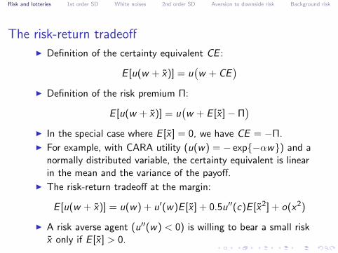
I Definition of the certainty equivalent CE :
E [u(w + x)] = u(w + CE
)I Definition of the risk premium Π:
E [u(w + x)] = u(w + E [x ]− Π
)I In the special case where E [x ] = 0, we have CE = −Π.
I For example, with CARA utility (u(w) = − exp{−αw}) and anormally distributed variable, the certainty equivalent is linearin the mean and the variance of the payoff.
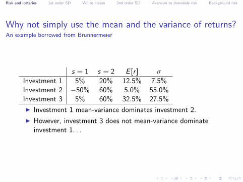
I Investment 1 mean-variance dominates investment 2.
I However, investment 3 does not mean-variance dominateinvestment 1. . .
Risk and lotteries 1st order SD White noises 2nd order SD Aversion to downside risk Background risk
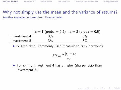
Why not simply use the mean and the variance of returns?Another example borrowed from Brunnermeier
s = 1 (proba = 0.5) s = 2 (proba = 0.5)
Investment 4 3% 5%Investment 5 3% 8%
I Sharpe ratio: commonly used measure to rank portfolios:
SR =E [r ]− rf
σr
I For rf = 0, investment 4 has a higher Sharpe ratio thaninvestment 5 !
Risk and lotteries 1st order SD White noises 2nd order SD Aversion to downside risk Background risk
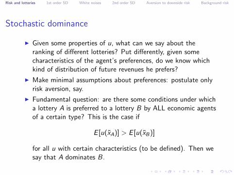
Stochastic dominance
I Given some properties of u, what can we say about theranking of different lotteries? Put differently, given somecharacteristics of the agent’s preferences, do we know whichkind of distribution of future revenues he prefers?
I Make minimal assumptions about preferences: postulate onlyrisk aversion, say.
I Fundamental question: are there some conditions under whicha lottery A is preferred to a lottery B by ALL economic agentsof a certain type? This is the case if
E [u(xA)] > E [u(xB)]
for all u with certain characteristics (to be defined). Then wesay that A dominates B.
Risk and lotteries 1st order SD White noises 2nd order SD Aversion to downside risk Background risk
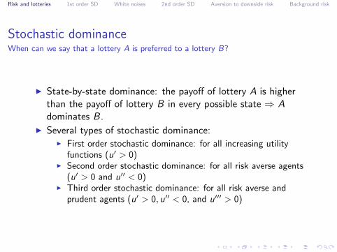
Stochastic dominanceWhen can we say that a lottery A is preferred to a lottery B?
I State-by-state dominance: the payoff of lottery A is higherthan the payoff of lottery B in every possible state ⇒ Adominates B.
I Several types of stochastic dominance:I First order stochastic dominance: for all increasing utility
functions (u′ > 0)I Second order stochastic dominance: for all risk averse agents
(u′ > 0 and u′′ < 0)I Third order stochastic dominance: for all risk averse and
prudent agents (u′ > 0, u′′ < 0, and u′′′ > 0)
Risk and lotteries 1st order SD White noises 2nd order SD Aversion to downside risk Background risk
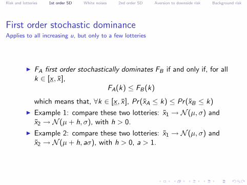
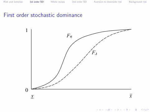
First order stochastic dominanceApplies to all increasing u, but only to a few lotteries
I FA first order stochastically dominates FB if and only if, for allk ∈ [x , x ],
FA(k) ≤ FB(k)
which means that, ∀k ∈ [x , x ], Pr(xA ≤ k) ≤ Pr(xB ≤ k)
I Example 1: compare these two lotteries: x1 → N (µ, σ) andx2 → N (µ+ h, σ), with h > 0.
I Example 2: compare these two lotteries: x1 → N (µ, σ) andx2 → N (µ+ h, aσ), with h > 0, a > 1.
Risk and lotteries 1st order SD White noises 2nd order SD Aversion to downside risk Background risk
First order stochastic dominance
)�
[ [
0
1)�
Risk and lotteries 1st order SD White noises 2nd order SD Aversion to downside risk Background risk
First order stochastic dominanceApplies to all increasing u, but only to a few lotteries
I Intuitive interpretation: shift in probability weights.
I Criterion which applies to all economic agents who prefermore money to less (whether they are risk averse or not), butwhich only enables to compare a narrow subset of lotteries. . .
I FOSD is not the same as state-by-state dominance. Example:the payoffs are given (say, $1, $2, $3), and different lotteriesoffer these payoffs with different probabilities ⇒ we may haveFOSD, but not state-by-state dominance.
Risk and lotteries 1st order SD White noises 2nd order SD Aversion to downside risk Background risk
White noisesA “pure”, zero-mean risk
I Which changes in risk (i.e., in the probability distribution ofthe payoff) decrease the expected utility of the lottery for allrisk averse agents?
I Consider two lotteries:I Lottery A yields 1 with proba 0.5 and 3 with proba 0.5.I Lottery B yields 1 with proba 0.5, 2 with proba 0.25, and 4
with proba 0.25.I Same expected payoff (2).
I Lottery B is a compound lottery: playing lottery B isequivalent to playing lottery A and another lottery withzero-mean. It is equivalent to adding a white noise to lotteryA.
Risk and lotteries 1st order SD White noises 2nd order SD Aversion to downside risk Background risk
White noisesRisk averse agents are averse to white noises
I Adding a white noise (lottery with zero mean) to any lotteryreduces the expected utility of all risk averse agents.
I Another example:
Ex
[Eε[u(x + ε)
]]< Ex
[u(x + Eε[ε])
]= Ex
[u(x)
]The inequality follows once again from Jensen inequality.
I Whenever we need to compare two lotteries, can we show thatone lottery is equal to the other compounded by a whitenoise?
I Two types of white noises (in any case, E [ε|x = x ] = 0 ∀x):I The existence of the white noise ε is conditional on the
outcome x of the first lottery → example on the precedingslide.
I The existence of the white noise ε is unconditional on theoutcome x of the first lottery → example on this slide.
Risk and lotteries 1st order SD White noises 2nd order SD Aversion to downside risk Background risk
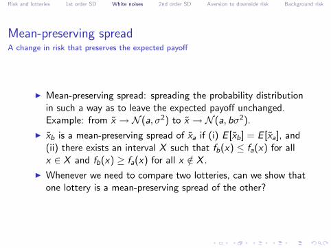
Mean-preserving spreadA change in risk that preserves the expected payoff
I Mean-preserving spread: spreading the probability distributionin such a way as to leave the expected payoff unchanged.Example: from x → N (a, σ2) to x → N (a, bσ2).
I xb is a mean-preserving spread of xa if (i) E [xb] = E [xa], and(ii) there exists an interval X such that fb(x) ≤ fa(x) for allx ∈ X and fb(x) ≥ fa(x) for all x /∈ X .
I Whenever we need to compare two lotteries, can we show thatone lottery is a mean-preserving spread of the other?
Risk and lotteries 1st order SD White noises 2nd order SD Aversion to downside risk Background risk
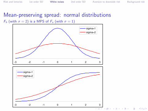
Mean-preserving spread: normal distributionsFb (with σ = 2) is a MPS of Fa (with σ = 1)
-3 -2 -1 0 1 2 3
sigma=1
sigma=2
-3 -2 -1 0 1 2 3
sigma=1
sigma=2
Risk and lotteries 1st order SD White noises 2nd order SD Aversion to downside risk Background risk
Mean-preserving spread and second-order stochasticdominance (1)
I Assume that FB is a mean-preserving spread (MPS) of FA.This implies, by definition of a MPS:∫ x
xx [fB(x)− fA(x)]dx = 0 (1)
I Integrate by parts the LHS, remembering that∫ x
xw ′(x)v(x)dx =
[w(x)v(x)
]xx−∫ x
xw(x)v ′(x)dx
I Here, set w ′(x) = fB(x)− fA(x) and v(x) = x . We get∫ x
xx [fB(x)−fA(x)]dx =
[[FB(x)−FA(x)]x
]xx−∫ x
x[FB(x)−FA(x)]dx
(2)
Risk and lotteries 1st order SD White noises 2nd order SD Aversion to downside risk Background risk
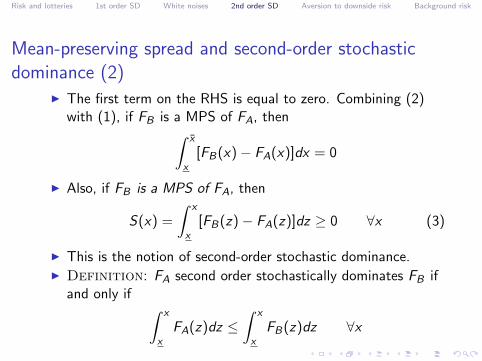
Mean-preserving spread and second-order stochasticdominance (2)
I The first term on the RHS is equal to zero. Combining (2)with (1), if FB is a MPS of FA, then∫ x
x[FB(x)− FA(x)]dx = 0
I Also, if FB is a MPS of FA, then
S(x) =
∫ x
x[FB(z)− FA(z)]dz ≥ 0 ∀x (3)
I This is the notion of second-order stochastic dominance.I Definition: FA second order stochastically dominates FB if
and only if ∫ x
xFA(z)dz ≤
∫ x
xFB(z)dz ∀x
Risk and lotteries 1st order SD White noises 2nd order SD Aversion to downside risk Background risk
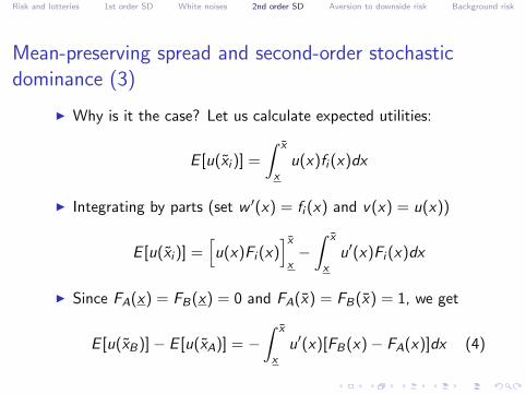
Mean-preserving spread and second-order stochasticdominance (3)
I Why is it the case? Let us calculate expected utilities:
E [u(xi )] =
∫ x
xu(x)fi (x)dx
I Integrating by parts (set w ′(x) = fi (x) and v(x) = u(x))
E [u(xi )] =[u(x)Fi (x)
]xx−∫ x
xu′(x)Fi (x)dx
I Since FA(x) = FB(x) = 0 and FA(x) = FB(x) = 1, we get
E [u(xB)]− E [u(xA)] = −∫ x
xu′(x)[FB(x)− FA(x)]dx (4)
Risk and lotteries 1st order SD White noises 2nd order SD Aversion to downside risk Background risk
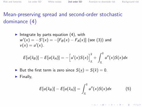
Mean-preserving spread and second-order stochasticdominance (4)
I Integrate by parts equation (4), withw ′(x) = −S ′(x) = −[FB(x)− FA(x)] (see (3)) andv(x) = u′(x).
E [u(xB)]− E [u(xA)] = −[u′(x)S(x)
]xx
+
∫ x
xu′′(x)S(x)dx
I But the first term is zero since S(x) = S(x) = 0.
I Finally,
E [u(xB)]− E [u(xA)] =
∫ x
xu′′(x)S(x)dx (5)
Risk and lotteries 1st order SD White noises 2nd order SD Aversion to downside risk Background risk
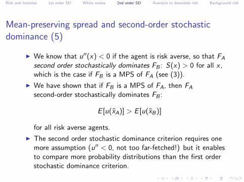
Mean-preserving spread and second-order stochasticdominance (5)
I We know that u′′(x) < 0 if the agent is risk averse, so that FA
second order stochastically dominates FB : S(x) > 0 for all x ,which is the case if FB is a MPS of FA (see (3)).
I We have shown that if FB is a MPS of FA, then FA
second-order stochastically dominates FB :
E [u(xA)] > E [u(xB)]
for all risk averse agents.
I The second order stochastic dominance criterion requires onemore assumption (u′′ < 0, not too far-fetched!) but it enablesto compare more probability distributions than the first orderstochastic dominance criterion.
Risk and lotteries 1st order SD White noises 2nd order SD Aversion to downside risk Background risk
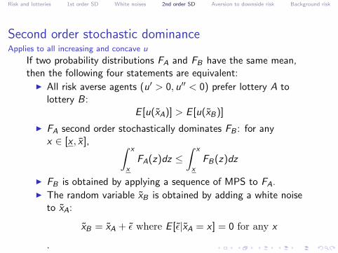
Second order stochastic dominanceApplies to all increasing and concave u
If two probability distributions FA and FB have the same mean,then the following four statements are equivalent:
I All risk averse agents (u′ > 0, u′′ < 0) prefer lottery A tolottery B:
E [u(xA)] > E [u(xB)]
I FA second order stochastically dominates FB : for anyx ∈ [x , x ], ∫ x
xFA(z)dz ≤
∫ x
xFB(z)dz
I FB is obtained by applying a sequence of MPS to FA.I The random variable xB is obtained by adding a white noise
to xA:
xB = xA + ε where E [ε|xA = x ] = 0 for any x
.
Risk and lotteries 1st order SD White noises 2nd order SD Aversion to downside risk Background risk
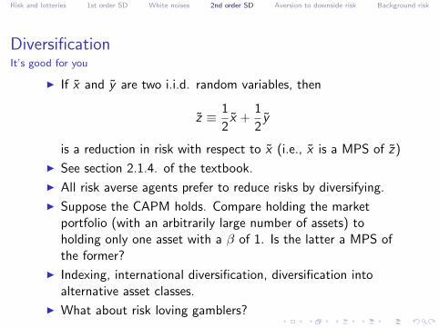
DiversificationIt’s good for you
I If x and y are two i.i.d. random variables, then
z ≡ 1
2x +
1
2y
is a reduction in risk with respect to x (i.e., x is a MPS of z)
I See section 2.1.4. of the textbook.
I All risk averse agents prefer to reduce risks by diversifying.
I Suppose the CAPM holds. Compare holding the marketportfolio (with an arbitrarily large number of assets) toholding only one asset with a β of 1. Is the latter a MPS ofthe former?
I Indexing, international diversification, diversification intoalternative asset classes.
I What about risk loving gamblers?
Risk and lotteries 1st order SD White noises 2nd order SD Aversion to downside risk Background risk
Aversion to downside risk
I Do you prefer your wealth to be random when you are wealthyor when you are poor?
I With lottery a, you have 1000 + ε with probability 0.5 and2000 with probability 0.5.
I With lottery b, you have 1000 with probability 0.5 and2000 + ε with probability 0.5.
I Experiments: people tend to prefer lottery b: aversion todownside risk.
Risk and lotteries 1st order SD White noises 2nd order SD Aversion to downside risk Background risk
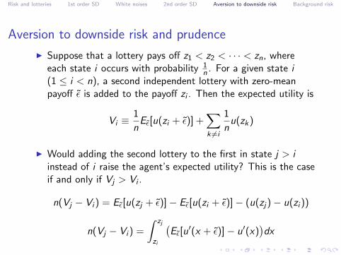
Aversion to downside risk and prudence
I Suppose that a lottery pays off z1 < z2 < · · · < zn, whereeach state i occurs with probability 1
n . For a given state i(1 ≤ i < n), a second independent lottery with zero-meanpayoff ε is added to the payoff zi . Then the expected utility is
Vi ≡1
nEε[u(zi + ε)] +
∑k 6=i
1
nu(zk)
I Would adding the second lottery to the first in state j > iinstead of i raise the agent’s expected utility? This is the caseif and only if Vj > Vi .
Risk and lotteries 1st order SD White noises 2nd order SD Aversion to downside risk Background risk
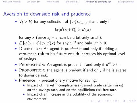
Aversion to downside risk and prudenceI Vj > Vi for any collection of {zi}i=1,...n if and only if
Eε[u′(x + ε)] > u′(x)
for any x (since zj − zi can be arbitrarily small).I Eε[u
′(x + ε)] > u′(x) for any x if and only u′′′ > 0.I Definition: An agent is prudent if and only if adding a
zero-mean risk to his future wealth increases his optimal levelof savings.
I Proposition: An agent is prudent if and only if u′′′ > 0.I Proposition: the agent is prudent if and only if he is averse
to downside risk.I Prudence ⇒ precautionary motive for saving.
I Impact of market incompleteness (cannot trade certain risks)on the savings rate, and on the equilibrium risk-free rate.
I Impact of an increase in the volatility of the economicenvironment.
Risk and lotteries 1st order SD White noises 2nd order SD Aversion to downside risk Background risk
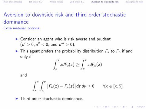
Aversion to downside risk and third order stochasticdominanceExtra material, optional
I Consider an agent who is risk averse and prudent(u′ > 0, u′′ < 0, and u′′′ > 0).
I This agent prefers the probability distribution Fa to Fb if andonly if ∫ x
xzdFa(z) ≥
∫ x
xzdFb(z)
and ∫ x
x
∫ y
x
[Fb(z)− Fa(z)
]dz dy ≥ 0 ∀x ∈ [x , x ]
I Third order stochastic dominance.
Risk and lotteries 1st order SD White noises 2nd order SD Aversion to downside risk Background risk
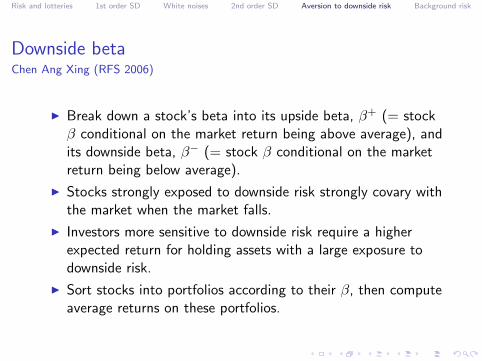
Downside betaChen Ang Xing (RFS 2006)
I Break down a stock’s beta into its upside beta, β+ (= stockβ conditional on the market return being above average), andits downside beta, β− (= stock β conditional on the marketreturn being below average).
I Stocks strongly exposed to downside risk strongly covary withthe market when the market falls.
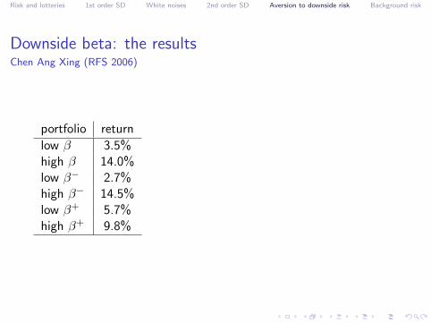
I Investors more sensitive to downside risk require a higherexpected return for holding assets with a large exposure todownside risk.
I Sort stocks into portfolios according to their β, then computeaverage returns on these portfolios.
Risk and lotteries 1st order SD White noises 2nd order SD Aversion to downside risk Background risk
Downside beta: the resultsChen Ang Xing (RFS 2006)
Risk and lotteries 1st order SD White noises 2nd order SD Aversion to downside risk Background risk
Several degrees of risk increasesTo summarize. . .
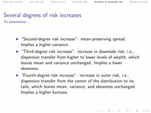
I “Second-degree risk increase”: mean-preserving spread.Implies a higher variance.
I “Third-degree risk increase”: increase in downside risk, i.e.,dispersion transfer from higher to lower levels of wealth, whichleaves mean and variance unchanged. Implies a lowerskewness.
I “Fourth-degree risk increase”: increase in outer risk, i.e.,dispersion transfer from the center of the distribution to itstails, which leaves mean, variance, and skewness unchanged.Implies a higher kurtosis.
Risk and lotteries 1st order SD White noises 2nd order SD Aversion to downside risk Background risk
Taking multiple risks
I Suppose that I offer you the following gamble: I will toss afair coin, you earn $110 if it’s heads, you lose $100 if it’s tails.
I Do you accept this bet?
I Does your attitude change if you bet twice instead (on thesame bet)? What about a hundred times?
Risk and lotteries 1st order SD White noises 2nd order SD Aversion to downside risk Background risk
Taking multiple risks
I Be careful not to misinterpret the law of large numbers.
I Risk is reduced if instead of being exposed to one risk of size1, the agent is exposed to n i.i.d. risks of size 1
n .
I Risk is not reduced is the agent is exposed to two (or ahundred) sources of risk instead of one.
I In the example above, the gamble would become moreappealing if the size of the bet diminished in proportion to thenumber of bets: for n bets, the gain (resp. loss) on each betwould be 110
n (resp. 100n ).
I In this case with the subdivision of the bet size, in the limit,as the number of bets n tends to infinity, the law of largenumbers indeed applies and the average net gain approaches$5.
Risk and lotteries 1st order SD White noises 2nd order SD Aversion to downside risk Background risk
The tempering effect of background riskI Intuitively, being exposed to one risk should lower the
willingness of an economic agent to bear another risk.I Definition: Preferences are characterized by risk
vulnerability if the presence of an exogenous background riskwith nonpositive mean (including a pure risk) increases theaversion to other independent risks.
I Definition: Risk aversion is standard if absolute riskaversion and absolute prudence are decreasing with wealth.
I Proposition: Standardness is a sufficient condition for riskvulnerability.
I Proposition: Preferences are risk vulnerable if absolute riskaversion is decreasing and convex. (The Proof follows)
I This condition means that the risk premium is decreasing withwealth at a decreasing rate.1 In particular, absolute riskaversion is decreasing and convex with CRRA utility.
1Notice that absolute risk aversion cannot be positive, decreasing andconcave for all levels of wealth.
Risk and lotteries 1st order SD White noises 2nd order SD Aversion to downside risk Background risk
Proof of the second Proposition
I Preferences are risk vulnerable iff the indirect utility functionis more concave than u, for any risk x with nonpositive mean:
−E [u′′(z + x)]
E [u′(z + x)]≥ −u′′(z)
u′(z)for all z
E [A(z + x)u′(z + x)] ≥ A(z)E [u′(z + x)] for all z
I To get this result, first note that DARA implies thatcov(A(z + x), u′(z + x)) ≥ 0 so that
E [A(z + x)u′(z + x)] ≥ E [A(z + x)]E [u′(z + x)]
I Furthermore, if absolute risk aversion is convex, then Jenseninequality implies that
E [A(z + x)] ≥ A(z + E [x ]) ≥ A(z)
Risk and lotteries 1st order SD White noises 2nd order SD Aversion to downside risk Background risk
The tempering effect of background risk: implications andapplications
I What is the impact on risk taking (and on the market price ofrisk) of introducing or raising healthcare insurance,unemployment insurance, disability insurance?
I What about a change in the probability of a deep recessionwhich would significantly lower labor incomes and raise theprobability of unemployment?
I What about a terrorist threat, the possibility of a pandemic,or of a shortage of food or water?
I The Great Moderation and the market price of risk from 2003to Q2 2007.
Risk and lotteries 1st order SD White noises 2nd order SD Aversion to downside risk Background risk
ExercisesHomework
I 2.1
I 2.5
I Exercises on zonecours.
Risk and lotteries 1st order SD White noises 2nd order SD Aversion to downside risk Background risk
I Acknowledgements: Some sources for this series of slidesinclude:
I The slides of Martin Boyer, for the same course at HECMontreal.
I Asset Pricing, by John H. Cochrane.I Finance and the Economics of Uncertainty, by Gabrielle
Demange and Guy Laroque.I The Economics of Risk and Time, by Christian Gollier.