Risk Premia in Structured Credit Derivatives Andreas Eckner ∗ First version: September 2, 2007 Current version: May 9, 2010 Abstract During the past couple of years much research effort has been devoted to ex- plaining the spread of corporate bonds over Treasuries. On the other hand, rela- tively little is known about the spread components of structured credit products. This paper shows that such securities compensate investors for expected losses due to defaults, pure jump-to-default risk, correlation risk, as well as the risk of firm-specific and market-wide adverse changes in credit conditions. We provide a framework that allows a decomposition of ”structured” credit spreads, and we apply this decomposition to CDX index tranches. Keywords: credit risk, correlated default, structured credit derivatives, affine jump diffusion, tranche spread decomposition, portfolio loss decomposition * Department of Statistics, Stanford University. All comments are welcome via email: [email protected]. The source code of the implementation is available at http://www.eckner.com/research.html. I would like to thank Xiaowei Ding, Kay Giesecke, Tze Leung Lai, Allan Mortensen and George Papanicolaou for helpful comments and remarks, and especially Darrell Duffie for frequent discussions. I am grateful to Citi, Markit and Morgan Stanley for providing historical CDX index and tranche spreads, as well as Barclays Capital and Markit for providing historical CDS spread data.
Transcript
Risk Premia in Structured Credit Derivatives
Andreas Eckner∗
First version: September 2, 2007Current version: May 9, 2010
Abstract
During the past couple of years much research effort has been devoted to ex-plaining the spread of corporate bonds over Treasuries. On the other hand, rela-tively little is known about the spread components of structured credit products.This paper shows that such securities compensate investors for expected lossesdue to defaults, pure jump-to-default risk, correlation risk, as well as the risk offirm-specific and market-wide adverse changes in credit conditions. We providea framework that allows a decomposition of ”structured” credit spreads, and weapply this decomposition to CDX index tranches.
∗Department of Statistics, Stanford University. All comments are welcome viaemail: [email protected]. The source code of the implementation is available athttp://www.eckner.com/research.html. I would like to thank Xiaowei Ding, Kay Giesecke, TzeLeung Lai, Allan Mortensen and George Papanicolaou for helpful comments and remarks, andespecially Darrell Duffie for frequent discussions. I am grateful to Citi, Markit and Morgan Stanleyfor providing historical CDX index and tranche spreads, as well as Barclays Capital and Markit forproviding historical CDS spread data.
1 Introduction
We focus on the investment-grade CDX family of structured credit products, for theirentire trading history up to November 2006. These products allocate default losses on aportfolio of US corporate debt of 125 firms, equally weighted, to a list of tranches. Thefirst-loss, or “equity” tranche, for example, is allocated default losses as they occur, up tothe 3% of the total notional amount of the 125-name portfolio. The other tranches coverlosses, respectively between 3 and 7% of notional (”junior mezzanine”), between 7 and10% of notional (”mezzanine”), between 10 and 15% of notional (“senior mezzanine”),between 15 and 30% of notional (”senior”), and between 30 and 100% of the notional(“super senior”).
We find that investors in the CDX first-loss tranche on average bear about 93.3%of the expected losses on the underlying portfolio of corporate debt, and receive about77.0% of the total compensation for bearing portfolio losses. On the other hand, in-vestors in the senior tranche, on average, bear about 0.2% of expected default losses onthe underlying portfolio, and receive about 2% of the total compensation. In terms ofthe ratio, on average, of compensation rate per unit of expected loss, the first-loss piececarries a risk premium of 3.9, whereas the most senior tranches offer a risk premium ofabout 50. This extreme difference in risk premia is natural given that the most seniortranches bear losses only when there is a significant ”meltdown” in corporate perfor-mance. As opposed to the finding of Coval, Jurek, and Stafford (2007) that investors donot demand much compensation for this extremely systematic risk, there does seem tobe evidence of significant compensation for the systematic nature of this risk.
Using the methods developed in this paper, we are able to break down the com-pensation for bearing default risk into several components: compensation for actualexpected losses, systematic risk, firm-specific risk, correlation risk, and pure jump-to-default (JTD) risk.1 The various tranches have different rates of compensation per unitof expected loss because they carry these various types of risks in different proportions toeach other. For example, the equity tranche is allocated 81.7% of the total compensationfor firm-specific risk in the underlying portfolio of debt, but carries only 32.0% of thetotal compensation for systematic risk. The senior tranche, on the other hand, is allo-cated only 0.2% of the total compensation for firm-specific risk, but carries a relativelylarge fraction, 9.9%, of the total compensation for systematic risk.
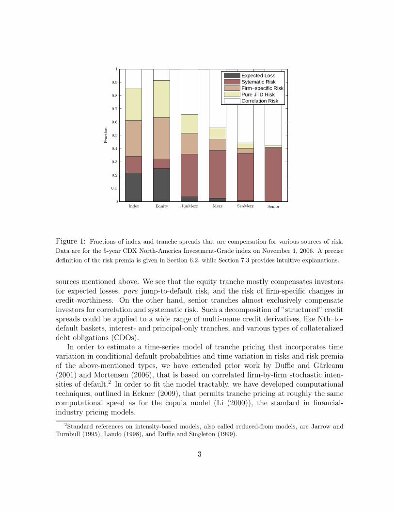
For the 5-year CDX.NA.IG index on November 1, 2006, Figure 1 shows for eachtranche the fraction of its compensation that can be attributed to each of the five risk
1The latter component is sometimes called timing risk, or portfolio sampling risk. Compensationfor correlation risk premium and pure jump-to-default risk would not be separately identifiable in aunivariate setting. Hence, in recent research on the components of corporate bond and CDS spreads,the sum of these two risk premia is simply called the jump-to-default risk premium. See for exampleDriessen (2005), Berndt, Douglas, Duffie, Ferguson, and Schranz (2005), Amato (2005), Amato andRemolona (2005), and Saita (2006).
Figure 1: Fractions of index and tranche spreads that are compensation for various sources of risk.
Data are for the 5-year CDX North-America Investment-Grade index on November 1, 2006. A precise
definition of the risk premia is given in Section 6.2, while Section 7.3 provides intuitive explanations.
sources mentioned above. We see that the equity tranche mostly compensates investorsfor expected losses, pure jump-to-default risk, and the risk of firm-specific changes incredit-worthiness. On the other hand, senior tranches almost exclusively compensateinvestors for correlation and systematic risk. Such a decomposition of ”structured” creditspreads could be applied to a wide range of multi-name credit derivatives, like Nth–to-default baskets, interest- and principal-only tranches, and various types of collateralizeddebt obligations (CDOs).
In order to estimate a time-series model of tranche pricing that incorporates timevariation in conditional default probabilities and time variation in risks and risk premiaof the above-mentioned types, we have extended prior work by Duffie and Garleanu(2001) and Mortensen (2006), that is based on correlated firm-by-firm stochastic inten-sities of default.2 In order to fit the model tractably, we have developed computationaltechniques, outlined in Eckner (2009), that permits tranche pricing at roughly the samecomputational speed as for the copula model (Li (2000)), the standard in financial-industry pricing models.
2Standard references on intensity-based models, also called reduced-from models, are Jarrow andTurnbull (1995), Lando (1998), and Duffie and Singleton (1999).
3
The remainder of this section discusses applications for our work and related lit-erature. We also describe the most common credit derivative contracts, and the datasources used for our analysis. Section 2 presents descriptive statistics of the historicalprice behavior of some credit derivatives. Section 3 introduces the model for defaulttimes and describes the pricing of credit derivatives in this framework. Section 5 ex-amines the model fit to the time series of credit tranche spreads. Section 6 introducesa joint model for physical and risk-neutral default intensities, while Section 7 presentsthe fitted model and a decomposition of credit tranche spreads and portfolio defaultcompensation. Section 8 concludes.
1.1 Applications
A better understanding of what drives changes in the price of credit risky securitiesshould be of interest to a variety of researchers and practitioners. Asset pricing re-searchers typically try to link the sensitivity of security prices to certain state variables.The findings in this paper indicate that for some credit derivative contracts, changes inrisk premia over time might play a more important role than has traditionally been as-signed to them, especially for senior tranche spreads, which heavily depend on perceivedtail risk. See also Collin-Dufresne, Goldstein, and Martin (2001), who find that variousproposed proxies for changes in default probabilities and recovery rates can explain onlyabout 25 percent of observed credit spread changes.
Investors in single-name and structured credit products would like to better under-stand the types of risks to which they are exposed to, and to quantify the extent to whichthey are being compensated for these risks. The decomposition of credit tranche spreadsin this paper indicates how a linear combination of credit tranches might allow to isolatethe exposure to a certain type of risk, for example pure jump-to-default risk, which in thepast has carried a rather large risk premium.3 Coval, Jurek, and Stafford (2007) arguethat investors in senior CDO tranches underprice systematic risks by solely relying oncredit ratings for the purpose of making investment decisions. We find that, at least forcorporate credits, investors are reasonably aware, in terms of compensation demandedabove and beyond expected losses, about the differences in the risks between structuredand single-name credit products, although in our framework we cannot preclude thatinvestors are at least partially oblivious about these differences.
Finally, a better understanding of structured credit products should be of interest todealers in these securities, since it would allow them to better hedge and quantify theirinventory risk. When order flow becomes imbalanced, as in May 2005 and July/August
3The large size of this risk premium has led to the term ”credit spread puzzle”, see for exampleDriessen (2005), Berndt, Douglas, Duffie, Ferguson, and Schranz (2005), Chen, Collin-Dufresne, andGoldstein (2006) and Saita (2006). In our framework, the pure JTD risk premium accounts for roughlytwo thirds of the total JTD risk premium, so that the puzzle is somewhat reduced, but remains intactfor highly rated issuers.
4
2007, it is important for liquidity providers to assess whether this imbalance is causedby informed or uniformed traders, so that they can quote more competitive spreads andsupport an orderly working of the credit markets.
1.2 Related Literature
There exists a vast literature on corporate default risk, initiated by Altman (1968).However, due to computational challenges, most research on the dynamics of physical(or real-world) default intensities (in the following denoted by λP
i ) is still quite recent.Duffie, Saita, and Wang (2007) model a firm’s default intensity as dependent on a setof firm-specific and macroeconomic covariates, of which distance-to-default, which is avolatility-adjusted measure of leverage, has the most influence. They estimate the time-series dynamics of all covariates and therefore arrive at a fully dynamic model for a firm’sdefault intensity and default time. Duffie, Eckner, Horel, and Saita (2009) extend thismodel by including a dynamic frailty variable, a time-varying latent factor that affectsthe default risk of all companies. They find that such a latent factor is important forexplaining the tendency of corporate defaults to cluster over time, as in 1989-1990 and2001-2002, and for obtaining a realistic level of default correlation in intensity-basedmodels.
The recent emergence of a wide array of single-name and structured credit productshas made available a tremendous amount of information about investors’ risk preferencesin the credit markets.4 Modeling the dynamics of risk-neutral default intensities (in thefollowing denoted by λQ
i ) therefore is currently an extremely active research area. See forexample Duffie and Garleanu (2001), Giesecke and Goldberg (2005), Errais, Giesecke,and Goldberg (2006), Joshi and Stacey (2006), Longstaff and Rajan (2008), Mortensen(2006), Papageorgiou and Sircar (2007), and Eckner (2009). Schneider, Sogner, and Veza(2007) and Feldhutter (2007) examine both the risk-neutral and ”physical” dynamics ofλQ
i .Nevertheless, a joint framework for the multivariate dynamics of physical and risk-
neutral default intensities is still limited. Recent research in this area includes Berndt,Douglas, Duffie, Ferguson, and Schranz (2005), Amato (2005), Amato and Remolona(2005), and Saita (2006). Our paper continues this line of work by incorporating CDXtranche spread data into the analysis, which allows us to better pin down the multivariatedynamics of risk-neutral default intensities and to quantify certain risk premia that areunique to a multivariate setting.
4Although corporate bond spreads also contain at least the single-name information, they tend toreflect tax and liquidity effects, see Elton, Gruber, Agrawal, and Mann (2001), Driessen (2005), andLongstaff, Mithal, and Neis (2005). On the other hand, credit default swap spreads are usually regardedas a quite pure measure of perceived default risk. They allow to short credit risk much more easily andcheaper than using corporate bonds, and have standardized maturity dates and credit event triggers,which enhances their liquidity.
5
1.3 Credit Derivative Contracts
A credit derivative is a contract whose payoff is linked to the creditworthiness of one ormore obligations. This section summarizes the features of the three most common typesfor corporate credit risk.
Credit Default Swaps. By far the most common credit derivative is the creditdefault swap (CDS). It is an agreement between a protection buyer and a protectionseller, whereby the buyer pays a periodic fee in return for a contingent payment by theseller upon a credit event, such as bankruptcy or “failure to pay”, of a reference entity.The contingent payment usually replicates the loss incurred by a creditor of the referenceentity in the event of its default. See, for example, Duffie (1999).
Credit Indices. A credit index contract allows an investor to either buy or sellprotection on a basket of reference entities, and therefore closely resembles a portfo-lio of CDS contracts. For example, the CDX.NA.IG (for CDS index, North America,Investment Grade) contract provides equally-weighted default protection on 125 NorthAmerican investment-grade rated issuers. For a more detailed description see the ’CreditDerivatives Handbook’ (2006) by Merrill Lynch.
Credit Tranches. A credit tranche allows an investor to gain a specified exposureto the credit risk of the underlying portfolio, while in return receiving periodic couponpayments. Losses due to credit events in the underlying portfolio are allocated first tothe lowest tranche, known as the equity tranche, and then to successively prioritizedtranches. The risk of a tranche is determined by the attachment point of the tranche,which defines the point at which losses in the underlying portfolio begin to reduce thetranche notional, and the detachment point, which defines the point at which losses inthe underlying portfolio reduce the tranche notional to zero. The buyer of protectionmakes coupon payments on the notional amount of the remaining size of the tranche,which is the initial tranche size less losses due to defaults. This structure is illustratedin Table 1 for the CDX.NA.IG index.
The coupon payments for these three contracts are typically made quarterly, on theIMM dates, which are the 20th of March, June, September, and December, unless thisdate is a holiday, in which case the payment is made on the next business day. If acontract is entered in between two such dates, the buyer of protection receives from theseller of protection the accrued premium since the last IMM date.
6
Tranche Attachment Point Detachment Point Quote ConventionEquity 0% 3% 500 bps running + upfrontJunior Mezzanine 3% 7% all runningMezzanine 7% 10% all runningSenior Mezzanine 10% 15% all runningSenior 15% 30% all runningSuper Senior 30% 100% all running
Table 1: Tranche structure of the CDX.NA.IG index, which has 125 equally weighted North-American
investment-grade issuers in the underlying portfolio.
1.4 Data Sources
Citi and Morgan Stanley provided 5, 7, and 10-year CDX.NA.IG index and tranche bid-and ask-spreads. Markit provided 5, 7, and 10-year CDX.NA.IG tranche mid-marketspreads, and 1, 5, 7, and 10-year CDS mid-market spreads for the CDX.NA.IG members.
We used 3-month, 6-month, 9-month, 1-year, 2-year, ..., 10-year US LIBOR swaprates to estimate the discount function Bt (T ) at each point in time t. Specifically, forthese standard maturities we used swap rates from the Bloomberg system, while fornon-standard maturities we used cubic-spline interpolation of implied forward rates todetermine the spot rate. Swap rates are widely regarded as the best measure of fundingcosts for banks - the biggest participant in the market for synthetic credit derivatives -over various time horizons.
2 Descriptive Analysis
This section gives a brief overview of historical CDX.NA.IG index and tranche spreadsand provides some descriptive statistics. In the subsequent analysis we will frequentlyrefer to the credit market events mentioned here. Unless mentioned otherwise, marketprices refer to mid-market prices for the remainder of the paper.
Figure 2 shows the historical spread for the three standard maturities of the CDX.NA.IGindex. We see that credit spreads have narrowed considerably between October 2003and November 2006, although this narrowing was sharply interrupted in May 2005. Cor-responding tightenings of spreads affected the tranches making up the index. However,there are some peculiarities in the history of tranche spreads that are worth mentioningin order to interpret the time-series results in Section 5 and 7.
A principal component analysis of the standardized daily tranche spread changes(∆Sj/
√V ar (∆Sj) : 1 ≤ j ≤ 5) with j = 1 for the equity tranche, up to j = 5 for the
Figure 2: Historical spread of the on-the-run CDX.NA.IG index for maturity equal to 5 years (solid
line), 7 years (dashed line) and 10 years (dotted line). The vertical lines represent the bi-annual roll-over
dates.
senior tranche, gives the first three principal component weighting vectors
PC1 =
0.400.480.480.450.42
, PC2 =
−0.840.050.300.44
−0.07
, PC3 =
−0.22−0.32−0.22−0.08
0.89
. (1)
The first three principal components explain 76%, 10%, and 8% of the variance of changesin tranche spreads, respectively. As can be seen from (1), the first principal componentreflects a market-wide increase of credit risk, the second component reflects an increaseof tail risk at moderate loss levels (mezzanine and senior mezzanine tranche), and thethird component corresponds to an increase of tail risk at very extreme loss levels (seniortranche). Figure 3 shows the historical evolution of the first three principal componentsof standardized tranche spread changes between October 2003 and April 2006.5 The
5We define the evolution of a principal component as the performance of a portfolio of credit trancheswith position sizes proportional to the principal component entries, normalized by tranche notional sizeand tranche spread volatility.
8
-60
-50
-40
-30
-20
-10
0
10
20
Sep03 Feb04 Aug04 Feb05 Jul05 Dec05 Jun06 Nov06
Cum
ula
tive
Ret
urn
ofP
rinci
palC
om
ponen
tPort
folio
Figure 3: Historical evolution of the first three principal component portfolios (solid, dashed and
dotted line, respectively) for the tranche spreads of the 5-year CDX.NA.IG index.
downward trend in the first principal component portfolio simply reflects the fact thatcredit spreads have narrowed considerably during this time period. The evolution ofthe second and third component shows that perceived default risk at extreme loss levelsincreased dramatically in May 2006, while perceived default risk at moderate loss levelsapparently collapsed. This shock to the credit market was caused by the same-daydowngrades of Ford Motor Company and General Motors Corp. to a sub-investment-grade rating (that is, lower than BBB−), which led to selling of bonds of these firms byinvestors who are allowed to hold only investment-grade rated securities. At the sametime, a partial take-over attempt of General Motors Corp. led to a sharp increase inits share price. The combination of these two events ”caused the relationship betweenprices of certain assets to change in an unexpected way”. (See BIS Quarterly Review,June 2005, for a detailed discussion.)
Table 2 provides some summary statistics about the riskiness of reference entitiesthat were part of the CDX.NA.IG index at least once between September 2004 andNovember 2006.
Table 2: Summary statistics on the default risk of reference entities that were part of the CDX.NA.IG
index at least once between September 21, 2004, and November 30, 2006. Historical 1-year and 5-year
default probabilities were taken from Moody’s Investor Service, ’Historical Default Rates of Corporate
Bond Issuers, 1920-1999’.
3 Model Setup
This section describes a model for the joint distribution of various obligor default timesunder a risk-neutral probability measure. The setup is the same as in Eckner (2009),which in turn is similar to the one of Duffie and Garleanu (2001) and Mortensen (2006).
To this end, we fix a filtered probability space (Ω,F , (Ft) , P) satisfying the usualconditions.6 Up to purely technical conditions,7 the absence of arbitrage implies theexistence of an equivalent martingale measure Q, such that the price at time t of asecurity paying an amount Z at a bounded stopping time τ > t is given by
Vt = EQt
(e−
∫ τ
trsdsZ
),
where r is the short-term interest rate and EQt denotes expectation under Q conditional
on all available information up to time t.Under the equivalent martingale measure Q, for each individual firm i, a default time
τ i is modeled using Cox processes, also known as doubly stochastic Poisson processes.8
Specifically, the default intensity of obligor i is a non-negative real-valued progressivelymeasurable stochastic process, which will be defined below. Conditional on the intensitypath λQ
it : t ≥ 0, the default time τ i is taken to be the first jump time of an inhomo-geneous Poisson process with intensity λQ
i . In particular, the default times of any setof firms are conditionally independent given the intensity paths, so that correlation ofdefault intensities is the only mechanism by which correlation of default times can arise.
6For a precise mathematical definition not offered here, see Karatzas and Shreve (2004) and Protter(2005).
7See Harrison and Kreps (1979), Harrison and Pliska (1981), and Delbaen and Schachermayer (1999).8See for example Lando (1998) and Duffie and Singleton (2003).
10
For t > s, risk-neutral survival probabilities can be calculated via
Q (τ i > t | Fs) = EQs
(Q(τ i > t | λQ
it : t ≥ 0 ∪ Fs
))= 1τ i>sE
Qs
(e−
∫ t
sλ
Qiudu)
, (2)
where the expectation is taken over the distribution of possible intensity paths. Thelarge and flexible class of affine processes allows one to calculate (2) either explicitly ornumerically quite efficiently. See Duffie, Pan, and Singleton (2000), and Duffie, Filipovic,and Schachermayer (2003) for a more general discussion of affine processes.
Due to their computational tractability, we use so-called basic Affine Jump Diffusions(bAJD) as the building block for the default intensity model. Specifically, we call astochastic process Z a basic AJD under Q if
dZt = κQ(θQ − Zt) dt + σ√
Zt dBQt + dJQ
t , Z0 ≥ 0, (3)
where under Q, (BQt )t≥0 is a standard Brownian motion, and (JQ
t )t≥0 is an independentcompound Poisson process with constant jump intensity lQ and exponentially distributedjumps with mean µQ. For the process to be well defined, we require that κQθQ ≥ 0 andµQ ≥ 0.
3.1 Risk-Neutral Default Intensities
We now make precise the multivariate model of default times for m obligors. For 1 ≤i ≤ m, the risk-neutral default intensity of obligor i is
λQit = Xit + aiYt, (4)
with idiosyncratic component Xi and systematic component Y . Under Q, X1, . . . , Xm
and Y are independent basic AJDs with
dXit = κQi (θQ
i − Xit)dt + σi
√Xit dB
Q,(i)t + dJ
Q,(i)t (5)
dYt = κQY (θQ
Y − Yt)dt + σY
√Yt dB
Q,(Y )t + dJ
Q,(Y )t . (6)
Here, JQ,(Y ) and JQ,(i) have jump intensities lQY and lQi , and jump size means µQY and µQ
i ,respectively. Hence, jumps in default intensities can either be firm-specific or market-wide. Duffie and Garleanu (2001) and Mortensen (2006) found the latter type of jumps tobe crucial for explaining the spreads of senior CDO tranches, which are heavily exposedto tail risk events. Schneider, Sogner, and Veza (2007) examined the time series of 282credit default swap spreads and found evidence for mainly positive jumps in defaultintensities.
3.1.1 Parameter Restrictions
This section discusses restrictions on the parameters in (5) and (6) that (i) make themodel identifiable and (ii) reduce, for parsimony, the number of free parameters. Theconstraints are the same as in Eckner (2009) and similar to those of Duffie and Garleanu(2001) and Mortensen (2006).
11
Model Identifiability. The restriction
1
m
m∑
i=1
ai = 1
is imposed to ensure identifiability of the model.9
Parsimony. Our model specification is relatively general with 5m+5 default intensityparameters and 2 liquidity parameters, as well as m + 1 initial values for the factors.Since we are especially interested in the economic interpretation of the parameters, wefavor a parsimonious model which is nevertheless flexible enough to closely fit tranchesspreads. First, we take the common factor loading ai of each obligor i to be equal to theobligor’s 5-year CDS spread divided by the average 5-year CDS spread of the currentcredit index members, that is
ai =ccdsi,t,5
Avg(ccdsi,t,5
) , (7)
where ccdsi,t,5 denotes the 5-year CDS spread at time t for the i-th reference entity. More-
over, we impose the parameter constraints
κQi = κQ
Y ≡ κQ, (8)
σi =√
aiσY ≡ √aiσ, (9)
µQi = aiµ
QY ≡ aiµ
Q, (10)
ω1 =lQY
lQi + lQY, (11)
ω2 =aiθ
QY
aiθQY + θQ
i
, (12)
which reduces the number of free parameters to just seven. Feldhutter (2007) examines towhat extent (7)-(12) are empirically supported by CDS data for firms in the CDX.NA.IGindex, and finds these assumptions in general to be fairly reasonable. See also Eckner(2009).
The constraints (7)-(12) imply that λQi is also a basic AJD, which is not generally
the case for the sum of two basic AJDs, see Duffie and Garleanu (2001), Proposition 1.Specifically,
dλQit = κ
((θQ
i + aiθQY
)− λit
)dt +
√aiσ
√λQ
it dBQ,(i)t + dJ
Q,(i)t ,
9If all factor loadings ai are replaced by cai for some positive constant c, then replacing the param-eters (Y0, κ
QY , θQ
Y , σY , lQY , µQY ) with (Y0/c, κQ
Y , θQY /c, σY /
√c, lQY , µQ
Y /c) leaves the dynamics of aiY (and
therefore also the joint dynamics of λQi ) unchanged.
12
or in short-hand
λQi = bAJD(λQ
i,0, κQ, θQ
i + aiθQY ,
√aiσY , lQi + lQY , µQ
i ) =
= bAJD(λQi,0, κ
Q, θQ
i , σi, lQ, µQ
i ),
where θQ
i ≡ θQi + aiθ
QY and lQ ≡ lQi + lQY .
It is easy to show that θY = ω2Avg(θQ
i ) ≡ ω2θQ
Avg and that θQ
i = aiθQ
Avg for each i,so that we can characterize the risk-neutral model of joint default times by the sevenparameters
ΘQ =κQ, θ
Q
Avg, σ, lQ, µQ, ω1, ω2
and the m+1 initial values of the factors.10 Even though the constraints (7)-(12) greatlysimplify the model setup, a model without these constraints would be just as tractable,since the computational techniques described in Eckner (2009) could still be applied.
4 Pricing and Model Calibration
After specifying the multivariate default intensity dynamics, we turn to the pricing ofvarious credit derivatives. The general procedure for pricing credit derivatives is settingthe value of the fixed leg (the market value of the payments made by the buyer ofprotection) equal to the value of the protection leg (the market value of the paymentsmade by the seller of protection) and to solve for the fair credit spread. Since the pricingof credit risky securities in this framework is by now standard, we keep this section fairlyshort and refer the interested reader to Mortensen (2006) and Eckner (2009) for a detaileddescription.
For the purpose of pricing credit risky securities, we adopt the widely used assump-tion:11
Assumption 1 Under the risk-neutral probability measure Q,
(i) Default intensities and interest rates are independent.
(ii) Recovery rates are independent of default intensities.
As shown by Mortensen (2006) and Eckner (2009), model-implied CDS and creditindex spreads can be calculated explicitly under assumption 1, while model-implied
10As in Eckner (2009), we also incorporated two liquidity premia parameters for CDS and credittranche contracts. However, they are of minor importance for the subsequent analysis.
11See Eckner (2009) for a discussion of these assumptions.
13
tranche spreads can be calculated in a computationally efficient manner. For complete-ness, we illustrate the pricing of the fixed leg of a CDS contract with set of couponpayment dates tl : 1 ≤ l ≤ n. At a time s and under Assumption 1, the market valuethe fixed equals
V cds,Fixedt (s) = Nic
cdsi
∑
l:tl>s
Bs (tl)(tl − tl−1)
360Qs (τ i > tl) (13)
−Niccdsi
s − max (tl : tl ≤ s)
360,
using an Actual/360 day-count convention, where Ni is the notional of the CDS contract,ccdsi the coupon, and Bt (T ) is the discount function at time t for a unit payoff at maturity
T ≥ t. The first term in (13) is the present value of future coupon payments, while thesecond term reflects the accrued premium since the most recent coupon payment date.In the affine two-factor model of Section 3.1, the survival probabilities Qs (τ i > tl) areknown explicitly via the moment generating function of a basic AJD. See Duffie andGarleanu (2001), and Eckner (2009) for details. Hence, the market value of the fixedleg (13) can be calculated explicitly in this framework. Again, see Mortensen (2006)and Eckner (2009) for the details on valuing the default leg of a CDS contract, and onvaluing credit indices and tranches in this framework.
4.1 Market Frictions
When pricing credit derivatives one must account for various market frictions, as well asfor certain trading conventions in this market. First, credit indices and credit tranchesrecognize only bankruptcy and “failure to pay” as credit events, whereas CDS contractsusually also include certain forms of restructuring. Second, index arbitrage traders arethe medium by which the level of a CDS index is kept in line with so-called intrinsics,which is the fair index level implied by individual CDS spreads. However, because ofexecution risk and the cost of paying the bid-offer spread when trading individual creditdefault swaps, index arbitrage traders only become active when the index level differsby at least a couple of basis points from the intrinsics. To account for these effects, weincorporated a time-varying index-CDS basis and index-tranche basis into the model,see Eckner (2009) for details.
4.2 Model Calibration to CDS and Tranche Spreads
This section links model-implied and mid-market CDS, credit index, and credit tranchespreads. To this end, let ctr
j,t,M (S) for S ∈ MI, MK denote the spread at time t of thej-th tranche with maturity M (usually 5, 7 or 10 years) as implied by the model (MI),and as reported by Markit (MK). Similarly, let ccds
i,t,M (MK) denote the spread at time t
14
of the i-th CDS with maturity M , as reported by Markit. Finally, let cidxt,M (C) be the
M−year index spread at time t as reported by Citi.Model-implied and market-observed spreads satisfy the measurement equations
ctrj,t,M (MK) = ctr
j,t,M (MI) + εtrj,t,M (MK) (14)
ccdsi,t,M (MK) = ccds
i,t,M (MI) + εcdsi,t,M (MK)
cidxt,M (C) = cidx
t,M (MI) + εidxt,M (C) ,
where the measurement errors εtrj,t,M (MK), εcds
i,t,M (MK), and cidxt,M (C) are independent
under P across time, tranche/CDS, maturity and data source, and distributed as
εtrj,t,M (MK) ∼ N
(0, ctr
j,t,M (MK)2 σ2tr
)
εcdsi,t,M (MK) ∼ N
(0, ctr
j,t,M (MK)2 σ2cds
)
εidxt,M (C) ∼ N
(0, cidx
t,M (C)2 σ2idx
).
Under these assumptions, the log-likelihood function is of the form
log LMΘQ (CDS, IDX, TR) = α + β · RMSE2
tr + γ · RMSE2cds + δ · RMSE2
idx (15)
for some constants α, β, γ, δ with β, γ, δ < 0, where M denotes the set of maturitiesunder consideration, and CDS, IDX and TR denote the panel data of observed CDS,credit index, and tranche spreads, respectively. Furthermore, RMSEtr is the relativeroot mean square tranche pricing error defined by
RMSEtr(ΘQ,M
)=
T∑
t=1
RMSEtrt
(ΘQ,M
)(16)
RMSEtrt
(ΘQ,M
)=
√√√√ 1
J
1
|M|
J∑
j=1
∑
M∈M
(ctrj,t,M (MI) − ctr
j,t,M (MK)
ctrj,t,M (MK)
)2
, (17)
RMSEcds is the relative root mean square CDS pricing error
RMSEcds(ΘQ,M
)=
T∑
t=1
RMSEcdst
(ΘQ,M
)(18)
RMSEcdst
(ΘQ,M
)=
√√√√ 1
m
1
|M|
m∑
i=1
∑
M∈M
(ccdsi,t,M (MI) − ccds
i,t,M (MK)
ccdsi,t,M (MK)
)2
,
and RMSEidx is the relative root mean square credit index pricing error
RMSEidx(ΘQ,M
)=
T∑
t=1
RMSEixdt
(ΘQ,M
)(19)
RMSEidxt
(ΘQ,M
)=
√√√√ 1
|M|∑
M∈M
(cidxt,M (MI) − cidx
t,M (C)
cidxt,M (C)
)2
.
15
Maximizing the log likelihood (15) is therefore equivalent to minimizing a weightedsum of squares of RMSEtr, RMSEcds, and RMSEidx. The fitting criterion is thus of theform
C(ΘQ)
= ωtrRMSEtr(ΘQ,M
)2+ ωcdsRMSEcds
(ΘQ,M
)2(20)
+ωidxRMSEidx(ΘQ,M
)2,
where the weights ωtr, ωcds and ωidx are inversely related to the noisiness of the reportedmarket data.
Remark 1 Rather than making strong independence assumptions regarding the mea-surement errors in (14), one can alternatively directly define (20) as the fitting criterion.The likelihood framework will however be useful for parameter inference in Section 6.
The following algorithm was used for minimizing (20), that is, for fitting the basicAJD model of Section 3.1 to market-observed CDS, credit index, and credit tranchespreads:
Algorithm 1
1. For fixed parameter vector Θ and initial systematic intensity Y0, individual CDSspreads are calibrated by varying the initial intensities λi0 for 1 ≤ i ≤ m subject tothe constraint λi0 ≥ aiY0, and minimizing the fitting criterion (19).
2. Solve for the index-CDS and index-tranche basis, see Eckner (2009).
3. Vary the parameter vector Θ and the initial systematic intensity Y0 to minimizethe criterion function (20). At each revision of Θ or Y0, Step 1 and 2 are repeated.
Step 3 was implemented by fitting each parameter separately and iterating over theset of parameters. Convergence typically occurred after 20 to 30 iterations.
5 Results – Time Series Analysis
Mortensen (2006) and Eckner (2009) examine the fit of a basic AJD model to CDXtranche spreads at a fixed point in time. This section examines the fit of such a model,at a weekly frequency, to 5-year CDS, index and tranche spreads between September2004 and November 2006.
We first examined a model with fixed parameters, so that only the idiosyncraticfactors Xit and the systematic factor Yt can vary over time, but for example not theirjump intensity or volatility. As expected, the model fit to the time series of tranchesspreads turned out to be poor, with relative tranche pricing errors frequently exceeding
16
50%. However, expecting a model with fixed parameters to fit the time series of tranchespreads over a multi-year time-horizon is probably quite unrealistic, simply becauseinvestors’ risk aversion often changes dramatically over time. See also Feldhutter (2007),who fitted a similar constant parameter model to six months of data, and found thattime-variation in the senior mezzanine and senior tranche spreads cannot be capturedby such a model.
In this section, we therefore examine a model with time-varying parameters. By thiswe mean fitting a separate model for each point in time t, so that each date has itsown set of risk-neutral default intensity parameters ΘQ
t . Hence, parameters are allowedto change arbitrarily from one day to the next one without imposing any time seriesconstraints, so that for example the realized volatility of the common factor Y need notnecessarily be consistent with the model parameter σY . This section therefore merelyexamines the potential of the basic AJD model from Section 3 to fit market-observedtranche spreads at different points in time. This procedure is a relatively weak test ofmodel specification, but one that is common in the financial industry.
5.1 Empirical Analysis
For this section, we replace the definition of the relative RMSE (17) by the followingrobust version
RMSEtr
t
(ΘQ
t ,M)
=
√√√√ 1
J
1
|M|
J∑
j=1
∑
M∈M
(REj,t,M)2, (21)
where
RE2j,t,M = min
[(ctrj,t,M (MI) − ctr
j,t,M (MK)
ctrj,t,M (MK)
)2
,
(ctrj,t,M (MI) − ctr
j,t,M (MS)
ctrj,t,M (MS)
)2 ]
×(1ctr
j,t,M(MI)<min(ctr
j,t,M(MS),ctr
j,t,M(MK))
+ 1ctrj,t,M
(MI)>max(ctrj,t,M
(MS),ctrj,t,M
(MK))), (22)
and where ctrj,t,M (MI), ctr
j,t,M (MK), and ctrj,t,M (MS) denote for time t the spread of the j-th
tranche with maturity M , as implied by the model (MI), reported by Markit (MK) andreported by Morgan Stanley (MS), respectively. In particular, the relative pricing error(22) is zero if the model-implied tranche spread lies in between the market mid-pricesreported by Markit and Morgan Stanley. The fitting criterion (21) mitigates the effectof a few outliers in the data that would otherwise cloud the results of the subsequentanalysis.
Figure 4 shows the time series of robust relative tranche pricing errors (22) for thebasic AJD model of Section 3.1, when fitted to the 5-year CDX.NA.IG index between
Figure 4: Robust relative tranche pricing errors (22) for the fitted basic AJD model of Section 3.1.
Positive values correspond to a model-implied spread above the market-observed spread, and vice versa.
September 2004 and November 2006.12 First, we see a pronounced downward trend overtime in the relative magnitude of pricing errors.13 Since we are measuring pricing errorsin relative terms, this pattern does not simply reflect the fact that credit spreads havenarrowed considerably between September 2004 and November 2006. The reduction ofabsolute tranche pricing errors in fact has been even more pronounced. Consistent withLongstaff and Rajan (2008), we find that the largest pricing errors occurred shortly afterthe introduction of the CDX index and tranche contracts, but that these discrepancieslargely disappeared within a couple of months, potentially reflecting an evolution towardsa more efficient market for structured credit derivatives, or at least more homogeneityin the models applied in industry practice.14
12On dates for which either not all CDS quotes were available or for which we were unable to matchall index members with the individual company identifiers, we calculated the portfolio loss distributionby excluding these companies, and by scaling up the index exposure with respect to the remaining firmsin order to keep the portfolio notional constant.
13Using (17) as of the relative RMSE, instead of robust version (21), would have caused a few one-dayspikes in the tranche pricing errors to appear in Figure 4. An analysis of the tranche spreads as reportedby Markit and Morgan Stanley revealed, that in most of these cases, Morgan Stanley’s reported bid-askrange of the tranche spread did not include the market-mid price reported by Markit, and vice versa.
14However, when fitting the whole term-structure of 5, 7, and 10-year tranche spreads instead of just
18
0.6
0.8
1
1.2
1.4
1.6
1.8
2
04/11/05 04/21/05 05/01/05 05/11/05 05/21/05
Rel
ative
Spre
ad
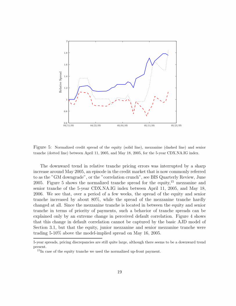
Figure 5: Normalized credit spread of the equity (solid line), mezzanine (dashed line) and senior
tranche (dotted line) between April 11, 2005, and May 18, 2005, for the 5-year CDX.NA.IG index.
The downward trend in relative tranche pricing errors was interrupted by a sharpincrease around May 2005, an episode in the credit market that is now commonly referredto as the ”GM downgrade”, or the ”correlation crunch”, see BIS Quarterly Review, June2005. Figure 5 shows the normalized tranche spread for the equity,15 mezzanine andsenior tranche of the 5-year CDX.NA.IG index between April 11, 2005, and May 18,2006. We see that, over a period of a few weeks, the spread of the equity and seniortranche increased by about 80%, while the spread of the mezzanine tranche hardlychanged at all. Since the mezzanine tranche is located in between the equity and seniortranche in terms of priority of payments, such a behavior of tranche spreads can beexplained only by an extreme change in perceived default correlation. Figure 4 showsthat this change in default correlation cannot be captured by the basic AJD model ofSection 3.1, but that the equity, junior mezzanine and senior mezzanine tranche weretrading 5-10% above the model-implied spread on May 16, 2005.
5-year spreads, pricing discrepancies are still quite large, although there seems to be a downward trendpresent.
15In case of the equity tranche we used the normalized up-front payment.
19
5.2 Parameter Stability over Time
Table 3 reports the fitted model parameters σY , κQθQ
Avg + lQµQ, and ω1 at a monthlyfrequency between September 2004 and November 2006.16 The first column shows apronounced downward trend in the volatility of default intensities, and therefore also ofCDS spread volatilities, since both quantities are closely related. The second columnindicates that optimism about the future credit market environment increased betweenSeptember 2004 and November 2006. The last column, which shows the ratio of thesystematic to total jump intensity, indicates that perceived systematic jump risk declinedrelative to firm-specific jump risk. In summary, the parameter time series in Table 3 showa significant reduction in perceived market-wide credit risk between September 2004 andNovember 2006. We also see that the risk-neutral default intensity parameter vector ΘQ
t
is relatively stable over time, especially for periods during which tranche spreads did notchange much, which is important for the model’s applicability to hedging. See Eckner(2009) for a discussion of hedging tranches against various risk factors in the creditmarket, when using the basic AJD framework of Section 3.1.
16The time series of the other model parameters are qualitatively similar and available upon request.See Eckner (2009) for a discussion and interpretation of these parameters.
Table 3: Time series of fitted model parameters at a monthly frequency between September 2004
and November 2006. σY is the volatility of the systematic risk factor, κQ the mean reversion speed of
systematic and idiosyncratic risk factors, θQ
Avg the average mean reversion level of default intensities,
lQ the jump intensity and µQ the average expected jump size of default intensities, and ω1 the fraction
of jumps that are systematic.
21
6 Joint Model for λP and λQ
This section describes a joint model for physical and risk-neutral default intensities,which allows one to quantify the sizes of various types of risk premia in the creditmarket. We start with a couple of remarks about empirical features that such a jointmodel should be able to capture.
In general, there are two types of default intensities that are of interest for a givencompany, namely its physical (or real-world) default intensity (that under P is denotedby λP
i ) and its risk-neutral default intensity (that under Q is denoted by λQi ) . The
quantity
λQit
λPit
− 1
is commonly referred to as the jump-to-default (JTD) risk premium for company i attime t, and can be seen as instantaneous compensation to investors for being exposedto the risk of instantaneous default of company i. Under the conditional diversificationhypothesis (see Jarrow, Lando, and Yu (2005)), the jump-to-default risk premium isequal to zero, since JTD risk can be diversified away. However, empirical studies havefound the average value of λQ
it/λPit−1 to be somewhere in the range between 1.5 and 4 for
corporate bonds and credit-default-swaps of BBB rated US issuers, although this valuecan fluctuate strongly over time. See for example Berndt, Douglas, Duffie, Ferguson,and Schranz (2005), Amato and Remolona (2005) and Saita (2006). Amato (2005) findsthe JTD risk premium to be inversely related to credit ratings, and to be as high as 625for AAA and as low as 2.2 for BB-rated debt. These findings indicate that the liquiduniverse of credit risky securities is probably not large enough to diversify away short-term default risk and that investors therefore demand instantaneous compensation aboveand beyond compensation for instantaneous expected losses when holding a portfolio ofcorporate credits. In addition, borrowing constraints are likely to be at least partiallyresponsible for the dramatic variation of the JTD risk premium across rating categories.For example, an investor subject to borrowing constraints might be able to reach acertain target expected return only by investing in high-yielding assets, but not bytaking a leveraged position in lower-yielding assets.17
A second type of risk premia that is deemed to be important in the credit marketis compensation for mark-to-market risk, which is the uncertainty regarding the futureevolution of risk factors in general, and default intensities in particular. See for exampleBerndt, Douglas, Duffie, Ferguson, and Schranz (2005) and Saita (2006).
17A similar explanation has been offered for the historical risk-adjusted outperformance of low-betaover high-beta stocks. See Black, Jensen, and Scholes (1972) and Black (1993).
22
6.1 Joint Model Specification
This section makes precise the joint model for physical and risk-neutral default intensi-ties. We again use an affine two-factor model of the form
λPit = bP
itXit+ aPitYt,
λQit = Xit+ aQ
itYt,(23)
for 1 ≤ i ≤ m, where Xi and Y are independent basic AJDs under P and under Q.We use time-varying model parameters ΘQ
t , but for notational simplicity suppress thistime-dependence in most equations.18 The dynamics of Xi are given by
dXit = κPi
(θP
i − Xit
)dt + σi
√Xit dB
P,(i)t + dJ
P,(i)t
dXit = κQi
(θQ
i − Xit
)dt + σi
√Xit dB
Q,(i)t + dJ
Q,(i)t
(24)
for 1 ≤ i ≤ m. Under P, BP,(i) are independent Brownian motions and JP,(i) independentcompound Poisson processes. Under Q, BQ,(i) are independent Brownian motions andJQ,(i) independent compound Poisson processes.
Similarly, the dynamics of Y are given by
dYt = κPY
(θP
Y − Yt
)dt + σY
√Yt dB
P,(Y )t + dJ
P,(Y )t ,
dYt = κQY
(θQ
Y − Yt
)dt + σY
√Yt dB
Q,(Y )t + dJ
Q,(Y )t .
(25)
Under P, BP,(Y ) is a Brownian motion and JP,(Y ) an independent compound Poissonprocess. Under Q, BQ,(Y ) is a Brownian motion and JQ,(Y ) an independent compoundPoisson process.
To simplify notation, let
APt = (aP
it)1≤i≤m AP = (APt )t≥0
BPt = (bP
it)1≤i≤m BP = (BPt )t≥0
AQt = (aQ
it)1≤i≤m AQ = (AQt )t≥0
Xt = (Xit)1≤i≤m X = (Xt)t≥0
ΛPt = (λP
it)1≤i≤m ΛP = (ΛPt )t≥0
ΛQt = (λQ
it)1≤i≤m ΛQ = (ΛQt )t≥0,
and
Y = (Yt)t≥0,ΘP
t = (κPY,t, θ
PY,t, σY,t, l
PY,t, µ
PY,t, (κ
Pi,t, θ
Pi,t, l
Pi,t, µ
Pi,t)1≤i≤m)
ΘP = (ΘPt )t≥0
ΘQt = (κQ
Y,t, θQY,t, σY,t, l
QY,t, µ
QY,t, (κ
Qi,t, θ
Qi,t, l
Qi,t, µ
Qi,t)1≤i≤m)
ΘQ = (ΘQt )t≥0,
18We briefly examined a model with time-fixed factor loadings in (23), but were unable to achievean acceptable fit since the ratios λQ
it/λPit often vary dramatically over time. See also Section 7.1.
23
and
CDSt = (ccdsi,t,M)1≤i≤m,M∈5,7,10 CDS = (CDSt)t≥0
TRt = (ctrj,t,M)1≤i≤m,M∈5,7,10 TR = (TRt)t≥0
IDXt = (cidxt,M)M∈5,7,10 IDX = (IDXt)t≥0,
where ΛP is the output of the model for physical default intensities estimated by Duffie,Saita, and Wang (2007) and Duffie, Eckner, Horel, and Saita (2009). Their model wasfitted to a 25-year US corporate default history of 2,793 companies. (See Appendix Afor details.) By taking the output of their model as given, we reduce the efficiency ofour parameter estimation procedure compared to full maximum likelihood estimation,but avoid the computational complexity that a joint estimation would require.
We must conduct inference only about Θ ≡(AP, BP, AQ, ΘP, ΘQ
)and Y, since X
is then determined implicitly by ΛP, AP, BP and Y via (23). In the following, wetherefore write Xit=Xit
(aP
it, bPit, Yt, λ
Pit
)to emphasize that Xit is determined by the data
and parameters in parentheses. For a fixed set of parameters Θ, using Bayes’ rule andthe Markov property for Xi and Y, we can write the likelihood function LΘ of the dataas
LΘ
(Y, ΛP, CDS, TR, IDX
)(26)
∝ pΘ (Y) pΘ
(ΛP, CDS, TR , IDX |Y
)
= pΘ (Y) pΘ
(ΛP |Y
)pΘ (CDS, TR, IDX |Y)
= pΘ (Y0) ×T∏
t=1
pbAJD
(Yt | Yt−1, Θ
Pt−1
)
×T∏
t=1
m∏
i=1
pbAJD
(Xit
(aP
it, bPit, Yt, λ
Pit
)|Xi,t−1
(aP
i,t−1, bPi,t−1, Yt−1, λ
Pi,t−1
), ΘP
t−1
)
×T∏
t=0
pΘ (CDSt, TRt, IDXt |Xt, Yt) ,
where pbAJD denotes the transition density of a basic AJD.For the parameter estimation, we again impose the constraints (7)-(12) on the risk-
neutral parameters, and in addition impose for each i and t,
κPi,tθ
Pit = κQ
i,tθQit
κPY,tθ
PY,t = κQ
Y,tθQY,t
aPit = ω3,tλ
Pit.
(27)
The first two conditions in (27) correspond to a completely affine specification for themarket-price of diffusive risk, and ensure that Q is indeed an equivalent martingalemeasure for P, see Appendix B for details. The last condition in (27) is used to arrive at
24
a parsimonious model. A singular value decomposition of the sample covariance matrixof (∆λP
it : 1 ≤ i ≤ m) gave a Spearman rank correlation of 0.91 between (i) the entriesof the first eigenvector and (ii) average default intensities Avgt(λ
Pit), so that taking aP
i
proportional to λPi is not overly restrictive.
Full maximum likelihood inference of the model parameters via
Θ = arg supΘ
LΘ
(Y, ΛP, CDS, TR, IDX
),
for example using MCMC methods that treat X and Y as latent variables, would bedesirable, but is computationally extremely burdensome. In addition, stale prices andmarket-microstructure noise in the CDS data would make the inference procedure proneto outliers. We therefore settled for a slightly less efficient estimation procedure ofthe model parameters, a mixture between maximum likelihood estimation and robustmethod of moments, which is computationally more tractable and gives robust parameterestimates. Before we turn to the actual fitting procedure, we need the following tworesults:
Proposition 1 Let⟨λP
i , λPj
⟩(t) denote the continuous part of the quadratic covariation
between λPi and λP
j in the time interval [0, t].19 Then
(i)⟨λP
i , λPj
⟩(t) =
∫ t
0aP
isaPjsσ
2Y,sYsds.
(ii) A consistent (for ∆t → 0) and model-free estimate of⟨λP
i , λPj
⟩(t) is given by
⟨λP
i , λPj
⟩(t) =
1
2
⟨λP
i + λPj
⟩(t) −
⟨λP
i
⟩(t) −
⟨λP
i
⟩(t)
,
where for a stochastic process X that is observed at times 0, ∆t, 2∆t, . . ., n∆t =t,
〈X〉 (t) =n−1∑
i=1
|∆Xi∆t|∣∣∆X(i+1)∆t
∣∣
denotes its realized power variation.
The first property follows directly from the definition of physical default intensitiesvia (23), (24) and (25), while the second property follows from the results in Barndorff-Nielsen and Shephard (2004).
19The derivative of this process can be thought of as the instantaneous Brownian covariance betweenλP
i and λPj .
25
Based on this corollary, we use
CovP
cont
(λP
it, λPjt
)≡⟨λP
i , λPj
⟩(t) −
⟨λP
i , λPj
⟩(t − 180)
180
as a rolling estimate of the continuous covariance between λPi and λP
j at time t, wheretime is measured in days.
The fitting procedure is follows:
Algorithm 2
1. Fit X, Y, and ΘQ (including σY,t : 0 ≤ t ≤ T) to the monthly times series of 5, 7and 10-year CDS, credit index, and tranche spreads, again using the robust version(21) of tranche pricing errors.20
2. The relation aPit = ω3,tλ
Pit in (27) implies that
CovPcont
(λP
it, λPjt
)= aP
itaPjtCovP
cont(Yt, Yt)
= ω23,tλ
Pitλ
Pjtσ
2Y,tYt.
Hence for S = (i, j) : 1 ≤ i, j ≤ m, i 6= j,
median(i,j)∈SCovPcont
(λP
it, λPjt
)= ω2
3,tσ2Y,tYt · median(i,j)∈S
(λP
itλPjt
),
so that a robust estimate of ω3,t is
ω3,t =
√√√√median(i,j)∈SCovP
cont
(λP
it, λPjt
)
σ2Y,tYt · median(i,j)∈S
(λP
itλPjt
) .
3. Calculate the factor loadings aPit and bP
it of physical default intensities on the com-mon and firm-specific factors, respectively, via
aPit = ω3,tλ
Pit
bPit =
λPit − aP
itYt
Xit
=λP
it (1 − ω3,tYt)
Xit
·
20Excluding May 2005, the mean and standard deviation of the standardized residuals εY,t+1 =∆Yt+1/(σY,t
√Yt∆t) are equal to -0.14 and 1.06, respectively. A Kolmogorov-Smirnov test against a
standard normal distribution gave a p-value of 0.83. Hence, the volatility parameter time series σY,t isfairly consistent with the time-series behavior of Y, even though this property was not enforced in theestimation.
26
4. Given X, Y, σY,t : 0 ≤ t ≤ T, and σXi,t : 1 ≤ i ≤ m, 0 ≤ t ≤ T, fit ΘP via max-imum likelihood estimation, taking into account the completely affine constraints(27). Due to the limited length of the dataset, we in addition impose the cross-sectional constraints, for all i,
κPi
= κPX
lPi = lPXµP
i = µPX ,
where κPX , lPX and µP
X are constants. For the common factor Y, we set
κPY =
ln (2)
3≈ 0.23,
so that the half-life of a systematic shock is equal to three years, which is at the up-per end of half of the typical US business cycle length, see King and Watson (1996),and therefore leads to a conservative estimate of the market price of systematic riskin (28) below. Moreover, we set
lPY = lQYµP
Y = µQY ,
which leads to a conservative estimate of risk premia associated with the systematicfactor.
Maximum likelihood estimation in Step 4 amounts to parameter inference about adiscretely-observed basic AJD. See Appendix C for details.
Remark 2 Step 4 in Algorithm 2 relies on the assumption that the parameters governingphysical default intensity dynamics do not change over time. In particular, companieshave a stationary capital structure and the mechanism by which companies default doesnot exhibit any structural breaks. A change in legislation, like the Sarbanes-Oxley Actof 2002, might cause a permanent shift in the default pattern of corporations, everythingelse equal, so that this assumption may be violated.
6.2 Risk Premia
After specifying the joint model of physical and risk-neutral default intensity dynamics,we are able to describe the difference between the probability measures P and Q in termsof the Radon-Nikodym derivative dQ/dP. For the framework of Section 6.1, AppendixB provides an explicit formula for dQ/dP and lists technical conditions under which Qis indeed an equivalent martingale measure for P. A convenient way to ”summarize” theRadon-Nikodym derivative dQ/dP is in terms of risk premia, namely:
27
1.) The market price of diffusive risk (systematic and firm-specific)
2.) The pure jump-to-default risk premium
3.) The correlation risk premium
4.) The market price of jump arrival risk
5.) The market price of jump size risk
Theorem 5 in Appendix B shows that the Radon-Nikodym derivative dQ/dP canbe written in terms of the above risk premia, whose definitions are made precise in theremainder of this section. Hence, there is no information ”lost” by directly using theserisk premia to evaluate investors’ risk preferences in the credit markets.
6.2.1 Market Price of (Diffusive) Risk
The market price of risk measures the compensation that investors receive for beingexposed to the risk that the realized value of a certain risk factor will turn out to be lessfavorable than expected. Let Z be a basic AJD with
dZt = κP(θP − Zt
)dt + σ
√Zt dBP
t + dJPt
dZt = κQ(θQ − Zt
)dt + σ
√Zt dBQ
t + dJQt .
Under P, BP,(Y ) is a Brownian motion and JP,(Y ) an independent compound Poissonprocess with jump intensity lP,(Z) and exponentially distributed jumps with mean µP,(Z).Under Q, BQ,(Y ) is a Brownian motion and JQ,(Y ) an independent compound Poissonprocess with jump intensity lQ,(Z) and exponentially distributed jumps with mean µQ,(Z).We call
ηMPR(Diff) (Zt) =κQθQ − κPθP
σ√
Zt
+κQ − κP
σ
√Zt
the market price of diffusive risk for Z. The constraint κQθQ = κPθP of the completelyaffine risk premia specification implies that
ηMPR(Diff) (Zt) =κQ − κP
σ
√Zt.
Hence, for the joint model of default intensities in Section 6.1, the market price ofdiffusive risk is
ηMPR(Diff) (Xit) =κQ − κP
σi
√Xit =
κQ − κP
σ
√Xit
aQi
28
for the firm-specific risk factors and
ηMPR(Diff) (Yt) =κQ − κP
σ
√Yt. (28)
for the systematic risk factor.
6.2.2 Jump-to-Default and Correlation Risk Premium
In the framework of Section 6.1, risk-neutral default intensities can be rewritten as
λQit = Xit + aQ
itYt =
=bPit
bPit
Xit +aP
it
bPit
Yt +
(aQ
it −aP
it
bPit
)Yt =
=1
bPit
λPit +
(aQ
it −aP
it
bPit
)Yt.
We call
ηpJTD(λQ
it
)=
1
bPit
− 1
the pure jump-to-default (pJTD) risk premium and
ηCor(λQ
it
)=
(aQ
it −aP
it
bPit
)(29)
the correlation risk premium of company i at time t. Under this convention, risk-neutraldefault intensities can be written as
λQit = λP
it + ηpJTD(λQ
it
)λP
it + ηCor(λQ
it
)Yt, (30)
reflecting instantaneous compensation for expected losses, pure jump-to-default risk andcorrelation risk.
Remark 3 Our definition of the JTD risk premium is slightly different than the onecommonly used in the literature, which is λQ
it/λPit − 1 (see for example Driessen (2005)
Berndt, Douglas, Duffie, Ferguson, and Schranz (2005), Amato (2005) and Saita (2006)),since a multivariate model of credit risk allows one to further break down λQ
it/λPit − 1
into compensation for pure JTD risk and correlation risk. See also Collin-Dufresne,Goldstein, and Helwege (2003) for a non-doubly-stochastic framework where λQ
it/λPit − 1
can be decomposed into compensation for pure JTD risk (called timing risk in the paper)and contagion risk.
29
Remark 4 Definition (29) of the correlation risk premium is warranted, since in adoubly-stochastic setting, default time correlation is entirely attributable to correlationacross firms’ levels of future credit-worthiness, which in our case is driven by the sys-tematic factor Y . In the presence of contagion, influence would also be able to ”flow” inthe opposite direction, in the sense that the default of a particular firm can impact thejoint future credit-worthiness of surviving companies above and beyond economic con-ditions. In this case, the correlation risk premium would consist of compensation for (i)correlation of future credit-worthiness due to joint dependence on economic conditionsand (ii) default contagion.
6.2.3 Market Price of Jump Arrival Risk
The market price of jump arrival risk is defined as
ηMPR(JA) (Xit) =lQilPXi
for the idiosyncratic risk factors. Recall that due to the limited length of our dataset,we assumed in Section 6.1 that ηMPR(JA) (Yt) is equal to zero, so that the market price ofjump arrival risk for the common factor is subsumed into the correlation risk premium.
6.2.4 Market Price of Jump Size Risk
The market price of jump size risk is defined as
ηMPR(JS) (Xit) =µQ
i
µPXi
for the idiosyncratic risk factors. Recall that due to the limited length of our dataset,we assumed in Section 6.1 that ηMPR(JS) (Yt) is equal to zero, so that the market priceof jump size risk for the common factor is subsumed into the correlation risk premium.
7 Results – Risk Premia
This sections presents the fit of the joint model for physical and risk-neutral defaultintensities. It also describes a decomposition of credit tranche spreads into compensationfor expected losses and various types of risk premia.
7.1 Case Study – Alcoa Inc.
We start with a short case study to illustrate the differences between physical andrisk-neutral default intensities. For this purpose, we picked Alcoa Inc. (ticker symbol
30
0.2
0.5
1
2
5
10
20
50
100
Sep04 Feb05 Jun05 Oct05 Feb06 Jun06 Oct06
Basi
sPoin
ts
Figure 6: Evolution of default risk for Alcoa Inc. at a monthly frequency: 5-year CDS spread divided
by 0.6 (solid line), risk-neutral default intensity λQit (dotted line), and physical default intensity λP
it
(dashed line). Risk-neutral default intensities are from the fitted basic AJD model, while physical
default intensities are from the Cox proportional hazards model estimated by Duffie, Saita and Wang
(2007), and Duffie, Eckner, Horel and Saita (2006).
AA), which as of July 2007 had a market capitalization of $36bn and had maintaineda credit rating of ’A’ between September 2004 and November 2006. The historical one-year default probability for this rating category is 0.08% according to Moody’s InvestorService, ”Historical Default Rates of Corporate Bond Issuers, 1920-1999”.
Figure 6 shows the fitted physical and risk-neutral default intensity for Alcoa Inc.between September 2004 and November 2006, together with the 5-year CDS spreaddivided by 0.6, which for low-risk issuers is a rough estimate of the average risk-neutralyearly default rate over the next five years. As expected, physical and risk-neutraldefault intensities are highly correlated, having a sample correlation of 0.62, while thesample correlation of monthly changes in intensities is 0.48. We also see that the risk-neutral default intensity has been consistently higher than the physical default intensity,indicating that jump-to-default and/or correlation risk is priced in the decomposition(30).21 We also see that the ratio of the risk-neutral to physical default intensity λQ
i /λPi
21For about 90% of the companies in our dataset, this pattern holds at each single point in time
31
can vary considerably over time. For example, between May 2005 and November 2006this ratio dropped from a value around 20 to a value around 5, which indicates thatin our framework it would be difficult to fit a model with constant factor loadings in(23) to the time series of physical and risk-neutral default intensities.22 Finally, we seethat the average risk-neutral yearly default rate over the next five years is consistentlyhigher than the risk-neutral default intensity λQ
i , reflecting the typical upward-slopingterm-structure of default rates for investment-grade rated issuers.
7.2 Fitted Parameters
The fitted risk-neutral model parameters ΘQ from Step 1 in Algorithm 2 are similar tothose in Section 5, and therefore not reported here. Idiosyncratic credit risk shocks arehighly mean reverting under the physical probability measure, with κP
X = 1.34. Moreover,idiosyncratic jumps are more frequent (lPX = 0.992) and smaller (µP
X = 12.5 basis points)under the physical probability measure than under the risk-neutral probability measure.
Figure 7 shows the time series of the median ratios aPit/a
Qit and bP
it/bQit, where the
median is taken at each point in time over the set of CDX.NA.IG members on that day.We see that bP
it/bQit is consistently less than one between September 2004 and November
2006, indicating that for the median firm, the pure jump-to-default risk premium ispositive in the decomposition (30) of risk-neutral default intensities. Most of the timethe median ratio aP
it/aQit is smaller than the median ratio bP
it/bQit, so that the median
correlation risk premium (29) is positive. Only around May 2005 did the correlationrisk premium turn significantly negative.
7.3 Tranche Spread Decomposition
The joint model for physical and risk-neutral default intensities allows one to decom-pose credit index and tranche spreads into compensation for expected losses and therisk premia described in Section 6.2. To this end, we combine the market price of diffu-sive, jump-arrival, and jump size risk (ηMPR(Diff) (Xit), ηMPR(JA) (Xit) and ηMPR(JS) (Xit),respectively) for the idiosyncratic factors Xi and simply call
the market price of firm-specific risk. The market price of diffusive risk and the marketprice of jump risk are highly collinear, since risk-neutral drifts and jump parameters arehighly collinear, and are therefore poorly identified separately.
between September 2004 and November 2006. For the remaining 10% of the companies, the patternstill holds most of the time.
22On May 2, 2005, and November 1, 2006, the share price of Alcoa Inc. was 29.19 and 28.33,distance-to-default 5.93 and 5.59, and the five-year CDS spread 39 bps and 17 bps, respectively.
32
0
0.05
0.1
0.15
0.2
0.25
0.3
0.35
0.4
0.45
0.5
Sep04 Feb05 Jun05 Oct05 Feb06 Jun06 Oct06
Ratio
Figure 7: Median ratio aPit/aQ
it (solid line) and bPit/bQ
it (dashed line), where the median is taken at each
point in time over the set of current CDX.NA.IG members.
Hence, we are left with four different risk premia and the following intuitive inter-pretations:
Market Price of Systematic Risk: Measures the amount of expected return thatinvestors are willing to give up in order to guarantee that the economy developsas expected.
Market Price of Firm-Specific Risk: Given the market-wide performance, this mea-sures the amount of expected return that investors are willing to give up in orderto guarantee that a certain company performs in-line with the economy.
Correlation Risk Premium: Measures the amount of expected return that investorsare willing to give up to guarantee that the future credit-worthiness of a cer-tain company is uncorrelated (as opposed to positively correlated) with the futuremarket-wide credit environment.
Pure Jump-to-Default Risk Premium: Measures investors’ compensation for theuncertainty associated with the timing of default events, given both market-wide
33
and firm-specific risk factors that determine default probabilities.23
The decomposition of tranche spreads into compensation for different sources of riskis now obtained as follows:
Expected losses: Set the risk premia ηMPR (Xit), ηpJTD (Xit), ηCor (Xit) for 1 ≤ i ≤ m,and ηMPR(Diff) (Yt) equal to zero. Recalculate credit index and tranche spreads.The ratio of the new spread to the original spread represents the fraction of thespread that is compensation for expected losses.
Risk Premia: The remaining fraction of credit spreads is distributed among (i) themarket price of systematic risk, (ii) the market price of idiosyncratic risk (iii)the pure jump-to-default risk premium and (iv) the correlation risk premium.The proration is done by setting these risk premia equal to zero, one at a time,recalculating index and tranche spreads, and setting the spread contribution ofeach risk premium proportional to the resulting reduction in index and tranchespreads.24
Figure 1 in the introduction shows the resulting decomposition of credit index andtranche spreads for the 5-year CDX index on November 1, 2006, which is the most re-cent available date in our dataset. As expected, the equity tranche up-front paymentmainly represents compensation for expected losses due to defaults, compensation forthe risk of firm-specific credit deterioration, and compensation for the uncertainty asso-ciated with the timing of defaults. As one moves up the capital structure, the fraction oftranche spreads that is compensation for the risk of a market-wide credit deteriorationand compensation for correlation risk increases, and in case of the senior tranche ac-counts for more than 95% of the total spread. As a consequence, senior mezzanine andsenior tranche spreads are likely to be much more sensitive to changes in investors’ riskpreferences than to changes in expected losses. This view has been expressed by manyresearchers and practitioners (see Tavakoli (2003)), but to the best of our knowledge hasnot previously been quantified.
In a manner analogous to the tranche spread decomposition above, one can obtaina decomposition of risk-neutral expected portfolio losses into compensation for differ-ent sources of risks, and attribute these components to individual tranches. For thetime period from September 2004 to November 2006, Table 4 shows sample averagesof the fractions of risk-neutral expected portfolio losses that correspond to individual
23Compensation for correlation risk premium and the pure jump-to-default risk would not be sepa-rately identifiable in a univariate setting.
24Alternatively, one can sequentially add the risk premia. We found the resulting decomposition oftranche spreads to be almost identical to the currently used decomposition. However, it is not clear inwhich order the individual risk premia should be added.
34
source-of-risk/tranche pairs. The last column and row show the total fraction of risk-neutral expected portfolio losses that can be attributed the individual sources of risksand tranches, respectively. Note that the total sum of the fractions is slightly less thanone, since the super senior (30 - 100%) tranche is not included in Table 4 due to lack ofavailable data. We see that by far the largest component of risk-neutral expected port-folio losses is compensation to the equity tranche for idiosyncratic risk (28%), followedby compensation to the equity tranche for pure JTD risk (22.7%), followed by com-pensation to the equity tranche for actual expected losses (19.7%), and then followedby compensation to the junior mezzanine tranche for systematic risk (4.2%). We alsosee that compensation to senior tranches is only a small fraction (<2%) of risk-neutralexpected portfolio losses, and that this fraction is mostly compensation for systematicand correlation risk.
Table 4: Attribution of risk-neutral expected portfolio losses to tranches and sources of risk. En-
try (i, j) is the fraction of risk-neutral expected portfolio losses that is compensation of risk source i
to tranche j. Data are sample averages for the 5-year CDX North-America Investment-Grade index
between September 2004 and November 2006. Sample standard deviations are given parenthetically.
Remark 5 In an analogous manner, such a decomposition can be achieved for othercredit derivatives, like CDS contracts or first-to-default baskets.
Remark 6 Since the number of defaults in our sample period (September 2004 toNovember 2006) was unusually low by historical standards, the contribution of expectedlosses to tranches spreads is likely underestimated in Figure 1 and Table 4. It would bedesirable to repeat our analysis for a period that covers a full economic cycle, as soonas these data become available.
35
7.4 Tranche Vs. CDS Risk Characteristics
Coval, Jurek, and Stafford (2007) argue that certain structured finance instruments,such as a senior CDO tranche, offer far less compensation than alternative pay-off pro-files, such as a short position in a 50% out-of-the-money put option on the S&P500index. They argue that this mispricing is due to the tendency of rating agencies topay attention only to expected losses when assigning ratings, but not to in what stateof the economy these losses are going to occur. Under this presumption, issuing CDOtranches emerges as a mechanism for exploiting investors who solely rely on ratings forinvestment decisions.
To examine this point further, Table 5 provides the credit spread decomposition onNovember 1, 2006, for (i) the senior mezzanine tranche (10%-15%) of the 5-year CDXNorth-America Investment-Grade Index and (ii) a 5-year CDS contract for Wal-MartStores, Inc., which had a AA credit rating on this particular date. With a spread of 7.0and 7.7 basis points, respectively, the implied risk-neutral probability of a loss to theseller of protection is extremely low for these two credit derivatives. The first row in Table5 shows that the fraction of the credit spread that is compensation for expected losses,is about twice as high for the CDS contract compared to the CDX tranche contract.25
In other words, for a given amount of expected losses, a seller of protection for a seniormezzanine CDX tranche can get an expected return that is roughly twice as high as thoseof a seller of protection for a CDS contract with similar pay-off profile. Hence, we do notfind evidence that investors are fully oblivious about the differences in the risks betweenstructured and single-name credit products. Further research in this area is required, toasses whether investors are at least partially oblivious about these differences, as arguedby Coval, Jurek, and Stafford (2007).
Table 5: Fraction of spread that is compensation for different sources of risk. Data are for November
1, 2006, for (i) the senior mezzanine tranche (10% - 15%) of the 5-year CDX North-America Investment-
Grade Index and (ii) the 5-year CDS spread of Wal-Mart Stores, Inc.
25A similar relationship seems to hold for other highly rated issuers in the CDX portfolio. Of course,these results depend on a range of modeling assumption.
36
8 Conclusion
The emphasis of this paper has been two-fold. First, we conducted an empirical analysisof an extensive dataset of CDS, credit index, and credit tranche spreads between Septem-ber 2004 and November 2006. To these data, we fitted an intensity-based model for thejoint behavior of corporate default times, along the lines of Duffie and Garleanu (2001),Mortensen (2006), and Eckner (2009). We found that the largest 5-year CDX.NA.IGtranche pricing errors occurred shortly after the introduction of the CDX index andtranche contracts, but that these discrepancies largely disappeared within a couple ofmonths, either reflecting an evolution towards a more efficient market for structuredcredit derivatives, or more homogeneity in the models applied in industry practice.However, this downward trend in tranche pricing errors was interrupted by a sharp in-crease around May 2005, an episode in the credit market that is now commonly referredto as the ”GM downgrade”, or the ”correlation crunch”.
Second, we introduced a joint model for physical and risk-neutral default intensities,which we fitted to the time series of credit-default-swap, credit index, and credit tranchespreads between September 2004 and November 2006, as well as to the physical defaultintensity output from Duffie, Saita, and Wang (2007), and Duffie, Eckner, Horel, andSaita (2009). We presented a decomposition of risk-neutral expected portfolio lossesinto compensation for different sources of risks, and attributed these components toindividual tranches. For our sample period we found that investors in the CDX first-losstranche on average bear about 93.3% of the expected losses on the underlying portfolio ofcorporate debt, and receive about 77.0% of the total compensation for bearing portfoliolosses. On the other hand, investors in the senior tranche, on average, bear about0.2% of expected default losses on the underlying portfolio, and receive about 2% of thetotal compensation. In terms of the ratio, on average, of compensation rate per unit ofexpected loss, the first-loss piece carries a risk premium of 3.9, whereas the most seniortranches offer a risk premium of about 50. This extreme difference in risk premia isnatural given that the most senior tranches bear losses only when there is a significant”meltdown” in corporate performance.
Although Coval, Jurek, and Stafford (2007) argued that investors in senior CDOtranches underprice systematic risks by solely relying on credit ratings for the purposeof making investment decisions, we found that investors are reasonably aware about thedifferences in the risks between structured and single-name credit products. However, inour framework we cannot preclude that investors are at least partially oblivious aboutthese differences, and further research in this area would be desirable.
Finally, we broke down the compensation for bearing default risk into several com-ponents, namely compensation for actual expected losses, systematic risk, firm-specificrisk, correlation risk, and pure jump-to-default (JTD) risk. We showed that varioustranches have different rates of compensation per unit of expected loss because theycarry these various types of risks in different proportions to each other. For our sample
37
period, the equity tranche is allocated 81.7% of the total compensation for firm-specificrisk in the underlying portfolio of debt, but carries only 32.0% of the total compensationfor systematic risk. The senior tranche, on the other hand, is allocated only 0.2% ofthe total compensation for firm-specific risk, but carries a relatively large fraction, 9.9%,of the total compensation for systematic risk. We hope that this breakdown will provevaluable to investors in single-name and structured credit products, who would like tobetter understand the types of risks to which they are exposed to, and to quantify theextent to which they are being compensated for these risks.
38
Appendices
A Cox Proportional Hazards Model for λP
Using 25 years of US corporate default history on 2,793 companies, Duffie, Saita, andWang (2007) and Duffie, Eckner, Horel, and Saita (2009) estimated a Cox proportionalhazards model for physical default intensities. The default intensity of firm i at time tis given by
λPit = eβ·Wit,
where β is a parameter vector, and Wit a vector of firm-specific and macroeconomiccovariates. The covariates are (i) distance-to-default, which is a volatility-adjusted mea-sure of leverage, (ii) the firm’s trailing 1-year stock return, (iii) the 3-month Treasurybill rate, and (iv) the trailing 1-year return on the S&P 500 index. See Duffie, Saita,and Wang (2007) and Duffie, Eckner, Horel, and Saita (2009) for a detailed descriptionof the covariates and the maximum likelihood estimate of the parameter vector β. Notsurprisingly, distance-to-default is the most influential covariate for determining defaultintensities, but the other covariates are statistically and economically significant as well.
B Equivalent Martingale Measure Conditions
This section provides technical conditions for the dynamics of λP under P, and λQ underQ, that ensure that Q is indeed an equivalent martingale measure for P. Standardreferences on equivalent martingale measures and risk-neutral pricing include Harrisonand Kreps (1979) for a discrete time setting, Harrison and Pliska (1981) for the Brownianmotion setting, Bremaud (1981) for point processes, Dai and Singleton (2000) for thecompletely affine market price of risk specification, and Cheridito, Filipovic, and Kimmel(2005) and Cheridito, Filipovic, and Yor (2005) for more general affine processes andchanges of measure.
In the framework of Section 6, physical and risk-neutral default intensities are givenby
λQit = Xit + aiYt
λPit = λQ
it/(1 + ηJTDit ),
for 1 ≤ i ≤ m, where the jump-to-default risk premium ηJTDi can represent compensation
for pure JTD risk and for correlation risk, see decomposition (30). To simplify notation,let Z = (Z1, . . . , Zm+1) = (X1, . . .Xm, Y ) denote the vector of stochastic processes
39
driving default intensities. The dynamics of Zj are given by
dZjt = (κP,(Zj)0 + κ
P,(Zj)1 Zjt) dt + σZj
√Zjt dB
P,(Zj)t + dJ
P,(Zj)t
dZjt = (κQ,(Zj)0 + κ
Q,(Zj)1 Zjt) dt + σZj
√Zjt dB
Q,(Zj)t + dJ
Q,(Zj)t .
(31)
Under P, BP,(Zj) are independent Brownian motions, and JP,(Zj) are independent com-pound Poisson processes with jump intensities lP,(Zj) and exponentially distributed jumpswith mean µP,(Zj). Under Q, BQ,(Zj) are independent Brownian motions, and JQ,(Zj) areindependent compound Poisson processes with jump intensities lQ,(Zj) and exponentiallydistributed jumps with mean µQ,(Zj). The completely affine risk premia specificationimposes the parameter constraints, for each j,
κP,(Zj)0 = κ
Q,(Zj)0 .
We next show that the density (Radon-Nikodym derivative)
Λt = E
(dQ
dP| Ft
)
can be written as a product of factors representing (i) changes in the drift of the m + 1Brownian motions, (ii) changes in the m+1 jump intensities and jump size distributions,and (iii) scaling of the m intensities λP
i by one plus the jump-to-default risk premium.Specifically,
Λt =
(m+1∏
j=1
Λ(1)jt
)(m+1∏
j=1
Λ(2)jt
)(m∏
i=1
Λ(3)it
)(32)
=
(dQ
dP
)
t
(dQ
dQ
)
t
(dQ
dQ
)
t
.
The first two factors in (32) represent the change in dynamics of Zj under P to Zj underQ, while the last term reflects the change from λP
i under Q to λQi under Q. The remainder
of this Appendix provides technical conditions for (32) to define an arbitrage-free pricingmeasure Q equivalent to P.
The following proposition governs the drift change of the stochastic processes Zj.See Dai and Singleton (2000) for details.
Proposition 2 Fix a time horizon T > 0. Assume that, for each j,
κP,(Zj)0 = κ
Q,(Zj)0 .
Define the market price of (diffusive) risk for Zj as
ηMPR(Diff) (Zjt) =κ
Q,(Zj)1 − κ
P,(Zj)1
σZj
√Zjt.
40
Then QT , defined by
E
(dQT
dP| Ft
)=
m+1∏
j=1
exp
(−∫ t
0
ηMPR(Diff) (Zjs) dBP,(Zj)s − 1
2
∫ t
0
[ηMPR(Diff) (Zjs)
]2ds
),
is a probability measure equivalent to P. Moreover, under QT the dynamics of Zj for
1 ≤ j ≤ m+1 are the same as under P except that the mean-reversion coefficient κP,(Zj)1
in (31) is replaced by κQ,(Zj)1 .
The following proposition governs the change in the jump intensity and jump sizedistribution of the stochastic processes Z1, . . . , Zm+1. See Cheridito, Filipovic, and Yor(2005) for a similar formulation.
Proposition 3 Fix a time horizon T > 0. Let νPj (z, ·) and νQ
j (z, ·) denote the jump sizedistribution of Zj under P and Q, respectively. Assume that the jump intensities underP and Q are bounded away from zero and bounded above, that is
is a probability measure equivalent to QT . Moreover, under QT the dynamics of Zj for1 ≤ j ≤ m + 1 are the same as under QT , except that the jump intensity and jump sizedistribution are now given by lQ,(Zj) and νQ
j (z, ·), respectively.
41
Remark 7 In the case of exponentially distributed jumps and constant jump intensities
φj (z, ζ) = 1ζ≥zlQ,(Zj)
lP,(Zj)
µP,(Zj)
µQ,(Zj)exp
((1
µP,(Zj)− 1
µQ,(Zj)
)(ζ − z)
).
Hence (33) is satisfied if lP,(Zj), lQ,(Zj), µP,(Zj) and µQ,(Zj) are positive.
Propositions 2 and 3 govern the technical conditions for the change in dynamics ofZj (and hence also λP
i ) under P to the dynamics under Q. The last step is a scaling ofλP
i by one plus the jump-to-default risk premium ηJTDi . Note that the Q-dynamics of
the physical default intensity λPi and of the jump-to-default risk premium ηJTD
i are notdirectly observable from market data (as opposed to historical default data or CDS andtranche spreads). Only the Q-dynamics of the product
λPi
(1 + ηJTD
i
)= λQ
i
are observable, namely via the prices of various credit derivative contracts. Since theQ-dynamics of λP
i and ηJTDi are not separately identifiable in our framework, and we
make the following assumption.
Assumption 2 The Q-dynamics of ηJTDi for 1 ≤ i ≤ m are the same as the P-dynamics.
That is, there is no risk premium associated with the evolution of jump-to-default riskpremium over time.
We can now turn to the last step in the change of measure from P to Q. For detailssee Bremaud (1981) or Duffie (2001), Proposition F.5.
Proposition 4 Fix a time horizon T > 0. Assume that (1 + ηJTDi ) is a strictly positive
and predictable process with∫ T
0
(1 + ηJTD
it
)λP
itdt < ∞ QT − almost surely.
Further assume that the local martingales
Λ(3)it = exp
(−∫ t
0
ηJTDis λP
isds
)(1τ i≤t
(1 + ηJTD
i,τ i
)+ 1τ i>t
)
are in fact QT−martingales for 1 ≤ i ≤ m and 0 ≤ t ≤ T . Then the probability measureQT , defined by
E
(dQT
dQT
| Ft
)=
m∏
i=1
Λ(3)it
is equivalent to QT . Moreover, the dynamics of λQi ≡ λP
i ηJTDi under QT are the same as
that of Xi + aiY under QT .
42
The following theorem combines the above propositions and assumptions.
Theorem 5 Fix a time horizon T > 0. Suppose the conditions in Proposition 2, 3 and 4are satisfied and that Assumption 2 holds. Then (Λt : 0 ≤ t ≤ T ), with Λt given by (32) ,is a strictly positive Ft−martingale under P, and ΛT is the Radon-Nikodym derivativeof a probability measure QT equivalent to P.
For 0 ≤ t ≤ s ≤ T , the unique arbitrage-free price at time t for a security that paysone monetary unit at time s if τ i > s (and zero otherwise) is
Vt = EQT
(e−
∫ s
trudu1τi>s | Ft
). (34)
Equivalently,
Vt = Pte∫ t
0rudu
is a martingale on (Ω,FT , (Ft : 0 ≤ t ≤ T ) , QT ).
Proof Proposition 2 implies that QT is equivalent to P. Proposition 3 implies thatQT is equivalent to QT . Proposition 4 implies that QT is equivalent to QT . We thereforealso have that QT is equivalent to P and that ΛT > 0 almost surely under P. Since
Λt = E
(dQT
dP| Ft
)= E (ΛT | Ft) ,
it follows that Λt > 0 almost surely under P. The tower property implies that (Λt : 0 ≤ t ≤ T )is an Ft−martingale under P. Finally, the security pricing formula (34) follows form thegeneral theory of arbitrage-free pricing, see for example Section 6 in Duffie (2001).
Note that it is easy to generalize (34) to the pricing of securities with more compli-cated pay-off structures, see for example Section 6L in Duffie (2001).
C MLE of Physical Default Intensity Dynamics
This section provides details about Step 4 of Algorithm 2, which involves the estimationof the parameters governing physical default intensity dynamics.
Recall that Xit : 1 ≤ i ≤ m, 0 ≤ t ≤ T and Yt : 0 ≤ t ≤ T are outputs of the fit-ting procedure in Section 4.2. Inference about the parameters governing the P−dynamicsof Xi and Y therefore amounts to estimating the parameters of a discretely observedbasic AJD. For such a process Z with parameters η = (κ, θ, σ, l, µ), let pbAJD (. | z, η, s, t)
43
denote its transition density between times s and time t for Zs = z. Given a set ofobservations Zt1 , . . . , ZtM, the likelihood function Lη is
Lη (Zt1 , . . . , Ztk) = p (Zt1 | η)
M∏
k=2
pbAJD
(Ztk |Ztk−1
, η, tk−1, tk), (35)
where p (Zt1 | η) the initial distribution of the process. We base inference about the basicAJD parameters on the time-discretization
∆Zj,tk = Zj,tk − Zj,tk−1= κ
(θ − Ztk−1
)∆tk + σ
√Ztk−1
∆tkεtk + ∆Jtk , (36)
where ∆tk = tk − tk−1, εtk are independent standard normal random variables, and ∆Jtk
are independent random variables with distribution
P (∆Jtk ∈ [z, z + dξ)) =
exp (−l∆tk) , for z = 0(1 − exp (−l∆tk))µ exp (−µz) dξ, for z > 0
The discretization (36) assumes that at most one jump can occur in each time interval(tk−1, tk]. In simulation studies, Eraker (2001) and Eraker, Johannes, and Polson (2003)show that when using daily or monthly data and parameters values similar to ours, thediscretization bias due to using (36) is negligible.
Since X1, . . . , Xm, Y are independent, parameter inference via (35) can be conductedseparately for each process, for example, via Newton-Raphson maximization of the like-lihood function. Nevertheless, it is easy to impose joint constraints on the parametersif desired.
44
References
Altman, E. I. (1968). Financial Ratios, Discriminant Analysis, and the Prediction OfCorporate Bankruptcy. Journal of Finance 23, 589–609.
Amato, J. D. (2005). Risk aversion and risk premia in the CDS market. BIS QuarterlyReview, December 2005.
Amato, J. D. and E. M. Remolona (2005). The Pricing of Unexpected Credit Losses.BIS Working Paper No. 190.
Barndorff-Nielsen, O. E. and N. Shephard (2004). Power and Bipower Variation withStochastic Volatility and Jumps. Journal of Financial Econometrics 2, 1–37.
Berndt, A., R. Douglas, D. Duffie, M. Ferguson, and D. Schranz (2005). MeasuringDefault-Risk Premia from Default Swap Rates and EDFs. BIS Working Paper No.173.
Black, F. (1993). Beta and Return. Journal of Portfolio Management 20, 8–18.
Black, F., M. Jensen, and M. Scholes (1972). The Capital Asset Pricing Model: SomeEmpirical Tests. In ”Studies In The Theory Of Capital Markets”, Praeger Pub-lishers Inc.
Bremaud, P. (1981). Point Processes and Queues: Martingale Dynamics. SpringerSeries in Statistics, New-York.
Chen, L., P. Collin-Dufresne, and R. S. Goldstein (2006). On the Relation Betweenthe Credit Spread Puzzle and the Equity Premium Puzzle.
Cheridito, P., D. Filipovic, and R. L. Kimmel (2005). Market Price of Risk Spec-ifications for Affine Models: Theory and Evidence. Journal of Financial Eco-nomics forthcoming.
Cheridito, P., D. Filipovic, and M. Yor (2005). Equivalent and Absolutely ContinuousMeasure Changes for Jump-Diffusion Processes. Annals of Applied Probability 15,1712–1732.
Collin-Dufresne, P., R. Goldstein, and J. Helwege (2003). Is Credit Event Risk Priced?Modeling Contagion via The Updating Of Beliefs. Working Paper, Haas School,University of California, Berkeley.
Collin-Dufresne, P., R. S. Goldstein, and J. S. Martin (2001). The Determinants ofCredit Spread Changes. Journal of Finance 56, 2177–2207.
Coval, J. D., J. W. Jurek, and E. Stafford (2007). Economic Catastrophe Bonds. HBSWorking Paper Number: 07-102.
Duffie, D. (2001). Dynamic Asset Pricing Theory (Third edition). Princeton, NewJersey: Princeton University Press.
Duffie, D., A. Eckner, G. Horel, and L. Saita (2009). Frailty Correlated Default.Journal of Finance 64, 2087–2122.
Duffie, D., D. Filipovic, and W. Schachermayer (2003). Affine Processes and Applica-tions in Finance. Annals of Applied Probability 13, 984–1053.
Duffie, D. and N. Garleanu (2001). Risk and Valuation of Collateralized Debt Obli-gations. Financial Analysts Journal 57, 41–59.
Duffie, D., J. Pan, and K. Singleton (2000). Transform Analysis and Asset Pricing forAffine Jump-Diffusions. Econometrica 68, 1343–1376.
Duffie, D., L. Saita, and K. Wang (2007). Multi-Period Corporate Default Predictionwith Stochastic Covariates. Journal of Financial Economics 83, Issue 3, 635–665.
Duffie, D. and K. Singleton (1999). Modeling Term Structures Of Defaultable Bonds.Review of Financial Studies 12, 687–720.
Duffie, D. and K. Singleton (2003). Credit Risk. Princeton, New Jersey: PrincetonUniversity Press.
Eckner, A. (2009). Computational Techniques for basic Affine Models of PortfolioCredit Risk. Journal of Computational Finance 12, Issue 4, xx–xx.
Elton, E., M. Gruber, D. Agrawal, and C. Mann (2001). Explaining the Rate Spreadon Corporate Bonds. Journal of Finance 56, 247–277.
Eraker, B. (2001). MCMC Analysis of Diffusion Models With Application to Finance.Journal of Business and Economic Studies 19, 177–191.
Eraker, B., M. Johannes, and N. Polson (2003). The Impact Of Jumps in Volatilityand Returns. Journal of Finance 58, 1269–1300.
Errais, E., K. Giesecke, and L. R. Goldberg (2006). Pricing Credit from the Top Downwith Affine Point Processes.
46
Feldhutter, P. (2007). An Empirical Investigation of an Intensity-Based Model forPricing CDO Tranches. Working paper, Copenhagen Business School.
Feldhutter, P. and D. Lando (2004). Decomposing swap spreads. EFA 2006 ZurichMeetings.
Giesecke, K. and L. R. Goldberg (2005). A Top Down Approach to Multi-Name Credit.
Harrison, M. J. and D. Kreps (1979). Martingales and Arbitrage in Multiperiod Se-curities Markets. Journal of Economic Theory 20, 381–408.
Harrison, M. J. and S. R. Pliska (1981). Martingales and Stochastic Integrals in theTheory of Continuous Trading. Stochastic Processes and Their Applications 11,215–260.
Jarrow, R. and S. Turnbull (1995). Pricing Options on Financial Securities Subjectto Default Risk. Journal of Finance 50, 53–86.
Jarrow, R. A., D. Lando, and F. Yu (2005). Default Risk and Diversification: Theoryand Applications. Mathematical Finance 15, 1–26.
Jordan, B. D. and S. D. Jordan (1997). Special Repo Rates: An Empirical Analysis.Journal of Finance 52, 2051–2072.
Joshi, M. and A. Stacey (2006). Intensity Gamma: A New Approach to Pricing Port-folio Credit Derivatives.
Karatzas, I. and S. E. Shreve (2004). Brownian Motion and Stochastic Calculus (Sec-ond edition). Springer-Verlag.
King, R. G. and M. W. Watson (1996). Money, Prices, Interest Rates and the BusinessCycle.
Lando, D. (1998). On Cox Processess and Credit Risky Securities. Review of Deriva-tives Research 2, 99–120.
Li, D. (2000). On Default Correlation: A Copula Function Approach. Journal of FixedIncome 9, 43–54.
Longstaff, F. A., S. Mithal, and E. Neis (2005). Corporate Yield Spreads: DefaultRisk of Liquidity? New Evidence from the Credit Default Swap Market. Journalof Finance 60, 2213–2253.
Longstaff, F. A. and A. Rajan (2008). An Empirical Analysis Of The Pricing OfCollateralized Debt Obligations. Journal of Finance 63, 529–563.
Mortensen, A. (2006). Semi-Analytical Valuation of Basket Credit Derivatives inIntensity-Based Models. Journal of Derivatives 13, 8–26.
Papageorgiou, E. and R. Sircar (2007). Multiscale Intensity Models and Name Group-ing for Valuation of Multi-Name Credit Derivatives.
47
Protter, P. (2005). Stochastic Integration and Differential Equations (Second edition).New York: Springer-Verlag.
Saita, L. (2006). The Puzzling Price of Corporate Default Risk. Working Paper, Stan-ford Graduate School of Business.
Schneider, P., L. Sogner, and T. Veza (2007). Jumps and Recovery Rates Inferredfrom Corporate CDS Premia.
Tavakoli, J. M. (2003). Collateralized Debt Obligations and Structured Finance: NewDevelopments in Cash and Synthetic Securitization. Wiley Finance series.