rj* 'Jn. Taxing Ba s by Taxing Goods - World Bank IN DEVELOPMENT-15490, I~q 'Jn. 1011(rj q Taxing...

DIRECTIONS IN DEVELOPMENT

-15490, 'Jn. 1011(*I~q rj* q

Taxing Ba s byTaxing GoodsPollution Controlwith P4sumptive Charges f

GUNNAR S. ESKELAND

SHANTAYANAN DEVARAJAN

XE- - gs *>' tl.

Atb ',, k _ t < _ _

S.~ ~ ~ ~ ,sh-!.4 ,,

.- 9.

Pub

lic D

iscl

osur

e A

utho

rized

Pub

lic D

iscl

osur

e A

utho

rized

Pub

lic D

iscl

osur

e A

utho

rized

Pub

lic D

iscl

osur

e A

utho

rized

Pub

lic D

iscl

osur

e A

utho

rized

Pub

lic D

iscl

osur

e A

utho

rized

Pub

lic D

iscl

osur

e A

utho

rized

Pub

lic D

iscl

osur

e A

utho

rized

DIRECTIONS IN DEVELOPMENT

Taxing Bads by Taxing Goods

Pollution Control withPresumptive Charges

Gunnar S. EskelandShantayanan Devarajan

The World BankWashington, D.C.

O 1996 The International Bank for Reconstruction

and Developmentt/THE WORILD BANK

1818 H Street, N.W.

Washington, D.C. 20433

All rights reserved

Manufactured in the United States of America

First printing January 1996

The findings, interpretationis, and conclusions expressed in this study are entirely

those of the authors and shoultd not be attributed in any manner to the World Bank, to

its affiliated organizations, or to members of its Board of Executive Directors or the

countries they represent.

Gunnar S. Eskeland is senior economist in the World Bank's Policy Research

Department, Public Economics Division. Shantayanan Devara an is chief of that

division.

Libranl ofCoogrcss Catalogiozg-iti-Puiblicati(ln Data

Eskeland, Gunnar S.

Taxing bads by taxing goods: pollution control with presumptive charges /

Gonniar S. Eskeland, Shantayanan Devarajan.

p. cm. - (Directions in developmiienit)

Includes bibliographical references.

ISBN 0-82 1 3-3457-3

1. Environmental impact charges-Mathematical models.

2. Pollution-Economic aspects-Mathematical models.

3. Environmental policy-Economic aspects-Mathematical models.

I. Devarajan, Shantavanan, 1954- . 11. Title. Ill. Series:

Directions in development (Washington, D.C.)

HJ5316.E578 1996

336.2-dc2O 95-49782

CIP

Contents

Preface v

I The Economics of Pollution Control: A Basic AnalyticalFramework

The Textbook Case: An Emission Fee 3When Monitoring is Costly: Demand Reduction and

Technical Controls 3Presumptive Charges: Problems and Promises 10Notes 14

2 Pollution from Mobile Sources 15Using Indirect Instruments: Cleaner Cars, Fewer Trips 15Market-Based versus Regulatory Demand Management 20Market-Based and Other Inducements for Cleaner

Cars and Fuels 27Effects on Income Distribution 29Monitoring Technologies and the Need for Detailed

Program Evaluation 30Notes 33

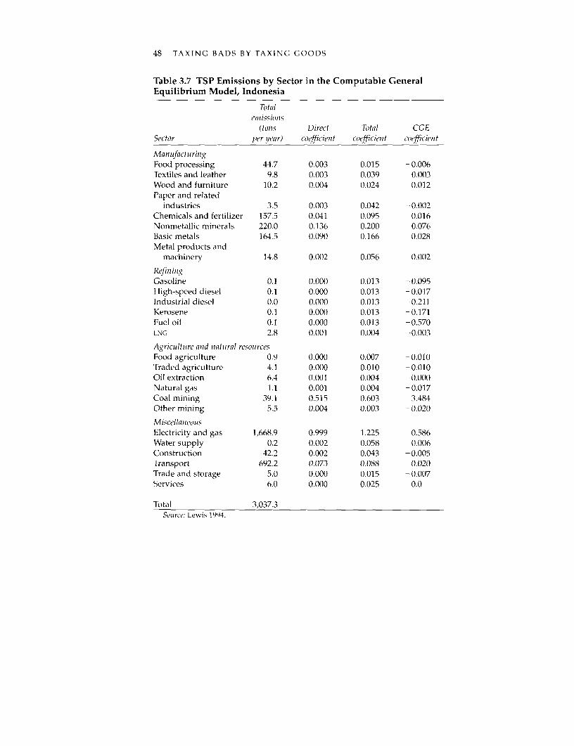
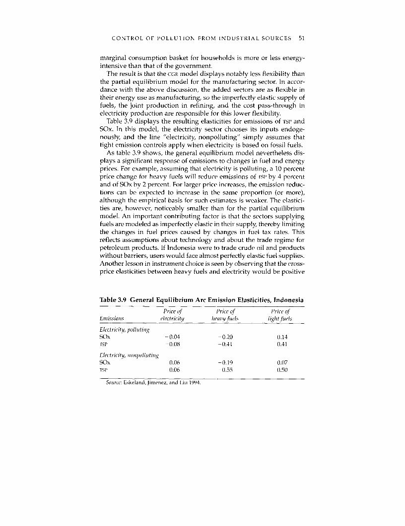
3 Control of Pollution from Industrial Sources 36General Economic Policies, Input and Output Taxes,

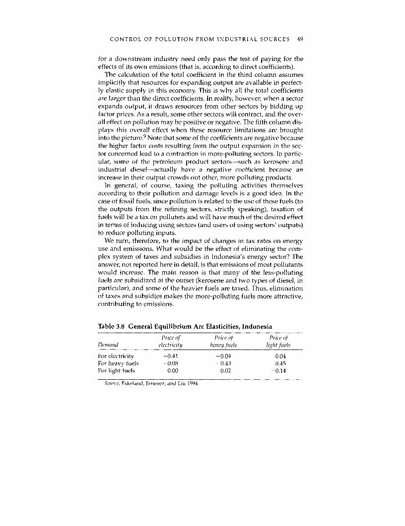
and Regulation 37Energy Conservation and Interfuel Substitution 39Exploration of General Equilibrium Effects 46Notes 53

4 Conclusion 55

Bibliography 57

iii

Preface

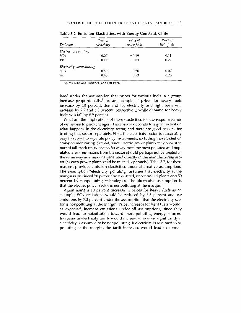
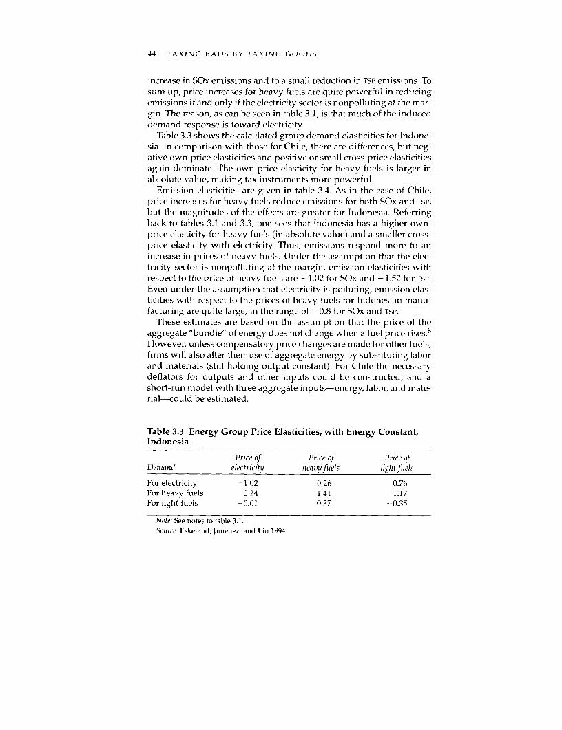
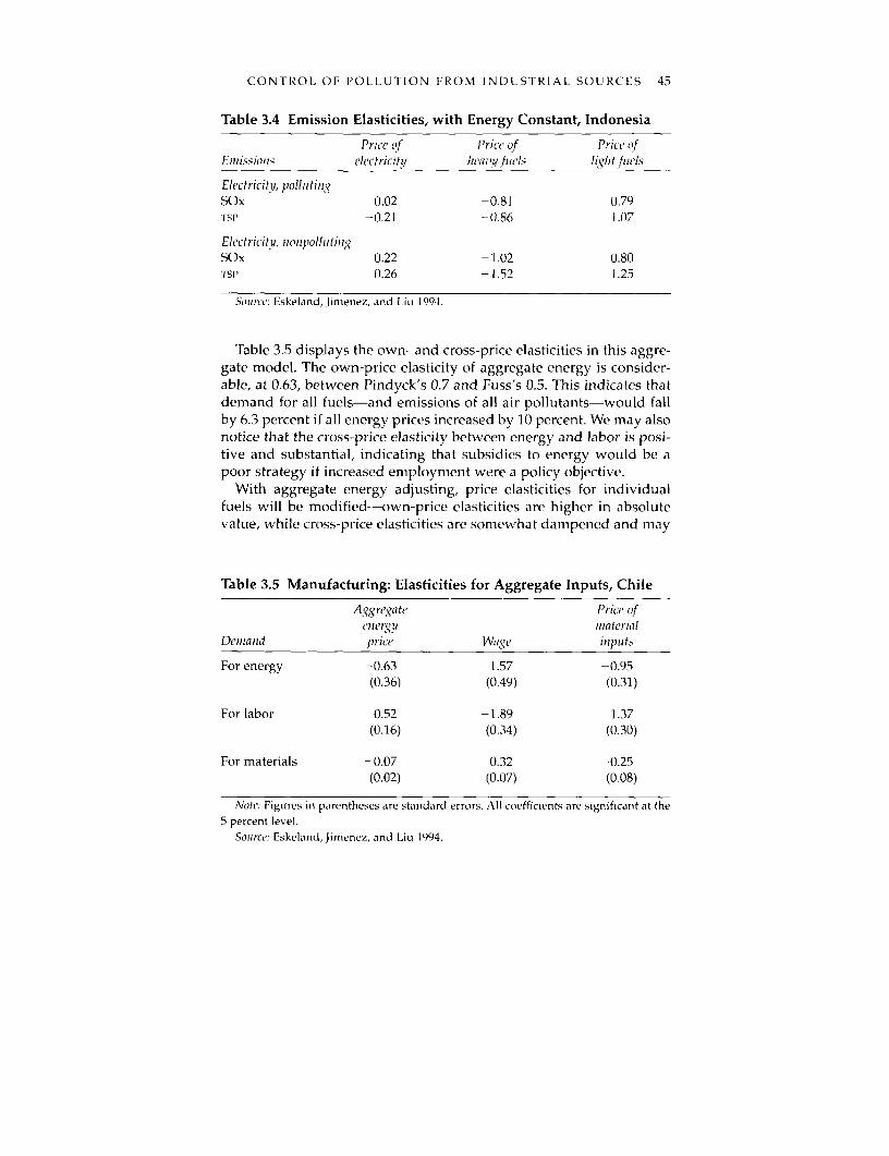
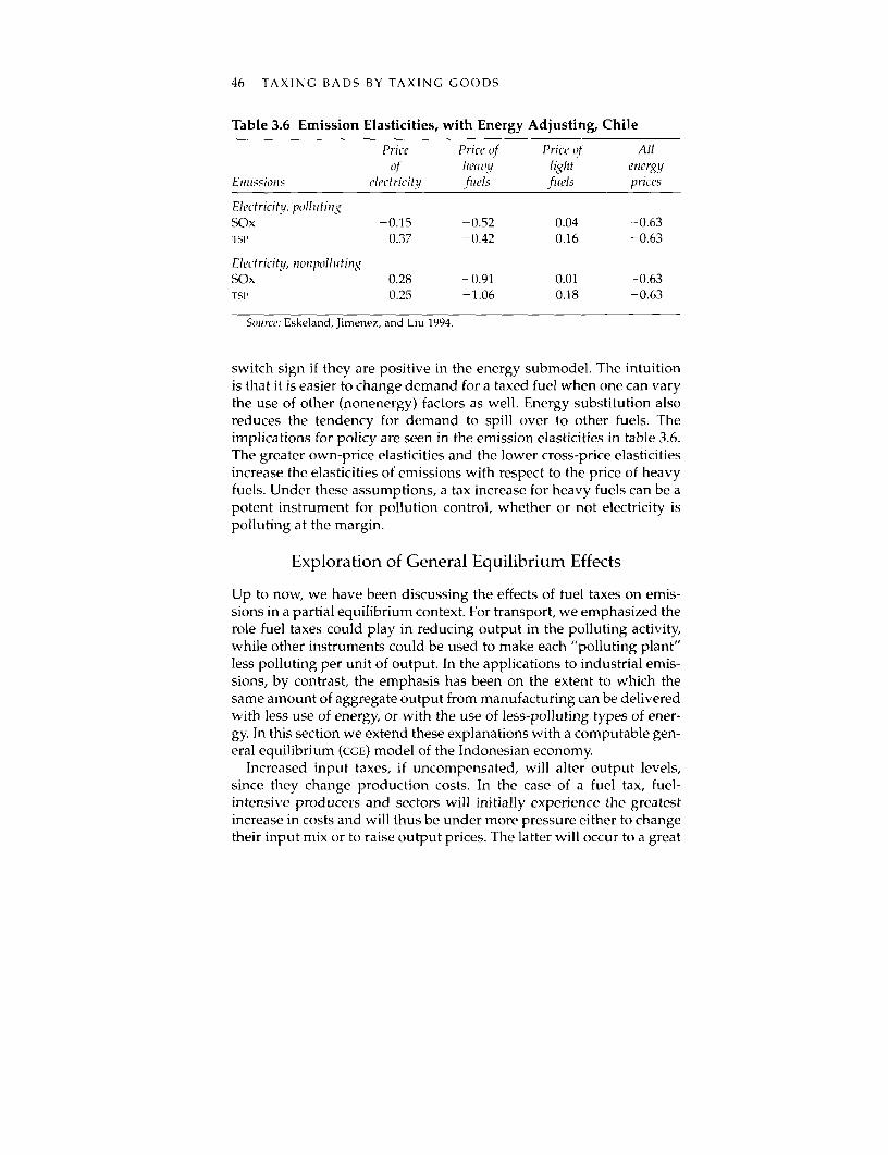
Solving environmental problems, in both developing and industrialcountries, appears to be more challenging than merely applying a fee onpolluters-a recommendation first put forth in Pigou's Economlics of Wel-fare (1920). One reason why the textbook remedy-levying an emissionfee on the polluter-has not been applied is that it requires the monitor-ing of individual emissions, which may be unrealistic in many situa-tions. In fact, most existing pollution control policies employ indirectinstruments-those that tax or regulate activities associated with emis-sions-rather than direct instruments based on individual emissions.

An important feature of the textbook solution is that the emissionfee gives the polluter an incentive to choose the optimal mix of cleanertechnologies and reductions in the scale of output or in the use ofinputs. When indirect instruments are used, this optimal combinationdoes not come about by itself. For instance, emission standards lead tocleaner cars and have modest monitoring requirements (annualinspections will do), but they do not effectively provide incentives forreducing the number of miles driven. The purpose of this book is toshow that indirect instruments designed to reduce the scale of outputcan be important complementary measures in a cost-effective pollu-tion control program. Examples of such instruments are taxes on out-put or on polluting inputs, called presimiptive because their target is thepollution presumed to be associated with the activity. A combinationof the two types of instruments-those that reduce output and thosethat reduce emissions per unit of output-can mimic fairly well theeffect of an optimal emission fee without the latter's monitoringrequirements. Specifically, when regulations requiring the adoption ofcleaner technologies are in place, the addition of a tax on an input asso-ciated with emissions can yield substantial benefits for a pollution con-trol program. These complementary instruments require very little orno additional resources for monitoring and enforcement. Furthermore,

V

vi TAXING BADS BY TAXING GOODS

schemes that make use of presumptive charges can be (and are likelyto be) refined as a country's monitoring capacity develops, so they arenot in conflict with "first-best" instruments.

Unlike the situation with emission fees, the optimal use of indirectinstruments requires knowledge concerning the "cleaner" technolo-gies (to determine the ease with which emissions per unit of outputcan be reduced) and the sensitivity of demand to prices (as an indica-tion of the ease with which output or input use can be reduced). Werely on case studies of Mexico City, Chile, and Indonesia to illustratethe choice between the two types of instruLments and the interactionbetween them.

A recurring theme throughout the book is that taxation of fuel usecan be a powerful indirect instrument for controlling air pollutionbecause of the association between fuel use and emissions. In the caseof automobiles, we show that failing to employ gasoline taxes in Mex-ico City would significantly reduce welfare, even when regulatorystandards are in place. In the case of point-source pollution, we calcu-late that there is significant potential for altering the fuel mix of indus-tries in Indonesia and Chile by taxing the "dirtier" fuels. Furthermore,for Indonesia we use a general equilibrium model to show that theconsequences of such a tax are similar to what is indicated in partialequilibrium models (although somewhat dampened). In sum, weadvocate taxing a "bad" (pollution) by taxing goods (fuels) as part ofa program to address air pollution when monitoring of emissions isprohibitively expensive.

Chapter 1 lays out our basic analytical framework. Chapter 2 treatsthe case of mobile-source pollution through an examination of gasolinetaxes and regulatory policies in Mexico City. Chapter 3 addresses point-source pollution and the potential for altering the fuel mix in industriesin Indonesia and Chile, based on firm-level data. A general equilibriummodel of Indonesia portrays the economywide consequences ofchanges in fuel taxes. Chapter 4 contains our concluding remarks.

The book distills the main results of a World Bank research project,"Pollution and the Choice of Policy Instruments." We are grateful toEmmanuel Jimenez, who developed the project jointly with GunnarEskeland and who provided advice, guidance, and comments. A short-er version of this book was presented at the 50th World Congress of theInternational Institute for Public Finance, Cambridge, Mass., August21-25, 1994, and appears in Bovenberg and Cnossen (1995). We thankCharles Ballard, Maureen Cropper, Gordon Hughes, and DavidWheeler for helpful comments. Peggy Pender and Hedy Sladovichprovided production assistance.

1. The Economics of PollutionControl: A Basic Analytical

Framework

To illustrate some important principles in the economics of pollutioncontrol, we begin with the textbook example of a polluting factory oran automobile-let us call it a plant-that produces a good (say, breador passenger-kilometers). Because the pollution emitted will harmpeople other than the plant manager, the marginal social cost of pro-duction exceeds its marginal private cost. The textbook solution to thisproblem is to levy a fee on pollutant emissions equal to the differencebetween the two costs (see box 1.1). The imposition of the emission feegives the plant manager an incentive to reduce emissions in two ways:by adopting cleaner technologies and by reducing output. Moreover,he will choose a combination of cleaner technologies and reduced out-put that is optimal not only for himself but also for society as a whole.Note that the policymaker need not know what this optimal combina-tion is-just as the purchaser of bread need not know the optimal com-bination of inputs required to produce it.

To make an emission fee work, however, the government has to mon-itor the plant's emissions. For many pollution problems, especiallythose caused by a large number of polluters, this is virtually impossi-ble. In this case, the government has two alternatives: tax the good pro-duced (or used) by the polluter, or ask the polluter to adopt a cleanertechnology. Below we show that each method contributes towardachieving the benefits of an emission fee, and that a good combinationof the two can mimic the effects of an emission fee reasonably well. Inthis situation, knowledge about control technologies and elasticities ofdemand for the polluting good is valuable to the policymaker. (Suchinformation is redundant if emissions can be monitored; polluters willuse their knowledge-and will volunteer the best response.)

The issue treated here is distinct from another that is popular in theliterature: the use of a market in pollution quotas or tradable permits.The use of emission quotas or permits, whether tradable or not,

I

2 TAXING BADS 13Y TAXING GOODS

Box 1.1 Behind the Textbook: Why Intervention Is Necessary

Under certain conditions, an undisturbed market will induce firms to useinputs and supply outputs efficiently. But the conditions under which themarket, without an intervening authority, will induce a firm to contain pol-lution efficiently are rare-mainly because the benefits of reduced residualsare public, shared by many.

The Coase theorem states that a firm will control pollution optimally if itnegotiates with the beneficiaries of pollution control, irrespective ofwhether the firm initially holds the right to pollute or, alternatively, the vic-tims hold the right to a clean environment. Let us first examine the situationin which polluters hold the right to pollute and victims must "bribe" pol-luters in order to reduce pollution. If the "victims" are numerous (as inMexico City, with 19 million people, or Greater Jakarta, with 15 million), avoluntary club to purchase emission reductions is likely to suffer from thefree-rider problem: nonmembers as well as members enjoy the benefits ofthe emission reductions. Then the purchases made by a voluntary club willbe backed by few, and pollution reduction will be suboptimal. The situationis not much better if polluters initially hold no right to pollute but have tobuy emission permits from the victims of pollution. An individual holdingsuch rights will sell his with a light heart (even at a low price), since he willsuffer only a minuscule share of the consequences in terms of pollutionincreases. Others will also suffer, without sharing in the revenues from thistransaction. In both cases it is the "publicness" of the environmental goodthat makes voluntary negotiations so impotent, and in both cases applica-tion of authority can solve the problem.

If we view the municipality as a citizen-minded club in which member-ship is compulsory, the pollution control agency can be seen as its repre-sentative, with power to negotiate with polluters. In that situation the Coasetheorem ensures efficient pollution control and optimal pollution levels,with fees or permits that reflect a "social contract."

requires the pollution control agency to monitor individual firms'emissions. Hence, if monitoring of emissions is difficult, the problemcannot be solved by allowing trade in quotas. Nevertheless, onlyunder certain conditions will problems with monitoring make the useof market forces in a control program a poor proposition. Note furtherthat we are concerned here with cost-efficient pollution control; that is,we do not attempt to quantify the benefits from pollution reduction.Rather, we take the targeted level of pollution reductions as given andlook for the least costly means of achieving it. (Benefit estimates can beuseful as priority weights in cost-effectiveness analysis when multiple

THE ECONOMICS OF POLLUTION CONTROL 3

pollutants are addressed. Box 1.2, later in the chapter, presents a sum-mary of such estimates.)

The Textbook Case: An Emission Fee

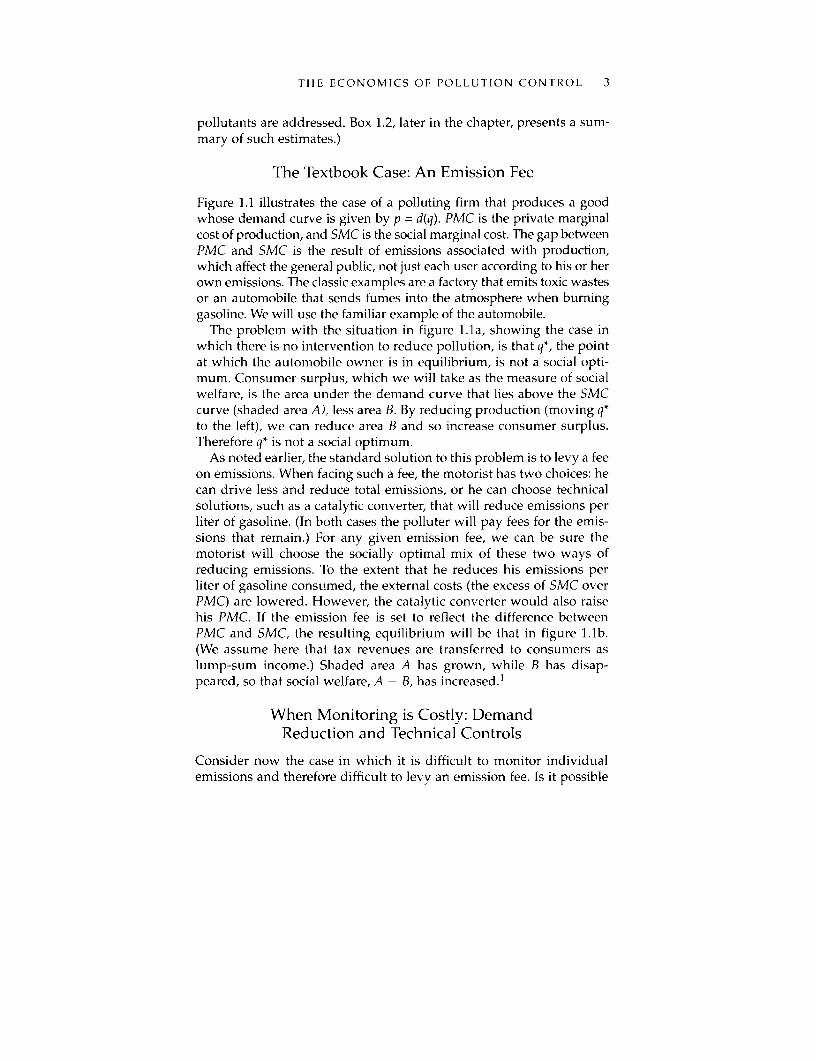
Figure 1.1 illustrates the case of a polluting firm that produces a goodwhose demand curve is given by p = d(q). PMC is the private marginalcost of production, and SMC is the social marginal cost. The gap betweenPMC and SMC is the result of emissions associated with production,which affect the general public, not just each user according to his or herown emissions. The classic examples are a factory that emits toxic wastesor an automobile that sends fumes into the atmosphere when burninggasoline. We will use the familiar example of the automobile.

The problem with the situation in figure 1.1a, showing the case inwhich there is no intervention to reduce pollution, is that q*, the pointat which the automobile owner is in equilibrium, is not a social opti-mum. Consumer surplus, which we will take as the measure of socialwelfare, is the area under the demand curve that lies above the SMCcurve (shaded area A), less area B. By reducing production (moving q*to the left), we can reduce area B and so increase consumer surplus.Therefore q* is not a social optimum.

As noted earlier, the standard solution to this problem is to levy a feeon emissions. When facing such a fee, the motorist has two choices: hecan drive less and reduce total emissions, or he can choose technicalsolutions, such as a catalytic converter, that will reduce emissions perliter of gasoline. (In both cases the polluter will pay fees for the emis-sions that remain.) For any given emission fee, we can be sure themotorist will choose the socially optimal mix of these two ways ofreducing emissions. To the extent that he reduces his emissions perliter of gasoline consumed, the external costs (the excess of SMC overPMC) are lowered. However, the catalytic converter would also raisehis PMC. If the emission fee is set to reflect the difference betweenPMC and SMC, the resulting equilibrium will be that in figure 1.1b.(We assume here that tax revenues are transferred to consumers aslump-sum income.) Shaded area A has grown, while B has disap-peared, so that social welfare, A - B, has increased.'

When Monitoring is Costly: DemandReduction and Technical Controls

Consider now the case in which it is difficult to monitor individualemissions and therefore difficult to levy an emission fee. Is it possible

4 TAXING BADS BY TAXING GOODS

Figure 1.1 A Polluting Firm: Four Scenarios

(a) No intervention (b) A pollution taxConsumer surplus (A - B) (or output tax and abatement)

Consumer surplus = A

Price Price(j)) (P)

SMC ------- SMC

Demand-PMC

Quantity Quantity

(c) Pollution tax on output (d) Mandated abatementConsumer surplus = A Consumer surplus = (A - B)

Price Price(P) (P)

A\SMC A-M-------------SMC

'\ PMC x IMC'-. - - <- - - -PMC

Quantity Quantity

to achieve some or all the benefits of an emission fee by using othermeans to curtail demand or induce technical controls?

The first possibility is illustrated in figure 1.1c, where we haveimposed a tax on output (or on a variable input such as gasoline) equalto the difference between social and private marginal costs. The taxinduces consumers to reduce their consumption by manipulating theprice that they face.2 Consumer surplus, in this case, will be area A. Soci-ety has made net gains equal to B in figure l.la by eliminating the con-sumption for which marginal social costs exceeded marginal social ben-efits. Note that the social savings from such a strategy (area B in figure1.1a) depend crucially on the slope of the demand curve: the steeper the


curve, the smaller the gains from demand-management instrumentssuch as input and output taxes. However, the size of the optimal tax isindependent of the slope of the demand curve whenever the differencebetween SMC and PMC is constant.

In figure 1.1c we assume that a tax on a commodity such as gasolinewould suppress demand in a "neutral" fashion-not changing theamount of pollution per liter of gasoline consumed. In figure 1.1b weassume that an emission control technology, such as a catalytic con-verter, is available. The application of the technology would increasethe private marginal costs from PMC to PMC' but would also reducepollution per unit so much as to position the new social marginal costcurve, SMC, below the original one.

Figure I.Id displays what happens if the adoption of such a tech-nology is induced directly-for instance, by regulation. First, as socialmarginal costs are shifted downward, area A expands and area Bshrinks. Second, since consumers now face a private marginal cost thatincludes the costs of catalytic converters, consumption is also reduced(in comparison with figure 1.1a), and so area B is further reduced. Con-sumer surplus (A - B) will necessarily be greater than in the uncon-trolled case.

Finally, consider what happens when mandated abatement is com-bined with a gasoline tax that is optimal under a specific abatementtechnology. We introduce a tax to suppress the consumption that isexcessive, taking into account the reduced emission coefficient. Thenew equilibrium is identical to that achieved by an emission tax in fig-ure 1.1b. In comparison with figure 1.1c, we have introduced man-dated abatement to make consumption cleaner. Taxes on the pollutinggood are therefore lower, and we can benefit from additional con-sumption. Note that area A is bigger and the gasoline tax per liter ofgasoline is smaller. However, the tax rate per unit of pollution is thesame in figures 1.1a and c; the difference in tax rates per liter merelyreflects the difference in emissions per liter.

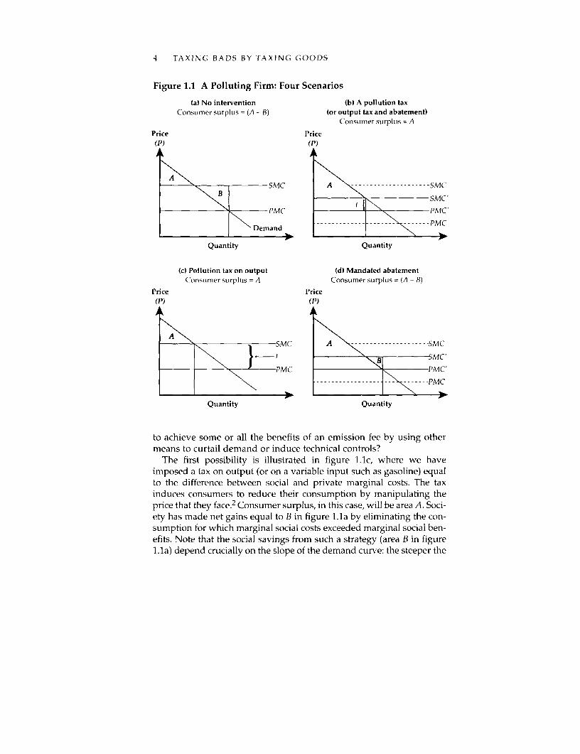
When a polluter can "go in two different directions"-abatement orreduced activity levels-to reduce pollution, the problem is bestdescribed in three dimensions. Figure 1.2 portrays the cost structure interms of private marginal costs and social marginal costs. The twocurves along the output line are traditional marginal cost curves withno abatement applied: the PMC curve, with no inclusion of the dam-ages caused by pollution, and the SMC curve, including the externalcosts of the pollution. Along the abatement axis, we can see that pri-vate marginal costs increase monotonously, while the social marginalcosts first decrease, then increase. The reason is that abatement is effec-


Figure 1.2 Determination of Abatement

A iCost, price i

_ _ __ _ _ __ _ __ _ _ __ _ __ _ / >expansion

Output

tive in reducing emissions, and initially at such a rate that the reduceddamages are more than sufficient to justify the private costs of abate-ment. When the SMC surface eventually turns upward, it means thatzero pollution is "too little"-because reductions eventually cost toomuch in terms of abatement costs. The "optimal expansion path,"depicting the projection vertically under the "valley bottom" of socialmarginal costs, describes the socially optimal way of producing out-put, for a range of output levels.

In figure 1.3 the cost structure is brought together with demand. Thetraditional demand curve, now a "demand surface," is sliced vertical-ly along the lines of zero abatement and along the optimal expansion


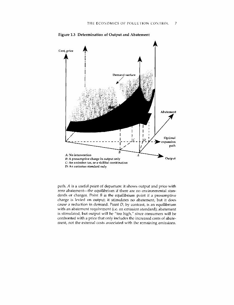
Figure 1.3 Determination of Output and Abatement

Cost, price 4

Demand surface

Abatement

I Optimal- _. __expansion

path

BA: No intervention AB: A presumptive charge in output only OutputC: An emission tax, or a skillful combinationD: An emission standard only

path. A is a useful point of departure: it shows output and price withzero abatement-the equilibrium if there are no environmental stan-dards or charges. Point B is the equilibrium point if a presumptivecharge is levied on output: it stimulates no abatement, but it doescause a reduction in demand. Point D, by contrast, is an equilibriumwith an abatement requirement (i.e. an emission standard); abatementis stimulated, but output will be "too high," since consumers will beconfronted with a price that only includes the increased costs of abate-ment, not the external costs associated with the remaining emissions.


Point C displays optimal abatement and output, which can be reachedwith the use of direct instruments such as charges levied directly onemissions, or approximated with skillful combinations of abatementrequirements and presumptive charges levied on output.

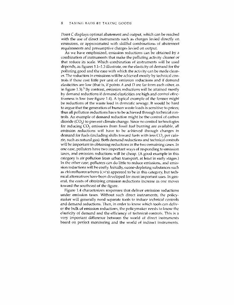
As we have emphasized, emission reductions can be obtained by acombination of instruments that make the polluting activity cleaner orthat reduce its scale. Which combination of instruments will be useddepends, as figures 1.1-1.3 illustrate, on the elasticity of demand for thepolluting good and the ease with which the activity can be made clean-er. The reduction in emissions will be achieved mostly by technical con-trols if these cost little per unit of emission reductions and if demandelasticities are low (that is, if points A and D are far from each other, asin figure 1.3).3 By contrast, emission reductions will be attained mostlyby demand reductions if demand elasticities are high and control effec-tiveness is low (see figure 1.4). A typical example of the former mightbe reductions of the waste load in domestic sewage. It would be hardto argue that the generation of human waste loads is sensitive to prices;thus all pollution reductions have to be achieved through technical con-trols. An example of demand reduction might be the control of carbondioxide (CO2 ) to prevent climate change. Since no control technologiesfor reducing CO2 emissions from fossil fuel burning are available, allemission reductions will have to be achieved through changes indemand for fuels (including shifts toward fuels with less CO, per calo-rie, such as natural gas). Both demand reductions and technical controlswill be important in obtaining reductions in the two remaining cases. Inone case, polluters have two important ways of responding to emissiontaxes, and emission reductions will be cheap. (A good example in thiscategory is air pollution from urban transport, at least in early stages.)In the other case, polluters can do little to reduce emissions, and emis-sion reductions will be costly. Initially, ozone-depleting substances suchas chlorofluorocarbons (CFCs) appeared to be in this category, but tech-nical alternatives have been developed for most important uses. In gen-eral, the costs of obtaining emission reductions increase as one movestoward the southeast of the figure.

Figure 1.4 characterizes responses that deliver emission reductionsunder emission taxes. Without such direct instruments, the policy-maker will generally need separate tools to induce technical controlsand demand reductions. Then, in order to know which tools can deliv-er the bulk of emission reductions, the policymaker needs to know theelasticity of demand and the efficiency of technical controls. This is avery important difference between the world of direct instrumentsbased on perfect monitoring and the world of indirect instruments.


Figure 1.4 How Most Emission Reductions Are Delivered When...

High Low

- Demannd reduction Both

Simply put, if the pollution control agency knows little about individ-ual emissions, then it should know much about other things, such aswhat characterizes polluters and what options are available to them.Figure 1.5 summarizes wlhich indirect instrument will be most impor-tant in providing emission reductions, on the basis of the same under-lying conditions as in figure 1.4.

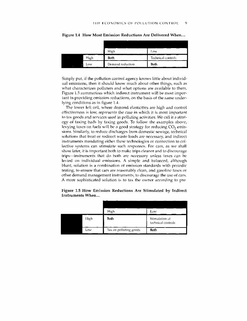
The lower left cell, where demand elasticities are high and controleffectiveness is low, represents the case in which it is most importantto tax goods and services used in polluting activities. We call it a strat-egy of taxing bads by taxing goods. To follow the examples above,levying taxes on fuels will be a good strategy for reducing CO, emis-sions. Similarly, to reduce discharges from domestic sewage, technicalsolutions that treat or redirect waste loads are necessary, and indirectinstruments mandating either these technologies or connection to col-lective systems can stimulate such responses. For cars, as we shallshow later, it is important both to make trips cleaner and to discouragetrips-instruments that do both are necessary unless taxes can belevied on individual emissions. A simple and balanced, althoughblunt, solution is a combination of emission standards with periodictesting, to ensure that cars are reasonably clean, and gasoline taxes orother demand management instruments, to discourage the use of cars.A more sophisticated solution is to tax the owner according to pre-

Figure 1.5 How Emission Reductions Are Stimulated by IndirectInstruments When...

I High Low

inBoth Stimulation oftechnical controls

Tax on polluting goods Both


sumed accumulated emissions. The latter proposal-which wouldgive much better incentives to owners and users-has yet to beapplied in practice.

It should be noted that combinations of instruments are useful in allthe cells; the emphasis here is on which instruments are most impor-tant. Another way of reading the grid is to ask when it is costly toapply only a narrow range of instruments. For instance, a programconsisting only of instruments stimulating emission control technolo-gies will be a costly one, and unnecessarily so, if demand elasticitiesare high. (Such narrow programs are the rule, rather than the excep-tion, in practice.) Similarly, a program consisting only of input taxeswill be costly if emission control technologies would be effective inreducing emissions per unit of input.

Presumptive Charges: Problems and Promises

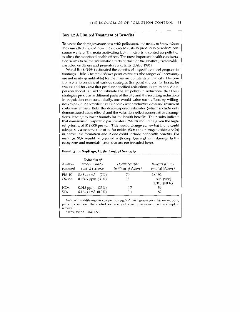
A Pigovian tax on emissions that is equal to external damages wouldgenerally be the first-best policy prescription. Box 1.2 summarizes con-servative estimates for the health benefits of air pollution reductions inSantiago, Chile.4 We have argued that taxes can also be levied on pol-luting goods and services, in presumption of emissions associatedwith their use. However, because the link between external damagesand the use of polluting goods and services may be weak, marginalemissions may vary among polluters paying the same presumptivecharges. In brief, the incentives provided by presumptive taxes willinherit any weakness in the association between the tax base (such asfuel consumption) and damages.

On the control side, because each option typically involves severalpollutants, benefits and control costs can best be compared by strategyrather than by pollutant. The analysis shows that health benefits alonecan justify all four strategies. The two with the highest benefit-costratios are the fixed-source strategy (mostly because of its particlereductions) and the car strategy (mostly for its ozone reductions).

We use an example to illustrate the problems-and the strategies-associated with presumptive instruments. Let emissions from polluter i,e', be determined by the quantity consumed of a polluting good, x', andalso by a parameter describing the type of technology, ai. The cost to thepolluter of a price increase of $1 for the polluting good is equal to thenumber of units used, x'. The change in tax proceeds received by thegovernment (assuming that other goods are untaxed) is x' + txt, where asubscript stands for partial derivatives, so that x, denotes the marginalchange in demand in response to the tax increase.5 Thus, if we assume


Box 1.2 A Limited Treatment of Benefits

To assess the damages associated with pollutants, one needs to know whomthey are affecting and how they increase costs to producers or reduce con-sumer welfare. The main motivating factor in efforts to control air pollutionis often the associated health effects. The most important health considera-tion seems to be the systematic effects of dust, or the smallest, "respirable"particles, on illness and premature mortality (Ostro 1994).

World Bank (1994) estimated the benefits of a specific control program inSantiago, Chile. The table shows point estimates (the ranges of uncertaintyare not easily quantifiable) for the main air pollutants in that city. The con-trol scenario consists of various strategies (for point sources, for buses, fortrucks, and for cars) that produce specified reductions in emissions. A dis-persion model is used to estimate the air pollution reductions that thesestrategies produce in different parts of the city and the resulting reductiolnsin population exposure. Ideally, one would value such effects by willing-ness to pay, but a simplistic valuation by lost productiv e days and treatmentcosts was chosen. Both the dose-response estimates (which include onlydemonstrated acute effects) and the valuation reflect conservative assump-tions, leading to lower bounds for the health benefits. The results indicatethat emissions of respirable particulates (PM-10) should be given the high-est priority, at $18,000 per ton. This would change somewhat if one couldadequately assess the role of sulfur oxides (SOx) and nitrogen oxides (NOx)in particulate formation and if one could include nonhealth benefits. Forinstance, SOx would be credited with crop loss and with damage to theecosystem and materials (costs that are not included here).

Benefits for Santiago, Chile, Control Scenario

Reduction ofAmwbient exposure under Healtli bensefits Ben.efits per tollpollutant control scenario (nillions of dollars) emitted (dollars)

PM-10 8.43iLg/m 3 (70/o) 70 18,192Ozone 0.0365 ppm (33%.) 33 495 (voc)

1,315 (NOx)NOx 0.013 ppm (33%) 0.7 59SOx 0.16[Lg/m 3 (0.3%) 0.1 82

Note: voc, volatile organic compounds; hLg/n 3 , micrograms per cubic meter; ppm,parts per million. The control scenario yields an improvement, not a completeremoval.

Souirce: World Bank 1994.


that income is worth the same whether it accrues to the government orto the polluter, the social cost of raising the tax rate is tx,'. The marginalchange in emissions from polluter i in response to a change in the taxrate will be e. xi + e', a,. Assuming, perhaps conservatively that technol-ogy does not change in response to a price increase for the pollutinginput (na, = 0), the marginal social cost of emission reductions producedby a price change for the polluting good is

(1.1) t/e'

or, simply, the tax rate divided by the marginal emission factor, aver-aged over polluters (the latter may depend on technology as well as onconsumption).

There are two problems with such a presumptive charge on a pol-luting good. One is related to the failure of t effectivelv to stimulateother initiatives that can reduce emissions, here represented by thevariable a'.6 As noted above, one may address this problem by usingseparate instruments (incentives or regulation) to induce the applica-tion of cleaner technologies, depending on how attractive these areand on their monitoring and enforcement requirements. At givenabatement levels, however, marginal cost expressions like equation 1.1apply as long as the emission factor reflects the abatement level. Thus,when taking into account the estimated marginal emission factors,appropriately averaged if there are many polluters, one can reduceemissions by raising the price of the polluting input at a marginal costindicated by equation 1.1.

The other problem with the presumptive tax levied on a pollutinginput is that it is "unfair," and in a way that is also inefficient: it dis-courages the use of the polluting good with the same strength (as mea-sured by the tax rate) for polluters who may have different emissionfactors. Thus, while a polluter with a high emission factor couldreduce emissions cheaply by reducing her use of the polluting good,she will have only average inducements for doing so as long as shefaces the same tax on the polluting good as others. This may be a prob-lem even if separate strategies can be pursued to induce cleaner tech-nology, since emission factors may vary even wheni separate instru-ments push abatement optimally.

Thus, if one recommends presumptive taxation of polluting inputsand goods in lieu of high monitoring and enforcement costs, theseweaknesses have to be kept in mind. An important point is that anincentive scheme based mainly on presumptive charges can be com-plemented and refined as technical and institutional capacity allows.


Because of these weaknesses, presumptive taxes are not themselvespart of an ideailized incentive scheme (a hypothetical scenario with cost-less monitoring). They may provide a setting conducive to institution-al and policy development in the direction of the ideal system-a set-ting sensitive to the practical challenge of developing monitoringcapacity. The argument rests on the observation that presumptivecharges are both "unfair" and "transfer-intensive." "Unfairness" willinduce polluters that are or can be cleaner than average to self-report,citing their lower emission factors to justify refunds of parts of thetaxes paid or simply lower tax rates. Incentives to do so are high, sincethe taxpaying polluter regards the transfer she makes to the govern-ment as a cost and any savings as 100 percent genuine savings. Thepollution control agency can announce, when it is institutionally andtechnically capable, that special treatment, such as partial refunds, isavailable for those who prove cleaner than average. It would then beup to the polluter to take the initiative. She can support the claim thatshe is cleaner than average by self-reporting, by credible monitoring,and by submitting to special audit regimes. Such a policy refinementwould provide incentives both for pollution abatement technologiesand for monitoring and auditing technologies. As polluters with loweremission coefficients opt out of the "basket case" treatment, the taxrate for the remaining polluters will increase (since their weighted-average emission factors increase). Starting from a basis of crude pre-sumptive instruments, the policy stance described here could lead inthe direction of a very sophisticated emission fee system.

This "policy trajectory" argument carries some risks, however. Theincentives provided by blunt presumptive charges (and those pro-vided by environmental regulation, which will also be based on aver-ages) may remain rigid and blunt, rather than continuously refined.The pollution control agency (and the treasury), infatuated by pro-ceeds from taxes on polluting goods, may resist calls for special treat-ment, since they come from polluters who would like to pay less. Also,rigidity and tiniformity may be seen as virtues in some bureaucracies.Polluters, if they expect a negative or undifferentiated response, willnot have an additional incentive to become cleaner than the average.The latter risk is higher if the taxes are perceived as ordinary indirecttaxes, rather than as a specific charge that polluters are invited to avoidthrough specific avenues. It should be remembered, however, that pre-sumptive charges serve a purpose in pollution control even if theyremain blunt instruments, as long as they do not block development ofthe more refined incentive schemes.


Notes

1. The assumption essential to this argument is that the value of public rev-enue is equal to that of private incomes. Assuming (costless) lump-sum trans-fers is one way of ensuring this equivalence, and an assumption of marginalutilities of income independent of the price of the polluting good allows theuse of consumer surplus as a measure of welfare costs. For analysis in a con-text with (optimal) distortionary taxes, see Sandmo (1975).

2. If an input tax is envisaged, the argument in this section assumes fixedcoefficients of that input to output; that is, the gasoline tax can reduce the useof the car but cannot make car use less fuel-intensive. This assumption and itsrelaxation are discussed in detail in the next two chapters.

3. Technical controls and cleaner consumption are here used svnonymous-ly; what is essential is that emissions are reduced per unit of input or output.Technical controls show high effectiveness if they can shift emissions down-ward so that the SMC curve is shifted downward sharply. Because the SMCcurve denotes the sum of PMC and the external costs due to emissions, thisshift is possible only if emissions can be reduced sharply without a majorincrease in PMC.

4. On the importance of health concerns for air pollution control policies, seeFreeman (1982) and Pearce and Markandva (1986). On health effects, see Ostro(1994) for a review and, for estimates from developing countries, Alberini,Harrington, and McConnell (1994), Alberini and others (1995), Eskeland andothers (forthcoming), and Ostro and others (1995).

5. The argument also holds for another setting for nondistortionary taxa-tion: when all goods are otherwise optimally taxed at uniform ad valoremrates (no distortionarv taxation). In that case, the tax rate here referred to as thetax rate, t. on the poliuting good should be interpreted as a special additionalunit rate. Note that we assume that the production cost of the polluting goodis given; thus the change in the user cost is the same as the change in the taxrate.

6. Replacement of older, dirtier machinerv by newer, cleaner machinerv willoften be accelerated by increased fuel prices, but this does not mean that fuelprices are effective in stimulating cleaner technologies.

2. Pollution from Mobile Sources

A pollution control agency able to levy taxes on each individual's emis-sions need not know anything about the technical and behavioralchanges that could produce pollution reductions. The agency would bein a position analogous to that of a buyer of fruit who is confident of hisability to assess the produce upon arrival. The buyer pays whoever offersgood produce; he has no interest in the background of the suppliers orthe history of their shipments. But what if fruit for the city mysteriouslylanded on the mayor's doorstep at night? He would be hesitant aboutpaying those claiming to be responsible the following morning, just as hewould be hesitant about paying a rainmaker without further evidence.

Similarly, if a social planner possessed data on how much pollutioneach individual caused throughout the year, a year-end tax bill basedon emissions would easily provide appropriate incentives for pollu-tion reduction; only those who had polluted would contribute to thepollution control program. For many important pollution categories,however, including motor vehicles, emissions are not monitored con-tinuously-and will not be, in the near future. In this situation, theplanner needs to investigate which sectors are polluting, what optionsexist withini each sector, and how he can best stimulate them.

Using Indirect Instruments: Cleaner Cars, Fewer Trips

Let us initially accept the proposition that the planner has a monitor-ing problem: he does not know how much pollution each individualemits throughout the year and thus cannot, with full precision andwithout cost, levy a charge directly on individual emissions. With indi-rect instruments, he will often have to apply separate strategies to pro-mote the various ways by which polluters can curb emissions. We mayview the pollution control agency as an agent who purchases emissionreductions on behalf of the public (see box 1.1 in the last chapter). To

15


such an agent, cleaner cars and fewer trips are alternative suppliers ofemission reductions, and she should buy from each up to the point atwhich emission reductions, at the margin, cost the same from each.'

We now consider a traditional control program that focuses on mak-ing cars cleaner and ask whether and how such a program can be com-bined with a uniform gasoline tax. The role of the gasoline tax is to pro-vide polluters with an incentive to reduce their demand for thepolluting good. The principal weakness of such a reform is that it dis-courages vehicle use uniformly, ignoring differences in emission rates.The practical reason for suggesting such a modest reform is the gener-al suspicion that administrative and technical systems for emission test-ing are still vulnerable (see box 2.3, below), raising doubts as towhether they should be used as major tax-collecting devices. The beau-ty of the fuel tax is its administrative simplicitv: all countries interferein fuel markets (some with a tax, others with a subsidy), so their abili-ty to manipulate this price is proven. The collection of a pollution-moti-vated charge in fuel markets requires little or no new monitoring.

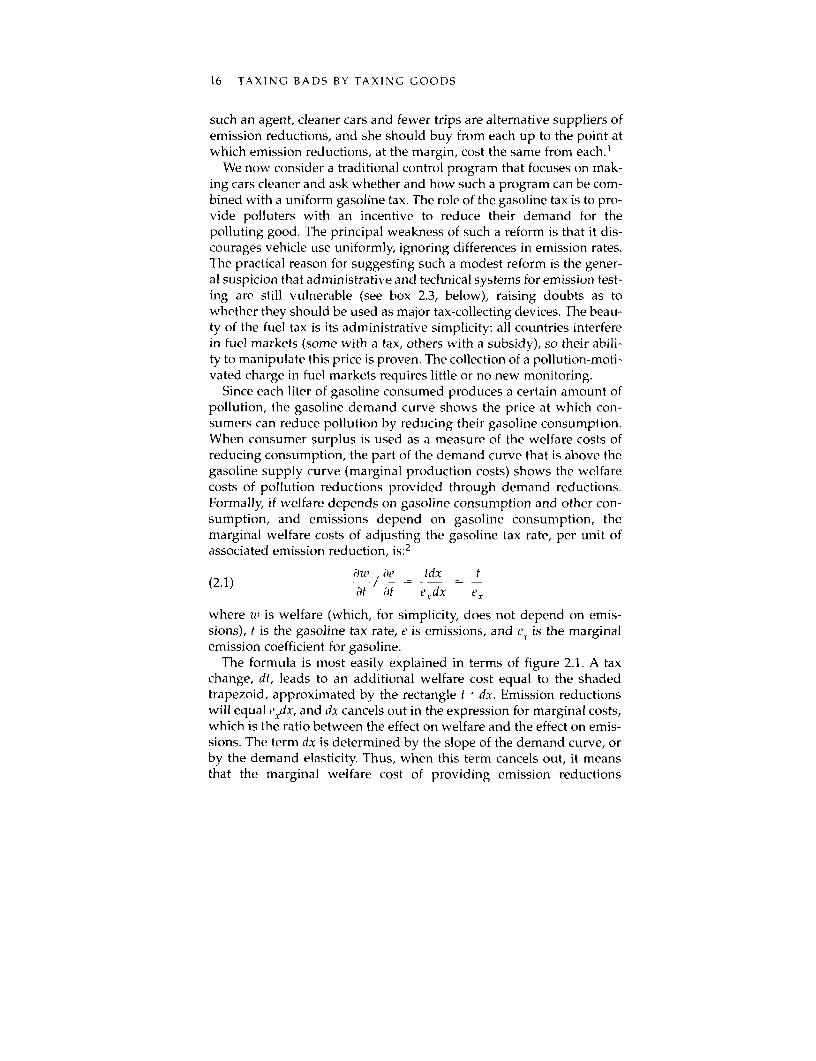
Since each liter of gasoline consumed produces a certain amount ofpollution, the gasoline demand curve shows the price at which con-sumers can reduce pollution by reducing their gasoline consumption.When consumer surplus is used as a measure of the welfare costs ofreducing consumption, the part of the demand curve that is above thegasoline supply curve (marginal production costs) shows the welfarecosts of pollution reductions provided through demand reductions.Formally, if welfare depends on gasoline consumption and other con-sumption, and emissions depend on gasoline consumption, themarginal welfare costs of adjusting the gasoline tax rate, per unit ofassociated emission reduction, is:2

a3n' ie _ tdx __t

(2.1) 1-----_tdr at at e .dx e,

where w' is welfare (which, for simplicity, does not depend on emis-sions), t is the gasoline tax rate, e is emissions, and e. is the marginalemission coefficient for gasoline.

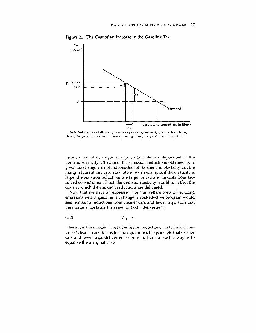
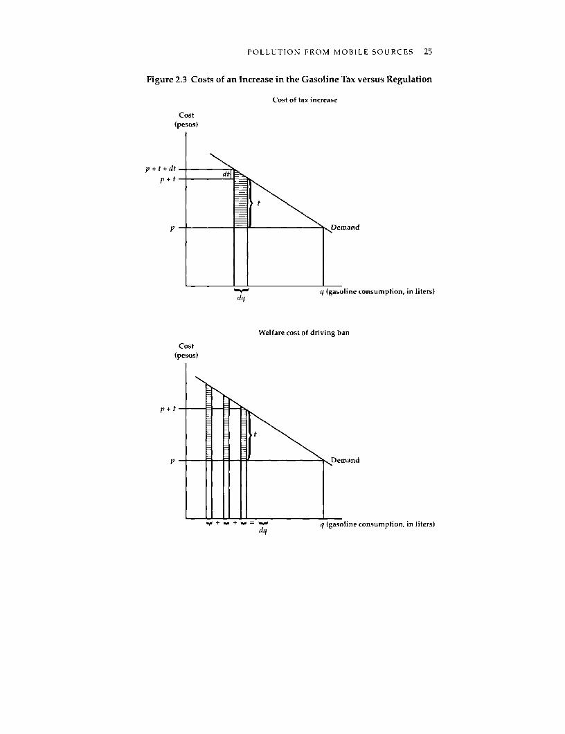
The formula is most easily explained in terms of figure 2.1. A taxchange, dt, leads to an additional welfare cost equal to the shadedtrapezoid, approximated by the rectangle t * dx. Emission reductionswill equal c_dx, and dx cancels out in the expression for marginal costs,which is the ratio between the effect on welfare and the effect on emis-sions. The term dx is determined by the slope of the demand curve, orby the demand elasticity. Thus, when this term cancels out, it meansthat the marginal welfare cost of providing emission reductions

POLLUTION FROM MOBILE SOURCES 17

Figure 2.1 The Cost of an Increase in the Gasoline Tax

Cost(pesos)

p +t+d- dti

p+tt

Demand

x (gasoline consumption, in liters)dx

Note: Values are as follows: p, producer price of gasoline; t, gasoline tax rate; dt,change in gasoline tax rate; dx, corresponding change in gasoline consumption1.

through tax rate changes at a given tax rate is independent of thedemand elasticity. Of course, the emission reductions obtained by agiven tax change are not independent of the demand elasticity, but themarginal cost at any given tax rate is. As an example, if the elasticity islarge, the emission reductions are large, but so are the costs from sac-rificed consumption. Thus, the demand elasticitv* would not affect thecosts at which the emission reductions are delivered.

Now that we have an expression for the welfare costs of reducingemissions with a gasoline tax change, a cost-effective program wouldseek emission reductions from cleaner cars and fewer trips such thatthe marginal costs are the same for both "deliveries":

(2.2) tlex = c

where c, is the marginal cost of emission reductions via technical con-trols ("cleaner cars"). This formula quantifies the principle that cleanercars and fewer trips deliver emission reductions in such a way as toequalize the marginal costs.


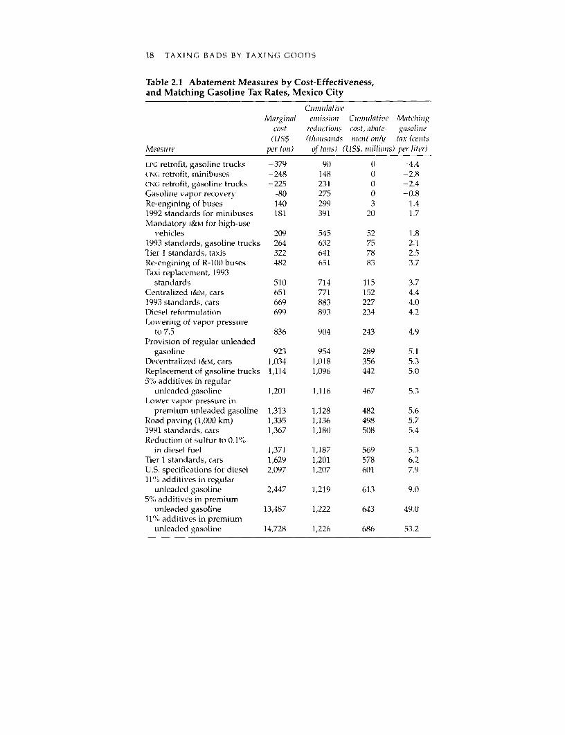
Table 2.1 Abatement Measures by Cost-Effectiveness,and Matching Gasoline Tax Rates, Mexico City

ClulmllalfiveMlarginal emiissioni Curmlnative Matchliing

cost rednictionis cost, abate- gasoline(US$ (thousa171tns 11117n1t otnly taX (celnts

Measiure per toW) of tonis) (US$, mttillionis) per liter)

LPG retrofit, gasoline trucks -379 90 0 -4.4CNG retrofit, minibuses -248 148 0 -2.8CNG retrofit, gasoline trucks -225 231 0 -2.4Gasoline vapor recovery -80 275 0 -0.8Re-engining of buses 140 299 3 1.41992 standards for minibuses 181 391 20 1.7Mandatory j&Mi for high-use

vehicles 209 545 52 1.81993 standards, gasoline trucks 264 632 75 2.1Tier I standards, taxis 322 641 78 2.5Re-engining of R-100 buses 482 651 83 3.7Taxi replacement, 1993

standards 510 714 115 3.7Centralized i&M, cars 651 771 152 4.41993 standards, cars 669 883 227 4.0Diesel reformulation 699 893 234 4.2Lowering of vapor pressure

to 7.5 836 904 243 4.9Provision of regular unleaded

gasoline 923 954 289 5.1Decentralized i&M, cars 1,034 1,018 356 5.3Replacement of gasoline trucks 1,114 1,096 442 5.05% additives in regular

unleaded gasoline 1,201 1,116 467 5.3Lower vapor pressure in

premium unleaded gasoline 1,313 1,128 482 5.6Road paving (1,000 km) 1,335 1,136 498 5.71991 standards, cars 1,367 1,180 508 5.4Reduction of sulfur to 0.1%

in diesel fuel 1,371 1,187 569 5.3Tier 1 standards, cars 1,629 1,201 578 6.2U.S. specifications for diesel 2,097 1,207 601 7.911%.o additives in regular

unleaded gasoline 2,447 1,219 613 9.05% additives in premium

unleaded gasoline 13,487 1,222 643 49.011%.;, additives in premium

unleaded gasoline 14,728 1,226 686 53.2


Note to table 2.1

Note: i Rn, liquefied petroleum gas; CNG, compressed natural gas; I&M, inspectionand maintenance. The first and second columns give, respectively, the height andlength of the steps on the technical control cost curve shown in figure 2.2. The match-ing gasoline tax (equation 2.2) shown in the last column increases monotonously pergram of pollutants but not per liter of gasoline, since emissions per liter (cx) arebrought down progressively by controls.

Source: Eskeland 1994b.

What if a pollution control program did not follow this principle? Forinstance, suppose it pursued technical controls but with no or only mod-est taxation of gasoline (as in the United States). Consumers would beloaded with technical control requirements that would be quite costly atthe margin, compared with the costs at which they could have sacrificedsome nonessential trips. They would be better off if asked to abstain fromsome of their least essential trips, in return being freed from some of thecostliest controls (with total emissions held at the same level).

A technical control cost curve was constructed for a study on air pol-lution in Mexico City (Eskeland 1992,1994b; World Bank 1992). Table 2.1shows the cost-effectiveness ranking of the proposed interventions formaking cars and fuels cleaner, together with the rates for a gasoline taxthat would optimally match these measures (equation 2.2). It may benoticed that the gasoline tax rate, in cents per liter, does not increaseproportionately with the technical control costs. The reason is that theemission factor per liter of gasoline (e'l) declines as one climbs furtheralong the control cost curve because abatement technologies areapplied, making cars progressively cleaner. Thus, while the gasolinetax follows the control measures in terms of dollars per ton emitted (asstated in equation 2.2), it increases less than proportionately whenmeasured in cents per liter.

Whether the optimal discouragement of trips matters much quanti-tatively depends on the slope of the demand curve, in comparison withthe slope of the technical control cost curve. Eskeland and Feyzioglu(1994a) used panel data from thirty-one Mexican states over sevenyears to estimate the relationships of demand to income and prices ofoptimal car stocks, gasoline consumption per car, and total gasolineconsumption. The results are in line with a rich body of empirical liter-ature in terms of long-term elasticities (which are the most importantfrom the perspective of efficiency)-in the range of around 1 forincome elasticities, and -0.5 to -1 for price elasticities. The resultsstand out, however, in displaying quite rapid adjustment in the short


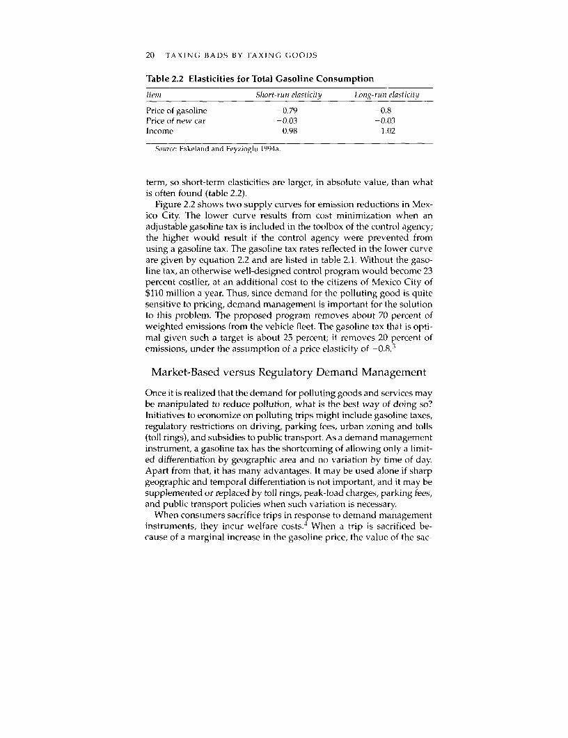
Table 2.2 Elasticities for Total Gasoline Consumption

Itenm Short-run elasticity Long-runii elasticitw

Price of gasoline -0.79 -0.8Price of new car -0.03 -0.03Income 0.98 1.02

SoIrce: Eskeland and Fevzioglu 1994a.

term, so short-term elasticities are larger, in absolute value, than whatis often found (table 2.2).

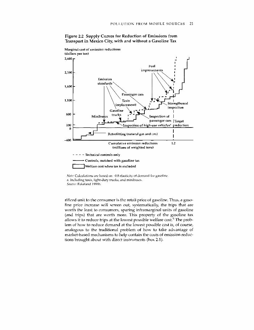
Figure 2.2 shows two supply curves for emission reductions in Mex-ico City. The lower curve results from cost minimization when anadjustable gasoline tax is included in the toolbox of the control agency;the higher would result if the control agency were prevented fromusing a gasoline tax. The gasoline tax rates reflected in the lower curveare given by equation 2.2 and are listed in table 2.1. Without the gaso-line tax, an otherwise well-designed control program would become 23percent costlier, at an additional cost to the citizens of Mexico City of$110 million a year. Thus, since demand for the polluting good is quitesensitive to pricing, demand management is important for the solutionto this problem. The proposed program removes about 70 percent ofweighted emissions from the vehicle fleet. The gasoline tax that is opti-mal given such a target is about 25 percent; it removes 20 percent ofemissions, under the assumption of a price elasticity of -0.8.3

Market-Based versus Regulatory Demand Management

Once it is realized that the demand for polluting goods and services maybe manipulated to reduce pollution, what is the best way of doing so?Initiatives to economize on polluting trips might include gasoline taxes,regulatory restrictions on driving, parking fees, urban zoning and tolls(toll rings), and subsidies to public transport. As a demand managementinstrument, a gasoline tax has the shortcoming of allowing only a limit-ed differentiation by geographic area and no variation by time of day.Apart from that, it has many advantages. It may be used alone if sharpgeographic and temporal differentiation is not important, and it may besupplemented or replaced by toll rings, peak-load charges, parking fees,and public transport policies when such variation is necessary.

When consumers sacrifice trips in response to demand managementinstruments, they incur welfare costs.4 When a trip is sacrificed be-cause of a marginal increase in the gasoline price, the value of the sac-


Figure 2.2 Supply Curves for Reduction of Emissions fromTransport in Mexico City, with and without a Gasoline Tax

Marginal cost of emission reductions(dollars per ton)

2,600 -

Fuel I

2,100 improvements

Emission \stan ards -

1,600-

\\Passenger cars.

1,100 _ Tax'is ,i

\(elceet 1 Srengthened

Gasoline l' I

600 Minibu es trucks n spection of

_ _ passenger cars ITarget

100 Inspection of high-use vehiCleSa freduction

0 ~~~~~~Retrofitting (natural gas and LPG)E

-400Cumulative emission reductions 1.2

(millions of weighted tons)

- - - - Technical controls only

C ontrols, matched with gasoline tax

m Welfare cost when tax is excluded

Note': Calculations are based on -0.8 elasticity of demand for gasoline.a. Including taxis, light-duty trucks, and minibuses.Source: Eskeland 1994b.

rificed unit to the consumer is the retail price of gasoline. Thus, a gaso-line price increase will screen out, systematically, the trips that areworth the least to consumers, sparing inframarginal units of gasoline(and trips) that are worth more. This property of the gasoline taxallows it to reduce trips at the lowest possible welfare cost.5 The prob-lem of how to reduce demand at the lowest possible cost is, of course,analogous to the traditional problem of how to take advantage ofmarket-based mechanisms to help contain the costs of emission reduc-tions brought about with direct instruments (box 2.1).


In Mexico, gasoline is now taxed, but a driving ban is also used inan attempt to curtail driving. The capital's "day without a car" pro-gram, based on the vehicle's license plate number, bans each car fromdriving on a specific workday. Thus the maximal potential effect ondemand that the regulation could have would be to remove 20 percentof workday driving, and the effect would be less if people adjusted inways other than merely canceling trips.

To quantify the costs and benefits of the regulation, one needs toquantify the demand reduction (if any) that it causes and the welfare

Box 2.1 How a Market Can Help

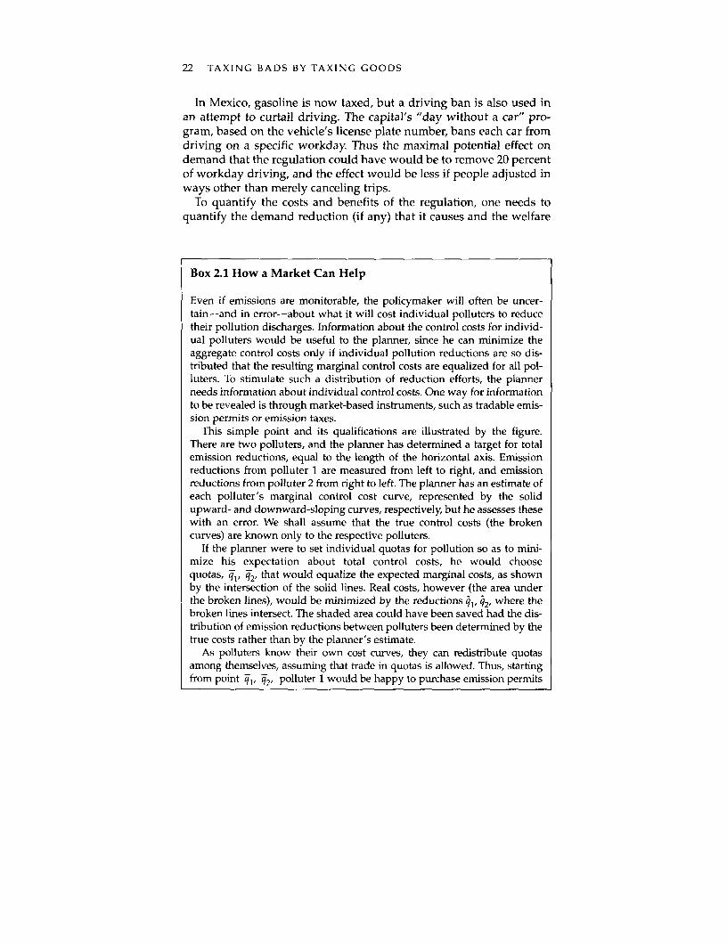
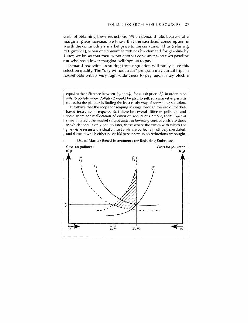
Even if emissions are monitorable, the policymaker will often be uncer-tain-and in error-about what it will cost individual polluters to reducetheir pollution discharges. Information about the control costs for individ-ual polluters would be useful to the planner, since he can minimize theaggregate control costs only if individual pollution reductions are so dis-tributed that the resulting marginal control costs are equalized for all pol-luters. To stimulate such a distribution of reduction efforts, the plannerneeds information about individual control costs. One way for informationto be revealed is through market-based instruments, such as tradable emis-sion permits or emission taxes.

This simple point and its qualifications are illustrated by the figure.There are two polluters, and the planner has determined a target for totalemission reductions, equal to the length of the horizontal axis. Emissionreductions from polluter 1 are measured from left to right, and emissionreductions from polluter 2 from right to left. The planner has an estimate ofeach polluter's marginal control cost curve, represented by the solidupward- and downward-sloping curves, respectively, but he assesses thesewith an error. We shall assume that the true control costs (the brokencurves) are known only to the respective polluters.

If the planner were to set individual quotas for pollution so as to mini-mize his expectation about total control costs, he would choosequotas, q,, i2, that would equalize the expected marginal costs, as shownby the intersection of the solid lines. Real costs, however (the area underthe broken lines), would be minimized by the reductions e1, q2, where thebroken lines intersect. The shaded area could have been saved had the dis-tribution of emission reductions between polluters been determined by thetrue costs rather than by the planner's estimate.

As polluters know their own cost curves, they can redistribute quotasamong themselves, assuming that trade in quotas is allowed. Thus, startingfrom point q,, q2, polluter 1 would be happy to purchase emission permits


costs of obtaining these reductions. When demand falls because of amarginal price increase, we know that the sacrificed consumption isworth the commodity's market price to the consumer. Thus (referringto figure 2.1), when one consumer reduces his demand for gasoline byI liter, we know that there is not another consumer who uses gasolinebut who has a lower marginal willingness to pay.

Demand reductions resulting from regulation will rarely have thisselection quality. The "day without a car" program may curtail trips inhouseholds with a very high willingness to pay, and it may block a

equal to the difference between il, and q2, for a unit price of P, in order to beable to pollute more. Polluter 2 would be glad to sell, so a market in permitscan assist the planner in finding the least costly way of controlling pollution.

It follows that the scope for reaping savings through the use of market-based instruments requires that there be several different polluters andsome room for reallocation of emission reductions among them. Specialcases in which the market cannot assist in lowering control costs are thosein which there is only one polluter, those where the errors with which theplanner assesses individual control costs are perfectly positively correlated,and those in which either no or 100 percent emission reductions are sought.

Use of Market-Based Instruments for Reducing Emissions

Costs for polluter 1 Costs for polluter 2(C1) (C2 )

A AC1 CX,

C2 C

p


household's Tuesday driving, even if the household could more easilyhave sacrificed other trips. Both effects result because the regulationdoes not allow "trading" of the rationed commodity: trips. As shownin figure 2.3, the regulation may curtail inframarginal as well asmarginal trips. The figure illustrates a comparison of a regulatorydemand reduction with a gasoline tax change calibrated to reducedemand by the same amount. The welfare costs of the regulation willbe at least as high, and possibly much higher, depending on the shapeof the demand schedule and the selection of trips that are squeezed outby the regulatory measure. A key assumption in this argument is thatif the regulation achieves any emission reduction at all, it will do sothrough its impact on aggregate gasoline consumption. Then, as weargued above, using market forces to allocate any reduction (in gaso-line consumption, this time, rather than in emissions) will help containthe total costs of the reductions.

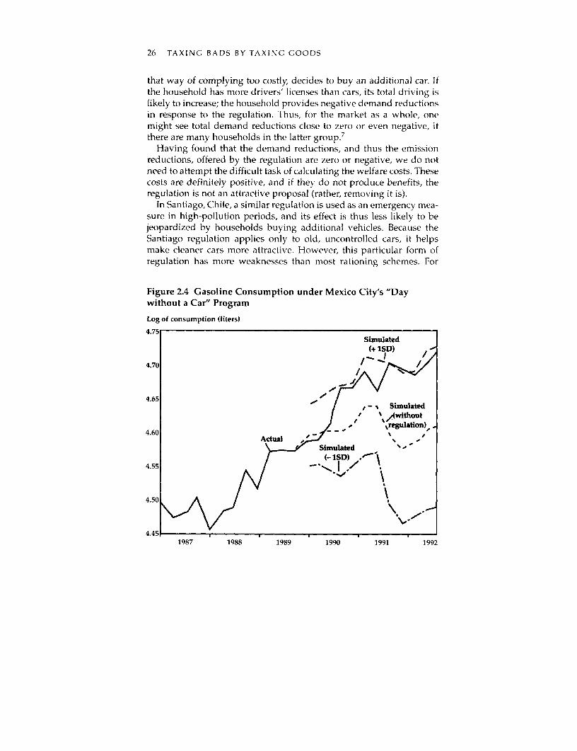
In order to estimate the demand reduction caused by the regulation,a demand function was estimated based on data from Mexico City forthe periods before the regulation (Eskeland and Feyzioglu 1994b).Since the demand function is estimated in periods without regulation,it can be used to simulate counterfactual demand scenarios for subse-quent periods as if no regulation had been implemented. The result,which was indeed surprising, is shown in figure 2.4. One would expectactual consumption to be lower than in the counterfactual simulation,but this occurs only in the first two quarters. After that, actual con-sumption exceeds and stays above the levels forecast by the simulationmodel. 6 Moreover, the indicated confidence intervals (obtained byshifting forecast values up and down by one standard deviation) showthe extremely low probability of observing the actual string of con-sumption levels if demand had not been shifted upward by the regu-lation. (The probability of observing one value outside the confidenceinterval is about 3 percent; observing many is much less likely.) Thuswe can safely conclude that, after an initial period of adjustment, gaso-line consumption was not curtailed by the regulation but rather wasboosted, or at best held constant. (This result is supported by theappropriate Chow test.)

The result is not intuitive, and to try to explain it, one may thinkthrough the ways households can respond to the regulation. Onehousehold complies as expected-by managing without its car onTuesday, sharing rides with friends, using the metro, and postponingor canceling trips. Of course, if the trip is only deferred to another day,total demand reduction would be zero, but otherwise one wouldexpect demand reductions to be positive. Another household, finding


Figure 2.3 Costs of an Increase in the Gasoline Tax versus Regulation

Cost of tax increase

Cost(pesos)

p + t + dt-

p mandnan

iq . q (gasoline consumption, in liters)dq

Welfare cost of driving ban

Cost(pesos)

p +

Heand q i n , t

Li + + % = q (gasoline consumption, in liters)


that way of complying too costly, decides to buy an additional car. Ifthe household has more drivers' licenses than cars, its total driving islikely to increase; the household provides negative demand reductionsin response to the regulation. Thus, for the market as a whole, onemight see total demand reductions close to zero or even negative, ifthere are many households in the latter group.7

Having found that the demand reductions, and thus the emissionreductions, offered by the regulation are zero or negative, we do notneed to attempt the difficult task of calculating the welfare costs. Thesecosts are definitely positive, and if they do not produce benefits, theregulation is not an attractive proposal (rather, removing it is).

In Santiago, Chile, a similar regulation is used as an emergency mea-sure in high-pollution periods, and its effect is thus less likely to bejeopardized by households buying additional vehicles. Because theSantiago regulation applies only to old, uncontrolled cars, it helpsmake cleaner cars more attractive. However, this particular form ofregulation has more weaknesses than most rationing schemes. For

Figure 2.4 Gasoline Consumption under Mexico City's "Daywithout a Car" Program

Log of consumption (liters)

4.75Simulated

(+ ISD)

4.70 I

4.65 o/ -' sSimulated

s R s (/without

4.60 ., regulation),

Simulated

4.55 g/ (-1SD)

4.50

4.451987 1988 1989 1990 1991 1992


example, it allows households to purchase "implicit driving permits"by buying cars, thus tying up the nation's capital unproductively. Inaddition, the limits involved relate to certain trips, rather than to ahousehold's total driving, thereby introducing more limitations thannecessary, even for within-household reallocations. 8

If pollution (or congestion) problems show sharp variations spatiallyor by time of day, demand management instruments such as provisionand subsidization of mass transport, parking policies, and so on may beused to complement the effects of gasoline prices. In transport projects,by contrast, time savings are the main benefits produced. Krupnick(1992) found that the inclusion of emission benefits in the analysis ofprojects designed to reduce congestion and produce time saving is notdifficult in principle and should be done. He also found, however, thatcongestion- and time-saving benefits would probably dwarf pollutionbenefits in such projects. Thus, the inclusion of emission benefits is notlikely to tilt the balance in favor of large investments in transport infra-structure if the projects would otherwise be difficult to justify.

Among the stylized facts cited by Krupnick is that developing coun-try cities with air pollution problems invariably are growing rapidly.Thus he recommends against using modeling frameworks that do notincorporate long-term phenomena such as residential developments.This warning is, of course, relevant if one considers the empirical find-ings of short-term studies, such as the many models of travel modechoice. These studies often conclude that choice of travel moderesponds very little to changes in parameters such as travel costs andtravel times (elasticities usually are between zero and 0.2 in absolutevalue), so that better or cheaper mass transport will do little to reducethe use of private cars. The results from Swait and Eskeland's (1995)mode choice model for Sao Paulo are in line with others from industri-al as well as developing countries. They can be read as a warningagainst the belief that mass transport can perform wonders in curtail-ing private transport. It is important to remember, however, that thesemodels represent household behavior in a very restricted setting. In thelong run, when hlouseholds choose where to live, where to work, howmany cars to own, and so on, behavior may indeed be more sensitiveto gasoline prices, fares, and travel times than these models indicate.

Market-Based and Other Inducementsfor Cleaner Cars and Fuels

We can distinguish between the "physical" changes that can deliveremission reductions (such as a tune-up) and the policy instruments


used to induce those changes. For cars in use, standards and manda-tory inspection and maintenance programs are ordinarily the mostimportant policy instruments. Higher gasoline prices will bring aboutsome additional attention to maintenance and tuning and may evenincrease the market share of smaller cars. However, gasoline priceincreases can only trigger those options that are driven by fuel effi-ciency considerations.

Emission standards and gasoline taxes are indirect instruments: thefirst is a regulation addressing a characteristic of the equipment (thecar's emission factor), the second, a market-based instrument address-ing a proxy for the car's utilization. Emission standards have to bedesigned to stimulate those physical solutions that can cost-effectivelyimprove emissions for the average car.9 Other instruments might trig-ger options attractive only for selected cars. Furthermore, the binarynature of compliance versus noncompliance gives rise to some weak-nesses; cars that are in noncompliance are pushed to become cleaner,but owners of cars in compliance have no incentive to reduce emis-sions, even though some of them might be able to do so cheaply. Sim-ilarly, standards may inadvertently require costly changes for vehiclesthat are close to but not in compliance, even though those changes mayyield very low benefits in comparison with costs.

Could there exist a large number of vehicles in use for which eco-nomic ways of reducing emissions might be devised, when standardsset for the average vehicle do not stimulate these reductions? Clearly,there could. 10 To illustrate, we refer to a feature frequently found in theeconomics of pollution controls: fixed costs. A tune-up, a retrofit witha catalytic converter, and conversion to natural gas all have one thingin common: a fixed cost is paid up front, but emission reductions arerealized as a flow through subsequent periods, proportional to the uti-lization rate and the lifetime of the equipment. Such vehicle modifica-tions are more cost-effective the higher the vehicle's utilization. Thus astandard set to induce measures that are cost-effective for a vehicletraveling the average 8,000 kilometers per year (for Mexico City) willfail to induce many of the control options that are costlier, but morecost-effective, for cars used more intensively

Of course, standards for vehicles in use can be complemented witha wide range of instruments, which could target some of theseoptions directly. However, technical constraints limit how finelythese instruments may be designed. Two possible vehicle modifica-tions-conversion to natural gas and retrofitting with a catalytic con-verter-may serve as illustrations. Conversion gives the owneraccess to a fuel-natural gas-that can be priced independently.


Thus, adjustments in the relative price of natural gas may be used toinduce high-use vehicles to self-select for conversion. A similarscheme to induce retrofitting with a catalytic converter is not feasi-ble; a lower price for unleaded gasoline cannot be used to inducesuch conversions, since unleaded gasoline can be used with or with-out a catalytic converter. Moreover, the prices of leaded and unleadedgasolines may need to be kept close together to avoid encouragingmisfueling, as use of leaded gasoline in a car with a catalytic con-verter poisons the catalytic converter and irreversibly damages itsability to reduce emissions. 11 One could look for other ways of select-ing high-use cars to be retrofitted with catalytic converters-forinstance, by introducing separate requirements for taxis and deliverytrucks. Such classifications of vehicles are surely rough proxies forutilization; taxis in Mexico City travel about nine times the annualaverage mileage for personal vehicles and may thus be useful asbases for indirect instruments, if that is administratively feasible.Since taxis have to have licenses issued by the city, making specialrequirements for them is usually simple.' 2

The important lesson is not that taxis and delivery trucks should becleaner than most cars (although this will often be desirable). Morefundamentally, the absence of comprehensive information based oncontinuous emission monitoring leads the agency to a detailed exami-nation of where and how emissions can be squeezed. The agency thenconsiders the economics of the reductions themselves, under alterna-tive inducement mechanisms. A good agency tries to allow maximumflexibility for polluters, leaving room for solutions it had not imaginedor had thought uneconomic. It may still be the case, however, that sep-arate indirect instruments must be used to stimulate separate groupsof polluters or to pursue separate avenues. In that case, much respon-sibility for analysis rests with the agency.

Effects on Income Distribution

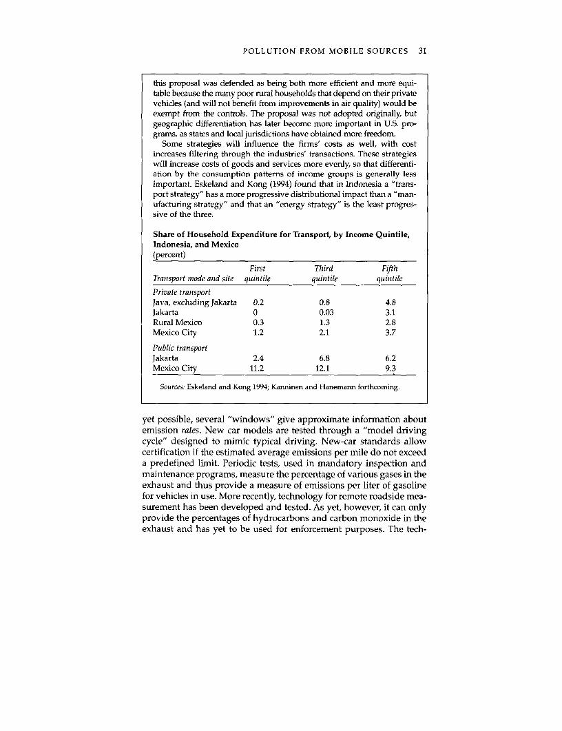
Finally, there is the issue of income distribution effects. Usually, otherpolicies can be found that redistribute income more effectively, andpollution control strategies that minimize total costs can be chosen.However, the analytical issues are not complex, as the cost of controlstrategies generally will be distributed among households accordingto consumption patterns for pollution-intensive goods (box 2.2). Thus,strategies for income-elastic goods-such as private vehicles-will, toa greater extent, be paid for by wealthier households, while strategiesfor necessities will have a less progressive incidence. This will be true


Box 2.2 Distribution of Effects by Income Group

Does concern for income distribution dictate the choice between pollutioncontrol instruments? Before analyzing the income distribution effects of con-trol strategies, one should remember that other instruments may exist that arebetter tailored for redistributive goals than is the modification of pollutioncontrol programs. If so, pollution control programs can focus on efficiency.

A textbook on welfare economics would recommend that a polluter facethe social marginal costs of her choices. Polluters who pay both their owncontrol costs and fees for the remaining emissions will have a self-interestin finding the most effective means of pollution control. This idea-whichis based on efficiency considerations, not equity or other income distribu-tion concerns-has flavored the so-called "polluter-pays principle,"adopted as a policy guideline by the Organisation for Economic Co-operation and Development (OECD 1975) and by many countries. (The OECDformulation specifies that polluters pay for abatement, but it is silent aboutpaying for damages.)

In comparison with an uncontrolled environment, both taxes and regu-lation introduce private costs for polluters, although with taxes, part of thecosts are merely transfers to the government. Under both systems, costs aredistributed among households according to consumption patterns: for apolluting good, the share of the control costs paid by the rich will be higher,the greater is their role in consumption of that good. As the table shows,higher-income households in Jakarta and Mexico City spend a higher shareof their income on their automobiles (counting purchase, maintenance,repairs, and fuels) than do the poor. Thus, policies being paid for byvehicle-owning households will, in general, have a progressive impactacross households (Eskeland and Kong 1994).

Studies of the income distribution effects of control programs in theUnited States in the 1970s yielded some important insights (see Harrison1977). One was the proposal of a "two-car strategy" designed to allow "dirt-ier" cars in areas where air pollution was not a problem. In the United States

whether one chooses regulatory or tax-based strategies, but the dis-tributed costs are higher for tax-based strategies, since these includetransfers to the government. (Then, distributional assessments shouldinclude how the revenues are used.)

Monitoring Technologies and the Needfor Detailed Program Evaluation

Although continuous monitoring of emissions at the source (say, by arunning meter, as for billing water or electricity consumption) is not


this proposal was defended as being both more efficient and more equi-table because the many poor rural households that depend on their privatevehicles (and will not benefit from improvements in air quality) would beexempt from the controls. The proposal was not adopted originally, butgeographic differentiation has later become more important in U.S. pro-grams, as states and local jurisdictions have obtained more freedom.

Some strategies will influence the firms' costs as well, with costincreases filtering through the industries' transactions. These strategieswill increase costs of goods and services more evenly, so that differenti-ation by the consumption patterns of income groups is generally lessimportant. Eskeland and Kong (1994) found that in Indonesia a "trans-port strategy" has a more progressive distributional impact than a "man-ufacturing strategy" and that an "energy strategy" is the least progres-sive of the three.

Share of Household Expenditure for Transport, by Income Quintile,Indonesia, and Mexico(percent)

First Third FifthTransport mode and site quintile quintile quintile

Private transportJava, excluding Jakarta 0.2 0.8 4.8Jakarta 0 0.03 3.1Rural Mexico 0.3 1.3 2.8Mexico City 1.2 2.1 3.7

Public transportJakarta 2.4 6.8 6.2Mexico City 11.2 12.1 9.3

Sources: Eskeland and Kong 1994; Kanninen and Hanemann forthcoming.

yet possible, several "windows" give approximate information aboutemission rates. New car models are tested through a "model drivingcycle" designed to mimic typical driving. New-car standards allowcertification if the estimated average emissions per mile do not exceeda predefined limit. Periodic tests, used in mandatory inspection andmaintenance programs, measure the percentage of various gases in theexhaust and thus provide a measure of emissions per liter of gasolinefor vehicles in use. More recently, technology for remote roadside mea-surement has been developed and tested. As yet, however, it can onlyprovide the percentages of hydrocarbons and carbon monoxide in theexhaust and has yet to be used for enforcement purposes. The tech-


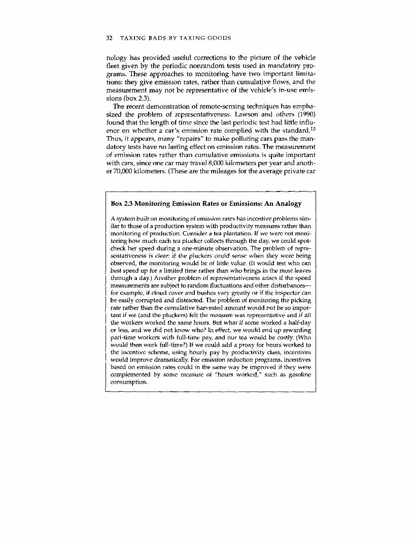
nology has provided useful corrections to the picture of the vehiclefleet given by the periodic nonrandom tests used in mandatory pro-grams. These approaches to monitoring have two important limita-tions: they give emission rates, rather than cumulative flows, and themeasurement may not be representative of the vehicle's in-use emis-sions (box 2.3).

The recent demonstration of remote-sensing techniques has empha-sized the problem of representativeness. Lawson and others (1990)found that the length of time since the last periodic test had little influ-ence on whether a car's emission rate complied with the standard.13Thus, it appears, many "repairs" to make polluting cars pass the man-datory tests have no lasting effect on emission rates. The measurementof emission rates rather than cumulative emissions is quite importantwith cars, since one car may travel 8,000 kilometers per year and anoth-er 70,000 kilometers. (These are the mileages for the average private car

Box 2.3 Monitoring Emission Rates or Emissions: An Analogy

A system built on monitoring of emission rates has incentive problems sim-ilar to those of a production system with productivity measures rather thanmonitoring of production. Consider a tea plantation. If we were not moni-toring how much each tea plucker collects through the day, we could spot-check her speed during a one-minute observation. The problem of repre-sentativeness is clear: if the pluckers could sense when they were beingobserved, the monitoring would be of little value. (It would test who canbest speed up for a limited time rather than who brings in the most leavesthrough a day.) Another problem of representativeness arises if the speedmeasurements are subject to random fluctuations and other disturbances-for example, if cloud cover and bushes vary greatly or if the inspector canbe easily corrupted and distracted. The problem of monitoring the pickingrate rather than the cumulative harvested amount would not be so impor-tant if we (and the pluckers) felt the measure was representative and if allthe workers worked the same hours. But what if some worked a half-dayor less, and we did not know who? In effect, we would end up rewardingpart-time workers with full-time pay, and our tea would be costly. (Whowould then work full-time?) If we could add a proxy for hours worked tothe incentive scheme, using hourly pay by productivity class, incentiveswould improve dramatically. For emission reduction programs, incentivesbased on emission rates could in the same way be improved if they werecomplemented by some measure of "hours worked," such as gasolineconsumption.


and the average taxi, respectively, in Mexico City.) Measuring only theiremission rates leads to equal incentives to clean up both, although thesocial returns from reducing emission rates differ by a factor of nine.

Periodic tests and the institutional and technical systems that sup-port them are improving, reducing the scope for both poor measure-ment and weaknesses due to corruption.1 4 The representativeness ofthe tests is being gradually improved through better technology andmore resources (loaded mode tests, longer-cycle tests, and closer vehi-cle inspection). Other, but less likely, developments that could improverepresentativeness are surprise roadside tests and a technology forreading cumulative emissions since the last test.15

Given present monitoring capacity, an obvious way to improve theapplied systems would be to read the emission rate from the car'sannual test, multiply it by the cumulative mileage (on a tamperproofodometer), and apply an emission fee based on the result. The feecould be paid on testing, or it could be paid uniformly at the gas sta-tion as a presumptive tax, to be refunded in part to owners of vehiclesfound to be "cleaner" than was presumed in the prepaid tax.

The efficiency gains from such a reform would come through severalchannels. First, all owners would have continuous incentives to driveless, and owners of more polluting cars would, appropriately, havemore of those incentives than others. Second, all owners would haveincentives to make their cars cleaner, but owners who use their carsrarely would feel less of this pressure than owners with higher mileage.As a consequence, society would waste few resources cleaning or scrap-ping cars that are rarely used. Third, the car market would facilitateexchange of vehicles, to make sure that households and firms which usetheir vehicles intensively would end up with the cleaner ones.

Notes

1. This perspective is examined in detail in Eskeland (1994b), from whichmuch of this material is selected. We use the term gasoline tax, but the sameprinciples apply to other polluting inputs, such as diesel fuel.

2. Detailed calculations are shown in Eskeland (1994b). An important pointis that income is here valued equally whether it accrues to the public sector orto private households. This treatment therefore abstracts from income distri-bution effects and revenue effects.

3. In Mexico City alone such a gasoline tax would collect between $300 mil-lion and $350 million in tax revenues annually. A gasoline tax motivated bypollution control objectives should, ideally, be higher in urban areas, but thegeographic differences may have to be limited for administrative reasons.Gasoline may also be taxed for general revenue and other purposes, of course.

4. We use trips and gasoline as metaphors for polluting goods and inputs.


Consequently, if gasoline is saved by using more fuel-efficient cars, the argu-ment applies as if trips were saved. Other fuels should be taxed according toemissions, as well.

5. When calculating the welfare costs of manipulating consumption, weneed to emphasize that we employ the "compensation criterion": we assumeno value (or penalty) associated with the transfer of money from private topublic hands, or from poor to rich. Thus the analysis ignores any concern forincome distribution, as would be correct if transfers could be arranged cost-lessly with the use of other policy instruments.

6. Simulations are performed with actual price and income developmentsinserted in the estimated demand model. In all calculations, seasonality andstationarity are taken into account.

7. There is anecdotal evidence that many households bought used cars; thatis, Mexico City imported old cars from the rest of the country. If this did hap-pen, use may have shifted toward cars that are dirtier per liter than the aver-age car, which would make the consequences for emissions worse than indi-cated by aggregate consumption.

8. Rationing nontradables in this case, trips-thus has higher welfare coststhan rationing tradables with low resale costs, such as, say, alcohol and tobacco.

9. Regulations, or their enforcement, can allow for some differentiation,which may be desirable for efficiency or equity reasons. For instance, regula-tions might be applied only in polluted areas (see Harrison 1977, an earlystatement of this point) or to certain model years, weight classes, and so on.Cars that cannot pass the emission test in Mexico City could be used in otherareas of the country-a very desirable feature in a poor country where ambi-ent air pollution is the least of the problems in rural villages.

10. Anderson (1990) provides an interesting practical review of strategiesapplied to reduce emissions from in-use vehicles. McConnell and Harrington(1992, 1993) evaluated strategies for detecting high-emitting vehicles. Theyfound that the continued presence of such vehicles, despite standards andscheduled testing, is due partly to monitoring problems but also to caps allow-ing a vehicle to operate when a specified tune-up cost has been incurred.

The efficiency of programs to make cars and fuels cleaner depends on howwell they screen vehicles with respect to relevant parameters. As an example,Alberini, Harrington, and McConnell (1993) analyzed a buyback programdesigned to get cars with higher emissions off the streets. They found that theprogram selected for some desirable characteristics (poor operating condition)but also for some undesirable ones (low expected remaining lifetime mileage).Krupnick, Walls, and Collins (1993) compared various instruments, includinga corporate average fuel economy (CAFE) standard. They found that a tougherCAFE standard was not cost-effective, even if the emission control objective inquestion was for greenhouse gases.

11. Measures that discourage misfueling (such as nozzle-size regulations,enforcement, and octane differences) can easily fail if the price differencebetween leaded and unleaded gasoline is large.

12. For example, the "tier 1 standard" yields emission reductions at a cost of$322 per ton for taxis in Mexico City and $1,629 per ton for other cars (see table2.1).

13. Harrington and McConnell (1993) find that the use of remote (and thusunscheduled) sensing techniques is cost-effective in comparison with man-


dated periodic testing under plausible assumptions. It would also provideadditional emission reductions cost-effectively in areas with establishedinspection and maintenance programs.

14. For instance, computerized testing equipment may print automaticallya certification sticker based on the test result. Such advances may be of littlehelp, however, if random or other disturbances allow the gas sensor to be heldaway from the tailpipe.

15. Of course, the development of such a technology could be stimulated byoffering car owners a rebate on the gasoline tax based on the reading of theircumulative emission meter (it would have some interesting incentive effects).

Other illustrations of monitoring techniques and problems may be cited. InMexico City surprise roadside tests were, perhaps laudably, resisted as anenforcement measure. It was felt that the public should be spared police inter-ruption unless on specific suspicion. In Jakarta policemen have been autho-rized to fine smoking vehicles on the basis of visual assessment. In LosAngeles the public may call authorities to report smoking buses.

3. Control of Pollutionfrom Industrial Sources

Perhaps the most important feature distinguishing industrial pollutersfrom vehicles is the much greater heterogeneity of the former.Although motor vehicles certainly differ in important respects (age,size, fuel, combustion and emission control systems, maintenance, andutilization), they may easily be placed in a small number of categories.In each category-new personal gasoline vehicles and used personalgasoline vehicles, for example-there will be a high number of pol-luters that are reasonably homogenous (almost all use an internal com-bustion engine to produce transport services), and we can know eachgroup reasonably well by sampling a small subset.

Industrial sources are necessarily more heterogeneous. Cars primar-ily pollute the air, while firms pollute all media, and with a widerrange of pollutants. Firms' technologies, equipment, and use of inputsvary much more, mainly because of their more varied outputs. Thus, apriori, it would appear more dangerous for the planner to assume heknows the emission control opportunities open to firms than it wouldbe in the case of vehicles.

Another important difference is that firms' quantitative impact variesmnuch more, so that a few sources may dominate as contributors to a pol-lution problem. In Java two pulp factories represent 37 percent of indus-trial discharges (measured as biological oxygen demand) in one river,and two other factories account for 92 percent in another stream.According to a registry of the ninety largest polluters in the Valley ofMexico, two firms emit 95 percent of total dust emissions, and 10 per-cent of firms emit 99.5 percent. By contrast, even the most polluting ofvehicles will-individually-play only a minor role. Even if oneselected the most-polluting vehicles in Mexico City, more than 100,000vehicles would be needed to account for 50 percent of total emissions.

These two features distinguishing industrial polluters, or fixed-pointsources as they are often called in the literature, have implications for

36

CONTROL OF POLLUTION FROM INDUSTRIAL SOURCES 37

pollution control policy. The greater heterogeneity of sources meansthat the planner will have a weak basis for assessing individual emis-sions and control options. Thus, if the planner tried, through samplingand a rough categorization of polluters, to make prescriptions foreach-in terms of allowable emissions or of abatement technologies tobe applied-it would be on the basis of grossly inadequate information.The resulting emission reduction would, consequently, come at a highcost. By contrast, the greater dominance of a few polluters makes it eas-ier to devise strategies for cost-effective emission reduction. The plan-ner might, for instance, commission engineering studies of a firm's or asector's emissions and control opportunities and so bridge part of theknowledge gap between the sector and himself.

In industrial as well as developing countries, pollution control agen-cies issue standards for industrial pollution control whereby a firm's"allowable" emissions or practices are determined on the basis ofrough categories (such as "textiles," as reported by the firm). Stan-dards and regulation in developing countries are, at best, determinedon the basis of a study that has sampled a few firms in the category.More often, the standards are based not on local studies but on studiesfrom other countries, without much questioning of their adequacy orrelevance for local conditions. Also, plant-specific studies may be doneon large polluters, attempting to take into account factory-specific andrecipient-specific conditions. Such studies then form the basis forplant-specific regulation, allowable time for attaining compliance, andso on. Thus there is ample evidence that the agency recognizes thecosts associated with the information gap. We argue in this chapterthat policy instruments are available for dealing with such problemsbut that their full potential is not exploited.

General Economic Policies, Inputand Output Taxes, and Regulation

If the planner, or society, has an interest in total emissions but lacksinformation about individual emissions, he will inevitably find him-self seeking proxies not only for individual emissions but also forabatement opportunities and costs.1 Thus he is immediately taken faraway from a situation with full information, in which he wouldinclude only information on individual emissions, or damages, in theincentives scheme with which he confronts polluters. In the case ofvehicles (chapter 2), the planner conducted a study to learn about thedeterminants of emissions before deciding to work with manufactur-


ers to encourage production of cleaner vehicles, to intervene in fuelmarkets to tax fuels and make them cleaner, and to use periodic test-ing to encourage proper maintenance and use. Similarly, for firms theplanner needs to have an idea about how emissions are generated inorder to know where and how to squeeze emissions.

Kopp (1992) describes the planner as needing an expanded-although traditional-model of the firm. He includes residuals amongthe variables for which demand and supply functions are specified. Asan example, if the expanded model shows that emissions are highlysensitive to the characteristics of a firm's capital equipment, equipmentcould be a useful point of intervention-and monitoring-in the incen-tive scheme. Similarly, should the expanded elasticity matrix indicatethat emissions-say, of sulfur-are sensitive to the relative prices of sul-fur-rich fuels, taxation of these could provide emission reductions in away that greatly economizes on monitoring and enforcement.

Economic studies of pollution often use quite superficial models ofemission generation. For instance, marginal emission factors may beassumed to be fixed by sector according to either output or fuel use,abstracting from much of the variation among plants in characteristicsand behavior. They will therefore be inadequate for analyzing policiesaimed at modifying the determinants of emission factors at the firmlevel. By contrast, such models have credibility in analysis of policiesthat would mainly change incentives at broader levels. In the case ofoutput-based emission factors by sector, the models are adequate forsimulating the effects of sector-specific taxes, trade policy, and indus-trial policy. In the case of emission factors linked to fuel use, the mod-els may also simulate well the effects of energy-pricing policy and con-servation initiatives.

A major research effort in the World Bank (Hettige and others 1995)has estimated sector-specific emission coefficients on the basis of U.S.manufacturing data. Using such emission coefficients, Ten Kate (1993)studied how industrial pollution had developed in Mexico in theperiod 1950 to 1989. Growth in manufacturing over the period wasremarkable-a tenfold increase in output. But Ten Kate observed thatpollution had increased also because of an uninterrupted change inoutput composition, increasing the share of the more-polluting sectors.Surprisingly, Ten Kate found no breaks in this trend that could be asso-ciated with the distinct changes in economic policy over the years,from an emphasis on import substitution, through the period domi-nated by rising petroleum revenues and public sector expansion, tostabilization and liberalization in the 1980s. He found evidence thatMexico, through low domestic energy pricing, had "escaped" the envi-


ronmental benefits associated with rising world energy prices after1973. Mexican industry increased its average energy intensity by 6 per-cent from 1970 through 1990, a period in which OECD countriesreduced their average energy intensity by 38 percent. Apart from thisobservation, Ten Kate found that rapid expansion in a few highly pol-luting sectors, such as agro- and petrochemicals, drove much of theincrease in average emission coefficients. Since those are sectors withpredominant public sector influence, and domestic energy pricing hasrelied on public subsidies (equivalent to 4-7 percent of gross domesticproduct, or GDP ), Ten Kate left open the possibility that domestic pol-icy had a major influence on the increased emissions.

Energy Conservation and Interfuel Substitution

While the differences between sectors in terms of their emission inten-sities are important, it is highly desirable to provide more sophisticatedincentives in order to induce responses along a greater range of possi-bilities than simply varying sectoral output levels.2 One way of doingthat, short of monitoring emissions from each firm, is to exploit thelink to energy use, which is particularly strong for air pollution.

For industrial as well as for other polluting activities, it is cost-effective to pursue emission reductions through technical controls, aswell as through demand reductions. The marginal costs of emissionreductions through these two means will be equalized if emissiontaxes (or tradable permits) are used. Otherwise, presumptive taxes onpolluting goods should be used, complementing mandated technicalcontrols to equalize marginal costs. Cost-effective programs (and,among these, optimal programs) are characterized by tax levels on pol-luting goods (t) which, when normalized by marginal emission coef-ficients (e'), equal marginal costs of emission reductions through tech-nical controls: tl/e. = c,. The formula emphasizes that a polluting goodshould be taxed in proportion to its emission coefficient as long asemissions themselves are not taxed.

For firms, we shall not here develop technical control cost curves, aswe did for automobiles. We shall, however, investigate the scope for"purchasing" emission reductions via taxation of a particularly impor-tant category of polluting goods-fuels-using a rather simple modelof how air pollution emissions from manufacturing respond to pricechanges:3

(3.1) tdpl ,, ax,, all];)a'( -


where et, is emissions of pollutant mi, summation is over a set of inputscategorized as polluting (fuels), 'e,Z,/dxi(W) is the marginal emissioncoefficient for fuel i when a, characterizes the technology, and axi/apj isthe price responsiveness of demand of fuel i with respect to a price p,.We thus turn to the topic of emission coefficients and demand elastic-ities for fuels in manufacturing.

On the link between fuel use and emissions, it is worth noting thatthe technically based literature (summarized, for instance in u.s. EPA

1986) usually projects emissions by constant emission factors, specifiedin grams of pollutant per unit of fuel. These will generally vary bymeasurement, in part according to identified characteristics (for burn-ers, according to configuration and firing conditions; for coal, accord-ing to ash content, and so on) but will be averaged when applied to apopulation of polluting sources.4

The use of fuel consumption as the basis for emission models hastraditionally been motivated mostly by technical reasoning. Experi-ence about emission rates from different types of equipment and pro-cesses is then based on sample testing or theory, and fuel throughputmay be viewed as a proxy for the utilization of the equipment. Analternative check, to our knowledge previously untried, is to regressreported emission intensities against information on energy use andother possible determinants. For PM-10 (small dust particles),arguably the air pollutant of greatest concern in many developingcountries (see Ostro 1994), the energy cost share is highly significant,with a positive sign, in explaining variations in emission intensities.5

This holds whether or not other variables, such as dummies for theStandard Industrial Classification (sic) industry code, cost shares formaterial inputs, and the like, are included among the explanatory vari-ables. Moreover, many sic industry dummies that are not significant inexplaining variations in PM-10 emission intensities when the energycost share is not included in the model are significant when energy isincluded. Those industries can be said to represent "clusters" in termsof PM-10 emission intensities, but only if the variation due to differ-ences in energy intensity is taken into account. A similar test has yet tobe performed using data on different types of fuel as the explanatoryvariables, since such data have not been merged with emission data.

Given that different fuels pollute differently, the scope for interfuelsubstitution and energy conservation will be an important determinantof the effectiveness with which fuel taxes can be used to reduce emis-sions. To estimate the substitutability of different fuels, we have resortedto both econometric and engineering studies. Econometric studies donot provide information on emissions and often require abstractions


where specificity would be desirable for the purposes of this study.(See, for example, Kopp 1992 on the eclectic use of estimates based part-ly on econometric studies, partly on technical studies and expertise.)

The experience of the OECD countries since the 1973 oil price shockindicates that the possibilities for energy conservation and interfuelsubstitution are quite high. Between 1971 and 1988 manufacturing out-put in OECD countries rose 62 percent, while energy use (measured intons of oil equivalent, or TOE) remained unchanged, implying a 38 per-cent reduction in average energy intensity (Bacon 1992). By contrast, inMexico, where energy prices were suppressed domestically, the ener-gy intensity of manufacturing increased during the same period (TenKate 1993). Using separability assumptions and flexible functionalforms, Fuss (1977) and Pindyck (1979) estimated own-price elasticitiesfor individual fuels in manufacturing to be in the range -0.7 to -2.2.Own-price elasticities for aggregate energy were estimated at -0.5 byFuss and -0.7 by Pindyck. The whole set of own- and cross-price elas-ticities is relevant for the responsiveness of emissions of each pollutantto a specific fuel price, but the price elasticity for aggregate energy hasa more immediate interpretation: a price elasticity for aggregate ener-gy of 0.5 implies that an equiproportionate price increase of 20 percentfor all fuels (and electricity) would reduce demand for all fuels by 10percent and, consequently, emissions of all pollutants by 10 percent. 6

The evidence from developing countries has been more limited. Animportant study on Indonesian manufacturing (Pitt 1985) used plant-level data over three years (1976-78). Pitt estimated the own-price elas-ticity for aggregate energy to be between -0.1 and -0.8, overlappingthe Fuss-Pindyck range. He was able to estimate models that distin-guished between subsectors of manufacturing, and, in general, hefound higher elasticities for the more energy-intensive sectors.

Moss and Tybout (1994) studied how much of the change in theenergy intensity of manufacturing in Chile has been due to shifts inoutput levels among subsectors and how much to changes in input useat the plant level. They concluded, perhaps surprisingly, that much ofthe change has come from shifts in input use at the plant level. This isan important finding, since many econometric studies based on aggre-gation over firms and sectors are unable to distinguish flexibility with-in firms and sectors from shifts between energy-intensive sectors andother sectors. A subsequent study (Guo and Tybout 1994) estimatedinterfuel substitutability for selected subsectors on the basis of firm-level observations and found that there is considerable substitutabilitybut that it varies by subsectors and across plants. (The estimates arealso sensitive to the choice of model for estimation.)


Eskeland, Jimenez, and Liu (1994) estimated, for manufacturing,own- and cross-price elasticities for different fuels in Chile andIndonesia, with a view toward assessing the potential of fuel taxes forreducing emissions. A model with separability between an energyaggregate and other inputs yields various results, depending on theassumed policy experiment. (The methodology follows that of Fuss1977.) One possibility is to assume that aggregate energy is held con-stant; another is to assume that output is constant but that substi-tutability between energy, materials, and labor occurs. When aggre-gate energy is held constant (the "energy submodel"), the relativeprice of one energy source (a fuel, or electricity) is increased, while theprice and use of aggregate energy is constant. When only output isconstant, the price of the energy aggregate changes when an individu-al fuel price changes. For Chile the authors report on estimates basedon both assumptions, while for Indonesia only the energy submodelcould be estimated.

Table 3.1 presents estimates of Chilean price elasticities of demandfor the first case, in which aggregate energy is held constant. The sixenergy sources in the original study have been aggregated into three toprovide a simpler display of policy tools. Note that all the own-priceelasticities are negative and are fairly large in absolute value. At sucha general level, the results are in line with earlier research (for instance,Pindyck 1979). In the full elasticity matrix, twenty-four of the thirty-sixelasticity estimates are significantly different from zero at the 5 percentlevel and an additional two at the 10 percent level. The fossil fuels aresorted according to the intensity of their TSP (total suspended particles,or "dust") emissions, with coal, fuel oil, and "grouped fuels" (the lat-ter includes wood and coke) comprising heavy fuels, while diesel andnatural gas comprise light fuels. The elasticities in table 3.1 are calcu-

Table 3.1 Energy Group Elasticities, with Energy Constant, Chile

Price of Price of Price ofDeOiaind electricityl heavy ftuels light fite/s

For electricity -0.98 0.77 0.22For heavy fuels 0.61 -0.89 0.28For light fuels 0.20 0.53 -0.74

Note: Heavy fuels are coal, fuel oil, and grouped fuels; light fuels are natural gas anddiesel. Elasticities are combinations of elasticity estimates in a six-fulel matrix. Most ofthe elasticities are significant at a 5 percent level.

Souurce: Eskeland, Jimenez, and Liu 1994.


Table 3.2 Emission Elasticities, with Energy Constant, Chile

Price of Price of Price ofEmissiotns electricitv heavy fuels liglht Jiels

Electricitv, pollutingSOx 0.07 -0.19 0.11TSP -0.14 -0.09 0.24

Electricity, non polluitingSOx 0.50 -0.58 0.07TSP 0.48 -0.73 0.25

Souirce: Eskeland, Jimenez, and Liu 1994.

lated under the assumption that prices for various fuels in a groupincrease proportionally. 7 As an example, if prices for heavy fuelsincrease by 10 percent, demand for electricity and light fuels willincrease by 7.7 and 5.3 percent, respectively, while demand for heavyfuels will fall by 8.9 percent.

What are the implications of these elasticities for the responsivenessof emissions to price changes? The answer depends to a great extent onwhat happens in the electricity sector, and there are good reasons fortreating that sector separately. First, the electricity sector is reasonablyeasy to sujbject to separate policy instruments, including those based onemission monitoring. Second, since electric power plants may consist inpart of tall-stack units located far away from the most polluted and pop-ulated areas, emissions from the sector should perhaps not be treated inthe same way as emissions generated directly in the manufacturing sec-tor (as each power plant could be treated separately). Table 3.2, for thesereasons, provides emission elasticities under alternative assumptions.The assumption "electricity, polluting" assumes that electricity at themargin is produced 50 percent by coal-fired, uncontrolled plants and 50percent by nonpolluting technologies. The alternative assumption isthat the electric power sector is nonpolluting at the margin.

Again using a 10 percent increase in prices for heavy fuels as anexample, SOx emissions would be reduced by 5.8 percent and TSP

emissions by 7.3 percent under the assumption that the electricity sec-tor is nonpolluting at the margin. Price increases for light fuels would,as expected, increase emissions under all assumptions, since theywould lead to substitution toward more-polluting energy sources.Increases in electricity tariffs would increase emissions significantly ifelectricity is assumed to be nonpolluting. If electricity is assumed to bepolluting at the margin, the tariff increases would lead to a small


increase in SOx emissions and to a small reduction in TSP emissions. Tosum up, price increases for heavy fuels are quite powerful in reducingemissions if and only if the electricity sector is nonpolluting at the mar-gin. The reason, as can be seen in table 3.1, is that much of the induceddemand response is toward electricity.

Table 3.3 shows the calculated group demand elasticities for Indone-sia. In comparison with those for Chile, there are differences, but neg-ative own-price elasticities and positive or small cross-price elasticitiesagain dominate. The own-price elasticity for heavy fuels is larger inabsolute value, making tax instruments more powerful.

Emission elasticities are given in table 3.4. As in the case of Chile,price increases for heavy fuels reduce emissions for both SOx and TSP,

but the magnitudes of the effects are greater for Indonesia. Referringback to tables 3.1 and 3.3, one sees that Indonesia has a higher own-price elasticity for heavy fuels (in absolute value) and a smaller cross-price elasticity with electricity. Thus, emissions respond more to anincrease in prices of heavy fuels. Under the assumption that the elec-tricity sector is nonpolluting at the margin, emission elasticities withrespect to the price of heavy fuels are -1.02 for SOx and -1.52 for rsr.Even under the assumption that electricity is polluting, emission elas-ticities with respect to the prices of heavy fuels for Indonesian manu-facturing are quite large, in the range of -0.8 for SOx and TSP.

These estimates are based on the assumption that the price of theaggregate "bundle" of energy does not change when a fuel price rises.8

However, unless compensatory price changes are made for other fuels,firms will also alter their use of aggregate energy by substituting laborand materials (still holding output constant). For Chile the necessarydeflators for outputs and other inputs could be constructed, and ashort-run model with three aggregate inputs-energy, labor, and mate-rial-could be estimated.

Table 3.3 Energy Group Price Elasticities, with Energy Constant,Indonesia

Price of Price of Price ofDemntid electricityI lcavy ftietls lighti fiels

For electricity -1.02 0.26 0.76For heavy fuels 0.24 -1.41 1.17For light fuels -0.01 0.37 --0.35

Note: See notes to table 3.1.Source: Eskeland, Jimnenez, and Liu 1994.


Table 3.4 Emission Elasticities, with Energy Constant, Indonesia

Price of Price of Price, ofEmfissions lehctricity iheazy filel; light fuels

ElectricitY/, pol0ltingSOx 0.02 0.81 0.79rsp -0.21 -0.86 1.07

Electricit., nionpollutingSOx 0.22 -1.02 0.80TSP 0.26 -1.52 1.25

Source: Eskeland, Timnenez. and LiLl 1994.

Table 3.5 displays the own- and cross-price elasticities in this aggre-gate model. The own-price elasticity of aggregate energy is consider-able, at 0.63, between Pindyck's 0.7 and Fuss's 0.5. This indicates thatdemand for all fuels-and emissions of all air pollutants-would fallby 6.3 percent if all energy prices increased by 10 percent. We may alsonotice that the cross-price elasticity between energy and labor is posi-tive and substantial, indicating that subsidies to energy would be apoor strategy if increased employment were a policy objective.

With aggregate energy adjusting, price elasticities for individualfuels will be modified-own-price elasticities are higher in absolutevalue, while cross-price elasticities are somewhat dampened and may

Table 3.5 Manufacturing: Elasticities for Aggregate Inputs, Chile

Aggregate Pricet o'fenergy mlaterial

DePatnid price Wage inpluts

For energy -0.63 1.57 -(1.95(0.36) (0.49) (0.31)

For labor 0.52 -1.89 1.37(0.16) (0.34) (0.30)

For materials -0.07 0.32 -0.25(0.02) (0.07) (0.08)

Note: Figures in parentheses are standard errors. All coefficients are significant at the5 percent level.

Souirce: Eskeland, Jimenez, and LiLl 1994.


Table 3.6 Emission Elasticities, with Energy Adjusting, Chile

Priec Price of Price of Allof- leaz!vy light enerrg

Et?fissionis electricity fuiels fuels prices

EleXctricitly, polilittitigSOx -0.15 -0.52 0.04 --0.63Tsp -0.37 -0.42 0.16 -0.63

ElectricitYl, nlolpolluting

SOx 0.28 -(.91 -0.01 -0.63TSP 0.25 -1.06 0.18 -0.63

Source: Eskeland, Jimenez, and Liu 1994.

switch sign if they are positive in the energy submodel. The intuitionis that it is easier to change demand for a taxed fuel when one can varythe use of other (nonenergy) factors as well. Energy substitution alsoreduces the tendency for demand to spill over to other fuels. Theimplications for policy are seen in the emission elasticities in table 3.6.The greater own-price elasticities and the lower cross-price elasticitiesincrease the elasticities of emissions with respect to the price of heavyfuels. Under these assumptions, a tax increase for heavy fuels can be apotent instrument for pollution control, whether or not electricity ispolluting at the margin.

Exploration of General Equilibrium Effects

Up to now, we have been discussing the effects of fuel taxes on emis-sions in a partial equilibrium context. For transport, we emphasized therole fuel taxes could play in reducing output in the polluting activity,while other instruments could be used to make each "polluting plant"less polluting per unit of output. In the applications to industrial emis-sions, by contrast, the emphasis has been on the extent to which thesame amount of aggregate output from manufacturing can be deliveredwith less use of energy, or with the use of less-polluting types of ener-gy. In this section we extend these explanations with a computable gen-eral equilibrium (CGE) model of the Indonesian economy.

Increased input taxes, if uncompensated, will alter output levels,since they change production costs. In the case of a fuel tax, fuel-intensive producers and sectors will initially experience the greatestincrease in costs and will thus be under more pressure either to changetheir input mix or to raise output prices. The latter will occur to a great

CONTROL OF l'OLLUTION FROM INDUSTRIAL SOURCES 47

extent if fuel-intensive producers have little flexibility in input choice,and one would expect to see reduced equilibrium output levels in fuel-intensive sectors. The new equilibrium, with a different output combi-nation and different emission levels, will reflect the opportunities forchange open to all agents in the economy.

The CGE model of the Indonesian economy is designed to highlightthe features that are important for energy use (Devarajan and Lewis1994). In particular, the model distinguishes among three types of pri-mary energy (oil, gas, and coal) and three energy products (electricity,gas, and refined oil products) and incorporates the existing system oftaxes and subsidies in the economy. The rest of the model is a fairlystandard CC;E model, with twenty-six productive sectors, four house-holds, five labor groups, and fixed, sector-specific capital.

The model enables us to go deeper than the rather abstract "aggre-gate manufacturing output" discussed above. Table 3.7 shows thegreater degree of specificity in terms of outputs. Eight sectors consti-tute manufacturing in a traditional sense, while six "sectors" convertpetroleum resources to refined products and liquefied natural gas(LNG). Four sectors are engaged in extraction of natural resources, andtwo sectors represent agricultural activities. The first column showsemissions of TSP from each sector, as modeled on the basis of fuel use.In manufacturing, three sectors stand out: chemicals and fertilizer,nonmetallic minerals, and basic metals. Importantly, two "miscella-neous" sectors (electricity and transport) are the two largest in termsof TSP emissions, while construction ranks equally with a manufactur-ing sector such as food processing. The second column shows thedirect emission coefficients, or total emissions from the sector dividedby the sector's gross output.

The CGE model allows us to evaluate the importance of intermediatedeliveries between sectors. The third column presents the sum of thedirect and indirect emission coefficients. That is, it includes not just thedirect effect on emissions of increasing output in a sector by one unitbut also the effects of the interindustry demand stimulated by thisincrease in output. These are important when looking at the economywith a blunt planning perspective. The column informs us, for instance,that an expansion of a sector such as metal products and machinerywould increase output from polluting sectors and thus increase pollu-tion, even though the sector itself does not have a very high emissioncoefficient. This may be relevant if major industrial expansion plans areconsidered and adequate policy instruments are riot in place to influ-ence the levels of pollution directly. If polluting suppliers to the indus-try in question face appropriate tax levels, however, expansion plans


Table 3.7 TSP Emissions by Sector in the Computable GeneralEquilibrium Model, Indonesia

Tonaleni issionis

(tolls Direct Totnl CGESector per yJear) coefficient coefficient coefficient

ManuiifactuiringFood processing 44.7 0.003 0.015 - 0.006Textiles and leather 9.8 0.003 0.039 0.003Wood and furniture 10.2 0.004 0.024 - 0.012Paper and related

industries 3.5 0.003 0.042 -0.002Chemicals and fertilizer 157.5 0.041 0.095 0.016Nonmetallic minerals 220.0 0.136 0.200 0.076Basic metals 164.5 0.090 0.166 0.028Metal products and

machinery 14.8 0.002 0.056 0.002

RefininlgGasoline 0.1 0.000 0.013 -0.095High-speed diesel 0.1 0.000 0.013 -0.017Industria] diesel 0.0 0.000 0.013 -0.211Kerosene 0.1 0.000 0.013 -0.171Fuel oil 0.1 0.000 0.013 -0.570LNG 2.8 0.001 0.004 -0.003

Agricuiltutre anid tnatural resourcesFood agriculture 0.9 0.000 0.007 -0.010Traded agricultlre 4.1 0.000 0.010 -0.010Oil extraction 6.4 0.001 0.004 - 0.000Natural gas 1.1 0.001 0.004 -0.017Coal mining 39.1 0.515 0.603 3.484Other mining 5.5 0.004 0.003 - 0.020

MiscellanIeoUsElectricity and gas 1,668.9 0.999 1.225 0.586Water supplv 0.2 0.002 0.058 0.006Construiction 42.2 0.002 0.043 -0.005Transport 692.2 0.073 0.088 0.020Trade and storage 5.0 0.000 0.015 -0.007Services 6.0 0.000 0.025 0.(

Total 3,037.3Soiirce: Lewis 1994.


for a downstream industry need only pass the test of paying for theeffects of its own emissions (that is, according to direct coefficients).

The calculation of the total coefficient in the third column assumesimplicitly that resources for expanding output are available in perfect-ly elastic supply in this economy. This is why all the total coefficientsare larger than the direct coefficients. In reality, however, when a sectorexpands output, it draws resources from other sectors by bidding upfactor prices. As a result, some other sectors will contract, and the over-all effect on pollution may be positive or negative. The fifth column dis-plays this overall effect when these resource limitations are broughtinto the picture.9 Note that some of the coefficients are negative becausethe higher factor costs resulting from the output expansion in the sec-tor concerned lead to a contraction in more-polluting sectors. In partic-ular, some of the petroleum product sectors-such as kerosene andindustrial diesel-actually have a negative coefficient because anincrease in their output crowds out other, more polluting products.

In general, of course, taxing the polluting activities themselvesaccording to their pollution and damage levels is a good idea. In thecase of fossil fuels, since pollution is related to the use of these fuels (tothe outputs from the refining sectors, strictly speaking), taxation offuels will be a tax on polluters and will have much of the desired effectin terms of inducing using sectors (and users of using sectors' outputs)to reduce polluting inputs.

We turn, therefore, to the impact of changes in tax rates on energyuse and emissions. What would be the effect of eliminating the com-plex system of taxes and subsidies in Indonesia's energy sector? Theanswer, not reported here in detail, is that emissions of most pollutantswould increase. The main reason is that many of the less-pollutingfuels are subsidized at the outset (kerosene and tvo types of diesel, inparticular), and some of the heavier fuels are taxed. Thus, eliminationof taxes and subsidies makes the more-polluting fuels more attractive,contributing to emissions.

Table 3.8 General Equilibrium Arc Elasticities, Indonesia

Price of Price of Pricc ofDemand eltctricitiy heeavy fiels lightfuels

For electricity -0.41 -0.04 0.04For heavy fuels -0.08 -0.43 0.45For light fuels 0.00 0.02 -0.14

Source: Eskeland, Jimenez, and Liu 1994.


To evaluate the impact of changes in tax rates, we display in table 3.8general equilibrium arc elasticities for grouped energy sources. Asbefore, own-price elasticities are negative, and cross-price elasticitiesare positive or small. Compared with the partial equilibrium elastici-ties for the manufacturing sector (see table 3.3), the general equilibri-um (tax) elasticities are all smaller in absolute value. To obtain a betterunderstanding of this, we turn to the differences between the models.

The general equilibrium model is different from the partial equilibri-um model in three important ways. First, the model attempts to describethe Indonesian economy as a whole, rather than only the input side ofthe manufacturing sector. This implies coverage of additional sectors,but it also means that manufacturing industries may adjust their outputlevels in addition to their energy use. Second, the supply of fuels is notperfectly elastic, implying that users will face a price increase smallerthan the increase in the fuel tax. Refining is modeled as one sector trans-forming crude oil into a range of petroleum products, with a joint out-put, constant elasticity of transformation technology. Third, the modelincorporates budget constraints for the various "households." Impor-tantly, when energy tax rates are changed, the model adjusts income taxrates so that government revenues are presered.

How might these differences be expected to influence the respon-siveness reflected in the elasticities? The added flexibility in aggregateenergy use and in output composition should make the CGE modelmore flexible than the partial equilibrium model, but the final resultwould also depend on the flexibility within the additional, nonmanu-facturing sectors.10 Fuel supply that is imperfectly elastic, by contrast,would tend to make quantities less responsive to fuel tax changes inthe CGE model than in the partial equilibrium model. In particular,imperfect elasticity of transformation between petroleum productslimits substitution between fuels, since suppliers will prevent userprices for fuels from moving too far apart. A similar effect hurts theeffective flexibility that users have in their choice between heavy fuelsand electricity: CGE (cross-tax) elasticities are close to zero, as opposedto 0.25 in partial equilibrium. The reason is that in the CGE model elec-tricity producers also face higher costs when the prices of heavy fuelsincrease. They will raise electricity rates and thus dampen the result-ing change in relative user prices between heavy fuels and electricity.Finally, the compensatory changes in income tax rates is an assump-tion chosen to give specific meaning to the allowed flexibility in out-put composition. In comparison with an alternative-for example, let-ting the government keep the proceeds from a fuel tax increase-theresult may not be very different: it would depend on whether the


marginal consumption basket for households is more or less energy-intensive than that of the government.

The result is that the CGE model displays notably less flexibility thanthe partial equilibrium model for the manufacturing sector. In accor-dance with the above discussion, the added sectors are as flexible intheir energy use as manufacturing, so the imperfectly elastic supply offuels, the joint production in refining, and the cost pass-through inelectricity production are responsible for this lower flexibility.

Table 3.9 displays the resulting elasticities for emissions of TSP andSOx. In this model, the electricity sector chooses its inputs endoge-nously, and the line "electricity, nonpolluting" simply assumes thattight emission controls apply when electricity is based on fossil fuels.

As table 3.9 shows, the general equilibrium model nevertheless dis-plays a significant response of emissions to changes in fuel and energyprices. For example, assuming that electricity is polluting, a 10 percentprice change for heavy fuels will reduce emissions of TSI' by 4 percentand of SOx by 2 percent. For larger price increases, the emission reduc-tions can be expected to increase in the same proportion (or more),although the empirical basis for such estimates is weaker. The elastici-ties are, however, noticeably smaller than for the partial equilibriummodel. An important contributing factor is that the sectors supplyingfuels are modeled as imperfectly elastic in their supply, thereby limitingthe changes in fuel prices caused by changes in fuel tax rates. Thisreflects assumptions about technology and about the trade regime forpetroleum products. If Indonesia were to trade crude oil and productswithout barriers, users would face almost perfectly elastic fuel supplies.Another lesson in instrument choice is seen by observing that the cross-price elasticities between heavy fuels and electricity would be positive

Table 3.9 General Equilibrium Arc Emission Elasticities, Indonesia

Price of Price of Price ofEmissions elcctricitiy heavyfilels light fuels

Electricityt, pollittingSOx -0.04 -0.20 0.14TsP -0.08 -0.41 0.41

Elcctricity, nonoslfit)luingSOx 0.06 -0.19 0.07TSP 0.06 -0.55 (.50

Sourcc: Eskeland, Jimenez, and Liu 1994.


if taxes on heavy fuels were not applied to the electricity sector's pur-chases. Such an exemption, or refunds, would be justified if the elec-tricity sector were applying tight emission controls. Thus, if the elec-tricity sector is "nonpolluting" and can purchase heavy fuels withoutpaying the emission-presumptive taxes, the SOx and TSP emission elas-ticities with respect to the price of heavy fuels would be larger in abso-lute value than the indicated 0.19 and 0.55.

In sum, the evidence points to significant potential for using fueltaxes to combat air pollution. Partial equilibrium analysis and generalequilibrium simulation show significant responsiveness of pollutantemissions with respect to changes in tax rates for fuels and electricity.The general equilibrium model serves to remind us of the importanceof sectors other than transport and manufacturing and also of theimportance of the technical and policy conditions governing supply offuels and electricity. Clearly, a restrictive trade regime for fuels canlimit an economy's responsiveness to fuel and energy tax changes.Furthermore, if the electricity sector can be emission controlled and(then) exempted from presumptive fuel taxes, the scope for substitu-tion in using sectors will be enhanced, and emissions will respondmore strongly to fuel taxes. Apart from these insights, the general equi-librium simulations show us much the same types of effects as thoseobserved in the partial equilibrium models for manufacturing (and fortransport, although the latter were from another country).

It is worth noting that much of the relevant flexibility lies in substi-tution between heavy fuels (coal and fuel oil) and electricity. This flex-ibility renders taxation of heavy fuels a more powerful instrument ifpollution from the electricity industry is low or is taken care of byother instruments. Thus, if the costs of monitoring and controllingemissions from electricity plants are such that the power sector willnot be too polluting at the margin, it would lend additional strength tosimple fuel tax instruments in the pursuit of emission reductions fromother users of energy.

Our analytical framework indicates that each fuel should be taxedaccording to its direct emission coefficient, with damage estimates pro-viding weights by pollutant. Whether emphasis should be placed onsulfurous emissions, dust emissions, or other pollutants depends onlocal conditions. Many studies now point toward emphasis on dust (inparticular, the smaller particles, PM-10) in urban air pollution. How-ever, taxation either of sulfur or of dust will often single out the samefuels (called heavy fuels here), at least until the taxation scheme andthe market operators become sophisticated enough to distinguishmore finely and encourage fuels with lower ash and sulfur content.

CONTROL OF POLLUTION FROM INDUST'RIAL SOLIRCES 53

When tax rates are levied according to each fuel's characteristics, theresponsiveness of emissions to price changes will be greater than dis-played in this section, where uniform price changes for a broaderrange of fuels were considered.

Although the general lesson from this section is similar to the title ofthe paper-tax "bads" by taxing bad goods more-there are manypossible avenues toward emission reductions that cannot be stimulatedwith fuel taxes. Thus, we highlight the value of complementing thisinstrument with others and of refining the instruments as institutionaland technical capacity develops. An important question will alwaysbe: at what point can the pollution control agency offer partial refundsof fuel taxes to users who prove that they pollute less than the averageuser of the fuel? Only at that point will fuel taxes, in themselves, addencouragement for control technologies to the encouragement theyprovide for fuel economy, demand reduction, and fuel switching. Atearlier stages, and perhaps for a long time, other instruments that stim-ulate cleaner technology (such as emission standards, which are pop-ular in the real world) will be valuable supplements in a program ofemission-presumptive fuel taxes.

Notes

1. As noted in chapter 1, the proxies addressed bv indirect instruments arechosen not only to be related to emissions but also to emphasize the choicesthe polluter may make that actually change emissions.

2. Indeed, general equilibrium simulations have shown surprisingly littleresponsiveness in economies' sectoral shares, although a common conjectureis that this impression will change as models' ability to capture dynamiceffects improves. See, for instance, Bell and Srinivasan (1984), Dahl, Devarajan,and van Wijnbergen (1986), and Go (1994) on the literature on tax and tariffreform and Hazilla and Kopp (1990) and Jorgenson and Wilcoxen (1990) on theimpact of pollution control policies. Boyd, Krutilla, and Viscusi (1995) performsensitivity analysis.

3. The simplifying assumption is that the marginal emission coefficient itselfis not changed bv the price change: that is, *)cti/p= 0. See the discussion ofequation 1.1.

4. A fuel may have different emission factors for different users, and themarginal emission coefficient for a population of users exposed to a fuel pricechange would then be a weighted sum of their individual emission factors,with their respective shares in total fuel demand change as weights. We applyan averaged emission factor and an aggregate demand elasticity

5. We are grateful to David Wheeler and associates, who, with the collabo-ration of the U.S. Bureau of the Census and EPA, have for the first time mergeddata on firms' costs, toxic releases, air emissions, and water pollutant dis-charges. We also thank Manjula Singh, who performed the regressions, for the


opportunity to present these results. By emission intensities, we understand ameasure of emissions divided by output. We have not performed the test forother air pollutants, but the energy cost share is an important determinant alsofor some other important pollutant measures. Among the main air pollutants,one would expect, on the basis of technical reasoning, the link betwveen PM-IOand energy use to be of "intermediate" strength-weaker than for SOx andCO2 , for which strict proportionality bv fuel should hold (atoms are simplvpassed through), but stronger than for volatile organic compounds, NOx, andCO, for which the transformations are very sensitive to firing conditions.

6. These models assume that different fuels form a separable homotheticaggregate called energy, so that fuel shares in the energy bill do not changeunless relative prices between fuels change.

7. Aggregation is as follows: when several prices increase in the same pro-portion (say, prices for heavy fuels), a fuel's demand elasticity with respect tothis aggregate price change is the sum of its elasticities with respect to the indi-vidual prices. The elasticity for an aggregate fuel (say, demand for heavv fuel)is the quantity-weighted sum of the elasticities for individual fuels in theaggregate.

8. The experiment entails making compensatory price changes for otherfuels, so that the price of aggregate energy is held constant.

9. These coefficients are calculated as follows. Government demand for asector's output is increased exogenously (financed through lump-sum taxa-tion). The model solves for the new set of output and factor prices that equatedemand and supply in the new equilibrium (the one with the exogenouslyincreased demand for output of one sector). The emissions associated with thenew production structure are then estimated and compared with emissions inthe old production structure. The difference is labeled the CGE coefficient intable 3.7.

10. The manufacturing sectors of the CGE model are calibrated with a viewto the estimated parameters of the economiietric model, but no close mappingcan be achieved because of the differences in structure. Most importantly, sincethe manufacturing sector in the estimated partial equilibrium model discussedabove is aggregate manufacturing, it should display greater input demandflexibility than each manufacturing sector displays in the general equilibriummodel, if the two are to approximate the same technology. (Some changes inoutput mix will be recorded as such in the CGE but will be masked as changesin input mix, holding "output constant" or "energy constant" in the partialequilibrium model.)

4. Conclusion

The literature on pollution control has debated the merits of market-based instruments versus command-and-control approaches and hasconcluded that the former is generally preferred. This study haslooked at the problem from a different angle-one of choosing a mixof instruments when continuous monitoring of emissions is impossi-ble. When viewed from this perspective, some of the command-and-control policies appear more sensible because they focus on processes,equipment, and machinery, giving the government valuable informa-tion about where it can intervene. For example, if an agencV cannotmonitor emissions continuously but can inspect machinery periodical-ly and tax fuel use, emission standards and presumptive fuel taxeswould be used.

However, a focus on equipment, processes, and input use is only apartial solution to the problem, and this book has addressed the impli-cations of recognizing this fact. First, when continuous emission mon-itoring is feasible (and not costly), the government should monitoremissions only and not evaluate equipment, processes, and input use.Second, in the more realistic case in which continuous monitoring iscostly, the government should focus on the factors causing emissions:the equipment and processes, on the one hand, and the scale of theactivity, on the other. Pollution policy consists of incentives to make allactivities cleaner (for instance by addressing equipment and process-es) and incentives to reduce the scale of the more-polluting activities.When only on-e set of policies is in place-for example, only standardsrequiring catalytic converters in cars-the introduction of demand-management instruments (such as a gasoline tax) can significantlyimprove welfare.

These principles were illustrated using empirical informationgleaned from case studies of Mexico City, Chile, and Indonesia. In ana-lyzing the options for controlling automotive air pollution in Mexico

55


City, we showed that "cleaner cars" and "fewer trips" are two ways ofachieving emission reductions and that therefore the contribution ofeach should be equated at the margin. Specifically, we observed that agasoline tax, which will induce fewer trips, is part of a cost-effectivecontrol strategy. We calculated the size of such a tax, as well as thecosts of not adopting it.

Noting that industrial pollution sources are much more heteroge-neous, we examined the potential for fuel demand management in theindustrial sector by estimating fuel demand elasticities based on firm-level data from Chile and Indonesia. The results indicated that firmshave the flexibility to respond to fuel-price increases. They can switchfrom dirty to clean fuels, and they can reduce overall energy intensity.Finally, simulations with a general equilibrium model of Indonesiarevealed that these fuel taxes will lead to similar responses when all ofthe adjustments in the economy take place. In fact, the economy shiftstoward cleaner fuels and becomes less energy-intensive, both of whichbenefit the environment.

The mobile-source example and the fixed-source example both illus-trate how effectiveness depends on the quality of monitoring. In Mex-ico City, while fuel taxes provide 20 percent of emission reductions, 80percent is achieved by technical controls, mostly depending on testingand periodic inspections. For fixed sources, fuel and energy taxes workmuch better if the electricity sector can be kept tightly controlled andwhen highly controlled sectors can be rewarded with partial refundsof their presumptive tax payments.

To be sure, these conclusions about indirect instruments for pollu-tion control (when emission monitoring is a problem) should beviewed as improvements and reform steps, rather than final solutions.As monitoring technologies and capacity improve, the instrumentsshould shift toward policies based on actual monitoring of emissions.In the meantime, however, instruments aimed at increasing themarginal cost of polluting activities-such as taxes on marketed out-puts and inputs, and standards for equipment and processes-canreduce pollution cost-effectively, with modest monitoring require-ments. More refined instruments based on emission monitoring maybe phased in as new technologies and information become available.

Bibliography

An asterisk (*) denotes a study performed as part of the World Bankresearch project.

Alberini, Anna, Winston Harrington, and Virginia McConnell. 1993."Determinants of Participation in Accelerated Vehicle RetirementPrograms." Discussion Paper QE93-18. Resources for the Future,Washington, D.C.

. 1994. "Estimating an Emission Supply Function from Accel-erated Vehicle Retirement Programs." Discussion Paper 94-09.Resources for the Future, Washington, D.C.

Alberini, Anna, Alan Krupnick, Maureen Cropper, and Winston Har-rington. 1994. "Air Quality and the Value of Health in Taiwan."Prepared for the Eastern Economic Association, Boston, Mass.Resources for the Future, Washington, D.C.

*Alberini, Anna, Gunnar S. Eskeland, Alan Krupnick, and GordonMcGranahan. 1995. "Determinants of Diarrheal Disease in Jakarta."Policy Research Working Paper Series 1568. World Bank, PolicyResearch Department, Washington, D.C.

Anderson, Robert. 1990. "Reducing Emissions from Older Vehicles."Research Study 053. American Petroleum Institute, Washington, D.C.

*Bacon, Robert. 1992. "Measuring the Possibilities of Interfuel Substi-tution." Policy Research Working Paper Series 1031. World Bank,Policy Research Department, Washington, D.C.

Balcer, Yves. 1980. "Taxation of Externalities, Direct versus Indirect."Journal of Puiblic Economics 13:121-29.

Beaton, S. P., G. A. Bishop, and D. H. Stedman. 1991. "AutomobileEmissions in Mexico City." Report to Los Alamos Laboratories.University of Denver, Colo.

Bell, Clive, and T. N. Srinivasan. 1984. "On the Uses and Abuses ofEconomywide Models in Development Policy Analysis." In Moshe

57


Syrquin, Lance Taylor, and Larry E. Westphal, eds., Economic Struc-ture and Perforrmance: Essays in Honor of Hollis B. Chenery. Orlando,Fla.: Academic Press.

Bovenberg, Lans, and Sijbren Cnossen, eds. 1995. Public Economics andthe Environment in an Imperfect World. Boston, Mass.: Kluwer.

Boyd, Roy, Kerry Krutilla, and Kip Viscusi. 1995. "Energy Taxation asa Policy Instrument to Reduce CO2 Emissions: A Net Benefit Analy-sis." Journal of Environmental Economics and Managemiient 29(1): 1-24.

Dahl, Henrik, Shantayanan Devarajan, and Sweder van Wijnbergen.1986. "Revenue-Neutral Tariff Reform: Theory and an Applicationto Cameroon." CPD Paper 1986-25. World Bank, Policy ResearchDepartment, Washington, D.C.

*Eskeland, Gunnar S. 1992. "Attacking Air Pollution In Mexico City."Finance and Development 29(4):28-30.

Eskeland, Gunnar S. 1994a. "The Costs and Benefits of an Air Pollu-tion Control Strategy for Santiago, Chile." In World Bank, "Chile:Managing Environmental Problems: Economic Analysis of SelectedIssues." Report No. 13061-CH. World Bank, Latin America and theCaribbean Region, Washington, D.C. Also available from the WorldBank Public Information Center.

- . 1994b. "A Presumptive Pigovian Tax: Complementing Regu-lation to Mimic an Emission Fee." World Bank Economic Review8(3):373-94.

*Eskeland, Gunnar S., and Tarhan Feyzioglu. 1994a. "Is Demand forPolluting Goods Manageable? An Econometric Study of Car Own-ership and Use in Mexico." Policy Research Working Paper Series1309. World Bank, Policy Research Department, Washington, D.C.

- . 1994b "Rationing Can Backfire: The 'Day without a Car' Pro-gram in Mexico City." World Bank, Policy Research Department,Washington, D.C.

*Eskeland, Gunnar S., and Emmanuel Jimenez. 1991. "Curbing Pollu-tion in Developing Countries." Finanice and Development28(1):15-18.

*. 1992. "Policy Instruments for Pollution Control in DevelopingCountries." World Bank Researchi Observer 7(2):145-69.

*Eskeland, Gunnar S., and Chingying Kong. 1994. "Protecting theEnvironment and the Poor: A Welfare Function Approach to AirPollution Control on Java." Presented at the annual meeting of theAmerican Economic Association, January. World Bank, PolicyResearch Department, Washington, D.C.

*Eskeland, Gunnar S., Emmanuel Jimenez, and Lili Liu. 1994. "EnergyPricing and Air Pollution: Econometric Evidence from Manufactur-

BIBLIOGRAPHY 59

ing in Chile and Indonesia." Policy Research Working Paper Series1323. World Bank, Policy Research Department, Washington, D.C.

*Eskeland, Gunnar S., Tarhan Feyzioglu, Jose Miguel Sanchez, CarlosFrancisco Aranda, and Bart Ostro. Forthcoming. "Air Pollution andHealth Effects: A Study of Respiratory Illness among Children inSantiago, Chile." Policy Research Working Paper Series. WorldBank, Policy Research Department, Washington, D.C.

Freeman, A. Myrick III. 1982. Air and Water Pollution Control: A Bene-fit-Cost Assessment. New York: Wiley.

Fuss, M. A. 1977. "The Demand for Energy in Canadian Manufactur-ing." Journal of Econometrics 5: 89-116.

Go, Delfin. 1994. "External Shocks, Adjustment Policies and Invest-ment in a Developing Economy: Illustrations from a Forward-Looking CGE Model of the Philippines." Jouirnal of Development Eco-nomics 44 (August):229-61.

Greenwald, Bruce C., and Joseph E. Stiglitz. 1986. "Externalities inEconomies with Imperfect Information and Incomplete Markets."Quarterly Journal of Economics 101:229-64.

*Guo, Charles C., and James R. Tybout. 1994. "How Relative PricesAffect Fuel Use Patterns in Manufacturing: Plant-Level Evidencefrom Chile." Policy Research Working Paper Series 1297. WorldBank, Policy Research Department, Washington, D.C.

Harrington, Winston, and Virginia McConnell. 1993. "Modeling In-Use Vehicle Emissions and the Effects of Inspection and Mainte-nance Programs." Discussion Paper QE93-02. Resources for theFuture, Washington, D.C.

Harrison, David Jr. 1977. "Controlling Automotive Emissions: Howto Save More Than $1 Billion Per Year and Help the Poor Too." Pub-lic Policy 25(4):527-53.

Hazilla, Michael, and Raymond Kopp. 1990. "Social Costs of Envi-ronmental Quality Regulation: A General Equilibrium Analysis."Journral of Political Economy 98(4):853-73.

Hettige, Hemamala, Paul Martin, Manjula Singh, and David Wheeler.1995. "The Industrial Pollution Projection System." Policy ResearchWorking Paper 1431. World Bank, Policy Research Department,Washington, D.C.

Jorgenson, Dale W., and Peter J. Wilcoxen. 1990. "Environmental Reg-ulation and U.S. Economic Growth." Rand Joiurnal of Economnics21(2):314-40.

*Kanninen, Barbara, and Michael Hanemann. Forthcoming. "WelfareEffects of Environmental Policies." Policy Research Working PaperSeries. World Bank, Policy Research Department, Washington, D.C.


*Kopp, Raymond J. 1992. "Economic Incentives and Point Source Emis-sions: Choice of Modeling Platform." Policy Research Working Paper920. World Bank, Policy Research Department, Washington, D.C.

*Krupnick, Alan J. 1992. "Measuring the Effects of Urban Transporta-tion Policies on the Environment: A Survey of Models." PolicyResearch Working Paper Series 1030. World Bank, Policy ResearchDepartment, Washington, D.C.

Krupnick, Alan, and Margaret A. Walls. 1992. "The Cost Effectivenessof Methanol for Reducing Motor Vehicle Emissions and UrbanOzone." Journal of Policy Analysis and Management 11(3):373-96.

Krupnick, Alan J., Margaret A. Walls, and Carol T. Collins. 1993."Global Warming and Urban Smog: Cost-Effectiveness of CAFE

Standards and Alternative Fuels." Energy Journal 14(4): 75-98.Lawson, Douglas R., Peter J. Groblicki, Donald H. Stedman, Gary A.

Bishop, and Paul L. Guenther. 1990. "Emissions from In-Use MotorVehicles in Los Angeles: A Pilot Study of Remote Sensing and theInspection and Maintenance Program." Journal of the Air and WasteManagement Association 40:1096-1105.

*J. D. Lewis. 1994. "Energy Pricing, Economic Distortions and Air Pol-lution in Indonesia." Draft. Harvard Institute of International Devel-opment, Cambridge, Mass., and World Bank, Washington, D.C.

McConnell, Virginia, and Winston Harrington. 1992. "Cost-Effective-ness of Enhanced Motor Vehicle Inspection and Maintenance Pro-grams." Discussion Paper QE92-18-REV. Resources for the Future,Washington, D.C.

-. 1993. "Cost Effectiveness of Remote Sensing of Vehicle Emis-sions." In Richard F. Kosobud, William A. Testa, and Donald A.Hanson, eds., Cost Effective Control of Urban Smog. Chicago, Ill.: Fed-eral Reserve Board of Chicago.

*Moss, Diana, and James R. Tybout. 1994. "The Scope for Fuel Substi-tution in Manufacturing Industries: A Case Study of Chile andColombia." World Bank Economic Reviezo 8(1):49-74.

OECD (Organisation for Economic Co-operation and Development).1975. The Polluter Pays Principle. Paris.

*Ostro, Bart. 1994. "Estimating the Health Effects of Air Pollution: AMethod with an Application to Jakarta." Policy Research WorkingPaper Series 1301. World Bank, Policy Research Department, Wash-ington, D.C.

*Ostro, Bart, Jose Miguel SAnchez, Carlos Aranda, and Gunnar S. Eske-land. 1995. "Air Pollution and Mortality: Results from a Study ofSantiago, Chile." Policy Research Working Paper Series 1453.World Bank, Policy Research Department, Washington, D.C.

BIBLIOGRAPHY 61

Pearce, David W., and Anil Markandya. 1986. "Environmental PolicyBenefits: Monetary Valuation." Prepared for OECD Conference onEnvironment and Economics, June 1984. Organisation for Econom-ic Co-operation and Development, Paris.

Pigou, A. C. 1920. The Economics of Welfare. London: Macmillan.Pindyck, Robert S. 1979. The Structure of World Energy Demand. Cam-

bridge, Mass.: MIT Press.Pitt, Mark. 1985. "Estimating Industrial Energy Demand with Firm

Level Data: The Case of Indonesia." Energy Jouirnal 6(2):25-39.Roberts, Marc J., and Michael Spence. 1976. "Effluent Charges and

Licenses under Uncertainty." Journal of Public Economics 5:193-208.Sandmo, Agnar. 1975. "Optimal Taxation in the IPresence of External-

ities." Scandinavian Journal of Economics 77: 86-98.. 1976. "Direct versus Indirect Pigovian Taxation." European

Economic Review 7: 337-49.* Swait, Joffre, and Gunnar S. Eskeland. 1995. "Travel Model Substitu-

tion in Sao Paulo: Estimates and Implications for Air PollutionControl." Policy Research Working Paper 1437. World Bank, PolicyResearch Department, Washington, D.C.

'Ten Kate, Adriaan. 1993. "Industrial Development and the Environ-ment in Mexico." Policy Research Working Paper Series 1125.World Bank, Policy Research Department, Washington, D.C.

U.S. EPA (Environmental Protection Agency). 1986. Compilation of AirPollutant Emission Factors. Volume 1: Stationary Point and AreaSources. Supplement A. AP-42. Research Triangle Park, N.C.

Viscusi, W. Kip, Wesley A. Magat, Alan Carlin, and Mark Dreyfus.1994. "Environmentally Responsible Energy Pricing." Energy Jour-nal 15(2):23-42.

Weitzman, Martin L. 1974. "Prices vs. Quantities." Review of EconomicStudies 41: 477-91.

Wijkander, Hans. 1985. "Correcting Externalities through Taxes on/Subsidies to Related Goods." Journal of Public Economics 28:111-25.

World Bank. 1992. World Development Report 1992: Development and theEnvironment. New York: Oxford University Press.

. 1994. "Chile: Managing Environmental Problems: EconomicAnalysis of Selected Issues." Report 13061-CH. World Bank,Latin America and the Caribbean Country Department 1, Washing-ton, D.C.

Directions in Development

Begun in 1994, this series contains short essays, written for a generalaudience, often to summarize published or forthcoming books or tohighlight current development issues.

Africa's Management in the 1990s and Beyond: Reconciling Indigenous andTransplanted Institutions

Building Human Capitalfor Better Lives

Financing Health Care in Sub-Saharan Africa through User Fees and Insur-ance (also available in French)

Imrzprovinig Early Childlhood Developmnernt: An Integrated Program for thePhilippines (with a separate supplement)

Investing in People: The World Bank in Action(also available in French and Spanish)

Meeting the Infrastructure Challenge in Latin America and the Caribbean(also available in Spanish)

MIGA: The First Five Years and Future Challenges

Nurturing Development: Aid and Cooperation in Today's Changing World

Nutrition in Zimbabzve: An Update

Private and Public Initiatives: Working Togetherfor Health and Education

Private Sector Participation in Water Supply and Sanitation in Latin America

Reversing the Spiral: The Population, Agriculture, and Environmtient Nexusin Sub-Saharan Africa (with a separate supplement)

A Strategyfor Managing Water in the Middle East and North Africa(also available in Arabic and French)

Taxing Bads by Taxing Goods: Pollution Control with Presumptive Charges

Toward Sustainable Management of Water Resources

Unshackling the Private Sector: A Latin American Story

The Uruguay Round: Widening and Deepening the World Trading System

Water Supply, Sanitation, and Environmental Sustainiability:The Financing Challenge

S

- '- V i i- SCV9i i iilIXVl iiii i

FT- <-1^,]r C - 6_

1llEll~~~~~t l7. T:li11 ll{i .:is s i

Date post:	25-Apr-2018
Category:	Documents
Upload:	truongcong
View:	217 times
Download:	1 times

rj* 'Jn. Taxing Ba s by Taxing Goods - World Bank IN DEVELOPMENT-15490, *I~q 'Jn. 1011(rj* q Taxing...

Documents

rj* 'Jn. Taxing Ba s by Taxing Goods - World Bank IN DEVELOPMENT-15490, I~q 'Jn. 1011(rj q Taxing...