Page 1
-iKER ENGINEERING UB. .'
Error Properties of Hartley Trans-form Algorithms
RLE Technical Report No. 511
October 1985
Avideh Zakhor
Research Laboratory of ElectronicsMassachusetts Institute of Technology
Cambridge, MA 02139 USA
This work was supported in part by the Advanced Research Projects Agency monitoredby ONR under contract N00014-81-K-0742 NR-049-506 and in part by the NationalScience Foundation under Grant ECS84-07285.
TK7855.M41.R43
t,4tt
Page 3
Massachusetts Institute of TechnologyResearch Laboratory of Electronics
Department of Electrical Engineeringand Computer Science
Room 36-615Cambridge, MA 02139
ERROR PROPERTIES OF HARTLEY TRANSFORM ALGORITHMS
Avideh Zakhor
Technical Report No. 511
October 1985
This work was supported in part by the Advanced Research ProjectsAgency monitored by ONR under contract N00014-81-K-0742 NR-049-506and in part by the National Science Foundation under GrantECS-8407285.
Page 5
UNCLASSIFIED
SECUIRITY CLASSIFICATION Of THIS PAGE
REPORT DOCUMENTATION PAGE1& REPORT SECURITY CLASSIFICATION lb. RESTRICTIVE MARKINGS
2& SECURITY CLASSIFICATION AUTHORITY 3. OISTRISUTIONIAVAILABILITY OF REPORT
Approved for public release; distribution2b. OIECLASFICATIOO OVWNGRAOING SCHEOULJ unlimited
4. PERFORMING ORGANIZATION REPORT NUMIIBR(S) S. MONITORING ORGANIZATION REPORT NUMlER(S)
6. NAME OF PERFORMING ORGANIZATION lb OFFICE SYMBOL 7e. NAME OF MONITORING ORGANIZATION
Research Laboratory of Elec otiaos"(,w Office of Naval ResearchMassachusetts Institute of Te hnology Mathematical and Information Scien. Div.
6c. AOORESS (City. Stem and .IP Cde) 7b. AoORS (City. Star Mad ZIP Code)
77 Massachusetts Avenue 800 North Quincy StreetCambridge, MA 02139 Arlington, Virginia 22217
s. NAME OF PUNOINGSIIISORING OFICa SYMBOL 9. PROCUREMENT INSTRUMENT IDENTIFICATION NUMBERORGANIZATION (Ift mIcedJ.i
Advanced Research Projects fgency N00014-81-K-0742
Je. AOORESS (City. Stte wed ZIP Code) 10. SOURC OF FUNOING NOS.
1400 Wilson Boulevard PROGRAM PROJECT TAJK WORK UNIT
Arlington, Virginia 22217 ELEMENT NO. NO. N NNR
1. Tl TLE utnciage Secunty CZ~Acwalo 049 - 506Error Properties of Hartley Transform Algorithms12. PERSONAL AUTHOR(S) Avideh Z akhor
13a rTYP OF REPORT 13b. TIME COVERED 14. OATE OF REPORT (Yr.. Mo.. Day) 15. PAGE COUNT- Technical FROM to October 1985 203
16. SUPPLEMENTARY NOTATION
17. COSATI CODOE 1L SUBJECT TERIMS (Coaniue on mr ita n rer and identify by boe nwmber),
_IELO GROUP SUBI. Gf.
I i19. ABSTRACT Conilrue an er~e if wererv and identl b by ock number
In this thesis, the error properties of various discrete Hartleytransform (DHT) .algorithms are investigated theoretically and experi-mentally.' More specifically, we analyze the arithmetic roundoff errorcharacteristics of DHT algorithms proposed by Bracewell and Wang anddevelop and analyze a new DHT algorithm.
Statistical models for roundoff errors and linear system noisetheory are employed to estimate output noise variance for these DHTalgorithms. By considering the overflow constraint in conjunction withthese noise analyses, output noise to signal ratios are derived for bothfixed and floating-point arithmetic. Experiments are used to supportthe theoretical predictions obtained via the statistical models. The
2a OISTRIBUTIONIAVAIL.AILJlTY OF ABSTRACT 21. ABSTRACT SECURITY CtlSIFICATON
UNCLASSIFIED/UNLIMITEDO SAME AS RPT. : OTIC USERS o Unclassified22& NAME OF RESPONSIBLE INDIVIDUAL 22b. TELEPHONE NUMBER 22c. OFFICE SYMBOL
Kyr a M . Hall (IncludA me CodesPKyra M. Hall Pnn7tq (617) 253-2569
00 FORM 1473, 83 APR EDITION OF 1 JAN 73 IS OBSOLETE.
SECURITY CLASSIFICATION OF THIS PAGE
Page 6
UNCLASSIFIED
;SCUITY CLASSIFICATION OF THIS PAGE
empirical results are found to be in excellent agreement with the
predictions based on the models.
Comparing Bracewell's, Wang's and the new algorithm in terms of
their error properties, we find that Bracewell's algorithm exhibits
the most desirable error characteristics. These results were found to
hold for both decimation-in-time and frequency and for a variety of
different radices. For a given radix, the total operation count for
all the algorithms investigated in this thesis are found to be identical
$1CURITY CLA331FICATION OF THIS PAGG
I
I
I
Page 7
-2-
Error Properties of Hartley Transform Algorithms
by
Avideh Zakhor
Submitted to the Department of Electrical Engineeringand Computer Science on June 3, 1985
in partial fulfillmentof the requirements for the degree of
Master of Science
Abstract
In this thesis, the error properties of various discrete Hartley transform (DHT)algorithms are investigated theoretically and experimentally. More specifically, weanalyze the arithmetic roundoff error characteristics of DHT algorithms proposedby Bracewell and Wang and develop and analyze a new DHT algorithm.
Statistical models for roundoff errors and linear system noise theory areemployed to estimate output noise variance for these DHT algorithms. By consider-ing the overflow constraint in conjunction with these noise analyses, output noise tosignal ratios are derived for both fixed and floating-point arithmetic. Experimentsare used to support the theoretical predictions obtained via the statistical models.The empirical results are found to be in excellent agreement with the predictionsbased on the models.
Comparing Bracewell's, Wang's and the new algorithm in terms of their errorproperties, we find that Bracewell's algorithm exhibits the most desirable errorcharacteristics. These results were found to hold for both decimation-in-time andfrequency and for a variety of different radices. For a given radix, the total opera-tion count for all the algorithms investigated in this thesis are found to be identical.
Thesis Supervisor: Prof. Alan V. OppenheimTitle: Professor of Electrical Engineering
Page 9
To My Parents
For Their Love, Support and Understanding
Page 10
-4-
ACKNOWLEDGEMENTS
I would like to express my warmest and deepest gratitude to my thesis supervi-
sor Al Oppenheim for the original problem suggestion and his guidance, encourage-
ment and suggestions throughout the course of this thesis. His concern for his stu-
dents is simply unparalleled. Working with him has been a great privilege and it has
made my first research experience a most enjoyable one.
I would like to thank Tom Bordley, Webster Dove and Dennis Martinez and
the rest of the DSPG members for introducing me to the computer facilities.
Technical discussions with Sue Curtis and Mike Wengrovitz have been particularly
helpful. I also wish to acknowledge the financial support given to me by the Hertz
Foundation during my graduate studies.
Finally, I would like to thank my parents for their love and for tolerating their
daughter's long period of absence from home.
'4
Page 11
5
TABLE OF CONTENTS
Abstract .................................................................. 2
Acknowledgmet ............................................................. .................................... 4
Table of Contents ........................... ....................................... 5
Chapter 1: Introduon .......................................................................................... 7
Chapter 2: The Discrete Hartley Transform : Definitio and Properties .......................... 10
2.1 The Hartley Transform ................................................................ 10
2.2 Properties of the Discrete Hartley Transform ................................... 14
Chapter 3: Braeweil's Discete Hartley Transorm Algorithm ........................................ 20
3.1 Demation-in-Tune Algorithms .................................................... 20
3.1.1 Bracewel's Original Algorithm .............................. .......... 20
3.1.2 Radix 4 Deimation-in-Time (R4T1) Algorithm ............... 28
3.1.3 Split Radix Decimation-in-Trne (SRDT1) algorithm ............ 29
3.2 Radix 2 Decimation-in-Frequency (DF1) Algorithm .......................... 33
Chapter 4: Wang's algorithm ................................................................................... 37
Chapter 5: New Discrete Hartley Transform Algorithms ............................................... 47
5.1 A New Algorithm for Compuatng the DHT ..................................... 47
5.1.1- Radix 2 Deimation-in-Time (2) Algorithm ................ 47
5.1.2 Radix 4 Decimation-in-Tme (R4T2) Algorithm ............... 52
5.1.3 Split Radix Decimation-in-Tme (SRl) Algorithm ......... 57
5.1.4 Radix 2 Demation-Frequ (DF2) Algorithm ............. 58
5.2 Chirp Hartley Transform Algorithm ............................................... 62
Chapter 6: Theoretical Noise Analysis for the lT1, MDT1 , DF1 Algorithms .................... 68
6.1 Roundoff Error Models ....................................... ................... 69
Page 12
-6-
6.1.1 FIed-Point Error Model ............................................... 69
6.1.2 Floating-Point Error Models ........................................... 70
6.2 Error Analysis of the DT1, MIYTI, DF1 Algorithms ......................... 73
6.2.1 Rolmdoff Noise in the DT1 Algorithm .............................. 73:
6.2.2 Roundoff Noise in the M T11 Algorithm ........................... 93
6.2.3 Roundoff Noise in the DF1 Algorithm .............................. 107
Chapter 7: Theoretical Noise Analysis of the DIM2 and DF2 Algorithms .......................... 127
7.1 Runmdoff Noise in the DI2 Algorithm ............... ...... .. ............. 127
7.2 Roundoff Noise in the DF2 Algorithm ........................................... 139
Chapter 8: Experimental Results ................................. .................................. 161
8.1 The Experimental Procedure ........................................................ 161
8.2 Experimental Results ........................................ 164
8.3 Comparison of Error Properties of DHT Algorithms ......................... 188
Chapter 9 : Conclusion and Suggestions For Future Research ...................................... .... 193
9.1 Conclusions . .............................................................................. 193
9.2 S ons For Future Research .................... ............. .... 194
References ............................................................................................................ 196
Appendix A: A Numerical Technique to Determine the Overflow Constraint .................... 198
Appendix B: Estimatin the Output Noise Vaanu ce From the Experimen l Data .............. 200
Page 13
CHAPTER 1: Introduction
The continuous-time Hartley transform was first proposed by R. V. Hartley [2]
in 1942 in the context of transmission problems. Many of the concepts behind
Fourier theory such as discrete and continuous-time Fourier series and transforms
can be directly applied to the Hartley domain. In particular, Bracewell has recently
proposed the discrete Hartley transform (DHT) which is essentially the counterpart
of the discrete Fourier tranform (DFT).
The real and imainary parts of the DFr can be obtained from the even and
odd parts of the DHT. Therefore discrete Hartley and Fourier transforms can be
easily computed from each other. In addition, as we will see in chapter 2, for every
property of the DFT, there is a corresponding one for the DHT. However the
DHT has two important characteristics that are different from those of the DFT;
since it is a real transform it uses only real arithmetic. Second the inverse DHT is
identical to the forward DHT ( within a scale factor ). These characteristics make
the DHT an attractive substitute for the DFT in many signal processing applications
such as spectral analysis and convolutions. For example, the power spectra can be
obtained from the DHT without first calating the real and ima parts of the
DFT as in the usual way of calculating the power spectra.
The DHT has fast algorithms simdlar in style to the FFT, the first of these pro-
posed by BraceweR [4]. Some of these DHT algorithms can be used to compute the
DFT more efficiently that the FF1. The fundamental principle that all these algo-
rithms are based upon is that of decomposing the computation of the discrete
Page 14
-8-
Hartley transform of a sequence of length N into successively smaller discrete
Hartley transfonns as is also the case with the FFT. The manner in which this prin-
ciple is implemented leads to a variety of algorithm with different computational
efficiencies and error properties. In this thesis we will analyze the arithmetic round-
off error characteristics of DHT algorithms proposed by Bracewell and Wang in
addition to a new DHT algorithm.
Chapter 3 reviews the basic idea behind Bracewell's original decimation-in-
time radix 2 algorithm. Decimation-in-frequency, radix 4 and split radix implemen-
tations of Braceweil's algorithm, proposed by Burrus [6], are also described in
chapter 3. In chapter 4, we will review Wang's algorithm. Chapter 5 describes the
new algorithm we have developed for computing the DHT with decimation-in-time
andc frequency, radix 2, radix 4 and split radix realizations. In addition, a chirp
Hartley transform (CHT) algorithm similar to the chirp z-transform (CZT) aigo-
rithm is described in chapter 5.
The effects of quantization on fixed-point and floating-point implementations
of the algorithms described in chapters 3 through 5 are studied in some detail in
chapters 6 and 7. In general, effects of quantization on implementation of the DHT
algorithms are sources of two kinds of error. errors due to coefficient quantization
and errors due to rounding in computation. In this thesis we are only concerned
with errors due to rounding in computation. In chapter 6, statistical models for
roundoff errors and linear system noise theory are employed to estimate output
noise variance in various DHT algorithms. By considering the overflow constraint
Page 15
.9.
in conjunction with these noise analc s, output noise to signal ratios are derived.
Noise to signal ratio analyses are carried out for both fixed and floating pint arith-
metic.
The statistical models used in our noise analysis can not in general be verified
theoretically and thus one must resort to xperimental noise measurements to sup-
port the predictions obtained via the models. The expermental results are
presented in chapter 8 and are found to be in excellent agreement with the teoret-
ical predictions based on the statistical modeh In chapter 8, all the DHT algo-
rithms of the previous chapters are compared in terms of their error properties and
their computational efficiencies. Chapter 9 concludes this thesis with suggestions for
future research.
Page 16
CHAPTER 2: The Discrete Hartley Transform: Definition and Properties
In this chapter, we will begin by defining the continuous and discrete Hartley
transforms and exploring their relationships with the Fourier transform. Then the
propertis of the discrete Hartley transform (DHT) are described in detail. As we
will see, since the Hartley and Fourier transforms are related to each other, their
properties are somewhat similar. In addition, the DHT hs fast algorithms simnilar in
style to the FFT, the first of these proposed by BracewelL These characteristics
make the DHT an attractive substitute for the discrete Fourier transform (DFT) in
many signal processing applications such as spectral analysis and linear filtering.
2.1. The Hartley transform
The Hartley transform was first proposed by R. V. Hartley [2] in 1942 in the
context of transient and steady state transmission problems. The Hartley transform
H () of a real function x (t) is defined as:
+ac
H(w) = fx(t) [cos (w) + sin (t) ] dt (2.1)
Comparing the definition of the Hartley transform with that of the Fourier
transform given by
+ac
F () = x (t) [ cos (,) - j sin (t) ] dt (2.2)
we see that the two transforms are closely related to each other to a great extent.
In fact, since cosine is an even function and sine is an odd function, the even part
of the Hartley transform corresponds to the real part of the Fourier transform and
Page 17
- 11
the odd part of the Hartley transform corresponds to the negative of the imaginary
part of the Fourier transform. Moreover, the even and odd parts of H (o)
correspond to the even and odd parts of x (t) respectively; i.e.
F(O) H(W) + H(-) = [X(t) + x(-t) ]= fx(t)os (,,)dt (2.3a)2 2
-F,( H(W) - H(-) HT [ x(t) - x(-t) f x(t)sin ()d (2.3b)2 2
where FR (o) and F () denote the real and imaginary parts of he Fourier
transform respectively and HT stands for the continuous-time Hartley transform.
Using equation (2.3), the relationship between the Hartley and Fourier transforms
can be summarized as:
H () = FR ()-F (). (2.4a)
.()_( + - (2.4b)2 2
One of the differences between the Fourier and Hartley transform is the fact that
the Hartley transform is its own inverse. That is, the original time function can be
obtained by taking the Hartley transform of H (W).
x (t) = 2-1 H() cas (t)dt (2.5)
where cas (0) as originally defined by Hartley is:
cas ( e) cos(e) + sin(e)
In a completely analogous manner to the Fourier transform, the continuous-
time Hartley transform can be used to derive, the continuous-time Hartley series,
the discrete-time Hartley transform (DTHT), the discrete Hartley series (DHS) and
the discrete Hartley transform (DHT). As shown in [1], there are a number of
Page 18
- 12-
points of view that can be taken toward the derivation and interpretation of the
DFT presentation of finite duration sequences. As we will see, this is also the case
for the DHT. More speifically, one approach in deriving the DHT of an N-point
real sequence x (n) is to view the DHT as one period of the discrete Hartley series
representation of a periodic sequence for which each period is identical to the finite
length sequence x(n). Another approach is to consider the DHT to be equally
spaced samples of the discrete-time Hartley transform. That is, if we define the
discrete-time Hartley transform of x (n ) to be
N-iH(.) = 7, x(n) cas(on ) (2.6)
n -0
2irkthen the DHT of x (n) can be obtained by sampling H () at X = 2N . i.e.
N--1
()[ co + O(k SN-1 (2.7)
1H(k) ( H(w) 3X,0 2s = O otherwise
The extension of the continuoustime Hartley transform to the DHT was originally
proposed by Bracewell [3]. Comparing equation (2.7) with the definition of the
DFT given by
(N1 2lnk 2rnkx(n)[ cos( ) - j sn( N) ] OskSN-1
F( ) . = to0 otherwise
we see that the DHT and the DFT are closely related to each other. In fact, simi-
lar to the continuous-time case, the even and odd parts of the DHT correspond to
the real and negative of the imaginary parts of the DFT. Moreover, the even and
odd parts of H (k ) also correspond to the even and odd parts of x (n ). That is:
Page 19
- 13-
N-I
F(k ) = H(k) + H(N-k) = DT [ x(n) + x(N-n) = 2n)k2 2 -0
N-I-Fz(k) H(k) - (N-k) = DlT [ x(n) - x(N-n) 1 = x(n)sin(-2 nk (2.8b)
2 2 o N
where
H(N) - N(0) (2.8c)
x(N) - x(O) (2.8d)
and FR (k) and Fl (k) denote the real and imaginary parts of the Fourier transform.
Using equation (2.8) the relationship between the DFT and the DHT can be sum-
marized as:
H(k) = FR(k) - F,(k) (2.9a)
F(k) H(k) + H(N-k) H(k) - H(N-k) (2.9b)2 -J2
where H (N) is defined in equation (2.8c). One major difference between the DFT
and the DHT is the fact that the inverse DHT is identical to the forward DHT.
That is, the original sequence can be obtained by taing the DHT of H(k) and
scaling it by a factor of N:
1N-' 21rnkH(k)cas ( ) n <N (2.10)x -0 N (2.10)
x(n) 0 otherwise
The above result can be obtained by using the orthogonality of the cas (.) function.
We shall now state some of the notation to be used in the remainder of this
thesis t. The notation x((n))N is used to denote the periodic replication of x(n)
with period N. i.e.,
t lmbe aan u in this thes is baily that dei-ed- in section 3.6 O hm a Shafer [1].
Page 20
14 -
x((n))N = x( n + rN ) (2.11)r =-a
The original finite duration sequence x(n) is obtained from x((N))Nby extracting
one period; i.e.,
x (n) = ((n ))NRN(n) (2.12)
where RN (n) is used to denote the rectangular sequence given by:
RN(n) = to otwise (2.13)
2.2. Properties of the Discrete Hartley Transform
For every property of the DFT, there is a corresponding one for the DHT.
There are basically two ways of deriving the properties shown in this chapter. The
first approach is to use the properties of the DFT and the relationship between the
DFT and the DHT. The second approach is to derive the properties directly. Since
most of the derivations are straightforward, we will merely state the theorems and
the properties. Let Hl(k), H 2(k), H(k), Fl(k), F 2 (k) and F(k) denote the
discrete Hartley and Fourier transform of the sequences x (n), x 2(n) and x(n)
respectively. The following observations can be made:
2.2.1. Linearity Property
This property is shared by both the Hartley and Fourier transforms; if two real
sequences x l(n ) and x 2(n) are linearly combined as in:
x(n) = axl(n) + bx2(n) (2.14)
Then the DHT of x (n) is
I
Page 21
- 15 -
H(k) = aHl(k) + bH2(k ) (2.15)
Clearly if xl(n) has duration N 1 and x 2(n) has duration N 2, then the max-
imum duration of x(n) will be N = max [N1, NN2]. Thus in general N-point
DHTs must be computed for equation (2.15) to hold.
2.2.2. Circular Shift Property
Using the notation introduced earlier, if we have:
xl(n) = x((n +m))NRN(n) (2.16)
then
2lrmk 27rmkHl(k) = H(k)cos - H((N-k))NRN(k) sin N (2.17)
N N
Because of duality between the time and frequency domains, a similar result
holds when a circular shift is applied to the DHT coefficients.
2.2.3. Symmetry Properties
If we define the even part of the real sequence x (n) by:
[x(n) + x((-n))NIRN(n)xep (n) 2 (2.18)
and its odd part by
[x(n) - x((-n))NIRN(n)x~(n) =2 (2.19)2
then DFT of xep (n) is real and its DHT denoted by Hep (k) is even, i.e,
Hep (k) = Hp ((N -k))NRN (k) (2.20)
Also DFT of x 0p (n) is purely imaginary and its DHT denoted by Hop (k) is odd:
Hop(k) = - H((N-k))NRN(k) (2.21)
Page 22
- 16-
This property was also mentioned in the first part of this chapter. It states that
the DHT of an even sequence is even and the DHT of an odd sequence is odd.
2.2.4. Convolution Property
Let x (n) and x 2(n) be N 1 and Nrpoint sequences respectively and their con-
volution be an ( N 1 + N 2 - 1 )-point sequence given by
x(n) = xl(n) * x 2(n) (2.22)
The DHT can be used to perform linear convolution. More specifically, the
(N 1 + N 2 - 1)-point discrete Hartley transform of the sequences
x (n), xl(n), x 2(n ) are related as follows:
H(k) = H(k)H~2(k) + HI((N-k))NRN(k) H2,(k) (2.23)
where
H 2(k) + H2((N -k))NRN(k)H 2 (k) 2 (2.24)2
H2(k) - ((N-k))NR(k)H2, (v (= (2.25)
2
Note that the reason behind choosing the size of the DHTs to be
(N 1 + N 2 - 1 ) is completely analogous to the DFT case described in [1]. The
convolution property is by far one of the most important properties of the DHT. In
many applications such as linear filtering, one can bypass the Fourier domain alto-
gether and perform the convolution in the Hartley domain. This is particularly
attractive in applications such as image processing where the impulse response of
the filters used are usually symmetric. In this case H20 becomes zero and equation
(2.23) becomes
-"
Page 23
- 17-
H(k) = Hl(k) H 2(k) (2.26)
which is similar to what we would have obtained had we used the DFT to perform
convolution.
2.2.5. Reciprocal Property
To perform inverse DFT using a forward DFT algorithm, we would have to
rearrange the sequence. This is not necessary for the discrete Hartley transform
since it is its own inverse. This is shown in equations (2.7) and (2.10).
2.2.6. Reversal Property
Let
xl(n) = x ((N-n))NRN () (2.27)
Then
H(k) = H ((N -k))NRN(k) (2.28)
Note that the symmetry properties can be derived using the reversal property in a
straightforward manner.
2.2.7. Product theorem
If
x(n) = xl(n) x2(n) (2.29)
Then
H(k) = ~ H(t ) H ((N-k + ))NR~(I ) + Hi((- ))N H2 ,((k-l))NRN(t) (2.30)
where H2e (k) and H2o (k) are defined in equations (2.24) and (2.25) respectively.
The product theorem stated above is the dual of the convolution theorem described
Page 24
- 18-
earlier.
2.2.8. Parseval's Theorem
For an N-point real sequence x(n) we have
N-I N-iX x2(n) = N Z H 2(k) (2.31)
n-0 k-0
The cross correlation, autocorrelation, initial value, sum of sequence, similarity
and packing theorems are identical for the DFT and DHT [31,[171.
For comparison purposes the DHT and DFT properties are shown in table 2.1..4
Page 25
19 -
Squence DHT DFT
r() H(k) F,(k)
X2(n) ; (k) F2 (k)
at() ) ) f,(k) + i2()k) (k) + F(k)
r((+m))#Rv(x) H(k; . F(k
- H((N-,)),((k(- N )
.:.~(,)..:.:(,) f(kf,(k) -- H((N-k))n,(k),a(k) Fr(kt)r(k)
s ( - N ((*)~LZ(11 m H,(LNM(R)k
z:(,-m))s' (a) H z(,-k())(,-) r (,-) k),R(k)
-I Nr-! n-12zn,) NH 2 (k) N IF(k)12
r,(rri , ,
Table 2.1 Properties of the DHT and the DFT
Page 26
CHAPTER 3: Bracewell's Discrete Hartley Transform Algorithm
As explained in chapter 2, the discrete Hartley transform can potentially be
used in the implementation of many digital signal processing algorithms and sys-
tems. The DHT has fast algorithms similar in style to the FFT, the first of these
proposed by Bracewell [4]. The fundamental principle that all these algorithms are
based upon is that of decomposing the computation of the discrete Hartley
transform of a sequence of length N into successively smaller discrete Hartley
transforms. The manner in which this principle is implemented leads to a variety of
algorithms with different computational efficiencies and error properties.
In this chapter, we shall begin by describing the original decimation-in-time
radix 2 algorithm proposed by Bracewell [4]. As is the case with the FFT, the idea
in Bracewefl algorithm can be extended to radix 4, split radix 4 and decimation-in-
frequency algorithms [6]. Sections 3.1.2, 3.1.3 and 3.2 will review these algorithms.
Wang's algorithm [51, and a new algorithm for computing the DHT will be covered
in chapters 4 and 5 respectively. Other algorithms such as prime factor algorithm
and Winmograd-type Hartley transform algorithm are discussed at length in [6].
3.1. Decimation-in-Time Algorithms
3.1.1. Bracewell's Original Algorithm
Bracewell has developed a decimation-in-time radix 2 algorithm for performing
the discrete Hartley transform of a data sequence of N real elements in a time pro-
portional to NlogV2 [4]. In the remainder of this thesis we shall refer to this
Page 27
- 21 -
algorithm as DT1 where DT stands for decimation-in-time. In this section, we will
derive Bracewell's decomposition in two different ways and propose a minor modif-
ication to the DT1 algorithm.
The simplest way of deriving the DT1 algorithm which is very similar to the
FFT computes H (k) by separating x (n) into two -point2sequences consisting of
even and odd points in x (n). Thus we obtain,
H(k) = Hl(k) + H2(k)
where
NN-- 12 2,rnk
Hi(k) = 0 x(2n)cas(- N N/2
N
N T(k) 2= Rx(2s2w(2n + )kHz(k) = x(2n + )cas( N
,i 0
(3.1)
(3.2a)
(3.2b)
nidentified as an -point DHT. Using the identity
cas(a + 3) = cos(s) cas(a) + sin(3) cas( -a)
and letting a =2'nnkN/2
and = , H(k) of equation (3.2b) can be written asN'
Hz(k) = cos(2 -)H3(k) + sin( )H3((- -k)) NRN(k)~N 2 2 (3.4)
where
N2
H3(k) = E x(2na "0
2nrnkN12
(3.5)
Nis an -point DHT. Thus we have managed to show that an N-point DHT can be
Ht(k) can be
(3.3)
: , a
Page 28
- 22 -
obtained by computing two N--point DHTs. By repeating the above procedure the
DHT can be decomposed further.
Another way of looking at Bracewell algorithm is through the concept of index
mapping [6], [9]. Index mapping has been used to derive various versions of the
FFT in a systematic fashion [9]. It involves mapping a one-dimensional array of size
N = NV onto a two dimensional array of size Nt by N2. The mapping is done
through the substitution
n = Klnl + R2n2 (mod N) (3.6a)
k = 3kl + K:k2 (mod N) (3.6b)
in equation (2.7). This will result in a complicated expression which will not be
reproduced here. When index mapping is used with DFTs, suitable choices of the
constants K through 4 make it possible to save operations by breaking the DFT
into smaller DFTs. In the case of the DHT, the particular map
n = t + Lnz (3.7a)
k = ki + Kk (3.7b)
L = N (3.7c)
proposed by Burrus [6], will be examined. Substituting the above equation in (2.7)
and using the two identities
cas(a + ) = cas(a)cos(3) + cas(- a)sin(3) (3.8a)
cas(-a) = cas(a)-2sin(a) (3.8b)
we obtain the following equation:
Page 29
-23
L-IK-lH(k + k 2 )- Z x(n,
nt,(42 -
2rn k I 2vn2k 2wn lk2+ Ln2 [a ( ~N )cas (-F)ca ( )
-2sinmk )CO( )sin( 2n k)
, 2irn2 k 1 2rnk 2 2nlk( )a L ) N 2nl 2nlk2 2nlk1
-2sin( K )sin( L )s )
2nmk ! 2in k 2 2nk !1
Choosing L = 2 and R=N--2'
the last three terms of the above expression become
zero. Using the identity
cas(a) cas(P) - 2 sn(a) sin(,) = cs( + 5)
(k +HHk + Tkj =
H-11t 2 -T~2-irk 1, (n 1+2n?)
I (-1) 2 x(n + 2n) cas [ ,Io Iao
(3.10)
(3.11)
N Since we have chosen K = - n equation (3.7b), to generate N frequency points
2
k, we are only concerned about k 2 = 0, 1 and k = 0, For k 2 = O,
equation (3.11) becomes
H(k) = H(k =
N
(2n2)cas( Nshl0
NI2 2irk (2n2 + 1)
+ , x(2n2+1)cas( N
On the other hand, when k 2 = 1 we get
(3.9)
we get
N' 2 .
(3.12a)
N2
Page 30
- 24 -
N
N - 2?rkl(2a2)H(k) = H (kl+ ) = x (2)c ( ) (3.12b)
N-I
2 2rrk1(2n 2+ 1) N- , x(2n2+l)cas( N ) s k < 2R-202
Thus equation (3.12) is essentially the same decomposition shown in equations
(3.1) and (3.2) and (3.9) reduces to (3.1) and (3.2) for L = 2 and k = 2'
Conceptually speaking, Bracewell algorithm consists of two parts: In the first
part the input sequence is rearranged in a bit reversed manner and in the second
part the subsequences are combined in a butterfly-type structure. The butterfly for
the last stage of an N-point DHT is shown in figure 3.1 Although the algorithm can
be implemented in place, unlike the butterflies in the FFT, the radix two version
of Bracewell algorithm requires butterflies with four inputs and outputs. In other
words, four elements should be included in each butterfly in order to assure that no
element which will be needed later is overwritten. The flow graph of the
decimation-in-time version of Bracewell algorithm for the case N = 16 is shown in
figure 3.2. Note that C& and Sj in figure 3.2 and all the flow graphs in this thesis
2irr 2r ,''denote the quantities cos(-M ) and sin(-M ) respectively. The number of real
multiplies for an N-point sequence using this algorithm is on the order of Nlog 2N
and the number of real adds is proportional to 32N og 2N . This is the same as a real2
valued FFT.
Page 31
H(k)
2
H3(k.)
sir
H 3( -k)2
H (k)
H(- -k'2(
H( +k)
H(N -k)
l(
2rrrcos )N
Fig. 3.1 Flow graph of the kh butterfly of the last stage of an N-point DHr computation
uming sth DTn algorithm
Page 32
C -.-.- - - .-C = ~ ~ 4 4- -l I- 0 0 ~ 4 i- ;P
ft t z :z-ft.. -f -t ft f
e
rL-
I
·-a
-I
z$ :
Page 33
- 27 -
The operation count can be further reduced if the following observation is
made while computing the butterfly shown in figure 3.1: It is obvious that comput-
ing any four points H(k) , H( -k), H( +k) and H(N-k) in figure 3.1
requires the computation of the two intermediate quantities:
Yj(k) = H 3(k)cos( ) +H3(( -k)) NRN(k)sin( (3.13a)2 2
Y 2(k) = H3(k)sin( -) - H 3(( -k))NRN(k)cos( ) (3.13b)2 2
More specifically, using figure 3.1 we have
H(k) = H 1(k) + Y(k) (3.14a)
H(-2+k) = H(k) - Yl(k) (3.14b)
H( -k) = H1(k) + Y 2(k) (3.14c)
H(N-k) = Ht(k) - Y 2(k) (3.14d)
Instead of using 4 multiplies and 2 adds, Yl(k) and Y 2(k) can be computed with
three of each in the following manner:
Y,(k) = [.in(2k) + cos( - )H(k)+ sin( )[ H3((-k)),RN(k)- H3(k)] (3.15a)2 2
2rk c~,(2
wk~1u~k. k)L ) _Y 2(k) [si(cin(-)-c(N )IH-3) - ,N N)[ 23(( -))R (k) - 3(k)I (3.15b)N 2
The above implementation will be referred to as the MDT1 algorithm where MDT
stands for modified decimation-in-time. The MT1 algorithm requires on the order
of N log2 N multiplies and 3Nlog2N adds Note that the total operation count for4 2
the original and the modified version of Bracewell algorithm are the same. How-
ever, the error properties of the MDT1 are different from the original one
Page 34
-28 -
proposed by Bracewell. This will be discussed in more detail in future chapters.
3.1.2. Radix 4 Decimation-in-Time (R4DT1) Algorithm
As is the case with the FFT, the idea behind the original radix 2 Bracewell
algorithm can be extended to other radices such as radix 4 or the recently proposed
split radix algorithms [6j-[8]. In this section we shall describe the radix 4
decimation-in-time algorithm which will be referred to as the R4DT1 algorithm.
The next section will deal with the split radix algorithm.
The R4DT1 algorithm is obtained by decomposing an N-point DHT into four
N-point DHTs. Thus equation (2.7) can be written as:
H(k) = H o (k) + Hl(k) + H 2(k) + H3(k) (3.16)
where
H(k)x(+i)c 2r(4n +i)k (3.17)Hi(k) , x(4n+i)cas( N
n=O2ink 2irik
Letting = / and , = in the identity (3.3) equation (3.17) can be
written as
Hi (k) o 2i )i ((k ))NRN(k) + ( )H' (( -k ))N,,R4(k) (3.18)
where
~N-I ~NH ',() )- ~ x(+ ). s 2 4rnk ' (3.19)
Another way of arriving at this result would be to choose L =4 and K N-- in the4
index mapping equation (3.7) [6]. The kth butterfly of the last stage of an N-point
Page 35
- 29 -
DHT using the R4DT1 algorithm is shown in figure 3.3. Figure 3.4 depicts the sig-
nal flow graph of the R4DT1 algorithm for an 16-point transform.
The total multiplication count for this algorithm is on the order of 3- logV
and the total number of additions are on the order of -log 4N. The operation
count therefore is the same as a real valued radix 4 FFT. Again, the observation
made in equation (3.15) can be used to replace 4 multiplies and 2 adds with 3 of
each.
Although the operation count for the R4DT1 algorithm is less than that of
the DT1 algorithm, the former is more complex to implement. Comparison of fig-
ures 3.2 and 3.4 are indicative of this fact.
3.1.3. Split Radix Decimation-in-Time (SRDTI) Algorithm
Recently, Duhamel and Hollmann derived an algorithm called the split radix
FFT (SRFFr) [7]. Burrus developed an indexing scheme which efficiently imple-
ments the Duhamel-Hollmann SRFFr [8]. A similar approach can be taken to
derive split radix DHT algorithms. In particular, the idea behind Bracewell's origi-
nal radix 2 algorithm (DT1) can be extended to a split radix algorithm [6]. We will
refer to this algorithm as the SRDT1 algorithm. The SRDT1 algorithm applies a
radix 2 decomposition to the even indexed samples and a radix 4 decomposition to
the odd indexed samples. Thus using the notation of equation (3.17) we get:
H(k) = [Ho(k) + Hz(k) ] + Hl(k) + H 3(k) (3.20)
The first term in the above equation corresponds to the -- point DHT of the even
Page 36
H(k)
H( -k)
HI( +k)
N
H(- + k)
H( -k)
H(N +k)
A4
6'rkCOS(N )N/
Fig. 3.3 Flow ph of te kh buuery o the age of n N-pouit DHT computnioa
uiUg the R41 algorithm
Ho(k)
H,(-
H1( -14
H N
H,(k
H3( -A4
Page 37
- - - -
-- % -l. F ;-- - - I_I.. A A A I- I. Aw 1 m m rlle -- I(r) t YI rg O O1 v~~~~~~~~-f .
z z z Z Z f b tV
I- - - -I--. I -
0 ac (1 - ',,m% m . w m elo v -L CI -IC 9 r
I.., Iw %- - -% C M '4 I-- - - I-b b bq bq bqbe be e be be a q q~ ~ ~ ~ Y y r~~~~~~~~~~ m v &'" ,m vv '1~~~~~~~~
a
me
a
'7
-.e
a
a
I3IdS
1
X
4:w r-
"I I-
Page 38
- 32-
points of the original sequence x (n). That is:
NI
T 2 nk (3.21)H 0(k) + H 2(k) = x(2n)c( N )21)
The second and third term correspond to two -- point DHTs. They can be written
as
H,(k) co 2ik)H'i(k) + sin(2 -)H'((N-k))NRN(k) i 1, 3 (3.22)IVNiv '4
where
2i 2rnk3)H ',i (k) (4 + )ca (.23)
-0I NN
Thus we have shown that an N-point DHT can be computed via an 2--point DHT
Nand two -- point DHTs. By repeating the above procedure the DHT can be
decomposed hrther. This result can also be obtained using the index mapping tech-
nique described earlier [6].
2NThe multiplication count for this algorithm is on the order of -- log2N and
4Nthe number of additions is on the order of loog2N. These are the same as the
operation count for a similar real-valued split radix FFT.
Although the operation count for the split radix algorithm is less than that of
radix 2 or radix 4 algorithms, the SRDT1 algorithm does not progress stage by
stage or in terms of indices does not complete each nested sum in order. This
makes the indexing scheme more complex than that of the fixed radix algorithms.
Page 39
-33
3.2. Radix 2 Decimation-in-Frequency (DF1) Algorithm
As is the case with the FFT, the idea behind the DT1 algorithm can be
extended to the decimation-in-frequency algorithm which we will refer to as the
DF1 algorithm.
The DF1 algorithm can be derived using two different approaches. In the first
approach, which is very similar to the FFT, we divide the input sequence into the
first half and the last half of the points so that the transform H (k) can be written
as:
N N 1
2 Zirnk 2 2'lnk (3.24)H(k) = 2 x(n)cas( ) + x(n+ )(- ca
Consider k even and k odd separately, with H (2r) and H(2r + 1) representing the
even numbered points and the odd numbered points respectively, so that
N-12 N 2irn r (3.25a)
H(2r) = [x(n) + x(n+ ))]c( )
H (2r+) - -(n) - xr(nV N2'r 2r+1 ) (3.2b)
whN a2 ndr 2irnEquation (3.25a) is an --- point DHT. Letting a and in iden-
tity (3.3) equation (3.25b) can be written as
2 ( N 2nH(2r+1)- E x(,) x( N
-0 2 N
N 2rn} 2rnr (3.26)+ [x(-n) - x((N-n))NRN(n)l(in() ca (-3)
Nwhich is another -point DHT. Thus once again an N-point DHT has been2
Page 40
- 34 .
decomposed into two -- point DHTs. By repeating the above procedure the DHT
can be decomposed further.
Another way of deriving the DF1 algorithm is to substitute the index map
n = nl + - nZ (3.27a)
k kl + 2k 2 (3.27b)
in equation (2.7) [61.
The kth butterfly of the first stage of the DF1 algorithm is shown in figure 3.5
and the signal flow graph of an 16-point DHT using the DF1 algorithm is shown in
figure 3.6. Figure 3.2 is the transpose of the flow graph in figure 3.6 and can be
obtained by reversing the direction of the signal flow and interchanging the input
and the output in figure 3.6. By transposition theorem, the input output charac-
teristics of the two flow graphs are the same.
The operation count for the DF1 algorithm is identical to that of the DT1
algorithm and can be modified by applying equation (3.15) in computing the but-
terflies.
Radix 4 and split radix decimation-in-frequency versions of Bracewell's original
algorithm are very similar to the corresponding decimation-in-time algorithms and
can be derived in a similar manner.
Page 41
x (n)
-n2 )
x( +n)
x(N - n)
- 2-).
Fig. 35 Flow graph of the kth butterfly of the first sage of an N-point DHT cmputation
using the DRF1 algoithm
x (n )
N
x(n )
N2( -2
Page 42
O G
I. I.o I - m -, Y '- '
I- =-
1-11- .-ft t-ft -fft f
A A A A-- % - -
C f" I n l e- co- N l--, 1-1 1-1 I-- -.W !Z -. -- .. -1 1-
f bt q JR bq 4 he 4q 4q '-. bq ~ -Rb q b
.d
4
4·
I
Iai
I
I1c-
E
3
l
d
4
---
Page 43
CHAPTER 4: Wang's Algorithm for the Discrete Hartley Transform
4.1. The Algorithm
Wang has recently proposed a new algorithm for computing the DHT [5]. This
algorithm is based on a systematic factorization of the DHT matrix. An attempt is
made here to explain the intuitive reasoning behind different stages of the matrix
decompositions used to derive the algorithm.
Throughout this section we assume N is a power of 2 unless otherwise stated.
Let [ . denote a square matrix for various discrete transforms with its dimen-
sion represented by a subscript inside the pair of square brackets and its version
number ( as defined in [5] for the discrete cosine or sine transform ) represented by
a superscript. For instance [ C4+,] and [ S4-t] stand for (N + 1)-point discrete
cosine transform matrix and (N - 1)-point discrete sine transform matrix of the first
kind respectively. These transforms will be referred to DCT1 and DST1 and are
defined as:
irnk- Ct(k) - x(n)cos( N) (4.1a)
n -0
S'(k) = , x(n)sin( N (4.1b)n-I
The first step in Wang's algorithm is to divide the problem of finding an N-
point DHT into an ( N + 1)-point DCr1 and an ( N -1)-point DST. This can be2 2
done by separating the sine and cosine terms in the DHT expression of equation
Page 44
- 38 -
(2.7). Thus we get:
N-1 27rnkR(k) = x(n)NCOS(
n-O
N-1 2Tnk+ , x (n )in( n)
A =0
Exploiting the fact that cosine is an even function and sine is an odd function,.A
equadon (4.2) can be written as:
H(k) = Ck+l(k) + Sk_,(k)2 2
ck, (k) =2
sI, (k) =2
N
, [x(n)n 30
N
Z [x(n)-- 1
+ x ((N -n))NR(n ) cos( N )N/2
-r(nk- x ((N -n))NR (n )si (-)
N/2
Equations (4.4a) and (4.4b) can be identified as ( + l)-point2
DCI1 and
( - l)-point DSMl of the sequences2
xi(n) = x(n) + x((N-n))NR(n )
x2(n ) = x(n) - x((N-n))NRN(n)
(4.5a)
(4.5b)
espectively.
In terms of matrices, the decomposition shown in equations (4.2) through
(4.4) can be xpressed as [51:
H - [A ]
cktC+
20
0
T
(4.2)
where
(4.3)
(4.4a)
(4.4b)
where
.4
(4.6)
I
Page 45
39 -
I =
and [HN] [ Ck+1] and [S2-]
00 IN_1
2
0 00 IV 1
2
1
1
o 00 IN-
2
V2_00 - 1N_O -I-
(4.7)
(4.8)
denote the DHT, DCTl and DSTl matrices
respectively. Thus equation (4.6) is another way of looking at the decomposion of
an N-point DHT into an ( + 1 )-point DC1 and ( - 1 )-point DSn g
The second step in the algorithm is to consider the even and odd frequency
points of equation (4.4a) separately with C t, (2r) and Ck t1 (2r + 1)2 2
representing
the even numbered and the odd numbered points respectively so that
Ck+, (2r) 2
N
N ) nnC [xt(n) + i(( ))NR~(n)Icos( )fl 2343
(4.9a)
Ck,, (2r + 1) =f
(n)-1
xO(n) -A-0
1N 'rn(r+ +)
xt(( -n))NRv(n)co,( -N4 )2 N14~
Equations (4.9a) and (4.9b) denote (N+ 1)-point DCI1 and -point DCT3 of4 4
the sequences
t Noe that our cdlniotin of me and ai m are within a the om ud in [5].
ymiardy, our definitiou the DHr i within I t ditio cte die Wan tm
dirbed in (S.
(4.9b)
--------------·----·------- --
rV2
A4 - I
Page 46
-40
x3(n) = xl(n) + xl(( 2-n))NRN(n) (4.10a)
Nx4n) = xi(n) - x((-2 n))NRN(n) (4.10b)
resp vely where DCI3 and DS13 of an N-point sequence x (n ) are defined as:
1N-1 rn (k + )
C,(k) = x (n)cos( )s NN -0 (k>Z2)
S(k) x(n)s2n(- Ns,(k) = I (n)in( )
n-1
Therefore equation (4.9) can be written as:
Ck_,( 2 r) = Ck ,(r)C T (+) )4
ck., (2r + 1) = C(r) 2 4
N
a w4(n)C0s( N1- 2
N/4it 0
Thus we have shown that the ( +1)-point DC1 of equation (4.4a) can be
decomposed into an ( + 1)-point4DCT1 and Nan -point
4DCI3. A simiiar
approach can be taken to show that the ( -1) DST1 of equation (4.4b) can be
N Ndecomposed into an ( -1)-point DST and an -point DSI.4 4
In terms of matrices, the second step of the algorithm involves decomposing
[cA,l ] and [SAl_ ]2 2
of equation (4.6) of the first step into the smaller matrices
[CA+] , [C] [ ] and [L 1 ] in the following manner.4 4 4 44
(4.11a)
(4.11b)
(4.12a)
(4.12b)
�_ _ _ __
Page 47
-41 -
sk]O = I sRI Ai [ ,A-]
where for J odd we have
1 0O .......
J 1 ,
v 010]o ..... oJ.... -IJ-t 0 -
2 . 2
and [S] stand for N-point discrete cosine a
(DCT3 and DS3 ) defined in equation (4.11).
(4.14)
(4.15)
nd sine transforms of the
In the second step of the algorithm we showed that an ( + 1)-point DCT1
can be decomposed into an ( + 1)-point DCl and an -point DCT3. In order
to carry on the recursion further, we have to find a way of computing the DCT3 of
the second step. Therefore the third step of the algorithm is to consider the even
and odd points of the sequence x 4(n) in equation (4.12b) of the second step
separately. Thus we get:
(4.13a)
(4.13b)
and [ci]
third kind
_ � _�
Page 48
- 42 -
N8 itn (r + )
C (r) - x4(2n)co( )-0 N/8
N8
+ x 4(2n +1)cos(-0
Again the first and second sum can be identified as -point DCI3 and DCI4 of
the even and odd points of the sequence x4(n) respectively where DCT4 and DST4
of an N-point sequence x(n ) are defined as:
.V-I
cN 4k) - x(n)co
N-1
S4(k) Zx(n)sin(n-0
IT 1 1.r(n + )( + )2 2
N
,(n + )(k + )2 2N
The same approach can be used to decompose the -point DST3 of the
second part of the algorithm into an -point DST3 and an 8-point DST4.
In terms of matrices, the third step in Wang's algorithm involves decomposing
obtained in equation 4.13 of the second step into [C1| [CNj8 ]·[
S 3 and [s . In matrix notation this can be written as
C3
[C3I [2
SN[S 3 . [ 2
0
TC4 r [PvJ
0
IS3T
r
iT
are defined as:even [
wQ,·r( + )(r+ )
N/8(4.16)
(4.17a)
(4.17b)
[ 4
and s 34
(4.18a)
(4.18b)
and A 2where for J
Page 49
.43-
and []
forth kind
1 0 . . . .10o0i
[p] 0 .1 0 (4.19a)0.... 10..O. 10 ....0...10....
[AJ d 2 (4.19b)
and [] are N-point discrete coine and ine transfonn matrices of the
(DCT4 and DST4 ) defined in (4.17).
To summarize, in the first step of the algorithm we decomposed an N-point
Hartley transform into an ( +1) and (- 1)-point DCI1 and DS rpetively. In2 2
the second step the (+1)-point DCT1 of the first step is decomposed into an
( +1)-point DCIT1 and an -point DCT3. A simila procedure was applied to the
DST of the first step. In the third step, N-point DC3 of the second step is
decomposed into an 8-point DCI3 and an Npoint DCT4 and the 4-point DST38 8 4
of the second step is decomposed into an 8-point DS3 lqnd an 8-pint DST4.7- 8
Thus the remaining part of Wang's algorithm involves finding an efficient way of
computing the DST4 and DCT4.
The DST4 of an N-point real sequence x(n) denoted by S,(k) can be computed
via an DCT4 algorithm in the following manner:.
�___�______II______�_____I
Page 50
.44
N-1 ',(n + )(+ -)S4(N-k-1) = , (-1)' x(n) coN( )
Therefore it is sufficient to find an efficient algorithm for one of them only. The
rest of this chapter will describe a way of computing the DCT4 efficiently. The
detailed description of factorizing [J is included in Chen [141 and Wang
[5],[15]. Here we will go over the basic idea behind the matrix factorization
described in the mentioned papers.
The DCT4 of a sequence x(n) described in equation (4.17a) can be written as
2 m(2n+ )( + ) (2n+ )(k +CN4 (k) x(2n) 2 2 + (-)x(N-2n-)sn2 2 ) (4.20)
i-O N N
Let us now consider the even and odd frequency points of C4(k) denoted by C (2m)
and C(2m +1) separately. Then we get
-- 1
C (2m) , ylI(n)cos (4n + )m - Y(n)in( sr(4n + )m) (4.21a)
C (2m + 1) y (n)cos( r(4 + )(m + 1) )r(4n + 1)(m + 1) (4.21b)· . N N
where
yl=) x r(2n )cos( 't(4 1 )) + x(N-2n-l)mun(" N 1- ) (4.22a)
y2(n) - x(2n)s( (4n +1) ) x(N-2n-)os( r(4n +1)) (4.22b)4N 4N
After simple algebraic manipulations equations (4.21a) and (4.21b) can be written
as:
1 _
Page 51
- 45 -
N-1
C(2m) - yli(n) + y( +n)(-lr1)lcos ( r(4)m-0 N
- [2(n) + y2( +)(-l]Si( ( 4+ l)m )4 ~N
CN(2m+) -[y1 Q) + !y (T+ l r+co a C(2 +) y(n) + y( )(-4+ +l))
m.0 N
+b(n ) + y2( n )(-1)'+'sin ( L4 + l)(m + 1))4 N
The above equations can in turn be decomposed for odd and even values of m. Let
odd and even values of m be denoted by 2r + 1 and 2r respectively. Then after sub-
stituting odd and even values of m in equation (4.23) we get a set of four equa-
tions:
N _0 N2(4.24a)
(4.24b)
(4.24c)
N- 1
C T(4r+) y irn )co( 4 + )r ) _(4. + 1)r )C(4r+1) = y(4n)a) - yd(n)s*f-0 N/2a
C(4r+2) - y5(n3co( N12 + 6()D( N12 )
N -_
iC(4r + 1)(r + 1) + 4( )( (4 + )(r + 1)C(4r+3) y + (n in()
0 NN2 N2
whene
(4.24d)
(4.25a)y3() - Y(n) + y 1(n+ )
yY4(n) y(n) + y2(n +N) (4.25b)
(4.23a)
(4.23b)
Page 52
.46
y-n) Lvb()-yi(n+ M)l m+x) + Y(.)-Y2(.+ )n( (4 N1 )
r yfA-)- 1 IF -YA- -i \
(4.25c)
Y6(n) LV(n)-y(n +4 )sn( N ' "1 ) - [yz(n)-y 2(n + )lcos( nF L) (4.25d)4 N 4 N
Comparing equations (4.21) and (4.24) we can see that a problem of size N has2
been converted into two problems of size More specifically equation (4.21a)
has been decomposed into (4.24a) and (4.24b) and equation (4.21b) has been
decomposed into (4.24c) and (4.24d). By repeating the above process we can carry
on the decomposition further. This completes the outline of DCI4 algorithm and
the last step of Wang's algorithm.
We will be referring to Wang's algorithm as the DT3 algorithm for the
remainder of this thesis. The DT3 algorithm requires on the order of 3N logm real4
multiplications and 7Nog2 real additions. Hence its total operation count is the
same as a real-valued radix 2 FFT; however, the indexing scheme is substantially
more complex for the DT3 algorithm than it is for the FFT.
.4
Page 53
CHAPTER 5: New Discrete Hartley Transform Algorithms
In chapters 3 and 4, we reviewed Bracewell and Wang DHT algorithms. This
chapter is concerned with several new methods for computing the discrete Hartley
transform. We shall begin by describing a new radix 2 decimation-in-time algorithm
which will be referred to as the DT2 algorithm. The idea behind the DT2 algorithm
will then be extended to decimation-in-frequency, radix 4 and split radix algo-
rithms. The second part of this chapter will introduce the chirp Hartley transform
algorithm which is similar to the chirp z-transform algorithm for computing the
DFT [1]. The error properties of these algorithms are explored in future chapters.
5.1. A New Algorithm for Computing the DHT
5.11.. Radix 2 Decimation-in-Time (DT2) Algorithm
This section derives a new radix 2 decimation-in-time DHT algorithm which
we will refer to as the DT2 algorithm. To achieve substantial efficiency in comput-
ing the DHT, it is necessary to decompose it into successively smaller DHT compu-
tations. The principle of the decimation-in-time algorithm is most conveniently illus-
trated by considering the special case of N an integer power of 2; i.e.,
N =2'
Since v is even, we can consider computing H (k) by separating x (n) into two N
point sequences consisting of the even and odd numbered points in x (n). There-
fore equation (2.7) can be written as
Page 54
48 -
H(k) = Hl(k) + H 2(k)
NV-i 2lrnkHl(k) = x(2n) cas ( )
n =0N1 2r(2n + 1)k
H 2(k) = x(2n + )cas( ,n=0 LV
N -point Hartley transform. Using the identity2
2 cos() cas (a) = cas (a + ) + cas(a - 3)
and letting a = 2n(2n + 1)k and3N
2nk- - and multiplying both
(5.3)
sides of equation
(5.2b) by cos( ), 2() of equation (k.2b) can be(5.2b) by cos(-), H 2(k) of equation (5.2b) can beN'
written as:
1 2
2k E [x(2n+1)2c-s(-) -0
N
Z (2n +1) ( -1 )'i -0
+ x(2n-1) ]cas( 2rnkN/2
H(k ) = -H(k - )2
where
x( -1)in x(N-1)
Equation (5.4a) shows that H 2(k) can also be computed via Nan -point DHT.
Therefore we have demonstrated that an N-point DHT can be obtained by comput-
N DHTs. By ing two -point DHTs. By repeating the above process
DHT further.
we can decompose the
Computing the DHT of an N-point real sequence can thus be
Naccomplished with og 2N real multiplies and 2Nlog 2N real additions.2
where
(5.1)
Hj(k) is an
(5.2a)
(5.2b)
H2(k) =
N N,0= -< -,2t 42 4
(5.4a)
4
N k N2 (5.4b)
Page 55
- 49
Note that equation (5.2) is identical to equation (3.2) which was used to
derive Bracewell's alg.rithm. The difference between the two algorithms however,
is the identity used in computing H 2(k) of equation (5.2b).
The flow graph corresponding to the DT2 algorithm for N = 16 is shown in
figure 5.1. Note that the special case of k = - in equation (5.4a) is not treated
separately in the diagram for clarity. Conceptually, one can think of the algorithm
as having two major parts: In the rearrangement section the even points of the
subsequences are grouped together and the odd points are added and grouped
together; In the recombination stage the multiplication by k is per-2 cos( )
formed and the subsequences are combined in a butterfly type manner. The kth
butterfly of the last stage of the recombination part of the algorithm is shown in
figure 5.2.
It is interesting to note that although the algorithm can be implemented in
place, in the ith rearrangement stage we need to store 2 -1 values to accommodate
N.for the special case of k = in equation (5.5). This will require
v-2 = N 1 (52. , 1 (s.5)
i-1
additional storage space beyond the N points of the array which is being processed.
In computing the DFT of an N-point real sequence via FFT, no additional storage
beyond N points is required.
Page 56
- , C0 N II. ..
mr V -e I v
I.
: :. C-
A -
.% - -, z z:
N A .A %,V r , -~V y
.. : -
* U - -% -% I-k - i U -
- '4 0 T % A atr- .
_ X _ _ w _ _ w _ he h
4.
I
iI
bii.
Page 57
rr f L \n a&)
H( +k)
1
2cs 2-)rk)
Fig. 52 Flowr Vph of the kh btcerfy of the la se of an Npoi DHT computation
gin the Dr audits
Hi(k)
H-:(k)
Page 58
- 52 -
The rearrangenicnt of the odd points of the sequence as shown in equation
(5.4a) can be generalized by multiplying both sides of equation (5.2b) by
cos(2t(2 r+)) and using the 'dentity (5.3) with a = andN N
2 ak (2r +1) n the following manner:
r Nt N-T2
2 [ x((2n -2r-1))vR(n) + x((2n +2r + l))N, (n ) cas( ) k * -c2 rk(2r +1 ) ) ,,2 4
1H2(k) - N (5.6)
x(2n + 1)(-1)" k= r. -o
where r is an arbitrary integer. We will show in future chapters that by picking
various values of r we can change the distribution of the variance of the error at
the output of the transform.
5.1.2. Radix 4 Decimation-in-time (R4DT2) Algorithm
A radix 4 version of the DT2 algorithm, which we will refer to as the R4D12
algorithm, can be easily derived by dividing the original sequence x(n) into 4
subsequences of length --. Thus H (k) can be written as:
H(k) = Ho(k ) + H (k) + H2 (k) + H 3(k) (5.7)
where
(5.8)H(k) = x(4n+i)cas( (5.8)
First we will consider sequences Ho(k) and H 2(k). It can be shown that
Page 59
- 53 -
-- 1
Ho(k) = , x(4)cw( N4 )x -0 ~~3/4
Choosing i =4nk
2 in equation (5.8) and multiplying both sides of it by cos(-) andN
using identity 2_(4n+2) ad = 4ntk(5.3) with 2 (4+2) and = 4 , H 2(k) canN N be written
as:
1 2rnk41_k I [x((4a -2))NRN(n)+x(4n +2)jca,( 2 .)
2oos( ) .- oN
4-1
Z x(4 +2) (-1pX O
H(k) -H(k+ ) H(k+ 2 ) -H(k+ )4 2 4
oak < v NO < , k* 84' 8
(s.loa)
k - N8
(5.lOb)OSk < N4
can be recognized as an -point DHT. The sum of Hi(k) and H 3(k)4
which corresponds to the DHT of the odd points of.the original sequence can be
written as:
1I2w [ G(k) + G 2(k)
2ad I )N
2Z x(2 +)(-1
n-,
05k < ,k*2 4
(5.11a)k, N
4
H1(k) + H() -H(k+ ) + 3(+ ')
where
( 2rnkG 1(k) - [x(4n+1) + x((4n-1))NRN(n)Jcaj( -)
and
(5.9)
Thus H2(k)
H1(k) + 3(k) -'
05 k < N2 (5.llb)
(5.12a)
Page 60
- 54 -
G2k) =
Equation
1 24nk N N47k g2(n )cas( mk 0 k< -kTk*
1) kk' N / 4 82c - ) i.-O
N
N-I ~NI[x(4n + 1) + x(4n +3)j(-1) k
n-.0 8
g2 (n) x(4n +1) + x(4n +3) + x(( 4 n-1))NRN(n) + x(( 4 n - 3))NRN(n)
G2(k) -G 2 (k4 ) < N4 4 2
(5.12) shows that the sum H 1 (k) + H 3(k) can be computed
(5.12b)
(5.12c)
(5.12d)
via two
T-point DHTs. Thus the problem of computing an N-point DHT has been
reduced to that of finding four --point DHTs. By repeating the above procedure,
DHT can be decomposed further. Clearly, at every stage we need to do N multi-
7Npies, 7N real adds for forming new sequences and taking care of the special cases,
and 2 adds for the butterflies in the recombination stage of the algorithm. Thus
the number of multiplies for a sequence of N numbers is on the order of Nlog4V
15Nand the number of adds is on the order of -Ntog4 N.
The kth butterfly of the' last stage of the DF1 algorithm for an N point
sequence and the signal flow graph of the algorithm for an 16-point sequence are
shown in figures 5.3 and 5.4 respectively. It is important to bear in mind that
although the operation count is lower for the radix four algorithm than it is for the
radix two algorithm, the former is more complex to implement; This has to do with
the relative complexity of the basic unit of computation for the two algorithms
shown in figures 5.1 and 5.3.
Page 61
NH(Tkk)H(,v k)
(4 )
Fig. 53 Fw rph of the I butcrfY of the sl p of a N pins DHT wmmp toa
Tung the R4U2 algpith
o(k)
H(k )
G .(k )
G2(k)
1 1
N ) ( N )
Page 62
-- I I-C z . v L t - t > t t -- -A
bV .v -a O
Qm0 - C - - . - 0m%-, -O a, b1 A II I--iq bt bt 4 t bt bt bt bt P bf bq
-
2
'02Ic
!-Z,mi,.9
m;'IT
A __ _ 1 ,n
_C _
*, at V
·e
Page 63
- 57 -
5.1.3. Split Radix Decimation-in-Time (SRDT2) Algorithm
A Split radix version of the DT2 algorithm which we will refer to as the
SRDT2 algorithm, is obtained by applying a radix two decomposition to the even
indexed samples and a radix four decomposition to the odd indexed samples of the
input sequence. Following the notation introduced in equation (5.8) we get :
H(k) = [H(k) + H 2(k)] + [H1(k) + H 3(k) (5.13)
The second sum which corresponds to two --point DHTs can be evaluate. using
equations (5.11) and (5.12) of the previous section. The first sum can be written as
N-I2 Zirnk (5.14)H o(k) + H 2(k) = x(2n) cas( N )
which can be identified as another -- point DHT. Thus we have reduced the
N Nproblem of finding one N-point DHT to one - and two -- point DHTs. This
process can be repeated in order to decompose the DHT further.
The split radix algorithm presented here does not progress stage by stage or in
terms of indices, does not complete each nested sum in order. This makes the
indexing structure much more complex than the fixed radix algorithms described
earlier.
5.1.4. Radix 2 Decimation-in-Frequency (DF2) Algorithm
The decimation-in-time algorithm was based upon the DHT computation by
forming smaller and smaller subsequences of the input sequence, x(n). Alterna-
tively, we can consider dividing the output sequence, H (k) into smaller and smaller
Page 64
- 58 -
subsequences in the same manner. In the decimation-in-frequency version of the
DT2 algorithm which we will refer to as the DF2 algorithm, we can first divide the
input sequence into the first half and the last half of the points so that
H(k) = HI(k) + H 2(k) (5.15)
where
N-I
2 2='s.nkHI(k) C= (n)c(
x -0(5.16a)
N- 1
22k N=2k 2rnk) (5.16b)H2(k) = , x(n + ) (-1)(cas)(=0 2
Let us now consider k even and k odd separately, with H(2r) and H(2r +1)
representing the even and odd numbered points of H (k) respectively, so that
H(2r) = [x(n) + x( 2 n)].cas(N12 )
N-- 1
u(2r 1) [x(n) - x( -+n)] cas
Equation (5.17a) can be recognized as an N-point DHT; Multiplying2
(5.17a)
(5.17b)
and dividing
the right hand side of equation (5.17b) by cos( 2N ) and using the identity (5.3)
withx at 2,wn (2r + 1) and i = rnN Nw eget:
IV 3NH(2r + 1) = (-1)' [x( ) - x (--) + G(r) + G((r +))N/2RN(n )
where
(5.18)
.'
Page 65
- 59 -
2 (n) - x(n+ ) 2
G (r) 2I cs (2n2cos()
N N4
G (r) is also an -- point DHT . Therefore once agnen an N-point DHT has
Nbeen decomposed into two -point DHTs. Repeating the above process decom-
poses the DHT further. The arithmetic count as well as the storage requirements
for decimation-in-frequency algorithm are identical to that of the decimation-in-
time version. The kRh butterfly of the first stage of an N-point transform using the
DF2 algorithm is shown in figure 5.5. The flow graph corresponding to this algo-
rithm for an 16-point sequence is shown in figure 5.6. Comparing figures 5.1 and
5.6 we see that the rearrangement and butterfly computations are distinctly dif-
ferent for the two classes of the DHT algorithms. However, we also notice. some
similarity between their basic structures. Indeed, figure 5.1 can be obtained from
figure 5.6 by reversing the direction of signal flow and interchanging the input and
output. ( Note that in figures 5.1 and 5.6 the special cases k = N- for decimation-
Nin-time and n = for decimation-in-frequency which require separate computa-
tions are not treated separately in the diagram for clarity). Consequently, by the
transposition theorem the input-output characteristics of the two flow graphs must
be the same.
As mentioned in earlier chapters, in order to perform an inverse FFT, the
transmittance of all the branches in the flow graph of the forward FFT has to be
�
Page 66
iX2 1\ I
amn )
1
2cos( 27in )
Fig. 55 Flow graph of the nth buterdy of the first ste of an N-point DHT amputation
umug the DF2 aimgrithm
4r
x(n)
Nx(-+n)
2
-. f I)
Page 67
_A A I -_ -- -
A : : : t _ t -t_
ft % :z ft" ft. Z: C --ft
A . A A A A A ct _ Iq Gu t Gu b O bq b ° O_ _ _ _ _ _ _ v u _ _ _
E
raI
8
t
.
a,l 8
Zvi
N I li %:z =I 1-1 I
bt bq In b
Page 68
- 62 -
.2wk .2'rk
conjugated. This corresponds to using powers of e N instead of powers of c N
or rearranging the sequence in order to be able to use the same flow graph for for-
ward and inverse FFT. For the DHT on the other hand the flow graph is the same
for forward and inverse transforms and no rearrangement is necessary.
The radix 4 and split radix version of the DF2 algorithm discussed here, can
be derived in a similar manner to the corresponding decimation-in-time algorithms.
5.2. Chirp Hartley Transform (CHT) Algorithm
The DHT may be computed using an algorithm similar to the chirp z-
transform (CZT), a method which is suitable for implementation via acoustic sur-
face wave devices or charge coupled devices (CCD) as well as other forms of
transversal filters.
The CZT algorithm was first proposed in 1968 [16]. It was directed toward
computation of samples of the z-transform on a spiral contour equally spaced in
angle over some portion of the unit circle. More specifically, let x(n) denote an
N-point sequence with X (z) representing its z-transform. Using the CZT algo-
rithm, X (z) can be computed at the points zk given by
zt = AOieJo(Woej 4))k k =0,1,...,M - 1 (5.20)
The parameter W 0 controls the rate at which the contour spirals; These samples are
located along the spiral contour with an angular spacing of 0. Since the DFT of an
N-point sequence is equally spaced samples of its z-transform on the unit circle, by
choosing 00=0, Ao=l, Wo=l, M=N and (00= 2 in equation (5.20) and com-
1
Page 69
63
puting X(zk), we have effectively callated the DFr of the sequence. It can be
shown [1] that using the CZ algoithm the DFT of an N-point sequence F (k) can
be written as:
M N-1F(k) W 2 [x(n) t] W 2 (5.21)
where
·2W
W j- 7 (5.22)The srmmation in (5.21) can b recognized as the convolution of the
32 t2
sequence x(n)W 2 with the sequence W 2 . The computation of the equation
(5.21) is depcted in figure 5.7. Implemnting the complex arithmetic convolution
of equation (5.21) with rea h eare requires the use of four convoives. This is
shown more clearly in figure 5.7. The incoming signal is multiplied by the real and
imaginr7 part of W 2 and combined in pain to drive the inputs of four chirp con-
vovers. The convolver outputs are combined in pairs and multiplied by the real
and imaginay components of the posultiplier-chirp and combined again to pro-
vide the real and imaginary campoents of the output.
The discrete Harey transfom can be computed in a imilar fashion to the
chirp transonn for the DFT. Let W, (m) and Wi (m ) denote the real and imainary
part of W 2. Thus we have:
W,(m) CWos(n (.23a)
Page 70
.4;-1
UlcU
,4 i
A
f8Uzl-
I
e t12Ic
tju
IciI.U
aaN
.2aS0a0.3A
A
-i
*11
IC
ta
ic
m.".,g,
p
..c
a
E-,-I
Page 71
-65.
Wi(m) -sin( (5.23b)
Then equation (5.21) becomes
N-IF(k) [W,(k)+jWi(k)] I x(n)[W,(n)+jW(n)[W,(n -k)-JWi(n -k)l (5.24)
x -0
Since from chapter 2 we know that the DHT of a sequence is the difference
between the real and imaginary part of its DFT, using equation (5.24) the DHT of
x (n) denoted by H (k) can be written as
H(k) = H 1 (k) + H 2(k) + H 3(k) (5.25)
where
irk2 ( wn 2 2Hl(k) = c(- )[ x(n)c-( * )' ca (- ) ] (5.26a)
t'k 2 ~r A2 'H1(k) co( )[ 2 x(n)n(N ) * sntN ) ] (5.26b)
2 N 2 (5.26c)H3(k)= a951(N )[ 2~( ) 2 ) cos( Nsn1c(5.26)where 'stands for the convolution. The computation of the above equation is dep-
icted in figure 5.8. DHT can thus be implemented using three convolvers as
opposed to four which is needed for the DFI.
Thiis c concludes our dismoi of the existing and the new DHT algo-
rithms. A list of all the algorithms disssed in chnpters 3, 4 and 5 and the key
used for each algorithm is shown in table 5.1. In the remainder of this thesis we
will investigate the statistical error properties of some of these algorithms theoreti-
cally and experimentally.
Page 72
.4
?-na srm
I E-~vab
Page 73
Key Full nme of the agoithm Section
DT1 lraswd's origina radix 2 d ion n i me algithm 3.1.1
MDT1 Modified verion of Braiwe's orina radi 2 eion time algithm 3.1.1
R4DT1 Radix 4 dedmtion in tam verson of Brawe's agorithm 3.1.2
SR[U Split rdix dedmtion in time version of Brae-wel's algorithm 3.1.3
DFI Radix 2 decimation in frequenay of Bracewel's algorithm 3.2
DI3 Wang's agorithm 4
I2 - Radix 2 demation in time version of the ncw DHT algoritm 5.1.1
R4=12 Radix 4 deamtion in im version of the iew DHT algorithm 5.1.2
SRDT2 Split radix dedmation in time verion of the ew DHT agorithm 5.1.3
DF2 Radix 2 ddmaton in frqucy version of the new DHT algorithm 5.1.4
CH Cirp Har tley tadrm agorithm 5.2i ml ii~~~~~~~~~~~~~~~~~~~~~~~~~~~~~~~~~~~~~~~~~~~~~~~~~~~~~~~~~~~~~~~~~~~~~~~~~~~~~~~~~~~~~~~~~~~
Lig of the vario DHT algrithmsTabke 5.1
Page 74
CHAPTER 6: Theoretical Noise Analysis For the DT1, MDT1, DF1 Algorithms
In this chapter, the effects of floating-point and fixed-point roundoff errors in
computing the DHT algorithms of chapter 3 will be explored. The error properties
of the algorithms presentee' at chapter 5 will be described in chapter 7. Error is
caused when the result of autltiplication or an addition must be rounded to a
word length smaller than that needed to represent the exact result. One approach
to quantifying the amount of the error would be to derive deterministic bounds on
the noise of the transformed sequence. The major drawback of these bounds is that
they are very pessimistic in comparison with the results of experiments. A second
approach is to model the error sources statistically, with experiments used to test
their validity. In this thesis the second approach is taken.
In general effects of quantization on implementation of the DHT algorithms
are sources of two kinds of error; errors due to coefficient quantization and errors
due to rounding in computation. In this thesis we are only concerned with errors
due to rounding in computation. Section 6.1 will discuss the roundoff error
models. In section 6.2 we will derive the statistical error properties of the DHT
algorithms of chapter 3. In chapter 7, the error characteristics of the algorithms
described in chapter 5 will be derived and chapter 8 includes the experimental
verification of the error properties derived in chapters 6 and 7.
Page 75
- 69 -
6.1. Roundoff Error Models
6.1.1. Fixed-Point Error Models
In fixed-point arithmetic, rounding errors occur only when multiplications are
performed. Fixed-point additions are basically free of errors provided no overflows
occur.
In fixed-point arithmetic the manner in which additions are done is indepen-
dent of the location of the binary point. For multiplication purposes , with no loss
of generality, we can assume that all the numbers are fractions. Thus we will con-
sider fixed-point numbers to be represented as (b + 1)-bit binary fractions, with the
binary point just to the right of the highest order bit. We will also assume that
two's complement is used as a way of representing the negative numbers. Thus one
bit of the b + 1 bits used in representing a fixed-point numbers is used to indicate
its sign.
When two fixed-point b-bit numbers are multiplied, it is necessary to approxi-
mate the 2b-bit product by a b-bit result. With fractional arithmetic this can be
accomplished by truncating or rounding the most significant b bits. The range of
values which the resulting error can take on, depends on exactly how the product is
reduced from double precision to single precision. If the product is rounded to the
nearest single precision fraction then the error denoted by ER will be in the range
[1]:
Page 76
- 70-
-1 2-b < ER ; 2-b (6.1)
If the product is truncated, assuming two's complement is used, then the error ET
is always negative and is in the range [1]:
- 2 -b < Er S 0 (6.2)
This implies that truncation introduces some bias in the error and therefore it
results in larger mean square error than rounding does. Although truncation can
usually be implemented more simply and in less time, our analysis is primariy con-
cerned with the roundoff noise.
Let us now define the statistical model we will use for fixed-point rounding
errors. Since the quantization width is 2b, it is plausible to assume the rounding
errors to have a probability density function which is uniform in the interval
(- 2, 1 22- ) with variance of o2 = I-2 - . Furthermore, we will assume2 '2 12
that the roundoff error due to multiplications are uncorrelated with each other and
with the input. With these assumptions in mind we can associate noise source gen-
erators for every multiplier that appears in the flow graph of a specific algorithm
and then analyze the effects of the noise sources on the output.
6.1.2. Floating-Point Error Models
In the most common floating-point representation, a positive number F is
presented as F = 2CM where M, the mantissa, is a fraction, such that:
1
and e, the exponent can be either positive or negative. When M is in the above
Page 77
-71 -
range, the floating-point number is said to be normalized. When two floating-point
numbers are multiplied, the mantissas are multiplied as fixed-point fraitions and
the exponents are added together. The product of mantissas is a 2b-bit number and
1has to be rounded to b bits. Since the product of the mantissas is between - and
1, it might also be necessary to renormalize the product. When adding two
floating-point numbers, the mantissa of the smaller number is shifted to the right
until their exponents become equal. Then the mantissas are added together. Again
the result has to be normalized and rounded. Thus in ficating-point arithmetic,
unlike fixed-point arithmetic, the results of additions as well as multiplications
must be rounded and normalized. Furthermore, the expected magnitude of a
floating-point roundoff error depends on the magnitude of the signal. Therefore
when dealing with floating-point numbers, we are only concerned about relative
errors as opposed to absolute errors. Thus, in order to perform a statistical analysis
of noise in DHT algorithms, we must assume a statistical model for the signal, as
well as for the roundoff variables. In this thesis, we will assume our signals to be
white. It turns out that this assumption not only simplifies the analysis to a great
extent, but also gives us good insight about other types of signals such as sinusoids.
We shall consider floating-point numbers with mantissas represented as
(b + 1)-bit binary fractions. Let x be the exact result of an addition or multiplica-
tion and Q (x) represent the truncated or rounded value of x. Then
Q(x) = x (1+ ) (6.3)where e is the relative error. For the case of two's complement rounding we get
Page 78
- 72 -
[1]:
-2 - b <e52- b (6.4)and for two's complement truncation we get [1]:
-2 .2 -b<e'sO x>O (6.5a)
0 e 2 . 2 b x<O (6.5b)
Thus for two's complement truncation, the sign of the error is correlated with the
sign of the result. Clearly, this is in contradiction with the assumption we made ear-
lier about the independence of signal and the error. In this thesis we will primarily
be concerned with rounding two's complement numbers.
Our model for rounding is as follows: By analogy with our fixed-point model,
we will assume that e is uniformly distributed in the interval (-2 - b , 2 - ) with
variance 2-2. Experiments have shown that the variance of error due to multi-
plications and additions are slightly different from each other and that the distribu-
tion for e is not quite uniform [131. However, the variance of the error has been
verified [13] to be proportional to 2 - 2b. Since in most cases we are interested in
finding the variance of error as a function of the transform size, our general
approach will be to express variance as a variable in the form represented by
cr2 = a2-2b
where a is a constant for a given algorithm which depends on the number of multi-
plies and additions and the order in which they are performed in that algorithm.
The factor a can be determined by matching the theoretical and experimental noise
to signal ratio curves. In effect, the value of a represents an empirical average of
Page 79
- 73 -
r,2 for all the multiplications and additions used in computing the DHT using a
specific algorithm. Our general approach in this chapter is to derive the theoretical
output noise variance in terms of the parameter cr2. We then use the empirical
value for a ( from chapter 8 ) in order to obtain a numerical value for the output
noise variance.
We will also assume that the noise sources due to multiplications and additions
are uncorrelated with each other. Furthermore, we will assume that when the result
of additions or multiplications lies equally between two quantization levels ( that is
the first extra bit of the mantissa is 1, and all remaining extra bits are zero ), a ran-
dom choice is made as to whether to round up or down. This situation occurs fre-
quently when we add floating numbers of the same order of magnitude. Always
rounding up ( or down ) rather than randomly up or down in this situation would
introduce a correlation between roundoff error and signal sign.
6.2. Error Analysis of the DT1, MDT1 and DF1 Algorithms
6.2.1. Roundoff Noise in the DT1 Algorithm
6.2.1.1. Roundoff Noise Analysis of the DT1 Algorithm Using Fixed-Point Arith-
metic
In this section we analyze the effects of roundoff errors for output noise-to-
signal ratio of the DT1 algorithm described in section 3,.1.1. At first we ignore the
overflow constraint and derive the output noise variance analytically. Then,
dynamic range issues will be considered.
Page 80
- 74
Recall our approach to the analysis of fixed-point roundoff noise introduced
in the previous section. We insert additive, signal independent, white noise sources
after each multiplier in the signal flow graph of the algorithm. There are two ways
of finding the output noise variance for Bracewell's DHT algorithm. The first one
results in a closed form expression and provides us with more insight into the algo-
rithm. The second method on the other hand, predicts the output noise variance
more accurately.
Our approach in estimating output noise variance using the first method is to
identify all the noise sources and their associated variances in the algorithm and
investigate the way in which these errors propagate to the output. As mentioned in
earlier chapters, Braceweil's algorithm consists of two major parts. In the first part
the.input signal is bit reversed and in the second part, the algorithm passes through
arrays of N real numbers, generating a new array of N real numbers while perform-
ing butterfly-type computations. The basic numerical computation at the nth stage
involves operating on the (n- 1)st array in order to generate the nth array. The
vth array is the desired DHT output where v = log2N and N is the transform size.
Clearly no error is introduced in the bit reversing section of the algorithm To
quantify the amount of error in the butterfly section of the algorithm, consider a
typical butterfly shown in figure 6.1 defined by:
X.+i(i) = X.(i) + cos( )Xn(J) + sin( )X (I) (6.6a)N~N .N
Xn+ 1U). = Xn(i) - os(N )(j) - sin( )X,(I) (6.6b)
where p is an integer related to n, i, j and 1. Fortunately our analysis is not tied
Page 81
T~~~~~~~~ 1.I
w +l~~~~~~~~~~~+ I-
.-k
IZ
-4-"It a
v~~~~~~~~~~~~~~~N
e4
I
A
F
s~~~_ ~ ~ ~~~~a _,r~~~~~~~~~~~~~~
6
IN+ ++
x
02
'Ia
.)E809o
aa
im
I
_
* a:
-. Joawi8
I
Page 82
- 76-
to the specific way in which p varies. Also the relationships between n, i, j and I
are not important for the analysis. At each stage, - separate butterfly computa-
tions like equation (6.6) are carried out. The error at the output of the butterflies
of a given stage, is due to the error inherent in the input of the butterflies and the
error due to the computations of that stage. In other words
EX,+l(i)= eX,(i) + e()cOS( N ) + Xex(l)S() N ) + e l + 2 (6.7a)
ex ,+ 1u) EX(, i) - eX, S)' N - Ex.()sin(N ) -el 2 (6.7b)
where ex (in) denotes the error at the mth point of the kth array of the algorithm.
ei denotes the roundoff error due to fixed-point multiplications. Its variance
denoted by ' ,2 was defined in section 6.1.1. Using induction we can show that the
variance of error is the same for all the inputs to a given stage of butterflies. This
implies that the variance of ex,(i) , ex,) and Ex,(l) are equal to each other. Using
induction, we can also show that the errors in the input of a given butterfly are
uncorrelated with each other. In other words we have
E[x.( )x(ix)l = E[rx,()x,(,)] = E[ex.()ex.(,)] = oD (6.8)
From equations (6.7) and (6.8) we can conclude that the variance of error at the
output of a given butterfly due to the error in its input is simply twice the variance 4
of the error at the input. Since there are two multiplications involved in computing
a given butterfly, the variance of the error at the output of a given butterfly due to
computations at that butterfly is 2a 2. ( we are taking advantage of the assumption
that the noise sources e and e2 are uncorrelated with each other and with the sig-
I
Page 83
. 77
nal). Thus the total variance of error at the output of the butterfly is given by
Var(x,) = 2 Var(ex.) + 2au (6.9)
where Var (e7x) denotes the variance of'error at the nth stage of the algorithm.
Var (ex) is the output noise variance for a sequence of N = 2 points. Since the
butterflies at the first and second stage use only additions, they are essentially
error free. That is:
Var(ex,) = Var (ex) = o (6.10)
For n > 2, we apply equation (6.9) in order to find a general expression for the
output noise variance of an N = 2 point sequence:
ar(ex) = ( 2 - - 2) a2 (6.11)
Using o2(N,k) to denote the variance of error at the kh point of an N-point
transform, equation (6.11)can be written as
a-2(N,k) = ( -2) 2 (6.12)22> os" (6.12)
Equation (6.12) is the basic result we have been seeking for output noise variance
of Bracewell algorithm. It says that the variance of the output noise is uniform
across the output array ( i.e. it is independent of k ), and for large values of N the
effect of doubling N or adding another stage is to double the output noise variance.
Equation (6.12) can be derived in a more intuitive way; The variance of error
in the (m + 1)st array due to the roundoff noise of the butterflies in the mth stage
of the algorithm is 2 2 and doubles as we move from one stage to the next. Thus
the variance of error at the output of the DHT ( vth array ) due to the errors
introduced at the mth stage is 2 -m+lot2 . Since the noise source generators of
Page 84
- 78 -
different stages are assumed to be independent of each other, summing up the
effect of the noise due to various stages at the output of the DHIT, and taking into
account the fact that the first two stages of the algorithm are error free, we get:
r2(Nk) = 2-"1'c 2 = (2w- ' - 2)o 2 (6.13)n-3
which is the same result as equation (6.12).
In order to simplify the analysis leading to equation (6.12), we have neglected
the fact that multiplications by unity can be performed noiselessly. If we assume, in
the analysis that these multiplications are noiseless, the output noise variance will
no longer be uniform over the entire array ( For example the zeroth output point
would be noiseless. ). The average variance over the output array will be somewhat
lower than the resut in equation (6.12). In order to take into account the special
cases mentioned above, an alternative way of finding the output noise variance is
suggested. Recall from chapter 3 that the idea behind Bracewell algorithm is to
decompose the problem of finding an N-point DHT into computing two - -point
DHTs. This is demonstrated more clearty in equations (3.1) through (3.5). Pictori-
ally, this can be shown in figure 6.2; x(n) denotes an N-point input sequence
which we wish to transform. The DHT of its even and odd points, Xl(k) and
X 2(k), are combined in a manner shown in figure 6.2 to form X(k). Let X(k)
denote the the error in Xi (k). Then by inspection of figure 6.2 we have
2X() =rk 2rk (6.14a)eX(k) = eX,(k) + eX 2(k)O (-') + ¢ N s.-( ) + e + e 2 (6.14a)x,(j--k) Nv
Page 85
4-
-I qrAu
-4 AIq I
te4-
w
4.'w
0 C4-t -
Page 86
80-
e N = E(X,(k) - X()c N i-- e - e2 (6.14b)2 T
where ei denotes the roundoff error due to multiplications by sine and cosine. If
we know the output noise variance distribution for N--point sequences, using
equation (6.14) we can find it for N-point sequences. This way we can find the
distribution of variance of error for arbitrarily long sequences in a recursive
manner. More specifically, if we denote the variance of error at the k point of an
N-point sequence by r2(N,k) by inspection of figure 6.2 we get:
a2(N,k) =
2( N k) + ( 2(Nk ) )( N) N N2 N 2 2 4
.n 2( 2k )a2( N N k) + 2 (6.15a)N 22'2
22(k ) k =O,
a 2 (N,k) = a 2 (N,k-) k < N (6.15b)2 2N N 3N
Note that for k = 0 T2 3N the coefficients of the butterflies of figure 6.2
become 0 or 1. By taking care of these special cases, we have incorporated the
noiselessness of these multipliers in our theoretical predictions.
Having discussed the output noise variance in detail, we now address the
dynamic range considerations. We would like to obtain a formula for output noise
to signal ratio, by considering the overflow constraint in conjunction with our noise
analysis. We can ensure against overflow in Bracewell algorithm by keeping the
input x(n) sufficiently small so that no element of the intermediate arrays or the
output array exceeds unity. Our approach here is to find a relationship between the
Page 87
- 81 -
maximum magnitude of elements of any two succeeding arrays in the algorithm.
Let us denote the maximum magnitude of the input sequence by IXi, I-mu and the
maximum magnitude of the elements of the ith array by IXi Ima, Then using
equation (6.6) we get:
Ixm+llm (1 + V2) IXx ImuSince there are v stages of butterfly computations, the maximum magnitude of the
output array is given by
Ix,O Imx < (1 + Vf)[Xi, Ia.Therefore, in order to guarantee that there will be no overflows at any stage of the
algorithm ( i.e. no intermediate quantity exceeds one) we should choose the input
as follows:
Ixl I=~ (+v . (6.16)
To obtain an explicit expression for output signal variance, we assume x(n) to be
white and uniformly distributed in (- 1 + 1 ) . Thus the vari-(1+ V'-)v (1+ V)Y
ance of the input will be 1 and therefore the variance of the output3 (1+ +f):'
signal denoted by r2 can be written as:
2 3 (1 <2' (6.17).3 (1 + V2-)2 '
The upper bound on the maimum magnitude of the input shown in equation
(6.16) can be tightened using a numerical technique which is described in appendix
A. The second column of table 6.1 shows this tighter upper bound as a function of
the transform size. For large values of N, doubling the transform size scales down
Page 88
Traonmm size Maximum input Variance of output
N IX 12N j IxI 33
8 1.0 x 10'- 2.9 x 10⁻²
16 4.5 x 10- 2 1.1 x 10'-
32 1.9 x 10- 2 3.8 x 10- 3
64 8.0 x 10- 3 1.4 X 10 - 3
128 3.4 x 10- 3 4.9 x 10-
256 1.4 x 10- 3 1.7 x 10
512 6.0 x 10' 6.2 x 10- 5
1024 2.5 x 10 2.2 x 10⁻⁵
Table 6.1 The upper bound on mamum magnitude of the input to ensureaginst overflow in fixed point implentation of the DT algorithm.
Page 89
-83
the maximum magnitude of the input by a factor of 2.365. As it is mentioned in
appendix A, the numerical technique used to generate table 6.1 results in the suffi-
cient but not the necessary condition for the input to prevent overflows. The third
column of table 6.1 shows the output signal variance provided the input is white
and uniformly distributed in the range specified by the upper bound in the second
column.
In figure 6.3 the average output noise to signal ratio using equations (6.12)
and (6.15) and table 6.1 as a function of transform size is plotted. Equation (6.15)
results in lower average output noise variance as we predicted earlier. The distribu-
tion of output noise variance using equation (6.15) among the frequency points of
256-point sequences is shown in figure 6.4. In chapter 8 the experimental results
confirming the theoretical predictions of figures 6.3 and 6.4 will be presented.
6.2.1.2. Roundoff Noise Analysis of the DT1 Algorithm Using Floating-Point
Arithmetic
The roundoff noise analysis of the DT1 algorithm using floating-point arith-
metic is similar to that of fixed-point arithmetic. We shall insert multiplicative, sig-
nal independent white noise sources after each multiplier or adder in the signal
flow graph. Postulating that all roundoffs are independent of each other, we assume
that all the noise sources injected at the various nodes are mutually uncorrelated
with the signal. In floating-point arithmetic we deal with relative errors as opposed
to absolute errors. We will assume that the input signal is white with variance of
Page 90
oa0
( 0.q,4Z )
S Ia!'3 u 0t' o. m
oF· ~ sro rm Iar~ lo
"a
o
Ib
0
oa
o
o01P'I.4I0
.
8
uj
14
1.
: al
II
Toooi
o
0
a
II I
I .. ......... ... ............ I........ . .... .... ..... ........
...
··· I----
Page 91
- U m¶I
m I
-
- I
-I.
-
- i = =m . _. . . . . . .. .. . .. . . .. . . . . .
- ~~~~~~~~~~~~~~~~~~~~~~~~~~....... . . . . . .. . . .. . .. . . . . .
-~ ~ ~ ~ ~ ~ ~ ~ ~ ~ ~ ~ ~ ~ ~ ~ ~ . ... .....
..l . . . . .
a
qiZZ JO SMn U! (_r9z)e IUi o ndno
(aioI'('
cm
CD0,M
C8
M'S
U.
~uiC
cM
CuzF
-c(0
t)
: -- -- ----Ut o
Page 92
-86 -
ao2. There are again two different methods of carrying out the statistical error
analysis. The first one results in a closed form expression for output noise variance
and provides us with more insight into the algorithm. The second method on the
other hand is more accurate in predicting the error and therefore is in better
agreement with the experimental results.
Our approach in estimating output noise variance in the first method is to
identify all the noise sources and their assoiated variances in the algorithm and
investigate the way in which these errors propagate to the output. The basic numer-
ical computation at the mth stage operates on the (m- 1)st array to generate the
mth array. The vth array is the desired DHT output where v = log2N. Since our
input is assumed to be white with variance ai2, the bit reversing operation does not
change its whiteness or its variance. Passing through the butterfly section of the
algorithm however, changes the variance of the signal. To express this more quan-
titatively, consider figure 6.5 where a typical butterfly is shown. The outputs of the
butterfly are related to its input in the following manner.
X.,+(i) -X.(i) + [X.U)cOs(2 ) + X.()sin(6)1 (6.18a)N N
X+,,(l) X.(i) - [XJ) 2) + x.()sin(2) (6.18b)
It can be shown ( using induction ) that the signal at the inputs to the butterflies
of all stages of the algorithm retains its whiteness and its variance doubles as we
move from one stage to the next. Thus the variance of the signal at the input to the
butterflies of the mth stage is simply 2"" -a 2 . That is
Page 93
A
IZ
4
IclB
80
o
;mtm
_ A
rJ
-
i'l
,
Page 94
IID
v
A
vw
v
A
II..
C
. vC
0
aAUE8
._
.20011
a
A&7r
9 no.u
*3Co
UaI
r L·'ia
as
a arwa -rb li-5
a.31
4
I_I -·r
;z I.,I-
Page 95
- 89
Var[Xm(i)] = Var[xm(j)] = Var[X,(l)] = 2"- ,, (6.19)
Figure 6.6 shows the butterfly of figure 6.5 with the white noise source generators
indicating the roundoff error due to each addition and multiplication. By inspection
of figure 6.6 we have:
Xm +(i) = {X(i) + [Xm(j)cs( N ) (1 + e + (6.20a)
X (l)sin( 2t )(1 + e) ] (1 + e 3)}(1 + 4)
Xm+iL(j) = {X(i)- [Xm()cos( N) (1 + el) (6.20b)
si(N )(1 + 2) 1(1 + 3)}(1 + e)
where
X,(k) Xn(k) + ex(k) (6.21)
ex (k) denotes the error accumulated in computing X,,(k) and ei in equation
(6.20) represents the error associated with the addition or multiplication of two
floating-point numbers. Variance of ei is denoted by 0 2 and was defined in section
6.1.2. As mentioned earlier we are assuming the injected noise sources ei to be
independent of each other and of the signal. Using induction we can show that the
variance of error for all the inputs to the butterflies of any given stage is the same.
In terms of the quantities in equation (6.20) this implies that
Var[ex i)] = Var[ex ()] = Var [ex(] (6.22)
Also the error at the three inputs of a given butterfly are uncorrelated with each
other. That is
Page 96
-90-
E[ ex., ex.C) ] = E[ x.(i) eX.() ] = E[ E .X ) EX.X() ] = 0 (6.23)
Using equations (6.23), (6.22) and (6.20) and the fact that the variance of the sig-
nal doubles at every stage of the butterflies we can conclude that
Var [(X,] = 2 Var[X] + 2 . 2m+I 2cr2
Since the input to the fist stage of butterflies is error free, we get:
Var [xj = 0
Solving the above difference equation the output noise variance for a white
sequence of length N = 2' can be written as:
var [x = Var [ex.] = 2 ,T 2 (6.24)
Using 2(N ,k) to denote the output noise variance at the kth point of an N-point
white sequence, and a2 to denote the output signal variance, the noise to signal
ratio can be written as
=2(Nk = 2 v2 (6.25)2
Equation (6.25) is the basic result we have been seeking . It states that the output
noise to signal ratio for a white sequence is uniformly distributed among the fre-
quency points and is independent of the variance of the input signal. Furthermore,
as we double the transform size from 2v to 2+'1, the output noise to signal variance
v+lis multiplied by v
An alternative way of deriving equation (6.24) is as follows: The variance of
error in the (m + 1)st array due to the roundoff noise of the butterflies in the mth
stage of the algorithm is 4cr 2 times the variance of input to that butterfly ( this can
easily be verified by considering equation (6.20) ). Since the input signal is white
Page 97
- 91 -
with variance cai, and the signal variance doubles as we move from stage to stage,
the variance of the signal at the mt array is 2ar 2. Therefore, the variance of the
error in the (m + )st aray due to the roundoff noise of the butterflies in the mth
stage is 4oa2 2' cr and doubles as we move from stage to stage. Thus the variance
of error at the output ( th array ) due to the errors introduced at the mth stage is
4 r2 2"a 2v-1 = 2 N in a SiC this xprCss is independent of m, we
can conclude that all stages of the algorithm contribute equally to the output noise
variance. Since there are v stages, the total variance of error at the output is simply
v N a2 au which is the same result as equatio (6.24).
In order to simplify the analysis leading to equation (6.24), we have neglected
some details. Fit, we have assoated equal variance noise sources with all multi-
pier, including when the coeffients are zero or one. If we assume, in the analysis
that these multiplications are noiseless, the output noise variance will no longer be
uniform over the entire array .The average variance over the output array will be
somewhat lower thaan the result in equation (6.24). In order to take care of the
special cases mentioned above an alternative way of finding the output noise vari-
ance is suggested. Recall that an N-point DHT can be decomposed into two -
point DHTs as shown in figure 6.7. Let o2(Nk) denote the variance of error at
the kth point of an N-point white sequence. By inspection of figure 6.7, the out-
put noise for the kth point of an N-point transform denoted by ex(k) can be writ-
ten in terms of ex,(k), ex,(k) and e . Since X(k) and X 2(k) are -point
Page 98
14 I
.fw?;
2t
4.
2 b
7
~ el0t
-a
2
0 6cc 1
aa?l- 3
er
* .<i a3 M_. iZ
. _
_ s
! I4( 4
1.
+ 4abq
S.l4
A
r14
4.
Aq
l m
l - - --
aI L
:tjrra
I- 0 !:79
v k
c 0-
iI---
I
I 7 , _Iv
Page 99
- 93 -
DHTs of white sequences, the variance of ex,(k) and ex2(k) is given by o-2( ,k)
and the variance of e N is given by a2( N X 2 -k). Therefore if we know theX 2( -k)
output noise variance distribution for N-point white sequences, we can easily find2
it for N-point white sequences. This way we can find the distribution of variance
of error for arbitrarily long sequences in a recursive marner. More specifically, by
inspection of figure 6.7 we get:
)+ C+ 0 < N N2 N '2 2 4
dn2 2k-r2(N N-k) + 21V or i (6.26a)N 2 '2
2a2QN,k)+N cr; , I2 '4
ca-.(Nk) -a a-(Nk-2 2 k < N (6.26b)
Note that for k= 0, N , 3N the coefficients of the butterflies of figure 6.7
become 0 or 1. By taking care of these special cases, we have incorporated the
noiselessness of these multipliersin our theoretical predictions. The distribution of
the output noise variance of 256-point white sequences using equation (6.26) is
shown in figure 6.8. Figure 6.9 shows the average output noise to signal ratio using
the simplified analysis of equation (6.25) and the more complicated analysis shown
in equation (6.26). Equation (6.26) results in lower noise to signal ratio as was
predicted earlier. In chapter 8 the experimental results confirming the theoretical
predictions of figures 6.8 and 6.9 will be presented.
a2(~k =
Page 100
N
qC-Z JO sZm mU (g)g gZta Z u tO wndno
Inencu
cmN
aCcs
U
e
ul
=em
.0E C
I_u~C
._g
a0
. U
i3c1
5
to
IVO
.......................................... .......................... ..... . ..................................
of . .
······~~~~~~~~~~~·······_··············_·········· _······_···· ····························_··········_~~~~~~~~~~~~~~~~~~~~~~~~~~~~~~~~~~~~~~~~~~~~~~~~~~~~~~~~~~~~~~~~~~~~~~~~~~~~~~~~~~~~~~~~~~~~~~~~~~~~~~~~~~~~~~~~~~
m
� E��E
c....... i i ........................... p 6....
-
l
I0
Page 101
Nv
"a. Io0
a1 , '00 via0.2 ~01o a
(a
LC
O'a.3a
co
UEaF
-W I~~~O0
I-
N~~~~~ asA1~~~~~r
MOD q(_Z
(gNvt_ I3
ouw tud~ s O nou m d o
...... . . .. .1 . . . .
i
i
. I
--
Page 102
-96 -
6.2.2. Roundoff Noise in the MDT1 Algorithm
6.2.2.1. Roundoff Noise Analysis of the MDT1 Algorithm Using Fixed-Point
Arithmetic
MDT1 algorithm was introduced in section 3.1.1. Although the basic idea
behind it is the same as the DT1 algorithm, its error properties are essentially dif-
ferent. Because of the way the butterflies are computed in this algorithm, the error
at the inputs of a given butterfly are correlated with each other. Thus the simplified
analysis of section 6.2.1 which resulted in a closed form expression can not be
applied for this algorithm. In this section the output noise variance of the MDT1
Algorithm using fixed-point arithmetic will be derived. Section 6.1.2.2 will deal
with the error analysis of the floating-point implementation of the MDT1 algo-
rithm. Note that the dynamic range considerations related to the MDT1 algorithm
are identical to that of the DT1 algorithm.
Recall from chapter 3 that in the MDT1 algorithm, we decompose the problem
of finding an N-point DHT into computing two 2-Point DHTs. This is shown pic-
torially in figure 6.10. x(n) is the N-point sequence which we wish to transform.
Xt(k) and X 2(k) are the -point DHTs of the even and odd points of x(n)
respectively. The computed values of wl(k) and w 2(k) the two intermediate quan-
tities shown in figure 6.10 are given by
wi(k) -[cs(N ) + in(2 k)I[x2(k) + eX2(kJ + 1 (6.27a)
Page 103
x.t
NC
C7i
4-
.
A
.*
tN+
4
I
'a
I1
-C fb% I
_ A , A
l
q ~1~~~~~~~~~~~~~~~~~~~~~~~~~~~~~~~~batcu V~~~~~~~~
r-
Page 104
- 98 -
+ sin( 2 k)[(X2( -k)+e N )N 2 X'(2
i k) = [sin( )N
- (X 2(k)+Xek) ] + 2
- os(N )][X(N -k) + N.)] + 3N 2 X4-k)
-s n(2H)[ (X(2-k) + eX-d))IN 2 X4(·2
- (X 2 (k)+xk)) I - 2
where ei denotes the roundoff error due to fixed-point multiplications. Its variance
denoted by a,2 was defined in section 6.1.1. ¢ (k) represents the total amount of
error in computing Xi (k). Since Xi (k) isNan -point2
DHT of a white sequence,
the variance of e,(k) is a2( 2 - k).
conclude that:
a(Nkr) -
Using equation (6.27) and figure 6.10 we can
22 - Cos 2k ),2( N N3 N 2'2
3,-2( N. k) + 7 2 + 2 2 2 2
¢o,.(yk
k) + 'ZzN NVk) +2 2
N2 )
N2k <N2a(Nk) = r 2(N - )
where
(6.28c)
coV(N,k) E[~x(kx((-),]
The special cases of k =o0, in the above equation are indicative of the fact that'4
(6.27b)
2 a + cos( N2r )a 2k)
2rk NNM 4irk N_'-) N -(_ -- k) + sin(-)cove(T k)
N 2'2 N
20 N2
o<L < 44
(6.28a)
k 0, N'4
r2(N, ,- k)
N N4 8
N8
(6.28b)
+ G_; 'k) 2
Page 105
99-
multiplicatic
( sin( )N
by zero and one are essentially error
- cos( N ))
free. Also for k=88'
in equation (6.27b) becomes zero and therefore no
error occurs in the process of subtracting zero from
- X2(N-k ) ].2
cov,(N,k) of equation (6.28) which is the covariance of error between the krh
and (N-k)th points of X(k) can be found rer sively in
°2(2'k k). By inspection of figure 6.10 we get2
2wrk. 2xrk N N* s--)-a-N (N -k)M IV 2
, N- (T-k)] 0< k < NkN4 8
covt(N k)
2cos( 2A=k)Cov(N k)N 2
,k)2
cov,(Nk) cov,(N, -- k) cov,(N, -+k ) cIV(N-) O s k 4 (6.29b)2 2 we oca ,Ncon4
From equations (6.28) and (6.29) we can conclude that oa2(Nk), the output
noise variance of an N-point DHT and cov.(N ,k), the covariance of error between
its kth and (N-k)th point can be computed from 2,k) and cov.(Tk). The
recursion is now complete.
The correlation between the errors at the kth and (N-k)th point of the
transform is due to the fact that the product [X2(k) - X 2(' -k)2 sin( N )
shown in figure 6.10 is used to compute both X 2(k) and X 2( -k). This is not the
Nterms of cov, d T ) and
+ 2
k =0(6.29a)
k= 44
sin( N X2(k)
Page 106
- 100 -
case in the DT1 algorithm. In fact comparing equations (6.28) and (6.15), we find
that except for this covariance term, the noise variance expressions for these two
algorithms are fairly similar.
Figure 6.11 shows the distribution of output noise variance among the fre-
quency points for 256-point input sequences. This distribution is slightly different
from that of figure 6.4 as we expected. Figure 6.12 shows the signal to noise ratio
as a function of transform size for the MDT1 and DT1 algorithms. Although the
number of multiplies in the MDT1 is two third of the number of multiplies in the
DT1, their noise to signal ratio is almost identical The experimental results con-
firming figures 6.11 and 6.12 will be shown in chapter 8.
6.2.2.2. Roundoff Noise Analysis of the MDT1 Using Floating-Point Arithmetic
The roundoff noise analysis using floating-point arithmetic is very similar to
that of fixed-point arithmetic. We shall assume that the input signal is white with
variance of ar2 and insert multiplicative, signal independent white noise sources
after each multiplier and adder. Figure 6.13 shows the decomposition used for an
N-point sequence x (n) with the noise sources injected for the multipliers and the
adders. Referring to figure 6.13,. the following expressions for wl(k) and w 2(k)
can be obtained:
()(1 + - C1 ~27rk ) + *n(21rk)[X2(k)+ Xk) 1(1 + l)+
(1+ t3)(1 + 2 )sin( } )[(X2-k) + ) (k) + Ex)N 2 X
Page 107
- - .~~~~~~~~~~~~
* -~~~~~~~~~~~~~~~~~~~~~~~~~~~~~~~~~~~~~~~~~~* ~ ~ ~ mmmm=!= -~~~~~~~~~~~~~~~~~~~~~~~~~~~~~~~~~~~~~~~~~~~~~~~~~~~~~~~~~~~~~~~~~
:~~~~~~~~~~~~~~~~~~~~~~~~~~ ~~~~~~~~~~~~~~~~~~~~~~~~~~~~~~~~~~~~~~~~~~~~~~~~~~~~~~~~~~~~~~~~~~~~~~~~~~~:~~~~~~~~~~~~~~~~~~~~~~~~~~~~~~~~~~~~~~~~~~~~~~~~~~~~~~~~~~~~~~~~~~~~~~~~~~~
* t~~~~~~~~~~~~~~~~~~~~~~~~~~~~~~~~~~~~~~~~~~~~~~~~~~~~~~~~~~~:... ........... -~~~~~~~~~~~~~~~~~~~~~~~~~~~~~~~~~~~~~~~~~~~~~~~~~~~~~~~~~~~~~~~~~~~~
. _ I~~~~~~~~~~~~~~~~~~~~~~~~~~~~~~~~~~~~~~~~~~~~~~~~~~~~~~~~~~~~~~~~~~~~~~~~~
- - m
: U =:~~~~~~~~~~~~~~~~~~~~~~~~~~~~~~~~~~~~~~~~~~~~~~~~~~~~~~~~~~~~~~~~~~~~~~~~~~~~
- -: UU U
_ ~~~~~~~~~~~~~~~~~~~~~~~~~~~~~~~~~~~~~~~~~~~~~~~~~~I: _~~~~~~~~~~~~~~~~~~~~~~~~~~~~~~~~~~~~~~~~~~~~~~~~~~~~~~~~~~~~~~~~~~~~~~~~~~~~~~~~~~~~~~~~~~~~~~~~~~~~
.~~~~~~~~~~~~~~~~~~~~~~~~~~~~~~~~~~~~~~~~~~~~~~~~~~~~~~~~~~~~~~~~~~~~~~~~~~~~
- ,:U--rn--_--
. _~~~~~~~~~~~~~~~~~~~~~~~~~~~~~~~~~~~~~~~~~~
: _~~~~~~~~~~~~~~~~~~~~~~~~~~~~~~~~~~~~~~~~~~~~~~~~~~~~~~~~~~~~~~~~~~~~~~~~~~~~~~~~~~~~~~~~~~~~~~~~~~~~-~ ~~ ~~ ~~ ~~ ~~ ~~ ~~~~~~~~~~~~~~~~~~~~~~~~~~~~~~~~~~~~~~~~~~~~~~~~~~~~~~~~~~~~~~~~~~~~~~~~~~~~~~~~~~~~~
: _
: I -_ =
_______I - I
0I-
qc-C30 Pm = ! (t95'9 Z gawUw =Fou md=
10\
ra40
_at3.
a
N
iUe4
1I-
r7u
(aC
C4Ul
0 0. '
m*. d
c c. C
S CCL
a a0 .
o c'9
aIn
··- ····- ···- ·· ···-·--····· · i
............... ..............................
....................... ..................
~~~~~~~~~~~~~~~~~~--,~~~~~~~~~~~~~~~~~~~~~~~~~~~~~~~~~~~~~~~~~~~~~~~~~~
._ 0
Page 108
Io0D)
oI-
o
zf( - CN )6I O vN(y8 l~rD
, I
op t u pu too WIdWo afbt uw vxd
a
0
II11
0
a
r.
0
01o
.3
I0aIe:
iii .
oaooaCD
o.
.
I
......
..... . . ...
.........
Page 109
rIa
4.
!
-:.. A34 -- C
4=a
3-
.,m
~ sZ3 m
3 a..tO
. Cu
c :_
C _I
1, .
3-d Z
r _
.
- WC
c -B
= t
._
A
2J 4
hq
l'
4-
-4
II
Page 110
- 104-
i(k) = ( 1 + 5 ) i [sin(N)N- cos( 2k ) ]( X 2( -k) + N_) )(
(1 + e3)(1 + P 2)s*2N))[(X 2N-) N 2 N ) (X,(r-k)X,(k) + ',(k) }
Since X 1(k) and X2 (k) are Lpoint DHTs of white sequences, the variance of ax,(k)
and x() is simply c-2(-,k). By inspection of figure 6.13 the variance of error for
an N-point sequence is given by
+ N 2k 2rk +2N + N s* ) -N N
(1 + cos2( 2N ) a2 ' )N 2
4kr Nsin( ,)cov ., )N 2
22-Nk) + Nat2t
2af 2k) + 2.5 N cr2a ,
[2N + N sin(- ) ( 2 si( 2rkN N
2 i 2k ) I ra22. +N A
+ si( rk ) 2( N, ) +N 2'2
(6.30a)
k =
k N4
- Co, 2-k ) ) lt'f +N
(1+ co( 2r )(2 -k)+N - ) '-
2 k)- sin( 2,( k)IV 2 N 2
1.S T2 2-k)2'2
+ 1 2(2,N) +2 2
2 N ,2 -cov,( k)cr. 2
= rNN,k-V) N :k <N2
where cov,(N,) denotes the covariance of error between the kh and (N-k)th point
of the DHT of an N-point white sequence. Note that the special
k =0, N in equation (6.30) take care of noiseless multiplications by ones or4' 8
zeros. Equation (6.30) states that o2(N,) can be obtained from 2(N2,k) and2
COV,(- k). In order to complete the recursion we have to be able to obtain cov,(Nk)
a,(Nk) =
0< k <N4
2N,2--T)
N4 , k * v88
(6.30b)
k N-8
(6.30c)
cases of
Page 111
- 105 -
from ao2(N,k) and cov,(k-,). This can be done by finding the error in x(k) and
X (N-k) and evaluating the expected value of their products. The final result is:
2Nk )sin( ) ,-k)-cR2(,k) + O < < ,* NN N 2'2 2 4 8
cov,(N,k) 2 cos2(rk cov,(Nk)+ 2N in 2rk a2 (6.31a)( 2 - (6.31a)
2 cov( k) -N cr2r km N2 4
cov(N ,) c Ov(N, -k) - cov.(N, +k) cov,(NNV-k) 0 <k s (6.31b)
NNote that cov(Nk) for k 0, - is not shown in equation (6.31) because of the
fact that these quantities are not used in computing equation (6.30). Therefore we
have shown that the output noise variance of an N-point DHT of a white sequence
A(Nk), and its covariance of error between its kth and (N-k)th point
cov,(N,k), can be computed from a2( 2 k) and cov,( -,k). The recursion is now
complete.
The reason for cov (N,k) being non zero is the fact that the error sources e2
and 3 of figure 6.13 both contribute to the error at the kth and (N- k)th output
points. This is clearly not the case in the DT1 algorithm. In fact, ignoring the
cov2,( k) term, equations (6.26) and (6.30) look somewhat similar.
Figure 6.14 shows the distribution of output noise variance for 256-point
white sequences using the MD1 algorithm. It is clearly different from figure 6.8
where the distribution for the DT1 algorithm is shown. Figure 6.15 shows the
noise to signal ratio of the DHTs of white sequences using the MDT1 and the DT1
Page 112
lo6
qz- Jo s.m m (9sZ)a =wUA u fno
In
NY
4"
aocmN-
0
C4
i)
e.cc O*E
.2g0
C I o
u~e
O_9 c
d c.c C
C _
a c
*E r
_ a
do
of
5c
a._i
=1
uJ
(o
.................................................... ............ ....................................................
.............................................. . ........... ................................ . ... ......
......................... ....... ......... .·.. ..... ... *e..........................e.
I =mommmm
... .. .. .. ... .. .. ..
ii ii ii i ii-
-
- �s
Ie
Page 113
/07
cma
-Iatog
.
I N2 0
a a
I'I-W
OJ iu du o !ou WdBo
Z0 qZ-Z°' OM .1
( 7r Me i ml '
4
Page 114
- 108-
algorithms. Although DT1 requires more multiplications than MDT1, its noise to
signal ratio is lower than the MDT1. The experimental results supporting the
theoretical predictions in figures 6.14 and 6.15 are included in chapter 8.
6.2.3. Roundoff Noise in the DF1 Algorithm
6.2.3.1. Roundoff Noise Analysis of the DF1 Algorithm Using Fixed-Point Arith-
metic
The theoretical analysis for the DF1 algorithm is very similar to that of the
DT1 algorithm. We shall insert additive, signal independent white noise after each
multiplication in the signal flow graph of the algorithm and find their effects at the
output of the transform.
-The simplified way of deriving the output noise variance for this algorithm is
as follows: The variance of error in the (m + 1)st array due to the roundoff noise of
the butterflies in the mth stage of the algorithm is 2cr2 and doubles as we move
from one stage to the next. Thus the variance of error at the output of the DHT (
vth array ) due to the errors introduced at the mth stage is 2-m +lr2. Since the
noise source generators of different stages are assumed to be independent of each
other, summing up the effect of the noise due to various stages at the output of the
DHT and taling into account that the last two stages of the algorithm are error
free we get:
a 2(N,k) = v2 2m+1la2 = (2v#1 - 8)2 (6.32)m-l
Equation (6.32) states that the output noise variance is uniformly distributed
Page 115
-109 -
among all frequency points and doubles ( for large values of N ) as the transform
size is doubled.
The simplified analyses which have led us to equations (6.32) and (6.13) sug-
gest that the output noise variance for an N-point sequence is proportional to N2
for the decimation-in-time algorithm and 2 N for the decimation-infrequency algo-
rithm. This might sound puzling at first. However, it can be explained intuitively
in the following manner, Recall that the butterflies with zero and one coefficients
form the first two stages in the decimation-in-time implementation and the last two
stages in the decimation-in-frequency implementation. Therefore in the
decimation-in-time algorithm the presence or absence of these stages do not affect
the output noise variance at all. However, in the decimation-in-frequency imple-
mentation, the variance of error due to the fist (v-2) stages of the algorithm dou-
ble as they go through each of these two stages. This is the reason why the output
noise variance for the DF1 algorithm is predicted to be four times that of the DT1
algorithm.
In order to simplify the analysis leading to equation (6.32) we have neglected
some details; We have associated equal variance noise sources with all multipliers,
including when the coefficients are zero or one ( Note that in the simplified
analysis we only took care of these butterflies which appeared in the last two stages.
Other stages except the last two ones also have butterflies of this kind). The out-
put noise variance will be less than the result in equation (6.32) if these cases are
taken into account. To improve the accuracy of our analysis, an alternative way of
____
Page 116
- 110 -
finding the output noise variance is suggested. Recall from chapter 3 that the idea
behind the decimation-in-frequency algorithm is to decompose the problem of find-
Ning an N-point DHT into computing two 2-pomint DHTs. This is demonstrated
more clearly in equations (3.25) and (3.26). Pictorially, this can be shown in figure
6.16; x(n) denotes the N-point input sequence which we wish to transform. It is
Ndecomposed into two 2 --point sequences xt(n) and x 2(n) as shown in figure 6.16.
The DHT of x (n) denoted by X (k) constitutes the even points of X (k) and the
DHT of x 2(n) denoted by X 2(k) constitutes the odd points of X(k). Let et,(,)
denote the error in xi (n) . By inspection of figure 6.16 we have:
.x(n) = 0 (6.33a)
e, + 0< < n < , n : (6.33b)
0 n =0,-
where e, denotes the roundoff error due to multiplications in fixed-point arith-
metic. Its variance is denoted by a 2 and was defined in section 6.1.1. The variance
of error at the input of x 2 (n ) is given by
N NO2 .< n < n* N
Var[Ex ] ln = 0,
NIf x2(n) was the only source of error in X 2(k) ( i.e. the 2--point DHT was done
with infinite precision ), the output noise variance at X 2(k) due to the error in the
input would have been given by
I
Page 117
I\I
41
+
+ .-
-- % -%~~33 - ,- -.coIS I + rI 7 b
s aaLI~~~~~~~- A i1P r+ CI~~~~~~~~~~~~,:-
ICL
Page 118
- 112 -
N 1
Var '[X(k)] = Var [e 2()]cas 2( 2)(N 4)213-0 N-2)
(6.34)
The error in X 2(k) can be considered to be due to error in x 2(n) and due to the
Nerrors introduced in the -point DHT computation of x 2(n). The variance of
error due to the noise in x 2(n) is shown in equation (6.34) and the variance of
N error due to computations in the -point DHT issmply 2( 2k). Since these2
two errors are independent of each other, in order to find the variance of ex2(k) we
can simply add these two variances. That is
Var [ex2(k)] = (N-4)2 + a2( k)2k (6.35a)
Since no error has been introduced in computing x (n), the variance of ex,(k) is
Nonly due to the -- point DHT computation and therefore we get:
Var ([X,(k)] = a2(,k )
At the output of the algorithm we have:
Ex(2k) = ex,(k)
(6.35b)
(6.36a)
(6.36b)· X(2k +t) = X2(k)
Combining equations (6.35) and (6.36) we get:
k even
a2(N,k) =2
a2(N ,k) + (N-4)a22 F
(6.37)k odd
Figure 6.17 shows the distribution of the variance of error for 256-point
sequences using equation (6.37).
Page 119
::z
:
l *
:
| - ll - l
- - -l -l : = - - -
: w - -. -
. _ I: I: -- :=-
. -
l -: -
t~~~~~~~~~~~~~~~i~_ __I
l -_ _ ___ n.
1____-___
oqj*
aoC( Q O
qZ Jo almn (VI9mn =w r 1ou do
cm
Io
co
W3'A
Qzcr5
4i.1
o '
=7_a1. _E
Coe cs eI _z~6
_ a._ i
ca_= ._. laX *s
-S
a._
C,19S}*.;
(q
aOLa
i . . I
i
I
Il
Page 120
- 114 -
If we average o2(Nk) of equation (6.37) over the frequency points, we can
find a closed form expression for the average output noise variance of an N=2V
sequence by solving the following difference equation
< 2(2",k) > = < 2 (2- 1 ,k) > + (2-4) (6.38)
where <.> is used to show averaging over frequency points. Since 2 and 4-point
DHTs are essentially error free, we get:
< 2(2,) > = < 2(4,k) > = 0
Solving equation (6.38) for v > 2, we obtain the following closed form expression
for the mean noise variance:
< a2(2vk) > = ( 2 - 2 v )r2 (6.39)
Therefore the more accurate analysis which led us to equation (6.39) suggests that
the-output noise variance of an N-point sequence is proportional to N as opposed
to 2N which was derived in our simplified analysis.
Figure 6.18 shows the average output noise variance of the decimation-in-time
and frequency algorithms using equations (6.15) and (6.39). For large values of N
the output noise variance for the decimation-in-time arithm is double the
corresponding quantity for the decimtion-in-frequency algorithm. Equations (6.13)
and (6.39) could have led us to same conclusion. These results will be verified
experimentally in chapter 8.
Having discussed the output noise variance in detail, we now address the
dynamic range considerations. We would like to obtain a formula for the output
noise to signal ratio, by considering the overflow constraint in conjunction with our
Page 121
WI cm
qc-r
('N)e Z TI-N
z JO so U? ZA ta Adno vw
r
o
a
sI,
so
0
a
la
.&0
a
4'
-
L
.. ... . .. .. . . .. . .. .. . . . . .. . .. . . . .. .
. ...... .. - - ..:
....... ... .. . .......... ....................
Page 122
- 116 -
noise analysis. Our approach hemc " to find a relationship between the maximum
magnitude of elements of any two succeeding arrays in the algorithm. Let us
denote the maximum magnitude of the input sequence by IX, I and the max-
imum magnitude of the elements of the ith array by Xi Im. Since a typical but-
terfly at the nth stage of the algorithm is given by
X,,+(i) = X,(i) + X,(p +i)
x,, +(i +p) [ X,,(i) - X,,(i +p) ]Co ri ) + [ X,,(p-i) - X,,(2p-i) ]sin 2ri
we get
Ix.+lim s 2. I I.Since there are v stages of butterfly computations in an N = 2" point transform, we
get
Ix.. Ima < ( 2 * v I ImaTherefore, in order to guarantee that there will be no overflows at any stage of the
algorithm ( i.e. no intermediate quantity exceeds unity ) we should choose the
input as follows:
Ixi (2 < (6.40)( 2. V)(.
To obtain an explicit expression for output signal variance, we assume x(n) to be
white and uniformly distn'buted in (- us the variance(2.f ( i). Thu the 2varance
of the input will be3(2.V) 2 and the variance of the output signal can be3 ( 2. V2-2v a
written as:
C· I_
Page 123
- 117 -
O2 3 ( 2. V(6.41)
The upper bound on maximum magnitude of input shown in equation (6.40)
can be tightened further using a numerical approach described in appendix A. This
tighter upper bound is shown in the second column of table 6.2. For large values of
N, doubling the transform size scales down the maximum magnitude of the input
by a factor of 2.553. As it is mentioned in appendix A, the numerical technique
used to generate table 6.2 results in the sufficient but not the necessary condition
for the input to prevent overflow. The third cohumn of table 6.2 shows the output
signal variance provided the input is chosen to be white and uniformly distributed
in the range specified by the upper bound in the second column.
Comparing tables 6.1 and 6.2 we see that maximum magnitude of the input
which guarantees no overflows, is larger for the decimation- in-time algorithm than
it is for the decimation-in-frequency algorithm. The same conclusion would have
been reached, if we had used the results from equations (6.41) and (6.17). Thus
for the decimation-in-frequency implementation, not only is the output noise vari-
ance higher, the dynamic range of the input signal which results in no overflows is
less than that of the decmation-time algorithms. Figure 6.19 shows the average
noise to signal ratio for the decimation-in-time and frequency algorithms DT2 and
DF2 using equations (6.39) and (6.15) and tables 6.1 and 6.2. As it is expected the
decimation-in-time algorithm has a more favorable error properties than the
declmation-in-frequency implementations. Figures 6.17 and 6.19 will be verified
experimentally in chapter 8.
���_
Page 124
Trandor sie Maimu input Variance of output
N ~~~N IXJ ||3
8 1.0 x 10-' 2.9 x 10- 2
16 4.1 x 10- z 9.0 x 10- 3
32 1.6 x 10 - 2 2.7 x 10 - 3
64 6.3 x 10- 3 8.4 x 10-
128 2.5 x 10- 3 2.6 x 10-
256 9.6 x 10⁻⁴ 7.9 x 10⁻⁵
512 3.8 x 10- 2.4 x 10⁻⁵
1024 1.5 x 10- 4 7.5 x 10
'IO
Table 6.2 The upper bound on maimum magnitude of the input to ensureagainst overflow in fixed point implementation of the DF1 algorithm.
- --- -- --- -
Page 125
11-/
I-
VO
IIa
lo
Izwoa
a
a
0
a
a.
-
it
VI( m Oma _)
I"N
_ � ___
,
oW nf1u cn =px mdm =wmx us= WOX
Page 126
- 120-
6.2.3.2. Roundoff Noise Analysis of the DFI Algorithm Using Floating-Point
Arithmetic
The roundoff noise analysis of the DF1 algorithm using floating-point arith-
metic is imilar to that of the DTI algorithm. There are two ways of finding the
output noise variance. The approach taken in the first method which is more intui-
tive and results in a closed form expression is very similar to the intuitive approach
described in section 6.2.1.2 for the decimation-in-dme algorithm. Using this
approach the output noise to signal ratio for an N = 2' point white input sequence
can be shown to be 2vc, 2. The second method which is more accurate, is slightly
different from the one discussed in section 6.2.1.2 and will be presented here.
We will assume that our input signal is zero mean white with variance 2.
As usual we will be inserting white noise sources after each multiplier and adder in
the signal flow graph. Figure 6.20 shows the decomposition used in computing an
V-point Hartley transform using the decimation-in-frequency algorithm after the
noise sources have been injected. Using the notation introduced earlier, the error
in the nth term of the sequences x (n ) and x 2(n ) are given by
xs(.) = [x(n) + x( 2 +n) ](1 + .)
.4
Page 127
I
II
4s
IqN
*1*11,
~~~~~~~fe.~~~~~~~~~~~~~~~~~.bq
he be
I
.10:
[email protected] 1'i.
I
II-,
Page 128
- 122-
([x(n) - x(+n) cos2 ) (1 + ( + + <n < N,n* N2 N +2 4
24) N
E2() = [x(n) - x( +n)( 1 + ,) : =o
[X(N--n) - x(N-n)(1 + ) n 4
where e, denotes the roundoff error due to floating-point multiplications or addi-
tions. Its variance is denoted by r,2 and was defined in section 6.1.2. The variance
of error at the input of xl(n) and x 2(n ) is given by
Var l[x(n)] = 2 crj a2r (6.42a)
varle[()] 22 ' a2 n = . 4 (6.42b)4
N .If the -- point DHTs of xl(n) and x 2(n) were computed with infinite precision,
the variance of error at X (k) and X 2(k) due to the errors to the input sequences
would have been given by
VaT [ k) 2 Var(,] = N a2r ar2 (6.43a)
N
13-Var,[t~>]~ - 0 =/2 ) = (3At - 8)a a 2 (6.43b)N
Indeed the -point DHT computations shown in figure 6.20 are not error free and2
they also contribute to the error in X 1(k) and X 2(k). Let 2( 2,k) denote the out-
Nput noise variance of the kth point of an --point white sequence with variance of
a. Since xl(n) and x 2(n) are white sequences with variance of 2 cr, the
4
d
Page 129
- 123-
Nvariance of error due to 2--point DHT computations at Xl(k) and X 2(k) are sim-
ply 2 2(2,k). In order to find the total noise variance at Xl(k) and X 2(k) we
add the variance of error due to the -- point DHT computations to the variance of
error due to the input noise which was derived in equation (6.43). ( Note that we
are taking advantage of the fact that these two errors are statistically independent
of each other). Thus we get:
Var [x(k)] = N 2 7a2 + 2 a2(N k) (6.44a)
Var (ex2()] = (3N-8) a2 2+2 ( 2 o(,k) In . 2 (6.44b)
Since X l(k) and X 2(k) constitute the even and odd points of X (k), the distribution
of output noise variance for N-point white sequences is given by
r2 22 ,k) + N a cr 2 k even
ao~~~~~ 2 (Nk ) = N(6.45)2 a2( ,k) + (3N-8) ar cr2 k odd
The distribution of the variance of error for 256-point white sequences using equa-
tion (6.45) is shown in figure 6.21. It is dearly different from figure 6.8 where the
distribution for the decimation-in-time algorithm is shown.
If 2(N k) of equation (6.45) is averaged over the frequency points, we can
find a dosed form expression for the mean output noise variance of an N = 2'
sequence by solving the following difference equation
< 2(2v,k) > = 2 < o 2(2'-,k) > + 2` +t - 4 (6.46)
Page 130
,z Jo am U (95Z)rD ogU A Iou indzno
tkto
cm01C
! _4I.. ..........
u
-
o _e l *0e q
- -
f OIm ggO _
.__ ._
wem
:l*E O
,= C
c .0._~a
0
aL
UQ4.
to(0
fa
.4. C
==a== �� -
iii
I
II..............·-·········--··- - ......................... !..... .. ...... e...........e..... ......
BI
....... ..... ... .... .....................
................. .
I
- -
iul
...........................................
.... -....... .. ...........................
-
D
Page 131
- 125 -
where <.> is used to show averaging over frequency points. Since a 4-point
DHT only involves additions and subtractions, we get:
< a2(4,) > = 8 a2
Solving equation (6.46) the dosed form expresson for the mean output noise vari-
ance for v > 2 is given by
< o 2 (2k) > = (2vN - 3N + 4)a2 (6.47)
Thus the more accurate analysis which led us to equation (6.47) is slightly different
from the simplified one and their difference becomes negligible for large values of
N.
The output noise to signal ratio for the decimation-in-time and frequency algo-
rithms as a function of transform size are shown in figure 6.22. Although the distri-
bution of variance of error among the frequency points of these two algorithms are
different, their average output noise to signal ratio is almost identical. This is in
contrast with the fixed-point case where the output noise to signal ratio for the
decmation-in-time and frequency aigorithms were different from each other. The
experimental results verifying the theoretical predictions in figures 6.21 and 6.22
will be shown in chapter 8.
Page 132
t-N T
I3 ml
optU 03 a Oiw m 3 ldlO
N
oa
il
-0
Im0
00
iI0
a
b.
ND
4
,
.. ;.. . .. . .. .. . .. . .. . .. . .. ... . .
.. . .................. .............. I a
H
Page 133
CHAPTER 7: Theoretical Noise Analysis of the DT2 and DF2 Algorithms
In chapter 6, we analyzed the statistical error properties of the DHT algo-
rithms of chapter 3. This chapter discusses the effects of floating-point and fixed-
point roundoff errors in the algorithms presented in chapter 5. More specifically,
sections 7.1 and 7.2 will describe the error characteristics of the DT2 and DF2 algo-
rithms respectively. Our approach in this chapter is very similar to that of chapter
6; we will assume that the roundoff error due to multiplications and additions are
uncorrelated with each other and with the input. We then associate noise source
generators for every multiplier and adder that appears in the flow graph of the
specific algorithm under investigation and analyze their effects on the output. In
chapter 8, the experimental results supporting the theoretical derivations of this
chapter and chapter 6 will be presented.
7.1. Roundoff Noise in the DT2 Algorithm
7.1.1. Roundoff Noise Analysis of the DT2 Algorithm Using Fixed-Point Arith-
metic
In this section we will analyze the effects of roundoff errors due to fixed-point
implementation of the DT2 algorithm desnibed in section 5.1.1. At first we
ignore the overflow constraint and derive the output noise variance analytically.
Then the dynamic range issues will be considered.
We will insert additive, signal independent, white noise sources after each mul-
tiplier in the signal flow graph of the algorithm. Our approach in finding the output
Page 134
- 128-
noise variance is again a recursive one. Recall that using the DTZ algorithm, the
problem of finding an N-point DHT is decomposed into that of finding two N-
point DHTs. This is shown pictorially in figure 7.1 where x(n) an N-point
sequence is decomposed into two -- point sequences x (n)
equations (5.2) and (5.4) we can conclude that x (n ) is related
in the following manner:
xl(n) = x(2n)
x 2(n) = x(2n + 1) + x(2n-1)
and x 2(n). From
to x(n) and x 2(n)
(7.1a)
(7.1b)
N2
N2
x(-1) x(N-1)
Since additions in fixed-point arithmetic are error free, no error is introduced in
the process of forming the two subsequences xl(n) and x 2(n) from x(n). X(k),
the desired DHT of x (n) is computed from X (k) and X 2(k) the transfonns of the
subsequences x l(n ) and x 2(n ) in the following manner:
1 xNXl(k 1 2(k) + 0 k <N, k * , k2rk 4
2cos(2k)
Not Q-N (7.2)'-I 4-N2 ,+ In N 3N
Xt(k) + x(2n+1)(-1) 2 k = - 4aoo 4 ' 4
above equation we can find the output noise variance of the N-point
3N4
Nsequence x (n) from the output noise variance of the -point sequences x (n ) and
x 2(n). More specifically, by inspection of figure 7.1 the error in X(k) denoted by
where
X(k) =
Using the
Page 135
I2
+
+-f
k
_ A
I +
!S .bt h
fi .$1.
s -+
AIIAi'
-
C o0 _
aOZE _ a
_ am3 Es
ca*oC C
._Z
3o
C
o a
._c
8c EAn :
d
.,
nCa
:3 d '
o Z4
_ c
C4+
I..
-I
Page 136
- 130 -
ex(k) can be written as:
1eXX(k) + 2 eXrk 2(k) + l
2cos(- )
EX 1(k)
O0k <N,k N 4,
N 3N4' 4
1where el denotes the error due to the multiplication of X 2(k) with in
2cos(-) N
equation (7.2). Its variance a.2 was defined in section 6.1.1. Using equation (7.3)
the variance of error at the kth point of an N-point DHT denoted by A2(N ,k) can
be written as:
1
[1 + 1
4cos( N )
a(2 )2
I cr2(N 2 t)2
] a( 2,k)2
NO<k<- k2
+ 0.75 2 k = (7.4a)
N4
a2(Nk) = N(Nk - )N2
Note that for k = 0, X 2(k) of equation (7.2) is going to be multiplied
(7.4b)
1by-. 2 '
1When a fixed-point number of b bits is multiplied by -, the magmtude of error is
either zero or 2-b depending upon whether the number is even or odd. Thus
for the special case of k = 0 , the error model of section 6.1.1 has to be slightly
Therefore the variance of error due to 1 multiplication by is going to
be 3 cr where cr is defined in section 6.1.1.4
eX(k) =
3N4(7.3)
2 (~N ,k )
N4
modified.
.4
Page 137
- 131 -
Equation (7.4) is the result we were looking for. It says that the output noise
variance distribution for N-point sequences can be obtained from the output noise
variance for -- point sequences. The distribution of error for the DHT of 256-2
point sequences using equation (7.4) is shown in figure 7.2. There are two peaks at
N 3N 1k = - 1 and k = 3 1. T his is due to the fact that 2 attains its
~~~~~~~~4 4 ~ 2cos(2.)
N 3Nhighest value at these values of k ( Note that k = - are the special cases and
are treated separately as shown in equation (7.2)). Thus, whatever error that has
been accumulated in computing X 2(k) gets multiplied by a relatively large factor in
the last stage of the algorithm, ing peaks in the output noise variance.
Having discussed the output noise variance, let us now consider the dynamic
range issues. Numerical techniques shown in appendix A were used to find an
upper bound on the magnitude of the input signal in order to prevent overflow.
These bounds are shown in the second column of table 7.1. For large values of N,
doubling the transform size scales down the m magnitude of the input by a
factor of 4.0. As it is mentioned in appendix A, the numerical technique used to
generate table 7.1 results in the sufficient but not the necessary condition for the
input to prevent overflows. The third column of table 7.1 indicates the variance of
output signal given that the input is white and uniformly distributed in the range
specified by the upper bound shown in the second column. The values at the third
column together with equation (7.4) can be used to find the output noise to signal
variance for the DT2 algorithm as a function of N. The noise to signal ratio for the
Page 138
a(0ad
0 0
4
qgz Jo man m (t9Z)rD UIU& 25Ou ldI
(aincm
(a0I
uIs
i
i.
3.000f
in
U(4
I.
45
'i
-5
cUi
7
:z
4o(fl
a%a9"
o
·_ ___· ~~~~~~~~~~ · ~~~~~L __··___·..........
a 4F%
-
j~~~~~~~~~~~~~~~~~~~~~~~~~~~~~~~~~
- c I
.. .............. . . .................... ..... ..... .... ........... ............................ .................................
I
. .. ..... .. ...r
I
I
!
Page 139
Table 7.1 The upper bound on mmum magnitude of the input to ense.against overflow in fixed point implementation of the DT2 algorithm.
Page 140
- 134-
DT1 and DT2 algorithms are shown in figure 7.3. The theoretical results of figures
7.2 and 7.3 will be verified experimentally in chapter 8.
7.1.2. Roundoff Noise Analysis of the DT2 Algorithm Using Floating-Point Arith-
metic
The roundoff noise analysis using floating-point arithmetic is somewhat similar
to that of the fixed-point arithmetic. We shall assume that the input signal is white
with variance of Ar2 and insert multiplicative, signal independent white noise
sources after each multiplier and adder. Our approach in finding the output noise
variance is a recursive one.
The decomposition used for computing the N-point DHT of a white sequence
x(n) with variance of a is shown in figure 7.4. Using equation (7.2) and figure
7.4, X (k) the DHT of x (n ) can be written as:
( + ) ) [X 1() + XX(k) + (1+ e 2) 2 EXk) O k < N , k* 4 3N
X(k) (7.5)
I2 ~-N ' 3N(1 + k) [( k) + x,k)] + x (2n+)(-1) > I ( + e) ' - 4
,,-0 i-n
where ei and e, denote the roundoff error due to fixed-point additions or multipli-
cations. Their variance is denoted by 2 and was defined in section 6.1.2. ex4(k)
denotes the error in computation of Xi(k). Let r2 ( 2 ,k) denote the output noise
N.variance at the kth point of an -point white sequence with variance a 2 . Since
x(n) is the even points of x(n), it is white and its variance is a 2 . Thus the
Page 141
o a 0 0 o O a a
o Ca o a
a m(gN'
:0 -
0
EO,IO1
a I! ud~~'b l
I a.3~ ~~
a , W
ca0tO 0
~~~~~~la0
Ci
4p 3
2
r.It.
Oqui 0C -n 2kifl aiWbS u= W
I
~~~I~~~~~~~ ~N
I
i
I
i
I
I
.. .. .. .. .. .. .. . . .. .. .. .. .. .. .. .. ... .. .. . .. .. .. .. ... .. .. . .. .. .. . . .. .. .. .. .. .. .. .. .
I
... ... ... . . ... . - -.
I
i
Iq
9 9
....
-.,,
...
''
- --
Page 142
;
>4)q
+-bq
A
A A· r m '
+ +
u
+
31w
AlI
A
0
4-L1E
I _
-4
IA
m
aB
V
Page 143
- 137 -
variance of error at X l(k) is given by
Var [ex 1(k)] = a 2( k) (7.6a)
The sequence x 2(n) is given by equation (7.lb). Therefore the variance of error at
x 2(n) is
e 2(n) = 2 a a2
and the variance of error at X 2(k) due to noise in x 2(n) ( i.e. ignoring the noise
due to 2 -point DHT computation of X 2(k) ) is
Var'[ eX2(k) = N a7 a 2
Since the total error in X 2(k) is due to the noise in x 2(n) and due to roundoff
Nerror introduced in -- point DHT computation of X 2(k), we get2
Vafex2,(k) ] =N i+ '.2(Nk)Var ( eX a; T2 (7.6b)
where a'2( 2,k) denotes the variance of error at the kh point of the DHT of an
N2 -point sequence with similar statistical characteristics to x 2(n), i.e. sequences for
which the variance of each point is given by 2ar7 and the covariance between any
two adjacent points is a;. In other words
E [ x2(n) 2(n + ) ] = 2 0 n < N2
where
X2( ) = X2(0)
Jsing equations (7.5) and (7.6) the variance of error at the kth point of the
can be easily found in termnns of a'2( ,k) and a2( N ,) in2white sequence x (n )
Page 144
- 138 -
the following manner:
3 Na 2 +2 a2(- 2k) +2
N NO<k< ,k*-
2 4
1 2 2,k [NV inF2
4cos2( - )
Ncars + cr2( ,k) +
1 2N2i[N = =
+ .'2(N k)
k = 0 (7.7a)
+ r'2(N,k )2
Na a2 + 2( ,k)in c .r
a2(N,k) = or2(N,k - 2)
+ 1)- lrr 22us ]P/E0'
N2
is considered separately in the above equation because for
1
2cos(-N)
1ithe factor by which X 2(k) is multiplied becomes equal to Since inthe fator bywhichX 2 .Snce i
floating-point arithmetic multiplication by1- corresponds to decrementing the2
exponent by 1, it is basically error free. Also k = is the special case in our algo-4
rithm which is computed in a different manner from the rest of the points as shown
in equation (7.2).
Equation (7.7) shows the way 2(N ,k) can be found in terms of 2( N ,k) and
2(2 ,k). To complete the reon we hav to find a way of epresg '(Nko'( N (k). To complete the recursion we have to find a way of expresng o #(N,k)2
in terms of a2(2,k) and a,2( ,k). To obtain a' 2 (N,k) consider an N-point
white sequence y (n ) with variance 2 ar and the covariance between its adjacent
a2(N k) =
2(N ,0)
N4
(7.7b)
k= .
.4
4 2
Page 145
- 139 -
points ra. By definition, the output noise variance for Y(k) is o'2 (N,k). We are
interested in finding '2 (N,k) in terms of cr2( 2,k) and 2( ,k) ( the output
noise variance of an --point white sequence with variance cr2 ). In order to
compute Y(k), we will split y (n ) into two -- point sequences yl(n) and y2(n) in
a manner shown in equation (7.1). Although y (n) is not white, because of its spe-
cial structure, yl(n) which consists of the even points of y(n) is white with vari-
ance 2a 2 . Thus the output noise variance for Y 1(k) is 22(2 ,k) . The sequence
y2(n ) is given by:
2(n) = [ y(2n + 1) + y(2n - ) ( 1 + <, ) O , < N
where
y(-l) y(N-1)
and e, is the roundoff error due to floating-point addition. The variance of y 2(n)
is 4r 2 and the covariance between its neighboring points is 2cr2. Thus by defini-
tion the variance of output error at Y 2(k) only due to -- point DHT computation2
of Y 2(k) is given by 2a'2(Nk). Similarly, the variance of error at Y 2(k) only due
to the error in forming y2(n) is given by 2 N 2a . Since these two sources of
errors are independent of each other, the total variance of error at Y 2(k) denoted
by ey2 (k) is:
Var [ey2(k)] = 2'2(2 ,k) + 2 N o2 r2
Page 146
140-
Using the fact that Yl(k) and Y 2(k) can be recombined to form Y(k) and tak-
ing into account that:
Var[Y (k) 4N cos2( k c
VarLYl(k)] = N a2
Var[Y2(k)] = 4 cos2( ) a
the vaniance of error for Y(k) denoted by o"2(Nk) can be easily written in terms
of a2( Nk) and !2( N ):2 2
N r 2r [4 wf N() + 1] + 22(( k))n +
o Nc/))r + N
2N '2 4+ 2 2c 2+ 1)
+ 2a2k(k )), NIV 2) + (T)) +[ ( + 1)-2 :cr22 2 2TX
O<k < N,k* 4 , N4'4
k (7.8)
k 4' 344 4
Equations (7.7) and (7.8) show the way to compute o 2 (N,k) and o'2 (N ,k) in
terms of2( ,k) and '2t. k). The recursion is now complete and the distribu-2 2
tion of the output noise variance for arbitrarily long sequences can be found recur-
sively. The output noise variance for the DHT of 256-point white sequences is
N 3Nshown in figure 7.5. There are two peaks at k = - 1 and k = - 1. The rea-4- 4
son for these peaks is explained in section 7.1.1. Figure 7.6 shows the output noise
to signal ratio for white sequences as a function of their lengths for the DT2 and
DT1 algorithms. The experimental results verifying the theoretical predictions of
cr'2 (Nk ) -
"4
Page 147
to1'~~~~~~~~~A) ~~ ~ W
a o o
c"
a)c
& _C* 1~~*
1 0so
-
*0
0 rrr~
a o c
go F c Ea
M3 *E>S
to 'T t
R _ aa~~
q-Z JO =MI ! (Y'95tD 3U1M 31U MdWO
o o
o o o o0, 0o 0
Page 148
output wise to ignal ratio
2b 2k -02-2 o2
ii I0
o
aIo
-
IZN00
0
Page 149
- 143-
this section will be presented in chapter 8:
7.2. Roundoff Noise in the DF2 Algorithm
7.2.1. Roundoff Noise Analysis of the DF2 algorithm Using Fixed-Point Arith-
metic
In this section we will analyze the effects of roundoff errors due to fixed-point
implementation of the DF2 algorithm described in section 5.1.4. At first we ignore
the overflow constraint and derive the output noise variance analytically. Then the
dynamic range issues will be considered.
We will insert additive, signal independent, white noise sources after each mul-
tiplier in the signal flow graph of. the algorithm. Our approach in finding the output
noise variance is again a recursive one. Recall that using the DF2 algorithm, the
problem of finding an N-point DHT is decomposed into that of finding two -2
point DHTs. This is shown pictorially in figure 7.7 where x(n) is the N-point
sequence which is going to be transformed. x(n) and x2(n) denote the two
point subsequences that x(n) is decomposed into. From equations (5.15) through
(5.19) we can conclude that x(n) is related to x(n) and x 2(n) in the following
manner:
xi(n) = x(n) + x(2 + n) O 0 k < 2 (7.9a)~~~2 2
Page 150
Ibq
lSY A
I -,
+ + x _ _ +
+ + + + m9: u e2j mmi~ _ _ l
A
~B
a2
3 5
0
60
0
-1
=
ci
= .1.
" U
4r
Page 151
. 145 -
Nx (n) -x( + n)
20( rn
O
N NO-n < ,n A2 4
= -4
Since additions in fixed-point arithmetic are error free, no error is occurred in the
process of forming x l(n ). Let x2(n ) denote the computed value of x 2(n). Then we
get:
x 2 (n) = x 2(n) + .
where e, denotes the roundoff error due to the multiplications in forming the nth
point of x 2(n). Its variance for most values of n is ,2 which was defined in section
6.1.1. The variance of ,, is aot quite the same for all values of n. For example e N
is zero because x2( ) is defined to be zero in equation (7.9b). Also for n =0 the
factor by which (x (n) - (n + ) of equation (7.9b) gets multiplied by becomes2
1. As mentioned in earier sections, the
1numbers by has a different probability
error due to multiplication of fixed-point
distribution from what we have assumed
in section 6.1.1. In short, the variance of error at x 2(n) can be written as:
E[E,21]
2
1.5 ra
0
N N< < ,n,*N
2 4n =0
N4
x 2 (n) =
(7.9b)
(7.10)
__ _
Page 152
- 146-
On the other hand, X (k), the desired DHT of x (n) is computed from Xl(k)
and X 2(k) the transforms of the subsequences xl(n) and x 2(n) in the following
manner:
X(2k) - X 1(k) OS < N2
X(2k+1) X 2(k) + X2(k+1) + (-1) k [x(-) -
where
3Nx O 2k<2
(7.11a)
(7.11b)
X4N) - X(0)
Using the above equation we can find the output noise variance of the N-point
sequence x (n ) from the output noise variance of the N sequences () and-- point sequences x (n) and
x 2(n). More specifically, by inspection of figure 7.7 the error in X(k) denoted by
ex(k) can be written as:
ex(2k) = eOX(k)
eX(2k.1) = eX2(k) + eX2(k+.)
where (k) denotes the er
NOsk < 2
N2
ror in computing Xi(k). From (7;9a) we can conclude
that
YVar [t(k)] - 2A )The error in X 2 (k) is due to the error in forming x 2(n) from x (n) and due to the
Nerror in - point DHT computation of X 2(k). Thus using equation (7.10) the total
variance of ex2(k) + ex2(k +l) can be written as:
(7.12a)
(7.12b)
(7.13a)
____ _��__ __
Page 153
147-
Var [ex2(k) + X2(k+l)] = 2( (, k+ 1) + (7.13b)
2 E[ 2 n )+ casn 2Nn (k + 1) )22; E [~1(( 2nk 2a )r +k+ )n-0
Note that the summation in equation (7.13b) is the contribution of the error in
forming x2(n) to ex2(k) + ex 2(k+l) and the first two terms in equation (7.13b) are
N.due to the roundoff errors involved in -- point DHT computation of
X 2(k) + X 2(k+ 1).
Using the equations (7.12) and (7.13) the variance of error at X(k) denoted
by a2(N ,k) can be written as:
-(N,U2) _ -(N2k) 0 s k <N (7.14a)2 <2
cArN,2k+1) = A( ,k) + u2- .,k+1) + (7.14b)2
,2irnk. 2rn(k + 1) )2 NnaE O ,( A2 ) + m,0 2 k < N
Equation (7.14) is the basic result we have been looking for. It says that the
output noise variance of an N-point sequence, a2(N ,k) can be easily obtained from
a2(~ Nk). The distribution of the output error variance of 256-point sequences
using the DF2 algorithm is shown in figure 7.8. As it is seen there are no major
peaks imilar to the ones in figure 7.2 which shows the distribution of output noise
variance for the DT2 algorithm. Recall that the peaks at k = 3 1 for
4
DT2 are due to the fact that in the last stage of the butterflies, the (--_ l)st and
3N(3 1)st elements of the (v- 1)st array are multiplied by the largest coefficient± 1)s
Page 154
-- mI i
I,! ~ ~ ~ ~ I _ __ _ _ _ _ _
. ~~~~~~~~~~E
rI: __ __...... . .....................................
I . ~ ~ ~ ~ i
Oa
Eo
~ ,6N~~ *
0
0.iN \~~~0O
8
'I '
E
- ~ ~~~ DY~~~
. oo
¢ ~o oe~B"
c
E C
.oo~~~~
qz_Z o sam m (9Z)e oUu1J mo indino
0 $ -O O
II.b _
Page 155
-149-
of the entire algorithm ( i.e. ). In the DF2 algorithm, since multiplica-2sin(- )
1tions by the largest coefficient ( i.e. 2 ) appear in the first stage of the
2sin(
algorithm, their effect is somewhat reduced. Besides, since the input to the first
stage of the algorithm is error free, multiplication by large factors can not magnify
any error. Figure 7.9 shows the output noise variance of the DT2 and DF2 algo-
rithms as a function of the transform size.
Having found the output noise variance, we should now consider the dynamic
range issues. The maximum allowable input to ensure against overflow was found
numerically using the technique discussed in appendix A. The second column of
table 7.2 shows the maximum input as a function of transform size. For large
values of N, doubling the transform size scales down the maximum magnitude of
the input by a factor of 3.46. As it is mentioned in appendix A, the numerical
technique used to generate table 7.2, results in the sufficient but not the necessary
condition for the input to prevent overflows. The third cumn of the table 7.2
shows the variance of the output signal provided the input is a white sequence
with probability density function of each point uniformly distributed between its
maximum allowable range. Comparing tables 7.1 and 7.2 we can see that the max-
imum magnitude of the input which guarantees no overflows, is larger for the
decimation-in-frequency algorithm than it is for the decimation-in-time algorithm.
Figure 7.10 shows the average noise to signal ratio for the DF2 and DT2 algo-
Page 156
Mean output noise variance in units of 2- 2b
N 2 (NA)
2-2b
·t 1I 3
0
:0
M oxs gMe
E.elm
-0 M
3cut
4
Page 157
aaa
o0
0-( N t--N I
)
oni 02t a w4ino J 2nbs g=1 oo00O[
N
o
I a
II
,
Ct
3
a
u
0
S
0S
0
a
oaoo
oN
..................................... ...
......... !. -- I... .. .I . .......... .............................................
.......... ............. ............... ....... I4 to
I·
~~~~`i .. .
. I
Page 158
IJ c
Transform siz MaXmm ipt Varianc of outpt
N IX , 1 23
8 1.0 x lo-' 2.9 x 10⁻²
16 3.3 x 10- 2 5.9 x 10⁻³
32 1.0 x 10⁻² 1.2 x 10- 3
64 3.1 x 10- 3 2.0 x 10- 4
128 8.9. x 10-4 3.4 x 10-
2S6 7 x 10- 6.3 x 10- 6
512 7.4 x 10- 5 9.5 x 10- "
1024 2.2 x 10- 5 1.6 x 10⁻⁷
Table 7.2 The upper bound on matimum magnitude of the input to ensureagainst overflow in ixed point impe tation of the DF2 agorithm.
Page 159
- 153-
rithms. The experimental results verifying the theoretical curves of figures 7.8 and
7.10 will be presented in chapter 8.
7.2.2. Roundoff Noise Analysis of the DF2 Using Floating-Point Arithmetic
Our approach to roundoff noise analysis of the DF2 algorithm using floating-
point arithmetic is a recursive one. However, as we will see, it will be slightly dif-
ferent from the previous cases.
Consider an 2-point zero mean sequence w (n) with all its points statistically
independent with variance of the nth point denoted by a( 2 ,n). Suppose we
have an algorithm which given a ' (2 ,n ) computes the variance of error at W (k)
the DHT of w (n). Consider another N-point zero mean sequence x (n) with all its
points statistically independent and the variance of its nth point given by
i 2 (N,n). We will show that given an algorithm to compute the variance of error
for W(k), we can find a way to compute the variance of error for X (k) the DHT
of x(n).
Recall from section 5.1.4 that using the decimation-in-frequency algorithm of
Nsection 5.1.4 an N-point DHT can be decomposed into two -- point DHTs. This is
shown in figure 7.11 and equation (7.9). where the N-point sequence x(n) is
decomposed into x(n) and x 2(n). Using equation (7.12) and figure 7.11 Xl(k)
and X 2(k), the DHTs of x(n) and x 2(n) are combined in order to form X(k).
Having inserted the signal independent noise generators after each multiplier and
Page 160
tl'-4--
4
I m 41 i
'U
1 .._
u-q
-I,l
4 . i
+ 4
A cAiq J
- t AA'U'U
4.
4.11
C"
I
( )
.'oI t--
C",u
21
:i-W1.0
Z.A
-l~
+
't
-=
S.
4.
'U+,Vo
t
4-
I_0 qI
r_
i.
4
i-z,
'U
4
. o
A
c.
o
-,j l,-
+~~~~~~ 3=
C ZC
C
m -
eg -__
ie.;
C C
_ o
_
C:
-^ *
_.u _~
i .'
·J4
-4~ze4'U
jII
-
- L
.. __ __
C1I-
3t I
i
jr
I-i-I I
vI·- O~
i
I /-,
I
Page 161
- 155
adder in the signal flow graph of the algorithm, the computed values of x 1(n ) and
x 2(n) denoted by xl(n) and i 2(n) can be written as:
(7.15a)rl(n) - [ x(n) + x2 +) [ 1 + , l
x(n )- x( 2N+u)2N
N
n N N
N
where , denotes the roundoff error due to floating-point multiplication and addi-
tions for computing the nth term of x 1(n) or x 2(n).
The error in computing various points of xl(n) are uncorrelated with each
other and the variance of the error at .Ft(n) is given by
Var [e,() ] = .2 [ r (N,n) + 2 (Nn )
If the -- point DHI of x l(n) were to be computed with infinite precision, the only
source of error at X l(k ) would have been due to the error in x I(n ). That is
Vart'[x,(k) = a2
N-I
a' -O[oa-(Nn,)+ +ruv 2 )] cas2( 2n ) (7.16)
Recall that x l(n) is an -:point zero mean sequence with all its points satistically
independent and the variance of its nth point given by cr (Nn) + a2 (N + 2 )
Therefore we can use our assumcd algorithm in order to find Var "(ex,(k)) the vari-
Nance of error at X (k) only due to the 7-point DHT computational errors. Thus
the total variance of error at X (k ) is given by
0
(7.15b)[ 1+ e.1 +
Page 162
- 156-
Var[ex,(k)] = Var"[ex,()] + Var'[ex,(k)] (7.17a)
A similar argument can be used to show that the variance of error at X 2(k) is
given by
Var (x(k)] = Var [x 2(k)] + Var teX2(k)] (7.17b)
where
N2-, "I .,,(Nu)+ (N,+ )v~u~kxttx -a 2~ C2 cl=t )
is the variance of error at X2 (k) only due to the error in forming xn) and
var"[%ex24 is the variance of error at X 2(k) only due to the 2-point DHTr computa-
tion of X,(k). var"I t.e,)] can be obtained via our assunmed algorithm which uses
2(N,,) + ,(N, + )
the-variance of r,(n) ( i.e ) as input.4 (-)
Now let us see how the quantities that we have found can be used to find the
output noise variance for (n). Referring to figure 7.11, the computed value of
x(2k) and X(2k+1) can be written as:
X(2k) X1 (k) + 'x,) (7.18a)
1(2k+1) [1 + ,] { [(Xz(k) + ) + (X 2 (k+l) + 'x , (k+)) l [ 1 + , + (7.18b)
(- ) x(N) _ x(3N) + )4 44
where ek denotes the error due to floating-point multiplication and addition for
computing x(2 +1) and 'x,(k) is the error which has been accumulated in computing
_ __ __ __ _�_
Page 163
1S -
xI(k). From equation (7.18) the variance of error at the kh point of the output of
the N-point DHT denoted by 2N,k) can be written as:
2(N ,2) Var [ x,(k)] (7.19a)
2(Nc,2 l) [(+ 1 ) - E (L+ e 2 + a.2 2 E[ (X(k) + X(C + 1) )2] + (7.19b)
E[ (X(2k+1))2 + 2(N.N) + (N, .)}
Note that a(N,2k) of equation (7.19a) has already been computed in equation
(7.17a). We now have to show ways of obtaining the terms in equation (7.19b).
The first term in equation (7.19b) is given by
E [ (x,k) + X(k.1) )2] Var[# + Var,) ' f,,, +
N
The rammaion in the above equarion is duc to thc error in computing r(n) which
causes some correlation between the error at the output points X2k) and xz(k +1).
Similary, v{ar e)1] and var[ tx+Ol)] Of the above equation can be found from
equation (7.17b).
The second term in equation (7.19b) involves computing E ( X(2 + 1) ) and
E[( X)) + X(t + 1 ) which am given by
,-IE [(X(2k+1))2 ] -2 N)N
Page 164
- 18-
(Nn)+ ctr N, +n)E [ (X 2(k) + X2(k+)) 2 i + X((k +1) )2 , (
4oNa 2rn N/24 N
The recursion is now complete. We have shown that all the terms in equations
(7.19a) and (7.19b) can be computed using our assumed algorithm.
To summarize, we starred off with an algorithm which could compute the out-
put noise variance of an 2-point zero mean sequence of uncorrelated input points.
Then we showed that the using this algorithm we can find the output noise vari-
ance of an N-point sequence with uncorrelated input points. Thus we can recur-
sively find the output noise variance of arbitrarily long white sequences.
Figure 7.12 shows the distribution of the variance of error as a function of fre-
quency for 256-point white sequences. Figure 7.13 shows the average output noise
to signal ratio of white sequences using the DF2 and DT2 algorithms. As it is
expected the average output noise to signal variance for the dcmation-in-
frequency algorithm is roughly the same as the decimation-in-time version. Com-
paring figures 7.13, 7.6 and 6.22 we can conclude that overall Bracewell's algorithm
has more desirable error propeties than the new algorithm. The experimental
results verifying the theoretical predictions of this section will be presented in
chapter 8.
Page 165
3uen
I
1Ln8~~~cu N~~
(2 ~ ~ ~ ~ .
! ~ ~~~ =
co a
Q
s .
C
3 o 'E2 a uu
as
*0
0Oe1w~~~~ e 2cc. wX (Z
u
m o
qLZ Jo n ; (t9mi p AU mdno
a
i
iIi
i
i
ii
Om
w
t .-·(
r E
= _
-ft~
i . 3 -!7 -Z = i3·~· tj L.
I~~~~~~~
Page 166
. ... . . . . . . . . . . . . . . . . . . . . . . . . . . . .
I X
I 4
I t* i ,
eV
0a
IiIIO
a
~o e
0
a
e3
V i
o 0
-
opusma <n =!Du
�_____ _ __ __
.. . ..... ... . ... .. ..... .. . . . . .II
I!
I: I
L
Page 167
CHAPTER 8: Experimental Results
In chapters 6 and 7, we investigated the theoretical error properties of some of
the algorithms in chapters 3, 4 and 5. In this chapter, the experimental results
regarding the roundoff noise in these algorithms will be examned. Section 8.1 con-
tains the detailed description of the experimental procedure wtich was used. Sec-
tions 8.2 and 8.3 will report on the expemental error prperies of the DHT algo-
rithms. In chapter 9 we will compare various algothms discussed throughout the
thesis in terms of their computational efficiencies and error properties.
8.1. The Experimental Procedure
The expeiments for roundoff noise analysis consisted of two parts; In the first
part, zero mean white input sequences were generated using a random number
generator routine. The probability density function (pdf ) for each point of these
sequences was uniformly distributed around the origin. Clearly, the width of this
pdf does not affect the noise to signal ratio for floating-point implementations.
However, in the case of fixed-point arithmetic, the width was chosen in such a way
to guarantee no overflows in the output or in intermediate computations.
Having generated the test sequences, they were then transformed three times;
once using rounded fixed-point arithmetic with word length of 15 bits ( excuding
the sign bit ); the second time using floating-point arithmetic with 23 bits of
mantissa ( excluding the hidden bit and the sign bit ) and the third time using dou-
ble precision floating-point arithmetic with 55 bits of mantissa ( excluding the sign
Page 168
-162 -
bit and the hidden bit ). The double precision computation was assumed to be
exact in comparison with the other two. Thus the roundoff error due to fixed-
point implementation is the difference between the third and first computations
and the error due to floating-point implementation is the difference between the
third and second computations.
The above procedure was repeated with 1000 independent input sequences in
order to find a stable. estimate of the variance of error for each frequency point of
an N-point transform. The estimator used is of the form
er'(2k) - 1 lt00&(Nk) 1000 - [ e(N k) - i.(Nk ) (8.la)
1
A. (N, ) =000 Z e(N ) (8.lb)=0
where 1i,(Nk) and &2(N,k) denote the estimated mean and variance of error in
the k point of an N-point transform. Similarly, (N ;k) of equation (8.1) denotes
the ith experimental value of the error at the kh frequency point of an N-point
transform. The reason behind choosing 1000 as the number of experiments and the
charactexics of the estimator shown in equation (8.1) are discussed in appendix
B.
In order to find an estimate of the mean output noise variance we iave to
averap &2(N ,) over the frequency points k . That is
.2 1 N 2a = NW (aNk) (8.2)
k-0
Since the input signal is zero mean and white and its pdf is uniformly distributed
we can easily find the output signal variance. Thus using equation (8.2) we can
Page 169
- 163
obtain an estimate of noise to signal ratio for the algorithms under investigation.
Recall from section 6.1.2 that in our theoretical analyses we used the parame-
ter cr2 to denote the variance of error due to floating-point multiplications and
additions i.e
Q(xy) xY (1 + e)
Q(x + y) (x + y)(1 + e)
var e ] a'
For floating-point implementation with b bits of mantissa if we assame that e is
uniformly distributed in the range (-2-,+2- ) then ar2 - 3 2-z. Experiments
have shown that the variance of error due to multiplications. and additions are
slightly different from each other and that the distribution for e is not quite uni-
form [13]. ( Note that in fixed-point implementation, uniform distribution for e in
the range (- 2,+ 1 2-) has been verified experimentally [13] ). However, the
variance of roundoff error in floating-point arithmetic has been verified to be pro-
portional to 2- 2 [131. That is
. = a 2 -'
where a is a constant for a given algorithm which depends on the number of multi-
plies and adds and the order in which they are performed in that algorithm. There-
fore, for the results related to floating-point imlementations, we will use an empir-
ical value for a obtained by matching the theoretical and experimental noise to sig-
nal ratio curves.
Page 170
-164-
To clarify the experimental procedure used, we should define carefully the
convention used to round the results of floating-point additions and multiplications.
The results were rounded to the closest binary number ( for a b-bit mantissa ) and
if a result of an addition or a multiplication was midway between two binary
numbers, a random choice was made as to whether to round up or down. It tuns
out that in floating-point addition of two numbers of the ame order of magnitude
where the unrounded mantissas are very often only. one bit longer than the
rounded mantissas, this stuation occurs quite frequently. Always rounding up ( or
down ) rather than randomly up or down in this situation introduces a correlation
between roundoff error and signal sign. This contradicts the assumption that round-
off errors are signal independent. For instance, as we will see, in implementing the
algorithms of chapter 3, if one merely rounds up in situations where the mantissa is
exactly between two binary numbers, the experimental noise to signal ratios will be
significantly bigher than the theoretical predictions.
8.2. Experimental Results
8.2.1. Experimental Verification of the Theoretical Results
8.2.1.1. Fixed-point Implementation Results
In this section the experimental results verifying the theoretical analyses of
chapter 6 will be presented. Figure 8.1 shows the experimental and the theoretical
noise to signal ratio for fixed-point realization of the DT1 and DF1 algorithms.
There seems to be an excellent agreement between the predicted and actual values
Page 171
du
"a~~
0c0 *
11 9IlCC
_ ~ 4. U
o ;2be*~~~~~~1II
.:CaI I.3a
0 a~~ ·4.0
"aN~~~
qCz Jo saTn Um opu jug oi goU ndno gonbs uBum ooU
vg( Z~q-Z IZ-0
Page 172
- 166 -
of noise to signal ratio. Equations (6.15) and (6.37) were used in order to find the
theoretical mean output noise variance given by
1 N-oi = <(Nk)> = N a(Nk)
k -O
The output signal variance was obtained by assuming that the input signal is
white and that the pdf for each point is uniformly distnrbuted around the origin.
The width of this pdf was determined by the maximum magnitude of the input that
would guarantee no overflows for the particular algorithm under investigation. The
upper bound for the maxmum magnitude of input for DT1 and DF1 are shown in
tables 6.1 and 6.2 respectively. Not only is the output noise variance for the DF1
algorithm larger than that of the DT1 algorithm ( see figure 6.18 ), but also the
dynamic range constraint on the input signal is more severe for the DF1 algorithm
This explains the gap between the two curves shown in figure 8.1. We can fit the
following equations to the data shown in figure 8.1:
= 0.20 N20 DT1 (8.3a)Ca 2-
2. 2 0.24 N' 3 DF 1 (8.3b)
2Although the multiplication count for the MDTl algorithm is 3 of DT1, as it is
shown in figure 8.1, the noise to signal ratio for the two algorithms are almost
identical. As explained in section 6.2.2.1, this is due to the fact that the errors at
the input to a given butterfly in the MDT1 algorithm are correlated with each
other.
Page 173
- 167 -
Figure 8.2 shows the output noise to signal ratio for the DT2 and DF2 algo-
rithms. Again, There is excellent agreement between the predicted and actual
values. Although the output noise variance for DT2 and DF2 are fairly close to
each other, comparing tables 7.1 and 7.2 we realize that the overflow constraints,
allow a larger output signal variance for the decimation-in-frequency algorithm.
Indeed, this is one of the reasons why the noise to signal ratio of the DF2 algo-
rithm is increasing at a lower than that of the DT2 algorithm in figure 8.2. We can
fit the following equations to the data shown in figure 8.2:
=0.0057 N2 DT2 (8.4a)
V r~. 2 0.10 N't DT2 (8.4b)
Figures 8.3 through 8.7 show the theoretical and experimental distribution of
output noise variance as a function of frequency for 256-point sequences. Again
the theoretical results seem to be in good agreement with the experiments. As men-
N 3Ntioned in chapter 7, the peaks in figure 8.6 at frequency points k =- - 1, 3 14 4
are due to the fact that in the last stage of the algorithm, the error which has been
accumulated in the (v-1)st array is multiplied by 12 which attains its2 cos( -)
highest value ( i.e. ) at k = -- 1, 3 1. This highest value2sin(--) 4
1 ~ ~
is also the largest coefficient of all the butterflies in the entire algo-2san(--)
N
rithm.
Page 174
Root mean square output noise to signal ratio in units of 2 -2
(.... )~
a e0
00
o5
000e
a
IC
C
_ 4
=. I0so
0.A
2Lo9,
mw
N
_. ___ ___·_I__····__·�·(i
.' -.- *- ............ -- g -- ........ .. - ·.
I
z
Page 175
-
a a~
400 Utcm
cm
S.cmq-
0
qizz Jo Inm u! (Ygg) .vmeurA zom udmno ieaulrnu
a la 0
q -Z JO sn U ( 9SZ)owueA WtOU Indmo u1 t
ctcm
('
-
0a * o
_t
2
.5C
~60
0o%6
0
ID2I
n
cuO1;dC
fr
Is0
0
._
em(r)be2
To40
III
I,I
-
I
i
-
pw"F ................... - -· v ·
I
M.
q,
l
................
MINE .....
m.................... ....
-I
IBM .. mm.��
-
-7
qI
- . . .
-
~.m
I
rIII
I
Page 176
17 Kt
Theorical output noise variancear2(256,k) in units of 2-' '
E imental output noie variance2(256,k ) in units of 2- 2b
O O c
'I . -I
- -
MWM
limE25
0 0 0 (
Q
a
N.a
CD
-M W . C
0 0 0 0 0
rM
,..
w
:i0
334 .'I -
o j.
g~
!,
J u 3
glC,a 3
=.
P
_.e
a
(aC
I
=ON-r-Mmm-.-
ZOE!
=zlc ·
so- .~~
r�-�
- =
-
-,ramirai;l6iiw .S "
-
-HOMEMS= -
,.mmmlllllll
gm= I
MEN-
NEW
-Mm�................. --
m
............... -
MM
mm=
-- -····- ··.....................-
m:
4
I
BImlqllc ~.--m~aBm~lml
7
mmams=
M- .M-
...........l
...w·-..···.
I
i
TSiiiiiill'····�·····-- �'�· ··
·,
- i
lr- M--~~~~
rs_
mmmmm
lIBIl
-
-
-
iii- -
aid .a
",O
Page 177
1
co coa laa (a
C
u C;
C Q
3m.
oC -
gaO _
*= O
P _r * _
aD .s CN amsaem a mam
0-: 0
'b '
0
qCZ o mJOmU U ( t9.Za )-Z Jo . .sm.n U(xUNUVA !TOG Md=i uzd 3zo A =PU mdno a jIooiL
(c
aO0
o Mil
(0
_.
A_
. ........ mmmmml.,.=--
cm
: .....
..................
!.. =_.
F
F
------------_ _
uj af
,U
i q=
............. . ...........
._ _ . _
.M 2 G
Page 178
a
0 0 0 0O 0o o O
1 Cm N
0p..
(0InNu
Nw
i :: 4
<<
": :
I .- .-- - 1
a
01
_ ,T
.'(a
0 0 0
M N m c
::- . . fl
: + * : : :
: ; : M: : : <
. e:: C -
: : : | << * . << q w
S *. QQ * :
| + : :+ *0 0 : :
0P.
o0
to
cc
3
c
Q C
00
0 !C -
.Q_ Ci Q
_ s~I
4_mZ Jo szm a. (t'9ZuBUA Ou mduwO MaUUz
z-z Jo sln m (9SgZ)ZOUnrtMA 2Sf mmno IXwnlauxm
.....
I .1I
14:27 II
.. . .. . .. .. ..
a .
-
--
-
1 ,
i
ii
i
Ii
II... .......-i
iI
iI
I
m
-- z
==a
i""'"'~~~~~~~~~~~"""""'''""""""~~~~~~~~~~~~~~~~~~~~~~~~""~~~~~
.4I-15-
Page 179
fl)
I -
I
o o o o* '4. N~~~~~~~~~~q
.0%wo
a
C
CM
coN
0* .
3
I
tx
(a
o a aa .o Ocm
ato
cm
on
0
N
ci8As* C
C
0z x
2
Ym CI i o
r= c
.4. ; .
*~N't
. hi4.e
Mco S~~i
CL EbaI='s.~~~o
_ , _L0
qoz Jo s!mn ! (a 9 z b=IaR =W Udmo
iZ Jo Smn m (9SZ).wuu mLoud wdo ~
rq��- | ~lmllammlllll~mlJ
-
,,l:m-
r
Ir r
..I lI.r
I I
- I
w -
I
- IrI
,4MI
I,
M_-
.all
.*w*@wo* ·- @^@§^ -̂·····
I
-
41mini
l
.·I~-e -- o ··e- **s
/
I
L
�
IIr
I1.
Ir
I
I
1.iir
4,
i~~
.................... !,.. ····
-~
/
, I
·II
lI·1
m
---------------------------
.............................
-
_ .,
7 r4
C C
= AC
Im
I
,l
Page 180
- 174-
On the other hand, for the decimation-in-frequency algorithm DF2, the largest
coefficients in the butterflies appear at the very first stage of the algorithm. There-
fore their effect is somewhat reduced by the time the signal is passed by the last
array of the algorithm. As shown in figure 8.7, there are no peaks similar to figure
8.6 among the frequency points of the dedmation-in-frequency algorithm. The
wide fluctuations of output noise variance in the neighboring points of figure 8.7
can be assocated with the fact that the even and odd frequency points are com-
puted separately.
Recall from section 5.1.1 that a more generalized version of the decomposition
used for the DT1 algorithm is given by equation (5.6). The original decomposi-
tion shown in equation (5.4) can be considered a special case of the generalized
one with r = . 'Me quantity 2irk(2r + ) in equation (5.6) attains its2 cos(
largest value for
k ( + ) N (2m + 1)±44 (2 + 1)
where m is any integer which makes k of the above equation an integer in the
range 0 to N- 1 (Note that there are only four values of m which result in such
values). Therefore, we would expect the distribution of error for the generalized
version to have peaks at these frequency points. This has been verified experimen-
tally for r =0, 1, 2, 3 and the resulting output noise variance for 256-point
sequences are shown in figure 8.8.
Page 181
U0.0tj
-q
F
a
.
ii
a3
S6I
00
la to .* d e'
3 SII
I -
*Y s
o
o o000
0
X
00C XC r e
oil
hM ,C ,^ C-
* _
tmj B _or X
4 Q 11
_E _
4
* .0 a : on Mf a-
--
WIft
Il
Page 182
- 176 -
8.2.1.2. Floating-point Implementation Results
The coresponding results for the floating-point implementations of the algo.
rithms of the previous section are shown in figures 8.9 and 8.10. As explained in
section 8.1 the variance of roundoff error due to multiplications and additions in
floatin gpoint implementation with b bits of mantissa is given by
a2 = a 2-2
The parameter a which is detemind by matching the theoretical and experimental
noise to signal ratio curves for a specific algorithm, is shown in figures 8.9 and
8.10. The value of a represents essenally an empirical average a2 for all the multi-
plications and additions used in computing the DIHT of white noise sequences.
Recall from section 6.1.2 and 8.1 that in order to make the signal and error
uncorrelated with each other, randomized rounding has to be used when the result
of multiplication or addition lies equally between two quantization levels. This
situation occurs frequently when we add floating numbers of the same order of
magnitude. The experimental results using randomized rounding and non random-
ized rounding for deimaion-in-time and frequency version of Bracewell's algo-
rithm using floating-point arithmetic is shown in figure 8.9. As it is expected, the
theoretical curves match the experimental results only if randomized rounding is
used.
We can fit the following equations to the data shown in figure 8.9:
2 - = .40 v - .53 DT1 (8.5a)r 2 2-l
1 _ _ __ _ _
Page 183
owv.
a
0
* l o
aa11
0I s
*~~~~0
0 AC
a2
aa
SI b
ow~~
aaa
(Y~~~~~~~1
z u-Z
c-z o wnm o puSE$ m =ou mn^no
Page 184
N
-c
*a
l
c
0
1 m
* -.3I'
ao
43
0a
Nc
9 z9z
EDC
-_ 'n Td im 4 mT in n'evt n.VWq -%enn
I.
a
� I, , ,
n
Page 185
179 -
2_ -- = .40 v - .58 DF1 (8.5b)acr2 2-2
Cri 0.59 v - 1.09 MDT1 (8.5c)o'7 -2
(Ti" 0.044 NU DT2 (8.6a)
2- -' 0.043 NLZ DF2 (8.6b)
Note that unlike the fixed-point case the noise to signal ratio for the Mll algo-
rithm shown in figure 8.9 is higher tan that of the DT1 algorithm. As explained in
section 6.2.2.1 this is due to the correlations betwen the error at the inputs of the
butterflies. As is shown in figure 8.9, the results for the DF1 algorithm are almost
identical to that of the DT1 algorithm; Unlike the fixed-point case the dynamic
range issues do not exist in floating-point implementations. Therefore as it is seen
in figures 8.9 and 8.10 and equations 8.2 and 8.3, the floating-point implementa-
tions of the deimation-in-time and frequency algorithms have similar error charac-
teristic.
The theoretical and eperimetal distribution of variance of error for DT1,
MDI1, DF1 and DF2 agorithms shown in figures 8.11 through 8.15 are in good
agreement with each other.
8.22. Experimental Results for the R4DT1 ad R4DT2 algorithms
The error properties of radix 4 versions of all the algorithms discussed in previ-
ous sections are very similar to that of radix 2 versions. Figures 8.16 and 8.17 show
the experimental noise to signal ratio for DT1, R4DT1, DT2, R4DT2 algorithms.
The distnribution of roundoff noise due to fixed-point implementation for 256-point
Page 186
v�o
�I.
m
oa.
a
_ o0
j
sn*~~~*
0
. ~
e I'CaU _
e £
cc~ c
jp-U cX *! ^o
_ c t.
C c
_ ·
' ° 2
qgz JO smn m (I9rZ) v=Ug ZgM -d I r Ui d
qZ Jo sPM W1 (Yn9oZ)DOWU3A am mndao ID traixL
VI cm
................... . .. . . ..................
.................. 1·.. -- " ��·-·
7li�.
................ ...................................
Page 187
a
*0 f" em ' 0
S
aa
a
I.
0
S~S
4.-
'V
~o''-S
0 .-
a= 0
3.3u
U4 .
0 i
qgZ Jo awn U (9 =Dp" o=W jPd squaw
,_ Jo Wun m. ( 9m):URUu roa uhmdmo uoacL
....... ..... ...... ........
: -=:�i
..........
--
t
.. .. . . . . . . . . .. . . .. . . . .
4
Page 188
a a
a I
cma
q.T
tM
eq
' i ':
w_ o
0o Z_c S
To
~-* *~* :o
,el~
QI ~I 3 UC O
_ E
- U-e
0~~.C - __
_ .
a._
_
o~~o
U,_Z JO 5 10 (:d9 jIUC tWO Z a ( ti pDougu ?Iai mdino 12d" IDqg-Z;0 Mln lcapl -t9qL
-- --
Page 189
'
l a00 a*L 0 1
(b Y)~~~~~~~~~~~~~~~~~~1
0t
U
(L:
ao
0
cu-
U'
8 cfA. ~ ~ .
_2 Q0 c
*_
_S ,, -o~ .,fU-
c 4_
3 0C~r
C U
0 .=
qz-ZJO p = m (?9o)U v-=z o nmn m ( rgsz)U2OUR3ZA 2~xoa mo .urnd m.. (:C9~)~.
0 a a a
--
A~
I
Page 190
UAwka
aWacm
cma
_ a-
a.m mmmmm m ~
C.
I
q-z o rm m (m &wp m wh o wduno Puow -dx
cm
a
mmm. ..Ommm 4
- I
ammmmmm
qt.z Jo sU m (9T)f=UEuA aiUA mo amo J1 U
WtIn
`r
.o
.2
I4.
i
30*0
o m_N *- E
C .·I -
*!w,23 Q
*0 Q
3OA ,:
C
3' Y"
am b.~
uo2P Q
3 8. "
To 8
.4
Page 191
C)
c0N
2 1e
hi
0O
a
.:
Is
w
X
- Jo smu! m o Ius 01 on m. u midlo mbs uwm oo
~~-;·· ~ ~ ~
(
c4:cw
VI( ZAC-Z
479.
Page 192
00a0
Ize.c
t
0
C.
; .
Z C -Z
zD
figZ Ios as u! ow mAd~ oi sou indno
IIiCw
Page 193
- 187 -
sequences using the R4DT2 algorithm is shown in figure 8.18. As is expected, the
peaks in the radix 2 version also appear in the radix 4 implementation.
8.3. Comparison of Error Properties of DHT Algorithms
Figures 8.19 and 8.20 show the noise to signal ratio curves for DT1, MDT1,
DF1, D2, DF2, DT3 algorithms using fixed and floating-point arithmetic. The
main conclusion which can be drawn from figures 8.19 and 8.20 is that the algo-
rithms of chapter 5 ( i.e. D21Z and DF2 ) and chapter 3 ( DT1 and DF1) have the
highest and lowest noise to signal ratios respectively. The noise characteristics of
Wang's algorithm ( DI3) lies somewhere in between these two class of algorithms.
The total operation count for all the algorithms discussed in this thesis is
shown in table 8.1. Notice that the total number of arithmetic operations is identi-
cal for all the algorithms. However, DT2 and DF2 algorithms use the least number
of multiplies and DT1 and DF1 need the most number of multiplies. Therefore, in
applications where the multiplication cost ( e.g. time ) is roughly the same as the
addition cost, DT1 and DF1 algorithms will obviously outperform DT2 and DF2.
However, in applications where the multiplication is significantly more costly than
additions, there is a tradeoff between cost and accuracy depending upon which
algorithm is used.
Of course, speed and accuracy are not the only issues involved in comparing
algorithms. Complexity, the amount of overhead, storage and other factors are
often equally as important. For instance, the DT3 algorithm is by far the most com-
�1_1
Page 194
0')
an1V:
an _
.u0
cOs
0
a 0 O 0 . O
UO O o Ouun-z s~m oTm _q~
__ �__ �_ _�__
Page 195
'U
CA
a a
Co
'S
£ioU
ao
- c
* CaCM C
oo
*0 a
m( -- )
v9 -
q 2 3D IU m q 4 a t mu zdwao @mbs uow zOO j
___ �
Page 196
0
*i
o C,~
e03
S~~SV
c.0 .
~ 4- 0ha
SL
PC L
* Q B C1
3~u .
4J s
· ~21:-4
'9 q--
j jo sptm m o.z vlip 0 oou indrnU
Vio
_ I
i
Page 197
I
Table 8.1 Operadion count for various radix 2 DHT algorims.
Algorithm #of ifpli of Adds Total Opraion Coun
D I IN I0rj2V SN DT1 NogN 1og2V -oVm'2 ~-to~vlo~ 2
3N I 3N 5N
Dr NV loN IogzN logN2 3N N SN2 2
2 12
Page 198
- 192 -
plex one discussed in this thesis. The complexity of DT2 ( or DF2 ) and DT1 ( or
DT ) algrithms are roughly the same. However, because of the special cases
shown in equation (5.4) the overhead is slightly higher for Day than it is for the
DT1 algorithm.
Page 199
CHAPTER 9: Conclusion and Suggestions For Future Research
9.1. Conclusions
In this thesis, the error properties of various discrete Hartley transform algo-
rithms were investigated theoretically and experimentally. More specifically, we
analyzed the arithmetic roundoff error characteristics of DHT algorithms proposed
by Bracewell and Wang in addition to a new DHT algorithm.
Statistical models for roundoff errors and linear system noise theory were
employed to estimate the output noise variance in various DHT algorithms for fixed
and floating-point arithmetic. By considering the overflow constraint in conjunction
with these noise analyses, output noise to signal ratios were derived. We used
experimental noise measurements to support the predictions obtained via the
models. Empiricai results shown in chapter 7 were found to be in excellent agree-
ment with the theoretical predictions based on the statistical models.
Having verified our analytical results, we then compared the DHT algorithms
of chapters 3, 4 and 5 in terms of their error properties as well as their computa-
tional efficiencies. For both fixed and floating-point implementations, Bracewell's
algorithm and the new algorithm exhibited the lowest and highest noise to signal
ratios respectively.
For a given radix, the total operation count for N-point real sequences was
found to be the same using any of the DHT algorithms described in this thesis.
However the new algorithm ( D2Z and DF2 )and Bracewell algorithm ( DT1 and
Page 200
- 194 -
DF1 ) required the least and most number of multiplications respectively. Speed
and efficiencies of these algorithms are also influenced by other factors such as
complexity of implementation, storage requirements and the amount of overhead.
In fact, in some applications, the data management costs exceed that of the arith-
metic operations. Of the three algorithms mentioned above, Wang's algorithm was
found to be the most complex one to implement. On the other hand, Bracewell's
algorithm which in many ways resembles the FFT, was found to be the most
straightforward one to implement. Realization of the new algorithm of chapter 5,
was somewhat complicated by having to take care of the special cases.
9.2. Suggestions for Future Research
The finite register length in DHT computations affects the output noise via
two different mechanisms: coefficient quantization and arithmetic roundoff error.
In this thesis, we have only been concerned with the error due to fixed or floating-
point computations. Our approach has been to assume that the DHT coefficients
are known with enough precision so that the primary source of error at the output
is due to the roundoff arithmetic noise. A possible area of further research would
be to find out the way in which coefficient quantization affects the output for dif-
ferent DHT algorithms.
Another possible extension involves handling of overflows. Recall that in
fixed-point implementations of various algorithms, we had to scale down the input
signal so that we are guaranteed of no overflows. Another way to prevent overflow
would be to attenuate the input signal by some factor at every stage of an
Page 201
- 195 -
algorithm. In the case of the FFT, this results in a considerable improvement in the
output noise ratio. Another approach to avoid overflow in the FFT which could
potentially be applied to the DHT algorithms, is the use of block floating-point. In
this procedure, the original array is normalized to the far left of the computer word
with the restriction that the maximum magnitude of the input signal is less than
one. The computation proceeds in a fixed-point manne-, except that after every
addition, there is an overflow test. If overflow is detected, the entire array is
divided by 2 and the computation continues. The number of necessary shifts are
counted to determine a scale factor or exponent for the entire final array. The out-
put noise to signal ratio depends strongly on how many overflows occur and at what
stage of the computations they occur. The position and timing of the overflows are
determined by the signal being transformed and thus in order to analyze the noise
to signal ratio in a block floating-point implementation, one needs to know the pro-
perties of the input signal. For the case of the FFT, this problem of finding the out-
put noise to signal ratio for white inputs has been analyzed theoretically 13]. It
would be interesting to apply this idea to the DHT algorithms and find out the
amount of improvement that can be achieved in the noise to signal ratio.5
Finally, throughout this thesis we assumed the input signals to be white. This
simplified our analysis to a great extent. In the case of the FFT, the output noise to
signal ratios for sinusoid type signals have been found to be within 15 percent of
that of white signal. It would be worthwhile, to examine the error properties of the
DHT algorithms using other types of input signals such as the sinusoids.
Page 202
References
[1] A.V. Oppenheim and R.W. Schafer, Digital Signal Processing , EnglewoodCliffs, NJ, Prentice-Hall Inc. ,1975
[2] R.V. Hartley, "A More Symmetrical Fourier Analysis Applied to TransmissionProblems," Proc. IRE, Vol. 30, March 1942, pp. 144150.
[31 R.N. Bracewell, 'The Discrete Hartley Transform," Journal of Optical Societyof America, Vol. 73, December 1983, pp. 1832-1835.
[41 R.N. Bracewell, 'The Fast Hartley Transform, " Proceedings of the IEEE,Vol. 72, No. 8, August 1984, pp. 1010-1018.
[5] Z.W. Wang, 'Tast Algorithms for the Discrete W Transform and for theDiscrete Fourier Transform," IEEE Transactions on Acoustics, Speech, and Sig-nal Processing, Vol. ASSP-32, No. 4, August 1984, pp. 803-816.
[61 C.S. Burrus, H.V. Sorenson, D.L. Jones, M.T. Heideman, "On Computingthe Discrete Hartley Transform," to be submitted for publication.
[7] P. Duhamel and H. Hollmann, '"Split Radix FFT Algorithm," ElectronicLetters, Vol. 32, No. 4, August 1984, pp. 750-762.
[8] C.S. Burms, H.V. Sorensen, M.T. Heidemen," On Computing the Split-RadixFFT," submitted for publication.
[9] C.S. Burrus, "Index Mapping for Multidimensional Formulation of the DFTand Convolution," IEEE Trans. on Acoustics, Speech, and Signal Processing,Vol. ASSP-25, No. 3, June 1977, pp. 239-242.
Page 203
- 197-
[10]J. Makhoul, "A Fast Cosine Transform in One and Two Dimensions," IEEETrans. on Acoustics, Speech, and Signal Processing, Vol. ASSP-28, No. 1,February 1980, pp. 27-34.
[11]C.J. Weinstein, "Roundoff Noise in Floating Point Fast Fourier TransformComputation," IEEE Trans. on Audio an Electroacoustics,Vol. AU-17, No. 3, September 1969, pp. 209-215. pp. 90-93.
[12]A.V. Oppenheim and C.J. Weinstein, Effects of Finite Register Length inDigital Filtering and the Fast Fourier Transform," Proceedings of the IEEE,Vol. 60, No. 8, August 1972, pp. 957-978.
[13]C.J. Weinstien, "Quantization Effects in Digital Filters," Ph.D. Thesis,Department of Electrical Engineering, MiT, 1969.
[141W.H. Chen, C.H. Smith, and S.C. Fralick, "A Fast Computational Algorithmfor the Discrete Cosine Transform," IEEE Trans. Commun., Vol. COM-25,1977, pp. 1004-1009.
[15]Z. Wang, "Reconsideration of 'A Fast Computational Algorithm for theDiscrete Cosine Transform, ' " IEEE Trans. Commun., Vol. COM-31, 1983,pp. 121-123.
[161L.R. Rabiner, R.W. Schafer, and C.M. Rader, 'The Chirp z-Transform Algo-rithm," IEEE Trans. Audio Electroacoust., Vol. AU-17, June 1969, pp. 86-92.
[17]R.N. Bracewell, The Fourier Transform and Its Applications, McGraw-Hill,1975.
Page 204
Appendix A: A Numerical Technique to Determine
the Overflow Constraint
As we mentioned in chapter 6, dynamic range issues become important in
fixed-point realization of DHT algorithms. In particular, in order to obtain output
noise to signal ratio, we have to consider the overflow constraint in conjunction
with our noise analysis. For a given algorithm, we can ensure against overflow by
keeping the input x (n) sufficiently small so that no element of the intermediate or
the output array exceeds unity. In this appendix we will describe a way of obtaining
upper bounds on the maximum magnitude of input signal in order to prevent over-
flows.
Suppose we would like to find the overflow constraint for N-point input
sequences to a given algorithm A. Consider another' algorithm B which is exactly
identical to A except that at every stage signals and the coefficients of butterflies
are replaced with their absolute values and minus signs are replaced with plus signs
and subtractions with additions. Now let us pass an N-point sequence of all ones
through algorithm B ( using floating-point arithmetic so that we are guaranteed of
no overflows) and find the maximum magnitude of the output array IXa I .
numerically.
Because of the way algorithm B is constructed, as we move from one stage to
the next the maximum magnitude of the elements of arrays increases. That is
(A.1)
�
Ix. Im < IX-+t 1m
Page 205
. 199-
where Xi . denotes the maximum magnitude of the elements of the ith array of
the algorithm. This implies that if no overflows occur in the final array ( output ),
we are guaranteed of no overflows in the intermediate stages. Therefore if we
chose the maximum magnitude of the input signal Xi., 1 to be
IXw c1 < I (A.2)
we can ensure a oinst overflows in the entire algorithm B.
So far, we have only been concerned with the overflow constraint for algo-
rithm B. Examining the way we constructed algorithm B from A, we realize that
the maximum magnitude of all the intermediate quantities in B are larger than the
corresponding quantities in A. Therefore, the constraint shown in equation (A.2)
also applies to algorithm A. It is important to note that for algorithm A, the above
bound is a sufficient but not a necessary condition on the input to prevent over-
flows.
To summarize, we constructed a new algorithm B which was identical to algo
rithm A except that at every stage signals and coefficients of butterflies were
replaced with their absolute values and subtractions were replaced by additions.
Then we found the maximum magnitude of the output of algorithm B, IX, .,
with a sequence of all ones as its input. The overflow constraint for algorithm A is
then given by equation (A.2).
------- -
Page 206
Appendix B : Estimating the Output Noise Variance
From the Experimental Data
Recall from our experimental procedure described in chapter 7 that in order to
find a stable estimate of the output noise variance for each frequency point of a
given transform size, we used 1000 experimental values for error. In this appendix
we will characterize the estimator used in predicting the output noise variance, and
state the reason behind choosing 1000 as the number of experimental values of
error.
The estimator used is basically of the form
2(Nk) = ( e (N ,k ) - (Nk) )2 (B.la)
73.
i(N ,k ) = ! c,(N ,k ) (B.lb)i=0
where ei (N ,k) denotes the ith experimental value of the error at the kth frequency
point of an N-point transform, n is the number of experiments and ni,(Nk) and
&2(N,k) denote the estimates for the mean and variance of error at the kth fre-
quency point of an N-point transform. The mean and variance of ii.(Nk) are
given by
E [ ,(Nk) ] = m.(N,k) (B.2a)
Va [ ia ] = (N,k) (B.2b)
Thus mi,(N,k) is an unbiased and consistent estimate of m,(N,k). This implies that
no matter what the probability distribution for e(N,k) is, nri,(N,k) is a good esti-
Page 207
- 201 -
mate of m.(N ,k). Moreover, if we assume that e(N,k) is a normial random variable
with mean m,(N,k) and variance a2(N,k), then iA(Nk) is the maimum likeli-
hood estimator and is efficient and sufficient.
On the other hand, the expected value of 2(N ,k) of equation (B.la) is given
[ (Nk ) c] = t- (B.3)
Thus &2(N,k) is biased. Furthermore, if we assume that ei(N,) is a normal ran-
dom variable with mean m.(N,k) and variance cr2(N,k), 2(Nk) of equation
(B.la) is the maximum likelihood estimator and is consistent. In this case the pro-
bability distribution for dc&(N,k) is given by
n &N, ) = Xnt (B:4)(Y(N ,k )
where X2 denotes the chi square distribution with n degrees of freedom defined by
fr(Y) 2a(n) Y-l e,12 (B.5)
Since the variance of a random variable with chi square distribution of degree n is
2n, Wsing equation (B.4) we get
Var [ 2(N,k )] 2a (N , ) (B.6)
In order to obtain a stable estimate of k2(N k ) we would like its standard deviation
to be much smaller that its mean. That is
; aN k) << n -1 (N k) (B.7)
Thus by choosing n to be 1000, the standard deviation of 62(N ,k) becomes about 3
percent of its mean.
Page 209
DISTRIBUTION LIST
DODAAD Code
Director HX1241 (1)Defense Advanced Research Project Agency1400 Wilson BoulevardArlington, Virginia 22209Attn: Program Management
Group Leader Information Sciences N00014 (1)Associate Director for Engineering SciencesOffice of Naval Research800 North Quincy StreetArlington, Virginia 22217
Administrative Contracting Officer N66017 (1)E19-628Massachusetts Institute of TechnologyCambridge, Massachusetts 02139
Director N00173 (6)Naval Research LaboratoryAttn: Code 2627Washington, D.C. 20375
Defense Technical Information Center S470 31 (12)Bldg. 5, Cameron StationAlexandria, Virginia 22314
Dr. Judith Daly (1)DARPA/ TTO1400 Wilson BoulevardArlington, Virginia 22209
Page 210
NO\I 6 9.
APec s 1394
APx R - 19394
_ _ _. _�_ _� � __


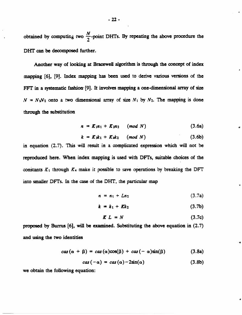


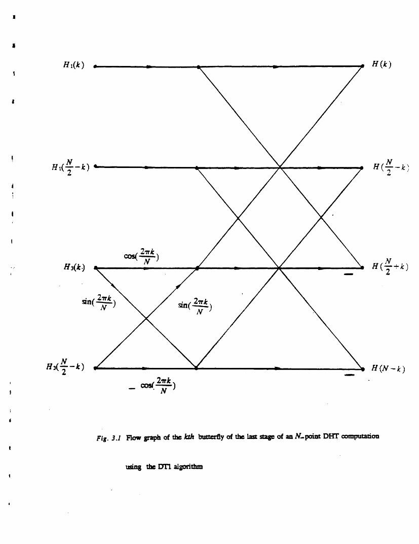


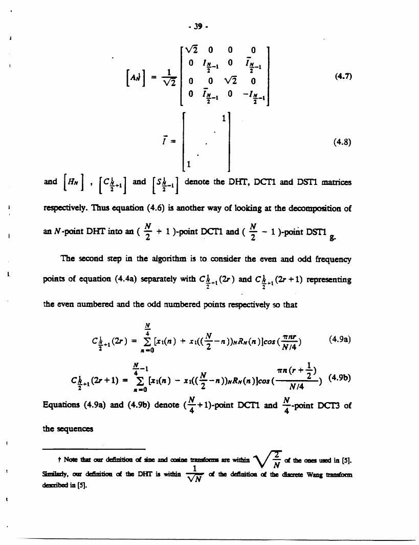


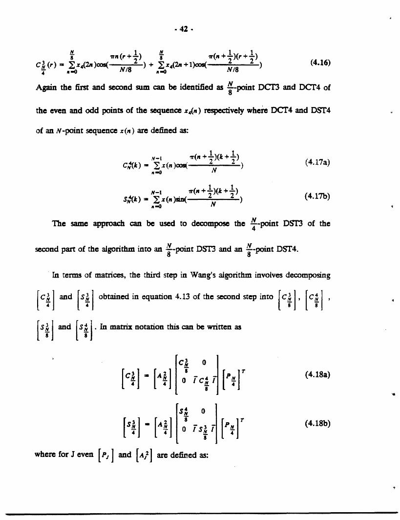
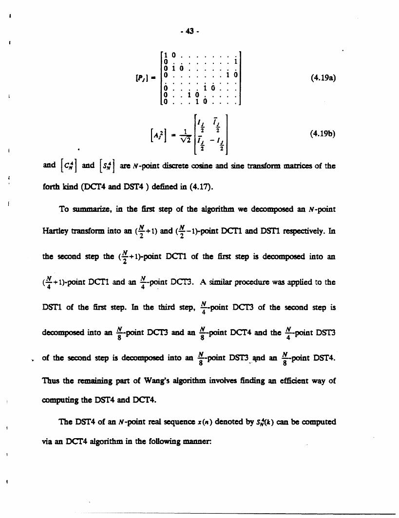
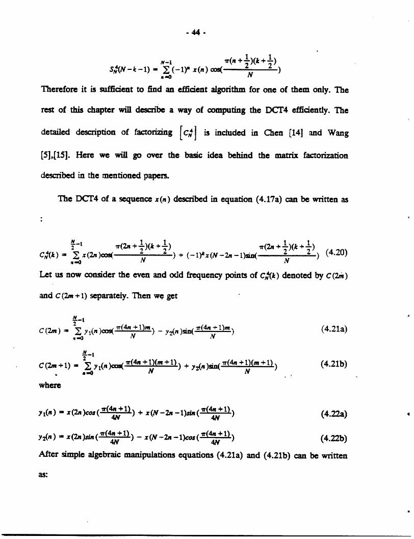


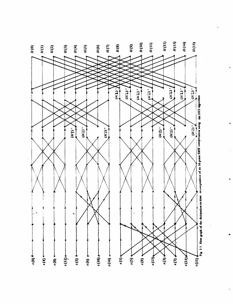

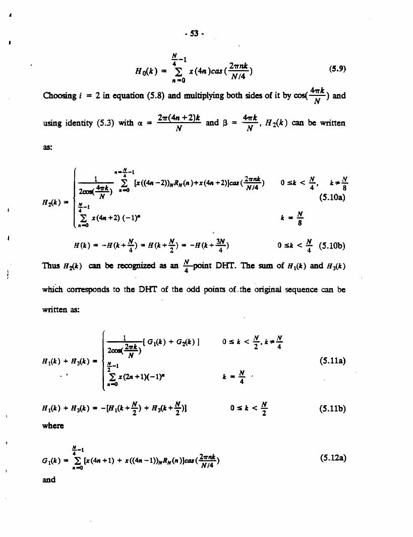


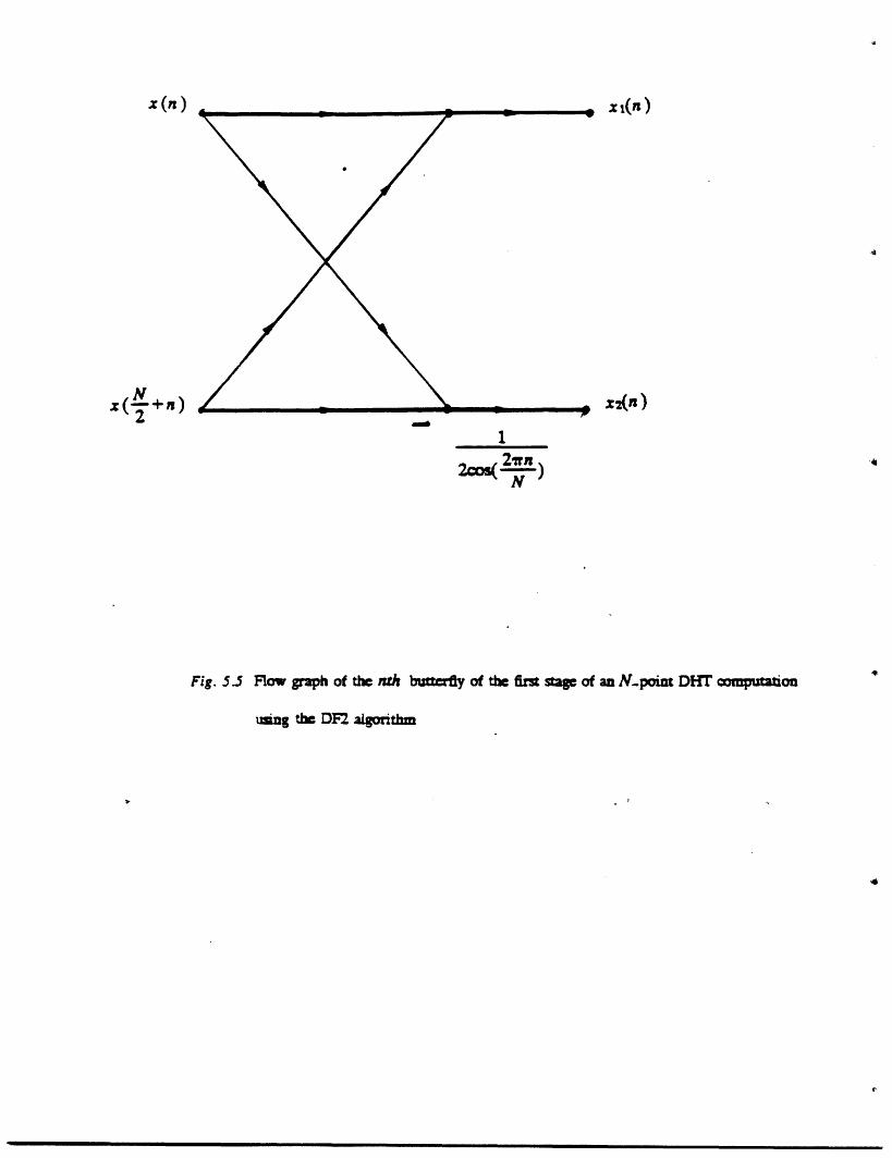
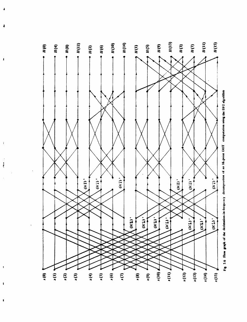


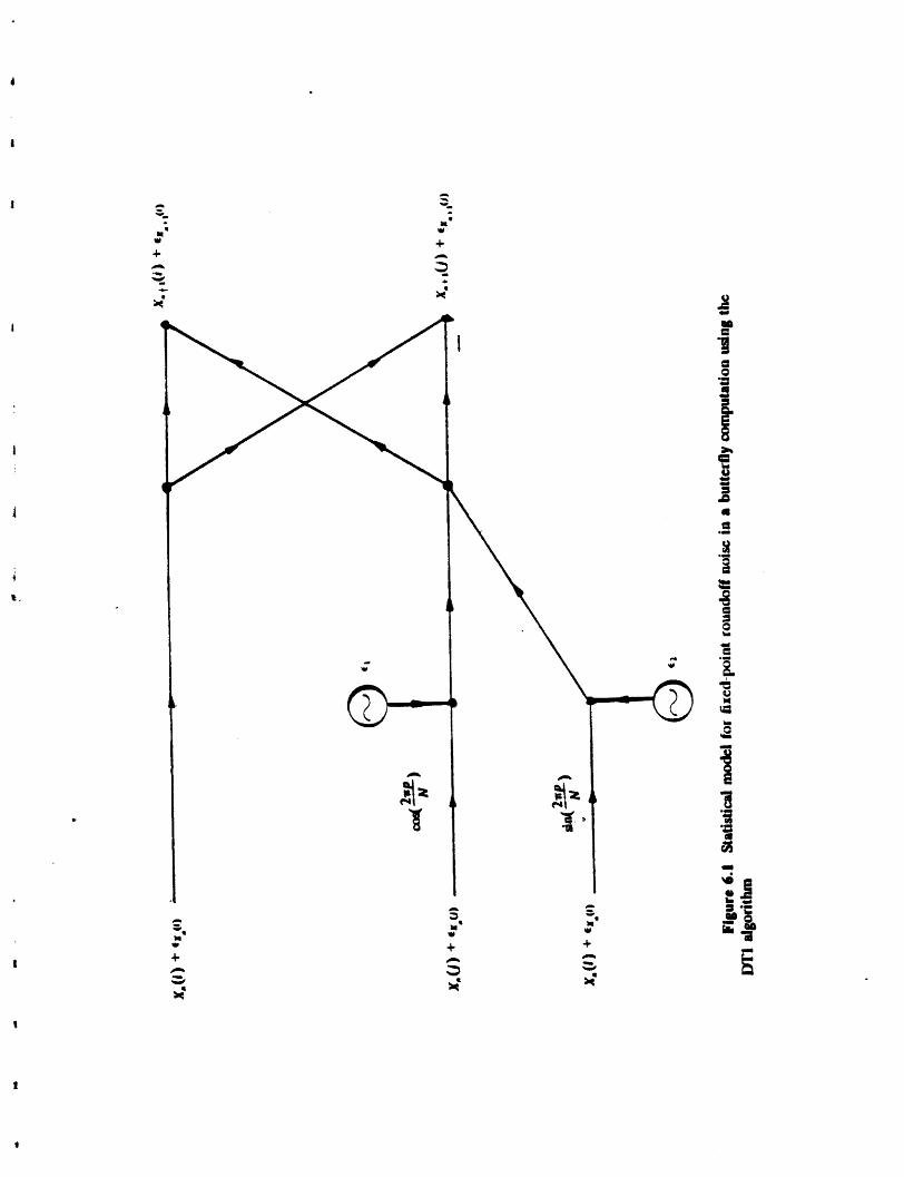


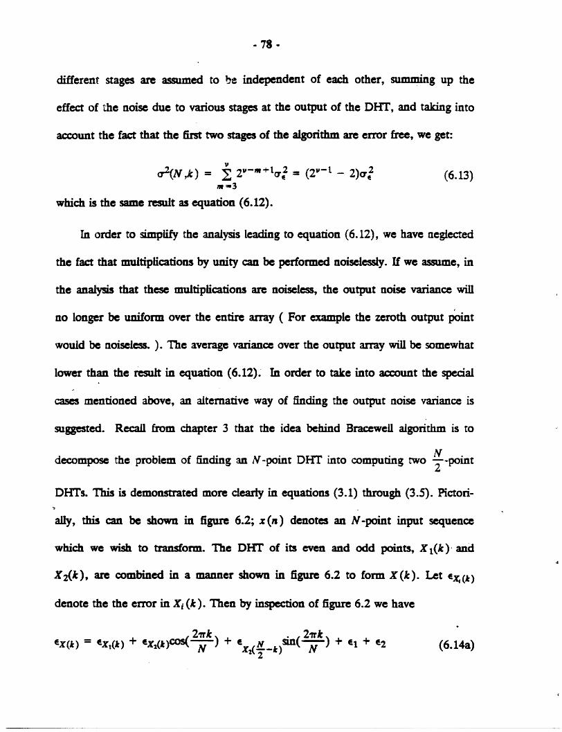

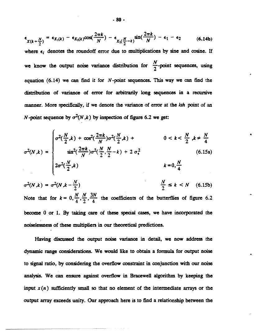


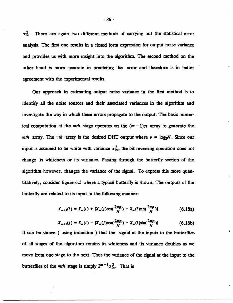
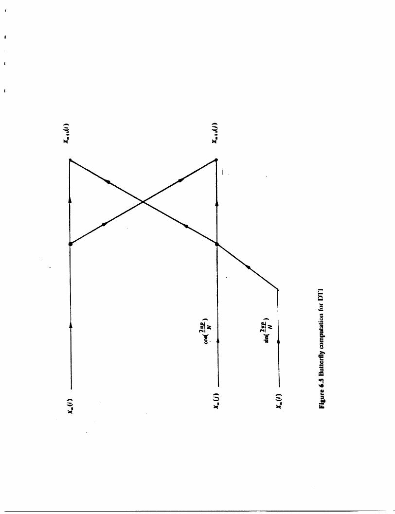


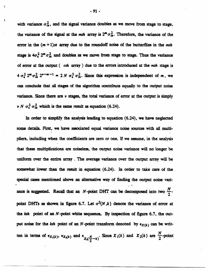
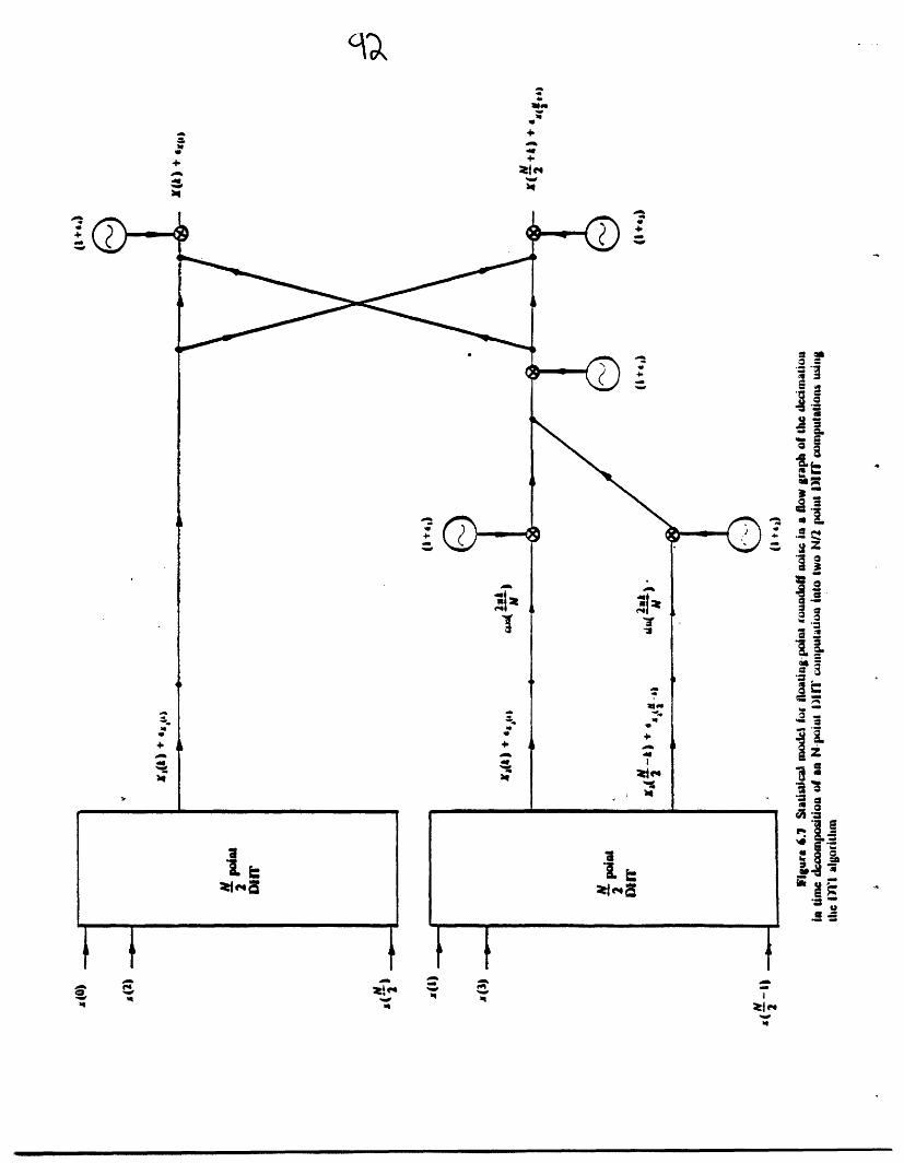


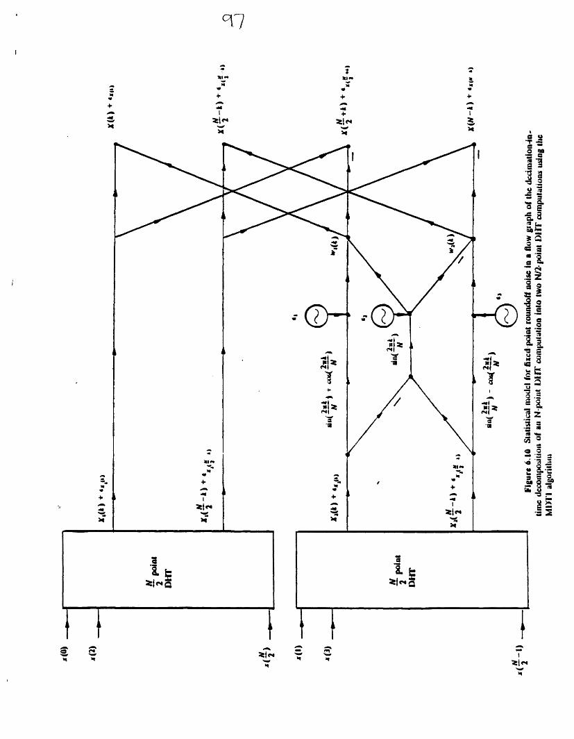

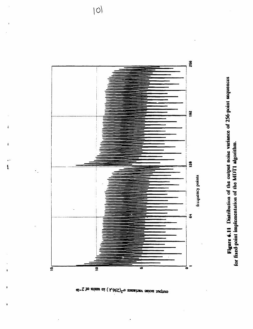

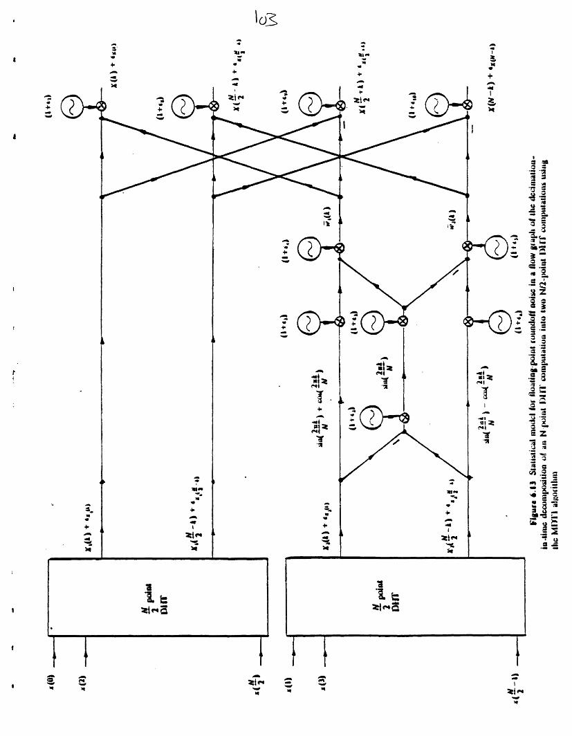

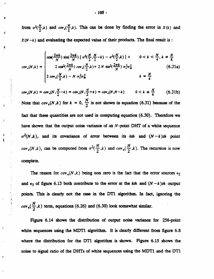
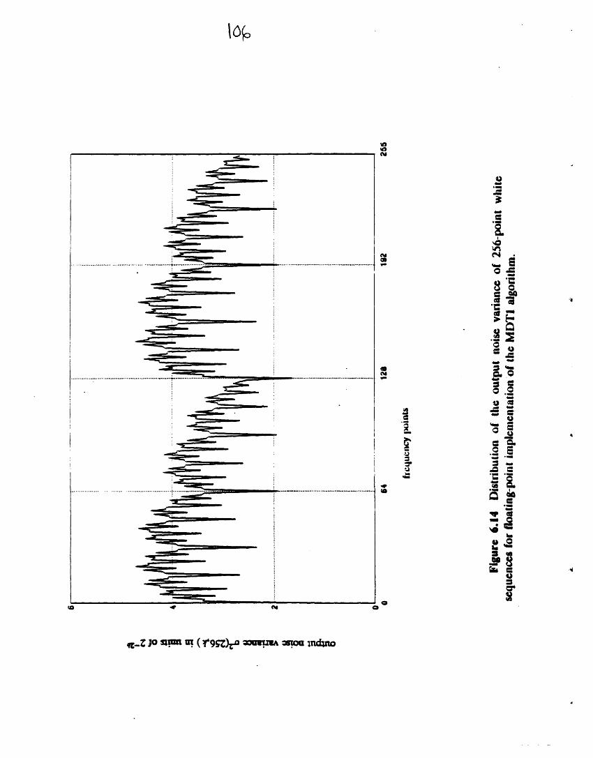


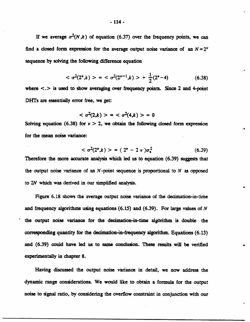
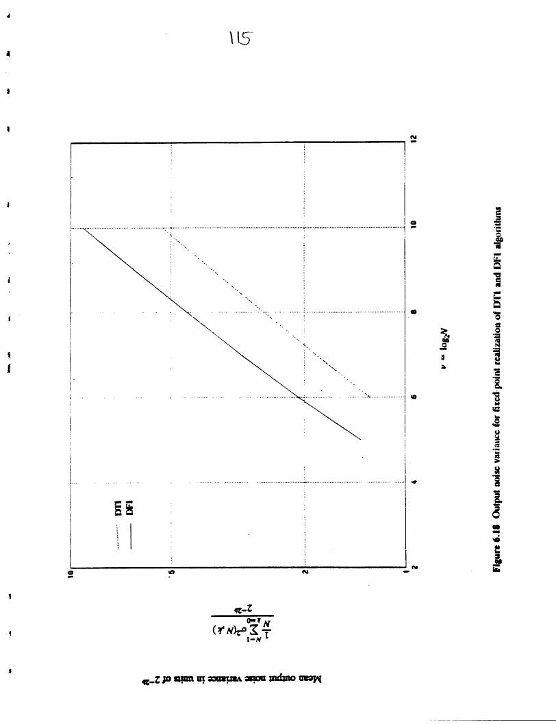


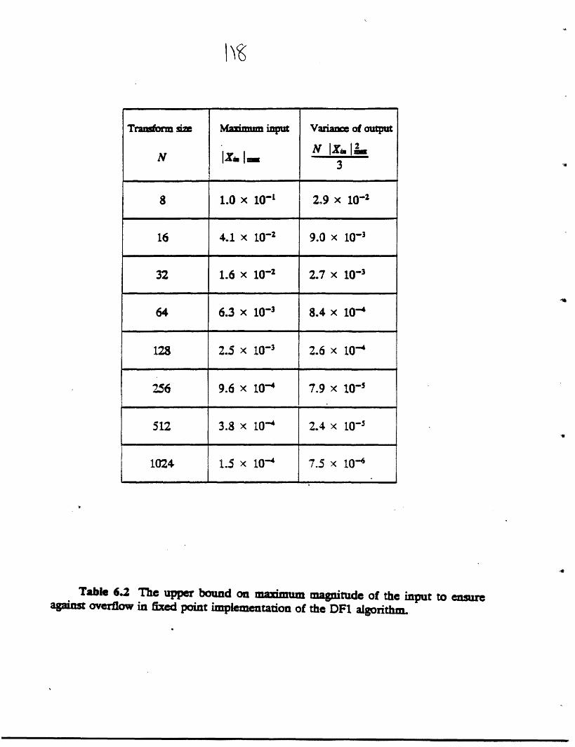
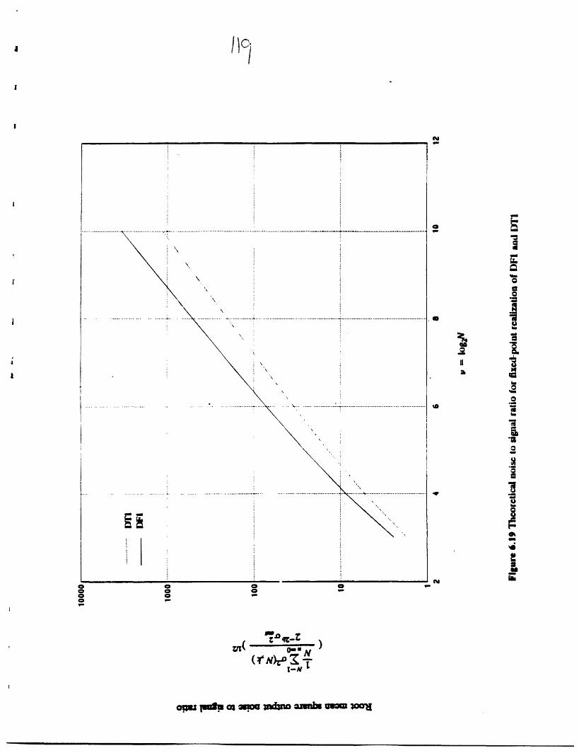
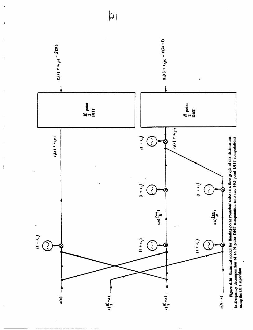


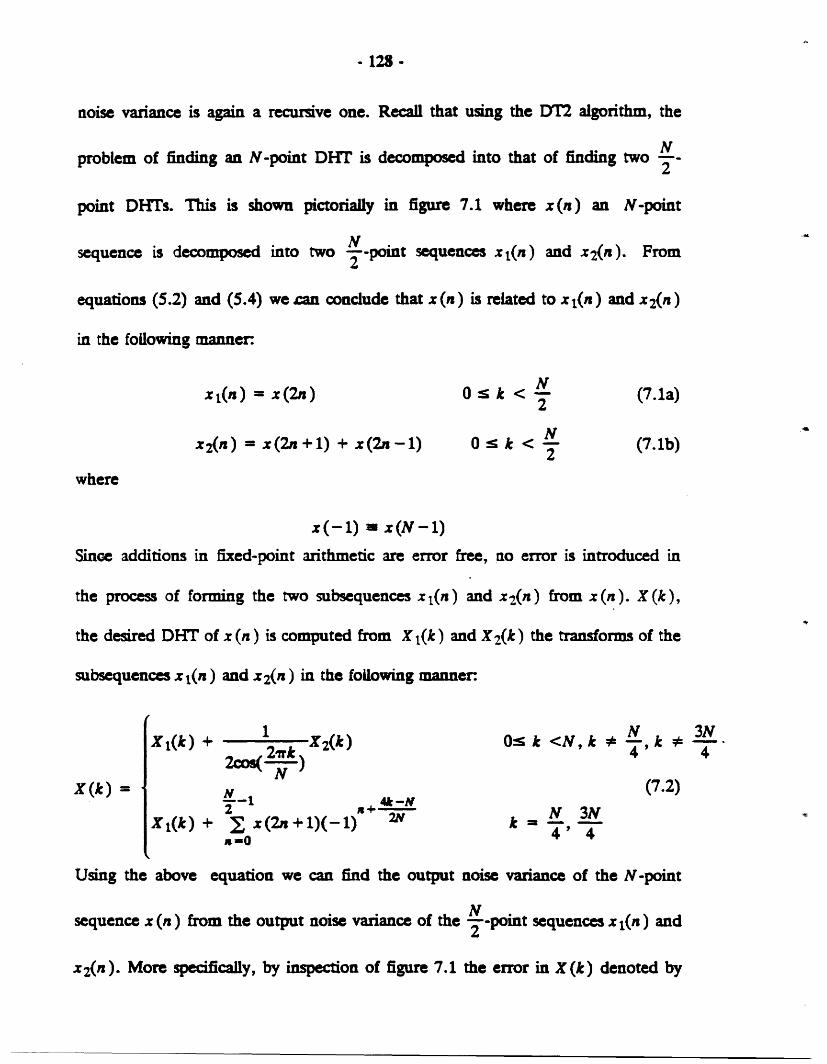
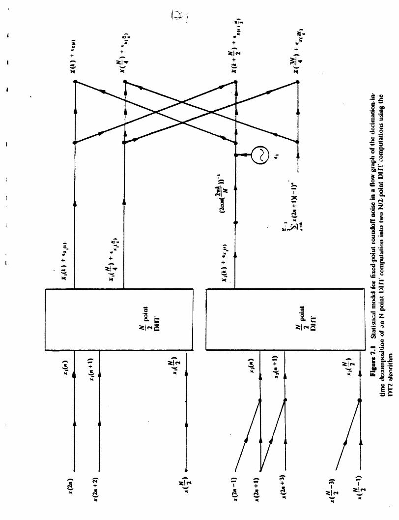


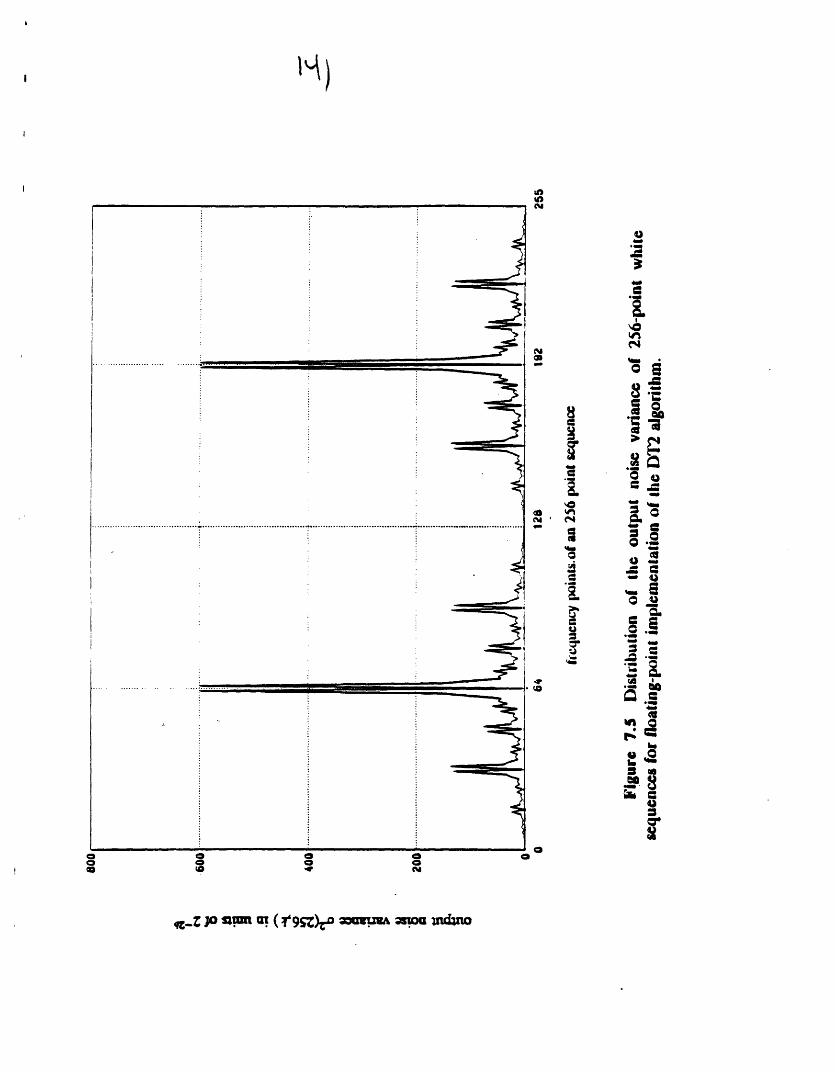
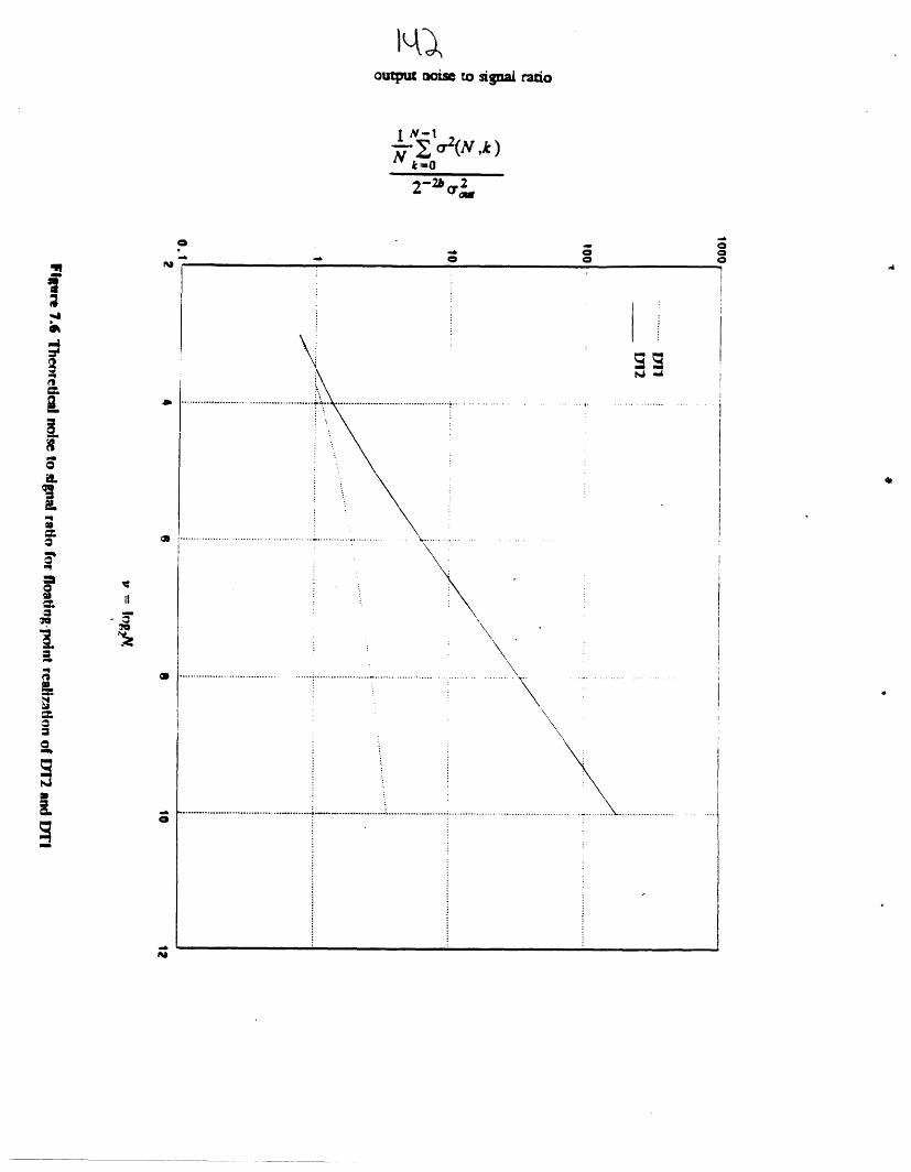
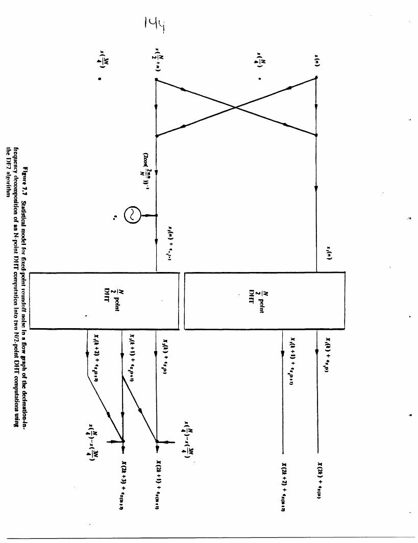
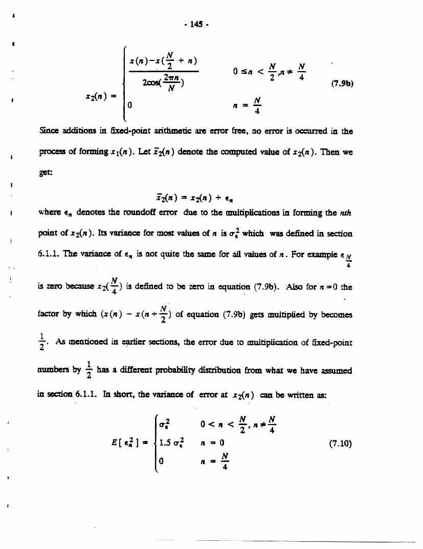

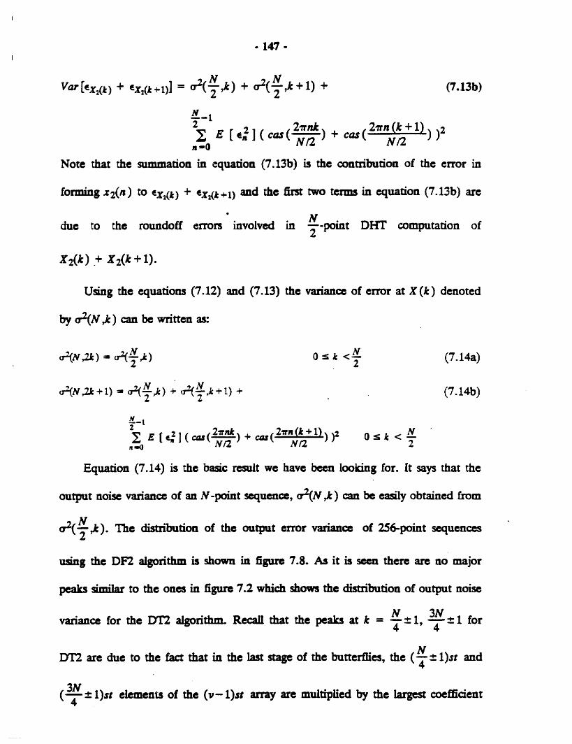


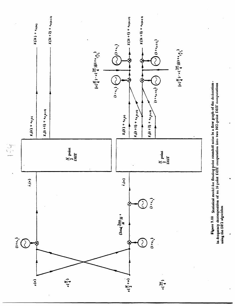


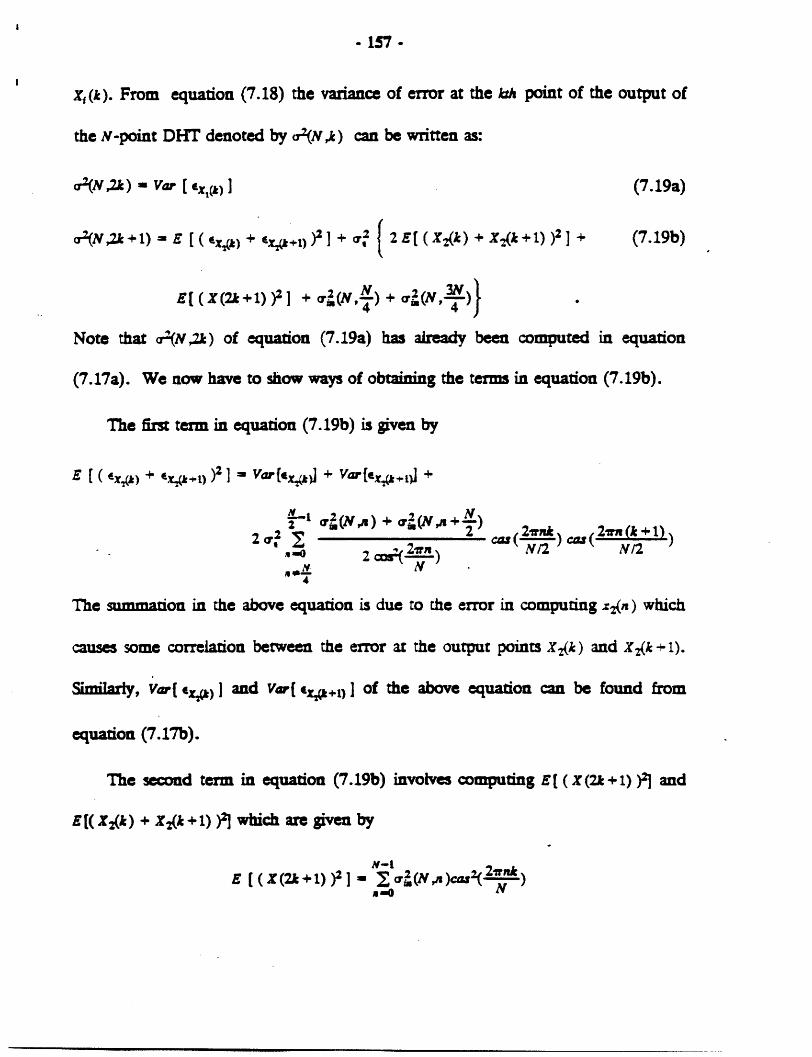


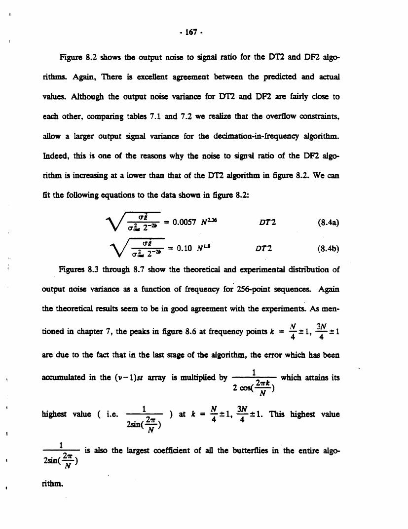
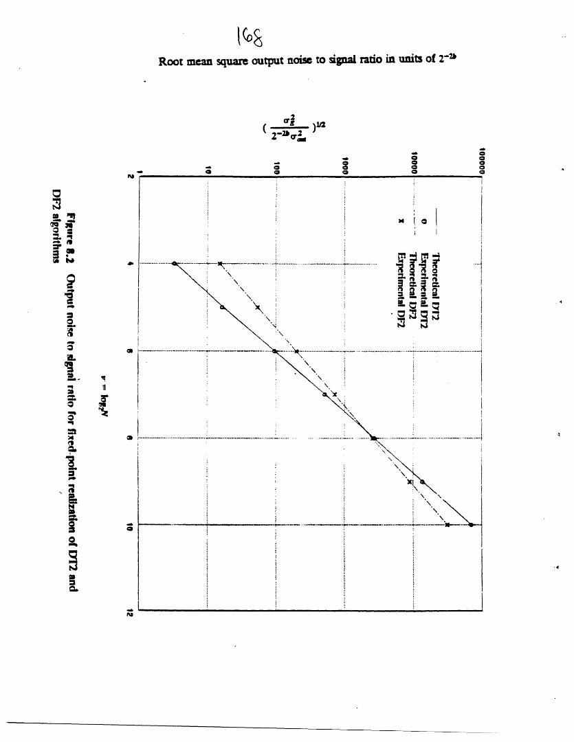
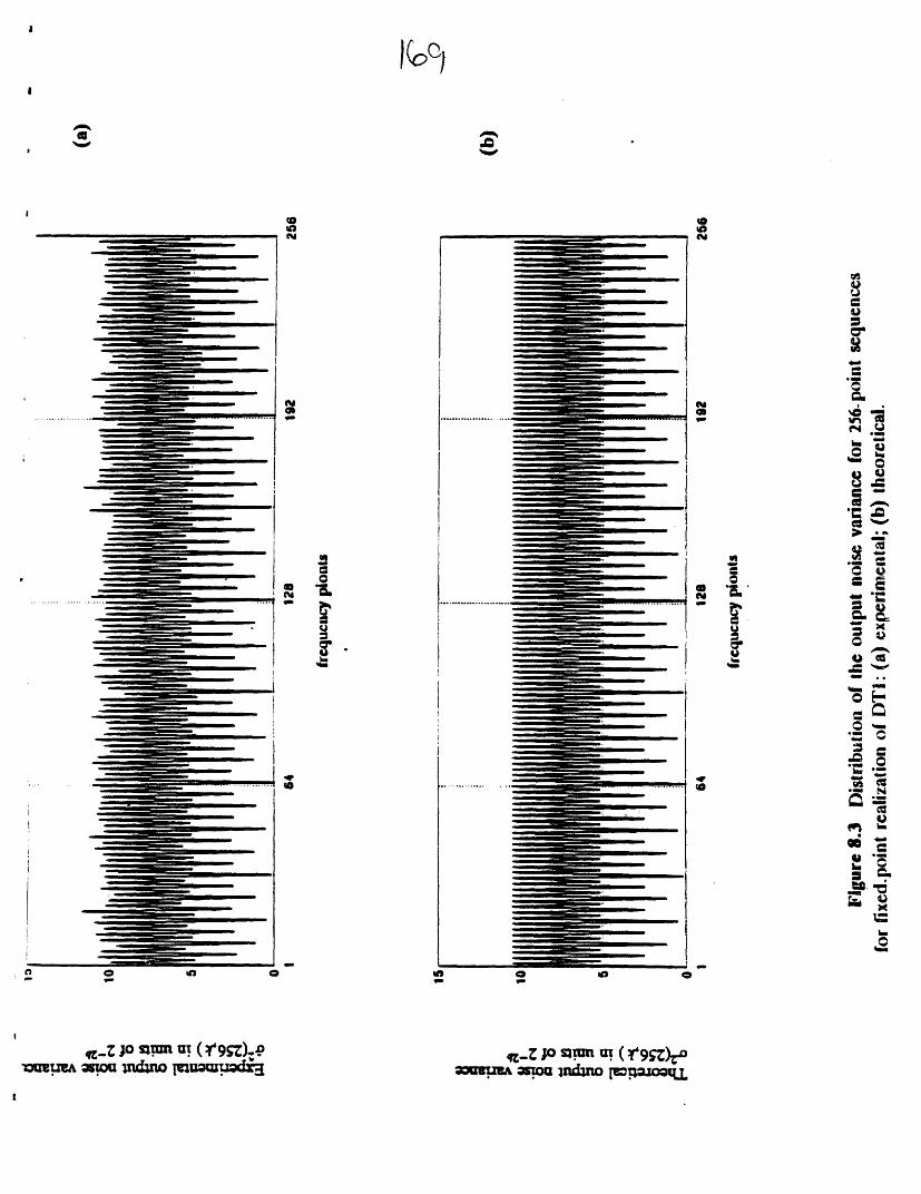


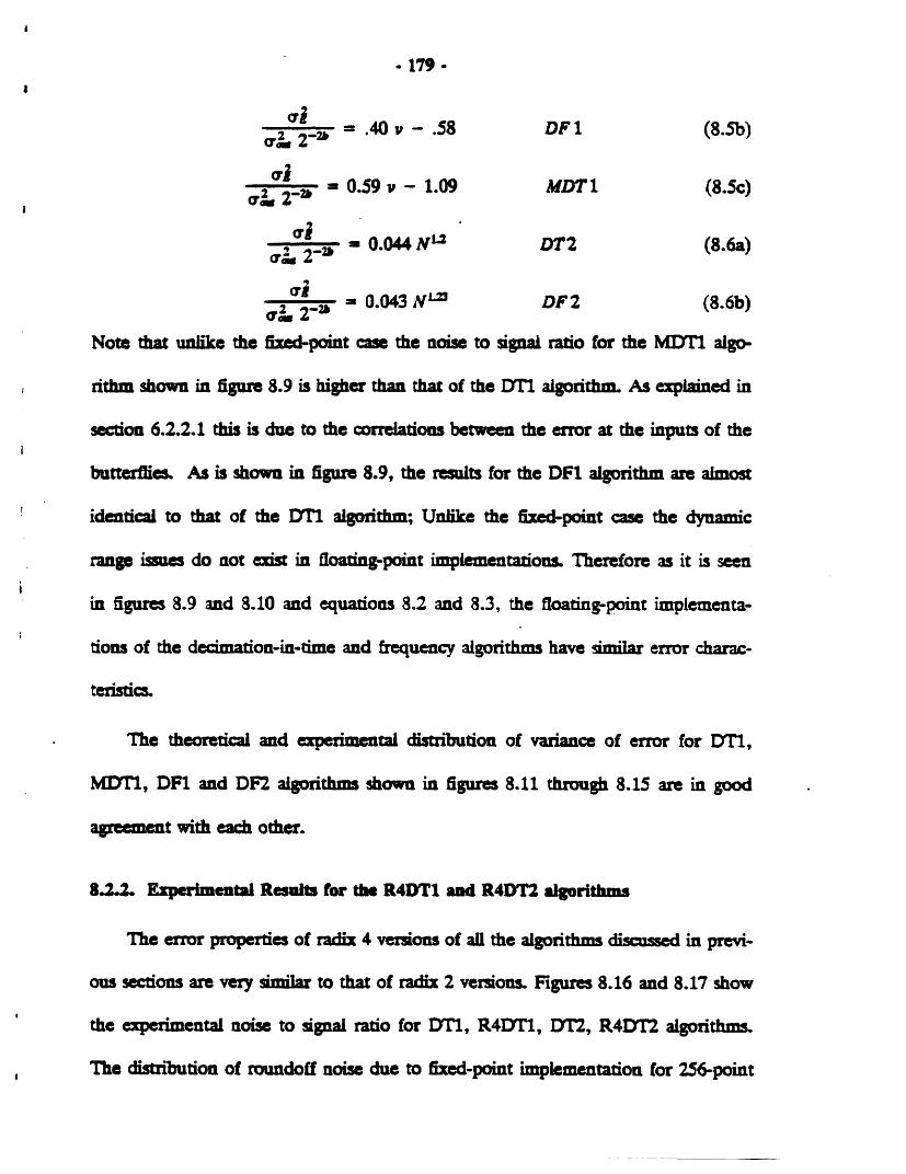
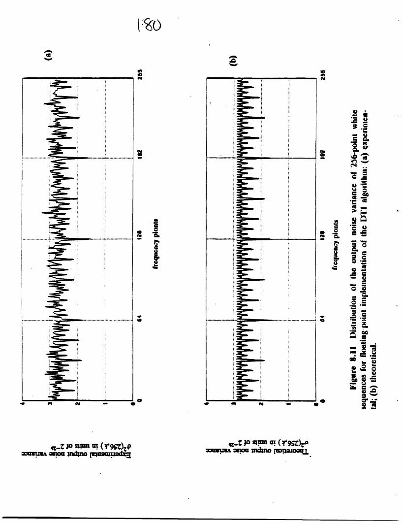
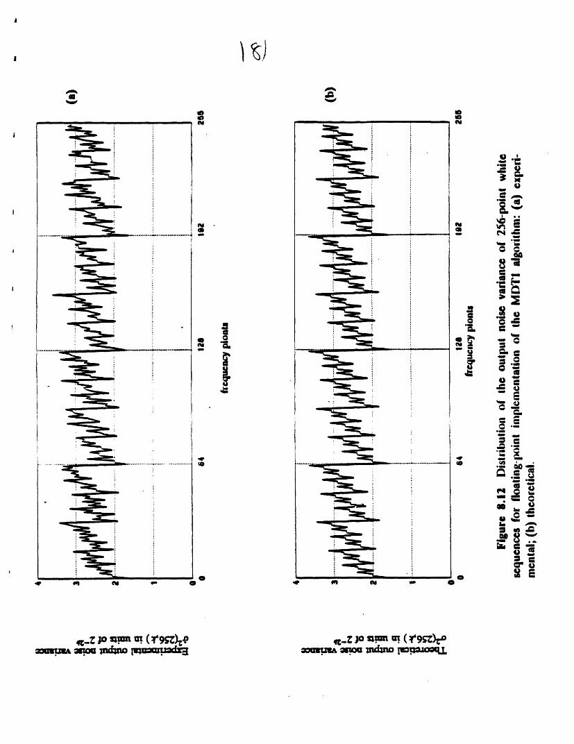


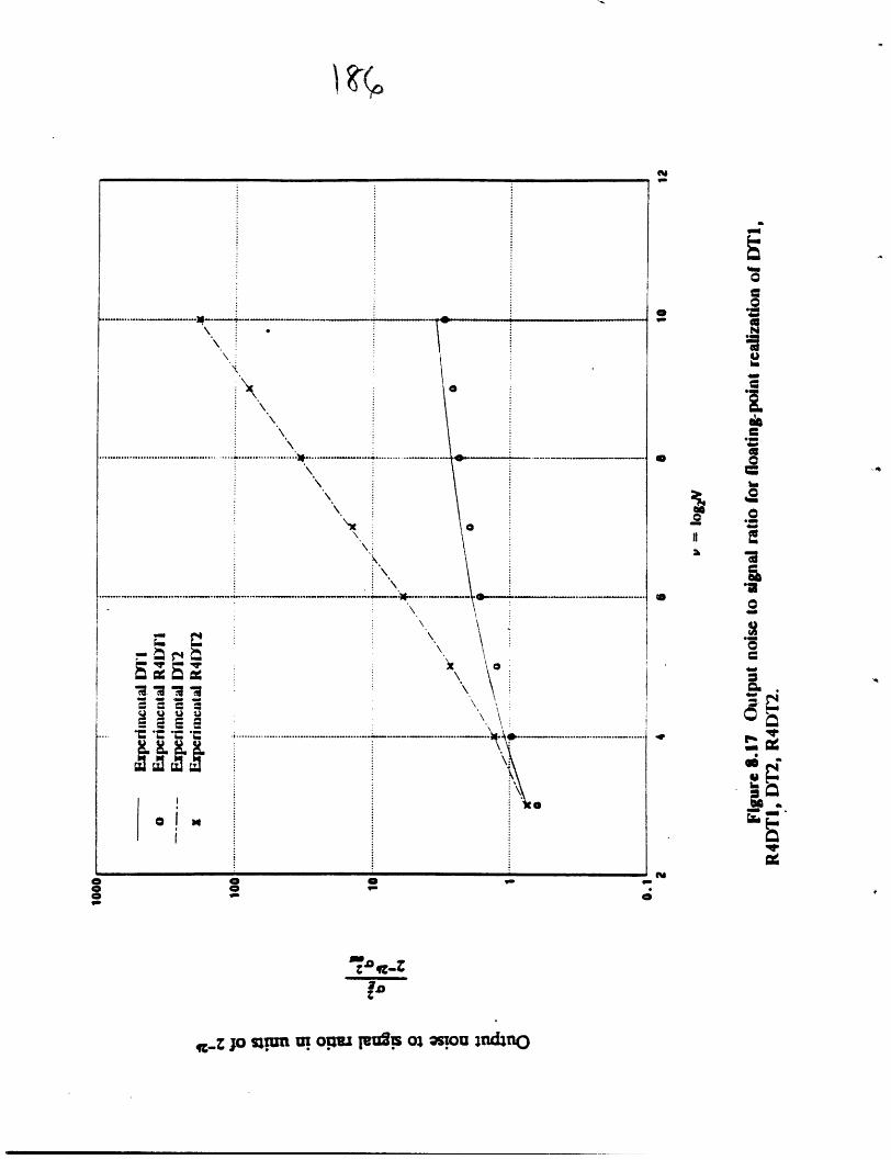


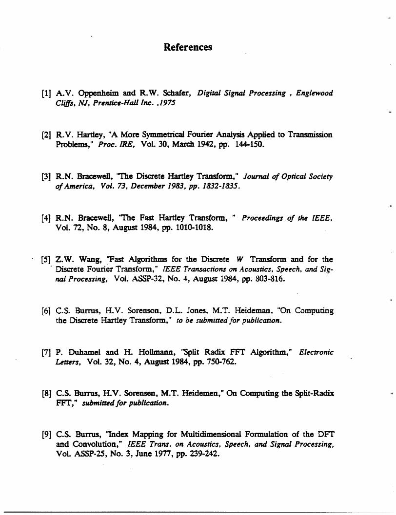


![RLE-TR-413-047432 - [email protected]](https://static.documents.pub/doc/80x56/622c58bb0f6540374178a6e6/rle-tr-413-047432-emailprotected.jpg)


